part 5: random variables 5-1/35 statistics and data analysis professor william greene stern school...
Post on 20-Dec-2015
215 views
TRANSCRIPT
Part 5: Random Variables5-1/35
Statistics and Data Analysis
Professor William Greene
Stern School of Business
IOMS Department
Department of Economics

Part 5: Random Variables5-2/35
Statistics and Data Analysis
Part 5 – Random Variables
Part 5: Random Variables5-3/35
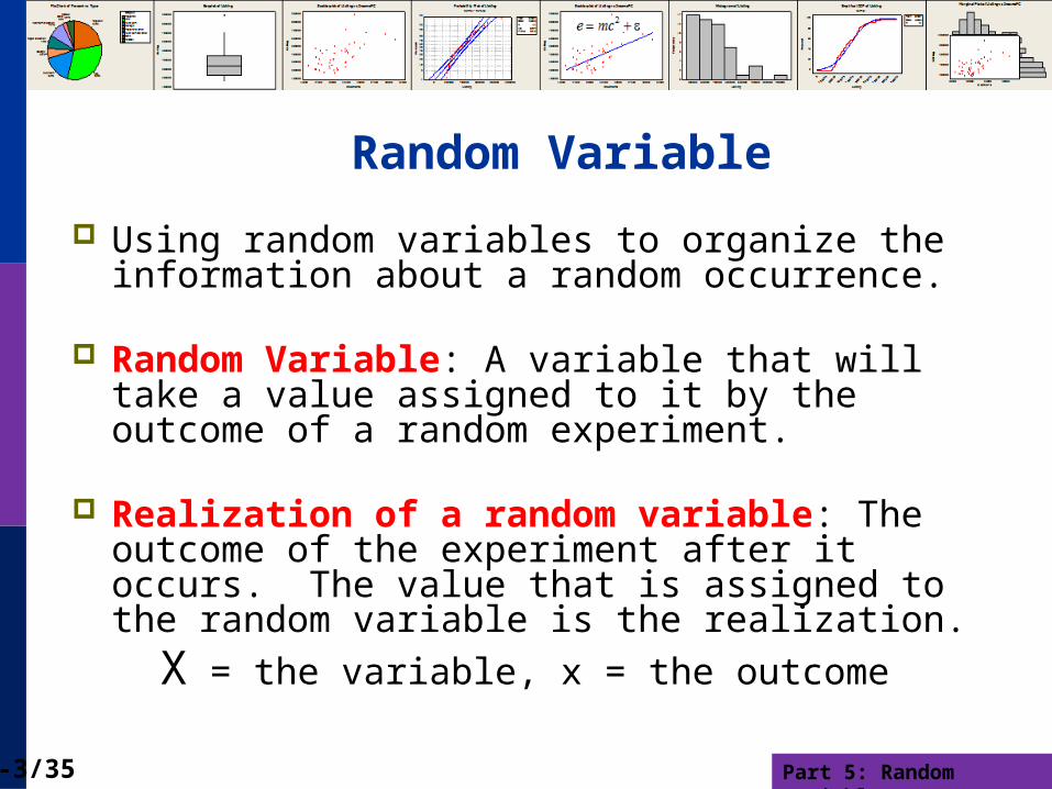
Random Variable
Using random variables to organize the information about a random occurrence.
Random Variable: A variable that will take a value assigned to it by the outcome of a random experiment.
Realization of a random variable: The outcome of the experiment after it occurs. The value that is assigned to the random variable is the realization.
X = the variable, x = the outcome

Part 5: Random Variables5-4/35
Types of Random Variables
Discrete: Takes integer values Binary: Will an individual default (X=1) or not (X=0)? Finite: How many female children in families with 4
children; values = 0,1,2,3,4 Finite: How many eggs in a box of 12 are cracked? Infinite: How many people will catch a certain disease
per year in a given population? Values = 0,1,2,3,… (How can the number be infinite? It is a model.)
Continuous: A measurement. How long will a light bulb last? Values X = 0 to ∞ How do we describe the distribution of biological
measurements? Measures of intellectual performance

Part 5: Random Variables5-5/35
Modeling Fair Isaacs: A Binary Random Variable
Sample of Applicants for a Credit Card (November, 1992)
Experiment = One randomly picked application.
Let X = 0 if Rejected
Let X = 1 if Accepted
X is DISCRETE (Binary). This is called a Bernoulli random variable.
Rejected Approved

Part 5: Random Variables5-6/35
The Random Variable Lenders Are Really Interested In Is Default
Of 10,499 people whose application was accepted, 996 (9.49%) defaulted on their credit account (loan). We let X denote the behavior of a credit card recipient.
X = 0 if no default
X = 1 if default
This is a crucial variable for a lender. They spend endless resources trying to learn more about it.
Part 5: Random Variables5-7/35
Part 5: Random Variables5-8/35
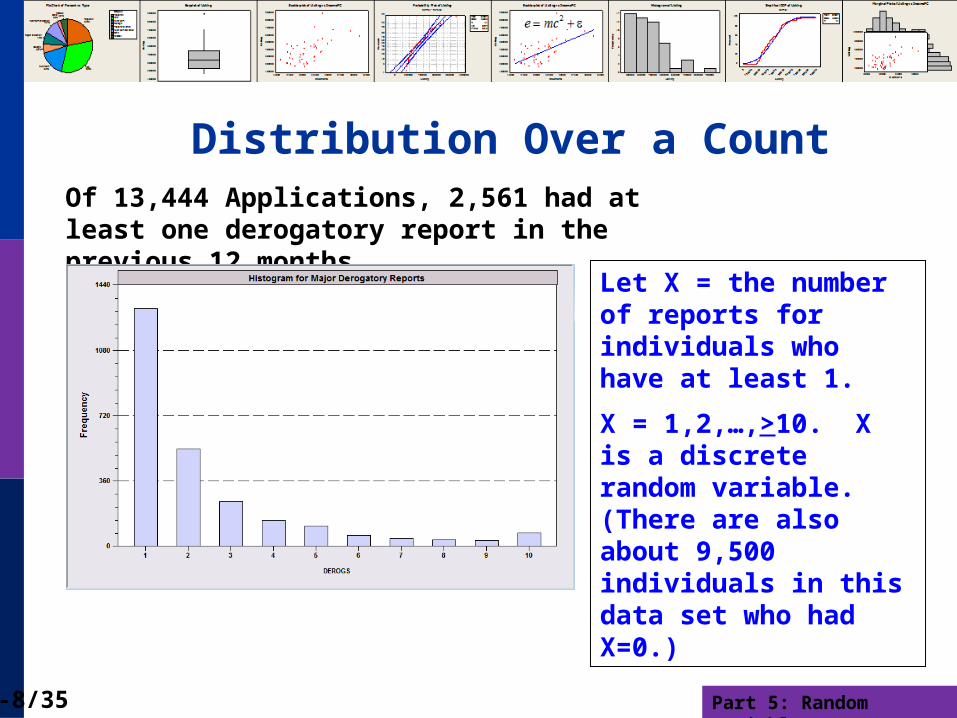
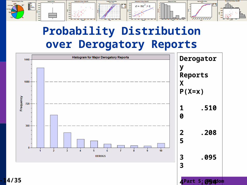
Distribution Over a CountOf 13,444 Applications, 2,561 had at least one derogatory report in the previous 12 months.
Let X = the number of reports for individuals who have at least 1.
X = 1,2,…,>10. X is a discrete random variable. (There are also about 9,500 individuals in this data set who had X=0.)

Part 5: Random Variables5-9/35
Discrete Random Variable?
Response (0 to 10) to the question: How satisfied are you with your health right now?
Experiment = the response of an individual drawn at random.
Let X = their response to the question. X = 0,1,…,10
This is a DISCRETE random variable, but it is not a count.
Do women answer systematically differently from men?

Part 5: Random Variables5-10/35
Continuous Variable – Light Bulb Lifetimes
Probability for a specific value is 0.
Probabilities are defined over intervals, such as
P(1000 < Lifetime < 2500). Needs calculus.
Part 5: Random Variables5-11/35
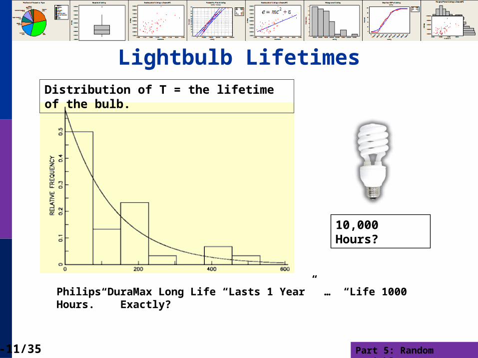
Lightbulb Lifetimes
Philips DuraMax Long Life “Lasts 1 Year” … “Life 1000 Hours.” Exactly?
Distribution of T = the lifetime of the bulb.
10,000 Hours?

Part 5: Random Variables5-12/35
Probability Distribution
Range of the random variable = the set of values it can take Discrete: A set of integers. May be finite or infinite Continuous: A range of values
Probability distribution: Probabilities associated with values in the range.
Part 5: Random Variables5-13/35
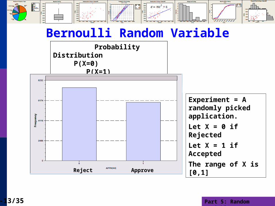
Bernoulli Random Variable
Experiment = A randomly picked application.
Let X = 0 if Rejected
Let X = 1 if Accepted
The range of X is [0,1]
Probability Distribution P(X=0) P(X=1) 0.5556 0.4444
Reject Approve
Part 5: Random Variables5-14/35
Probability Distribution over Derogatory Reports
DerogatoryReportsX P(X=x) 1 .5100 2 .2085 3 .0953 4 .0547 5 .0430 6 .0226 7 .0148 8 .0125 9 .010910 .0277
Part 5: Random Variables5-15/35
Notation
Probability distribution = probabilities assigned to outcomes.
P(X=x) or P(Y=y) is common.
Probability function = PX(x). Sometimes called the density function
Cumulative probability is Prob(X < x) for the specific X.

Part 5: Random Variables5-16/35
Cumulative Probability
Derogatory ReportsX P(X=x) P(X<x) 1 .5100 .5100 2 .2085 .7185 3 .0953 .8138 4 .0547 .8685 5 .0430 .9115 6 .0226 .9341 7 .0148 .9489 8 .0125 .9614 9 .0109 .972310 .0277 1.0000
The item marked 10 is actually 10 or more.
Part 5: Random Variables5-17/35
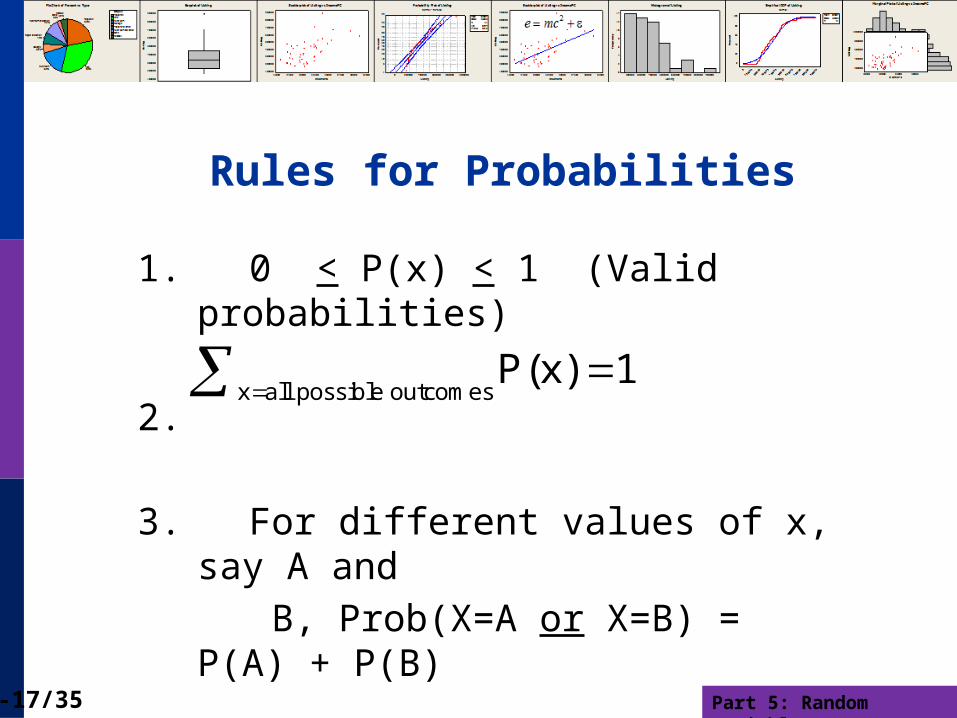
Rules for Probabilities
1. 0 < P(x) < 1 (Valid probabilities)
2.
3. For different values of x, say A and
B, Prob(X=A or X=B) = P(A) + P(B)
x all possible outcomesP(x) 1
Part 5: Random Variables5-18/35
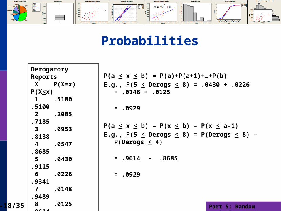
Probabilities
P(a < x < b) = P(a)+P(a+1)+…+P(b)
E.g., P(5 < Derogs < 8) = .0430 + .0226 + .0148 + .0125
= .0929
P(a < x < b) = P(x < b) – P(x < a-1)
E.g., P(5 < Derogs < 8) = P(Derogs < 8) – P(Derogs < 4)
= .9614 - .8685
= .0929
Derogatory Reports X P(X=x) P(X<x) 1 .5100 .5100 2 .2085 .7185 3 .0953 .8138 4 .0547 .8685 5 .0430 .9115 6 .0226 .9341 7 .0148 .9489 8 .0125 .9614 9 .0109 .972310 .0277 1.0000
Part 5: Random Variables5-19/35
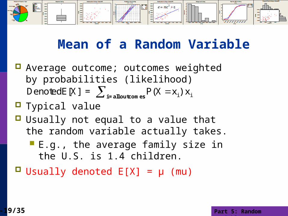
Mean of a Random Variable
Average outcome; outcomes weighted by probabilities (likelihood)
Typical value Usually not equal to a value that the random
variable actually takes. E.g., the average family size in the U.S. is
1.4 children. Usually denoted E[X] = μ (mu)
i iDenotedE[X] = P(X x ) xi = all outcomes
Part 5: Random Variables5-20/35
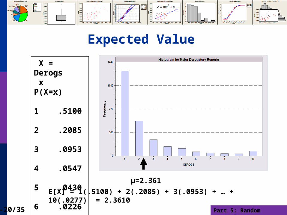
Expected Value
X = Derogs x P(X=x) 1 .5100 2 .2085 3 .0953 4 .0547 5 .0430 6 .0226 7 .0148 8 .0125 9 .010910 .0277
E[X] = 1(.5100) + 2(.2085) + 3(.0953) + … + 10(.0277) = 2.3610
μ=2.361
Part 5: Random Variables5-21/35
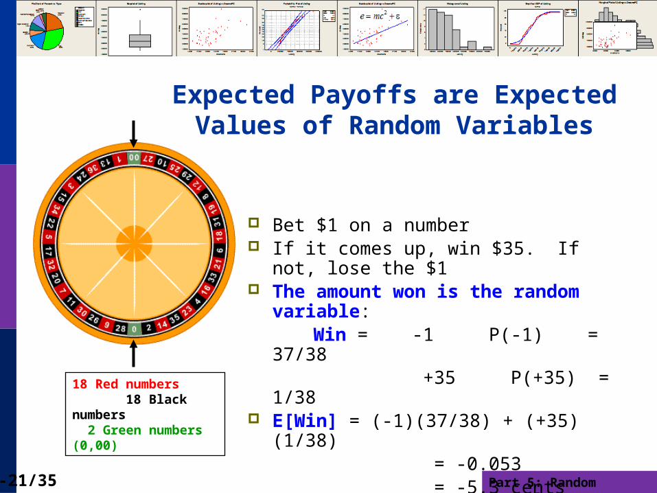
Expected Payoffs are Expected Values of Random Variables
Bet $1 on a number If it comes up, win $35. If not, lose the $1 The amount won is the random variable: Win = -1 P(-1) = 37/38 +35 P(+35) = 1/38 E[Win] = (-1)(37/38) + (+35)(1/38) = -0.053 = -5.3 cents (familiar).18 Red numbers
18 Black numbers 2 Green numbers (0,00)
Part 5: Random Variables5-22/35
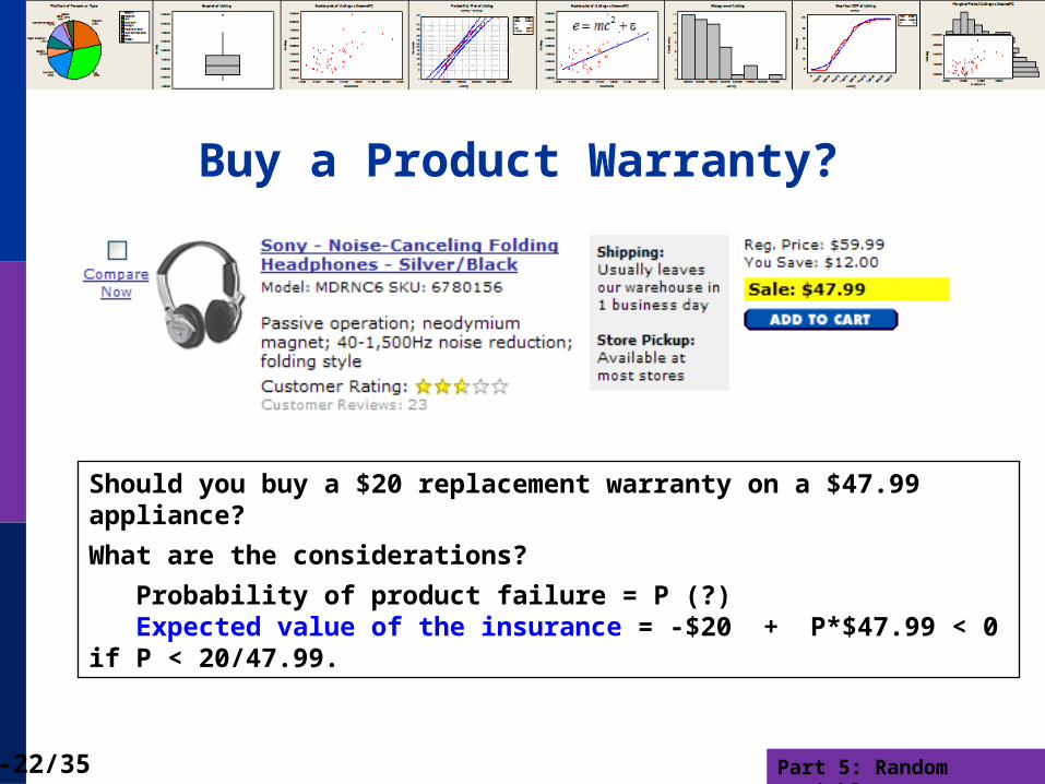
Buy a Product Warranty?
Should you buy a $20 replacement warranty on a $47.99 appliance?
What are the considerations?
Probability of product failure = P (?) Expected value of the insurance = -$20 + P*$47.99 < 0 if P < 20/47.99.

Part 5: Random Variables5-23/35
Median of a Random VariableThe median of X is the value x such that Prob(X < x) = .5.For a continuous variable, we will find this using calculus.For a discrete value, Prob(X < M+1) > .5 and Prob(X < M-1) < .5
X Prob(X=x) Prob(X < x) 0 .0164 .0164 1 .0093 .0257 2 .0235 .0492 3 .0429 .0921 4 .0509 .1430 5 .1549 .2979 6 .0926 .3905 7 .1548 .5453 8 .2259 .7712 9 .1120 .883210 .1168 1.0000
Health Satisfaction Sample Proportions.
Mean (6.8)
Median (7)

Part 5: Random Variables5-24/35
Measuring the “Spread” of the Random Outcomes
DerogatoryReportsX P(X=x) 1 .5100 2 .2085 3 .0953 4 .0547 5 .0430 6 .0226 7 .0148 8 .0125 9 .010910 .0277
μ=2.361
The range is 1 to 10, but values outside 1 to 5 are rather unlikely.
Part 5: Random Variables5-25/35
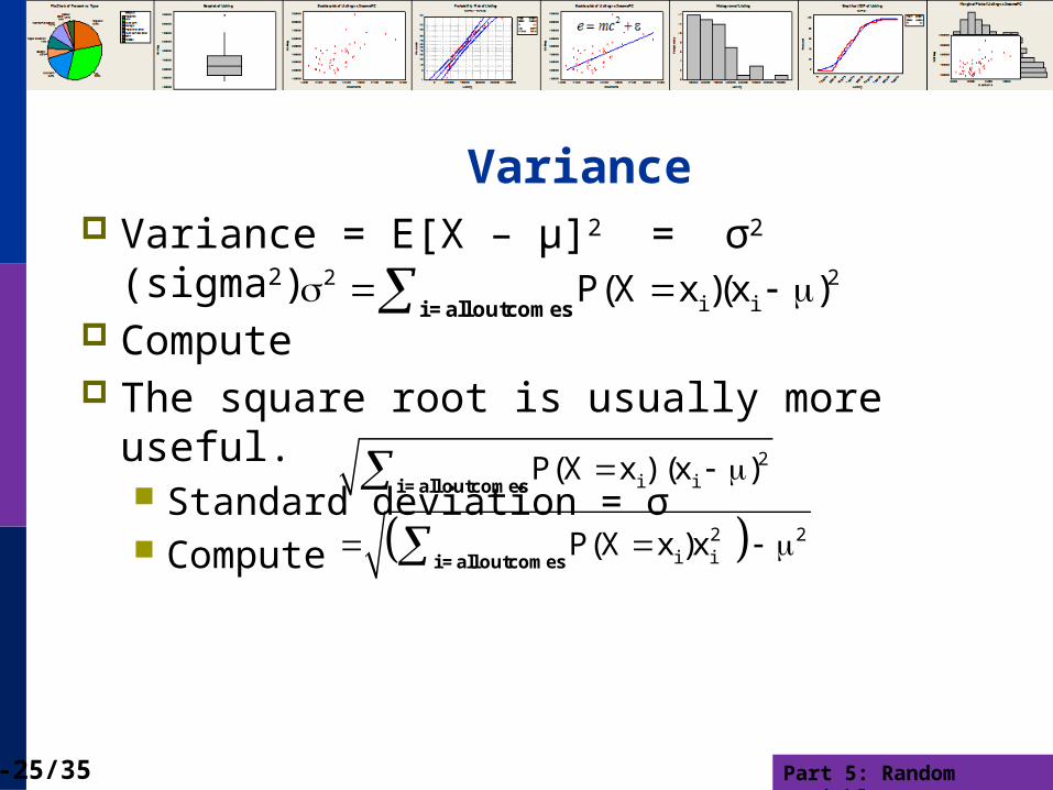
Variance Variance = E[X – μ]2 = σ2 (sigma2) Compute The square root is usually more useful.
Standard deviation = σ Compute
2 2i iP(X x )(x )
i = all outcomes
2i i
2 2i i
P(X x ) (x )
P(X x )x
i = all outcomes
i = all outcomes
Part 5: Random Variables5-26/35
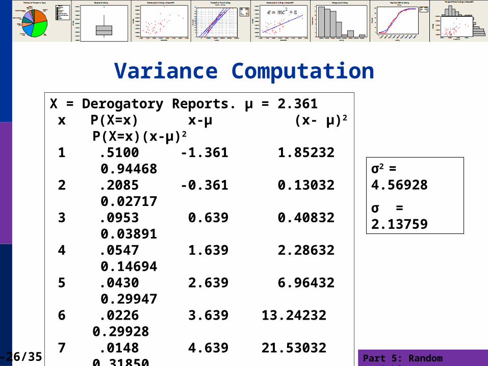
Variance ComputationX = Derogatory Reports. μ = 2.361 x P(X=x) x-μ (x- μ)2 P(X=x)(x-μ)2 1 .5100 -1.361 1.85232 0.94468 2 .2085 -0.361 0.13032 0.02717 3 .0953 0.639 0.40832 0.03891 4 .0547 1.639 2.28632 0.14694 5 .0430 2.639 6.96432 0.29947 6 .0226 3.639 13.24232 0.29928 7 .0148 4.639 21.53032 0.31850 8 .0125 5.639 31.79832 0.39748 9 .0109 6.639 44.07632 0.4804310 .0277 7.639 58.35432 1.61641 SUM 4.56928
σ2 = 4.56928
σ = 2.13759

Part 5: Random Variables5-27/35
Common Results for Random Variables
Concentration of Probability For almost any random variable, 2/3 of the probability
lies within μ ± 1σ For almost any random variable, 95% of the
probability lies within μ ± 2σ For almost any random variable, more than 99.5% of
the probability lies within μ ± 3σ What it means: For any random outcome,
An (observed) outcome more than one σ away from μ is somewhat unusual.
One that is more than 2σ away is very unusual. One that is more than 3σ away from the mean is so
unusual that it might be an outlier (a freak outcome).
Part 5: Random Variables5-28/35
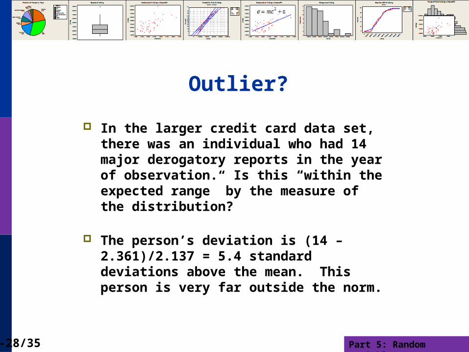
Outlier?
In the larger credit card data set, there was an individual who had 14 major derogatory reports in the year of observation. Is this “within the expected range” by the measure of the distribution?
The person’s deviation is (14 – 2.361)/2.137 = 5.4 standard deviations above the mean. This person is very far outside the norm.

Part 5: Random Variables5-29/35
Reliable Rules of Thumb
Almost always, 66% of the observations in a sample will lie in the range
[mean+1 s.d. and mean – 1 s.d.] Almost always, 95% of the observations in a sample will
lie in the range
[mean+2 s.d. and mean – 2 s.d.] Almost always, 99.5% of the observations in a sample
will lie in the range
[mean+3 s.d. and mean – 3 s.d.]
Recall from day 2 of class
Part 5: Random Variables5-30/35
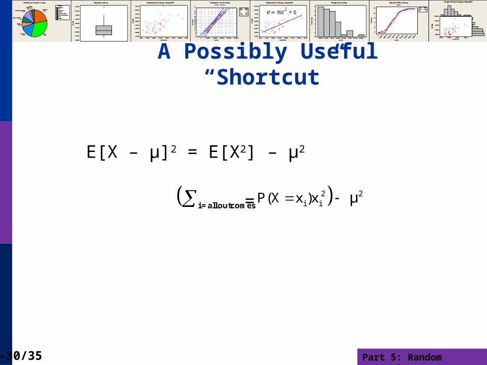
A Possibly Useful “Shortcut”
E[X – μ]2 = E[X2] – μ2
= 2 2i iP(X x )x μ
i = all outcomes

Part 5: Random Variables5-31/35
ApplicationPartyPlanners plans parties each day, and must order supplies for the events.
The number of requests for party plans varies day by day according to
P(X=0) = .4 P(X=1) = .3 P(X=2) = .25 P(X=3) = .05
H
2 2 2 2
ow many parties should they expect on a given day?
E[X] = .4(0) + .3(1) + .25(2) + .05(3) = .95, or about 1.
What are the variance and standard deviation?
Var[X] = .4(0 )+ .3(1 ) + .25(2 ) + .05(3 ) -.952 = .8475. 0.8475 = 0.9206
If they plan for 1 party per day, it is rather likely that they will run out of materials
since 2 is only 1.1 standard deviations above the mean.

Part 5: Random Variables5-32/35
Important Algebra
Linear Translation: For the random variable X with mean E[X] = μ,
if Y = a+bX, then E[Y] = a + bμ Scaling: For the random variable X with
standard deviation σX,
if Y = a+bX, then σY = |b| σX
It is not necessary to transform the original data.

Part 5: Random Variables5-33/35
Example: Repair Costs The number of repair orders per day at a body shop is distributed by:
Repairs 0 1 2 3 4Probability .1 .2 .35 .2 .15
Opening the shop costs $500 for any repairs. Two people each cost $100/repair to do the work.
What are the mean and standard deviation of the number of repair orders?μ = 0(.1) + 1(.2) + 2(.35) + 3(.2) + 4(.15) = 2.10σ2 = 02(.1) + 12(.2) + 22(.35) + 32(.2) + 42(.15) – 2.12 = 1.39σ = 1.179
What are the mean and standard deviation of the cost per day to run the shop?Cost = $500 + $100*(2)*(Number of Repairs)Mean = $500 + $200*(2.1) = $920/dayStandard deviation = $200(1.179) = $235.80/day
Part 5: Random Variables5-34/35
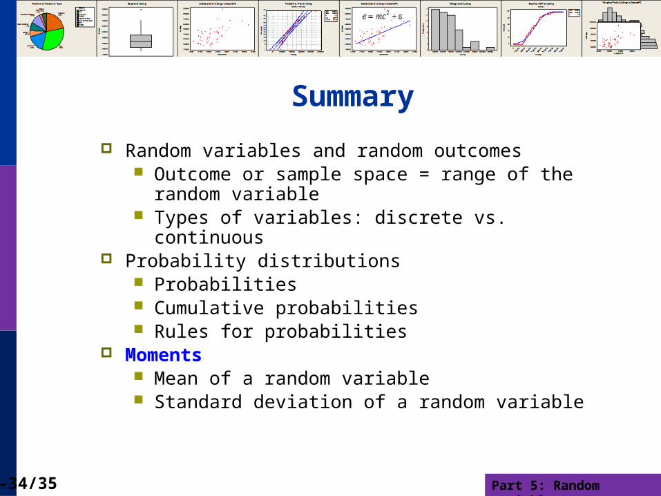
Summary
Random variables and random outcomes Outcome or sample space = range of the random
variable Types of variables: discrete vs. continuous
Probability distributions Probabilities Cumulative probabilities Rules for probabilities
Moments Mean of a random variable Standard deviation of a random variable
Part 5: Random Variables5-35/35
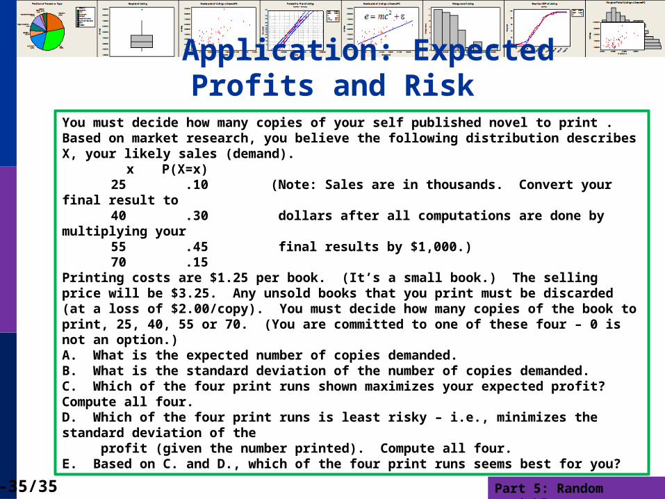
Application: Expected Profits and RiskYou must decide how many copies of your self published novel to print . Based on market research, you believe the following distribution describes X, your likely sales (demand).
x P(X=x) 25 .10 (Note: Sales are in thousands. Convert your final result to 40 .30 dollars after all computations are done by multiplying your 55 .45 final results by $1,000.) 70 .15
Printing costs are $1.25 per book. (It’s a small book.) The selling price will be $3.25. Any unsold books that you print must be discarded (at a loss of $2.00/copy). You must decide how many copies of the book to print, 25, 40, 55 or 70. (You are committed to one of these four – 0 is not an option.)A. What is the expected number of copies demanded.B. What is the standard deviation of the number of copies demanded.C. Which of the four print runs shown maximizes your expected profit? Compute all four.D. Which of the four print runs is least risky – i.e., minimizes the standard deviation of the profit (given the number printed). Compute all four.E. Based on C. and D., which of the four print runs seems best for you?

Part 5: Random Variables5-36/35
all values of x
X = Sales (Demand)
x P(X=x)
25,000 .10
40,000 .30
55,000 .45
70,000 .15
A. Expected Value = x P(X=x)
= .1(25,000) + .3(40,000)
+ .45(55,000) + .15(70,000)
= 49,750
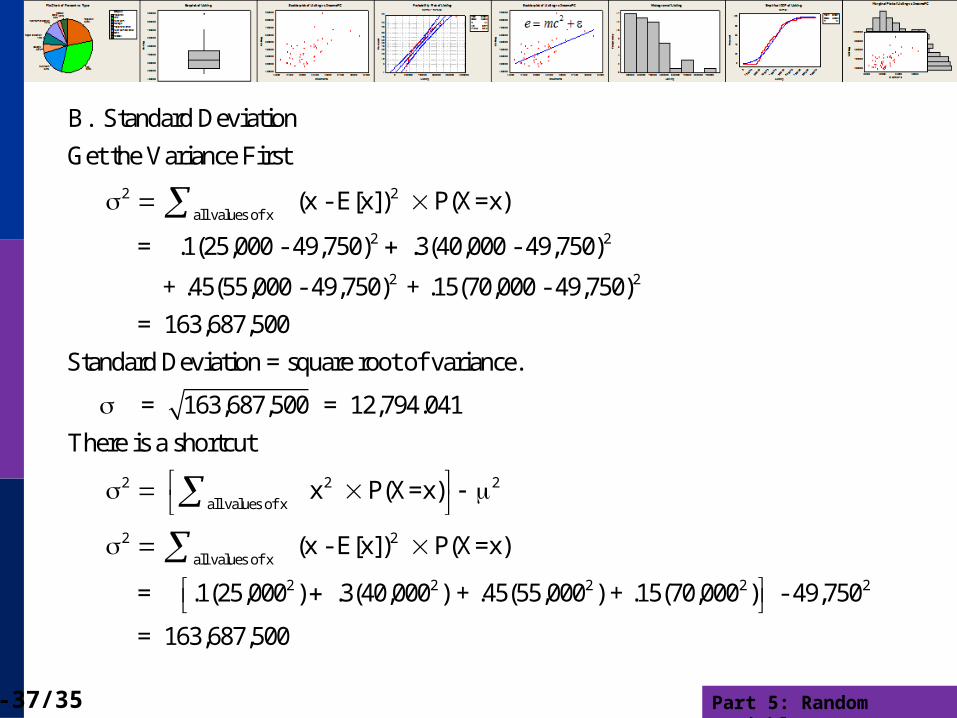
Part 5: Random Variables5-37/35
2 2
all values of x
2 2
2
B. Standard Deviation
Get the Variance First
(x - E[x]) P(X=x)
= .1(25,000 - 49,750) .3(40,000 - 49,750)
+ .45(55,000 - 49,750) + .15(70,000
2
2 2 2
all values of x
2
all va
- 49,750)
= 163,687,500
Standard Deviation = square root of variance.
= 163,687,500 = 12,794.041
There is a shortcut
x P(X=x)
2
lues of x
2 2 2 2 2
(x - E[x]) P(X=x)
= .1(25,000 ) .3(40,000 ) + .45(55,000 ) + .15(70,000 ) - 49,750
= 163,687,500

Part 5: Random Variables5-38/35
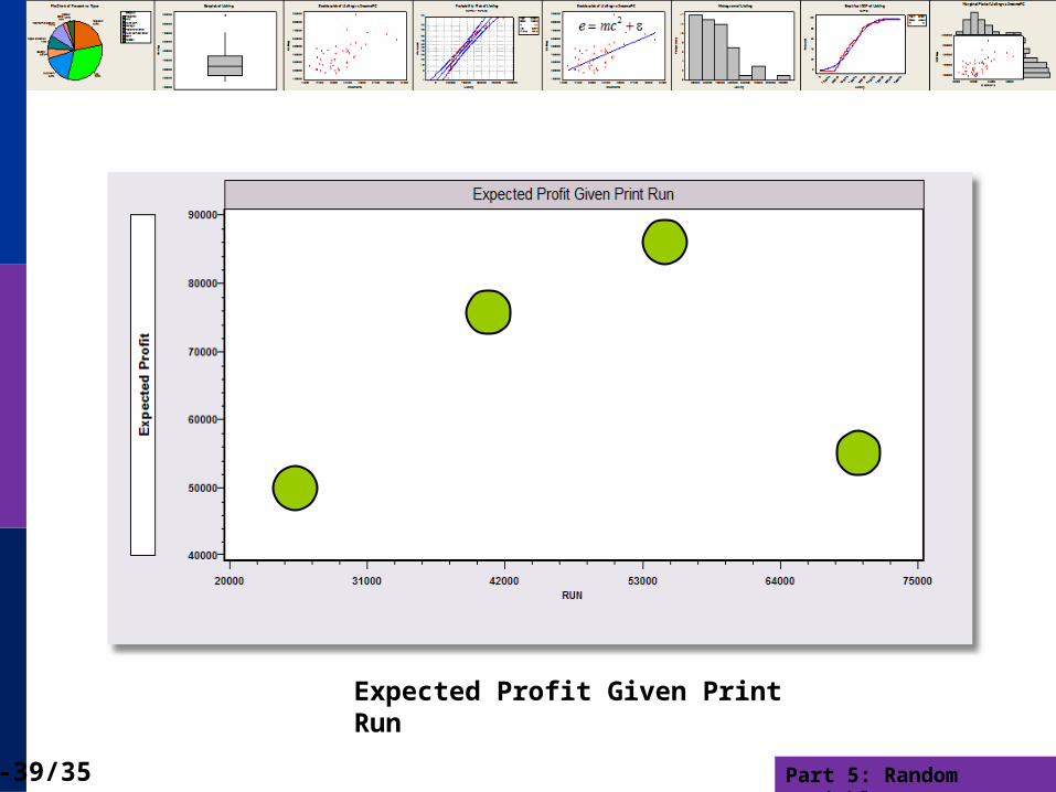
x P(X=x) Revenue per book = $3.25
25,000 .10 Cost per book = $1.25
40,000 .30 Profit per book sold = $2.00/book
55,000 .45
70,000 .15
Expected Profit | Print Run = 25,000 is $2 25,000 = $50,000
(Demand is guaranteed to be at least 25,000)
Expected Profit | Print Run = 40,000 is $2 .9 40,000
+ .1 ($2 25,000 - $1.25 15,
000) = $75,125
(If print 40,000, .9 chance sell all and .1 chance sell only 25,000)
Expected Profit | Print Run = 55,000 is $2 .6 55,000
+ .1 ($2 25,000 - $1.25 30,000)
+ .3 ($2 40,000 $1.25 15,000) = $85,625
Expected Profit | Print Run=70,000 is $2 .15 70,000
+ .1 ($2 25,000 - $1.25 45,000)
+ .3 ($2
40,000 $1.25 30000)
+ .45 ($2 55,000 $1.25 15000) = $55,287,50
Part 5: Random Variables5-39/35
Expected Profit Given Print Run
Part 5: Random Variables5-40/35
2
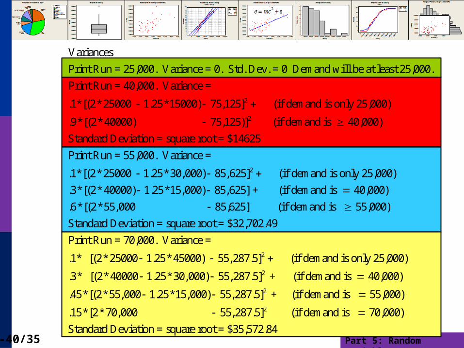
Variances
Print Run = 25,000. Variance = 0. Std. Dev. = 0 Demand will be at least 25,000.
Print Run
.1*[(2*25000 1.25*15000) 75,125] (if demand is o
= 40,000.
nly 25,000)
Va
.
rian
9*[(2*4000
ce =
0
2
2
(if demand is 40,000)
Standard Deviation = square root = $14625
Print Run = 55,000. Variance
) 75,125)]
.1*[(2*25000 1.25*30,000) 85,625] (if demand is only
=
25,0
+ (if demand is 40,000)
.6*[(2*55,000 85,625] (if demand is 55,000)
Standard Dev
00)
.3*[(2*40000) 1.25*15,00
iation = square root = $32
0) 85,625]
,702.49
2
2
.1* [(2*25000 1.25*45000) 55,287.5] (if demand is only 25,000)
.3* [
Run = 70,000. Variance =
+ (if demand is 40,000)
.4
(2*40000 1.25*30,000) 55,287.5]
1.25*15,000) 55,287.5*[(2*55,0 0 50
2
2
]
55,287.5
+ (if demand is 55,000)
.15*[2*70,000 (if demand is 70,000)
Standard Deviation = square root = $35,57 .84
]
2
Part 5: Random Variables5-41/35
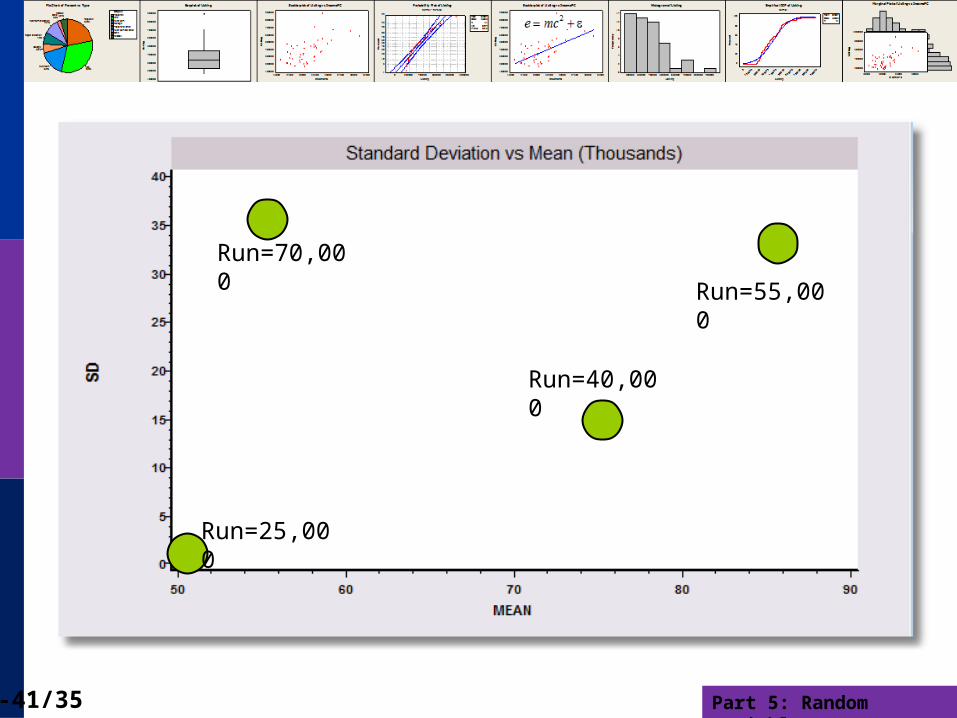
Run=25,000
Run=70,000
Run=40,000
Run=55,000
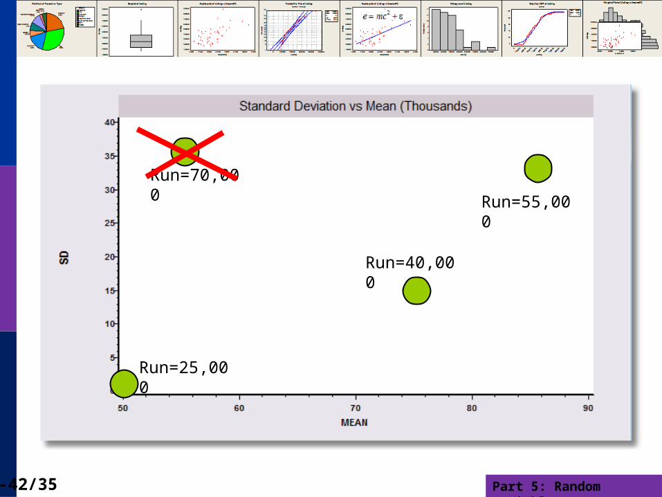
Part 5: Random Variables5-42/35
Run=25,000
Run=70,000
Run=40,000
Run=55,000
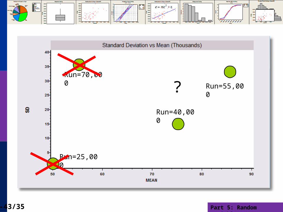
Part 5: Random Variables5-43/35
Run=25,000
Run=70,000
Run=40,000
Run=55,000?