part 10: central limit theorem 10-1/48 statistics and data analysis professor william greene stern...

Part 10: Central Limit Theorem10-1/48

Statistics and Data Analysis

Professor William Greene

Stern School of Business

IOMS Department

Department of Economics


Statistics and Data Analysis

Part 10 – The Law of Large Numbers and the Central Limit Theorem


Sample Means and the Central Limit Theorem

Statistical Inference: Drawing Conclusions from Data Sampling

Random sampling Biases in sampling Sampling from a particular distribution

Sample statistics Sampling distributions

Distribution of the mean More general results on sampling distributions

Results for sampling and sample statistics The Law of Large Numbers The Central Limit Theorem


Measurement as Description

Population

MeasurementCharacteristicsBehavior PatternsChoices and DecisionsMeasurementsCounts of Events

Sessions 1 and 2: Data Description

Numerical (Means, Medians, etc.)

Graphical

No organizing principles: Where did the data come from? What is the underlying process?


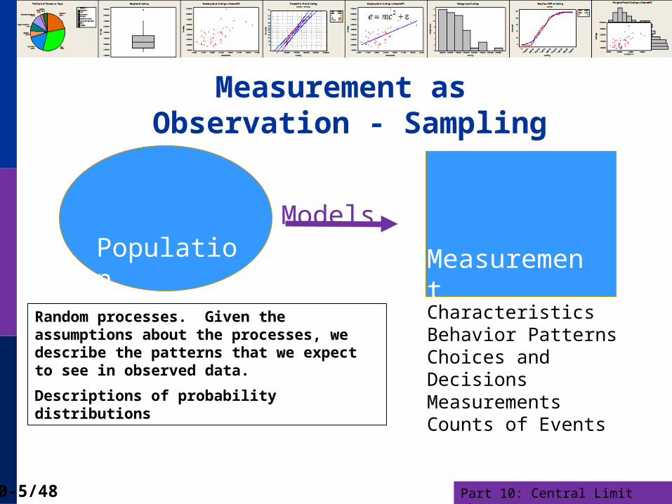
Measurement as Observation - Sampling

Population

Measurement

Models

CharacteristicsBehavior PatternsChoices and DecisionsMeasurementsCounts of Events

Random processes. Given the assumptions about the processes, we describe the patterns that we expect to see in observed data.

Descriptions of probability distributions


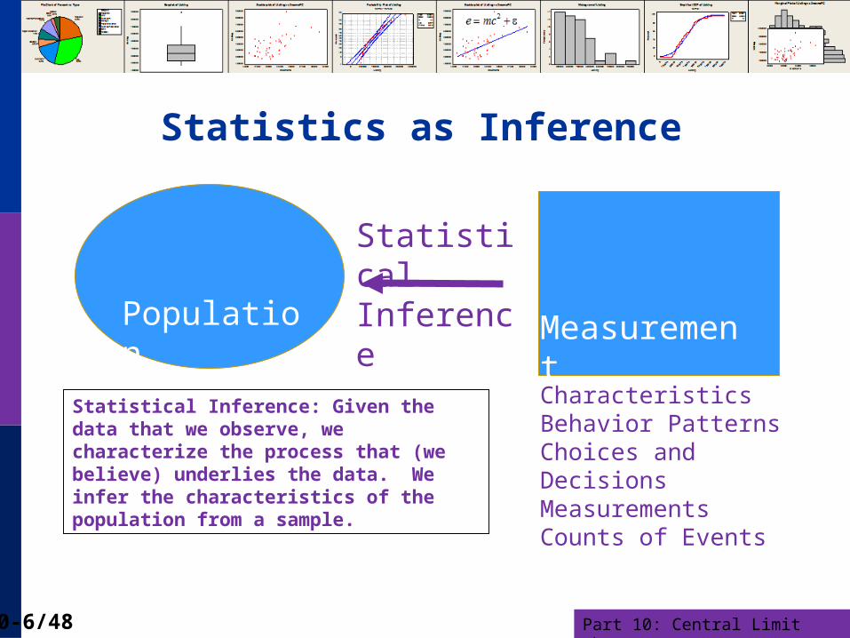
Statistics as Inference

Population

MeasurementCharacteristicsBehavior PatternsChoices and DecisionsMeasurementsCounts of Events

Statistical Inference

Statistical Inference: Given the data that we observe, we characterize the process that (we believe) underlies the data. We infer the characteristics of the population from a sample.


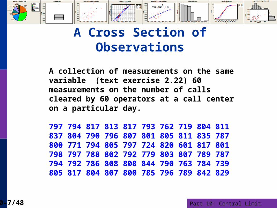
A Cross Section of Observations

A collection of measurements on the same variable (text exercise 2.22) 60 measurements on the number of calls cleared by 60 operators at a call center on a particular day.

797 794 817 813 817 793 762 719 804 811 837 804 790 796 807 801 805 811 835 787800 771 794 805 797 724 820 601 817 801798 797 788 802 792 779 803 807 789 787794 792 786 808 808 844 790 763 784 739805 817 804 807 800 785 796 789 842 829


Random Sampling

What makes a sample a random sample? Independent observations Same underlying process generates each

observation made

Population

The set of all possible observations that could be drawn in a sample


Overriding Principles in Statistical Inference

Characteristics of a random sample will mimic (resemble) those of the population Mean, Median, etc. Histogram

The sample is not a perfect picture of the population.

It gets better as the sample gets larger.


“Representative Opinion Polling” and Random Sampling


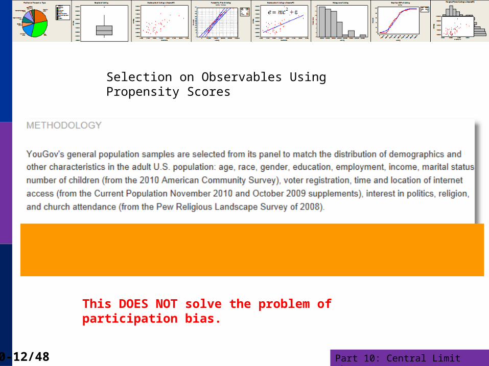
Selection on Observables Using Propensity Scores

This DOES NOT solve the problem of participation bias.


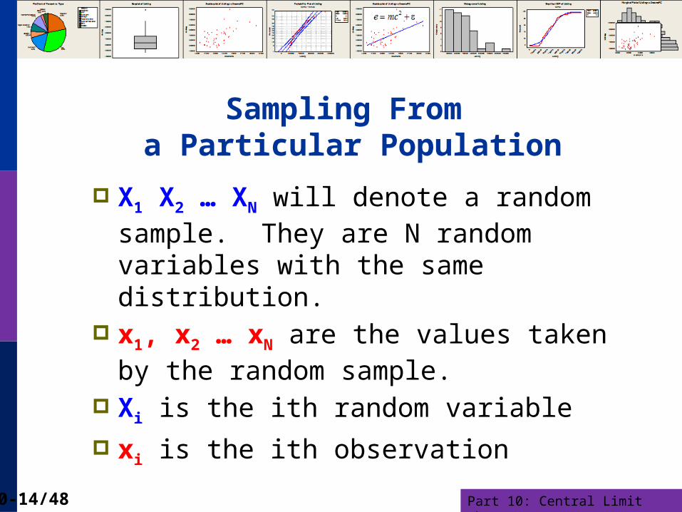
Sampling From a Particular Population

X1 X2 … XN will denote a random sample. They are N random variables with the same distribution.

x1, x2 … xN are the values taken by the random sample.

Xi is the ith random variable

xi is the ith observation


Sampling from a Poisson Population

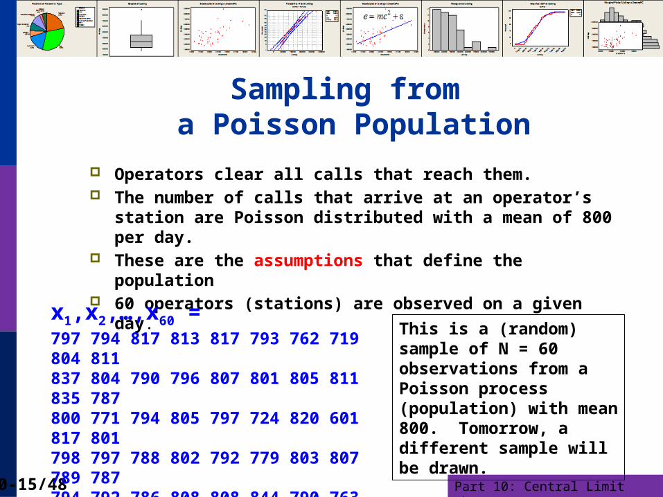
Operators clear all calls that reach them. The number of calls that arrive at an operator’s station are

Poisson distributed with a mean of 800 per day. These are the assumptions that define the population 60 operators (stations) are observed on a given day.

x1,x2,…,x60 = 797 794 817 813 817 793 762 719 804 811 837 804 790 796 807 801 805 811 835 787800 771 794 805 797 724 820 601 817 801798 797 788 802 792 779 803 807 789 787794 792 786 808 808 844 790 763 784 739805 817 804 807 800 785 796 789 842 829

This is a (random) sample of N = 60 observations from a Poisson process (population) with mean 800. Tomorrow, a different sample will be drawn.


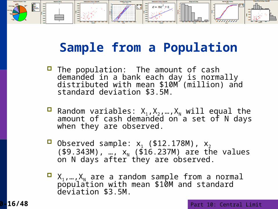
Sample from a Population

The population: The amount of cash demanded in a bank each day is normally distributed with mean $10M (million) and standard deviation $3.5M.

Random variables: X1,X2,…,XN will equal the amount of cash demanded on a set of N days when they are observed.

Observed sample: x1 ($12.178M), x2 ($9.343M), …, xN ($16.237M) are the values on N days after they are observed.

X1,…,XN are a random sample from a normal population with mean $10M and standard deviation $3.5M.


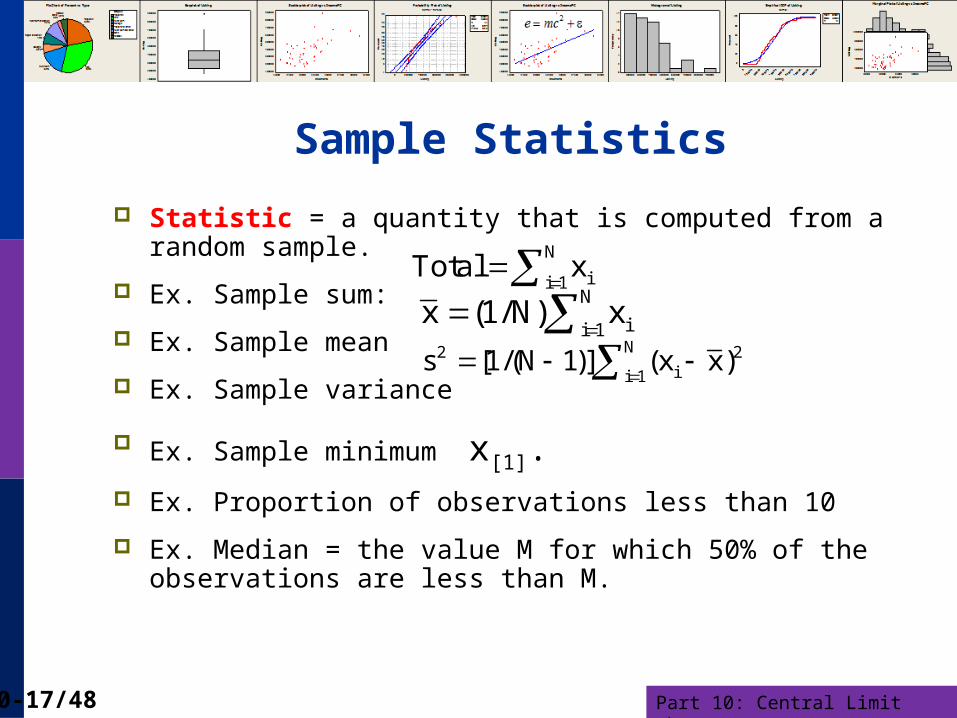
Sample Statistics

Statistic = a quantity that is computed from a random sample.

Ex. Sample sum:

Ex. Sample mean

Ex. Sample variance

Ex. Sample minimum x[1]. Ex. Proportion of observations less than 10

Ex. Median = the value M for which 50% of the observations are less than M.

N

ii 1Total x

N

ii 1x (1/N) x

N2 2

ii 1s [1/(N 1)] (x x)


Sampling Distribution

The sample is itself random, since each member is random. (A second sample will differ randomly from the first one.)

Statistics computed from random samples will vary as well.


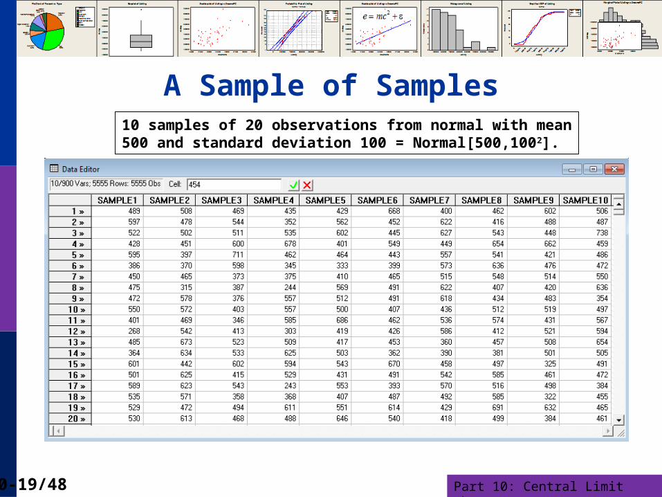
A Sample of Samples10 samples of 20 observations from normal with mean 500 and standard deviation 100 = Normal[500,1002].


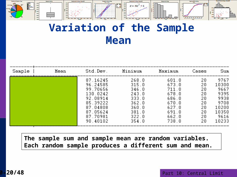
Variation of the Sample Mean

The sample sum and sample mean are random variables. Each random sample produces a different sum and mean.


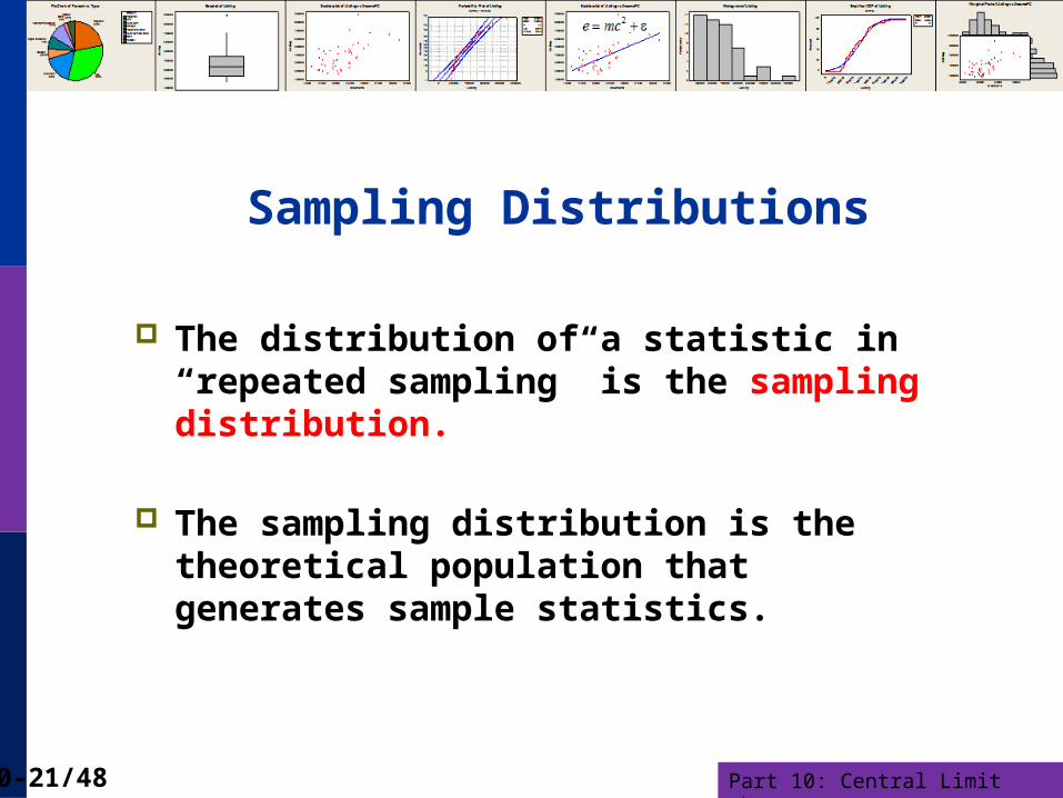
Sampling Distributions

The distribution of a statistic in “repeated sampling” is the sampling distribution.

The sampling distribution is the theoretical population that generates sample statistics.


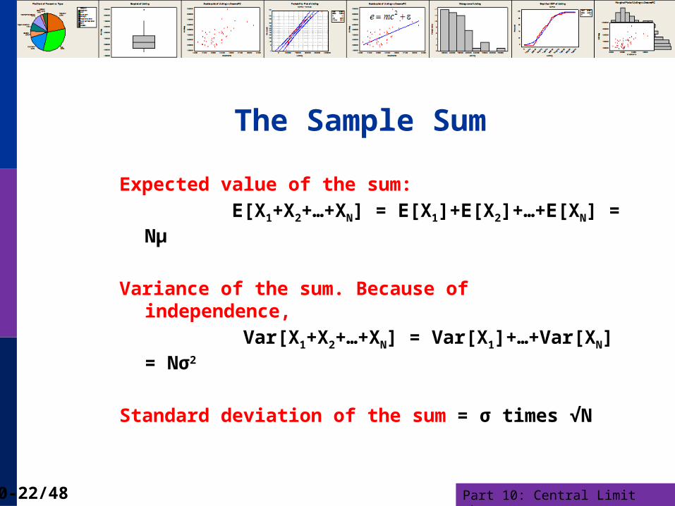
The Sample Sum

Expected value of the sum:

E[X1+X2+…+XN] = E[X1]+E[X2]+…+E[XN] = Nμ

Variance of the sum. Because of independence,

Var[X1+X2+…+XN] = Var[X1]+…+Var[XN] = Nσ2

Standard deviation of the sum = σ times √N


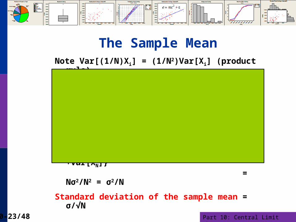
The Sample MeanNote Var[(1/N)Xi] = (1/N2)Var[Xi] (product rule)

Expected value of the sample mean

E(1/N)[X1+X2+…+XN] = (1/N){E[X1]+E[X2]+…+E[XN]} = (1/N)Nμ = μ

Variance of the sample mean

Var(1/N)[X1+X2+…+XN] = (1/N2){Var[X1]+…+Var[XN]} = Nσ2/N2 = σ2/N

Standard deviation of the sample mean = σ/√N


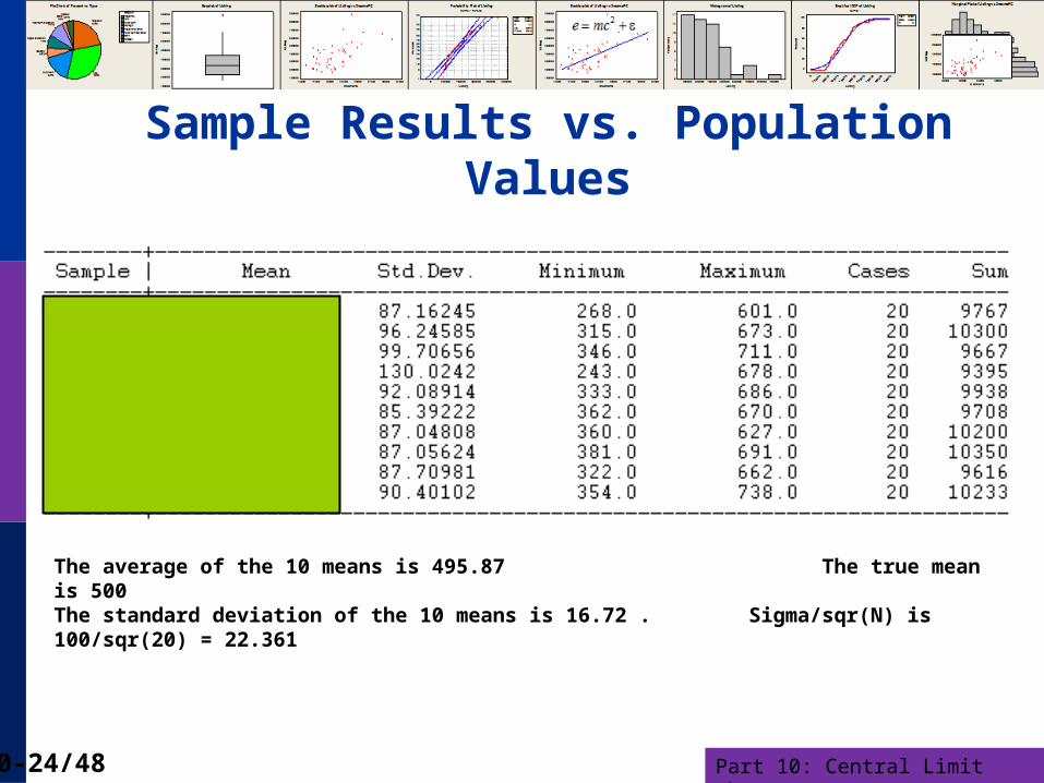
Sample Results vs. Population Values

The average of the 10 means is 495.87 The true mean is 500The standard deviation of the 10 means is 16.72 . Sigma/sqr(N) is 100/sqr(20) = 22.361


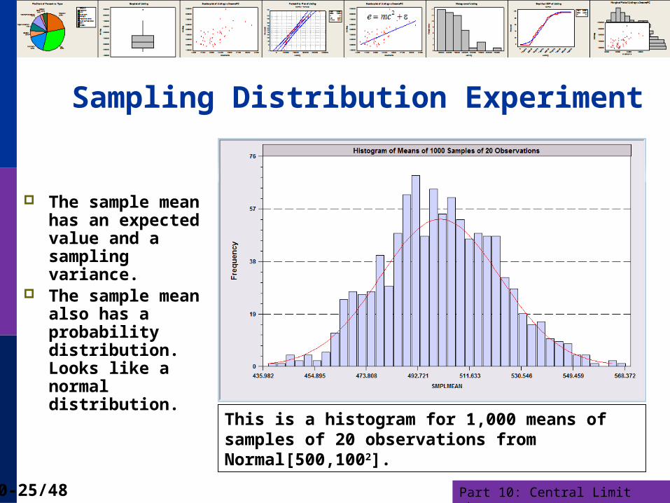
Sampling Distribution Experiment

The sample mean has an expected value and a sampling variance.

The sample mean also has a probability distribution. Looks like a normal distribution.

This is a histogram for 1,000 means of samples of 20 observations from Normal[500,1002].


The Distribution of the Mean

Note the resemblance of the histogram to a normal distribution.

In random sampling from a normal population with mean μ and variance σ2, the sample mean will also have a normal distribution with mean μ and variance σ2/N.

Does this work for other distributions, such as Poisson and Binomial? Yes. The mean is approximately normally distributed.


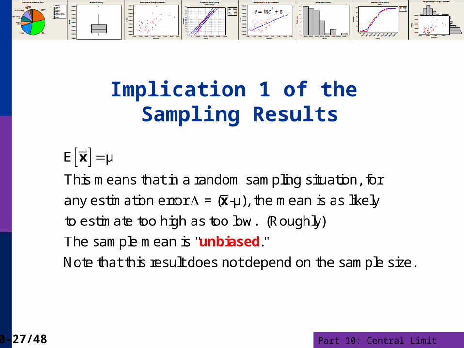
Implication 1 of the Sampling Results

E μ

This means that in a random sampling situation, for

any estimation error = ( -μ), the mean is as likely

to estimate too high as too low. (Roughly)

The sample mean is " ."

Note that this resu

unbiased

x

x

lt does not depend on the sample size.


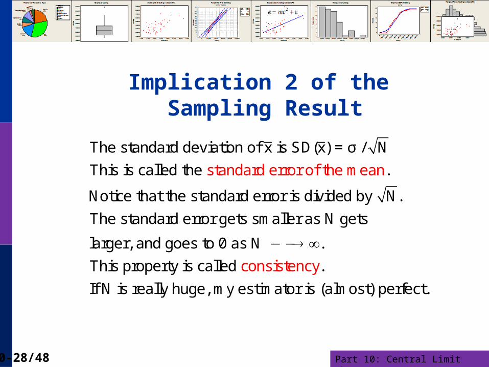
Implication 2 of the Sampling Result

The standard deviation of x is SD(x) = σ / N

This is called the .

Notice that the standard error is divided by N.

The standard error gets smaller as N get

standard

s

larger,

erro

and

r of the m

goes to

ean

0 as N .

This property is called .

If N is really huge, my estimator is (al

consistency

most) perfect.


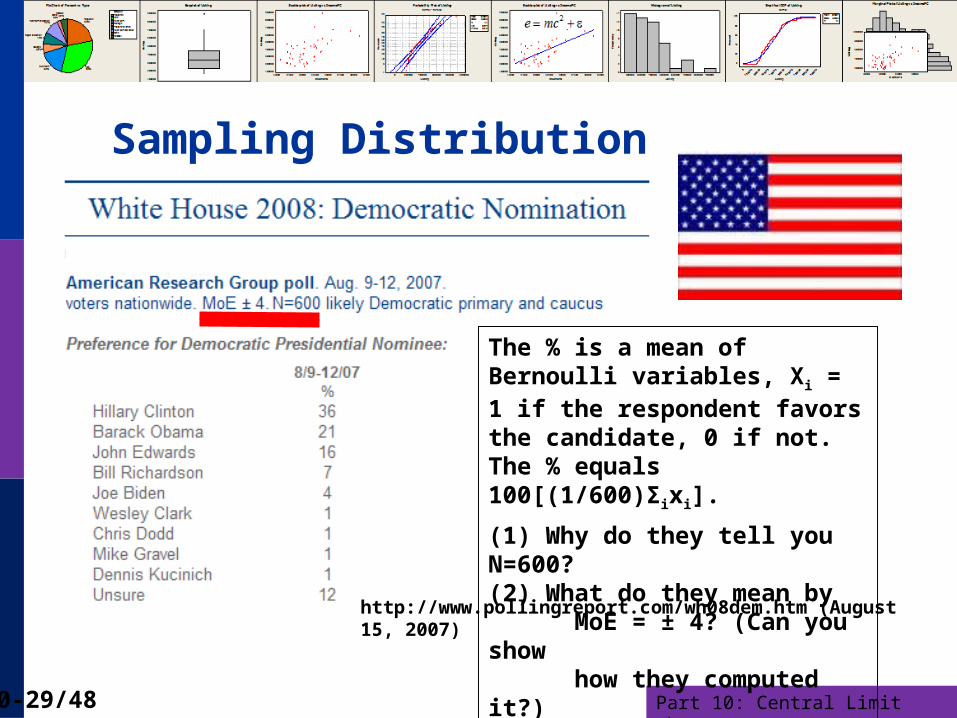
Sampling Distribution

The % is a mean of Bernoulli variables, Xi = 1 if the respondent favors the candidate, 0 if not. The % equals 100[(1/600)Σixi].

(1) Why do they tell you N=600?(2) What do they mean by MoE = ± 4? (Can you show how they computed it?)

http://www.pollingreport.com/wh08dem.htm (August 15, 2007)


Two Major Theorems

Law of Large Numbers: As the sample size gets larger, sample statistics get ever closer to the population characteristics

Central Limit Theorem: Sample statistics computed from means (such as the means, themselves) are approximately normally distributed, regardless of the parent distribution.


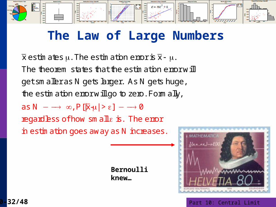
The Law of Large Numbers

x estimates . The estimation error is x .

The theorem states that the estimation error will

get smaller as N gets larger. As N gets huge,

the estimation error will go to zero. Formal

as N

ly,

, P[|

x- | > ] 0

regardless of how small is. The error

in estimation goes away as N increases.

Bernoulli knew…


The Law of Large Numbers: Example

Event consists of two random outcomes YES and NOProb[YES occurs] = θ θ need not be 1/2Prob[NO occurs ] = 1- θEvent is to be staged N times, independently

N1 = number of times YES occurs, P = N1/N

LLN: As N Prob[(P - θ) > ] 0 no matter how small is.

For any N, P will deviate from θ because of randomness.As N gets larger, the difference will disappear.


The LLN at Work – Roulette WheelProportion of Times 2,4,6,8,10 Occurs

I

.1

.2

.3

.4

.5

.0100 200 300 400 5000

P1I

Computer simulation of a roulette wheel – θ = 5/38 = 0.1316P = the proportion of times (2,4,6,8,10) occurred.


Application of the LLN

The casino business is nothing more than a huge application of the law of large numbers. The insurance business is close to this as well.


Insurance Industry* and the LLN Insurance is a complicated business. One simple theorem drives the entire industry

Insurance is sold to the N members of a ‘pool’ of purchasers, any one of which may experience the ‘adverse event’ being insured against.

P = ‘premium’ = the price of the insurance against the adverse event F = ‘payout’ = the amount that is paid if the adverse event occurs = the probability that a member of the pool will experience the adverse event. The expected profit to the insurance company is N[P - F] Theory about and P. The company sets P based on . If P is set too high, the

company will make lots of money, but competition will drive rates down. (Think Progressive advertisements.) If P is set to low, the company loses money.

How does the company learn what is? What if changes over time. How does the company find out? The Insurance company relies on (1) a large N and (2) the law of

large numbers to answer these questions.

* See course outline session 4: Credit Default Swaps


Insurance Industry Woes

Adverse selection: Price P is set for which is an average over the population – people have very different s. But, when the insurance is actually offered, only people with high buy it. (We need young healthy people to sign up for insurance.)

Moral hazard: is ‘endogenous.’ Behavior changes because individuals have insurance. (That is the huge problem with fee for service reimbursement. There is an incentive to overuse the system.)


Implication of the Law of Large Numbers

If the sample is large enough, the difference between the sample mean and the true mean will be trivial.

This follows from the fact that the variance of the mean is σ2/N → 0.

An estimate of the population mean based on a large(er) sample is better than an estimate based on a small(er) one.


Implication of the LLN

Now, the problem of a “biased” sample: As the sample size grows, a biased sample produces a better and better estimator of the wrong quantity.

Drawing a bigger sample does not make the bias go away. That was the essential fallacy of the Literary Digest poll and of the Hite Report.


3000 !!!!!

Or is it 100,000?


Central Limit Theorem

Theorem (loosely): Regardless of the underlying distribution of the sample observations, if the sample is sufficiently large (generally > 30), the sample mean will be approximately normally distributed with mean μ and standard deviation σ/√N.


Implication of the Central Limit Theorem

Inferences about probabilities of eventsbased on the sample mean can use thenormal approximation even if the datathemselves are not drawn from a normalpopulation.


PoissonSample

797 794 817 813 817 793 762 719 804 811 837 804 790 796 807 801 805 811 835 787800 771 794 805 797 724 820 601 817 801798 797 788 802 792 779 803 807 789 787794 792 786 808 808 844 790 763 784 739805 817 804 807 800 785 796 789 842 829

The sample of 60 operators from text exercise 2.22 appears above. Suppose it is claimed that the population that generated these data is Poisson with mean 800 (as assumed earlier). How likely is it to have observed these data if the claim is true?

The sample mean is 793.23. The assumed population standard error of the mean, as we saw earlier, is sqr(800/60) = 3.65. If the mean really were 800 (and the standard deviation were 28.28), then the probability of observing a sample mean this low would be

P[z < (793.23 – 800)/3.65] = P[z < -1.855] = .0317981.

This is fairly small. (Less than the usual 5% considered reasonable.) This might cast some doubt on the claim.


Applying the CLT

The population is believed to be Poisson with mean (and variance)

equal to 800. A sample of 60 is drawn. Management has decided

that if the sample of 60 produces a mean less than or equal to

790, then it will be necessary to upgrade the switching machinery.

What is the probability that they will erroneously conclude that the

performance of the operators has degraded?

The question asks for P[x < 790]. The population σ is 800 = 28.28.

Thus, the standard error of the mean is 28.28/ 60 = 3.65. The

790-800probability is P z p[z -2.739] = 0.0030813. (Unlikely)

3.65


Overriding Principle in Statistical Inference

(Remember) Characteristics of a random sample will mimic (resemble) those of the population

Histogram Mean and standard deviation The distribution of the observations.


Using the Overall Result in This Session

A sample mean of the response times in 911 calls is computed from N events.

How reliable is this estimate of the true average response time?

How can this reliability be measured?


Question on Midterm: 10 Points

The central principle of classical statistics (what we are studying in this course), is that the characteristics of a random sample resemble the characteristics of the population from which the sample is drawn. Explain this principle in a single, short, carefully worded paragraph. (Not more than 55 words. This question has exactly fifty five words.)


Summary

Random Sampling Statistics Sampling Distributions Law of Large Numbers Central Limit Theorem

part 10: central limit theorem 10-1/48 statistics and data analysis professor william greene stern...

Documents

central limit theorem

sample slide

sampling sampling

random sampling slide

random sample

sampling distributions

observed data

decisions measurements