part a simulation - oxford statisticswinkel/asim11.pdfpart a simulation matthias winkel department...

Part A

Simulation

Matthias WinkelDepartment of Statistics

University of Oxford

These notes benefitted from the TT 2010 notes by Geoff Nicholls.

TT 2011

Part A

SimulationMatthias Winkel – 8 lectures TT 2011

Prerequisites

Part A Probability and Mods Statistics

Aims

This course introduces Monte Carlo methods, collectively one of the most importantanalytical tools of modern Statistical Inference.

Synopsis

Motivation. Inversion. Transformation methods.Rejection.Variance reduction via Importance sampling.The Metropolis algorithm (finite space), reversibility, ergodicity.Applications: conditioned and extreme events, likelihood and missing data, samplinguniformly at random.

Problem sheets in classes will include a separate section with some examples of simulationusing R.

Reading

S. M. Ross: Simulation. Elsevier, 4th edition, 2006J. R. Norris: Markov chains. CUP, 1997C. P. Robert and G. Casella: Monte Carlo Statistical Methods. Springer, 2004B. D. Ripley: Stochastic Simulation. Wiley, 1987

Contents

1 Introduction 1

1.1 Motivation . . . . . . . . . . . . . . . . . . . . . . . . . . . . . . . . . . . 1

1.2 Overview . . . . . . . . . . . . . . . . . . . . . . . . . . . . . . . . . . . . 2

1.3 Structure of the course . . . . . . . . . . . . . . . . . . . . . . . . . . . . 6

2 Inversion and transformation methods 7

2.1 The inversion method . . . . . . . . . . . . . . . . . . . . . . . . . . . . . 7

2.2 The transformation method . . . . . . . . . . . . . . . . . . . . . . . . . 9

3 The rejection method 11

3.1 Simulating from probability density functions? . . . . . . . . . . . . . . . 11

3.2 Conditioning by repeated trials . . . . . . . . . . . . . . . . . . . . . . . 12

3.3 Rejection . . . . . . . . . . . . . . . . . . . . . . . . . . . . . . . . . . . 13

4 Refining simulation methods 15

4.1 More rejection . . . . . . . . . . . . . . . . . . . . . . . . . . . . . . . . . 15

4.2 Random permutations . . . . . . . . . . . . . . . . . . . . . . . . . . . . 16

4.3 Discrete distributions and random parameters . . . . . . . . . . . . . . . 17

5 Importance sampling 19

5.1 Monte-Carlo integration . . . . . . . . . . . . . . . . . . . . . . . . . . . 19

5.2 Variance reduction via importance sampling . . . . . . . . . . . . . . . . 21

5.3 Example: Importance sampling for Normal tails . . . . . . . . . . . . . . 22

6 Markov chain Monte-Carlo 25

6.1 Simulation of Markov chains . . . . . . . . . . . . . . . . . . . . . . . . . 25

6.2 Monte-Carlo algorithm . . . . . . . . . . . . . . . . . . . . . . . . . . . . 26

6.3 Reversible Markov chains . . . . . . . . . . . . . . . . . . . . . . . . . . . 28

6.4 The Metropolis-Hastings algorithm . . . . . . . . . . . . . . . . . . . . . 28

7 The Metropolis-Hastings algorithm 29

7.1 The basic Metropolis-Hastings algorithm . . . . . . . . . . . . . . . . . . 29

7.2 The Metropolis-Hastings algorithm in a more general setting . . . . . . . 31

7.3 Example: the Ising model . . . . . . . . . . . . . . . . . . . . . . . . . . 32

v

vi Contents

8 Unknown normalisation constants 378.1 Normalisation constants . . . . . . . . . . . . . . . . . . . . . . . . . . . 378.2 Rejection method . . . . . . . . . . . . . . . . . . . . . . . . . . . . . . . 388.3 Importance sampling . . . . . . . . . . . . . . . . . . . . . . . . . . . . . 388.4 Metropolis-Hastings algorithm . . . . . . . . . . . . . . . . . . . . . . . . 408.5 Conclusion . . . . . . . . . . . . . . . . . . . . . . . . . . . . . . . . . . . 40

A Assignments IA.1 Inversion, transformation and rejection . . . . . . . . . . . . . . . . . . . IIIA.2 Rejection and importance sampling . . . . . . . . . . . . . . . . . . . . . VA.3 Importance sampling and MCMC . . . . . . . . . . . . . . . . . . . . . . VII

B Solutions IXB.1 Inversion, transformation and rejection . . . . . . . . . . . . . . . . . . . IXB.2 Rejection and importance sampling . . . . . . . . . . . . . . . . . . . . . XIIIB.3 Importance sampling and MCMC . . . . . . . . . . . . . . . . . . . . . . XVII

C Solutions to optional R questions XXIC.1 Inversion, transformation and rejection . . . . . . . . . . . . . . . . . . . XXIC.3 Importance sampling and MCMC . . . . . . . . . . . . . . . . . . . . . . XXIV

Lecture 1

Introduction

Reading: Ross Chapters 1 and 3Further reading: Ripley Chapters 1, and 2 (25 years old, but the caveat is instructive)

1.1 Motivation

The aim of this section is to give brief reasons why simulation is useful and why mathe-maticians and statisticians should be interested in simulation. To focus ideas, we beginby an example and an attempt at defining what simulation is.

Example 1 Ross’s book starts by considering an example of a pharmacist filling pre-scriptions. At a qualitative level, customers arrive and queue to be served. Their pre-scriptions require varying amounts of service time. The pharmacist cares about bothcustomer satisfaction and not excessively exceeding his 9am-5pm working day.

A mathematical approach to the problem is to set up stochastic models for the arrivalprocess of customers and for the service times, calibrated based on past experience. Oneof the most popular models is to consider independent exponentially distributed inter-arrival and service times, with certain service and inter-arrival parameters. This model isanalytically tractable (see Part B Applied Probability), but it is only a first approximationof reality. We want to model varying arrival intensities and non-exponential service timesthat may interact with quantities such as the number of people in the queue.

Let us focus on a specific question. If the pharmacist continues to deal with allcustomers in the pharmacy at 5pm but no more new customers, what proportion of dayswill he finish after 5.30pm? Once a precise model has been formulated, a computer cansimulate many days of customers and compute the proportion of simulated days he wouldfinish after 5.30pm, a Monte-Carlo average approximating the model answer, which willbe close to the real answer if our model is sufficiently realistic.

Simulation is a subject that can be studied in different ways and with different aims.As a mathematical subject, the starting point is often a sequence of independent randomvariables (Uk, k ≥ 1) that are uniformly distributed on the interval (0, 1); notation:Uk ∼ Unif(0, 1). The aim of the game is to generate from these uniform random variablesmore complicated random variables and stochastic models. From an algorithmic point

1

2 Lecture Notes – Part A Simulation – Oxford TT 2011

of view, the efficiency of such generation of random variables can be analysed. Theimplementation of efficient algorithms makes simulation useful to applied disciplines.

The most basic use in applied or indeed theoretical disciplines is to repeatedly andindependently observe realisations of a stochastic model, which on the one hand can becompared with and related to real world systems and on the other hand can give rise toconjectures about the stochastic model itself that can then be approached mathematically.A fundamental feature of mathematical modelling is the trade-off between proximityto the real world and (analytic) tractability. Simulation methods allow to gain moreproximity to the real world while keeping (computational) tractability. The complexity ofthe stochastic model often poses some challenges. More specific uses of simulation includethe calibration of parameters in a complex system to control the failure probability orthe approximation of critical values for a statistical test where the distribution of the teststatistic is not explicit. Simulation then becomes a tool to help with decision making.

In this course, you will see some implementation in the statistical computing packageR for illustration purposes and to help your intuition. The main focus however is onsome key mathematical techniques building on Part A Probability and Mods Statistics.Indeed, simulation allows to illustrate notions and results from those courses that enhanceunderstanding of the material of those courses.

1.2 Overview

Consider a sequence of independent Unif(0, 1) random variables (Uk, k ≥ 1). In R, anynumber n of these can be generated by the command runif(n). Figure 1.1 shows twoplots of, respectively 20 and 1,000,000 uniform random variables in a histogram. In thefirst histogram, the actual realisations of uniform variables have been added betweenthe bars and the x-axis. Note the substantial deviation from bars of equal height dueto randomness in sampling. This effect disappears as the number of variables tends toinfinity – this is essentially a consequence of the (Strong) Law of Large Numbers, whichimplies that the proportion in each of the 20 boxes converges to 1/20 almost surely. Moregenerally, the Glivenko-Cantelli theorem shows that empirical cumulative distributionfunctions converge uniformly to the underlying cumulative distribution function.

R code:

x<-runif(20)

hist(x)

x<-runif(1000000)

hist(x)

Figure 1.1: Histograms of Unif(0, 1), resp. n = 20 and n = 1, 000, 000, with R code.

Lecture 1: Introduction 3

Strictly speaking, any computer will generate at best pseudo-random numbers (deter-ministic, but apparently random), the question of what actual random numbers are hasa deep philosophical dimension. While the mathematical theory (based on Kolmogorov’saxioms) is sound, the interface with the real world, also computers, is problematic.

However, the behaviour of random numbers generated by modern random numbergenerators (whose construction is based on number theory Nk+1 = (aNk + c) mod m forsuitable a, c, m, then Uk+1 = Nk+1/(m + 1), e.g. m = 219937 − 1 as the default in R),resembles mathematical random numbers in many respects. In particular, standard testsfor uniformity, independence etc. do not show significant deviations. We will not go intoany more detail of the topics touched upon here and refer the reader to the literature.

The following examples introduce some important ideas to dwell on and they collec-tively give an overview of the course.

Example 2 For independent U1, U2 ∼ Unif(0, 1), the pair (U1, U2) has bivariate uniformdistribution on (0, 1)2; the variable V1 = a + (b − a)U1 is uniformly distributed on (a, b)with density 1/(b − a) on (a, b); the pair (V1, V2) = (a + (b − a)U1, c + (d − c)U2) isuniformly distributed on (a, b)× (c, d). This is an example of the transformation method,here, linear transformation. Non-linear transformations give non-uniform distributions,in general. For example, W1 = − ln(1 − U1) ∼ Exp(1), since

F (w) = P(W1 ≤ w) = P(− ln(1 − U1) ≤ w) = P(U1 ≤ 1 − e−w) = 1 − e−w, w ≥ 0.

Note that F−1(u) = − ln(1−u), u ∈ [0, 1), is the inverse cumulative distribution function.Setting W1 = F−1(U1) is an instance of the inversion method.

Discrete uniform distributions can be obtained as Z1 = [nU1] where [·] denotes theinteger part function:

P([nU1] = j) = P(j ≤ nU1 < j + 1) = P(U1 ∈ [j/n, (j + 1)/n)) = 1/n, j = 0, . . . , n− 1.

Example 3 Uniform distributions on subsets A ⊂ [a, b]× [c, d] can be obtained via con-ditioning: conditionally given that (V1, V2) ∈ A, the pair (V1, V2) is uniformly distributed

on A. Intuitively, if we repeat simulating (V(k)1 , V

(k)2 ) until we get (V

(k)1 , V

(k)2 ) ∈ A, the

resulting (V1, V2) = (V(k)1 , V

(k)2 ) is uniformly distributed on A.

Let us formulate a specific example in pseudo-code, i.e. phrases close to computercode that are easily implemented, but using fuller sentence structure:

1. Generate two independent random numbers U1 ∼ Unif(0, 1) and U2 ∼ Unif(0, 1).

2. If U21 + U2

2 < 1, go to 3., else go to 1.

3. Return the vector (U1, U2).

This algorithm simulates a uniform variable in the quarter disk. This is an example ofthe rejection method. Analogously for a uniform distribution on A = [0, 1]2 ∪ [1, 2]2:

1. Generate two independent random numbers U1 ∼ Unif(0, 1) and U2 ∼ Unif(0, 1).

2. Set (V1, V2) = (2U1, 2U2). If (V1, V2) ∈ A, go to 3., else go to 1.

3. Return the vector (V1, V2).


Note that (V1, V2) has marginal distributions V1, V2 ∼ Unif(0, 2), but V1 and V2 are notindependent. Generating dependent random variables from independent ones is not justuseful in simulation, but also in measure-theoretic probability/integration, where the firststep is the existence of Lebesgue measure on [0, 1], the next steps Lebesgue measure onfinite products [0, 1]n and infinite products [0, 1]N. Product measures reflect independenceand can be transformed/restricted to get measures with dependent marginals.

Example 4 Sometimes we do not need the exact distribution of a random variable X,but only a tail probability P(X > c) or an expectation E(X) or E(f(X)). We could usethe (Strong) Law of Large Numbers on independent copies Xj of X to approximate

X1 + · · · + Xn

n→ E(X) “almost surely” (strengthens “in probability”) as n → ∞.

This result holds as soon as E(|X|) < ∞. We can always apply it to random variables

Yj = 1Xj>c =

1 if Xj > c,0 otherwise,

and to Zj = f(Xj) if E(|Z|) = E(|f(X)|) < ∞. This method is often not very efficient,particularly if c is large or f is small for most, but not all possible values of X. Importancesampling boosts the number and compensates the weight of “relevant” realisations of X.

Example 5 The normal distribution is the limit in the Central Limit Theorem (CLT):

Zn =U1 + · · · + Un − n/2√

n/12→ Normal(0, 1), in distribution, as n → ∞,

so for large n, the approximating Zn will be almost normally distributed, see Figure1.2. The case n = 12 used to be popular, but is not accurate, and larger n are lessefficient. But, we can similarly use the Markov chain convergence and ergodic theoremsto approximate stationary distributions of Markov chains. Example: for a graph (V, E),consider the random walk on V , where each step is to a neighbouring vertex chosenuniformly at random. A much more general example is the Metropolis-Hastings algorithm.

R code:

n<-100

k<-10000

U<-runif(n*k)

M<-matrix(U,n,k)

X<-apply(M,2,’sum’)

Z<-(X-n/2)/sqrt(n/12)

hist(Z)

qqnorm(Z)

Figure 1.2: Histogram and Q-Q plot of k = 10, 000 Normal(0, 1) via CLT for n = 100.

Lecture 1: Introduction 5

We can actually investigate the quality of approximation, when we “apply” the CLTfor small values of n. See Figure 1.3, which uses the same code as Figure 1.2, just forn = 1, n = 2, n = 3 and n = 5. We see that the approximation, which starts withuniform and triangular distributions for n = 1 and n = 2 becomes quite good (at thisgraphical level) for n = 5, and further improves in the tails for n = 10 and n = 100.

Figure 1.3: Histogram, Q-Q plot of k = 10, 000 Normal(0, 1) for n = 1, 2, 3, 5, 10, 100.


1.3 Structure of the course

We will now go back to the simulation of real-valued and multivariate (mostly bivariate)random variables. Lecture 2 will treat the inversion method to simulate general one-dimensional distributions and the transformation method as a generalisation to deal withthe multivariate case. Lecture 3 will discuss the rejection method and some more examplescombining rejection and transformation. Most exercises for this material will be onAssignment 1.

Lectures 4 and 5 will refine the rejection method to deal with importance sampling,Assignment 2. This leaves Lectures 6-8 for the Metropolis-Hastings algorithm and moreabout Markov chain Monte-Carlo (MCMC) and applications, Assignment 3.

Lecture 2

Inversion and transformationmethods

Reading: Robert and Casella Sections 2.1 and 2.2, Ross Section 5.1Further reading: Ripley Chapter 3

2.1 The inversion method

Recall that a function F : R → [0, 1] is a cumulative distribution function if

• F is increasing, i.e. x ≤ y ⇒ F (x) ≤ F (y);

• F is right-continuous, i.e. F (x + ε) → F (x) as ε ↓ 0;

• F (x) → 0 as x → −∞;

• and F (x) → 1 as x → ∞.

A random variable X : Ω → R has cumulative distribution function F if P(X ≤ x) = F (x)for all x ∈ R. This implies

• P(X ∈ (a, b]) = F (b) − F (a), P(X ∈ [a, b]) = F (b) − F (a−), P(X ∈ (a, b)) =F (b−) − F (a) etc., where F (a−) = limε↓0 F (a − ε). In particular, P(X = a) =F (a) − F (a−) > 0 iff F jumps at a.

• If F is differentiable on R, with derivative f , then X is continuously distributedwith probability density function f .

If F : R → (0, 1) is a continuous and strictly increasing cumulative distribution function,we can define its inverse F−1 : (0, 1) → R.

Proposition 6 (Inversion) If F : R → (0, 1) is a continuous and strictly increasing cu-mulative distribution function with inverse F−1, then F−1(U) has cumulative distributionfunction F , if U ∼ Unif(0, 1).

In fact, this result holds for every cumulative distribution function, provided we appropri-ately define F−1(u). We will explore this on the first assignment sheet, see also Example8 below.

7


Proof: Let x ∈ R. Since F and F−1 are strictly monotonic increasing, application of For F−1 preserves inequalities, and so

P(F−1(U) ≤ x) = P(U ≤ F (x)) = F (x).

Since this holds for all x ∈ R, F−1(U) has cumulative distribution function F . 2

This is useful only if we have the inverse cumulative distribution function at our dis-posal. This is not usually the case, but it includes the case for the exponential distributionand more generally for the Weibull distribution. If we slightly modify the proposition toapply to strictly increasing continuous functions F : [0,∞) → [0, 1) with F (0) = 0 andF (x) → 1 as x → ∞, the proof still applies (but as we have said it actually holds in fullgenerality):

Example 7 (Weibull) Let α, λ ∈ (0,∞). The distribution with survival function

F (x) = 1 − F (x) = exp (−λxα) , x ≥ 0,

is called the Weibull distribution. We calculate

u = F (x) ⇐⇒ ln(1 − u) = −λxα ⇐⇒ x = (− ln(1 − u)/λ)1/α,

so F−1(u) = (− ln(1 − u)/λ)1/α. Since, U ∼ 1 − U , we can generate a Weibull randomvariable as (− ln(U)/λ)1/α, see Figure 2.1

R code:

n<-100000

U<-runif(n)

a<-2

r<-2

W<-(-log(U)/r) (1/a)

hist(W)

a<-1

W<-(-log(U)/r) (1/a)

hist(W)

Figure 2.1: Histogram of Weibull(2,2) and Weibull(1,2)=Exp(2)

Clearly, cumulative distribution functions of N-valued random variables are neithercontinuous nor strictly increasing. Let us analyse this case.

Example 8 (Bernoulli) Consider the Bernoulli distribution with cumulative distribu-tion function

F (x) =

0 x < 01 − p 0 ≤ x < 11 1 ≤ x

Lecture 2: Inversion and transformation methods 9

Is there an increasing function F−1 : (0, 1) → R such that F−1(U) ∼ Bernoulli(p)? Sincewe want F−1 to only take values 0 and 1 (as a Bernoulli variable does), and length 1− pof (0, 1) should be mapped onto 0, length p onto 1, we need

F−1(u) =

0 0 < u < 1 − p1 1 − p < u < 1.

The value of F−1 at 1 − p is irrelevant, but we can choose right-continuity.

In general, the same reasoning, gives, by induction, that for a general N-valued randomvariable with P(X = n) = p(n), we get

F−1(u) = n ⇐⇒ F (n − 1) =n−1∑

j=0

p(j) < u <n∑

j=0

p(j) = F (n).

This is the same as F−1(u) = infn ≥ 0 : F (n) > u for all u ∈ (0, 1) \ F (n), n ≥ 0.Note that right-continuity of F−1 will hold if we ask for F−1(u) = infn ≥ 0 : F (n) > ueverywhere, whereas u 7→ F−1(u−) = infn ≥ 0 : F (n) ≥ u is left-continuous.

For many distributions, the inverse cumulative distribution function is not avail-able, at least not in a usefully explicit form. Sometimes the use of several independentUnif(0, 1)-variables allows some more efficient transformations.

2.2 The transformation method

The inversion method transforms a single uniform random variable into the randomvariable required. It is sometimes more efficient to use several independent uniform (orother previously generated) random variables. Since the key reason for doing this isefficiency and not generality, we discuss a selection of useful examples.

Example 9 (Gamma) The two-parameter Gamma distribution has probability densityfunction Γ(α)−1λαxα−1e−λx on (0,∞). For independent Xj ∼ Gamma(αj, λ), we haveX1+· · ·+Xn ∼ Gamma(α1+· · ·+αn, λ). Since Gamma(1, λ) = Exp(λ), we can representGamma(n, λ) variables as Z = X1 + · · · + Xn for Xj ∼ Exp(λ). With Xj = − ln(Uj)/λ,this can be written as

Z = T (U1, . . . , Un) = −n∑

j=1

ln(Uj)/λ = − ln

(n∏

j=1

Uj

)/λ.

For continuously distributed random variables, a tool is the transformation formula forprobability density functions (a corollary of the change of variables formula for multipleintegrals): for D ⊂ Rm and R ⊂ Rm, let T = (T1, . . . , Tm) : D → R be a diffeomorphismwhose inverse has Jacobian matrix

J(z) =

(d

dzj

T−1i (z)

)

1≤i,j≤m

.

Then a D-valued random variable X with probability density function fX gives rise toan R-valued transformed random variable Z = T (X) with probability density function

fZ(z) = fX(T−1(z))| det(J(z))|, z ∈ R.


Proposition 10 (Box-Muller) For independent U1, U2 ∼ Unif(0, 1), the pair

Z = (Z1, Z2) = T (U1, U2) = (√−2 ln(U1) cos(2πU2),

√−2 ln(U1) sin(2πU2))

is a pair of independent Normal(0, 1) random variables.

Proof: T : (0, 1)2 → R2 is bijective. Note Z21 + Z2

2 = −2 ln(U1) and Z2/Z1 = tan(2πU2),so

(U1, U2) = T−1(Z1, Z2) = (e−(Z2

1+Z2

2)/2, (2π)−1 arctan(Z2/Z1))

(on appropriate branches of arctan, not important here). The Jacobian of T−1 is

J(z) =

(−z1e

−(z2

1+z2

2)/2 −z2e

−(z2

1+z2

2)/2

− 12π

z2

z2

1

11+z2

2/z2

1

12π

1z1

11+z2

2/z2

1

)⇒ | det(J(z))| =

1

2πe−(z2

1+z2

2)/2

and so, as required,

fZ(z) = fU1,U2(T−1(z))| det(J(z))| =

1

2πe−(z2

1+z2

2)/2 =

1√2π

e−z2

1/2 1√

2πe−z2

2/2.

2

R code:

n<-100000

U1<-runif(n)

U2<-runif(n)

C<--sqrt(-2*log(U1))

Z1<-C*cos(2*pi*U2)

Z2<-C*sin(2*pi*U2)

qqnorm(Z1)

qqnorm(Z2)

Figure 2.2: Q-Q plots of n = 100, 000 Box-Muller samples.

Figure 2.3: plot of pairs of n = 100, 000 Box-Muller samples: plot(Z1,Z2,pch=".")

Lecture 3

The rejection method

Reading: Ross Sections 5.2 and 5.3, Section 2.3Further reading: Ripley Chapter 3

3.1 Simulating from probability density functions?

The inversion method is based on (inverses of) cumulative distribution functions. Formany of the most common distributions, the cumulative distribution function is notavailable explicitly. Often, distributions are defined via their probability mass functions(“discrete case”) or probability density functions (“continuous case”). Let us here con-sider the continuous case.

Lemma 11 Let f : R → [0,∞) be a probability density function. Consider

• X with density f , and conditionally given X = x, let Y ∼ Unif(0, f(x));

• V = (V1, V2) uniformly distributed on Af = (x, y) ∈ R × [0,∞) : 0 ≤ y ≤ f(x).

Then (X, Y ) and (V1, V2) have the same joint distribution.

Proof: Compare joint densities. Clearly P((X, Y ) ∈ Af ) = P(X ∈ R, 0 ≤ Y ≤ f(X)) =1 means we only need to consider (x, y) ∈ Af :

fX,Y (x, y) = fX(x)fY |X=x(y) = f(x)1

f(x)= 1 = fV,W (x, y).

2

So, it seems that we can simulate X by simulating (V1, V2) from the uniform distri-bution on Af and setting X = V1. This is true, but not useful in practice. It is, however,a key to the rejection method, because it reduces the study of continuous distributionson R to the more elementary study of uniform distributions on subsets of R2 (with area1, so far).

Let C ⊂ R2 have area area(C) ∈ (0,∞). Recall that V ∼ Unif(C) means

P(V ∈ A) =area(A ∩ C)

area(C), A ⊂ R2.

11


An elementary property of uniform distributions is that associated conditional distribu-tions are also uniform: for B ⊂ C with area(B) > 0, we have

P(V ∈ A|V ∈ B) =P(V ∈ A ∩ B)

P(V ∈ B)=

area(A ∩ B)

area(B), A ⊂ R2.

Another elementary property of uniform distributions is that linear transformations ofuniformly distributed random variables are also uniform.

Example 12 Let h : R → [0,∞) be a density, V = (V1, V2) ∼ Unif(Ah) and M > 0,then (V1, MV2) ∼ Unif(AMh), where AMh = (x, y) ∈ R × [0,∞) : 0 ≤ y ≤ Mh(x).This follows straight from the transformation formula for their joint densities.

3.2 Conditioning by repeated trials

To simulate conditional distributions, we can use the following observation:

Lemma 13 Let X, X1, X2, . . . be independent and identically distributed Rd-valued ran-dom variables, B ⊂ Rd with p = P(X ∈ B) > 0. Let N = infn ≥ 1 : Xi ∈ B.Then

• N ∼ geom(p), i.e. P(N = n) = (1 − p)n−1p, n ≥ 1,

• and P(XN ∈ A) = P(X ∈ A|X ∈ B) for all A ⊂ Rd,

• N and XN are independent.

Proof: We calculate the joint distribution, for all n ≥ 1 and A ⊂ Rd

P(N = n, XN ∈ A) = P(X1 6∈ B, . . . , Xn−1 6∈ B, Xn ∈ A ∩ B)

= (1 − p)n−1P(Xn ∈ A ∩ B) = (1 − p)npP(X ∈ A|X ∈ B).

This factorises into a function of n and a function of A, and we read off the factors. [Ifthis is not familiar, sum over n to get P(XN ∈ A) = P(X ∈ A|X ∈ B), or set A = R toget P(N = n) = (1− p)np, and identify the right-hand side as P(N = n)P(XN ∈ A).] 2

Example 14 Let X, X1, X2, . . . ∼ Normal(0, 1) and B = [−1, 2]. We obtain from tablesor from R that

p = P(X ∈ B) = pnorm(2) − pnorm(−1) ≈ 0.8186.

We can simulate from the standard normal distribution conditioned to fall into B by:

1. Generate X ∼ Normal(0, 1).

2. If X ∈ [−1, 2], go to 3., otherwise go to 1.

3. Return X.

The number of trials (iterations of steps 1. and 2.) is a random variable N ∼ geom(p).Recall the expectation of a geometric random variable:

E(N) =1

p≈ 1.2216.

This is the expected number of trials, which indicates the efficiency of the algorithm – thefewer trials the quicker the algorithm (in the absence of other factors affecting efficiency).

Lecture 3: The rejection method 13

3.3 Rejection

Now we are ready to pull threads together. The rejection algorithm applies “conditioningby repeated trials” to conditioning a random variable V ∼ Unif(AMh) to fall into Af ;here AMh = (x, y) ∈ R × [0,∞) : 0 ≤ y ≤ Mh(x). This is useful, if we have

• explicit probability density functions f and h,

• can simulate from the proposal density h, but not from the target density f ,

• there is a (not too large) M > 1 with Af ⊂ AMh, i.e. f ≤ Mh.

Proposition 15 (Rejection) Let f and h be densities such that f ≤ Mh for someM ≥ 1. Then the algorithm

1. generate a random variable X with density h and U ∼ Unif(0, 1);

2. if MUh(X) ≤ f(X), go to 3., otherwise go to 1;

3. return X;

simulates a random variable X with density f .

Proof: Note that Y = Uh(X) is uniformly distributed on (0, h(X)) as in Lemma 11.Hence, (X, Y ) = (X, Uh(X)) ∼ Unif(Ah), and V = (X, MUh(X)) ∼ Unif(AMh). Since

MUh(X) ≤ f(X) ⇐⇒ (X ∈ R and 0 ≤ MUh(X) ≤ f(X)) ⇐⇒ V ∈ Af ,

and by Lemma 13, the algorithm here returns V conditioned to fall into Af , which isUnif(Af ), or rather it returns the first component X that by Lemma 11 has density f .

2

From Lemma 13, we obtain:

Corollary 16 In the algorithm of Proposition 15, the number of trials (iterations of 1.and 2.) is geom(1/M). In particular, the number of trials has mean M . Furthermore,the number of trials is independent of the simulated random variable X.

Proof: Where we apply Lemma 13 in the proof of the proposition, we only exploitthe second bullet point in Lemma 13. The first and third yield the statements of thiscorollary, because

p = P(V ∈ Af ) =area(Af )

area(AMh)=

1

M.

2


Example 17 The beta distribution Beta(α, β) has probability density function

f(x) =Γ(α + β)

Γ(α)Γ(β)xα−1(1 − x)β−1 for 0 < x < 1,

where α > 0 and β > 0 are parameters. For α ≥ 1 and β ≥ 1, f is bounded, and wecan choose the uniform density h(x) = 1 as proposal density. To minimise the expectednumber of trials, we calculate M = supf(x)/h(x) : x ∈ (0, 1) = supf(x) : x ∈ (0, 1).With

f ′(x) = 0 ⇐⇒ (α − 1)(1 − x) + (β − 1)x = 0 ⇐⇒ x =α − 1

β + α − 2

and a smooth density vanishing at one or both boundaries (unless α = β = 1, which isUnif(0, 1) itself), this is where the supremum is attained:

M =Γ(α + β)

Γ(α)Γ(β)

(α − 1

β + α − 2

)α−1(β − 1

α + β − 2

)β−1

.

Note that MUh(X) ≤ f(X) ⇐⇒ U ≤ f(X)

Mh(X)⇐⇒ U ≤ Xα−1(1 − X)β−1

M ′, where

M ′ =

(α − 1

β + α − 2

)α−1(β − 1

α + β − 2

)β−1

, sees the ratio of Gamma functions, the nor-

malisation constant of f , disappear from the algorithm. Indeed, normalisation constantsof f can always be avoided in the code of a rejection algorithm, since it only involvesf/Mh, and maximising cf/h for any c gives a maximum cM , and cf/cMh = f/Mh.Figure 3.1 shows an implementation and sample simulation of this algorithm.

Geoffs_beta<-function(a=1,b=1)

#simulate X~Beta(a,b) variate, defaults to U(0,1)

if (a<1 || b<1) stop(’a<1 or b<1’);

M<-(a-1)^(a-1)*(b-1)^(b-1)*(a+b-2)^(2-a-b)

finished<-FALSE

while (!finished)

Y<-runif(1)

U<-runif(1)

accept_prob<-Y^(a-1)*(1-Y)^(b-1)/M

finished<-(U<accept_prob)

X<-Y

X

a<-1.5; b<-2.5;

n<-100000

X<-rep(NA,n) #fill X with NA

for (i in 1:n)

X[i]<-Geoffs_beta(a,b)

Figure 3.1: Simulation of Beta(α, β) with α = 1.5 and β = 2.5

Lecture 4

Refining simulation methods

Reading: Ross Chapter 4Further reading: Robert and Casella Section 2.2 and 2.3

4.1 More rejection

The rejection algorithm of Proposition 15 is in the most common framework of pdfsof one-dimensional distributions. In fact, the ideas equally apply on probability spaces(E, E , µ) and (E, E , ν) where µ(A) =

∫A

g(x)ν(dx) with bounded density g. Let us recordhere two instances of this.

Proposition 18 (Rejection II) Let f, h : Rd → [0,∞) be probability density functionssuch that f ≤ Mh for some M ≥ 1. Then the algorithm

1. generate a random vector X = (X1, . . . , Xd) with density h and U ∼ Unif(0, 1);

2. if MUh(X) ≤ f(X), go to 3., otherwise go to 1;

3. return X;

simulates a random vector X with density f .

Proof: The proof of Proposition 15 still applies, provided that Lemma 11 is also rewrittenfor d-dimensional X, which is straightforward. 2

Proposition 19 (Rejection III) Let X be a countable set and π, ξ : X → [0, 1] twoprobability mass functions such that π ≤ Mξ for some M ≥ 1. Then the algorithm

1. generate a random variable X with probability mass function ξ and U ∼ Unif(0, 1);

2. if MUξ(X) ≤ π(X), go to 3., otherwise go to 1;

3. return X;

simulates a random variable X with probability mass function π.

Proof: Let us give a direct proof. For p = P(MUξ(X) ≤ π(X)), we have

P(X = i|MUξ(X) ≤ π(X)) =P(X = i, MUξ(i) ≤ π(i))

P(MUξ(X) ≤ π(X))=

ξ(i)π(i)/Mξ(i)

p=

1

pMπ(i).

Summing over i, we see that p = 1/M again. 2

15


4.2 Random permutations

We have seen discrete uniform distributions as discretized U ∼ Unif(0, 1), i.e. as [kU ] ∼Unif(0, . . . , k − 1). A uniform random permutation of 1, . . . , n is such that 1 ismapped to a uniform pick from 1, . . . , n, and there are many ways (essentially differingin their order) to sequentially map remaining numbers to remaining destinations. Hereis one such algorithm.

1. Let Pj = j, j = 1, . . . , n, and set k = n;

2. for k from n downto 2, generate U ∼ Unif(0, 1), let I = 1 + [kU ] and interchangePI and Pk.

3. Return the random permutation X, where X(j) = Pj, j = 1, . . . , n.

We can now use the uniform distribution as proposal distribution in a rejection algo-rithm.

Example 20 (Gibbs distributions) Let X be the set of permutations of n. Let ξ bethe uniform distribution on X and π a Gibbs distribution

π(η) =1

Zn

exp

(−

∑

γ cycle of η

λ#γ

), where #γ is the cycle length,

for some parameters λ1, . . . , λn ∈ R. The choice of parameters makes the system favourcertain configurations and not others. Since Zn is usually difficult to work out, wecalculate

M = maxZnπ(η), η ∈ X = min

∑

γ cycle of η

λ#γ, η ∈ X

and use the rejection algorithm

1. generate a random variable X with probability mass function ξ and U ∼ Unif(0, 1);

2. if MUξ(X) ≤ exp

(−

∑

γ cycle of X

λ#γ

), go to 3., otherwise go to 1;

3. return X;

to simulate from π.

More generally, one can define Gibbs distributions on finite sets X of possible states ofa system giving rise to some structure of components or other local features (such as thecycle structure in the example). Such models are popular in statistical physics and includespatial spin systems (e.g. Ising model), mean-field models such as random partitions,graphs (e.g. trees) etc. Gibbs distributions often reflect some physical constraints oncomponents or on that make certain states unlikely.

Lecture 4: Refining simulation methods 17

4.3 Discrete distributions and random parameters

For discrete distributions, inversion can be carried out as a sequential algorithm:

Example 21 (Poisson) The Poisson distribution with parameter r > 0 has probabilitymass function

pn =rn

n!e−r, r ≥ 0.

Note that pn = rpn−1/n. The inversion method based on U ∼ Unif(0, 1) sets

X = n ⇐⇒ F (n − 1) =n−1∑

k=0

pk < U ≤n∑

k=0

pk = F (n).

Therefore, X = infn ≥ 0 : U < F (n). This leads to the following algorithm:

1. generate U ∼ Unif(0, 1) and set n = 0, p = e−r, F = p;

2. if U < F , set X = n and go to 3., otherwise set n := n + 1, p := rp/n, F := F + pand repeat 2.;

3. return X.

The Poisson distribution has the property Var(X) = E(X) = r, if X ∼ Poisson(r).A rich source of “overdispersed” distributions with Var(X) > E(X) is obtained by ran-domising the parameter:

Example 22 (Overdispersed Poisson) Let R have a distribution on [0,∞) that wecan simulate. Consider the following algorithm

1. generate R and, independently, U ∼ Unif(0, 1) and set n = 0, p = e−r, F = p;

2. if U < F , set X = n and go to 3., otherwise set n := n + 1, p := Rp/n, F := F + pand repeat 2.;

3. return X.

This trivial extension of the Poisson generator yields the following. In the case where Ris discrete with P(R = r) = πr, r ≥ 0, we obtain

P(X = n) =∑

r≥0

P(X = n, R = r) =∑

r≥0

P(R = r)P(X = n|R = r) =∑

r≥0

P(R = r)rn

n!e−r

= E

(Rn

n!e−R

),

by the definition of E(g(R)), where here g(r) = rne−r/n!. With appropriate care in theconditioning, this last expression holds in the general case of any [0,∞)-valued randomvariable R.

Intuitively Var(X) > E(X) because E(X) = E(E(X|R)) = E(R), (this can be writ-ten more carefully like the conditioning above), while for variances, consider the spreadaround E(R): first R spreads around E(R) and then X spreads around R and these twosources of spread add up. More formally, we calculate

Var(X) = E(E(X2|R)) − (E(X))2 = E(R + R2) − (E(R))2 = E(R) + Var(R) ≥ E(X)

with equality if and only if Var(R) = 0, i.e. R is deterministic.

Lecture 5

Importance sampling

Reading: Ross Section 7.1, Ripley Sections 5.1 and 5.2Further reading: Ross Section 8.6

So far, we have developed many answers, applicable in different situations, to one ques-tion, essentially: given a distribution, how do we simulate from it? I.e., how can wegenerate a sample X1, . . . , Xn from this distribution? In practice, this will often just bea tool to help us answer more specific questions, in situations when analytic answers arenot (or not easily) available:

• What is the mean of this distribution, E(X)?

• How likely is it that this distribution produces values above a threshold, P(X > c)?

• For some utility function u, what is the expected utility, E(u(X))?

Fundamentally, these are all instances of the following: estimate E(φ(X)), from simulateddata, respectively with φ(x) = x, φ(x) = 1(c,∞)(x), φ = u. With φ : X → Rd, we cancapture X -valued random variables for quite arbitrary spaces X , e.g. large discrete spacesor Rm. However, let us first think X = R and d = 1.

5.1 Monte-Carlo integration

We know how to estimate an unknown mean in the context of parameter estimation.

Proposition 23 Let φ be such that θ = E(φ(X)) exists and X1, . . . , Xn a sample ofindependent copies of X. Then

θ =1

n

n∑

j=1

φ(Xj)

is an unbiased and consistent estimator of θ. If Var(φ(X)) exists, then the mean squared

error of θ is

E

((θ − θ

)2)

= Var(θ)

=Var(φ(X))

n,

where Var(φ(X)) can be estimated by the (unbiased) sample variance

S2φ(X) =

1

n − 1

n∑

j=1

(φ(Xj) − θ

)2

.

19


Proof: With Yj = φ(Xj), this is Mods Statistics (and further Part A Probability andStatistics). The following is a reminder. Unbiasednes holds by linearity of expectations

E

(θ)

=1

n

n∑

j=1

E(φ(Xj)) = E(φ(X)).

The variance expression follows from the variance rules Var(A + B) = Var(A) + Var(B)for independent A and B, and Var(cA) = c2Var(A):

Var(θ)

=1

n2

n∑

j=1

Var(φ(Xj)) =Var(φ(X))

n.

(Weak or strong) consistency is a consequence of the (Weak or Strong) Law of LargeNumbers applied to Yj = φ(Xj) – note that E(Y ) = E(φ(X)) is assumed to exist:

θ =1

n

n∑

j=1

φ(Xj) = Y :=1

n

n∑

j=1

Yj −→ E(Y ), (in probability or a.s.) as n → ∞.

With Yj = φ(Xj), the final statement is just unbiasedness of the sample variance ofY1, . . . , Yn, which justifies the denominator n − 1; we expand the squares and applyE(Y 2) = Var(Y ) + (E(Y ))2 to get

E(S2φ(X)) =

1

n − 1

(n∑

j=1

Y 2j − Y

2

)=

Var(Y ) + θ2 − n−2(nVar(Y ) + n2θ2)

n − 1= Var(φ(X)).

2

The variance is useful to decide on the size of the sample that we need to simulate toachieve a given level of accuracy. A conservative estimate can be obtained by Chebychev’sinequality:

P

(∣∣∣θ − θ∣∣∣ > c√

n

)≤ Var(θ)

c2/n=

Var(φ(X))

c2≈

S2φ(X)

c2.

A more realistic estimate follows from the Central Limit Theorem: for large n,

θ − θ√Var(φ(X))/n

≈ Normal(0, 1) ⇒ P

(∣∣∣θ − θ∣∣∣ > c

√Var(φ(X))

n

)≈ 2(1 − Φ(c)).

This can be used to not just give an estimate but an approximate (1−α)100%-confidenceinterval for θ, choosing c = cα such that 2(1 − Φ(cα)) = α:

(θ − cα

√Var(φ(X))

n, θ + cα

√Var(φ(X))

n

)≈(

θ − cα

Sφ(X)√n

, θ + cα

Sφ(X)√n

).

Therefore, if we want to be (1 − α)100% confident that our estimate of θ is within δ ofthe true value of θ, we start with a moderate number of n and keep simulating moresamples until cαSφ(X)/

√n < δ. If Var(φ(X)) < ∞, this algorithm terminates, because

Sφ(X), which depends on n, will converge to√

Var(φ(X)): by the Laws of Large Numbers

1

n − 1S2

φ(X) =n

n − 1

1

n

n∑

j=1

(φ(Xj))2 −

(θ)2

−→ E((φ(Xj))

2)− θ2 = Var(φ(X)).

Lecture 5: Importance sampling 21

The estimator θ is called Monte-Carlo estimator of θ. We can write the correspondingMonte-Carlo algorithm simply as:

1. Simulate X1, . . . , Xn from the given distribution.

2. Return n−1(φ(X1) + · · · + φ(Xn)).

So the key in any such algorithm is, of course, step 1., which is often non-trivial – Monte-Carlo methods are most useful when analytic methods fail. We will, however, focus onsimpler examples here. Particularly when X is continuously distributed (on Rd) withsome density f , the estimation is also called Monte-Carlo integration, but also moregenerally (appealing to the notion of integrals with respect to more general measures),because it is, fundamentally, a way to approximate the integral

E(φ(X)) =

∫φ(x)f(x)dx.

5.2 Variance reduction via importance sampling

In discussing Monte-Carlo integration, we drew on similarities to parameter estimationin data analysis, where we use the sample mean to estimate a population mean, and thisis virtually always the best we can do. So it is perhaps surprising that we can do betterhere. The main difference is that in data analysis we are given the sample, whereas thetrick here is to sample Z1, . . . , Zn from a different distribution to estimate E(φ(X)):

Proposition 24 Given two probability density functions f and h and a function φ suchthat h(x) = 0 only if f(x)φ(x) = 0, and such that for X ∼ f ,

θ = E(φ(X)) =

∫

Rd

φ(x)f(x)dx

exists, consider a sample Z1, . . . , Zn ∼ h. Then the importance sampling estimator

θIS

=1

n

n∑

j=1

φ(Zj)f(Zj)

h(Zj)

is an unbiased and consistent estimator of θ. If Var(φ(Z)f(Z)/h(Z)) exists, then

E

((θ

IS − θ)2)

= Var(

θIS)

=1

nVar

(φ(Z)

f(Z)

h(Z)

)=

1

n

∫

Rd

φ2(x)f 2(x)

h(x)dx − 1

nθ2.

Proof: This result follows from Proposition 23, considering φIS(x) = φ(x)f(x)/h(x) with

E(φIS(Z)

)=

∫

Rd

φIS(x)h(x)dx =

∫

Rd

φ(x)f(x)

h(x)h(x)dx =

∫

Rd

φ(x)f(x)dx = E(φ(X)) = θ.

For the integral expression of the variance note that θ = E(φ(Z)f(Z)/h(Z)) and hence

Var

(φ(Z)

f(Z)

h(Z)

)= E

(φ2(Z)

f 2(Z)

h2(Z)

)− θ2 =

∫

Rd

φ2(x)f 2(x)

h2(x)h(x)dx − θ2.

2

Note that the mean squared error of the importance sampling estimator θIS

is smallcompared to the one of the Monte-Carlo estimator θ, if f(x)/h(x) is small where φ2(x)f(x)is large. We can either use this to define h with these properties, or we can more formallyminimise the mean squared error within a family of densities h that we can simulate.


The reason for the name importance sampling is that some x-values (those whereφ(x)f(x) is relatively large) are more important than others (e.g. where φ(x) = 0, theyare irrelevant). Successful importance sampling generates more of the important samplevalues and adjusts by giving appropriate smaller weights to such values, as is best seenin examples. We can identify these weights wj = f(Zj)/h(Zj), the relative likelihood ofZj being selected from f versus h.

5.3 Example: Importance sampling for Normal tails

Suppose we want to use importance sampling to estimate θ = P(X > c) = E(1X>c) forX ∼ Normal(0, σ2) and c > 3σ. The Monte-Carlo estimator

θ =1

n

n∑

j=1

1Xj>c =1

n#j ∈ 1, . . . , n : Xj > c

will be quite poor, because the vast majority of sample values is completely irrelevant,only the very few that exceed c matter (well, it only matters onto which side of c theyfall in either case, but the imbalance due to the very small probability to fall onto one ofthe two sides means that the variance is large compared to the probability estimated).We now use importance sampling to see more values above c. We use

hµ(x) =1√2πσ

exp

(−(x − µ)2

2σ2

).

Then f(x) = h0(x) and the weights will be

f(x)

hµ(x)= exp

(−x2 − (x − µ)2

2σ2

)= exp

(µ(µ − 2x)

2σ2

),

that is, for µ > 0, sample values above µ/2 are sampled more often under hµ than underf = h0 and hence given a weight less than 1, while values below µ/2 are sampled lessoften under hµ and given a higher weight. The importance sampling estimator for µ ∈ R

is

θIS

µ =1

n

n∑

j=1

1Zj>cf(Zj)

hµ(Zj)=

1

n

n∑

j=1

1Zj>c exp

(µ(µ − 2Zj)

2σ2

).

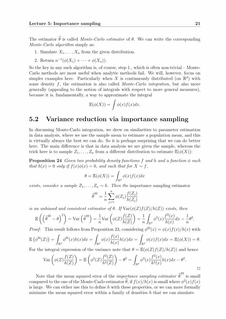
In a simulation of n = 10, 000, 000 samples for σ = 1 and c = 3, we found samplestandard deviations as in the following table, so we see that µ ≈ 3.15 gives the bestaccuracy, three significant digits estimating P(X > 3) by 0.00135, whereas only the firstdigit was significant for the Monte-Carlo estimator.

µ standard deviation estimate lower 95%CI upper 95%CI

0.00 11.5827300e-06 1.343400e-03 1.320698e-03 1.366102e-031.00 2.9066300e-06 1.352702e-03 1.347005e-03 1.358398e-032.00 1.1767060e-06 1.351572e-03 1.349266e-03 1.353878e-033.00 0.7855584e-06 1.350020e-03 1.348480e-03 1.351559e-033.10 0.7797804e-06 1.349173e-03 1.347645e-03 1.350701e-033.15 0.7791837e-06 1.349363e-03 1.347835e-03 1.350890e-033.20 0.7793362e-06 1.348548e-03 1.347020e-03 1.350075e-034.00 0.9765308e-06 1.348453e-03 1.346539e-03 1.350367e-03

Lecture 5: Importance sampling 23

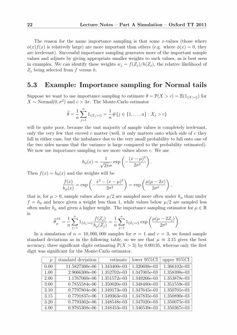
The confidence intervals are also displayed in Figure 5.1.

Figure 5.1: Confidence intervals for P(X > 3) as 0 ≤ µ ≤ 6, with µ = 3.15 emphasized.

Going a bit further for c = 4.5, Monte-Carlo does not find any significant digits;importance sampling still finds two significant digits P(X > 4.5) ≈ 0.0000034:

µ standard deviation estimate lower 95%CI upper 95%CI

0.0 556.775600e-09 3.100000e-06 2.008740e-06 4.191260e-064.5 2.423704e-09 3.397638e-06 3.392887e-06 3.402388e-064.6 2.414115e-09 3.394935e-06 3.390203e-06 3.399666e-064.7 2.419696e-09 3.393120e-06 3.388377e-06 3.397862e-06

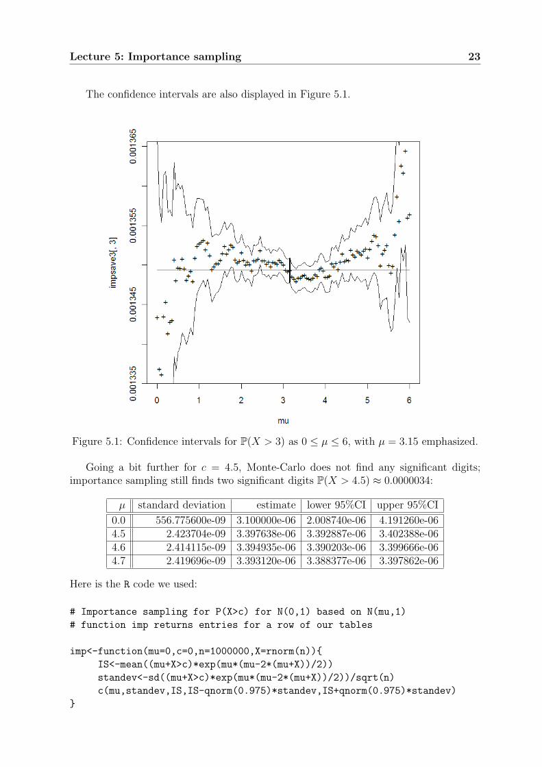
Here is the R code we used:

# Importance sampling for P(X>c) for N(0,1) based on N(mu,1)

# function imp returns entries for a row of our tables

imp<-function(mu=0,c=0,n=1000000,X=rnorm(n))

IS<-mean((mu+X>c)*exp(mu*(mu-2*(mu+X))/2))

standev<-sd((mu+X>c)*exp(mu*(mu-2*(mu+X))/2))/sqrt(n)

c(mu,standev,IS,IS-qnorm(0.975)*standev,IS+qnorm(0.975)*standev)


n<-10000000 #we fix n and X in advance

X<-rnorm(n) #and use the same random numbers for all estimates

c<-3

imp(0,c,n,X)

imp(1,c,n,X)

imp(2,c,n,X)

imp(3,c,n,X)

imp(3.1,c,n,X)

imp(3.15,c,n,X) #we find the (near-)optimal value of mu slightly above c

imp(3.2,c,n,X)

imp(4,c,n,X)

c<-4.5

imp(0,c,n,X)

imp(4.5,c,n,X)

imp(4.6,c,n,X) #we find the (near-)optimal value of mu slightly above c

imp(4.7,c,n,X)

#To plot confidence intervals as mu varies

mu<-(0:120)/20 #choose range from 0 to 6 in steps of 0.05

impsave3<-matrix(1:605,121,5) #initialize impsave3, to save imp for c=3

for (i in 1:121)impsave3[i,]<-imp(mu[i],c,n,X) #save imp in impsave3

plot(mu,impsave3[,3],pch="+") #estimates

lines(mu,impsave3[,4]) #lower CI bound

lines(mu,impsave3[,5]) #upper CI bound

lines(c(3.15,3.15),c(impsave3[64,4],impsave3[64,5])) #emphasize mu=3.15

lines(c(3.14,3.14),c(impsave3[64,4],impsave3[64,5])) #line too thin

lines(c(3.16,3.16),c(impsave3[64,4],impsave3[64,5])) #add a bit more

lines(c(0,6),c(impsave3[64,3],impsave3[64,3])) #horizontal line

Lecture 6

Markov chain Monte-Carlo

Reading: Norris Section 5.5, Ross Sections 10.1-10.2Further reading: Norris Chapter 1, Robert and Casella Sections 6.1-6.2

6.1 Simulation of Markov chains

Let X be a countable state space suitably enumerated such that we can think of a vectorλ = (λi, i ∈ X ) as a row vector of initial probabilities P(X0 = i) = λi – we suppose thatλi ≥ 0, i ∈ X and

∑i∈X λi = 1. For a transition matrix P = (pi,j, i, j ∈ X ) – non-

negative entries with unit row sums – we consider the (λ, P )-Markov chain (X0, . . . , Xn)with distribution

P(X0 = i0, . . . , Xn = in) = λi0

n∏

j=1

pij−1,ij , i0, . . . , in ∈ X .

In other words, the probability of a path i0 → i1 → · · · → in−1 → in is the probability λi0

of initial value i0 successively multiplied into all one-step transition probabilities pij−1,ij

from ij−1 to ij.Each row pi,• = (pi,j, j ∈ X ), of P , i ∈ X , is a probability distribution on X , and if

we can simulate (from the initial distribution λ and) from each of these rows pi,•, i ∈ X ,e.g. using a sequential inversion algorithm as in Section 4.3, we can simulate the chain:

1. Generate X0 ∼ λ.

2. For k from 1 to n, generate Xk ∼ pXk−1,•.

3. Return (X0, . . . , Xn).

Example 25 (Simple random walk) A particle starting from 0 (set λ0 = 1) is movingon X = Z, up with probability p ∈ (0, 1), down with probability 1 − p:

pi,i+1 = p, pi,i−1 = 1 − p, pi,j = 0 otherwise.

Figure 6.1 simulates n steps of this Markov chain. Recall that simple random walk isirreducible, but 2-periodic, and transient except when p = 1/2 in which case it is null-recurrent. In any case, there is no stationary distribution and hence no convergence tostationarity of P(Xn = k) as n → ∞. Instead, it can be shown that P(Xn = k) → 0 asn → ∞.

25


p<-0.5

n<-100

X<-rep(NA,n)

X[1]<-0

for (j in 2:n)

X[j]<-X[j-1]+2*(runif(1)<=p)-1

time<-1:n

plot(time,X,type="l")

Figure 6.1: Simple symmetric random walk

6.2 Monte-Carlo algorithm

The Monte-Carlo algorithm of Lecture 5, for the estimation of θ = E(φ(X)), was basedon independent X1, . . . , Xn with the same distribution as X, setting

θ =1

n

n∑

j=1

φ(Xj) → E(φ(X)) in probability (or a.s.) as n → ∞.

For irreducible Markov chains (X0, . . . , Xn−1) with stationary distribution π = πP , theErgodic Theorem makes a very similar statement

1

n

n−1∑

j=0

φ(Xj) → E(φ(X)) =∑

i∈X

φ(i)πi, in probability (or a.s.) as n → ∞,

where X ∼ π. If furthermore X0 ∼ π, then

P(X1 = j) =∑

i∈X

P(X1 = j|X0 = i)πi = (πP )j = πj, so X1 ∼ π,

and, inductively, X0, . . . , Xn−1 are identically distributed, but not (in general) indepen-dent. Writing pi,• for the ith row of P , the associated Monte-Carlo algorithm is:

1. Generate X0 ∼ λ.

2. For k from 1 to n − 1, generate Xk ∼ pXk−1,•.

3. Return n−1(φ(X0) + · · · + φ(Xn−1)).

Ideally, λ = π, which gives an unbiased estimator. In practice, it is often difficult tosimulate from π, so other λ are often taken – the bias disappears asymptotically.

When applying a Markov chain Monte-Carlo algorithm, the quantity of interest isusually not the Markov chain, but (some weighted sum over) stationary probabilities.Indeed, the Markov chain Monte-Carlo method is a method to approximate a distributionπ or weighted sum

∑i∈X φ(i)πi, which involves finding/choosing a suitable Markov chain.

Lecture 6: Markov chain Monte-Carlo 27

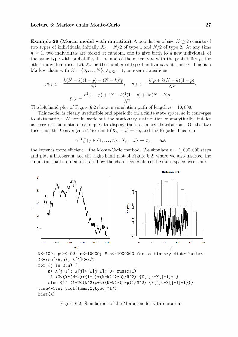
Example 26 (Moran model with mutation) A population of size N ≥ 2 consists oftwo types of individuals, initially X0 = N/2 of type 1 and N/2 of type 2. At any timen ≥ 1, two individuals are picked at random, one to give birth to a new individual, ofthe same type with probability 1 − p, and of the other type with the probability p; theother individual dies. Let Xn be the number of type-1 individuals at time n. This is aMarkov chain with X = 0, . . . , N, λN/2 = 1, non-zero transitions

pk,k+1 =k(N − k)(1 − p) + (N − k)2p

N2, pk,k−1 =

k2p + k(N − k)(1 − p)

N2,

pk,k =k2(1 − p) + (N − k)2(1 − p) + 2k(N − k)p

N2.

The left-hand plot of Figure 6.2 shows a simulation path of length n = 10, 000.This model is clearly irreducible and aperiodic on a finite state space, so it converges

to stationarity. We could work out the stationary distribution π analytically, but letus here use simulation techniques to display the stationary distribution. Of the twotheorems, the Convergence Theorem P(Xn = k) → πk and the Ergodic Theorem

n−1#j ∈ 1, . . . , n : Xj = k → πk a.s.

the latter is more efficient – the Monte-Carlo method. We simulate n = 1, 000, 000 stepsand plot a histogram, see the right-hand plot of Figure 6.2, where we also inserted thesimulation path to demonstrate how the chain has explored the state space over time.

N<-100; p<-0.02; n<-10000; # n<-1000000 for stationary distribution

X<-rep(NA,n); X[1]<-N/2

for (j in 2:n)

k<-X[j-1]; X[j]<-X[j-1]; U<-runif(1)

if (U<(k*(N-k)*(1-p)+(N-k)^2*p)/N^2) X[j]<-X[j-1]+1

else if (1-U<(k^2*p+k*(N-k)*(1-p))/N^2) X[j]<-X[j-1]-1

time<-1:n; plot(time,X,type="l")

hist(X)

Figure 6.2: Simulations of the Moran model with mutation


6.3 Reversible Markov chains

A Markov chain is called reversible if for all n ≥ 1 and i0, i1, . . . , in−1, in ∈ X , we have

P(X0 = i0, X1 = i1, . . . , Xn−1 = in−1, Xn = in) = P(X0 = in, X1 = in−1, . . . , Xn−1 = i1, Xn = i0).

In particular, this implies that for n = 1 and i, j ∈ X ,

λipi,j = P(X0 = i, X1 = j) = P(X0 = j, X1 = i) = λjpj,i.

These relations are called detailed balance equations. Summing over i, we see that

(λP )j =∑

i∈X

λipi,j =∑

i∈X

λjpj,i = λj

∑

i∈X

pj,i = λj, i.e. λ stationary.

Furthermore, if the detailed balance equations hold, the chain is already reversible:

P(X0 = i0, X1 = i1, . . . , Xn−1 = in−1, Xn = in) = λi0pi0,i1 · · · pin−1,in = pi1,i0pi2,i1 · · · pin,in−1λin

= P(X0 = in, X1 = in−1, . . . , Xn−1 = i1, Xn = i0).

Example 27 Let X = 0, . . . , N. Any transition matrix P with pi,i−1 > 0 and pi−1,i >0, i ∈ 1, . . . , n and pi,j = 0 for |i − j| ≥ 2 gives rise to a reversible Markov chain.Specifically, note that πipi,j = πjpj,i holds trivially for i = j and |i − j| ≥ 2. Theonly non-trivial detailed balance equations are πipi,i−1 = πi−1pi−1,i, i ∈ 1, . . . , n. Astraightforward induction shows that they are equivalent to

πj = π0

j∏

i=1

pi−1,i

pi,i−1

, j ∈ X ,

and the normalisation condition∑

j∈X πj = 1 yields a unique solution π. Note further,that this chain is irreducible and so π is the unique stationary distribution of this Markovchain.

Not every Markov chain that has a stationary distribution is reversible, but reversibil-ity is easy to check and useful to calculate a stationary distribution (certainly easier thansolving π = πP , usually). We will construct reversible Markov chains with a givenstationary distribution.

6.4 The Metropolis-Hastings algorithm

Let X be a finite state space and π be a distribution on X with πi > 0 for all i ∈ X . Forany initial distribution λ on X and irreducible transition matrix R = (ri,j, i, j ∈ X ) onX with ri,j = 0 ⇐⇒ rj,i = 0, consider the following Metropolis-Hastings algorithm:

1. Let X0 ∼ λ and k = 0.

2. Set k := k + 1. Generate independent Yk ∼ rXk−1,• and U ∼ Unif(0, 1).

3. If UπXk−1rXk−1,Yk

≤ πYkrYk,Xk−1

, set Xk = Yk, otherwise set Xk = Xk−1.

4. If k < n, go to 2., otherwise return (X0, . . . , Xn).

We will show that this algorithm simulates a reversible Markov chain with stationarydistribution π.

Lecture 7

The Metropolis-Hastings algorithm

Reading: Norris Section 5.5

7.1 The basic Metropolis-Hastings algorithm

Recall the basic Metropolis-Hastings setting: a finite state space X and a distributionπ on X with πi > 0 for all i ∈ X ; for any initial distribution λ on X and irreducibletransition matrix R = (ri,j, i, j ∈ X ) on X with ri,j = 0 ⇐⇒ rj,i = 0, consider:

1. Let X0 ∼ λ and k = 0.

2. Set k := k + 1. Generate independent Yk ∼ rXk−1,• and U ∼ Unif(0, 1).

3. If UπXk−1rXk−1,Yk

≤ πYkrYk,Xk−1

, set Xk = Yk, otherwise set Xk = Xk−1.


Proposition 28 Under the assumptions above, the Metropolis-Hastings algorithm sim-ulates a Markov chain with transition matrix P = (pi,j, i, j ∈ X ), where

pi,j = min

ri,j,

πjrj,i

πi

, i 6= j and pi,i = 1 −

∑

j∈X :j 6=i

pi,j.

The P -Markov chain is irreducible and reversible with stationary distribution π.

Proof: The Markov property follows directly from the explicit sequential nature of thealgorithm that only draws on Xk−1 and independent randomness from U ∼ Unif(0, 1).For the transition probabilities, note that for i 6= j

pi,j = P(Yk = j|Xk−1 = i)P

(U ≤ πYk

rYk,Xk−1

πXk−1rXk−1,Yk

∣∣∣∣Xk−1 = i, Yk = j

)= ri,j min

1,

πjrj,i

πiri,j

,

any rejection leads to a transition i → i accumulating the remaining probability mass.Irreducibility of P follows from irreducibility of R, because the hypotheses on R and

π ensure thatpi,j > 0 ⇐⇒ ri,j > 0, πj > 0, rj,i > 0 ⇐⇒ ri,j > 0.

For reversibility, note that for any i, j ∈ X , i 6= j, we have πjrj,i ≥ πiri,j or πjrj,i ≤ πiri,j.In the first case, we have pi,j = ri,j and pj,i = πiri,j/πj = πipi,j/πj. The second casefollows by symmetry. 2

29


Corollary 29 For any function φ : X → R, the Monte-Carlo estimator is consistent:

1

n

n−1∑

j=0

φ(Xj) → E(φ(X)) =∑

i∈X

φ(i)πi. in probability (a.s.) as n → ∞.

Proof: The Ergodic Theorem applies as the chain is irreducible and X finite. 2

Example 30 Consider the distribution πj = j/Zm, j ∈ X = 1, . . . ,m, where Zm =m(m+1)/2 is the normalisation constant. We use simple random walk ri,i+1 = 1−ri,i−1 =p for j ∈ 2, . . . ,m−1 with boundary transitions r1,2 = rm,m−1 = 1. Then the acceptancecondition, for j = i + 1 ∈ 3, . . . ,m − 1 can be written as

Uπi+1ri+1,i ≤ πiri,i+1 ⇐⇒ U ≤ ip

(i + 1)(1 − p).

Similarly, for j = i − 1 ∈ 2, . . . ,m − 2,

Uπi−1ri−1,i ≤ πiri,i−1 ⇐⇒ U ≤ i(1 − p)

(i − 1)(1 − p).

The boundary cases are similar. The thresholds are

2 → 1 :1

2(1−p), 1 → 2 : 2p, (m−1) → m :

m

(m−1)p, m → (m−1) :

(m−1)(1−p)

m.

The resulting Markov chain with stationary distribution π has transition probabililities

pi,j = min

ri,j,

πj

πi

rj,i

= min

ri,j,

j

irj,i

, pi,i = 1 −

∑

j∈X :j 6=i

pi,j,

which we leave in this form. Since the stationary distribution puts more weight into higherstates, we get fewer rejections and hence better mixing properties (faster convergence tostationarity) by choosing p ≥ 1/2, but not too close to 1.

Here is an example that gives rise to a Markov chain Monte-Carlo algorithm that isnot a Metropolis-Hastings algorithm, i.e. a non-example in our context here.

Example 31 Consider the Markov chain with transition matrix P = (pi,j, i, j ∈ X ),where X = 1, . . . ,m and

pi,i−1 =i − 1

i, pi,m =

1

i, i ∈ X .

It is easy to check that πi = i/Zm is the stationary distribution of this Markov chain.How did we find the chain? We exploited the special structure of the problem, withincreasing probability mass function and solved equations πP = π for P , together withpi,j = 0 except for j = m or j = i − 1. This chain is not reversible, because πipi,i−1 > 0while πi−1pi−1,i = 0 for i < m. This example of constructing a Markov chain with givenstationary distribution does not generalise to general state space. The strength of theMetropolis-Hastings algorithm is that it applies in extremely general situations. Theremay well be “better” Markov chains.

Lecture 7: The Metropolis-Hastings algorithm 31

7.2 The Metropolis-Hastings algorithm in a more

general setting

In the last section we made a number of assumption that can be relaxed.

• If X is countably infinite, the proof of Proposition 28 remains valid. The proofof Corollary 29 now relies on a different version of the Ergodic Theorem. In fact,irreducibility and the existence of a stationary distribution are enough for the con-clusion to hold, and these are both provided by Proposition 28.

• If we allow πi = 0 for some i ∈ X , the Metropolis-Hastings algorithm still simulatesa reversible Markov chain with transition matrix P . Since pi,j = 0 if πi > 0 andπj = 0, we can restrict the state space of the P -chain (but not of the R-chain) to

X = i ∈ X : πi > 0. Irreducibility is not automatic and needs to be checked caseby case. This is important, because in the reducible case, the stationary distributionis not unique and the Ergodic Theorem will apply on each communicating class,converging to different stationary distributions and not to π. If the P -chain isirreducible, the Monte-Carlo estimator is consistent.

• If we allow one-way transitions ri,j > 0 while rj,i = 0, we will have pi,j = pj,i = 0(unless πi = 0, but in that case we restrict the state space of the P -chain to

X , so these transitions are irrelevant). Again, the Metropolis-Hastings algorithmsimulates a reversible Markov chain, but irreducibility does not follow, in general. Ifwe modify the proposal transition matrix R into a matrix R by disallowing one-waytransitions in R, i.e.

ri,j =

ri,j if rj,i > 0,0 otherwise,

and ri,i = ri,i +∑

j∈X :rj,i=0

ri,j,

we find P = P for the associated Metropolis-Hastings chains. Hence, we can assumeri,j > 0 ⇐⇒ rj,i > 0 without loss of generality.

Example 32 Here are (trivial) examples to demonstrate the irreducibility problems:

(a) Consider a random walk on X = 1, 2, 3 arranged as 1 ↔ 2 ↔ 3:

R =

0 1 01/2 0 1/20 1 0

, π = (1/2, 0, 1/2).

R is irreducible, but 1 and 3 only communicate via 2, and π2 = 0 makes p1,2 =p3,2 = 0. With p1,3 = p3,1 = 0 inherited from r1,3 = r3,1 = 0, we find

P =

1 0 01/2 0 1/20 0 1

has a very different class structure: closed classes 1 and 3 and an open class2 that is irrelevant for the Monte-Carlo limits.


(b) Consider a (deterministic) walk on X = 1, 2, 3 arranged in a circle 1 → 2 → 3 → 1

R =

0 1 00 0 11 0 0

, π = (1/3, 1/3, 1/3).

R is irreducible, but all transitions are one-way; indeed

P =

1 0 00 1 00 0 1

has a different class structure: three closed classes 1, 2 and 3.

7.3 Example: the Ising model

Most of our applications and examples have been rather elementary simulations that donot bear justice to the power of simulation to penetrate beyond the bounds of analytictractability. To give a flavour of such applications (albeit still analytically tractable),consider the Ising model: on a finite integer lattice Λ = (Z/NZ)2 = 0, . . . , N − 12,equipped with the usual (horizontal and vertical, but not diagonal) neighbour relationλ ∼ µ, each lattice point λ = (i, j) ∈ Λ has one of two types s(λ) = s(i, j) ∈ 0, 1. Thespace of possible states of this system is

X = 0, 1Λ = s : Λ → 0, 1Physicists consider the following Gibbs distributions on X

π(s) =1

Zβ

exp

(−β

∑

λ,µ∈Λ:λ∼µ

(s(λ) − s(µ))2

).

Let us set up a Metropolis-Hastings algorithm to simulate from this distribution. Asproposed transition mechanism we use single spin flips (turning 1 into 0 and vice versa)chosen uniformly among the N2 lattice points of Λ. Now suppose that the proposed flipis at λ = (i, j). Then a configuration s is turned into t, where t(i, j) = 1 − s(i, j) andt(µ) = s(µ) for µ 6= λ. Hence rs,t = rt,s for all s, t ∈ X and

π(t)

π(s)= exp (2β(2 − #µ ∈ Λ : µ ∼ λ, s(µ) = s(λ))) .

Therefore, the algorithm is

1. Let X0 ∼ Unif(X ) and k = 0.

2. Set k := k + 1. Generate independent V = Unif(Λ) and U ∼ Unif(0, 1).

3. If U ≤ exp (2β(2 − #µ ∈ Λ : µ ∼ V, s(µ) = s(V ))), set Xk equal to Xk−1 withthe V -bit flipped, otherwise set Xk = Xk−1.


Figure 7.1 intends to display typical configurations under the stationary distribution forvarious choices of β ∈ R. For negative values of β different types attract, while equaltypes repel, while for positive values of β the different types repel, while equal typesattract. The result is plausible for β ∈ −1, 0, 0.5, 1, possibly β = 2, but not β = 10.


Figure 7.1: Simulations of the Ising model

N<-60

beta<--1

X<-matrix(rbinom((N+2)*(N+2),1,1/2),N+2,N+2)

connect<-function(N,A) #copy neighbours from far boundary

A[1,]<-A[N+1,];A[,1]<-A[,N+1];A[N+2,]<-A[2,];A[,N+2]<-A[,2];A

n<-100000

for (k in 1:n)

X<-connect(N,X)

V1<-floor(N*runif(1))+2;V2<-floor(N*runif(1))+2

U<-runif(1)

if (U<exp(2*beta*(2-(X[V1,V2]==X[V1-1,V2])-(X[V1,V2]==X[V1+1,V2])

-(X[V1,V2]==X[V1,V2-1])-(X[V1,V2]==X[V1,V2+1]))))

X[V1,V2]<-1-X[V1,V2]

Z1<-rep(NA,N^2);Z2<-rep(NA,N^2)

k<-1

for (i in 1:N)

for (j in 1:N)

if (X[i+1,j+1]==1)

Z1[k]<-i-1;Z2[k]<-j-1;k<-k+1

plot(Z1,Z2,pch=16,main=paste("Ising model with N=",N," and beta=",beta))


For β = 0, all proposed swaps are accepted. For β → ∞, there are two best con-figurations, namely “all type 0” and “all type 1” that, asymptotically, take probability1/2 each under the stationary distribution – there are only finitely many configurationsand the next likely configurations are the ones with only one site of different type, butthese are already separated by a multiplicative factor of exp(−4β) → 0. This factor isalready quite small and means that it is extremely unlikely to create new islands of onetype within another, and if so they disappear again quickly. However, the algorithm firstcreates regions of both types that compete, with lots of activity back and forth at theirboundary. It takes a long time for the last regions of the losing type to get smaller anddisappear.

N<-60

beta<-10


Z1<-rep(NA,N^2);Z2<-rep(NA,N^2)

k<-1

for (i in 1:N)

for (j in 1:N)

if (X[i+1,j+1]==1)

Z1[k]<-i-1;Z2[k]<-j-1;k<-k+1

plot(Z1,Z2,pch=16,main=paste("Ising model with N=",N," and beta=",beta))

connect<-function(N,A) #copy neighbours from far boundary

A[1,]<-A[N+1,];A[,1]<-A[,N+1];A[N+2,]<-A[2,];A[,N+2]<-A[,2];A

n<-100000

for (k in 1:n)

X<-connect(N,X)

V1<-floor(N*runif(1))+2;V2<-floor(N*runif(1))+2

U<-runif(1)

if (U<exp(2*beta*(2-(X[V1,V2]==X[V1-1,V2])-(X[V1,V2]==X[V1+1,V2])

-(X[V1,V2]==X[V1,V2-1])-(X[V1,V2]==X[V1,V2+1]))))

X[V1,V2]<-1-X[V1,V2]

if (X[V1,V2]==1) points(V1-2,V2-2,col="black",pch=16)

else points(V1-2,V2-2,col="white",pch=16)

else points(V1-2,V2-2,col=k) #coloured open circles display rejections

This was all on a torus (i.e. with 0 neighbouring N − 1 in both directions). Instead ofconnecting this way, we can fix boundary conditions, say all type 0, or type 0 on the lefthalf and type 1 on the right. This influences the behaviour. In the code, just remove theconnect line and set up the initial matrix as


X[1,]<-0;X[N+2,]<-1;X[,1]<-0;X[,N+2]<-1


For the case of fixed boundary, Figure 7.2 shows three simulations with uniformrandom initial conditions (top) and three simulations (bottom) from the initial conditionthat is most likely under the stationary distribution, which has an upper triangle oftype 1 and a lower triangle of type 0, so we see the fluctuations away from the optimalconfiguration, all for β = 10 here. This demonstrates, in particular, that convergenceto stationarity has not happened in the simulations that started from uniform randominitial conditions.

Figure 7.2: Simulations of the Ising model for β = 10 with fixed boundary

Here is the code for the upper triangular initial conditions:

for (i in 1:N+2)

for (j in 1:N+2)

if (i+j>N+2) X[i,j]<-1

else X[i,j]<-0

Lecture 8

Unknown normalisation constants

Reading: Casella and Berger Section 3.3

8.1 Normalisation constants

All common probability distributions are based on a convergent integral or series, becausewe require probability density functions f : Rd → [0,∞) to integrate to 1 and probabilitymass functions (pj)j∈X to sum up to 1. This nearly always means that they are naturallywritten in the form

f(x) =f(x)

C, where C =

∫

Rd

f(x)dx, or pj =pj

C, where C =

∑

j∈X

pj,

where f or p is “simpler”.

Example 33 (i) Uniform distribution f(x) = 1, x ∈ D, for some D ⊂ Rd of finitevolume Vol(D); here C = Vol(D).

(ii) Uniform distribution pj = 1, j ∈ X , for some finite set X ; here C = #X .

(iii) Poisson distribution pj = λj/j!, j ≥ 0, for some λ ∈ (0,∞); here C = eλ, by theexponential series.

(iv) Gamma distribution f(x) = xα−1e−λx, x > 0, for some α, λ ∈ (0,∞); here C =Γ(α)/λα, by the Gamma integral (and a linear change of variables y = λx).

(v) Beta distribution f(x) = xα−1(1−x)β−1; here C = Γ(α)Γ(β)/Γ(α+β), by the Betaintegral.

(vi) Normal distribution f(x) = exp(−(x − µ)2/2σ2), for some µ ∈ R, σ2 > 0; hereC =

√2πσ2.

(vii) Gibbs distribution pj = exp(−H(j)) = exp(−∑

i∈Λ h(ji)), j = (ji, i ∈ Λ) ∈ X =SΛ for some finite sets S and Λ and some function h : S → R.

37


8.2 Rejection method

As mentioned before, normalisation constants of proposal and target distribution alwayscancel in the rejection method, because the (optimal) acceptance condition is

supf(x)/h(x) : x ∈ RdUh(X) ≤ f(X) ⇐⇒ supf(x)/h(x) : x ∈ RdUh(X) ≤ f(X),

or, respectively in the discrete setting

supπ(j)/ξ(j) : j ∈ XUξ(X) ≤ π(X) ⇐⇒ supπ(j)/ξ(j) : j ∈ XUξ(X) ≤ π(X).

We can actually go one step further and use the rejection algorithm to estimate normal-isation constants. Specifically, recall that the number of trials up to and including thefirst acceptance is geom(1/M), where (in the continuous case, say)

M = supf(x)/h(x) : x ∈ Rd = supf(x)Ceh/h(x)C ef : x ∈ Rd

=Ceh

C ef

supf(x)/h(x) : x ∈ Rd.

The maximum likelihood estimator for geom(p) based on a sample N1, . . . , Nn is

p =n

N1 + · · · + Nn

,

and we need M = supf(x)/h(x) : x ∈ Rd to implement the algorithm, so we can use

Ceh/C ef =1

Mp=

1

Mn

n∑

i=1

Ni.

This estimator is unbiased as E(Ni) = 1/M , and it is independent from the acceptedsample. If the proposal constant Ceh is known, we obtain an unbiased estimator for the(reciprocal of the) target constant 1/C ef :

1/C ef =1

MCehn

n∑

i=1

Ni.

8.3 Importance sampling

In order to implement importance sampling as in Lecture 5 we have to know normalisationconstants, since

θIS

=1

n

n∑

j=1

φ(Zj)f(Zj)

h(Zj),

cf. Proposition 24. There is an Importance Sampling estimator for un-normalized densi-ties too, and it is in this form that Importance Sampling estimation is usually conducted.

Let f , h : Rd → [0,∞) be unnormalised probability density functions and φ : Rd → R

a function. Denote by C ef =∫

Rd f(x)dx and Ceh =∫

Rd h(x)dx the normalisation constants

that lead to probability density functions f = f/C ef and h = h/Ceh. Suppose that wewish to estimate θ = E(φ(X)) = E(φ(Z)f(Z)/h(Z)) for a random variable X ∼ f usingimportance sampling based on a sample Z1, . . . , Zn ∼ h.

Lecture 8: Unknown normalisation constants 39

If the normalizing constants C ef and Ceh are not available, we separate them out and write

E

(φ(Z)

f(Z)

h(Z)

)=

Ceh

C ef

E

(φ(Z)

f(Z)

h(Z)

).

Note that (taking φ ≡ 1), we have an unbiased estimator for C ef/Ceh:

E

(f(Z)

h(Z)

)=

C ef

Ceh

E

(φ(Z)

f(Z)

h(Z)

)=

C ef

Ceh

E(φ(X)) =C ef

Ceh

.

It follows that (for general φ : Rd → R)

E(φ(X)) =E(φ(Z)f(Z)/h(Z)

E(f(Z)/h(Z)),

and we can estimate the numerator (A, say) and denominator (B, say) separately.The resulting algorithm for the estimation of E(φ(X)) is:

1. Simulate independent Z1, . . . , Zn ∼ h.

2. Set w(Zj) = f(Zj)/h(Zj), for all j = 1, . . . , n.

3. Set A =1

n

n∑

j=1

w(Zj)φ(Zj) and B =1

n

n∑

j=1

w(Zj).

4. Return the ratio θIS

R = A/B as modified Importance Sampling estimate for E(φ(X)).

While E(A) = E(φ(Z)f(Z)/h(Z)) = A and E(B) = B, we have E( θIS

R ) 6= θ = E(φ(X)),in general, since the expectation of a ratio is not (usually) the ratio of expectations. In ouralgorithm we use the same sample Z1, . . . , Zn to estimate numerator and denominator,but even if we used independent samples, we would still end up with E(1/B) 6= 1/E(B) =1/B. In fact, this latter inequality is always “strictly greater than” (by a form of Jensen’s

Inequality). In other words, while A and B are unbiased, θIS

R may be biased.

Proposition 34 The modified Importance Sampling estimator θIS

R is consistent:

θIS

R → θ (in probability or a.s.) as n → ∞.

Proof: As in Proposition 23, (weak or strong) consistency of A, and also of B, follows

from the (Weak or Strong) Law of Large Numbers, applied to Yj = φ(Zj)f(Zj)/h(Zj),

with φ ≡ 1 in the case of B. Strong consistency means

P(A → A) = 1

P(B → B) = 1⇒ P(A → A and B → B) = 1 ⇒ P

(A

B→ A

B

)= 1.

But since almost sure convergence and the Strong Law of Large Numbers are not Part

A material, we give a rather more cumbersome direct proof of weak consistency of θIS

R ,which establishes the ratio part of the algebra of limits for convergence in probability.


Let us write An and Bn for A and B based on sample size n. Let ε > 0 and δ > 0. Thenwe can find n0 ≥ 0 such that for all n ≥ n0

P

(∣∣∣Bn−B∣∣∣> B

2

)<

δ

3and P

(∣∣∣An−A∣∣∣> εB

4

)<

δ

3and P

(A∣∣∣Bn−B

∣∣∣> εB2

4

)<

δ

3.

Then, we will also have for all n ≥ n0

P

(∣∣∣∣∣An

Bn

− A

B

∣∣∣∣∣>ε

)≤ P

(∣∣∣Bn−B∣∣∣> B

2

)+ P

(∣∣∣Bn−B∣∣∣≤ B

2,∣∣∣AnB−ABn

∣∣∣>εBnB

)

<δ

3+ P

(∣∣∣AnB − AB∣∣∣ > εB2

4

)+ P

(∣∣∣AB − ABn

∣∣∣ > εB2

4

)< δ,

where the middle step uses Bn > B/2, and |D1 +D2| > c ⇒ |D1| > c/2 or|D2| > c/2. 2

Example 35 We wish to estimate E(φ(X)) for the target distribution X ∼ Gamma(α, β)using the proposal distribution X ∼ Gamma(a, b), e.g. a ∈ N, i.e. where

f(x) = xα−1e−βx, h(x) = xa−1e−bx, x > 0, and C ef = β−αΓ(α), Ceh = b−aΓ(a).

Suppose we do not know C ef and Ceh (or we are not confident we can calculate it correctly

or we cannot be bothered calculating it!). Now f(x)/h(x) = xα−a exp(−(β − b)x), so:

1. Simulate independent Z1, . . . , Zn ∼ Gamma(a, b).

2. Set wj = Zα−aj exp(−(β − b)Zj), for all j = 1, . . . , n.

3. Return the modified Importance Sampling estimate θIS

R =

∑j wjφ(Zj)∑

j wj

.

Simulation studies show that often the ratio estimator θIS

R gives more stable estimates of

E(φ(X)) than the basic Importance Sampling estimator θIS

. Some authors recommend

using θIS

R even when you know and can easily calculate all the normalizing constants.This is surprising as we have an extra quantity to estimate for the ratio estimator.

8.4 Metropolis-Hastings algorithm

For π = π/C, we can also estimate C in the Metropolis-Hastings algorithm , e.g. C = #Xwith π ≡ 1, : naively, take any i ∈ X and note πi = #j ∈ 0, . . . , n− 1 : Xj = i/n →πi/C, so 1/C ≈ πi/πi. However, more sophisticated techniques are needed for big X .

8.5 Conclusion

In this lecture course, we have studied the main simulation techniques of inversion, trans-formation, rejection, importance sampling, and Markov chain Monte-Carlo methods suchas the Metropolis-Hastings algorithm. For illustration of the techniques we have mostlyused the common families of discrete and continuous probability distributions. It mustbe stressed, however, that the techniques apply much more widely, and that is wheretheir full power can be exploited – however, the introduction to application areas woulduse a disproportionate amount of time in an 8-hour lecture course, so we have largelystayed clear of such developments and refer to the literature for further reading.

Appendix A

Assignments

Assignment sheets are issued on Mondays of weeks 2-4. They are made available on thewebsite of the course at

http://www.stats.ox.ac.uk/∼winkel/ASim.html.

Two sets of three one-hour classes take place in room 102 of 1 South Parks Road (LectureRoom, Department of Statistics) in weeks 2 to 4, on Fridays, as follows:

• Fridays 11.00am-12.00pm

• Fridays 12.00-1.00pm

The class allocation can be accessed from the course website shortly after the first lecture,as soon as I have entered the details, soon after the first lecture.

Scripts are to be handed in at the Department of Statistics, 1 South Parks Road.Exercises on the problem sheets vary in style and difficulty. If you find an exercise

difficult, please do not deduce that you cannot solve the following exercises, but aim atgiving each exercise a serious try. Solutions will be provided on the course website.

There are lecture notes available. Please print these so that we can make bestuse of the lecture time. Please let me know of any typos or other comments that youmay have, e.g. by sending an email to [email protected].

I

II Assignments – Part A Simulation – Oxford TT 2011

Below are some comments on the recommended Reading and Further Reading liter-ature.

Ross: Simulation 2006

This is our main reference. The style is somewhat more elementary than our course, butour syllabus is well-coverered. There are lots of examples and exercises, so this bookis the ideal place to find more detailed explanations and illustrations, where our coursetakes bigger steps or focusses on the overall picture. We use material from most of the 11chapters, so it is best used as a reference book in conjunction with rather than insteadof these lecture notes.

Ripley: Stochastic Simulation 1987

This book is now almost 25 years and some of the detailed discussions of (old) randomnumber generators and efficiency considerations tend to play a much less prominent partnowadays. However, the issues are still there in principle, and it is still instructive tostudy them. We occasionally refer to this book. The style is concise. Some topics receivea briefer treatment than in our course, but there is much more in the book.

Robert and Casella: Monte Carlo Statistical Methods 1999

This book is more advanced than our course. Many of our topics are treated in much moredepth, so the main ideas for our course are well-spread over the book. I recommend thisbook for further developments and techniques that are specific to certain applications.

Norris: Markov Chains 1997

This is a book on the theory and applications of Markov chains, written mainly formathematicians with an interest in probability theory, but not necessarily statistics.Only Section 5.5 discusses a simulation topic: Markov chain Monte Carlo. However,Norris is our main reference for that part of the course, i.e. for Lectures 6 and 7.

Assignment 1 – Part A Simulation – Oxford TT 2011 III

A.1 Inversion, transformation and rejection

Please hand in scripts by Wednesday 11 May 2011, 10am, Department of Statistics.2.(c) and 4. require material from Lecture 3, the others are on week 1 material only.

1. (a) Consider a random variable X with continuous and strictly increasing cumu-lative distribution function FX : R → (0, 1). Show that

FX(X) ∼ Unif(0, 1)

and thatF−1

X (U) ∼ X, where U ∼ Unif(0, 1).

(b) Consider a random variable X with any (right-continuous and non-decreasing)cumulative distribution function FX : R → [0, 1]. Let Au =z ∈ R : FX(z) > ufor all u ∈ (0, 1). Show that

u < FX(x) ⇒ inf Au ≤ x ⇒ u ≤ FX(x) for all x ∈ R and u ∈ (0, 1).

Hence, or otherwise, show that

inf AU ∼ X, where U ∼ Unif(0, 1).

Define the generalised inverse F−1X (u) = inf Au = infz ∈ R : FX(z) > u and

compare with (a); also find a necessary and sufficient condition for

FX(X) ∼ Unif(0, 1).

2. (a) Let Y ∼ Exp(λ). Fix a > 0 and consider a random variable X with

FX(x) = P(X ≤ x) = P(Y ≤ x|Y > a), x ∈ R.

For u ∈ (0, 1), calculate F−1X (u) and hence give an algorithm simulating X

based on U ∼ Unif(0, 1).

(b) Let Z be any real-valued random variable. Fix a < b with P(a < Z ≤ b) > 0and consider a random variable W with

P(W ≤ w) = P(Z ≤ w|a < Z ≤ b), w ∈ R.

Show that

F−1Z (FZ(a)(1 − U) + FZ(b)U) ∼ W, where U ∼ Unif(0, 1).

Apply this formula to simulate the random variable X from (a) above.

(c) Here is another algorithm to simulate the random variable X from (a) above:

1. Simulate Y ∼ Exp(λ);

2. if Y > a, then stop and return X = Y , otherwise go to 1.

Show that this is a rejection algorithm and identify the proposal and targetprobability density functions. Calculate the expected number of trials beforeX is simulated. Why is inversion as in (a) to be preferred for a >> 1/λ?

IV Assignments – Part A Simulation – Oxford TT 2011

3. Consider the family of distributions with probability density function

fµ,λ(x) = λ exp(−2λ|x − µ|), x ∈ R,

where λ > 0 and µ ∈ R are parameters.

(a) Given U ∼ Unif(0, 1), use the inversion method to simulate from fµ,λ.

(b) Let X have probability density function fµ,λ. Show that a+bX has probabilitydensity function fµ′,λ′ . Find the parameters µ′ and λ′.

(c) Let Y, Z ∼ Exp(r) independent. Show that Y −Z has probability density func-tion fµ′,λ′ . Find µ′ and λ′. Hence, use the transformation method to simulatefrom fµ,λ for any µ ∈ R and λ > 0, given U1, U2 ∼ Unif(0, 1) independent.

(d) Let Y, Z ∼ Exp(r) independent. Find the joint probability density function ofY − Z and Y + Z. Are Y − Z and Y + Z independent?

(e) Let Y ∼ Exp(r) and B ∼ Bernoulli(1/2). Show that a + (2B − 1)Y hasprobability density function fµ′,λ′ . Find µ′ and λ′. Hence, use the trans-formation method to simulate from fµ,λ for any µ ∈ R and λ > 0, givenU1, U2 ∼ Unif(0, 1) independent.

(f) (Optional R exercise) Implement the algorithms of (a), (c) and (e) and demon-strate statistically that they simulate from the same distribution.

4. Consider the standard normal density f(x) = (2π)−1/2 exp(−x2/2) and h(x) =12exp(−|x|), x ∈ R.

(a) Find M to bound f(x)/h(x) for all x ∈ R.

(b) Give a rejection algorithm simulating X ∼ f based on Yj ∼ h, j ≥ 1.

(c) Could we reverse things and simulate Y ∼ h by rejection based on Xj ∼ f ,j ≥ 1?

(d) (Optional R exercise) Implement your rejection algorithm for X in R.

Course website: http://www.stats.ox.ac.uk/∼winkel/ASim.html

Assignment 2 – Part A Simulation – Oxford TT 2011 V

A.2 Rejection and importance sampling

Please hand in scripts by Wednesday 18 May 2011, 10am, Department of Statistics.

1. Consider a discrete distribution on X = 1, 2, . . . ,m with probability mass func-tion π(i), i ∈ X . Let ξ(i) = 1/m be the probability mass function of the uniformdistribution on X . Give a rejection algorithm using ξ as proposal distribution and πas target distribution. Calculate the expected number of trials from ξ per returnedvalue from π if m = 4 and (π(i), 1 ≤ i ≤ 4) = (0.5, 0.25, 0.125, 0.125).

2. The negative binomial distribution NegBin(m, p) is the distribution of the numberof failures in a sequence of independent Bernoulli(p) trials run until the mth success.

(a) Show that for X ∼ NegBin(m, p),

P(X = n) =

(m + n − 1

n

)(1 − p)npm, n ≥ 0.

(b) Find a sequential inversion algorithm for the negative binomial distribution.

(c) Show that there is no rejection algorithm for the negative binomial distributionthat uses the Poisson distribution as proposal distribution.

(d) Show that the negative binomial distribution is an overdispersed Poisson dis-tribution of the form

P(X = n|R = r) =rn

n!e−r where R ∼ Gamma

(m,

p

1 − p

).

(e) Use (d) to set up a simulation algorithm for the negative binomial distributionbased on m+1 independent uniform random variables U0, . . . , Um ∼ Unif(0, 1).

(f) Which of the two algorithms in (b) and (e) is to be preferred? Can you thinkof a situation where you might prefer the other algorithm?

3. Consider the following algorithm

1. Generate independent U1 ∼ Unif(0, 1) and U2 ∼ Unif(0, 1).

2. Set (V1, V2) = (2U1 − 1, 2U2 − 1) and S = V 21 + V 2

2 .

3. If S ≤ 1, go to 4., else go to 1.

4. Set P =√−2(ln(S))/S.

5. Return the pair (X, Y ) = (PV1, PV2).

This algorithm is called the “polar method”.

(a) Show that when the algorithm goes to 4., V = (V1, V2) ∼ Unif(D), whereD = (x, y) ∈ R2 : x2 + y2 < 1 is the disk of radius 1.

(b) Show that (X, Y ) is a pair of independent standard normal random variables.

(c) Compare this algorithm with the Box-Muller algorithm. How many Unif(0, 1)variables are needed per Normal(0, 1) variable, and what functions need to beevaluated?

VI Assignments – Part A Simulation – Oxford TT 2011

4. Suppose X ∼ Normal(0, σ2) and we want to estimate µg = E(g(X)) for somefunction g known to have finite mean E(g(X)) and variance Var(g(X)). Supposewe have a random sample Y1, . . . , Yn ∼ Normal(0, 1). Here are two estimators forµg given in terms of Y1, . . . , Yn:

µ(1)g =

1

n

n∑

i=1

g(σYi)

and

µ(2)g =

1

nσ

n∑

i=1

e−Y 2

i (1/2σ2−1/2)g(Yi).

(a) Show that µ(1)g and µ

(2)g are unbiased, and calculate their variances.

(b) Show that µ(1)g is a Monte-Carlo estimator of E(g(X)), and that µ

(2)g is an

importance sampling estimator of E(g(X)) – identify associated densities fand h.

(c) For what range of values of σ has µ(2)g finite variance for all g as above? Can

you give a weaker condition if it is known that∫∞

−∞g2(x)dx < ∞?

(d) Why might we prefer µ(2)g to µ

(1)g , for some values of σ2 and functions g? [Hint:

consider estimating P(X > 1) with σ ≪ 1.]


Assignment 3 – Part A Simulation – Oxford TT 2011 VII

A.3 Importance sampling and MCMC

Please hand in scripts by Wednesday 25 May 2011, 10am, Department of Statistics.

1. Consider a random variable X with probability density function f0 : R → [0,∞).We are seeking to estimate E(φ(X)) =

∫R

φ(x)f0(x)dx for a function φ : R → R

with E(|φ(X)|) < ∞.

(a) Use the Monte-Carlo method to estimate E(φ(X)).

(b) Suppose that X has a moment generating function G : (−a, b) → (0,∞),G(t) = E(etX). Show that there is a family of probability distributions withprobability density function x 7→ fr(x) proportional to x 7→ erxf0(x). Formu-late associated importance sampling estimators of E(φ(X)).

(c) Suppose that X > 0 has moments M : (−c, d) → (0,∞), M(t) = E(X t). Usethe moments to find more importance sampling estimators of E(φ(X)).

(d) Let f0(x) = (Γ(α))−1λαxα−1 exp(−λx) be the Gamma(α, λ) density. Apply(b) and (c) to find importance sampling estimators for E(φ(X)). In each case,identify the proposal distribution that needs simulating.

(e) (Optional R exercise) Implement the algorithms in those cases where you cansimulate the proposal distribution and where either φ = 1(h,∞) or φ = 1(0,h).

2. A contingency table M is an k × ℓ matrix with integer entries mi,j ≥ 0, 1 ≤ i ≤ k,1 ≤ j ≤ ℓ, and fixed row sums r1, . . . , rk and fixed column sums c1, . . . , cℓ. Denoteby X = Xr,c the set of all such tables for given vectors r = (r1, . . . , rk) and c =(c1, . . . , cℓ).

An index table H has zero row and column sums and entries hi,j ∈ −1, 0, 1.Denote by I = Ik,ℓ the set of all k × ℓ index tables. In the sequel, you may assumethat you can simulate U ∼ Unif(I).

Given X0 ∈ X , consider the following algorithm to modify contingency tables:

1. Simulate U1 ∼ Unif(I).

2. Set X1 = X0 + U1.

Here are examples of contingency tables and index tables as in the algorithm:

M =

7 2 05 6 11 6 30 1 2

∈ X , I =

0 0 00 1 −10 −1 10 0 0

∈ I, M ′=M + I =

7 2 05 7 01 5 40 1 2

∈ X .

(a) Is +: X × I → X well-defined?

(b) Modify the algorithm by rejecting disallowed transitions (i.e. staying at thesame state instead) and repeatedly apply it to simulate a Markov chain (Xn)n≥0

in X starting from X0 = M ∈ X . Specify its transition probabilities pM,M ′ ,M, M ′ ∈ X .

(c) Show that the Markov chain in (b) is reversible with stationary distributionUnif(X ).

VIII Assignments – Part A Simulation – Oxford TT 2011

(d) Assuming without proof that for any two M, M ′ ∈ X there are I1, . . . , In ∈ Iwith M + I1 + · · ·+ In = M ′, use standard results to show that for all M ∈ X

P(Xn = M) → 1/#X , as n → ∞,

andn−1#m ∈ 0, . . . , n − 1 : Xm = M → 1/#X ,

in probability (or a.s.) as n → ∞.

(e) Explain why the algorithm in (b) can be thought of as a Metropolis-Hastingsalgorithm with proposal transitions given by the original algorithm above.

3. (a) Give a Metropolis-Hastings algorithm to sample according to the binomialprobability mass function

pk =n!

k!(n − k)!pk(1 − p)n−k, k ∈ 0, 1, . . . , n,

with parameters n ∈ N and p ∈ (0, 1). Use Unif(0, 1, . . . , n) as proposaldistribution, independent of the previous states.

(b) Give a Metropolis-Hastings algorithm to sample according to the geometricprobability mass function

pk = p(1 − p)k−1, k ∈ 1, 2, . . .,

with parameter p ∈ (0, 1). Use simple symmetric random walk as the proposaltransition matrix.

(c) (Optional R exercise) Implement the algorithms of (a) and (b) and check thatthey work by comparing estimated means and variances with the known the-oretical means and variances of theses distributions.


part a simulation - oxford statisticswinkel/asim11.pdfpart a simulation matthias winkel department...

Documents