partial coordination may increase overall costs in supply...

Decision Making in Manufacturing and ServicesVol. 2 • 2008 • No. 1–2 • pp. 47–62

Partial Coordination May Increase Overall Costsin Supply Chains

Waldemar Kaczmarczyk∗

Abstract. This paper presents a computational study to evaluate the impact of coordinatingproduction and distribution planning in a two-level industrial supply chain. Three planningmethods are compared. The first emulates the traditional way of planning. The two othercoordinate plans of the supplier and of all the buyers according to the Vendor ManagedInventory (VMI) approach. The monolithic method solves a single model describing theentire optimization problem. The sequential method copies the imperfect VMI practice.All three methods are implemented by means of Mixed Integer Programming models. Theresults presented prove that the right choice of planning method is very important for overallcost of the supply chain. In contrast to the previous research, it turned out that informationsharing without full coordination may even lead to increase in the overall cost. For somecompanies applying the VMI approach, developing exact models and solving them almostoptimally may therefore be very important.

Keywords: supply chain, production, distribution, lot-sizing, coordination, mixed integerprogrammingMathematics Subject Classification: 90B30, 90B06, 90C11

Revised: 7 November 2008

1. INTRODUCTION

In the traditional supply chain, the buyer plans his replenishment accordingly tothe end-user demand, has to bear delivery and inventory holding costs, but ignoressupplier capacity, set-up and inventory holding costs. The supplier has no informationabout the end-user demand and plans his production according to buyer orders. Thereis little place for coordination in this approach.

New cooperation relationships between buyers and suppliers that allow bettercoordination have gained in popularity over recent years. They share some commoncharacteristics (Lee and Chu, 2005):1. The buyer shares end-user demand information with the supplier,2. The supplier has full inventory control in the supply chain, keeps the inventory

and bears the risk of demand uncertainty.∗ Department of Operations Research and Information Technology, AGH University of Science and

Technology, Krakow, Poland, E-mail: [email protected]

47

48 W. Kaczmarczyk

One of them is called Vendor Managed Inventory (VMI). Under the VMI approach,downstream companies, buyers, share end-user demand information with the up-stream companies, suppliers, who should then make stock level decisions for both theupstream and the downstream. To discourage suppliers from moving to the buyersas much inventory as is allowed, VMI contracts sometimes permit buyers to returnexcess goods to the supplier or make supplier responsible for inventory holding costsat buyers’ site. VMI is also sometimes referred to as the Continuous ReplenishmentProgram (CRP) or the Continuous Product Replenishment program (CPR) in thepackaged-goods industry (Lee and Chu, 2005).

Under the terms of a VMI contract, the supplier has the opportunity to coordi-nate his production with distribution. Unfortunately, both of these planning prob-lems belong to a family of complex lot-sizing problems. The integrated productionand distribution problem may not be easier. There are several surveys on coordina-tion of production and distribution in supply chains, e.g. Thomas and Griffn (1996),Sarmiento and Nagi (1999), Erengüç et al. (1999).

There are also some computational studies evaluating impact of coordination.Sahin and Robinson Jr. (2005) evaluated different strategies in the make-to-orderenvironment: four with none or partial information sharing, with none or partialcoordination, and one with full information sharing and full coordination. For vari-ous data parameters, i.e. the number of items, supplier equipment changeover cost,delivery fixed cost or demand variability, they reported an average of 47.58% systemwide cost reduction when moving from a traditional strategy to a fully coordinatedsupply chain. In their opinion, tighter coordination among channel members mayprovide a more effective lever for cost improvement than information sharing.

Chandra and Fisher (1994) report from 3% to 20% reduction in the total operatingcost with coordination for various data sets. Furthermore, they concluded that thevalue of coordination increases when the supplier production capacity decreases on theone hand, or the length of the planning horizon, the number of products or customersincrease on the other hand.

In this paper, three planning methods are compared. The first emulates the tradi-tional way of planning, where all the buyers make their replenishment decisions andthe supplier plans his production to satisfy buyers’ demand. The two other coordi-nate plans of the supplier and of all the buyers according to the Vendor ManagedInventory (VMI) approach. The monolithic method solves a single model describingthe entire optimization problem. The sequential method copies the imperfect VMIpractice, and first schedules the suppliers’ production for the aggregated demand ofall the buyers and then solves the distribution problem. Both methods assume thata single decision maker has full information and all decisions in his hand, different isonly the way he/she makes use of it. The monolithic method tries to solve one bigmodel, which is difficult due to its complexity. The sequential method decomposesthe problem into two subproblems, similarly to the traditional method, but solvesthem in a different order, more natural for the supplier.

The traditional method does not coordinate production and distribution in anyway. The monolithic method strives for full coordination. The sequential method ap-plies partial coordination, i.e. plans production simultaneously for all the buyers but

Partial Coordination May Increase Overall Costs in Supply Chains 49

ignores dependence of the production schedule on distribution costs and constraints.The objective of this study is to investigate the impact of these planning methods onthe overall supply chain cost at various parameters settings.

The model examined in this paper was inspired by Miodońska (2006) who dis-cussed distribution planning in the automotive industry. Automobile manufacturers,buyers of car components, usually work in the just-in-time fashion, i.e. do not doany batching. This leads to rather stationary product mix and stationary demandfor components. Therefore, component suppliers cooperating with car manufacturersin the VMI fashion do not have to face lumpy demand. On the other hand, mostsuppliers have to deal with relatively high set-up costs and fixed delivery costs, whichforces batching of production and deliveries.

In the next section, the monolithic Mixed Integer Programming (MIP) model ofthe problem at hand is presented. Section 3 describes decomposition procedures, thetraditional and sequential methods. Section 4 presents data parameters and section 5provides results of experiments. Conclusions are made in section 6.

2. MONOLITHIC METHOD

In the problem at hand, several components are produced over time by a single sup-plier. Setup costs are reasonable with one set-up a day at the most. Joint deliveriesof all components to several buyers are done with tracks of various capacity, fixed costand delivery time. The daily demand for each component of each buyer is known.The problem is to schedule production and distribution so as to minimize the totalcost of the inventory, production and transportation set-ups. Table 1 defines all theparameters and Table 2 provides all the variables in the model.

Table 1. Data parameters

T = {1, . . . , T} - a set of periods (days), where T stands for the number of periods,N = a set of components,K – a set of buyers,L – a set of trucks,djkt – demand of buyer k for component j in period t,hjk – holding cost of component j at buyer k, where k = 0 represents the supplier,pj – unit processing time of component j,Ct – production capacity in period t,sj – start-up cost of component j,Ll – capacity of truck l,qkl – (also q(k, l)) transport time to buyer k with truck l,cl – delivery (transportation) fixed cost with truck l,ejk – unit cost of lost demand for component j at buyer k.

50 W. Kaczmarczyk

Safety stocks required by buyers and initial inventories can be subtracted fromdemand of initial periods and therefore do not have to be taken into consideration.All components have the same size and weight.

Table 2. Variables

xjt – production volume of component j in period t,yjt = 1, if component j is set-up in period t, 0 else,zjt = 1, if component j is start-up in period t, 0 else,ujklt – volume of delivery of component j sent to buyer k in period t, i.e. it will be

available for buyers in period t + qkl,wklt = 1, if in period t truck s is sent to buyer k, 0 else,Ijkt – inventory of component j at the end of period t at buyer k, where t = 0

stands for the initial inventory and k = 0 for the inventory of the supplier,fjkt – lost demand of component j at buyer k in period t.

The set-up variables yjt describe the state of the machines, i.e. which componentscan be produced on a given day. The start-up variables zjt describe changes in thestate of the machines, i.e. if yj,t−1 = 0 and yjt = 1 then zjt = 1, otherwise zjt = 0.

The following monolithic model (1) describes all the cost factors and all the con-straints of the integrated production-distribution problem.

min∑j∈N

∑t∈T

(sjzjt + hj0Ij0t +

∑k∈K

(hjkIjkt + ejkfjkt

))+∑k∈K

∑l∈L

∑t∈T

(clwklt +

∑j∈N

qklhjkujklt

)(1a)

s.t. Ijk,t−1 +∑l∈L

ujkl,t−q(k,l) − djkt + fjkt = Ijkt, t ∈ T , j ∈ N , k ∈ K, (1b)∑j∈N

ujklt ≤ Lswklt, t ∈ T , k ∈ K, l ∈ L, (1c)

Ij0,t−1 + xjt −∑k∈K

∑l∈L

ujklt = Ij0t, t ∈ T , j ∈ N , (1d)

xjt ≤ Bjtyjt, t ∈ T , j ∈ N , (1e)∑j∈N

yjt ≤ 1, t ∈ T , (1f)

yjt − yj,t−1 ≤ zjt, t ∈ T , j ∈ N , (1g)xjt, ujklt, Ijkt ≥ 0, t ∈ T , j ∈ N , (1h)

k ∈ K, l ∈ L,

yjt, zjt, wklt ∈ {0, 1}, t ∈ T , j ∈ N , (1i)k ∈ K, l ∈ L.


Bjt = min{Ct/pjt,∑

l=t,...,T djl} is a number not smaller than xjt. The objectivefunction (1a) summarizes all the costs: the costs of the supplier, then of all thebuyers, and finally the costs of distribution. Included are the costs of the “inventoryon wheels”, i.e. during transport, to prevent any unreasonable preference for slowercars. Constraint (1b) preserves balance of deliveries, inventory and end-user demandat buyers’ sites. Equation (1c) requires delivery set-up if delivery volume of anycomponent is positive, and preserves that capacity of a selected truck is not exceeded.Constraint (1d) preserves balance of production, inventory and deliveries at suppliersite. Constraint (1e) requires start-ups for component in periods in which produc-tion of that component occurs. Equation (1g) couples set-up and start-up variables.Equations describing the supplier’s production process (1d)–(1g) are typical for theContinuous Setup Lot-Sizing Problem (Drexl and Kimms, 1997).

3. DECOMPOSITION METHODS

The monolithic model presented in the previous section simultaneously determinesproduction and distribution plans. In practice, it is very difficult to solve such a bigmodel. Therefore, most companies decompose the entire problem into subproblemswhich are assumed to be easier to solve and to guarantee acceptable solutions. Thispaper discusses two methods of vertical decomposition, i.e. hierarchical approaches,which solve subproblems consecutively and a solution of each subproblem limits thedecision space of the subproblems solved later. There are three important elementsof vertical decomposition: separation of decisions, sequence of subproblems and typeof instruction limiting further solutions, i.e. decisions passed from subproblems solvedearlier to subproblems solved later. Separation of decisions in the problem at hand isobvious. There are two subproblems reflecting the natural business process:1. Production planning, i.e. the decisions when to start-up production of every com-

ponent and how much to produce,2. Distribution planning, i.e. the decisions when to send a truck of which capacity

to a buyer and how many components to deliver.There are two possible sequences of these subproblems. In the traditional method,first the buyers solve the distribution problem. The sequential method, assumingthe VMI approach, copies the industrial practice and begins with determining ofthe production plan. This is a more natural way of planning for the supplier, asproduction actually precedes distribution and most suppliers already have advancedproduction planning procedures.

The following sections present MIP models describing the decision process in thesequential method and indicating differences against the traditional method.

3.1. PRODUCTION PLANNING

Model (2) describes the objective function and all constraints of the production plan-ning model applied to schedule suppliers’ production in the sequential method. TheVMI approach enables collecting demand forecasts from all the buyers and planning

52 W. Kaczmarczyk

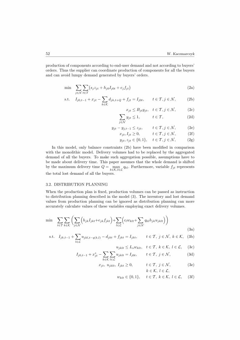
production of components according to end-user demand and not according to buyers’orders. Thus the supplier can coordinate production of components for all the buyersand can avoid lumpy demand generated by buyers’ orders.

min∑j∈N

∑t∈T

(sjzjt + hj0Ij0t + ejfjt

)(2a)

s.t. Ij0,t−1 + xjt −∑k∈K

djk,t+Q + fjt = Ij0t, t ∈ T , j ∈ N , (2b)

xjt ≤ Bjtyjt, t ∈ T , j ∈ N , (2c)∑j∈N

yjt ≤ 1, t ∈ T , (2d)

yjt − yj,t−1 ≤ zjt, t ∈ T , j ∈ N , (2e)xjt, Ijt ≥ 0, t ∈ T , j ∈ N , (2f)yjt, zjt ∈ {0, 1}, t ∈ T , j ∈ N , (2g)

In this model, only balance constraints (2b) have been modified in comparisonwith the monolithic model. Delivery volumes had to be replaced by the aggregateddemand of all the buyers. To make such aggregation possible, assumptions have tobe made about delivery time. This paper assumes that the whole demand is shiftedby the maximum delivery time Q = max

k∈K,l∈Lqkl. Furthermore, variable fjt represents

the total lost demand of all the buyers.

3.2. DISTRIBUTION PLANNING

When the production plan is fixed, production volumes can be passed as instructionto distribution planning described in the model (3). The inventory and lost demandvalues from production planning can be ignored as distribution planning can moreaccurately calculate values of these variables employing exact delivery volumes.

min∑t∈T

∑k∈K

(∑j∈N

(hjkIjkt+ejkfjkt

)+∑l∈L

(clwklt+

∑j∈N

qklhjkujklt

))(3a)

s.t. Ijk,t−1 +∑l∈L

ujkl,t−q(k,l) − djkt + fjkt = Ijkt, t ∈ T , j ∈ N , k ∈ K, (3b)

ujklt ≤ Lswklt, t ∈ T , k ∈ K, l ∈ L, (3c)

Ij0,t−1 + x∗jt −∑k∈K

∑l∈L

ujklt = Ij0t, t ∈ T , j ∈ N , (3d)

xjt, ujklt, Ijkt ≥ 0, t ∈ T , j ∈ N , (3e)k ∈ K, l ∈ L,

wklt ∈ {0, 1}, t ∈ T , k ∈ K, l ∈ L, (3f)


The only difference between the constraints in this model and in the monolithicmodel is in parameter x∗jt which represents production volumes calculated in theproduction model and is not subject to changes in the distribution model.

The above distribution planning problem cannot be solved separately for all thebuyers as they all depend on common production volumes, i.e. they share supplierscomponent inventories. After simultaneous planning of production for all the buyersthis may be seen as another form of coordination. However, the production anddistribution schedules continue to remain uncoordinated. Therefore, the sequentialmethod represents only a partial coordination approach.

3.3. TRADITIONAL METHOD

Traditional planning follows order reversed against the sequential method. First,all the buyers completely independently make joint replenishment decisions and sendorders to the supplier. The buyers take into account no suppliers’ capacity utilization,start-up costs of machines or orders from the other buyers.

Supplier has to adjust his production plan to the buyers’ orders. The only waythat the buyers can make this task for the supplier a little easier is to share with himthe information about planned replenishment orders as early as possible. This paperassumes that the supplier knows orders for the same horizon as end-user demandforecasts used in the monolithic and sequential methods.

4. DATA PARAMETERS

The objective of this study is to investigate the impact of the three planning methodson the overall supply chain cost at various parameters settings.

The data for two demand scenarios and truck characteristics have been collectedby Miodońska (2006) for the automotive industry. In all the scenarios, there are twocomponents, one supplier and three buyers, i.e. car manufacturers, practically in thesame distance to the supplier. The planning horizon is 30 days long, but effectiveplanning horizon is 2–3 days shorter due to long delivery times.

Truck characteristics are given in table 3 Note high variability of the fixedcost-capacity ratio.

Table 3. Characteristics of trucks (Miodonska 2006)

Truck Capacity–fixed cost ratio Delivery time(Ll/cl ∗ 100%) [days]

1 41% 22 100% 23 234% 34 290% 3

The second truck is the most frequently used and serves as a reference

54 W. Kaczmarczyk

In the study, 144 test problems are formed from two demand scenarios and all com-binations of the following parameters: lost demand unit cost ej ∈ {40, 400}, start-upcosts sj ∈ {50, 100, 200}, fixed delivery cost of the second truck c2 ∈ {125, 250, 500}(the most widely used), suppliers capacity utilization u ∈ {60%, 70%, 80%, 90%}.

Utilization u is defined as the total demand divided by capacity of 27 days availablefor production. Production on day 28 does not make any sense as the fastest truckneeds 2 days to deliver the components to any buyer.

The values of lost demand unit cost ej ∈ {40, 400} require some explanations.Higher value should actually prevent any lost demand in the solutions as its is higherthan the set-up cost for both production and delivery (with the smallest truck). Thus,high values do not have any economical justification. Smaller value will allow moreaccurate comparison of the results in a case when lost demand is inevitable.

In the practice of the automotive industry, both settings might be accurate.When the supplier plans his operations for the already accepted end-user demandvolumes, the indispensable inventory levels at the buyers’ sites must be guaranteed.On the other hand, the buyers, i.e. car manufacturers, sometimes face unexpectedshort-horizon demand fluctuations and ask suppliers to make deliveries earlier or todeliver more than previously agreed. Under such circumstances, the supplier has noobligation to deliver the ordered quantities but attempts to satisfy the buyers’ un-planned demand. That situation will be modelled by a smaller value of lost demandunit cost.

The unit processing time pj and the unit holding costs hjk have been set to 1 for allthe components and all the buyers. Therefore, the values of lost demand unit cost ej ,start-up costs sj and fixed delivery cost cl express also the ratio to unit holding cost.

5. EXPERIMENTAL RESULTS

All the three methods analyzed in this paper have been implemented in ILOG OPLDevelopment Studio 6.1 using ILOG CPLEX 11 to solve MIP problems (Fig. 1). Allthe test problems have been solved on a computer with the Intel T1300 1.66 MHzprocessor with 10 minutes time limit. In the decomposition methods productionplanning was solved optimally in less than a minute and the rest of time was spenton solving the distribution (replenishment) problem.

The percentage duality gap between the best integer solution f∗ and the linearrelaxation fR was calculated as (f∗ − fR)/fR. For the methods consisting of severalmodels, total f∗ and fR were calculated as a sum of f∗ and fR of all these models.The average values of duality gap are given in Figure 1. For the monolithic methodthey ranged from 20.2% to 36.5%, for the sequential method from 5.4% to 17.8%, andfor the traditional method from 0.8% to 8.6%.

The most dramatic effect visible in this figure is the high average duality gap of themonolithic method, equal to 29.1%. It is three times higher than for the sequentialmethod (10.7%) and six times higher than for the traditional method (4.9%).

Furthermore, if fixed delivery costs are high, the distribution problem becomesmore important and the traditional method is completed with a very small gap.


If fixed delivery costs are small, the sequential method has duality gap almost assmall as the traditional one. The suppliers’ start-up costs do not seem to have anysignificant impact on the complexity of the problem. These results are not surprising.Complexity of the monolithic model is much higher and in case of high delivery coststhe traditional method, which initially tries to minimize these costs, should achievebetter results.

Fig. 1. Average MIP duality gap at small lost demand unit costs

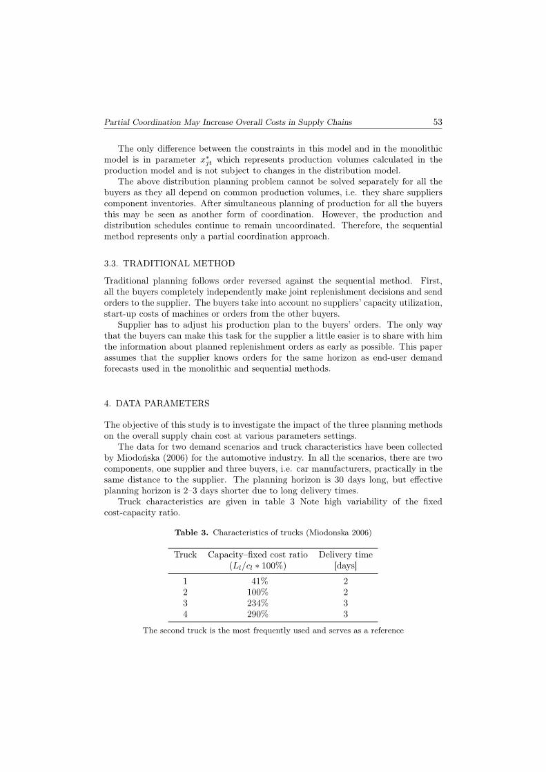
Figures 2 and 3 give values of all the cost factors of the entire supply chain. Thefirst figure gives average values for the test problems with small lost demand unit costas percentage ratio to the overall cost determined with the traditional method.

The most significant finding in Figure 2 is the average 17% decrease of overall costpossible with the monolithic method. The sequential method is also better than thetraditional one (in average by 6%).

Both decomposition methods guarantee small values of costs minimized in thefirst step of planning. The sequential method generated small start-up and inventorycosts, the traditional one produced small delivery costs.

The monolithic method surpasses the two other methods primarily in minimizinglost demand. It is a very good news for the supplier, as satisfaction of the buyer is atleast as important as the cost effect (assuming that the supplier is able to build andsolve the monolithic model).

56 W. Kaczmarczyk

Fig. 2. Total cost factors at small lost demand unit costs, as ratio to total cost obtainedwith the traditional method

Fig. 3. Total cost factors at high lost demand unit costs, as ratio to total cost obtainedwith the sequential method

Figure 3 presents cost values for the test problems with prohibitive lost demandcosts expressed as percentage ratio to the overall cost determined with the sequentialmethod. First of all, the traditional method fails to eliminate lost demand. Thiscannot be surprising as the traditional method completely ignores supplier capacitylimits while planning component deliveries. Furthers details are given in Figure 4.


Both methods implementing the VMI approach eliminate lost demand completely.It is interesting to compare their results without lost demand: delivery costs dominateall other cost factors then. Obviously, successful coordination requires much morefrequent deliveries with smaller trucks. However, the monolithic method results intwice as high inventories and a little lower start-up costs. Finally, the monolithicmethod guarantees on average 19% lower overall cost than of the sequential one.

Figure 4 presents when exactly the traditional method fails to eliminate lost de-mand. It seems that getting low lost demand with this method is only possible atsmall fixed delivery costs and low utilization. High costs and high utilization maylead even to 10% lost demand.

Fig. 4. Impact of suppliers’ capacity utilization and delivery fixed cost on percentage of lostdemand at high lost demand unit costs

Figures 5 and 6 present the relationship between the supply chain overall costand delivery fixed cost. Both charts present ratio of the overall supply chain costobtained with the given method to the overall cost obtained with the traditionalmethod. Figure 5 gives the results at small lost demand unit cost. It seems thatfixed delivery costs do not have significant impact except for the sequential method.This may be easily explained as this method ignores delivery cost in the first planningstep. When lost demand unit costs are high (see Fig. 6), the situation is completelydifferent. Now almost any change in unit costs significantly changes the total cost.

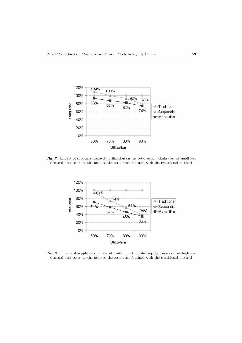
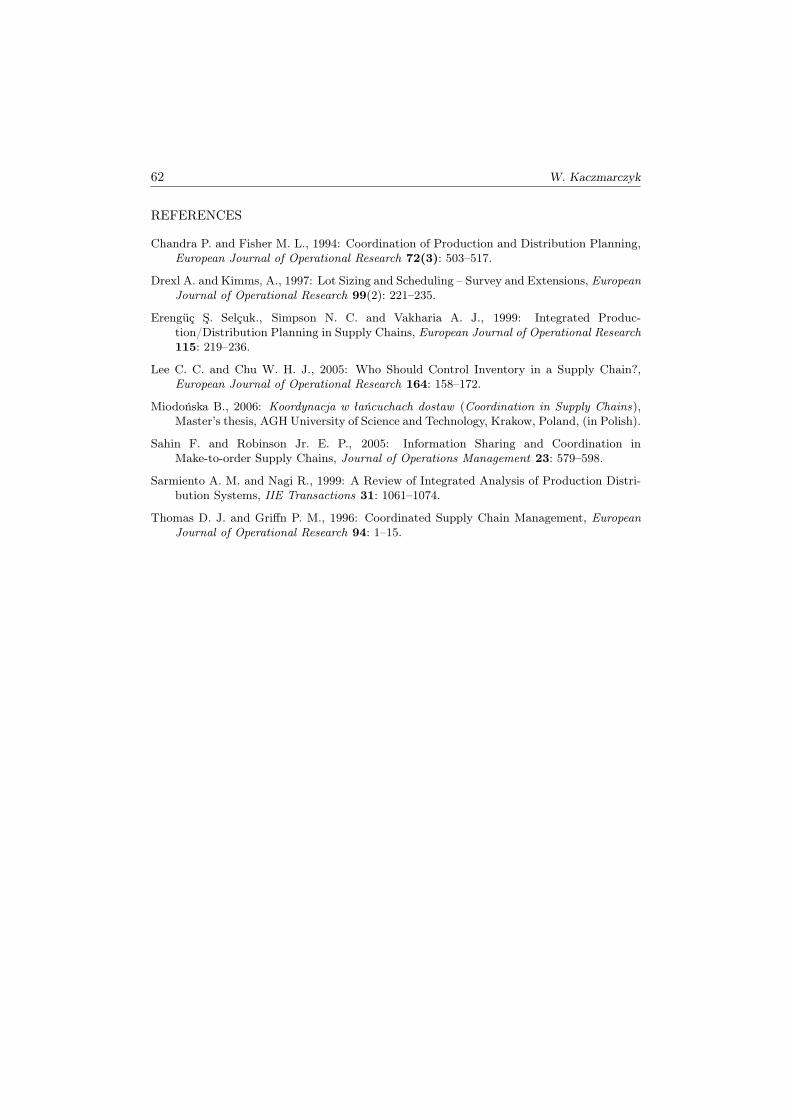
Figures 7 and 8 give the relationship between the total supply chain cost and thesupplier’ capacity utilization. The values of costs for all the methods are given as theratio to the costs obtained with the traditional method.

Figure 7 gives the results at small lost demand unit costs. This is probably themost interesting chart in this paper. It shows that for small utilization of suppliers’capacity (about 60%), the sequential method applying VMI approach gives 9% worseresults than the traditional method.

58 W. Kaczmarczyk

Fig. 5. Impact of delivery fixed cost on the total supply chain cost at small lost demandunit costs, as the ratio to the total cost obtained with the traditional method

Fig. 6. Impact of delivery fixed cost on the total supply chain cost at high lost demand unitcosts, as the ratio to the total cost obtained with the traditional method


Fig. 7. Impact of suppliers’ capacity utilization on the total supply chain cost at small lostdemand unit costs, as the ratio to the total cost obtained with the traditional method

Fig. 8. Impact of suppliers’ capacity utilization on the total supply chain cost at high lostdemand unit costs, as the ratio to the total cost obtained with the traditional method

60 W. Kaczmarczyk

For the suppliers of car components, it is a very bad news. On one hand, theyhave to accept low utilization of their resources to guarantee high customer service.On the other hand, they are forced to cooperate in VMI fashion. But under suchcircumstances, they obviously risk increase in their operational costs. This is exactlythe opposite of what should be expected. Coordination enabled by VMI contractsintends to decrease operational costs and not to increase them.

The good news is that for low utilization the traditional method is not much worsethan the monolithic one, with only 7% difference. Similarly, for high utilization, thesequential method seems to be almost as good as the monolithic one. The differenceis only 4% and both VMI methods yield much better results than the traditional one.The sequential method is 22% better and the monolithic one as much as 26%.

The general tendencies are easy to explain. The traditional method starts withminimizing distribution costs which are dominant in case of low utilization of suppli-ers’ resources. In the opposite case, the production schedule is more important andthat is why the sequential method minimizing first that part of the problem is betterfor high utilization.

If lost demand unit cost is high (see Fig. 8), the chart looks very similar withthe difference that all values of the VMI methods are always better than those of thetraditional method. For small utilization, the improvement is only 6%.

The relationship between lost demand and fixed delivery cost at small lost demandunit costs is given in Figure 9. As expected, lost demand increases when delivery costincreases. A little surprising is the high value for the sequential method and highdelivery costs.

Fig. 9. Impact of delivery fixed cost on percentage of lost demand at small lost demandunit costs


The relationship between lost demand and suppliers’ capacity utilization is givenin Figure 10. As expected, increasing suppliers’ utilization increases volume of lostdemand, more for the traditional method than for the monolithic one. The resultsfor the sequential method are counterintuitive, but this negative relationship is veryweek and almost negligible.

Fig. 10. Impact of suppliers capacity utilization on percentage of lost demand at small lostdemand unit costs

6. CONCLUSION

The paper analyses operational coordination of production and distribution within anindustrial supply chain. Using the Mixed Integer Programming models, three differentplanning methods have been studied, one emulating the traditional way of planningand two applying the Vendor Managed Inventory (VMI) approach. The former solvedmonolithic model of the integrated problem, the latter copied the procedures appliedin the imperfect VMI practice. All the methods have been tested on several data setsfor a variety of parameters .

The general conclusion is that selection of the planning method is very importantand depends on actual parameter settings. For low utilization of suppliers’ resources,the traditional method is not much worse than the monolithic one. For high utiliza-tion, the sequential method achieves very good results. As expected, the monolithicmethod is best in all cases. It is however much more complex what makes practicalapplications very hard.

Another conclusion is that for low utilization the sequential method may lead toincrease in the overall cost in comparison with the traditional method. This is veryimportant, because suppliers of components have often to accept low utilization oftheir resources to guarantee high customer service. They are also forced by the buyersto cooperate in the VMI fashion. Under such circumstances, the suppliers have tomake an effort to develop full coordination procedures similarly to the monolithicmethod.

62 W. Kaczmarczyk

REFERENCES

Chandra P. and Fisher M. L., 1994: Coordination of Production and Distribution Planning,European Journal of Operational Research 72(3): 503–517.

Drexl A. and Kimms, A., 1997: Lot Sizing and Scheduling – Survey and Extensions, EuropeanJournal of Operational Research 99(2): 221–235.

Erengüç Ş. Selçuk., Simpson N. C. and Vakharia A. J., 1999: Integrated Produc-tion/Distribution Planning in Supply Chains, European Journal of Operational Research115: 219–236.

Lee C. C. and Chu W. H. J., 2005: Who Should Control Inventory in a Supply Chain?,European Journal of Operational Research 164: 158–172.

Miodońska B., 2006: Koordynacja w łańcuchach dostaw (Coordination in Supply Chains),Master’s thesis, AGH University of Science and Technology, Krakow, Poland, (in Polish).

Sahin F. and Robinson Jr. E. P., 2005: Information Sharing and Coordination inMake-to-order Supply Chains, Journal of Operations Management 23: 579–598.

Sarmiento A. M. and Nagi R., 1999: A Review of Integrated Analysis of Production Distri-bution Systems, IIE Transactions 31: 1061–1074.

Thomas D. J. and Griffn P. M., 1996: Coordinated Supply Chain Management, EuropeanJournal of Operational Research 94: 1–15.

partial coordination may increase overall costs in supply...

Documents