Partial Differential Equations andMonge–Kantorovich Mass Transfer

Lawrence C. Evans∗

Department of MathematicsUniversity of California, Berkeley

September, 2001 version

1. Introduction1.1 Optimal mass transfer1.2 Relaxation, duality

Part I: Cost = 12(Distance)2

2. Heuristics2.1 Geometry of optimal transport2.2 Lagrange multipliers

3. Optimal mass transport, polar factorization3.1 Solution of dual problem3.2 Existence of optimal mass transfer plan3.3 Polar factorization of vector fields

4. Regularity4.1 Solving the Monge–Ampere equation4.2 Examples4.3 Interior regularity for convex targets4.4 Boundary regularity for convex domain and target

5. Application: Nonlinear interpolation6. Application: Time-step minimization and nonlinear diffusion

6.1 Discrete time approximation6.2 Euler–Lagrange equation

∗Supported in part by NSF Grant DMS-94-24342. This paper appeared in Current Developments inMathematics 1997, ed. by S. T. Yau

1

6.3 Convergence7. Application: Semigeostrophic models in meteorology

7.1 The PDE in physical variables7.2 The PDE in dual variables7.3 Frontogenesis

Part II: Cost = Distance

8. Heuristics8.1 Geometry of optimal transport8.2 Lagrange multipliers

9. Optimal mass transport9.1 Solution of dual problem9.2 Existence of optimal mass transfer plan9.3 Detailed mass balance, transport density

10. Application: Shape optimization11. Application: Sandpile models

11.1 Growing sandpiles11.2 Collapsing sandpiles11.3 A stochastic model

12. Application: Compression molding

Part III: Appendix

13. Finite-dimensional linear programming

References

In Memory ofFrederick J. Almgren, Jr.

andEugene Fabes

2

1 Introduction

These notes are a survey documenting an interesting recent trend within the calculus ofvariations, the rise of differential equations techniques for Monge–Kantorovich type optimalmass transfer problems. I will discuss in some detail a number of recent papers on variousaspects of this general subject, describing newly found applications in the calculus of vari-ations itself and in physics. An important theme will be the rather different analytic andgeometric tools for, and physical interpretations of, Monge–Kantorovich problems with auniformly convex cost density (here exemplified by c(x, y) = 1

2|x − y|2) versus those prob-

lems with a nonuniformly convex cost (exemplified by c(x, y) = |x − y|). We will as wellstudy as applications several physical processes evolving in time, for which we can identifyoptimal Monge–Kantorovich mass transferences on “fast” time scales.

The current text corrects some minor errors in earlier versions, improves the expositiona bit, and adds a few more references. The interested reader may wish to consult as well thelecture notes of Urbas [U1] and of Ambrosio [Am] for more.

1.1 Optimal mass transfer

The original transport problem, proposed by Monge in the 1780’s, asks how best to move apile of soil or rubble (“deblais”) to an excavation or fill (“remblais”), with the least amountof work. In modern parlance, we are given two nonnegative Radon measures µ± on Rn,satisfying the overall mass balance condition

µ+(Rn) = µ−(Rn) <∞, (1.1)

and we consider the class of measurable, one-to-one mappings s : Rn → Rn which rearrange

µ+ into µ−:

s#(µ+) = µ−. (1.2)

In other words, we require ∫X

h(s(x)) dµ+(x) =

∫Y

h(y) dµ−(y) (1.3)

for all continuous functions h, where X = spt(µ+), Y = spt(µ−). We denote by A theadmissible class of mappings s as above, satisfying (1.2), (1.3)

Given also is the work or cost density function

c : Rn × Rn → [0,∞);

3

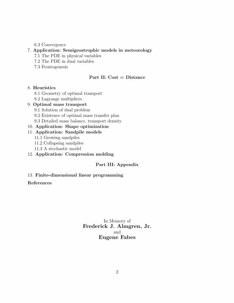
so that c(x, y) records the work required to move a unit mass from the position x ∈ Rn toa new position y ∈ Rn. (In Monge’s original problem c(x, y) = |x − y|; that is, the work issimply proportional to the distance moved.)

s

X=spt(µ+) Y=spt(µ-)

The total work corresponding to a mass rearrangement plan s ∈ A is thus

I[s] :=

∫Rn

c(x, s(x)) dµ+(x). (1.4)

Our problem is therefore to find and characterize an optimal mass transfer s∗ ∈ A whichminimizes the work:

I[s∗] = mins∈A

I[s]. (1.5)

In other words, we wish to construct a one-to-one mapping s∗ : Rn → Rn which pushes the

measure µ+ onto µ− and, among all such mappings, minimizes I[·]. We will later see that areally remarkable array of interesting mathematical and physical interpretations follow.

This is even now, over two hundred years later, a difficult mathematical problem, owingmostly to the highly nonlinear structure of the constraint. For instance, if µ± have smoothdensities f±, that is, if

dµ+ = f+dx, dµ− = f−dy, (1.6)

then (1.2) reads

f+(x) = f−(s(x))det(Ds(x)) (x ∈ X), (1.7)

where we write s = (s1, . . . , sn) and

Ds =

s1x1

. . . s1xn

. . .

snx1

. . . snxn

n×n

= Jacobian matrix of the mapping s.

4

It is not at all apparent offhand that there exists any mapping, much less an optimalmapping, satisfying this constraint. Additionally, if {sk}∞k=1 ⊂ A is a minimizing sequence,

I[sk]→ infs∈A

I[s],

an obvious guess is that we can somehow pass to a subsequence {skj}∞j=1 ⊂ {sk}∞k=1, which

in turn converges to an optimal mass allocation plan s∗:

skj→ s∗.

However, there is no clear way to extract such a subsequence, converging in any reasonablesense to a limit. The direct methods of the calculus of variations fail spectacularly, asthere are no terms creating any sort of compactness built into the work functional I[·]. Inparticular, I[·] does not involve the gradient of s at all and so is not coercive on any Sobolevspace. And yet, as we will momentarily see, precisely this feature opens up the problem tomethods of linear programming.

1.2 Relaxation, duality

Kantorovich in the 1940’s [K1],[K2] (see also [R]) resolved certain of these problems byintroducing:

(i) a “relaxed” variant of Monge’s original mass allocation problemand, more importantly,

(ii) a dual variational principle.

The idea behind (i) is, remarkably, to transform (1.5) into a linear problem. The trick isfirstly to introduce the class

M :={Radon probability measures µ on Rn × Rn | projxµ = µ+, projyµ = µ−

}(1.8)

of measures on the product space Rn×Rn, whose projections on the first n coordinates andthe last n coordinates are, respectively, µ+, µ−. Given then µ ∈ M, we define the relaxedcost functional

J [µ] :=

∫Rn×Rn

c(x, y) dµ(x, y). (1.9)

The point of course is that if we have a mapping s ∈ A, then the induced measure

µ(E) := µ+{x ∈ Rn | (x, s(x)) ∈ E} (E ⊂ Rn × Rn, E Borel) (1.10)

5

belongs toM. Furthermore the new functional (1.9) is linear in µ and so, under appropriateassumptions on the cost c, simple compactness arguments assert the existence of at least oneoptimal measure µ∗ ∈M, satisfying

J [µ∗] = minµ∈M

J [µ]. (1.11)

Such a measure µ∗ need not, however, be generated by any one-to-one mapping s ∈ A, andconsequently the foregoing construction allows us only to establish the existence of a “weak”or “generalized” solution of Monge’s original problem. We will several times later return tothe central problem of fashioning some sort of “strong” solution, which actually correspondsto a mapping.

Of even greater importance for our purposes was Kantorovich’s additional introduction ofa dual problem. The best way to motivate this is by analogy with the finite dimensional case.Suppose that then cij, µ

+i , µ−j (i = 1, . . . , n; j = 1, . . . , m) are given nonnegative numbers,

satisfying the balance conditionn∑

i=1

µ+i =

m∑j=1

µ−j ,

and we wish to find µ∗ij (i = 1, . . . , n; j = 1, . . . , m) to

minimizen∑

i=1

m∑j=1

cijµij, (1.12)

subject to the constraints

m∑j=1

µij = µ+i ,

n∑i=1

µij = µ−j , µij ≥ 0 (i = 1, . . . , n; j = 1, . . . , m). (1.13)

This is clearly the discrete analogue of (1.8), (1.9), (1.11). As explained in the appendix(§13) the discrete linear programming dual problem to (1.12) is to find u = (u1, . . . , un) ∈ Rn,v = (v1, . . . , vm) ∈ Rm so as to

maximizen∑

i=1

uiµ+i +

m∑j=1

vjµ−j , (1.14)

subject to the inequalities

ui + vj ≤ cij (i = 1, . . . , n; j = 1, . . . , m). (1.15)

We can now by analogy guess the dual variational principle to (1.11). For this, weintroduce a continuous variant of (1.15) by defining

L := {(u, v) | u, v : Rn → R continuous, u(x) + v(y) ≤ c(x, y) (x, y ∈ Rn)}.(1.16)

6

Likewise, we introduce the continuous analogue of (1.14) by setting

K[u, v] :=

∫Rn

u(x) dµ+(x) +

∫Rn

v(y) dµ−(y). (1.17)

Consequently our dual problem is to find an optimal pair (u∗, v∗) ∈ L such that

K[u∗, v∗] = max(u,v)∈L

K[u, v]. (1.18)

In summary then, the transformation of Monge’s original mass allocation problem (1.5)into the dual problem (1.18) presents us with a rather different vantage point: rather thanstruggling to construct an optimal mapping s∗ ∈ A satisfying a highly nonlinear constraint,we are now confronted with the task of finding an optimal pair (u∗, v∗) ∈ L. And this, aswe will see later, is really easy. The mathematical structure of the dual problem providesprecisely what was missing for the original problem, enough compactness to construct aminimizer as some sort of limit of a minimizing sequence.

And yet this of course is not the story’s end. Kantorovich’s methods of first relaxing andthen dualizing have brought us into a realm where routine mathematical tools work, buthave also taken us far away from the original issue: namely, how do we actually fashion anoptimal allocation plan s∗?

We devote much of the remainder of the paper to answering this question, in two mostimportant cases of the uniformly convex cost density:

c(x, y) =1

2|x− y|2 (x, y ∈ Rn), (1.19)

and the nonuniformly convex cost density

c(x, y) = |x− y| (x, y ∈ Rn). (1.20)

These “L2” and “L1” theories are rich in mathematical structure, and serve as archetypesfor other models. Observe carefully the very different geometric consequences: in the firstcase the graph of the mapping y �→ c(x, y) contains no straight lines, and in the second caseit does. The latter degeneracy will create interesting problems.

Remark. I make no attempt in this paper to survey the vast literature on Monge–Kantorovich methods in probability and statistics, a nice summary of which may be foundin Rachev [R]. ✷

Part I: Cost = 12(Distance)2

7

2 Heuristics

For this and the next five sections we take the quadratic cost density

c(x, y) :=1

2|x− y|2 (x, y ∈ Rn), (2.1)

| · | denoting the usual Euclidean norm. We hereafter wish to understand if and how we canconstruct an optimal mass transfer plan s∗ solving (1.5), where now

I[s] :=1

2

∫Rn

|x− s(x)|2 dµ+(x) (2.2)

for s in A, the admissible class of measurable, one-to-one maps of Rn which push forwardthe measure µ+ to µ−. The following techniques were largely pioneered by Y. Brenier in[B2].

2.1 Geometry of optimal transport

We begin with some informal insights, our goal being to understand, for the moment withoutproofs, what information about an optimal mapping we can extract directly from the originaland dual variational principles. In other words, how can we exploit the very fact that a givenmapping minimizes the work functional I[·] (among all other mappings in A), to understandits precise geometric properties?

So now let us assume that s∗ ∈ A minimizes the work functional (2.2), among all othermappings s ∈ A. Fix a positive integer m, take distinct points {xk}mk=1 ⊂ X = spt (µ+),and assume we can find small disjoint balls

Ek := B(xk, rk) (k = 1, . . . , m), (2.3)

and radii {rk}mk=1, adjusted so that

µ+(E1) = · · · = µ+(Em) = ε. (2.4)

Next write yk := s∗(xk), Fk := s∗(Ek). Since s∗ pushes µ+ to µ−, we have

µ−(F1) = · · · = µ−(Fm) = ε. (2.5)

We construct another mapping s ∈ A by cyclically permuting the images of the balls{Ek}mk=1. That is, we design s ∈ A so that

s(xk) = yk+1, s(Ek) = Fk+1 (k = 1, . . . , m)

s ≡ s∗ on X −m⋃

k=1

Ek,(2.6)

8

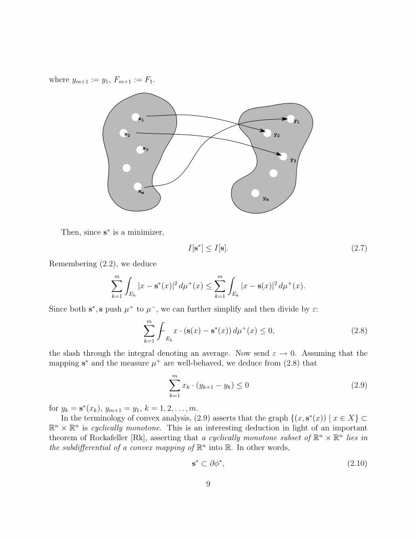
where ym+1 := y1, Fm+1 := F1.

x1

x2

x3

xm

y2

y1

y3

ym

Then, since s∗ is a minimizer,

I[s∗] ≤ I[s]. (2.7)

Remembering (2.2), we deduce

m∑k=1

∫Ek

|x− s∗(x)|2 dµ+(x) ≤m∑

k=1

∫Ek

|x− s(x)|2 dµ+(x).

Since both s∗, s push µ+ to µ−, we can further simplify and then divide by ε:

m∑k=1

∫−

Ek

x · (s(x)− s∗(x)) dµ+(x) ≤ 0, (2.8)

the slash through the integral denoting an average. Now send ε → 0. Assuming that themapping s∗ and the measure µ+ are well-behaved, we deduce from (2.8) that

m∑k=1

xk · (yk+1 − yk) ≤ 0 (2.9)

for yk = s∗(xk), ym+1 = y1, k = 1, 2, . . . , m.In the terminology of convex analysis, (2.9) asserts that the graph {(x, s∗(x)) | x ∈ X} ⊂

Rn × Rn is cyclically monotone. This is an interesting deduction in light of an important

theorem of Rockafeller [Rk], asserting that a cyclically monotone subset of Rn × Rn lies inthe subdifferential of a convex mapping of Rn into R. In other words,

s∗ ⊂ ∂φ∗, (2.10)

9

for some convex function φ∗, in the sense of possibly multivalued graphs on Rn×Rn. More-over, a convex function is differentiable a.e., and so

s∗ = Dφ∗ a.e. in X, (2.11)

where D denotes the gradient.We have come upon an important deduction: an optimal mass allocation plan is the

gradient of a convex potential φ∗. (Cf. McCann [MC2], etc.)

2.2 Lagrange multipliers

In view of its importance we provide next an alternative, but still strictly formal, analyticderivation of (2.11).

For this, we assume the measures µ± have smooth densities, dµ+ = f+dx, dµ− = f−dy,and introduce the augmented work functional

I[s] :=

∫Rn

1

2|x− s(x)|2f+(x) + λ(x)[f−(s(x))det(Ds(x))− f+(x)]dx,

(2.12)

where the function λ is the Lagrange multiplier corresponding to the pointwise constraintthat s#(µ+) = µ− (that is, f+ = f−(s)det(Ds)). Computing the first variation, we find fork = 1, . . . , m:

(λf−(s∗)(cofDs∗)ki )xi

= (s∗k − xk)f+ + λf−yk

(s∗)det(Ds∗). (2.13)

Here cofDs∗ is the cofactor matrix of Ds∗; that is, the (k, i)th entry of cofDs∗ is (−1)k+i

times the (k, i)th minor of the matrix Ds∗.Standard matrix identities assert (cofDs∗)k

i,xi= 0, s∗lxi

(cofDs∗)ki = δkl(detDs∗), and

s∗kxj(cofDs∗)k

i = δij(detDs∗). We employ these equalities to simplify (2.13), and therebydiscover after some calculations

λxif−(s∗)(cofDs∗)k

i = (s∗k − xk)f+. (2.14)

Now multiply by s∗kxjand sum on k, to deduce:

λxj= (s∗k − xk)s

∗kxj

.

But then (λ− |s

∗ − x|22

+|x|22

)xj

= s∗j (j = 1, . . . , n),

and so (2.11) again follows, for the potential φ∗ := λ− |s∗−x|22

+ |x|22

.

10

3 Optimal mass transport, polar factorization

3.1 Solution of dual problem

The foregoing heuristics done with, we turn next to the task of proving rigorously the exis-tence of an optimal mass allocation plan. We expect s∗ = Dφ∗ almost everywhere for someconvex potential φ∗, and the task is now really to deduce this. We will do so from the Kan-torovich dual variational principle (1.16)– (1.18) introduced in §1. We hereafter concentrateon the situation

dµ+ = f+dx, dµ− = f−dy, (3.1)

where f± are bounded, nonnegative functions with compact support, satisfying the massbalance condition ∫

X

f+(x)dx =

∫Y

f−(y) dy (3.2)

where, as always, X := spt (f+), Y := spt (f−). For the case at hand, the dual problem isto find (u∗, v∗) so as to maximize

K[u, v] :=

∫X

u(x)f+(x) dx +

∫Y

v(y)f−(y) dy, (3.3)

subject to the constraint

u(x) + v(y) ≤ 1

2|x− y|2 (x ∈ X, y ∈ Y ). (3.4)

We wish to take up tools from convex analysis, and for this must first change variables:{φ(x) := 1

2|x|2 − u(x) (x ∈ X)

ψ(y) := 12|y|2 − v(y) (y ∈ Y ).

(3.5)

Note that now (3.4) says

φ(x) + ψ(y) ≥ x · y (x ∈ X, y ∈ Y ), (3.6)

and so the variational problem is then to minimize

L[φ, ψ] :=

∫X

φ(x)f+(x) dx +

∫Y

ψ(y)f−(y) dy, (3.7)

subject to the constraint (3.6).

11

Lemma 3.1 (i) There exist (φ∗, ψ∗) solving this minimization problem.(ii) Furthermore, (φ∗, ψ∗) are dual convex functions, in the sense that{

φ∗(x) = maxy∈Y

(x · y − ψ∗(y)) (x ∈ X)

ψ∗(y) = maxx∈X

(x · y − φ∗(x)) (y ∈ Y ).(3.8)

Proof. 1. If φ, ψ satisfy (3.6), then

φ(x) ≥ maxy∈Y

(x · y − ψ(y)) =: φ(x) (3.9)

and

φ(x) + ψ(y) ≥ x · y (x ∈ X, y ∈ Y ). (3.10)

Consequently

ψ(y) ≥ maxx∈X

(x · y − φ(x)) =: ψ(y) (3.11)

and

φ(x) + ψ(y) ≥ x · y (x ∈ X, y ∈ Y ). (3.12)

As ψ ≥ ψ, (3.9) impliesmaxy∈Y

(x · y − ψ(y)) ≥ φ(x).

This and (3.12) say

φ(x) = maxy∈Y

(x · y − ψ(y)). (3.13)

Since f± ≥ 0 and ψ ≥ ψ, φ ≥ φ, we see that L[φ, ψ] ≤ L[φ, ψ].2. Consequently in seeking for minimizers of L we may restrict attention to convex dual

pairs (φ, ψ), as above. Such functions are uniformly Lipschitz continuous, and so, afteradding or subtracting constants, we can extract a uniformly convergent subsequence fromany minimizing sequence for L. We thereby secure an optimal, convex dual pair. ✷

3.2 Existence of optimal mass transfer plan

Let us now regard (3.8) as defining φ∗(x), ψ∗(y) for all x, y ∈ Rn. Then φ∗, ψ∗ : Rn → R areconvex, and consequently differentiable a.e. We demonstrate next that

s∗(x) := Dφ∗(x) (a.e. x ∈ X) (3.14)

solves the mass allocation problem.

12

Theorem 3.1 Define s∗ by (3.14). Then(i) s∗ : X → Y is essentially one-to-one and onto.

(ii)∫

Xh(s∗(x)) dµ+(x) =

∫Y

h(y) dµ−(y) for each h ∈ C(Y ).

(iii) Lastly,1

2

∫X

|x− s∗(x)|2 dµ+(x) ≤ 1

2

∫X

|x− s(x)|2 dµ+(x)

for all s : X → Y such that s#(µ+) = µ−.

Proof. 1. From the max-representation function (3.8) we see that s∗ = Dφ∗ ∈ Y a.e.2. Fix τ > 0, and define the variations{

ψτ (y) := ψ∗(y) + τh(y) (y ∈ Y )

φτ (x) := maxy∈Y

(x · y − ψτ (y)) (x ∈ X). (3.15)

Then

φτ (x) + ψτ (y) ≥ x · y (x ∈ X, y ∈ Y ) (3.16)

and soL[φ∗, ψ∗] ≤ L[φτ , ψτ ] =: i(τ).

As the mapping τ �→ i(τ) thus has a minimum at τ = 0,

0 ≤ 1

τ(L[φτ , ψτ ]− L[φ∗, ψ∗])

=

∫X

[φτ (x)− φ∗(x)

τ

]f+(x) dx +

∫Y

h(y)f−(y) dy.(3.17)

Now∣∣φτ−φ∗

τ

∣∣ ≤ ‖h‖L∞ . Furthermore if we take yτ ∈ Y so that

φτ (x) = x · yτ − ψτ (yτ ), (3.18)

then

φτ (x)− φ∗(x) = x · yτ − ψ∗(yτ )− τh(yτ )− φ∗(x) ≤ −τh(yτ ). (3.19)

On the other hand, if we select y ∈ Y such that

φ∗(x) = x · y − ψ∗(y), (3.20)

then

φτ (x)− φ∗(x) ≥ x · y − ψ∗(y)− τh(y)− φ∗(x) = −τh(y). (3.21)

13

Thus

− h(y) ≤ φτ (x)− φ∗(x)

τ≤ −h(yτ ). (3.22)

If we take a point x ∈ X where s∗(x) := Dφ∗(x) exists, then (3.20) implies y = s∗(x).Furthermore as τ → 0, yτ → s∗(x). Thus (3.17), (3.22) and the Dominated ConvergenceTheorem imply ∫

X

h(s∗(x))f+(x) dx ≤∫

Y

h(y)f−(y) dy.

Replacing h by −h, we deduce that equality holds. This is statement (ii).3. Now take s to be any admissible mapping. Then∫

X

ψ∗(s(x))f+(x) dx =

∫Y

ψ∗(y)f−(y) dy.

Since φ∗(x) + ψ∗(y) ≥ x · y, with equality for y = s∗(x), we consequently have

0 ≥∫

X[x · (s(x)− s∗(x))− φ∗(x) + φ∗(x)]f+(x) dx

=∫

X[x · (s(x)− s∗(x))]f+(x) dx.

This implies assertion (iii) of the Theorem: s∗ is optimal. ✷

This proof follows Gangbo [G] and Caffarelli [C4]. Another neat approach is due toMcCann [MC2]; he approximates the measures µ± by point masses, solves the resultingdiscrete linear programming problem, and the passes to limits. See also Gangbo–McCann[G-M1], [G-M2], McCann [MC4]. An interesting related work is Wolfson [W].

3.3 Polar factorization of vector fields

Assume next that U ⊂ Rn is open, bounded, with |∂U | = 0, and that r : U → Rn is a

bounded measurable mapping satisfying the nondegeneracy condition{|r−1(N)| = 0 for each bounded Borelset N ⊂ Rn, with |N | = 0.

(3.23)

Define the modified functional

L[φ, ψ] :=

∫U

φ(r(y)) + ψ(y) dy, (3.24)

which we propose to minimize among functions (φ, ψ) satisfying

φ(x) + ψ(y) ≥ x · y. (3.25)

14

Let (φ∗, ψ∗) solve this problem. Then taking variations as in the previous proof, we deduce∫U

h(y) dy =

∫U

h(Dφ∗(r(y)) dy

for all h ∈ C(U). Define nows∗(x) := Dφ∗(r(x)).

Then s∗ is measure preserving and

r(x) = Dψ∗(s∗(x)). (3.26)

This is the polar factorization of the vector field r, as the composition of the gradient of aconvex function and a measure preserving mapping. ✷

This remarkable polar factorization was established by Brenier [B1], [B2], and the prooflater simplified by Gangbo [G]. (Brenier was motivated by problems in fluid mechanics,which we will not discuss in this paper: see [B3].)

Remark. We can regard (3.26) as a nonlinear generalization of the Helmholtz decom-position of a vector field into the sum of a gradient and a divergence-free field. To see thisformally, let a be a given vector field and write

r0 := id, s0 := id, ψ0 :=|x|22

.

Set

r(τ) := r0 + τa (3.27)

for small |τ |. The polar factorization gives

r(τ) := Dψ(τ) ◦ s(τ), (3.28)

where ψ(τ) is convex, s(τ) is measure preserving, and we drop the superscript ∗. Next put

ψ(τ) = ψ0 + τb(τ), s(τ) = s0 + τc(τ) (3.29)

into (3.28), differentiate with respect to τ , and set τ = 0. We deduce

a = Db + c, (3.30)

for b = b(0), c = c(0). This is a Helmholtz decomposition of a, since

1 = det(Ds(τ)) = 1 + τdiv c + O(τ 2) (3.31)

implies div c = 0. ✷

15

4 Regularity

4.1 Solving the Monge–Ampere equation

The mass allocation problem solved in §3 can be interpreted as providing a weak or gener-alized solution to the Monge–Ampere PDE mapping problem:{

(a) f−(Dφ(x))detD2φ(x) = f+(x) (x ∈ X)(b) Dφ maps X into Y .

(4.1)

Now and hereafter we omit the superscript ∗. Recall that we interpret (4.1)(a) to mean∫X

h(Dφ(x))f+(x) dx =

∫Y

h(y)f−(y) dy (4.2)

for each continuous function h.There are, however, subtleties here. First of all, recall that since φ is convex, we can

interpret D2φ as a matrix of signed measures, which have absolutely continuous and singularparts with respect to Lebesgue measure:

d[D2φ] = [D2φ]ac dx + d[D2φ]s (4.3)

(see for instance [E-G2]). We say φ is a solution of

f−(Dφ)det(D2φ) = f+ (4.4)

in the sense of Alexandrov if the identity (4.2) holds, and additionally

d[D2φ]s = 0, φ is strictly convex. (4.5)

4.2 Examples

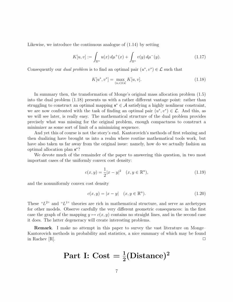
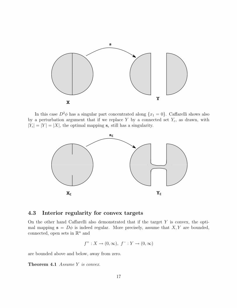
But, as noted by L. Caffarelli [C5], the solution constructed in §3 need not solve (4.4) inthe Alexandrov sense. Consider first of all the situation that n = 2 and X is the unit diskB(0, 1). Then s = Dφ, for

φ(x1, x2) = |x1|+1

2(x2

1 + x22),

optimally rearranges µ+ = χXdx into µ− = χY dy, where

Y = {(x1, x2) | 0 ≤ (x1 − 1)2 + x22, x1 ≥ 1}

∪ {(x1, xn) | 0 ≤ (x1 + 1)2 + x22, x1 ≤ −1}.

16

s

XY

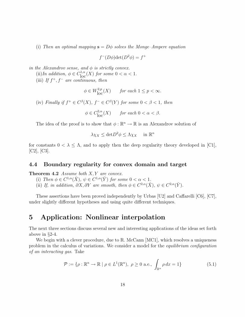
In this case D2φ has a singular part concentrated along {x1 = 0}. Caffarelli shows alsoby a perturbation argument that if we replace Y by a connected set Yε, as drawn, with|Yε| = |Y | = |X|, the optimal mapping sε still has a singularity.

sε

Xε Yε

4.3 Interior regularity for convex targets

On the other hand Caffarelli also demonstrated that if the target Y is convex, the opti-mal mapping s = Dφ is indeed regular. More precisely, assume that X, Y are bounded,connected, open sets in Rn and

f+ : X → (0,∞), f− : Y → (0,∞)

are bounded above and below, away from zero.

Theorem 4.1 Assume Y is convex.

17

(i) Then an optimal mapping s = Dφ solves the Monge–Ampere equation

f−(Dφ)det(D2φ) = f+

in the Alexandrov sense, and φ is strictly convex.(ii)In addition, φ ∈ C1,α

loc(X) for some 0 < α < 1.

(iii) If f+, f− are continuous, then

φ ∈ W 2,p

loc(X) for each 1 ≤ p <∞.

(iv) Finally if f+ ∈ Cβ(X), f− ∈ Cβ(Y ) for some 0 < β < 1, then

φ ∈ C2,α

loc(X) for each 0 < α < β.

The idea of the proof is to show that φ : Rn → R is an Alexandrov solution of

λχX ≤ detD2φ ≤ ΛχX in Rn

for constants 0 < λ ≤ Λ, and to apply then the deep regularity theory developed in [C1],[C2], [C3].

4.4 Boundary regularity for convex domain and target

Theorem 4.2 Assume both X, Y are convex.(i) Then φ ∈ C1,α(X), ψ ∈ C1,α(Y ) for some 0 < α < 1.(ii) If, in addition, ∂X, ∂Y are smooth, then φ ∈ C2,α(X), ψ ∈ C2,α(Y ).

These assertions have been proved independently by Urbas [U2] and Caffarelli [C6], [C7],under slightly different hypotheses and using quite different techniques.

5 Application: Nonlinear interpolation

The next three sections discuss several new and interesting applications of the ideas set forthabove in §2-4.

We begin with a clever procedure, due to R. McCann [MC1], which resolves a uniquenessproblem in the calculus of variations. We consider a model for the equilibrium configurationof an interacting gas. Take

P := {ρ : Rn → R | ρ ∈ L1(Rn), ρ ≥ 0 a.e.,

∫Rn

ρ dx = 1} (5.1)

18

to be the collection of mass densities, and to each ρ ∈ P associate the energy

E(ρ) :=

∫Rn

ργ(x) dx +

∫Rn

∫Rn

ρ(x)V (x− y)ρ(y) dxdy. (5.2)

The first term

E1(ρ) :=

∫Rn

ργ(x) dx

represents the internal energy, where γ > 1 is a constant. The second expression

E2(ρ) :=

∫Rn

∫Rn

ρ(x)V (x− y)ρ(y) dxdy

corresponds to the potential energy owing to interaction, where V : Rn → R is nonnegativeand strictly convex.

Suppose now ρ0, ρ1 ∈ P are both minimizers:

E(ρ0) = E(ρ1) = minρ∈P

E(ρ). (5.3)

A basic question concerns the uniqueness of these minimizers, up to translation invari-ance. Now the usual procedure would be to take the linear interpolation of ρ0, ρ1 and to askif the mapping t �→ E((1− t)ρ1 + tρ0) is convex on [0, 1]. This is however false in general forthe example at hand. McCann instead employs the ideas of §2–3 to build a sort of “nonlinearinterpolation” between ρ0, ρ1. His idea is to take the convex potential φ such that

s#(ρ0) = ρ1, (5.4)

where

s = Dφ. (5.5)

Define then

ρt := ((1− t)id + ts)#ρ0 (0 ≤ t ≤ 1). (5.6)

This nonlinear interpolation between ρ0 and ρ1 in effect locates a realm of convexity forE.

Theorem 5.1 The mapping t �→ E(ρt) is convex on [0, 1], and is strictly convex unless ρ1

is a translate of ρ0.

19

Proof. 1. We first compute

E2(ρt) =

∫Rn

∫Rn

ρt(x)V (x− y)ρt(y) dxdy

=

∫Rn

∫Rn

ρ0(x)V ((1− t)(x− y) + t(s(x)− s(y))ρ0(y) dxdy.(5.7)

As V is convex, the mapping t �→ E2(ρt) is convex.2. Next, (5.6) implies

E1(ρt) =

∫Rn

ργt (x) dx

=

∫Rn

[ρ0

det[(1− t)I + tDs]

]γ

det[(1− t)I + tDs] dx.

(5.8)

Now the matrixAt := (1− t)I + tDs = (1− t)I + tD2φ

is positive definite for 0 ≤ t < 1 and a.e. x. (In particular, where d[D2φ]s = 0.) Now if A isa positive-definite, symmetric matrix, we have

(detA)1/n =1

ninf

B > 0detB = 1

(A : B),

and thus A �→ (detA)1/n is concave for positive definite matrices. Consequently

α(t) := (det[(1− t)I + tDs])1/n is concave on [0, 1]. (5.9)

Now setβ(t) := α(t)n(1−γ) (0 ≤ t ≤ 1).

Thenβ′′(t) = n(1− γ)(n− nγ − 1)α(t)n(1−γ)−2(α′)2

+n(1− γ)α(t)n(1−γ)−1α′′ ≥ 0,

since γ > 1. Thus

t �→ β(t) is convex on [0, 1]. (5.10)

Return to (5.8), which we rewrite to read

E1(ρt) =

∫R

ρ0β(t) dx.

20

It follows that t �→ E1(ρt) is convex.3. To show a minimizer is unique up to translation, we go back to (5.7). As V is strictly

convex, the mapping t �→ E2(ρt) is strictly convex, unless x − y = s(x) − s(y) ρ0 a.e. Nowsuch strict convexity would violate the fact that ρ0, ρ1 are minimizers. Consequently

x− s(x) is independent of x, ρ0 a.e.,

and so ρ1 is a translate of ρ0. ✷

A related technique for understanding the equilibrium shape of crystals is presented inMcCann [MC3]. See also Barthe [Ba] for the derivation of various inequalities using masstransport methods.

6 Application: Time-step minimization and nonlinear

diffusion

An interesting emerging theme in much current research is the interplay between Monge–Kantorovich mass transform problems and partial differential equations involving time. Anice example, based upon Otto [O1] and Jordan–Kinderlehrer–Otto [J-K-O1], [J-K-O2],concerns a time-step minimization approximation to nonlinear diffusion equation.

Preparatory to describing this procedure, let us first define for the functions f+, f− ∈ Pthe Wasserstein distance

d(f+, f−)2 := inf

{1

2

∫Rn

∫Rn

|x− y|2 dµ(x, y)

}, (6.1)

the infimum taken over all nonnegative Radon measure µ whose projections are dµ+ =f+dx, dµ− = f−dy. In view of §1, d(f+, f−)2 is least cost of the Monge–Kantorovich massreallocation of µ+ to µ−, for c(x, y) = 1

2|x− y|2.

6.1 Discrete time approximation

We next initiate a time stepping procedure, by first taking a small step size h > 0 and aninitial profile g ∈ P. We set u0 = g and then inductively define {uk}∞k=1 ⊂ P by takinguk+1 ∈ P to minimize the functional

Nk(v) :=d(v, uk)2

h+

∫Rn

β(v) dx (6.2)

among all v ∈ P. Here β : Rn → R is a given convex function, with superlinear growth. Wesuppose ∫

Rn

β(u0) dx <∞. (6.3)

21

Convexity and weak convergence arguments show that there exists uk+1 ∈ P satisfying

Nk(uk+1) = min

v∈PNk(v) (k = 0, . . . ). (6.4)

We can envision (6.2), (6.4) as a discrete, dissipation evolution, in which at step k+1 theupdated density uk+1 strikes a balance between minimizing the potential energy

∫Rn β(v) dx

and the distance d(v,uk)2

2hto the previous density at step k.

Taking v = uk on the right-hand side of (6.3), we have

d(uk+1, uk)2

2h+

∫Rn

β(uk+1) dx ≤∫Rn

β(uk) dx;

and so

1

2h

∞∑k=1

d(uk+1, uk)2, maxk≥1

∫Rn

β(uk+1) dx ≤∫Rn

β(u0) dx <∞. (6.5)

Next, define uh : [0,∞)→ P by setting tk = hk, uh(tk) = uk, and taking uh to be linear oneach time interval [tk, tk+1] (k = 0, 1, . . . ).

The basic question is this: what happens when the step size h goes to 0?

6.2 Euler–Lagrange equation

To gain some insight, we follow Otto [O1] to compute the first variation of the minimizationprinciple (6.4). For this, let us define

α(z) := β′(z)z − β(z) (z ∈ R) (6.6)

and also write

d(uk+1, uk)2 =1

2

∫Rn

∫Rn

|x− y|2 dµk+1(x, y), (6.7)

where

projxµk+1 = uk+1dx, projyµk+1 = ukdy. (6.8)

In other words, the measure µk+1 solves the relaxed problem.

Lemma 6.1 Let ξ ∈ C∞c (Rn;Rn) be a smooth, compactly supported vector field. Then∫Rn

∫Rn

(x− y)

h· ξ(x) dµk+1(x, y) =

∫Rn

α(uk+1)div ξ dx. (6.9)

22

Proof. 1. We employ ξ to generate a domain variation, as follows. First solve the ODE Φ = ξ(Φ)

(· =

d

dτ

)Φ(0) = x,

(6.10)

and then write Φ = Φ(τ, x) to display the dependence of Φ on the parameter τ and theinitial point x. Then for each τ , the mapping x �→ Φ(τ, x) is a diffeomorphism. Thus forsmall τ , we can implicitly define

uτ : Rn → R

by the formula

(detDΦ(x, τ))uτ (Φ(τ, x)) = uk+1(x). (6.11)

Clearly then ∫Rn

uτ dx =

∫Rn

uk+1 dx = 1.

Thus uτ ∈ P, and so

i(τ) := Nk(uτ ) has a minimum at τ = 0. (6.12)

2. Now if z = Φ(τ, x), then∫Rn

β(uτ )dz =

∫Rn

β(uk+1(detDΦ)−1)detDΦ dx.

Since ddt

(detDΦ) = div ξ at τ = 0, we compute

d

dt

∫Rn

β(uτ )dz|τ=0 = −∫Rn

α(uk+1)div ξ dx, (6.13)

owing to (6.6).3. Next define µτ ∈Mk so that

1

2

∫Rn

∫Rn

|z − y|2 dµτ (z, y) =1

2

∫Rn

∫Rn

|Φ(τ, x)− y|2 dµk+1(x, y).

Then for τ > 0:

1

τ(d(uτ , u

k)2 − d(uk+1, uk)2) ≤ 1

2τ

∫Rn

∫Rn

(|Φ(τ, x)− y|2 − |x− y|2) dµk+1(x, y).

Let τ → 0+,

1

hlim sup

τ→0+

[d(uτ , u

k)2 − d(uk+1, uk)2

τ

]≤

∫Rn

∫Rn

(x− y)

h· ξ dµk+1.

Replacing ξ by −ξ and recalling (6.4), (6.12), we obtain (6.9). ✷

23

6.3 Convergence

Let us suppose now that as h→ 0,

uh → u strongly in L1

loc(Rn × (0,∞)). (6.14)

Theorem 6.1 The function u is a weak solution of the nonlinear diffusion problem{ut = ∆α(u) in Rn × (0,∞)

u = g on Rn × {t = 0}. (6.15)

Notice from (6.6) thatα′(z) = β′′(z)z ≥ 0 (z ≥ 0),

and so this nonlinear PDE is parabolic, corresponding to a nonlinear diffusion.

Proof. Let us fix ζ ∈ C∞c (Rn) and take ξ := Dζ. Then∣∣∣∣∫Rn

uk+1(x)ζ(x) dx −∫Rn

uk(y)ζ(y) dy −∫Rn

∫Rn

(x− y) ·Dζ(x) dµk+1(x, y)

∣∣∣∣=

∣∣∣∣∫Rn

∫Rn

[ζ(x)− ζ(y)− (x− y) ·Dζ(x)] dµk+1

∣∣∣∣≤ C

∫Rn

∫Rn

|x− y|2 dµk+1 = Cd(uk+1, uk)2

for some constant C. Consequently if φ ∈ C∞c (Rn × [0,∞)), the Lemma lets us estimate∣∣∣∣−∫ ∞

0

∫Rn

un(φ(·, t + h)− φ(·, t))

hdxdt −

∫ ∞

h

∫Rn

α(uh)∆φ dxdt− 1

h

∫ h

0

∫Rn

gφ dxdt

∣∣∣∣≤ C

∞∑k=1

d(uk+1, uk)2 ≤ Ch.

Owing then to (6.5),∫ ∞

0

∫Rn

−uφt − α(u)∆φ dxdt−∫Rn

gφ(·, 0) dx = 0.

That this identity hold for all φ as above means u is a weak solution of the nonlinear diffusionPDE. ✷

Remark. An interesting example is

β(z) = z log z (z > 0),

24

in which case the term ∫Rn

β(v)dx =

∫Rn

v log v dx

corresponds to entropy, andα(z) = β′(z)z − β(z) = z.

So the usual linear heat equation results from this time-stepping procedure. It is best, how-ever, to continue to regard each uk as a density, which at each stage balances the Wassersteindistance from the previous density against the entropy production. As explained in Jordan–Kinderlehrer–Otto [J-K-O1], we can therefore envision the individual approximations uk assomething like “Gibbs states”, in a sort of local equilibrium. ✷

7 Application: Semigeostrophic models in meteorol-

ogy

In this section we explain the remarkable connections between Monge–Kan-torovich the-ory and the so-called semigeostrophic equations from meteorology, a model for large scale,stratified atmospheric flows with front formation. The most accessible reference for mathe-maticians is Cullen–Norbury–Purser [C-N-P] (but see also [C-P1],[C-P2],[C-P3],[C-S].)

7.1 The PDE in physical variables

In this system of PDE there are seven unknowns:

vg = (v1g , v

2g , 0) = geostrophic wind velocity

va = (v1a, v

2a, v

3a) = ageostrophic wind velocity

p = pressure

θ = potential temperature,

(7.1)

defined in X × [0,∞), X denoting a fixed region in R3. We also set

v := vg + va = total wind velocity.

Write x = (x1, x2, x3) ∈ R3, Dx =(

∂∂x1

, ∂∂x2

, ∂∂x3

), and define the convective derivative

Dx

Dt:=

∂

∂t+ v ·Dx =

∂

∂t+ v1 ∂

∂x1

+ v2 ∂

∂x2

+ v3 ∂

∂x3

. (7.2)

25

The semigeostrophic equations are then these seven equations:

(i)Dxv

1g

Dt− v2

a = 0,Dxv

2g

Dt+ v1

a = 0

(ii)Dxθ

Dt= 0

(iii) div(v) = 0

(iv) Dxp = (v2g ,−v1

g , θ),

(7.3)

where we have set all physical parameters to 1. The equations (i) represent a simplification ofthe full Euler equations in regimes where centrifugal forces dominate, and (ii) is the passivetransport of the potential θ with the flow. The equality (iii) of course means incompressibility.The first two components of (iv) embody the definition of the geostrophic wind vg and thelast is the definition of θ. Observe that v1

a, v2a are defined by (i) and that v3

a enters the systemof PDE only through (iii).

We couple (7.3) with appropriate initial conditions and the boundary condition

v · ν = 0 on ∂U, (7.4)

ν being the outward unit normal along ∂U .

7.2 The PDE in dual variables

The system (7.3) is quite complicated, but its structure clarifies under an appropriate changeof variable. We hereafter introduce new functions

y = (y1, y2, y3) := (x1 + v2g , x2 − v1

g , θ) (7.5)

and

s := det(Dxy). (7.6)

Then (7.3)(i),(ii) transform to read

Dxy

Dt= vg, (7.7)

and

Dxs

Dt= 0. (7.8)

We have in mind next to change to new independent variables y = (y1, y2, y3). To do sointroduce

φ :=1

2(x2

1 + x22) + p. (7.9)

26

Then

y = Dxφ. (7.10)

Consequently (7.6) says

s = det(D2xφ). (7.11)

We assume φ is convex, and write ψ for its convex dual, ψ = ψ(y). Then

x = Dyψ, (7.12)

for x = (x1, x2, x3). If we write

r := det(Dyx) = det(D2yψ), (7.13)

then using (7.7), (7.8) we can compute

Dyr

Dt= 0, (7.14)

where

Dy

Dt:=

∂

∂t+ vg ·Dy =

∂

∂t+ v1

g

∂

∂y1

+ v2g

∂

∂y2

. (7.15)

X

Y(t)

x1

x3

x2

y1

y3

y2

x=Dψ(y)

y=Dφ(x)

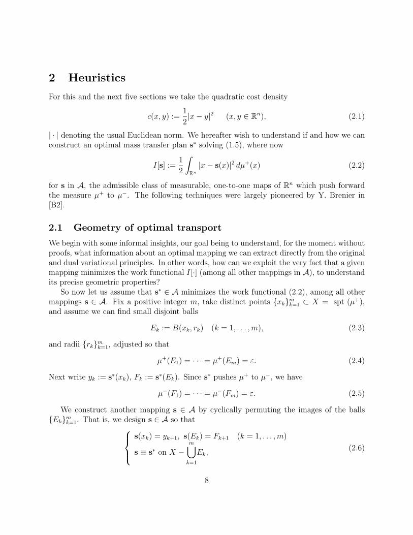
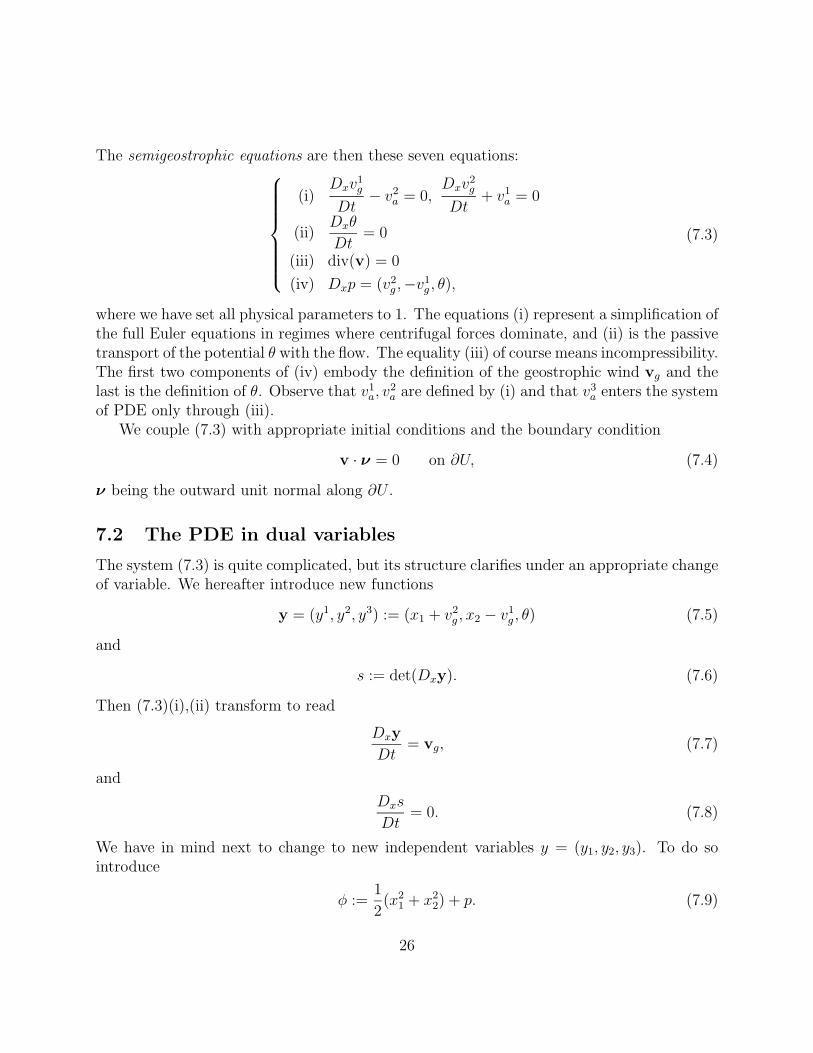
Now let Y (t) denote the range of Dxφ : X → R3, at time t. Then we can in summary

rewrite (7.13), (7.14) to read

(i) rt + div(rw) = 0

(ii) w = (ψy2 − y2,−(ψy1 − y1), 0) in Y (t)× [0,∞)

(iii) det(D2ψ) = r,

(7.16)

27

where we have set w := vg. The additional requirement is

Dψ ∈ X. (7.17)

The system (7.16) is a sort of time-dependent Monge–Ampere equation involving themoving free boundary ∂Y (t). Perhaps more interestingly, (7.16) is an obvious variant of thevorticity formulation of the two-dimensional Euler equations

(i) ωt + div(ωv) = 0

(ii) v = (−ψx2 , ψx1) in R2 × [0,∞).

(iii) ∆ψ = ω,

(7.18)

where ψ is the stream function, and ω the scalar vorticity. Roughly speaking, the system(7.18) is a linearization of (7.16).

F. Otto [O2] and Benamou–Brenier [Be-B1] have shown the existence of a weak solution of(7.16), making use of the pair (φ, ψ) in the sense of the Monge–Kantorovich theory discussedabove. One interpretation is that while r,w evolve on an “order-one” time scale, there is anoptimal Monge–Kantorovich rearrangement of air parcels on a “fast” time scale. See alsoBrenier [B4].

7.3 Frontogenesis

We can informally interpret the dynamics (7.16) as supporting the onset of “fronts”, i.e.surfaces of discontinuity in the velocity and temperature.

To understand this, suppose X, Y (0) are uniformly convex, and for simplicity take r ≡ 1.Then (7.16)(i) is trivial and we can understand (7.16)(ii), (iii) as a law of evolution of ∂Y (t).Suppose for heuristic purposes that ∂Y (t) remains smooth. Then owing to the regularitytheory (§4) ψ(·, t) will be smooth for each t ≥ 0. But since Y (t) is changing shape, it ispresumably possible that Y (t) is no longer convex at some sufficiently large time t.

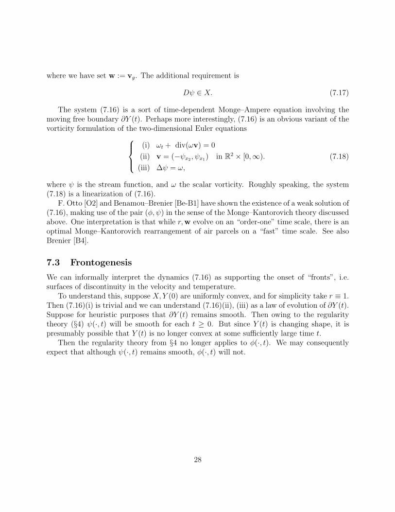
Then the regularity theory from §4 no longer applies to φ(·, t). We may consequentlyexpect that although ψ(·, t) remains smooth, φ(·, t) will not.

28

y=Dφ(x)

x=Dψ(y)

X

Y(t)

Far from being a defect, the advent of singularities of φ(·, t) in the physical variablesx = (x1, x2, x3) is a definite advantage in the model. As discussed in Cullen [C], the me-teorologists wish to model how fronts arise in large scale weather patterns. Tracking thesefronts, that is, thin regions across which there are large variations in wind and tempera-ture, is a central goal, and the semigeostrophic equations provide a plausible mechanismfor frontogenesis. An interesting physical rationale occurs in [C], where the author pointsout that such discontinuities are contact discontinuities in the sense of fluid mechanics: thismeans that the air parcels move parallel to, and not across, them. Obviously in regionsof rapid temperature and wind change the approximations which transform the full Eulerequations into the semigeostrophic PDE are very suspect. But, since the proposed frontsare contact discontinuities, most of the air mass stays away from such regions, and so thevarious approximations should overall be pretty good.

There are extremely interesting mathematical problems here, which have only in smallpart been studied. There are likewise many issues concerning computing these flows: seeBenamou [Be1],[Be2] and Benamou–Brenier [Be-B2] for this.

Part II: Cost = Distance

8 Heuristics

For the rest of this paper we turn attention to the nonuniformly convex cost density

c(x, y) = |x− y| (x, y ∈ Rn). (8.1)

The task now is to find an optimal mass transfer plan s∗ solving Monge’s original problem(1.5), where

I[s] :=

∫Rn

|x− s(x)| dµ+(x) (8.2)

29

for s ∈ A, the admissible class of measurable, one-to-one maps of Rn which push µ+ to µ−.It will turn out that the nonuniform convexity of the cost density (8.1) defeats any simple

attempt to modify the techniques described before in §2–7. We will therefore first of all needsome new insights, to help us sort out the structure of optimal mass allocations.

8.1 Geometry of optimal transport

As in §2 we start with heuristics, our intention being to read off useful information from a“twist variation”.

So assume that s∗ ∈ A minimizes (8.2). Fix then m ≥ 2, select any points {xk}mk=1 ⊂X = spt (µ+), and small balls Ek := B(xk, rk), the radii selected so that µ+(E1) = · · · =µ+(Em) = ε. Next set yk = s∗(xk), Fk := s∗(Ek), and finally fix an integer l ≥ 1. Similarlynow to the construction in §2, we build s ∈ A so that

s(xk) = yk+l, s(Ek) = Fk+l

s ≡ s∗ on X −m⋃

k=1

Ek,

where we compute the subscripts mod m. As in §2 we deduce from the inequality I[s∗] ≤ I[s]that

m∑k=1

|xk − yk| ≤m∑

k=1

|xk − yk+l|. (8.3)

We as follows draw a geometric deduction from (8.3). Take any closed curve C lying inX = spt (µ+), with constant speed parameterization {r(t) | 0 ≤ t ≤ 1}, r(0) = r(1). Letxk := r

(km

)be m equally spaced points along C.

Fix τ > 0. Then using (8.3) and letting m→∞, lm→ τ , we deduce:∫ 1

0

|r(t)− s∗(r(t))|dt ≤∫ 1

0

|r(t)− s∗(r(t + τ))|dt

=

∫ 1

0

|r(t− τ)− s∗(r(t))|dt =: i(τ).

Hence i(·) has a minimum at τ = 0, and so

0 = i′(0) = −∫ 1

0

[r(t)− s∗(r(t))] · r′(t)|r(t)− s∗(r(t))| dt.

This is to say, ∫C

ξ · dr = 0, (8.4)

30

for the vector field

ξ(x) :=s∗(x)− x

|s∗(x)− x| .

As (8.4) holds for all closed curves C, we conclude that ξ is a gradient:

s∗(x)− x

|s∗(x)− x| = −Du∗(x) (8.5)

for some scalar mapping u∗ : Rn → R, which solves the eikonal equation

|Du∗| = 1 (8.6)

on X = spt(µ+). In other words, the direction s∗ maps each point x is given by the gradientof a potential:

s∗(x) = x− d∗(x)Du∗(x).

Note very carefully however that this deduction provides absolutely no information aboutthe distance d∗(x) := |s∗(x)− x|.

Remark. The foregoing insights were first discovered by Monge, based upon completelydifferent, geometric arguments concerning developable surfaces. See Monge [M], Dupin [D].Monge’s and his students’ investigations of this problem lead to many of their foundationaldiscoveries in differential geometry: see for instance Struik [St]. ✷

8.2 Lagrange multipliers

It is interesting to see also a formal, analytic derivation of (8.5), (8.6). The following com-putations are essentially those of Appell [A], from the turn of the century.

We assume for this that dµ+ = f+dx, dµ− = f−dy for smooth densities f±. Theaugmented work functional is

I[s] :=

∫Rr

|x− s(x)|f+(x) + λ(x)[f−(s(x))det(Ds(x))− f+(x)] dx,

where λ is the Lagrange multiplier for the constraint f+ = f−(s)det(Ds). The first variationis

(λf−(s∗)(cofDs∗)ki )xi

=s∗k − xk

|s∗ − x| f+(x) + λf−yk

(s∗)detDs∗.

Simplifying as in §2, we deduce

λxj =s∗k − xk

|s∗ − x| s∗kxj

(j = 1, . . . , n).

31

Next define u∗ byu∗(s∗(x)) = −λ(x).

Then

u∗yks∗kxj

= −λxj =s∗k − xk

|s∗ − x| s∗kxj

.

As Ds∗ is invertible, we see

Du∗(s∗(x)) = − s∗ − x

|s∗ − x| .

But Du∗(s∗(x)) = Du∗(x), and so (8.5), (8.6) again follow.

Remark. It is instructive to compare and contrast the heuristics of this section withthose in §2. The argument based upon the “twist variation” in §8.1 is more general thanthat using cyclic monotonicity in §2.1, and adapts without trouble to a general cost densityc(x, y). The conclusion is then that

Dxc(x, s∗(x)) = Du∗(x) for some scalar potential function u∗. (8.7)

Now if we can invert (8.7), to solve for s∗ in terms of Du∗, we thereby derive a structuralformula for an optimal mapping. Much of the interest in (8.1) is precisely that this inversionis not possible if c is not uniformly convex. ✷

9 Optimal mass transport

9.1 Solution of dual problem

Our intention now is to transform the foregoing heuristic calculations into a proof of theexistence of an optimal mapping s∗, where we expect

s∗(x) = x− d∗(x)Du∗(x) (9.1)

for some potential u∗, with |Du∗(x)| = 1 and so d∗(x) = |s∗(x)− x|.We turn to the case

dµ+ = f+dx, dµ− = f−dy (9.2)

where f± are bounded, nonnegative functions with compact support, satisfying the massbalance compatibility condition ∫

X

f+(x) dx =

∫Y

f−(y) dy (9.3)

where X = spt(f+), Y = spt(f−).

32

We further remember the dual problem (§1), which asks us to find (u∗, v∗) to maximize

K[u, v] :=

∫X

u(x)f+(x) dx +

∫Y

v(y)f−(y) dy (9.4)

subject to

u(x) + v(y) ≤ |x− y| (x ∈ X, y ∈ Y ). (9.5)

Lemma 9.1 (i) There exist (u∗, v∗) solving this maximization problem.(ii) Furthermore, we can take

v∗ = −u∗, (9.6)

where u∗ : Rn → R is Lipschitz continuous, with

|u∗(x)− u∗(y)| ≤ |x− y| (x, y ∈ Rn). (9.7)

Proof. 1. If u, v satisfy (9.5), then

u(x) ≤ infy∈Y

(|x− y| − v(y)) =: u(x) (9.8)

andu(x) + v(y) ≤ |x− y| (x ∈ X, y ∈ Y ).

Therefore

v(y) ≤ minx∈X

(|x− y| − u(x)) =: v(y) (9.9)

and

u(x) + v(y) ≤ |x− y| (x ∈ X, y ∈ Y ). (9.10)

Furthermore, since v ≥ v, (9.8) implies

u(x) ≥ miny∈Y

(|x− y| − v(y));

and so (9.10) implies

u(x) = miny∈Y

(|x− y| − v(y)). (9.11)

Since f± ≥ 0 and u ≥ u, v ≥ v we see that K[u, v] ≤ K[u, v].

33

2. Thus in seeking to maximize K we may restrict attention to “dual” pairs (u, v), asabove. But then

u + v = 0 on X ∩ Y. (9.12)

To see this, take z ∈ X ∩ Y (if X ∩ Y �= ∅), and suppose

u(z) + v(z) < 0. (9.13)

Take x ∈ X, y ∈ Y so that {u(z) = |z − y| − v(y)

v(z) = |x− z| − u(x).

Rearrange and add:

|x− z|+ |z − y| = u(x) + v(y) + u(z) + v(z)

< u(x) + v(y) by (9.13)

≤ |x− y| by (9.10).

This contradiction shows u + v ≥ 0 on X ∩Y . As (9.10) clearly implies u + v ≤ 0 on X ∩Y ,assertion (9.12) follows.

3. In view of (9.12) let us extend the definition of u by setting

u := −v on Y.

Then (9.10) readsu(x)− u(y) ≤ |x− y| (x ∈ X, y ∈ Y ).

Finally it is an exercise to check that we can extend u to all of Rn, so that

|u(x)− u(y)| ≤ |x− y| (x, y ∈ Rn).

Our problem is thus to maximize

K[u] :=

∫Rn

u(f+ − f−) dz, (9.14)

subject to the Lipschitz constraint

|u(x)− u(y)| ≤ |x− y| (x, y ∈ Rn). (9.15)

This problem clearly admits a solution u∗, and we define v∗ := −u∗ to obtain a pair solvingthe original dual problem. ✷

Note that the Lipschitz condition implies that Du∗ exists a.e. in Rn, with

|Du∗| ≤ 1 a.e. .

We further expect|Du∗| = 1 a.e. on X ∪ Y.

34

9.2 Existence of optimal mass transfer plan

We wish next to employ u∗ to build an optimal mass allocation mapping s∗. This is not soeasy as in the uniformly convex case that c(x, y) = 1

2|x − y|2, discussed in §3. The central

problem is that although we expect s∗ to have the structure (9.1) there is still an unknown,namely the distance d∗(x) = |s∗(x)− x| that the point x should move: Du∗(x) tells us onlythe direction.

This problem was solved by Sudakov [Su] using rather subtle measure theoretic techniques(but see also the comments in Ambrosio [Am].). In keeping with the overall theme of thispaper, we will here discuss instead an alternative, differential-equations-based procedure,from [E-G1]. Our argument introduces some useful ideas, but is really complicated. Farbetter proofs have been recently found by Trudinger–Wang [T-W] and [C-F-M] Caffarelli–Feldman–McCann.

To repeat, the basic issue is that we must somehow extract the missing information aboutthe distance d∗(x) = |s∗(x)− x| from the variational problem (9.14), (9.15). It is convenientin doing so to introduce some standard notion from convex analysis. Let us set

K := {u ∈ L2(Rn) | |Du| ≤ 1 a.e.} (9.16)

and

I∞[u] :=

{0 if u ∈ K+∞ otherwise.

(9.17)

Then u∗ minimizes K[·] over K. The corresponding Euler Lagrange equation is

f+ − f− ∈ ∂I∞[u∗]; (9.18)

that is,I∞[v] ≥ I∞[u∗] + (f+ − f−, v − u∗)L2

for all v ∈ L2(Rn).We need firstly to convert (9.18) into more concrete form:

Lemma 9.2 Assume additionally that f± are Lipschitz continuous.(i) Then there exists a nonnegative L∞ function a such that

− div(aDu∗) = f+ − f− in Rn. (9.19)

(ii) Furthermore|Du| = 1 a.e. on the set {a > 0}.

35

We call a the transport density. The PDE (9.19) looks linear, but is not: the function a isthe Lagrange multiplier corresponding to the constraint |Du∗| ≤ 1, and is a highly nonlinearand nonlocal function of u∗. On the other hand once u∗ is known, (9.19) can be thought ofas a linear, first-order PDE for a.

Outline of Proof. Take n + 1 ≤ p <∞. We approximate by the quasilinear PDE

− div(|Dup|p−2Dup) = f+ − f−, (9.20)

which corresponds to the problem of maximizing

Kp[u] :=

∫Rn

u(f+ − f−)− 1

p|Du|p dz.

A maximum principle argument shows that

supp|up|, |Dup|, |Dup|p ≤ C <∞

for some constant C. (Cf. Bhattacharya–DiBenedetto–Manfredi [B-B-M].)It follows that there exists a sequence pk →∞ such that

upk→ u∗ locally uniformity

Dupk→ Du∗ boundedly, a.e.

|Dupk|p−2 ⇀ a weakly ∗ in L∞.

Then passing to limits in (9.20) we obtain (9.19). ✷

As noted above, a is the Lagrange multiplier from the constraint |Du∗| ≤ 1. It turns outfurthermore that a in fact “contains” the missing information as to the distance d∗(x).

The recipe is to build s∗ by solving a flow problem involving Du∗, a, etc. So fix x ∈ Xand consider the ODE {

z(t) = b(z(t), t) (0 ≤ t ≤ 1)

z(0) = x,(9.21)

for the time-varying vector field

b(z, t) :=−a(z)Du∗(z)

tf−(z) + (1− t)f+(z). (9.22)

Ignore for the moment that a, Du∗ are not smooth (or even continuous in general) and thatwe may be dividing by zero in (9.22). Proceeding formally then, let us write

s∗(x) = z(1), (9.23)

the time-one map of the flow.

36

Theorem 9.1 Define s∗ by (9.23). Then(i) s∗ : X → Y is essentially one-to-one and onto.(ii)

∫X

h(s∗(x)) dµ+(x) =∫

Yh(y) dµ−(y) for each h ∈ C(Y ).

(iii) Lastly, ∫X

|x− s∗(x)| dµ+(x) ≤∫

X

|x− s(x)| dµ+(x)

for all s : X → Y such that s#(µ+) = µ−.

Outline of Proof. 1. Write

s(t, x) := z(t) (0 ≤ t ≤ 1),

J(z, t) := detDs(z, t).

Then Jt = (div b)J ; and so, following Dacorogna–Moser [D-M], we may compute

∂

∂t[(tf−(s(z, t)) + (1− t)f+(s(z, t)))J(z, t)]

= (f− − f+)J + (tDf− · st + (1− t)Df+ · st)J

+(tf− + (1− t)f+)Jt

= [(f− − f+) + (tDf− · b + (1− t)Df+ · b)

+(tf− + (1− t)f+)div b]J.

(9.24)

But in view of (9.19), (9.22):

div b =f+ − f−

tf− + (1− t)f++

(tDf− + (1− t)Df+) · (aDu∗)

(tf− + (1− t)f+)2

=f+ − f− − (tDf− + (1− t)Df+) · b

tf− + (1− t)f+.

Consequently the last term in (9.24) is zero, and hence

f−(s∗)detDs∗ = f+.

This confirms assertion (ii).2. We next verify s∗ is optimal. For this, take s to be any admissible mapping.

37

Then ∫X

|x− s∗(x)| dµ+(x) =

∫X

[u∗(x)− u∗(s∗(x))]f+(x) dx

=

∫X

u∗f+ −∫

Y

u∗f− dy

=

∫X

[u∗(x)− u∗(s(x))]f+(x) dx

≤∫

X

|x− s(x)|f+(x) dx.

✷

This “Theorem” should of course really be in quotes, since the “proof” just outlined ispurely formal. In reality neither a nor Du∗ nor f± are smooth enough to justify these com-putations. A careful proof is available in [E-G1]: the full details are extremely complicated,involving a very careful smoothing of u∗. The proof requires as well the additional conditionsthat ∂X, ∂Y are nice and X ∩Y = ∅, although these requirements are presumably not reallynecessary.

Remark. A nice paper by Cellina and Perrotta [C-P] discusses somewhat related issues.Jensen [Je] considers the subtle problem of what happens to the approximations up withinthe regions {f+ ≡ f− ≡ 0}, in the limit p→∞.

More on the connections with optimal flow problems may be found in Iri [I] and Strang[S1], [S2]. ✷

9.3 Detailed mass balance, transport density

For reference later we record here some properties of the optimal potential u∗ and transportdensity a, proved in [E-G1].

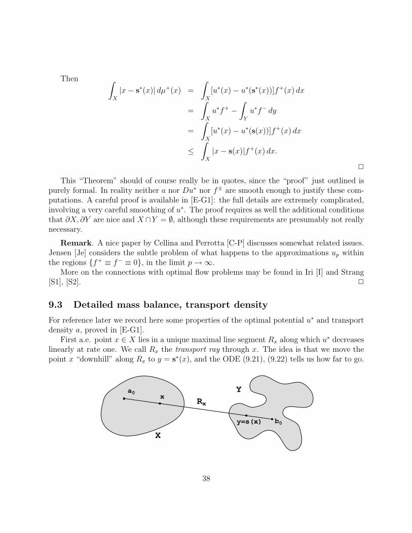
First a.e. point x ∈ X lies in a unique maximal line segment Rx along which u∗ decreaseslinearly at rate one. We call Rx the transport ray through x. The idea is that we move thepoint x “downhill” along Rx to y = s∗(x), and the ODE (9.21), (9.22) tells us how far to go.

X

Ya0

b0

x

y=s(x)

Rx

38

Next we note that these transport rays subdivide X and Y into subregions of equal µ+, µ−

measure.

Lemma 9.3 Let E ⊂ Rn be a measurable set with the property that for each point x ∈ E,the full transport ray Rx also lies in E. Then∫

X∩E

f+ dx =

∫Y ∩E

f− dy. (9.25)

We call (9.25) the detailed mass balance relation. It asserts that the line segments alongwhich u∗ changes linearly with slope one naturally partition X and Y into subregions ofequal masses. This must be so if our transport scheme (9.23) is to work.

Outline of Proof. We provide an interesting, but purely heuristic, derivation of a somewhatweaker statement. The trick is to employ a Hamilton–Jacobi PDE to generate a variationfor the maximization principle (9.14), (9.15).

For this, take H : Rn → R to be any smooth Hamiltonian. We solve then the initial-valueproblem: {

wt + H(Dw) = 0 in Rn × {t > 0}w = u∗ on Rn × {t = 0}. (9.26)

Now the mapping t → w(·, t) is a contraction in the sup-norm, and therefore for each timet > 0:

‖Dw(·, t)‖L∞ ≤ ‖Du∗(·, t)‖L∞ ≤ 1.

Hence w(·, t) is a valid competitor in the variational principle. Since u∗ solves (9.14), (9.15)and w(·, 0) = u∗, it follows that

i(t) ≤ i(0) (t ≥ 0),

where

i(t) :=

∫Rn

w(·, t)(f+ − f−)dz.

Hence i′(0) ≤ 0. In view of (9.26) therefore,∫Rn

H(Du∗)(f+ − f−)dz = −i′(0) ≥ 0.

Replacing H by −H, we conclude that∫Rn

H(Du∗)(f+ − f−)dz = 0 (9.27)

39

for all smooth H : Rn → R.Taking H to approximate χA, where A ⊂ Sn−1, we deduce from (9.27) that the detailed

mass balance holds for the particular set E := {z | Du∗(z) ∈ A}. ✷

This proof is not really rigorous as u∗, w are not smooth enough to justify the statedcomputations. See e.g. [E-G1] for a careful proof.

It is also useful to understand how smooth the transport density is along the transportrays, and we also need to check that the ODE flow (9.21) does not “overshoot” the endpoints.

Lemma 9.4 (i) For a.e. x, the transport density a, restricted to Rx, is locally Lipschitzcontinuous.

(ii) Furthermore,lim

z→a0,b0z∈Rx

a(z) = 0,

where a0, b0 are the endpoints of Rx.

The first calculations in the literature related to assertion (ii) seem to be those of Janfalk[J].

Remark. The argument discussed above introduces various ideas useful in the followingapplications, but is very complicated in detail. Far superior, and much shorter, proofshave been independently found by Trudinger–Wang [T-W] and [C-F-M] Caffarelli–Feldman–McCann. A clear proof is also available in Ambrosio [Am]. ✷

10 Application: Shape optimization

The ensuing three sections describe some applications extending the ideas set forth in §8,9.As a first application, we discuss the following shape optimization problem. Suppose we

are given two nonnegative Radon measures µ± on Rn, with µ+(Rn) = µ−(Rn). Think of µ+

as giving the density of a given electric charge. We interpret Rn as an insulating medium,into which we place a fixed amount of some conducting material, whose conductivity (=inverse resistivity) is described by a nonnegative measure σ. We imagine then the resultingsteady current flow within Rn from µ+ to µ−, and ask if we can optimize the placement ofthe conducting material so as to minimize the heating induced by the flow.

To be more precise, consider the admissible class

S = {nonnegative Radon measures σ on Rn | σ(Rn) = 1}

and think of each σ ∈ S as describing how to arrange a unit quantity of conducting materialwithin Rn. Corresponding to each σ ∈ S and scalar function v ∈ C∞c (Rn) we define

E(σ, v) :=1

2

∫Rn

|Dv|2 dσ −∫Rn

v d(µ+ − µ−). (10.1)

40

Then

E(σ) := inf{E(σ, v) | v ∈ C∞c (Rn)} (10.2)

represents the negative of the Joule heating (= energy dissipation) corresponding to thegiven conductivity. If there exists v ∈ C∞c (Rn) giving the minimum, then

− div(σDv) = µ+ − µ− in Rn; (10.3)

that is, ∫Rn

Dv ·Dw dσ =

∫Rn

w d(µ+ − µ−)

for each w ∈ C∞c (Rn). We can interpret{v = electrostatic potential, e = −Dv = electric field,j = σe = current density (by Ohm’s law).

We now ask: Can we find σ∗ ∈ S to maximize E(σ)? In other words, is there an optimalway to arrange the given amount of conductivity material so as to minimize the heating?

Following Bouchitte–Buttazzo–Seppechere [B-B-S], we introduce the related Monge–Kan-torovich dual problem of maximizing ∫

Rn

u d(µ+ − µ−) (10.4)

among all u : Rn → R, with

|u(x)− u(y)| ≤ 1 (x, y ∈ Rn). (10.5)

Lemma 10.1 (i) There exists u∗ solving (10.4), (10.5).(ii) Furthermore, there exists α∗ ∈ A such that{

−div(α∗Du∗) = µ+ − µ−

|Du∗| = 1 α∗ a.e.(10.6)

This is clearly a generalization of our work in §9. Note carefully that since α∗ is merelya Radon measure, and thus may be in part singular with respect to n-dimensional Lebesguemeasure, care is needed in interpreting the PDE in (10.6): see [B-B-S].

Now set {σ∗ := (α∗(Rn))−1α∗

v∗ := α∗(Rn)u∗(10.7)

41

Then σ∗ ∈ S and

− div(σ∗Dv∗) = µ+ − µ− in Rn. (10.8)

We claim now that

E(σ∗) = maxσ∈S

E(σ). (10.9)

For this we invoke another duality principle, namely

E(σ) = sup

{−1

2

∫Rn

|e|2 dσ | div(σe) = µ+ − µ−}

. (10.10)

Now if u satisfies (10.5) and div(σe) = µ+ − µ−, then∫Rn

u d(µ+ − µ−) = −∫Rn

Du · e dσ

≤(∫

Rn

|Du|2 dσ

)1/2 (∫Rn

|e|2 dσ

)1/2

≤(∫

Rn

|e|2 dσ

)1/2

,

since |Du| ≤ 1 and σ(Rn) = 1. Taking the suprema over all u, we deduce

−1

2

∫Rn

|e|2 dσ ≤ −1

2α∗(Rn)2.

In light of (10.10), then

E(σ) ≤ −1

2α∗(Rn). (10.11)

But since |Du∗| = 1 σ∗ a.e., we compute for e∗ := −Dv∗ that

E(σ∗) ≥ −1

2

∫Rn

|e∗|2 dσ∗ = −1

2α∗(Rn)2.

According then to (10.11), σ∗ is optimal.

Remark. Results strongly related to these are to be found in earlier work of Iri [I] andStrang [S1], [S2]. ✷

42

11 Application: Sandpile models

As a completely different class of applications, we next introduce some physical “sandpile”models evolving in time, for which we can identify a Monge–Kantorovich mass transfermechanism on a “fast” time scale. In the following examples we regard u as the heightfunction of our sandpiles: the constraint

|Du| ≤ 1 (11.1)

is everywhere imposed, and has the physical meaning that the sand cannot remain in equilib-rium if the slope anywhere exceeds the angle of repose π/4. We will later reinterpret (11.1)as the Monge–Kantorovich constraint: the interplay of these interpretations animates muchof the following. The exposition is based in part upon the interesting papers of Prigozhin[P1], [P2], [P3], and also upon [E-F-G], [A-E-W], [E-R].

11.1 Growing sandpiles

As a simple preliminary model, suppose that the function f ≥ 0 is a source term, representingthe rate that sand is added to a sandpile, whose initial height is zero. We then have ut = fin any region where the constraint (11.1) is active. But if adding more sand at some locationwould break the constraint, we may imagine the newly added sand particles “to roll downhillinstantly”, coming to rest at new sites where their addition maintains the constraint.

We propose as a model for the resulting evolution:{f − ut ∈ ∂I∞[u] (t > 0)

u = 0 (t = 0),(11.2)

the functional I∞[·] defined in §9. The interpretation is that at each moment of time, themass dµ+ = f+(·, t)dx is instantly and optimally transported downhill by the potential u(·, t)into the mass dµ− = ut(·, t)dy. In other words the height function u(·, t) of the sandpile isdeemed also to be the potential generating the Monge–Kantorovich reallocation of f+dx toutdy. This requirement forces the dynamics (11.2).

Example: Interacting sandcones. Consider, for example, the case that mass is addedonly at fixed sites:

f =m∑

k=1

fk(t)δdk, (11.3)

where fk > 0. In this case we expect the height function u to be the union of interactingsandcones:

u(x, t) = max{0, z1(t)− |x− d1|, . . . , zm(t)− |x− dm|}. (11.4)

43

Owing to conservation of mass, we expect the cone heights z(t) = (z1(t), . . . , zm(t)) to solvethe coupled system of ODE

zk(t) =fk(t)

|Dk(t)|(t ≥ 0)

zk(0) = 0

(11.5)

for k = 1, . . . , m, where |Dk(t)| denotes the measure of the set Dk(t) ⊂ Rn on which the k-thcone determines u:

Dk(t) = {x ∈ Rn | zk(t)− |x− dk| > 0, zl(t)− |x− dl| for l �= k}. (11.6)

These ODE were originally derived by Aronsson [AR1].Let us confirm that (11.4)–(11.6) give the solution of (11.2), in the case of point sources

(11.3). To check (11.2) we must show at each time t ≥ 0 that

I∞[u] + (f − ut, v − u)L2 ≤ I∞[v] (11.7)

for all v ∈ L2(Rn). Now I∞[u(·, t)] = 0, and if I∞[v] = +∞, then (11.7) is obvious. So wemay as well assume I∞[v] = 0; that is,

|Dv| ≤ 1 a.e. (11.8)

The problem now is to show that

(f − ut(·, t), v − u(·, t))L2 ≤ 0. (11.9)

Owing to (11.3) and (11.4), the term on the left means

m∑k=1

fk(t)(v(dk)− u(dk, t))−∞∑

k=1

∫Dk(t)

zk(t)(v(x)− u(x, t)) dx.

Consequently the ODE (11.5) means that we must show

m∑k=1

fk(t)

∫−

Dk(t)

v(dk)− v(x) dx ≤m∑

k=1

fk(t)

∫−

Dk(t)

u(dk, t)− u(x, t) dx,(11.10)

the slash through the integral signs denoting average. But (11.10) is easy: in light of (11.8)and (11.4), we have

v(dk)− v(x) ≤ |dk − x| = u(dk, t)− u(x, t)

on Dk(t). ✷

44

11.2 Collapsing sandpiles

The dynamics (11.2) model “surface flows” for sandpiles: once a sand grain is added, rollsdownhill and comes to rest, it never again moves. It is therefore interesting to modify thismodel to allow for “avalanches”.

In view of the approximation in §9 of the term ∂I∞[u] by the p-Laplacian operator−div(|Du|p−2Du), we propose now to investigate the limiting behavior as p → ∞ of thequasilinear parabolic problem{

up,t − div(|Dup|p−2Dup) = 0 in Rn × (0,∞)

up = g on Rn × {t = 0}. (11.11)

Here g : Rn → R is the given initial height of a sandpile, satisfying the instability condition

L := supRn

|Dg| > 1. (11.12)

For large p, the PDE in (11.11) supports very fast diffusion in regions where |Dup| > 1 andvery slow diffusion in regions where |Dup| < 1. We expect therefore that for p >> 1 thesolutions up of (11.11) will rapidly rearrange its mass to achieve the stability condition. Asthe initial profile is unstable, we expect there to be a short time period during which thereis rapid mass flow, followed by a time in which up is practically unchanging.

Indeed, simple estimates suffice to show that there exists a function u = u(x) with

|Du| ≤ 1 in Rn (11.13)

such that

upk→ u uniformly on compact subsets of Rn × (0,∞) (11.14)

for some sequence pk →∞. We call u the collapsed profile and our problem is to understandhow the initial, unstable profile g rearranges itself into u.

To understand the mapping g �→ u, we rescale the PDE (11.11) to stretch out the initialtime layer of rapid mass motion. For this, set

vp(x, t) := tup

(x,

tp−1

p− 1

)(x ∈ Rn, t > 0) (11.15)

and write τ := L−1. It turns out then that

vpk→ v uniformly on Rn × [τ, 1],

where { v

t− vt ∈ ∂I∞[v] (τ ≤ t ≤ 1)

v = h (t = τ)(11.16)

45

for h := 1Lg. Furthermore the collapsed profile is

u = v(·, 1). (11.17)

In summary, our procedure for calculating the collapse g �→ u is to define h as above, solvethe evolution (11.16) and then set u := v(·, 1).

Now (11.16) is interpreted, as above, as an evolution in which the mass dµ+ = vtdx is

instantly and optimally rearranged by the potential v into dµ− = vtdy. Again we have aMonge–Kantorovich mass reallocation occurring on a fast time scale, which thereby generatesthe dynamics (11.16).

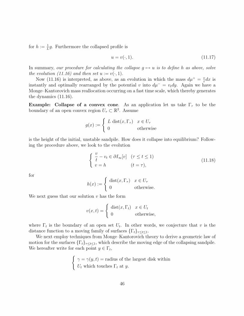
Example: Collapse of a convex cone. As an application let us take Γτ to be theboundary of an open convex region Uτ ⊂ R2. Assume

g(x) :=

{L dist(x, Γτ ) x ∈ Uτ

0 otherwise

is the height of the initial, unstable sandpile. How does it collapse into equilibrium? Follow-ing the procedure above, we look to the evolution{ v

t− vt ∈ ∂I∞[v] (τ ≤ t ≤ 1)

v = h (t = τ),(11.18)

for

h(x) :=

{dist(x, Γτ ) x ∈ Uτ

0 otherwise.

We next guess that our solution v has the form

v(x, t) =

{dist(x, Γt) x ∈ Ut

0 otherwise,

where Γt is the boundary of an open set Ut. In other words, we conjecture that v is thedistance function to a moving family of surfaces {Γt}τ≤t≤1.

We next employ techniques from Monge–Kantorovich theory to derive a geometric law ofmotion for the surfaces {Γt}τ≤t≤1, which describe the moving edge of the collapsing sandpile.We hereafter write for each point y ∈ Γt,{

γ = γ(y, t) = radius of the largest disk within

Ut which touches Γt at y.

46

Take a point x ∈ Ut with a unique closest point y ∈ Γt. Let κ := curvature of Γt at y andR := 1

κ.

We may assume the segment [x, y] is vertical and y = (0, R). Set

Aε := {z | θ(z, e2) < ε, R− γ ≤ |z| ≤ R},

where θ(z, e2) denotes the angle between z and e2 = (0, 1). Now we interpret (11.18) assaying that the mass dµ+ = v

tdx is transferred in the direction −Dv, to dµ− = vtdy. This

transfer, restricted to the set Aε, forces the (approximate) detailed mass balance relation∫Aε

v

tdx ≈

∫Aε

vt dy, (11.19)

according to Lemma 9.3. Now divide both sides by |Aε| and send ε → 0. A calculationshows

limε→0

∫−

Aε

v

tdx =

γ

3t

(3− 2κγ

2− κγ

)

and, since vt = V (= outward normal velocity of Γt at y) along the ray through y,

limε→0

∫−

Aε

vt dy = V.

We derive therefore the nonlocal geometric law of motion

V =γ

3t

(3− 2κγ

2− κγ

)on Γt (11.20)

for the moving surfaces {Γt}τ≤t≤1. (See Feldman [F] for a rigorous analysis of (11.20).)

11.3 A stochastic model

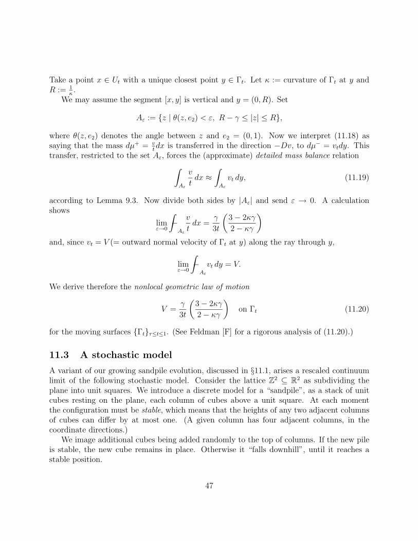
A variant of our growing sandpile evolution, discussed in §11.1, arises a rescaled continuumlimit of the following stochastic model. Consider the lattice Z2 ⊆ R2 as subdividing theplane into unit squares. We introduce a discrete model for a “sandpile”, as a stack of unitcubes resting on the plane, each column of cubes above a unit square. At each momentthe configuration must be stable, which means that the heights of any two adjacent columnsof cubes can differ by at most one. (A given column has four adjacent columns, in thecoordinate directions.)

We image additional cubes being added randomly to the top of columns. If the new pileis stable, the new cube remains in place. Otherwise it “falls downhill”, until it reaches astable position.

47

What happens in the scaled continuum limit, when we take more and more, smaller andsmaller cubes added faster and faster?

AAAA

AAAA

AA

AAAA

AA

AAAA

We make precise our model, generalizing to Rn. Let us write i = (i1, . . . , in) for a typicalsite in Zn and say two sites i, j are adjacent, written i ∼ j, if

max1≤k≤n

|ik − jk| = 1.

A (stable) configuration is a mapping η : Zn → Z such that{|η(i)− η(j)| ≤ 1 if i ∼ j

and η has bounded support.

The state space S is the collection of all configurations.We introduce as follows a Markov process on S. Given η ∈ S and i ∈ Zn, write

Γ(i, η) := {j ∈ Zn | there exist sites i = i1 ∼ i2 ∼ · · · ∼ im = j

with η(il+1) = η(il)− 1 (l = 1, . . . , m− 1),

η(k) �= η(j)− 1 for all k ∼ j}. (11.21)

Thus Γ(i, η) is the set of sites j at which a cube newly added to i can come to rest. Assignto each j ∈ Γ(i, η) a number

0 ≤ p(i, j, η) ≤ 1

such that ∑j∈Γ(i,η)

p(i, j, η) = 1, (11.22)

and think of p(i, j, η) as the probability that a cube added to i will fall downhill and cometo rest at j. Finally set

c(j, η, t) :=∑

i:j∈Γ(i,η)

p(i, j, η)f

(i

N,

t

N

)(11.23)

48

where f : Rn × [0,∞)→ [0,∞) is a given function, the source density. Then c(j, η, t) is therate at which cubes are coming to rest at j.

We introduce the infinitesimal generator Lt of our Markov process by taking any F :S → R and defining then

(LtF )(η) :=∑j∈Zn

c(j, η, t)(F (ηj)− F (η)), (11.24)

where

ηj(i) :=

{η(i) + 1 if i = j

η(i) if i �= j.

The formula (11.24) encodes the foregoing probabilistic interpretation.Let {η(·, t)}t≥0 denote the inhomogeneous Markov process on S generated by {Lt}t≥0,

with η(·, 0) ≡ 0. Thus η(i, t) is the (random) height of the pile of cubes at site i, time t ≥ 0.We intend now to rescale, taking now cubes of side 1

Nadded on a time scale multiplied

by N . We construct therefore the rescaled process 1N

η([xN ], tN), where x ∈ Rn, t ≥ 0, andinquire what happens as N →∞.

Theorem 11.1 For each t ≥ 0, we have

E

(supx∈Rn

∣∣∣∣ 1

Nη([xN ], tN)− u(x, t)

∣∣∣∣)→ 0 (11.25)

as N →∞, where u is the unique solution of the evolution{f − ut ∈ ∂I[u] (t = 0)

u = 0 (t = 0).(11.26)

Here

I[v] :=

{0 if v ∈ K+∞ otherwise

forK := {v ∈ L2(Rn) | v is Lipschitz, |vxi

| ≤ 1 a.e. (i = 1, . . . , n)}.Consequently, the continuum dynamics (11.26), while similar to (11.2), differ by “remem-bering” the anisotropic structure of the lattice.

The proof in [E-R] is too complicated to reproduce here: the key new idea is a combina-torial lemma asserting that if η, ξ are any two configurations in S, then

∑j

c(j, η, t)(η(j)− ξ(j)) ≤∑

i

f

(i

N,

t

N

)(η(i)− ξ(i)). (11.27)

49

Since the term c, describing the rate at which cubes come to rest at a given site, is a sort ofrescaled, discrete analogue of ut, (11.27) is a “microscopic” analogue of the “macroscopic”inequality ∫

Rn

(f − ut)(v − u)dx ≤ 0 (v ∈ K).

But this is just, as we have seen before, another way of writing the evolution (11.26).A further interpretation of (11.26) is that the mass dµ+ = fdx is instantly rearranged

into dµ− = utdy, so as to minimize the cost∫Rn

c(x, s(x))f+(x) dx

for the l1-distancec(x, y) = |x1 − y1|+ · · ·+ |xn − yn|.

In the case of point sources, f =∑

fk(t)δdk, the dynamics (11.26) correspond to growing,

interacting pyramids of sand.

12 Application: Compression molding

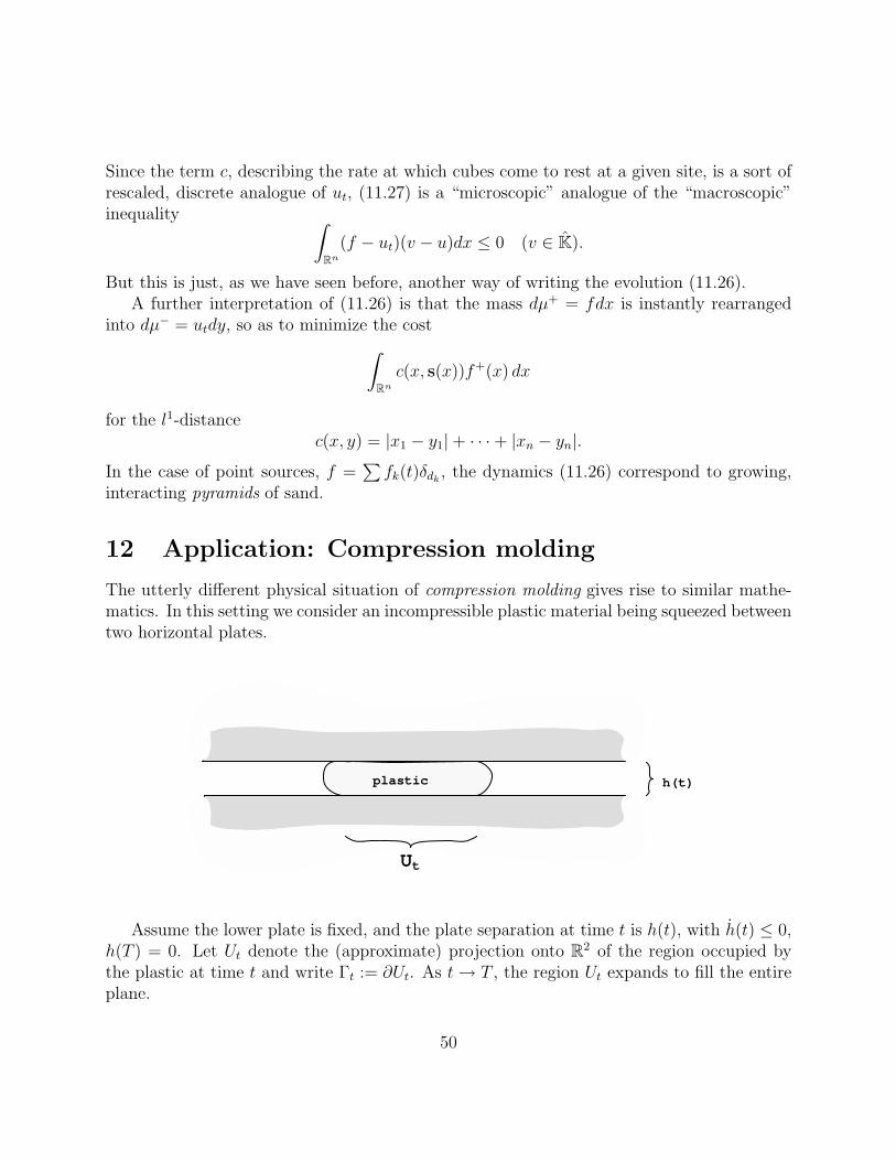
The utterly different physical situation of compression molding gives rise to similar mathe-matics. In this setting we consider an incompressible plastic material being squeezed betweentwo horizontal plates.

plastic

Ut

h(t)

Assume the lower plate is fixed, and the plate separation at time t is h(t), with h(t) ≤ 0,h(T ) = 0. Let Ut denote the (approximate) projection onto R2 of the region occupied bythe plastic at time t and write Γt := ∂Ut. As t→ T , the region Ut expands to fill the entireplane.

50

Following [AR2], [A-E], we introduce a highly simplified model of the physics, with thegoal of tracking the air-plastic interface Γt for times 0 ≤ t < T . After a number of simplifyingassumptions for this highly viscous flow, the relevant PDE becomes

div(|Dp| 1σ−1Dp) =h

hin Ut (12.1)

where 0 ≤ t < T , p = pressure, and σ is a small constant arising in a power-law constitutiverelation for the highly non-Newtonian flow.

We can rescale in time to convert to the case T = ∞, h/h ≡ −1, in which case (12.1)reads

− div(|Dp| 1σ−1Dp) = 1 in Ut (12.2)

for t ≥ 0. In addition, we have the boundary conditions{p = 0 on Γt

V = |Dp|1/σ on Γt,(12.3)

where V = outward normal velocity of Γt.Now experimental results in the engineering literature suggest that for real materials the

evolution of Γt does not much depend upon the exact choice of σ, so long as σ is small: see,for instance, [F-F-T]. We therefore propose to study the asymptotic limit σ → 0. For this,we first change notation, and rewrite (12.2), (12.3) as{

−div(|Dup|p−2Dup) = 1 in Ut

up = 0, V = |Dup|p−2 on Γt.(12.4)

When p→∞, we expect in light of the calculations in §9 that up → u, where{−div(aDu) = 1 in Ut

u = 0, V = a on Γt

(12.5)

for some nonnegative function a. The physical interpretations are now{u = pressure, v = −aDu = velocity,

a = speed.

We can further reinterpret (12.5) as the evolution

w − wt ∈ ∂I∞[u](t > 0)

u ∈ β(w),(12.6)

51

where β is the multivalued mapping

β(x) =

[0,∞) if x ≥ 1

0 if 0 ≤ x ≤ 1

(−∞, 0] if x ≤ 0.

We interpret w = χUt , and so the initial condition for (12.6) is

w = χU0 (t = 0). (12.7)

The Monge–Kantorovich interpretation is that at each moment the measure dµ+ = χUtdxis being instantly and optimally rearranged to dµ− = V times (n-1)-dimensional Hausdorffmeasure Hn−1 restricted to Γt. These dynamics in turn determine the velocity V of Γt.

It is not hard to check that

u(x, t) =

{dist(x, Γt) x ∈ Ut

0 otherwise;

so that the pressure in this asymptotic model is just the distance to the boundary.Using detailed mass balance arguments somewhat like those in §11 we can further show

that

V = γ(1− κγ

2

)on Γt (12.8)

where γ = radius of largest disk within Ut touching Γt at y and κ = curvature. Feldman [F]has rigorously analyzed this geometric flow that characterizes the spread of the plastic.

Appendix

13 Finite-dimensional linear programming

To motivate some functional analytic considerations in §1, we record here some facts aboutlinear programming. Good references are Bertsimas–Tsitsiklis [B-T], Ekeland–Turnbull [E-T]or Papadimitriou–Steiglitz [P-S].

Notation. If x = (x1, . . . , xN) ∈ RN , we write

x ≥ 0

to mean xk ≥ 0 (k = 1, . . . , N). ✷

52

Assume we are given c ∈ RN , b ∈ RM , and an M ×N matrix A.The primal linear programming problem is to find x∗ ∈ RN so as to

(P)

{minimize c · x, subject to the

constraints Ax = b, x ≥ 0.

The dual problem is then to find y∗ ∈ RM so as to

(D)

{maximize b · y, subject to the

constraints AT y ≤ c.

Assume x∗ ∈ RN solves (P), y∗ ∈ RM solves (D). We may then regard y∗ as the Lagrangemultiplier for the constraints in (P), and, likewise, x∗ as the Lagrange multiplier for (D).Furthermore we have the saddle point relation:

c · x∗ = b · y∗; (13.1)

that is,

min{c · x | Ax = b, x ≥ 0} = max{b · y | AT y ≤ c}. (13.2)

An example. Suppose we are given nonnegative numbers cij, µ+i , µ−j (i = 1, . . . , n; j =

1, . . . , m), withn∑

i=1

µ+i =

m∑j=1

µ−j ,

and we are asked to find µ∗ij (i = 1, . . . , n; j = 1, . . . , m), so as to

minimizen∑

i=1

m∑j=1

cijµij, (13.3)

subject to the constraints

m∑j=1

µij = µ+i ,

n∑i=1

µij = µ−j , µij ≥ 0 (i = 1, . . . , n; j = 1, . . . , m). (13.4)

Papadimitriou and Steiglitz call this the Hitchcock problem. It has the form (P), with{N = nm, M = n + m, x = (µ11, µ12, . . . , µ1m, µ21, . . . , µnm),

c = (c11, . . . , c1m, c21, . . . , cnm), b = (µ+1 , . . . , µ+

n , µ−1 , . . . , µ−m),

53

and A the (n + m)× nm matrix

n rows

m rows

11 0 . . . 00 11 . . . 00 0 . . . 11

. . . . . . . . . . . .

e1 e1 . . . e1

e2 e2 . . . e2

em em . . . em

Above the middle horizontal dotted line, each entry is a row vector in Rm and 11 = (1, . . . , 1),0 = (0, 0, . . . , 0). Below the dotted line each entry is a row vector inRn and ei = (0, 0, . . . , 1, . . . , 0),the 1 in the i-th slot (i = 1, . . . , n).

Now write y = (u1, . . . , un, v1, . . . , vm) ∈ Rn+m. Employing the explicit form of the matrixA, we translate the dual problem (D) for the case at hand to read

maximizen∑

i=1

uiµ+i +

m∑j=1

vjµ−j , (13.5)

subject to the constraints

ui + vj ≤ cij (i = 1, . . . , n; j = 1, . . . , m). (13.6)

The Monge–Kantorovich mass transfer problem is a continuum version of (13.3), (13.4)and its dual problem a continuum version of (13.5), (13.6): see §1. ✷

References

[A] P. Appell, Le probleme geometrique des deblais et remblais, Memor. des SciencesMath., Acad. de Sciences de Paris, Gauthier Villars 27 (1928), 1–34.

[Am] L. Ambrosio,Lecture Notes on Optimal Transport Problems, to appear.

[AR1] G. Aronsson, A mathematical model in sand mechanics, SIAM J. Applied Math,22 (1972), 437–458.

[AR2] G. Aronsson, Asymptotic solutions of a compression molding problem, preprint,Department of Mathematics, Linkoping University.

[A-E] G. Aronsson and L. C. Evans, An asymptotic model for compression molding, toappear.

54

[A-E-W] G. Aronsson, L. C. Evans and Y. Wu, Fast/slow diffusion and growing sandpiles,J. Differential Equations 131 (1996), 304–335.

[Ba] F. Barthe, Inegalites fonctionnelles et geometriques obtenues par transport desmesures, Thesis, Universite de Marne–la–Vallee, 1997.

[Be1] J–D. Benamou, Transformations conservant la mesure, mecanique des fluides in-compressibles et modele semi-geostrophique en meteorologie, Thesis, Universite deParis IX, 1992.

[Be2] J–D. Benamou, A domain decomposition method for the polar factorization ofvector–valued mappings, SIAM J Numerical Analysis 32 (1995), 1808–1838.

[Be-B1] J–D. Benamou and Y. Brenier, Weak existence for the semi–geostrophic equationsformulated as a coupled Monge–Ampere/transport problem, preprint.

[Be-B2] J–D. Benamou and Y. Brenier, The optimal time–continuous mass transport prob-lem and its augmented Lagrangian numerical resolution, preprint.

[B-T] D. Bertsimas and J. Tsitsiklis, Introduction to Linear Optimization, Athena Sci-entific (1997)

[B-B-M] T. Bhattacharya, E. DiBenedetto, and J. Manfredi, Limits at p → ∞ of ∆pu =f and related extremal problems, Rend. Sem. Mat. Univ. Pol. Torino, FascicoloSpeciale (1989).

[B-B-S] G. Bouchitte, G. Buttazzo and P. Seppechere, Shape optimization solutions viaMonge–Kantorovich equation, CRAS 324 (1997), 1185–1191.

[B1] Y. Brenier, Decomposition polaire et rearrangement monotone des champs devecteurs, CRAS 305 (1987), 805–808.

[B2] Y. Brenier, Polar factorization and monotone rearrangement of vector-valued func-tions, Comm. Pure Appl. Math. 44 (1991), 375–417.

[B3] Y. Brenier, The dual least action problem for an ideal, compressible fluid, Arch.Rat. Mech. Analysis 122 (1993), 323–351.

[B4] Y. Brenier, A geometric presentation of the semi–geostrophic equations, preprint.

[C1] L. Caffarelli, A localization property of viscosity solutions of the Monge–Ampereequaqtion, Annals of Math. 131 (1990), 129–134.

[C2] L. Caffarelli, Interior W 2,p estimates for solutions of the Monge–Ampere equation,Annals of Math. 131 (1990), 135–150.

55

[C3] L. Caffarelli, Some regularity properties of solutions to the Monge–Ampere equa-tion, Comm. in Pure Appl. Math. 44 (1991), 965–969.

[C4] L. Caffarelli, Allocation maps with general cost functions, in Partial DifferentialEquations with Applications (ed. by Talenti), 1996, Dekker.

[C5] L. Caffarelli, The regularity of mappings with a convex potential, J. Amer. Math.Soc. 5 (1992), 99–104.

[C6] L. Caffarelli, Boundary regularity of maps with convex potentials, Comm. PureAppl. Math. 45 (1992), 1141–1151.

[C7] L. Caffarelli, Boundary regularity of maps with convex potentials II, Annals ofMath. 144 (1996), 453–496.

[C-F-M] L. Caffarelli, M. Feldman and R. McCann, Constructing optimal maps for Monge’stransport problem as the limit of strictly convex costs, to appear

[C-P] A. Cellina and S. Perrotta, On the validity of the Euler–Lagrange equations,preprint.

[C-S] S. Chynoweth and M. J. Sewell, Dual variables in semigeostrophic theory, Proc.Royal Soc. London A 424 (1989), 155–186.

[C] M. J. P. Cullen, Solutions to a model of a front forced by deformation, Quart. J.Royal Meteor. Soc. 109 (1983), 565–573.

[C-N-P] M. J. P. Cullen, J. Norbury, and R. J. Purser, Generalized Lagrangian solutionsfor atmospheric and oceanic flows, SIAM J. Appl. Math. 51 (1991), 20–31.

[C-P1] M. J. P. Cullen and R. J. Purser, An extended Lagrangian theory of semi-geostrophic frontogenesis, J. of the Atmospheric Sciences 41 (1984), 1477–1497.

[C-P2] M. J. P. Cullen and R. J. Purser, A duality principle in semigeostgrophic theory,J. of the Atmospheric Sciences 44 (1987), 3449–3468.

[C-P3] M. J. P. Cullen and R. J. Purser, Properties of the Lagrangian semigeostrophicequations, J. of the Atmospheric Sciences 46 (1989), 2684–2697.

[D-M] B. Dacorogna and J. Moser, On a partial differential equation involving the Jaco-bian determinant, Ann. Inst. H. Poincare 7 (1990), 1–26.

[D] C. Dupin, Applications de Geometrie et de Mechanique, Bachelier, Paris, 1822.

56

[E-T] I. Ekeland and T. Turnbull, Infinite-dimensional optimization and convexity,Chicago Lectures in Mathematics, Univ. of Chicago Press, 1983.

[E-G1] L. C. Evans and W. Gangbo, Differential equations methods in the Monge–Kantorovich mass transfer problem, Memoirs American Math. Society, to appear.

[E-G2] L. C. Evans and R. Gariepy, Measure Theory and Fine Properties of Functions,CRC Press, 1992. (An errata sheet for the first printing of this book is availablethrough the math.berkeley.edu website.)

[E-F-G] L. C. Evans, M. Feldman and R. Gariepy, Fast/slow diffusion and collapsing sand-piles, J. Differential Equations 137 (1997), 166–209.

[E-R] L. C. Evans and F. Rezakhanlou, A stochastic model for sandpiles and its contin-uum limit, to appear.

[F] M. Feldman, Variational evolution problems and nonlocal geometric motion, forth-coming.

[F-F-T] F. Folgar, C.-C. Lee and C. L. Tucker, Simulation of compression molding forfiber-reinforced thermosetting polymers, Trans. ASME J. of Eng. for Industry 106(1984), 114–125.

[G] W. Gangbo, An elementary proof of the polar factorization of vector-valued func-tions, Arch. Rat. Math. Analysis 128 (1994), 381–399.

[G-M1] W. Gangbo and R. McCann, Optimal maps in Monge’s mass transport problem,C.R. Acad. Sci. Paris 321 (1995), 1653–1658.

[G-M2] W. Gangbo and R. McCann, The geometry of optimal transport, Acta Mathemat-ica 177, (1996), 113–161.

[I] M. Iri, Theory of flows in continua as approximation to flows in networks, in Surveyof Math Programming (ed. by Prekopa), North-Holland, 1979.

[J] U. Janfalk, On certain problems concerning the p-Laplace operator, LinkopingStudies in Science and Technology, Dissertation #326, Linkoping University, Swe-den, 1993.

[J-K-O1] R. Jordan, D. Kinderlehrer, and F. Otto, The variational formulation of theFokker–Planck equation, preprint.

[J-K-O2] R. Jordan, D. Kinderlehrer, and F. Otto, The route to stability through Fokker–Planck dynamics, Proc. First US-China Conference on Differential Equations andApplications.

57

[Je] R. Jensen, Uniqueness of Lipschitz extensions minimizing the sup-norm of thegradient, Arch. Rat. Mech. Analysis 123 (1993), 51–74.

[K1] L. V. Kantorovich, On the transfer of masses, Dokl. Akad. Nauk. SSSR 37 (1942),227–229 (Russian).

[K2] L. V. Kantorovich, On a problem of Monge, Uspekhi Mat. Nauk. 3 (1948), 225–226.

[MC1] R. McCann, A convexity theory of interacting gases, Advances in Mathematics128 (1997), 153–179.

[MC2] R. McCann, Existence and uniqueness of monotone measure-preserving maps,Duke Math. J. 80 (1995), 309–323.

[MC3] R. McCann, Equilibrium shapes for planar crystals in an external field, preprint.

[MC4] R. McCann, Exact solutions to the transportation problem on the line, preprint.

[M] G. Monge, Memoire sur la Theorie des Deblais et des Remblais, Histoire de l’Acad.des Sciences de Paris, 1781.

[O1] F. Otto, Dynamics of labyrinthine pattern formation in magnetic fields, preprint.

[O2] F. Otto, letter to LCE.

[P-S] C. H. Papadimitriou and K. Steiglitz, Combinatorial Optimization, Dover Press(2001).

[P1] L. Prigozhin, A variational problem of bulk solid mechanics and free-surface seg-ratation, Chemical Eng. Sci. 78 (1993), 3647–3656.

[P2] L. Prigozhin, Sandpiles and river networks: extended systems with nonlocal inter-actions, Phys. Rev E 49 (1994), 1161–1167.

[P3] L. Prigozhin, Variational model of sandpile growth, European J. Appl. Math. 7(1996), 225–235.

[R] S. T. Rachev, The Monge–Kantorovich mass transference problem and its stochas-tic applications, Theory of Prob. and Appl. 29 (1984), 647–676.

[Rk] T. Rockafeller, Characterization of the subdifferentials of convex functions, PacificJournal of Math. 17 (1966), 497–510.

[Ro] V. A. Rohlin, On the fundamental ideas of measure theory, American Math. Soci-ety, Translations in Math. 71 (1952).

58

[S1] G. Strang, Maximal flow through a domain, Math. Programming 26 (1983), 123–143.

[S2] G. Strang, L1 and L∞ approximations of vector fields in the plane, in Lecture Notesin Num. Appl. Analysis 5 (1982), 273–288.

[St] D. Struik, Lectures on Classical Differential Geometry (2nd ed.), Dover, 1988.

[Su] V. N. Sudakov, Geometric problems in the theory of infinite-dimensional probabil-ity distributions, Proceedings of Steklov Institute 141 (1979), 1–178.

[T-W] N. Trudinger and X. J. Wang, On the Monge mass transfer problem, to appear inCalculus of Variations and PDE.

[U1] J. Urbas, Lecture notes on mass transfer problems, U of Bonn.

[U2] J. Urbas, On the second boundary value problem for equations of Monge–Amperetype, J. Reine Angew. Math. 487 (1997).

[W] J. Wolfson, Minimal Lagrangian diffeomorphisms and the Monge–Ampere equa-tion, J. Differential Geom. 46 (1997), 335–373.

59