Partial Monge-KantorovichProblem

Leonid Prigozhin, Ben-Gurion Universityjoint with John W. Barrett, Imperial College

1. BalancedL1 MK problem and its flux formulation

2. Partial (free boundary) MK problem

3. Variational formulation

4. Numerical approximation and examples

5. Partial optimal matching problems

Math BGU, July 10, 2008 – p. 1

Monge, 1781Given two distributions of mass with the same finitetotal, embankment f+ and excavation f−, find atransport mapT : spt(f+) → spt(f−) which satisfies

∫

T−1(B)

f+ =

∫

B

f− ∀B ⊂ Rn Borel,

and minimizes the total transportation cost∫

c(x, T (x))f+(x)

wherec(x, y) is the cost of transporting one unit ofmass fromx to y andf± ∈ M+(Rn), the set ofnonnegative measures.

Math BGU, July 10, 2008 – p. 2

Kantorovich, 1942Find an optimaltransport plan,a measureγ ∈ M+(Rn × R

n) satisfying∫

B×Rn

γ =

∫

B

f+,

∫

Rn×B

γ =

∫

B

f−

and minimizing the transportation cost∫

Rn×Rn

c(x, y)γ(x, y)

The difference is that splitting of mass is allowed: themass from a pointx is distributed asγ(x, ·). This is alinear programming problem. The infimum is knownasKantorovich-Wasserstein distance.

Math BGU, July 10, 2008 – p. 3

Recent much progress is due toAmbrosio, Brenier,Buttazzo, Caffarelli, Evans, Gangbo, McCann, ...and was obtained for very general cost functions.The most studied:c(x, y) = |x − y|p, with p = 1, 2.

• p = 2: The optimal plan is unique, it is an optimalmap, and this map is a gradient of a convex function.Numerical algorithms: Benamou and Brenier 00,Angenent, Haker, Tannenbaum 03.

• p = 1: The cost is not strictly convex, not everyoptimal plan is a map, an optimal map exists but is notunique.Numerical algorithms: LP 05, Barrett and LP 07.

Math BGU, July 10, 2008 – p. 4

transport density and potentialDual formulation ofL1 MK problem,Kantorovich 42,

max

∫

Rn

u f : u ∈ Lip1(Rn)

,

wheref = f+ − f−. This problem is equivalent to thefollowing PDE (MK equation,Evans 97:)

−∇ · (a∇u) = f|∇u| ≤ 1, a ≥ 0, |∇u| < 1 ⇒ a = 0

Hereu is Kantorovich potential,a - transport density.A weak solutionu, a ∈ Lip1(R

n) ×M+(Rn) existsfor anyf with finite total variation and zero average,Bouchitté, Buttazzo, and Seppecher 97.

Math BGU, July 10, 2008 – p. 5

transport fluxAlthough optimal transport plan is not unique, thedensitya is the same for all such plans (under mildregularity conditions onf , Feldman and McCann 02).

The transport fluxq = −a∇u is also the same for alloptimal plans and contains all information on thelocal transport.

The Kantorovich-Wasserstein distance betweenf+

andf− (the minimal cost of transportation) can befound as

C =

∫a =

∫|q|

Our goal: computing the optimal transport flux.

Math BGU, July 10, 2008 – p. 6

dual formulation for fluxLet q = −a∇u, wherea, u solve the MK equation,

−∇ · (a∇u) = f|∇u| ≤ 1, a ≥ 0, |∇u| < 1 ⇒ a = 0.

For any test vector functionv,

−∇u · (v − q) ≤ |∇u||v| + ∇u · q ≤ |v| − |q|.

Hence we arrive at∇ · q = f and

∫|v| −

∫|q| ≥

∫u∇ · (v − q) ∀v,

which is equivalent to another dual formulation of theMK problem (Bouchitté, Buttazzo, and Seppecher97):

min∫

|q| : q ∈ [M(Rn)]n and∇ · q = f

Math BGU, July 10, 2008 – p. 7

generalization• the transport should be confined to the closure of

a Lipschitz domainΩ ⊂ Rn with spt(f) ⊂ Ω.

• the cost of transporting one unit of mass to thedistancedx near a pointx is k(x)dx, wherek : Ω → R>0 is a given function.

In this case the equivalent flux formulation of MKproblem,Pratelli 05,reads:

min

∫

Ω

k(x)|q|

∣∣∣∣∇ · q = f in Ω,

qn = 0 on∂Ω

where the constraint is understood in the sense ofdistributions,−(q,∇φ) = (f, φ),∀φ ∈ C1.

Math BGU, July 10, 2008 – p. 8

partial MK problemLet only a given amount,m ≤ min(

∫∫∫f+,

∫∫∫f−),

should be optimally transported fromf+ to f−;the distributions can be unbalanced.

It is needed to find both the optimal transportationdomains and the optimal transport plan for them.

Free boundary problem in optimal transportation:Caffarelli and McCann 08, cost = (distance)2.

We now derive a variational formulation for thepartialL1 MK problems,cost = distance, and solvethem numerically.

Math BGU, July 10, 2008 – p. 9

partial L1 MK problemWe assume again transport is allowed only inΩ ⊂ R

n;the local cost of transporting one unit of mass is1dx.

Let us defineΓm≤ ⊂ M+(Ω × Ω) as the set of

nonnegative measures satisfying∫Ω×Ω γ = m

and dominated byf±, i.e. for every Borel setB ⊂ Ω∫B×Ω γ ≤

∫B

f+,∫

Ω×Bγ ≤

∫B

f−.

The optimal transport plan minimizes the total cost oftransportation inΓm

≤ .The plan can be presented as a part of an optimal planfor a balanced problem.

Math BGU, July 10, 2008 – p. 10

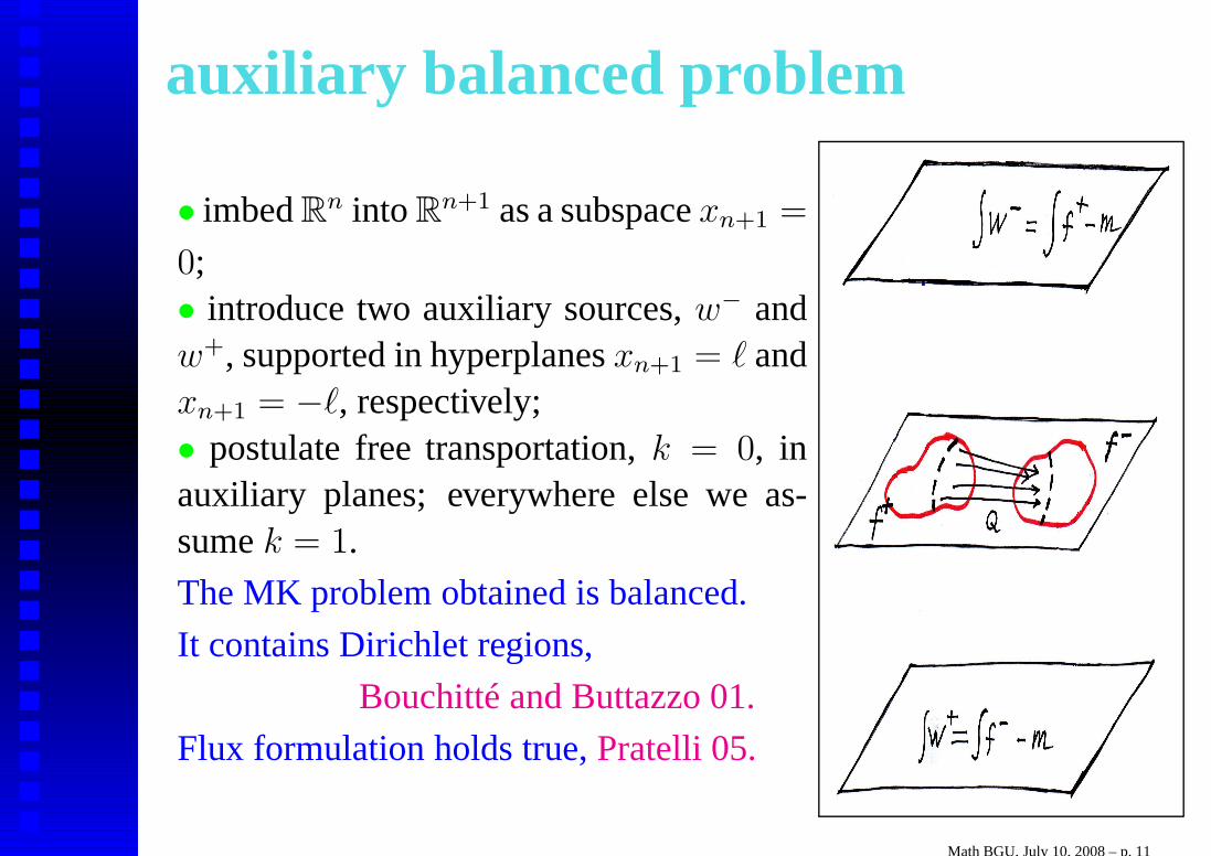
auxiliary balanced problem

• imbedRn into R

n+1 as a subspacexn+1 =

0;• introduce two auxiliary sources,w− andw+, supported in hyperplanesxn+1 = ℓ andxn+1 = −ℓ, respectively;• postulate free transportation,k = 0, inauxiliary planes; everywhere else we as-sumek = 1.

The MK problem obtained is balanced.

It contains Dirichlet regions,

Bouchitté and Buttazzo 01.

Flux formulation holds true,Pratelli 05.

Math BGU, July 10, 2008 – p. 11

auxiliary balanced problem

• Transport in auxiliary planes is free;• If ℓ > ℓ0 = 1

2maxd

Ω(x,y) :

x ∈ spt(f+), y ∈ spt(f−)

transport fromf+ to f− via an

auxiliary plane is not paying;

• The cost of interplane transport is the

same for all reasonable plans.

If q is an optimal flux,Q is a solution to the

partial problem. Flux formulation

min∫∫∫

Ω×[−ℓ,ℓ]k|q| : ∇ · q = f

can be simplified.

Math BGU, July 10, 2008 – p. 12

new variational formulationProblem (PMK):

minKP

∫

Ω

|Q| + ℓ(|q+| + |q−|)

whereKP ⊂ V M0 × [M(Ω)]2 is the set

of triplesQ, q+, q− satisfying three mass

balance conditions (from∇ · q = f ):

∇ · Q + q+ − q− = f+ − f−

∫

Ω

q+ =

∫

Ω

f+ − m,

∫

Ω

q− =

∫

Ω

f− − m

V M0 =

v ∈ [M(Ω)]n : ∃w ∈ M(Ω)

s.t. 〈w,ϕ〉 = −〈v,∇ϕ〉 ∀ϕ ∈ C1(Ω)

.

Math BGU, July 10, 2008 – p. 13

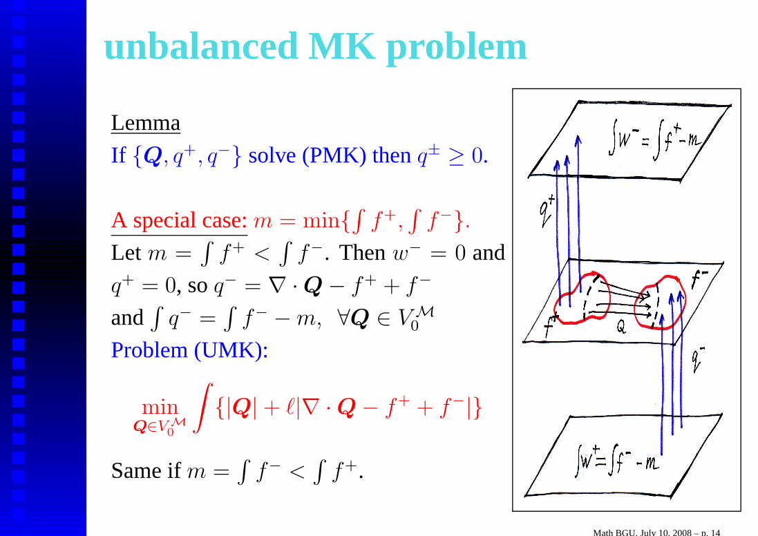
unbalanced MK problem

Lemma

If Q, q+, q− solve (PMK) thenq± ≥ 0.

A special case:m = min∫

f+,∫

f−.

Let m =∫

f+ <∫

f−. Thenw− = 0 and

q+ = 0, soq− = ∇ · Q − f+ + f−

and∫

q− =∫

f− − m, ∀Q ∈ V M0

Problem (UMK):

minQ∈V M

0

∫|Q| + ℓ|∇ · Q − f+ + f−|

Same ifm =∫

f− <∫

f+.

Math BGU, July 10, 2008 – p. 14

back to balanceIn the balanced case,m =

∫f+ =

∫f−, the fluxes

q+, q− are zero. Hence∇ · Q = f+ − f− and wereturn to the known flux formulation,

minQ∈V M

0

∫|Q|

∣∣∣∣ ∇ · Q = f+ − f−

However, for anyℓ > ℓ0 we have also

minQ∈V M

0

∫|Q| + ℓ|∇ · Q − f+ + f−|

as an equivalent flux formulation of L1 MK problem.

Math BGU, July 10, 2008 – p. 15

partial MK problem: existence• Regularization:| · | ≈ 1

r| · |r, where0 < r − 1 ≪ 1;

• For anyr > 1 the Euler-Lagrange equations for regularized

problem have a unique solution:

the fluxesQr ∈ V r0 , q±r ∈ Lr(Ω) and

Lagrange multipliersur ∈ LpI(Ω), λ±

r ∈ R.

Herep = rr−1

, LpI(Ω) = φ ∈ Lp(Ω) :

∫Ω

φ = 0,

V r0 = v ∈ [Lr(Ω)]n : ∇ · v ∈ Lr(Ω), v · ν = 0 on∂Ω.

• As r → 1 the solutions converge (for a subsequence) to a

solution of Euler-Lagrange inequality system associated

with the partialL1 MK problem.

Math BGU, July 10, 2008 – p. 16

numerical solutionApproximation:

• regularization: | · | ≈ 1r| · |r where0 < r − 1 ≪ 1;

• constraint optimization: augmented Lagrangian method;

• discretisation: Raviart-Thomas elements of the least order

and vertex sampling on nonlinear terms forQr, piecewise

constant elements forq±r and the Lagrange multiplierur of

the pointwise constraint;

The convergence is proved.

Implementation:• nonlinearity : iterations, successive over-relaxation;

• singularities: adaptive mesh generation.

Math BGU, July 10, 2008 – p. 17

partial MK: ex. 1

The distributionsf+ andf− are constant in their supports, the left and right ellipses,resp., have

the same total mass, andm = 1

2

∫f+ = 1

2

∫f−. The optimal transport paths are horizontal.

Shown: arrows - calculated flux, ’–’ - computed free boundaries; ’·’ - the position of exact

boundaries. The error of computed optimal transportation cost is less than 0.2% (≈9000 f.e.)

Math BGU, July 10, 2008 – p. 18

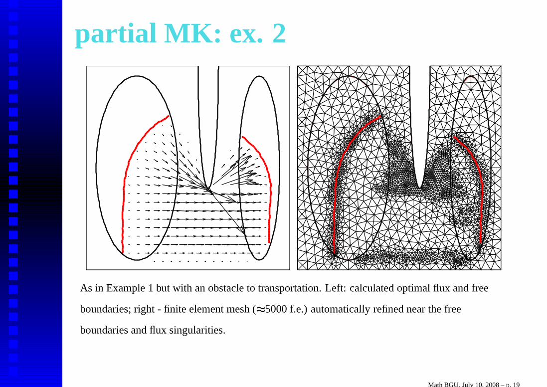
partial MK: ex. 2

As in Example 1 but with an obstacle to transportation. Left:calculated optimal flux and free

boundaries; right - finite element mesh (≈5000 f.e.) automatically refined near the free

boundaries and flux singularities.

Math BGU, July 10, 2008 – p. 19

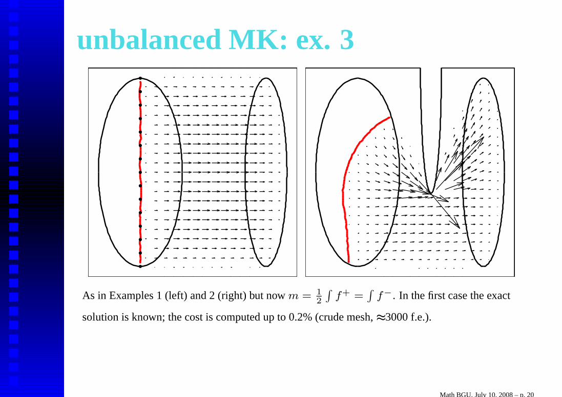
unbalanced MK: ex. 3

As in Examples 1 (left) and 2 (right) but nowm = 1

2

∫f+ =

∫f−. In the first case the exact

solution is known; the cost is computed up to 0.2% (crude mesh, ≈3000 f.e.).

Math BGU, July 10, 2008 – p. 20

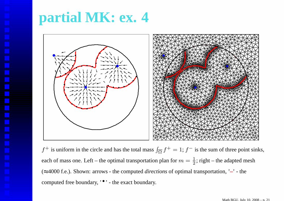
partial MK: ex. 4

f+ is uniform in the circle and has the total mass∫Ω

f+ = 1; f− is the sum of three point sinks,

each of mass one. Left – the optimal transportation plan form = 1

2; right – the adapted mesh

(≈4000 f.e.). Shown: arrows - the computeddirections of optimal transportation, ’–’ - the

computed free boundary, ’·’ - the exact boundary.

Math BGU, July 10, 2008 – p. 21

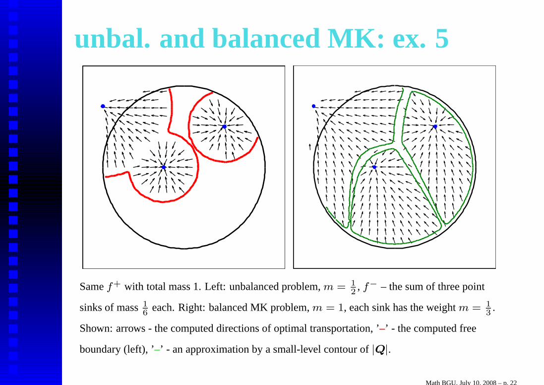
unbal. and balanced MK: ex. 5

Samef+ with total mass 1. Left: unbalanced problem,m = 1

2, f− – the sum of three point

sinks of mass16

each. Right: balanced MK problem,m = 1, each sink has the weightm = 1

3.

Shown: arrows - the computed directions of optimal transportation, ’–’ - the computed free

boundary (left), ’–’ - an approximation by a small-level contour of|Q|.

Math BGU, July 10, 2008 – p. 22

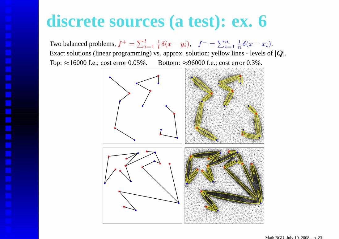
discrete sources (a test): ex. 6Two balanced problems,f+ =

∑li=1

1

lδ(x − yi), f− =

∑ni=1

1

nδ(x − xi).

Exact solutions (linear programming) vs. approx. solution; yellow lines - levels of|Q|.

Top: ≈16000 f.e.; cost error 0.05%. Bottom:≈96000 f.e.; cost error 0.3%.

Math BGU, July 10, 2008 – p. 23

optimal matching problemThe problem studied (for quadratic cost function) inEkeland, 05:

To manufacture a "final product", severalkinds of goods should be brought together;their distributions are measuresf i ∈ M+,i = 1, I with the same totals,

∫f i = m.

What is the matching distributiong ∈ M+,such that

∫g = m and optimal transportation

of all f i ontog is the cheapest?

To solve a partial version of this problem inL1 caseone can use the unbalanced formulation of MKproblem.

Math BGU, July 10, 2008 – p. 24

partial optimal matchingOnly m ≤ min

∫f i units of the final product should

be produced; the distributionsf i may have differenttotal masses.We assume again the transport is insideΩ, sptf i ⊂ Ω,and also that matching is allowed only insideΩ

g⊂ Ω.

The problem (PM):

minI∑

i=1

∫

Ω

|Qi| + ℓ|∇ · Qi − f i + g|

over allQi ∈ V M0 andg ∈ M+(Ω

g),

∫g = m.

Existence: under additional constraintg ≤ G, whereG ≥ m/|Ωg| a given constant.

Math BGU, July 10, 2008 – p. 25

partial matching: ex. 7

f1 andf2 are uniform in the left and right ellipses, resp.,m = 1

2

∫f1 = 1

2

∫f2 = 0.045π;

Ωg is the rectangle in the middle. Left: the constraintg ≤ 1 remains inactive, the optimal

transportation is along the horizontal paths (it is not unique; the choice is made by regularization).

Right: solved forg ≤ m/|Ωg|, so all matching domain must be used to full capacity. Shown:

arrows - the computed optimal flux, ’–’ - the computed free boundary.Math BGU, July 10, 2008 – p. 26

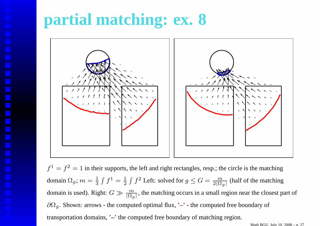
partial matching: ex. 8

f1 = f2 = 1 in their supports, the left and right rectangles, resp.; thecircle is the matching

domainΩg ; m = 1

3

∫f1 = 1

2

∫f2 Left: solved forg ≤ G = m

2|Ωg |(half of the matching

domain is used). Right:G ≫ m|Ωg|

, the matching occurs in a small region near the closest part of

∂Ωg . Shown: arrows - the computed optimal flux, ’–’ - the computed free boundary of

transportation domains, ’–’ the computed free boundary of matching region.Math BGU, July 10, 2008 – p. 27

Reference:J.W. Barrett and L. PrigozhinPartialL1 Monge-Kantorovich problem: Variationalformulation and numerical approximation.Preprint at: www.math.bgu.ac.il/∼leonid

Thank you!

Math BGU, July 10, 2008 – p. 28