particle based modeling of granular-fluid mixtures: … · introduction the model stokes ow fluid...

Introduction The model Stokes ow Fluid Forces Coupling Seabed sediments simulation Conclusions

Particle based modeling of granular-uid mixtures:from porous media to suspensions via solid-uid

transition

Bruno Chareyre (Grenoble INP - 3SR)Emanuele Catalano (Grenoble INP - 3SR)Anh Tuan Tong (Grenoble INP - 3SR)Eric Barthélémy (Grenoble INP - LEGI)

Granulaires Immergés et Suspensions en ECoulement - GISEC33Pessac, Nov. 21th 2011

1/40


Introduction

Discrete elements modeling (DEM) becomes a standard tool forstudying the behavior of (dry) geomaterials at the microscale.

Modern problems involve couplings with intersticial uids, andDEM-based hydromechanical models are being developped actively.

Ecient numerical methods have been proposed to simulate surfacetension eects in two-phase problems (see e.g. Sholtès et al. 2009).

For uid ow however, the proposed methods are eitherover-simplifying or computationaly high-demanding, even for asingle uid.

We propose a new approach, that we apply to one-phaseincompressible Stokes ow as a rst step.

2/40


1 IntroductionFluid - Particles coupling models

2 The modelSpatial partitioning : a key aspect

3 Stokes owAnalytical formulationFlux predictions

4 Fluid ForcesAnalytical Formulation

5 CouplingAlgorithmThe Terzaghi's problem

6 Seabed sediments simulationMotivationSimulated wave action

7 Conclusions

3/40


Layout







7 Conclusions4/40


Fluid - Particles coupling

Continuum Flow Models

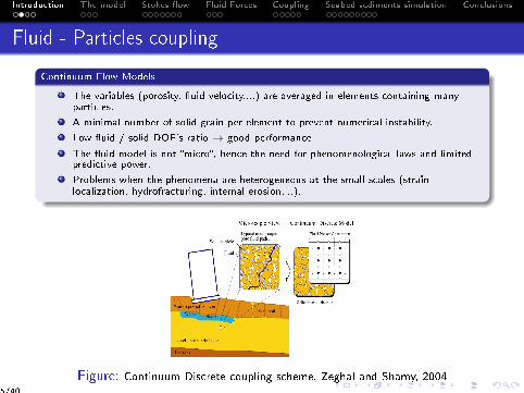
The variables (porosity, uid velocity,...) are averaged in elements containing manyparticles.

A minimal number of solid grain per element to prevent numerical instability.

Low uid / solid DOF's ratio → good performance.

The uid model is not micro, hence the need for phenomenological laws and limitedpredictive power.

Problems when the phenomena are heterogeneous at the small scales (strainlocalization, hydrofracturing, internal erosion,...).

Figure: Continuum-Discrete coupling scheme. Zeghal and Shamy, 20045/40


Fluid - Particles coupling

Microscale uid models (LBM, FEM, FVM,...)

Mesh size particles sizes.

High uid / solid DOF's ratio

Small number of particles

In principle, only classical uid mechanics is introduced (Navier Stokes / Stokes)

Commonly restricted to 2D models, where tricks are needed to let the uid ow (hencekilling the previous advantage...)

Figure: Coupled DEM - LBM method. Han and Feng, 20076/40


Fluid - Solid coupling

Pore scale Finite Volumes Model (PFV)

Fluid / solid DoF's ratio ' 1

Preserves the discrete nature of DEM modelsOnly classical uid mechanics

Hundred thousands of particles in 3D

Figure: Pore scale Finite Volumes model.

7/40


Layout







7 Conclusions8/40


Fluid phase

Regular triangulation

Regular triangulation of particles (onetethraedron = one pore in 3D)

Voronoi tessellation

The dual Voronoi represents a map of thepore space, i.e. path for the uid.

Finite Volumes Formulation

Deforming mesh, following the deformationof the solid phase.One value of pressure per pore (piecewiseconstant eld).

Delaunay Triangulation.

9/40


Fluid phase






Deforming mesh, following the deformationof the solid phase.One value of pressure per pore (piecewiseconstant eld).

Voronoi Tessellation.

9/40


Fluid phase






Deforming mesh, following the deformationof the solid phase.One value of pressure per pore (piecewiseconstant eld). The PFV model.

9/40


Regular vs. Delaunay triangulation

10/40


Layout







7 Conclusions11/40


Analytical Formulation - Flow

Mass conservation

∀cell →∂ρf∂t

+∇ · ρf ~u = 0 (1)

Deformable networkIncompressible uid

⇒∂Vf

∂t+

∫∂Ω

(~uf − ~uΣ) · ~ndS = 0 (2)

In discrete form :

⇒dVf

dt+

∑facets

(~uf ,k ·~n−~uΣ,k ·~n) ·Sk = 0 (3)

Fluid exchanged between pores∑facets

(~uf ,k · ~n − ~uΣ,k · ~n) · Sk =∑

neighbours,i

qi,j (4)

12/40


Pores and Grains

Local geometry

The geometry of the ow path is rather complex anddoes not dene a closed pipe.

Stokes Flow

Stokes equation implies a linear relation between the pressuremicro-gradient and the ux. Then,

qi,j = gijpi − pj

Li,j(5)

where gij is the local conductance dened for the facet ij .

13/40


Pores and grains

Local geometry

The local geometry of the ow path is rather complex and does notdene a closed pipe.

Figure: Bryant et Blunt 1991Thompson 1997

Flow

Which expression in deningconductivity between neighbouringpores ?

14/40


Pores and Grains 2/

Hagen-Poiseuille

We use generalized Hagen-Poiseuille law to dene localconductivities,

⇒ qi,j =AijR

2hyd

2η

∆P

Li,j(6)

where Aij is the area of the uid interface and Rhyd is thehydraulic radius dened for the facet ij .

⇒ Rhyd =Vuid

Ssolid(7)

15/40


Layout







7 Conclusions16/40


Flux predictions

Boundary conditions

Imposed pressure on top and bottomboundariesImpermeable lateral walls

The results gives Qin = Qout

Comparisons

Numerical results from COMSOLsimulationsExperimental measurements on glassbeads for dierent ne/coarse grainsizes ratio (A.T.Tong, PhD inLab3SR)

Pressure elds

17/40


Flux predictions

Boundary conditions



Comparisons


Pressure elds

Solution FEM (a) and PFV (b)

17/40


Flux predictions

Boundary conditions



Comparisons


Pressure elds

Pressure/velocity (top) and pressuregradient (bottom)

17/40


Layout







7 Conclusions18/40


Analytical formulation - Forces

Forces on particles(Chareyre et al., Transport in Porous Media 2011, in press

Force on particle k :

F k =

∫δΓ

k

(p · n + τ · n)ds =

∫δΓ

k

(ρgz + p∗ + τ)nds (8)

Buoyancy force

Fb =

∫δΓ

k

ρgznds (9)

Pressure forces resultant, obtained by consideringpiecewise constant pressure

Fp =

∫δΓ

k

p∗nds = Akij∆pij~nij (10)

Viscous forces resultant, obtained by momentumconservation ⇒ divσ → 0

F v =

∫δΓ

k

τnds = Afij (pj − pi )nij (11)

19/40


Validation of forces denition

Comparison with FEM results

See B. Chareyre et al. Pore-scale Modeling of ViscousFlow and Induced Forces in Dense Sphere Packings,Transport in Porous Media, (in press).

Imposed pressure on top and bottom boundaries.

Impermeable lateral walls.

Forces are extracted and compared for dierentsizes of the small sphere.

20/40


Layout







7 Conclusions21/40


Computation cycle

System to solve

Linearized system to be solved :

[K ]p = ∆V + kimp .pimp (12)

Giving the uid forces :

f w = [G ][K ]−1(∆V + kimp .pimp) (13)

[K ], conductivity matrix (symmetric, sparse, positive dened)

p, pore pressures

∆V , pores' volumetric deformation rate

22/40


Layout







7 Conclusions23/40


Oedometric consolidation

Simulation

5000 particles

σ = 5000Pa

k = 3 · 10−7m/s

Coecient of consolidation :

Cv =kEoed

γ(14)

Consolidation time :

Tv =Cv t

H2(15)

Paraview Visualization Tool

24/40


Oedometric consolidation

Simulation

5000 particles

σ = 5000Pa

k = 3 · 10−7m/s

Analytical solution byTerzaghi (1923)

Evolution of interstitialpressure p(z, t)

25/40


Layout







7 Conclusions26/40


Seabed sediment and waves action

Figure: LEGI instrumented channel.

Context

Role of external ow (waves) on the internal deformation (ex. liquefaction) ?

Complex phenomena involved, mobilizes elasto-plastic behaviour in cyclicloading conditions and liquefaction.

National Project C2D2 Hydrofond on seabed sediments and immersedfoundations.

27/40


Layout







7 Conclusions28/40


Seabed sediment and waves action

An idealized wave action

A sinusoidal-shaped pressure prole is imposed on top boundary

A condition of impermeability is imposed on lateral and bottom boundaries

29/40


Seabed Deformation

Inuence of the initial state

The amplitude of the wave A is increased linearly with time

The behaviour of an initially dense packing (n ' 0.38) vs. a loose packing(n ' 0.42) is observed

Signicant deformations start at A = 1500Pa in the dense packing, A = 300Pain the loose packing.

Figure: Dense packing.

30/40


Seabed Deformation

Inuence of the initial state

The amplitude of the wave A is increased linearly with time

The behaviour of an initially dense packing (n ' 0.38) vs. a loose packing(n ' 0.42) is observed

Signicant deformations start at A = 1500Pa in the dense packing, A = 300Pain the loose packing.

Figure: Loose packing.

31/40


Liquefaction

Figure: Piezometric pressure vs. (x,y) in the dense packing

32/40


Liquefaction

Figure: Piezometric pressure vs. (x,y) in the loose packing

33/40


Seabed Deformation

A more realistic wave action

Seabed loaded by a stationary wave

The scope is to analyze the relation between amplitude and frequency of thewaves, and the evolution of the sediment,...

Figure: Oscillating Waves.

34/40


Conclusions

The model gives correct prediction of permeabilities in spherepackings, refecting the role of porosity and PSD.

The forces induced on individual particles are computed correctly(still limited in terms of size ratio).

The fully coupled scheme is validated in the classical consolidationproblem.

Ecient implementation for large problems, an optimizedtime-integration scheme gave +50% cpu time compared to DEMwithout uid.Up to 500k particles have been simulated in single thread. Thecomputation will be fully parallel in the near future (only partialyparallel a.t.m).

35/40


Computation cycle

System to solve

Linearized system to be solved :

[K ]p = ∆V + kimp .pimp (16)

Giving the uid forces :

f w = [G ][K ]−1(∆V + kimp .pimp) (17)

[K ], conductivity matrix (symmetric, sparse, positive dened)

p, pore pressures

∆V , pores' volumetric deformation rate

36/40


Recent/current researches on the basis of the DEM-PFVcoupling

Extensions and Applications

Interactions between waves and sea-bed sediments (C2D2 ProjectHydrofond supported by MEDDTL, PhD Emanuele Catalano)

Extension to compressible uids for application to high pressureimpacts on concrete structures (PhD thesis Van Tran Tieng,Grenoble)

Extension to dense suspensions and bedload by introducing theeects of shear deformation at the microscale (PhD thesis DoniaMarzougui, Grenoble)

Application to granular lters (transport, plugging), Sari et al., inParticles (2011), Barcelona.

Stability of fractured rock slopes, Donze and Scholtès (2011).

Thermo-chemical eects : methane hydrates dissociation by heatingprocess (Msc thesis Fukuda T., 2010)

37/40


Perspectives and challenges

Particles of complex shapes can be approximated by collections ofspheres (as in fractured rock mass models)

The very active research in the eld of pore-network models maygreatly inspire further extensions to multi-phase ow

The PFV approach in itslef is not restricting the complexity of theow equations : compressibility (already done), inertia, non-linearityat higher Reynolds could be introduced ; at the price of moreassumptions for the pore-upscaling and maybe dierent solvers.

Since the PFV model is assuming dense packings, it should becoupled to a CFD method for boundary value problems includingow outside the porous medium

38/40


Thank you for your attention.

Aknowledgements

Funding : Grenoble INP BQR program, Hydrofond project

supported by MEDDTL in the framework of the C2D2 program.

The PFV coupling is part of the open source project YADE

(http ://yade-dem.org). We thank all contributors to the Yade

project, and users for useful feedback.

39/40


B. Chareyre, A. Cortis, E. Catalano, E. Barthélémy. Pore-scale Modeling of Viscous Flow

and Induced Forces in Dense Sphere Packings. Transport in Porous Media (in press),DOI : 10.1007/s11242-011-9915-6) (2011)

L. Scholtes, B. Chareyre, F. Nicot, F. Darve. Discrete Modelling of Capillary Mechanisms

in Multi-Phase Granular Media. CMES-Computer Modeling in Engineering & Sciences,52(3) :297318, 2009.

H. Sari, B. Chareyre, E. Catalano, P. Philippe, E. Vincens. Investigation of internal

erosion processes using a coupled DEM-Fluid method. Particles 2011 II InternationalConference on Particle-Based Methods, E. Oñate and D.R.J. Owen (Eds), Barcelona(2011)

P.A. Cundall and O.D.L. Strack. A discrete numerical model for granular assemblies.

Geotechnique (1979) 29 :4765.

M Zeghal and U El Shamy. A continuum-discrete hydromechanical analysis of granular

deposit liquefaction Int. J. Numer. Anal. Meth. Geomech. (2004) 14 :(28)13611383.

Bryant S. and Blunt M. Prediction of relative permeability in simple porous media. Phys.

Rev. A (1992) 4 :(46)20042011.

V. Smilauer, E. Catalano, B. Chareyre, S. Dorofeenko, J. Duriez, A. Gladky, J. Kozicki,

C. Modenese, L. Scholtes, L. Sibille, J. Stransky, and K. Thoeni. Yade ReferenceDocumentation. Yade Documentation (V. Smilauer, ed.), The Yade Project, 1st ed.(2010) (http ://yade-dem.org/doc/.)

40/40

particle based modeling of granular-fluid mixtures: … · introduction the model stokes ow fluid...

Documents