particle markov chain monte carlo methods...introduction introduction markov chain monte carlo...
TRANSCRIPT
Particle Markov chain Monte Carlo methods
Meng Li Corey Smith
The Ohio State University
December 7, 2015
Li, Smith PMCMC December 7, 2015 1 / 33

Introduction
Overview
1 Introduction
2 Sequential Monte Carlo
3 Particle Markov Chain Monte Carlo
4 Conclusions
Li, Smith PMCMC December 7, 2015 2 / 33

Introduction
Introduction
Markov chain Monte Carlo (MCMC) methods have become astandard tool for statisticians.
Methods like the Metropolis-Hastings algorithm are commonly usedto sample from high dimensional distributions that may also exhibitcomplex dependency structures.
The efficiency of these algorithms depends on an appropriate choicefor the proposal distribution.
A good proposal distribution should capture important characteristicsof the target distribution, such as its scale and dependence structure.
Li, Smith PMCMC December 7, 2015 3 / 33

Introduction
Introduction
Goal:
Design an efficient proposal distribution.
Problem:
This is a feasible task in small dimensions, but it can be very difficultin high dimensions.
Existing Solutions:
Focus on subcomponents of the target distribution; this can ignoresome of the dependency that exists!
Particle MCMC Solution:
Use sequential Monte Carlo (SMC) and MCMC methods together todesign efficient MCMC algorithms with little user design.
Li, Smith PMCMC December 7, 2015 4 / 33

Sequential Monte Carlo
Overview
1 Introduction
2 Sequential Monte Carlo
3 Particle Markov Chain Monte Carlo
4 Conclusions
Li, Smith PMCMC December 7, 2015 5 / 33
Sequential Monte Carlo
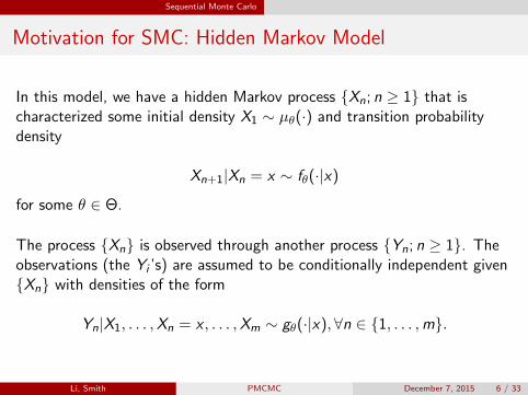
Motivation for SMC: Hidden Markov Model
In this model, we have a hidden Markov process {Xn; n ≥ 1} that ischaracterized some initial density X1 ∼ µθ(·) and transition probabilitydensity
Xn+1|Xn = x ∼ fθ(·|x)
for some θ ∈ Θ.
The process {Xn} is observed through another process {Yn; n ≥ 1}. Theobservations (the Yi ’s) are assumed to be conditionally independent given{Xn} with densities of the form
Yn|X1, . . . ,Xn = x , . . . ,Xm ∼ gθ(·|x),∀n ∈ {1, . . . ,m}.
Li, Smith PMCMC December 7, 2015 6 / 33

Sequential Monte Carlo
Motivation for SMC: Hidden Markov Model
Goal:Perform Bayesian inference conditional on the observationsy1:T = (y1, . . . , yT ) for some T ≥ 1.
This will require the posterior density pθ(x1:T |y1:T ).
If θ ∈ Θ is known, the posterior is proportional to
pθ(x1:T , y1:T ) = µθ(x1)gθ(y1|x1)T∏
n=2
fθ(xn|xn−1)gθ(yn|xn).
If θ ∈ Θ is unknown, the posterior is proportional to
pθ(x1:T , y1:T )p(θ).
Li, Smith PMCMC December 7, 2015 7 / 33
Sequential Monte Carlo
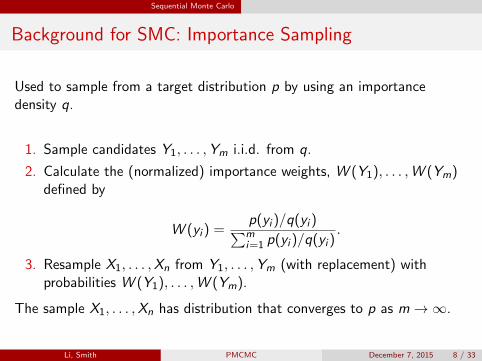
Background for SMC: Importance Sampling
Used to sample from a target distribution p by using an importancedensity q.
1. Sample candidates Y1, . . . ,Ym i.i.d. from q.
2. Calculate the (normalized) importance weights, W (Y1), . . . ,W (Ym)defined by
W (yi ) =p(yi )/q(yi )∑mi=1 p(yi )/q(yi )
.
3. Resample X1, . . . ,Xn from Y1, . . . ,Ym (with replacement) withprobabilities W (Y1), . . . ,W (Ym).
The sample X1, . . . ,Xn has distribution that converges to p as m→∞.
Li, Smith PMCMC December 7, 2015 8 / 33
Sequential Monte Carlo
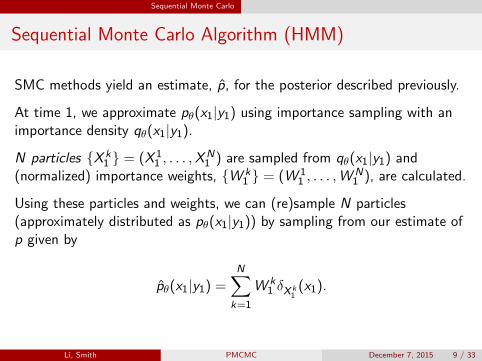
Sequential Monte Carlo Algorithm (HMM)
SMC methods yield an estimate, p̂, for the posterior described previously.
At time 1, we approximate pθ(x1|y1) using importance sampling with animportance density qθ(x1|y1).
N particles {X k1 } = (X 1
1 , . . . ,XN1 ) are sampled from qθ(x1|y1) and
(normalized) importance weights, {W k1 } = (W 1
1 , . . . ,WN1 ), are calculated.
Using these particles and weights, we can (re)sample N particles(approximately distributed as pθ(x1|y1)) by sampling from our estimate ofp given by
p̂θ(x1|y1) =N∑
k=1
W k1 δX k
1(x1).
Li, Smith PMCMC December 7, 2015 9 / 33
Sequential Monte Carlo
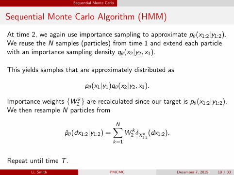
Sequential Monte Carlo Algorithm (HMM)
At time 2, we again use importance sampling to approximate pθ(x1:2|y1:2).We reuse the N samples (particles) from time 1 and extend each particlewith an importance sampling density qθ(x2|y2, x1).
This yields samples that are approximately distributed as
pθ(x1|y1)qθ(x2|y2, x1).
Importance weights {W k2 } are recalculated since our target is pθ(x1:2|y1:2).
We then resample N particles from
p̂θ(dx1:2|y1:2) =N∑
k=1
W k2 δX k
1:2(dx1:2).
Repeat until time T .
Li, Smith PMCMC December 7, 2015 10 / 33
Sequential Monte Carlo
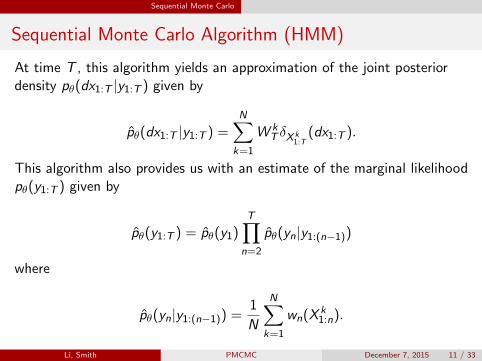
Sequential Monte Carlo Algorithm (HMM)
At time T , this algorithm yields an approximation of the joint posteriordensity pθ(dx1:T |y1:T ) given by
p̂θ(dx1:T |y1:T ) =N∑
k=1
W kT δX k
1:T(dx1:T ).
This algorithm also provides us with an estimate of the marginal likelihoodpθ(y1:T ) given by
p̂θ(y1:T ) = p̂θ(y1)T∏
n=2
p̂θ(yn|y1:(n−1))
where
p̂θ(yn|y1:(n−1)) =1
N
N∑k=1
wn(X k1:n).
Li, Smith PMCMC December 7, 2015 11 / 33
Sequential Monte Carlo
Sequential Monte Carlo: Design and Limitations
This is a powerful algorithm because it requires very little user input,yet still provides useful results.
We need only specify one-dimensional importance densities qθ(x1|y1)and qθ(xn|yn, xn−1) for n ≥ 2.
The authors suggest using qθ(x1|y1) = µθ(x1) andqθ(xn|yn, xn−1) = fθ(xn|xn−1) for n ≥ 2.
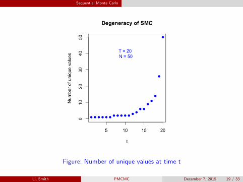
When T is too large, we run into issues of degeneracy.
Successive resampling diminishes the number of distinct values for xn.
Li, Smith PMCMC December 7, 2015 12 / 33

Sequential Monte Carlo
An Illustrative Example: Linear Gaussian SSM
Linear Gaussian State-Space Model
State process {Xt : t ∈ Z}:
Xt = φXt−1 + εt
where εtiid∼ N(0, σ2) and |φ| < 1.
Data process {Yt : t ∈ Z}:
Yt = θXt + rt
where rtiid∼ N(0, γ2).
Parameter vector: θ = (φ, θ, σ2, γ2).
Li, Smith PMCMC December 7, 2015 13 / 33
Sequential Monte Carlo
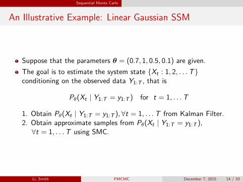
An Illustrative Example: Linear Gaussian SSM
Suppose that the parameters θ = (0.7, 1, 0.5, 0.1) are given.
The goal is to estimate the system state {Xt : 1, 2, . . .T}conditioning on the observed data Y1:T , that is
Pθ(Xt | Y1:T = y1:T ) for t = 1, . . .T
1. Obtain Pθ(Xt | Y1:T = y1:T ), ∀t = 1, . . .T from Kalman Filter.2. Obtain approximate samples from Pθ(Xt | Y1:T = y1:T ),∀t = 1, . . .T using SMC.
Li, Smith PMCMC December 7, 2015 14 / 33
Sequential Monte Carlo
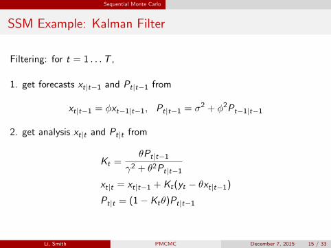
SSM Example: Kalman Filter
Filtering: for t = 1 . . .T ,
1. get forecasts xt|t−1 and Pt|t−1 from
xt|t−1 = φxt−1|t−1, Pt|t−1 = σ2 + φ2Pt−1|t−1
2. get analysis xt|t and Pt|t from
Kt =θPt|t−1
γ2 + θ2Pt|t−1
xt|t = xt|t−1 + Kt(yt − θxt|t−1)
Pt|t = (1− Ktθ)Pt|t−1
Li, Smith PMCMC December 7, 2015 15 / 33
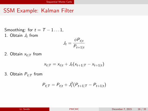
Sequential Monte Carlo
SSM Example: Kalman Filter
Smoothing: for t = T − 1 . . . 1,1. Obtain Jt from
Jt =φPt|t
Pt+1|t
2. Obtain xt|T from
xt|T = xt|t + Jt(xt+1|T − xt+1|t)
3. Obtain Pt|T from
Pt|T = Pt|t + J2t (Pt+1|T − Pt+1|t)
Li, Smith PMCMC December 7, 2015 16 / 33
Sequential Monte Carlo
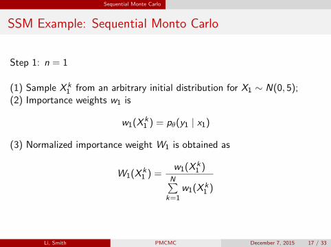
SSM Example: Sequential Monto Carlo
Step 1: n = 1
(1) Sample X k1 from an arbitrary initial distribution for X1 ∼ N(0, 5);
(2) Importance weights w1 is
w1(X k1 ) = pθ(y1 | x1)
(3) Normalized importance weight W1 is obtained as
W1(X k1 ) =
w1(X k1 )
N∑k=1
w1(X k1 )
Li, Smith PMCMC December 7, 2015 17 / 33
Sequential Monte Carlo
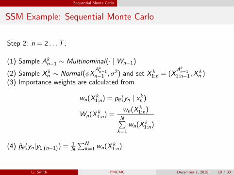
SSM Example: Sequential Monte Carlo
Step 2: n = 2 . . .T ,
(1) Sample Akn−1 ∼ Multinominal(· |Wn−1)
(2) Sample X kn ∼ Normal(φX
Akn−1
n−1 , σ2) and set X k
1:n = (XAkn−1
1:n−1,Xkn )
(3) Importance weights are calculated from
wn(X k1:n) = pθ(yn | xkn )
Wn(X k1:n) =
wn(X k1:n)
N∑k=1
wn(X k1:n)
(4) p̂θ(yn|y1:(n−1)) = 1N
∑Nk=1 wn(X k
1:n)
Li, Smith PMCMC December 7, 2015 18 / 33
Sequential Monte Carlo
Figure: Number of unique values at time t
Li, Smith PMCMC December 7, 2015 19 / 33
Sequential Monte Carlo
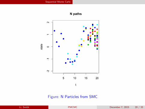
Figure: N Particles from SMC
Li, Smith PMCMC December 7, 2015 20 / 33

Particle Markov Chain Monte Carlo
Overview
1 Introduction
2 Sequential Monte Carlo
3 Particle Markov Chain Monte Carlo
4 Conclusions
Li, Smith PMCMC December 7, 2015 21 / 33
Particle Markov Chain Monte Carlo
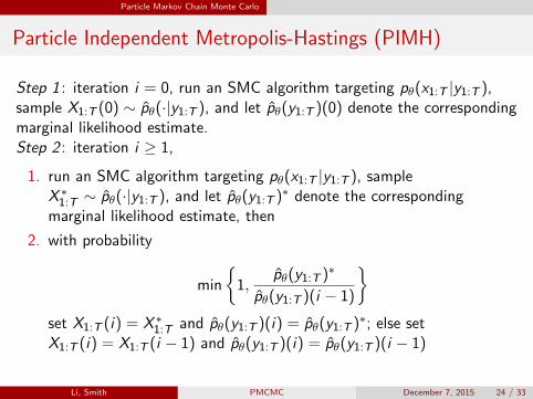
Particle Independent Metropolis-Hastings (PIMH)
PIMH Setup/Notation:
Target Density: pθ(x1:T |y1:T ).
Optimal Proposal Density: qθ(x1:T |y1:T ) = pθ(x1:T |y1:T ).
Realistic Proposal Density: qθ(x1:T |y1:T ) = p̂θ(x1:T |y1:T ).
Implementing p̂θ into the Metropolis-Hastings algorithm yields arelatively simple and familiar method.
Li, Smith PMCMC December 7, 2015 22 / 33
Particle Markov Chain Monte Carlo
Particle MCMC
SMC is an approximate simulation procedure for the target densitypθ(X1:T | Y1:T ).
The output of an SMC algorithm targeting pθ(X1:T | Y1:T ) usingN ≥ 1 particles is used as the proposal distribution for the usualMCMC algorithm.
This cannot be implemented directly, as the evaluation of theacceptance ratio in MCMC requires the marginal density of a particlethat is generated from an SMC algorithm.
Li, Smith PMCMC December 7, 2015 23 / 33
Particle Markov Chain Monte Carlo
Particle Independent Metropolis-Hastings (PIMH)
Step 1 : iteration i = 0, run an SMC algorithm targeting pθ(x1:T |y1:T ),sample X1:T (0) ∼ p̂θ(·|y1:T ), and let p̂θ(y1:T )(0) denote the correspondingmarginal likelihood estimate.Step 2 : iteration i ≥ 1,
1. run an SMC algorithm targeting pθ(x1:T |y1:T ), sampleX ∗1:T ∼ p̂θ(·|y1:T ), and let p̂θ(y1:T )∗ denote the correspondingmarginal likelihood estimate, then
2. with probability
min
{1,
p̂θ(y1:T )∗
p̂θ(y1:T )(i − 1)
}set X1:T (i) = X ∗1:T and p̂θ(y1:T )(i) = p̂θ(y1:T )∗; else setX1:T (i) = X1:T (i − 1) and p̂θ(y1:T )(i) = p̂θ(y1:T )(i − 1)
Li, Smith PMCMC December 7, 2015 24 / 33

Particle Markov Chain Monte Carlo
10 paths from prior state process
t
Prio
r Sta
tes
5 10 15 20-3
-11
23
5 10 15 20
-2-1
01
2
10 paths from posterior process
t
Posterior
Li, Smith PMCMC December 7, 2015 25 / 33
Particle Markov Chain Monte Carlo
0.0 0.5 1.0 1.50.0
0.5
1.0
1.5
t = 1
Density
blue -- Kalman Filter red -- PIMH
-1.0 -0.5 0.0 0.5 1.0
0.0
0.5
1.0
1.5
t = 5
Density
-2.0 -1.5 -1.0 -0.5
0.0
0.4
0.8
1.2
t = 10
Density
-2.0 -1.5 -1.0 -0.5 0.00.0
0.4
0.8
1.2
t = 20
Density
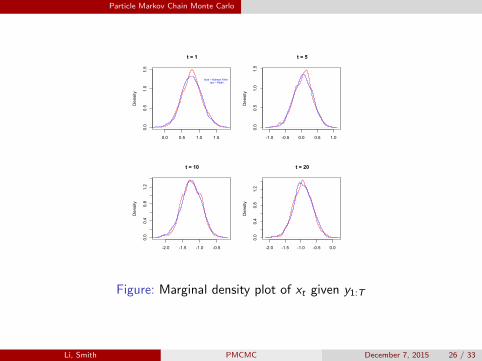
Figure: Marginal density plot of xt given y1:T
Li, Smith PMCMC December 7, 2015 26 / 33
Particle Markov Chain Monte Carlo
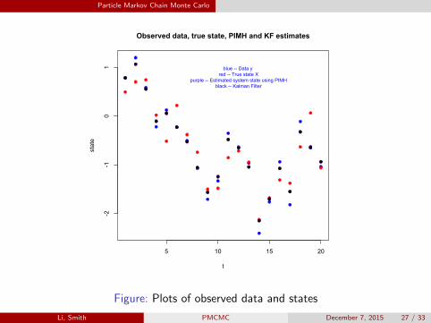
5 10 15 20
-2-1
01
Observed data, true state, PIMH and KF estimates
t
state
blue -- Data y red -- True state X
purple -- Estimated system state using PIMH black -- Kalman Filter
Figure: Plots of observed data and states
Li, Smith PMCMC December 7, 2015 27 / 33
Particle Markov Chain Monte Carlo
Particle MCMC with unknown θ
When the parameter θ is unknown and we are interested in sampling fromp(θ, x1:T |y1:T ),
1. Particle Marginal Metropolis-Hastings Sampling(PMMH)
2. Particle Gibbs Sampling.
Li, Smith PMCMC December 7, 2015 28 / 33
Particle Markov Chain Monte Carlo
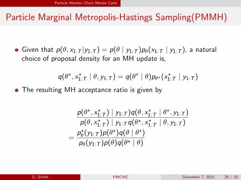
Particle Marginal Metropolis-Hastings Sampling(PMMH)
Given that p(θ, x1:T |y1:T ) = p(θ | y1:T )pθ(x1:T | y1:T ), a naturalchoice of proposal density for an MH update is,
q(θ?, x?1:T | θ, y1:T ) = q(θ? | θ)pθ?(x?1:T | y1:T )
The resulting MH acceptance ratio is given by
p(θ?, x?1:T ) | y1:T )q(θ, x?1:T | θ?, y1:T )
p(θ, x?1:T ) | y1:Tq(θ?, x?1:T | θ, y1:T )
=p?θ(y1:T )p(θ?)q(θ | θ?)
pθ(y1:T )p(θ)q(θ? | θ)
Li, Smith PMCMC December 7, 2015 29 / 33
Particle Markov Chain Monte Carlo
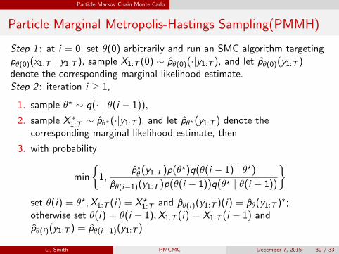
Particle Marginal Metropolis-Hastings Sampling(PMMH)
Step 1 : at i = 0, set θ(0) arbitrarily and run an SMC algorithm targetingpθ(0)(x1:T | y1:T ), sample X1:T (0) ∼ p̂θ(0)(·|y1:T ), and let p̂θ(0)(y1:T )denote the corresponding marginal likelihood estimate.Step 2 : iteration i ≥ 1,
1. sample θ? ∼ q(· | θ(i − 1)),
2. sample X ∗1:T ∼ p̂θ?(·|y1:T ), and let p̂θ?(y1:T ) denote thecorresponding marginal likelihood estimate, then
3. with probability
min
{1,
p̂?θ(y1:T )p(θ?)q(θ(i − 1) | θ?)
p̂θ(i−1)(y1:T )p(θ(i − 1))q(θ? | θ(i − 1))
}set θ(i) = θ?,X1:T (i) = X ?
1:T and p̂θ(i)(y1:T )(i) = p̂θ(y1:T )∗;otherwise set θ(i) = θ(i − 1),X1:T (i) = X1:T (i − 1) andp̂θ(i)(y1:T ) = p̂θ(i−1)(y1:T )
Li, Smith PMCMC December 7, 2015 30 / 33

Conclusions
Overview
1 Introduction
2 Sequential Monte Carlo
3 Particle Markov Chain Monte Carlo
4 Conclusions
Li, Smith PMCMC December 7, 2015 31 / 33
Conclusions
Conclusions
1. In high dimensions, designing an efficient MCMC algorithm (proposal)”by hand” is not possible.
2. Breaking up the problem into many low dimensional problems oftenfails to include some information about the target density.
3. Combining sequential Monte Carlo methods with existing MCMCalgorithms breaks the high dimensional problem in many lowdimensional problems while still accounting for properties of thetarget distribution.
4. Particle MCMC methods provide efficient algorithms with little userdesign needed.
Li, Smith PMCMC December 7, 2015 32 / 33
Conclusions
References
Andrieu and A. Doucet and R. Holenstein (2010), Particle Markovchain Monte Carlo methods, Journal of the Royal Statistical Society,Series B, 72 269-342.
C. K. Wikle and L. M. Berliner (2007), A Bayesian tutorial for dataassimilation, Physica D, 230, 1-16.
Li, Smith PMCMC December 7, 2015 33 / 33