passive and active standoff infrared detection of bio
TRANSCRIPT

PASSIVE AND ACTIVE STANDOFF INFRARED DETECTION OF BIO-AEROSOLS
C.M. Gittins, L.G. Piper, W.T. Rawlins, and W.J. MarinelliPhysical Sciences Inc.
James O. Jensen and Agnes N. AkinyemiUS Army ERDEC
Field Analytical Chemistry and Technology, 3(4-5) (1999).
Copyright © 1999 John Wiley & Sons
Reproduced with permission of John Wiley & Sons, Inc.

PASSIVE AND ACTIVE STANDOFF INFRARED DETECTION OF BIO-AEROSOLS
C.M. Gittins, L.G. Piper, W.T. Rawlins, and W.J. Marinelli*
Physical Sciences Inc.
20 New England Business Center
Andover, MA 01810
James O. Jensen and Agnes N. Akinyemi
US Army ERDEC
ATTN SCBRD RTE / E5554
APG, MD 21010-5423
*Corresponding author.
1
ABSTRACT
Biological compounds are known to have infrared spectra indicative of specific functional
groups. There is a strong interest in the use of passive means to detect airborne biological
particles, such as spores and cells, which may act as biological weapons. At the sizes of interest,
the infrared spectra of bacterial particles results from a combination of geometric (�dparticle > �)
and Mie (�dparticle ~ �) scattering processes while the infrared spectrum of atmospheric particles
falls into the Rayleigh limit (�dparticle << �). In this paper we report on laboratory measurements
of the infrared spectra of aerosolized Bacillus subtilis (BG) spores in air under controlled
measurement conditions. Transmission measurements show an IR spectrum of the spores with
features comparable to the condensed phase spectrum superimposed on a background of Mie
scattering. Preliminary measurements indicate a peak extinction coefficient of approximately
1.6 x 10⁻⁸ cm2 per spore at 9.65 µm. These results are discussed in terms of their implication for
passive and active infrared detection and identification of bio-aerosols.
Keywords: LIDAR, scattering, biological, infrared, passive, extinction

2
1. INTRODUCTION
Vibrational spectroscopy of biological warfare (BW) agents has the potential to probe
spores, vegetative cells, toxins, and rickettsia. In this paper we describe initial efforts to exploit
the potential of vibrational spectroscopy to identify and determine the activity of BW agents.
This approach utilizes extinction and scattering measurements to characterize the vibrational
bands of bacterial particles. It may be possible to compare the vibrational band “fingerprint” of
these materials to spectral libraries to afford rapid detection and identification of BW agents, as
well as determine their activity. Though attempts have been made to interpret the infrared
spectra of bacterial cells in terms of specific physical structures, the spectra exhibit the all the
features of a multi-component mixture comprised of complex molecules.1 Naumann has
conducted an extensive review of the infrared spectroscopy of intact cells.2,3 Of particular
importance is the region from 1500 to 1700 cm-1 containing the so-called “amide I” bands, which
are the strongest features in the spectra and contain information about the structures present in
cell proteins. Spectra of apathogenic Bacillus strains show significant features at 1407 and
1605 cm-1, which can be identified as symmetrical and asymmetrical carboxylate bands, as well
as the strong amide I feature at 1653 cm-1 which can be linked to the presence of poly-D-glutamic
acid in the capsule.
In this paper we discuss the results of preliminary measurements of the extinction
coefficient for aerosolized Bacillus subtilis var. niger (BG) spores in the 2.7 to 12 µm
wavelength region. We then relate those measurements to full IR spectrum measurements of
thin films of BG. These measurements are coupled to calculations of Mie scattering for these
particles in order to assess the role of scattering in the measured total extinction. The results of
3
these measurements and calculations are discussed in terms of their importance to both passive
and active standoff biological agent detection.
2. EXPERIMENTAL MEASUREMENTS
2.1 Experiment Configuration
The measurements were conducted in an improvised aerosol chamber in the laboratories
of Physical Sciences Inc. A schematic diagram of the configuration is shown in Figure 1. The
chamber was a 32 x 32 x 80 in. high fiberglass and metal enclosure modified for optical access
across its 32 in. depth. The BG spores were suspended in an aqueous solution and sprayed into
the chamber utilizing an ultrasonic atomizer configured to deliver droplets with a mean diameter
of 20 µm. The solution was metered to the atomizer using a peristaltic pump at a rate of
10 ml/min. A heated supply of ~ 50(C air was delivered to the chamber to break up the flow
from the atomizer, prevent recondensation of water, as well as provide the heat of vaporization
for the injected liquid. The flow rate was set to provide air in the chamber at approximately 50%
relative humidity under ambient laboratory temperature conditions. The chamber pressure was
held at ambient atmospheric through the use of a vent hose connecting the chamber to a fume
hood. The chamber volume divided by the gas flow rate gives a characteristic residence time for
gas in the chamber of approximately 3 min. A recirculating blower system was also available to
provide a well mixed air flow in the chamber. However, we decided that the dilution flow
provided ample mixing in the chamber and this blower was not used in most measurements
because of concerns about sticking of particles in the blower system. Each change of chamber

4
operating conditions was allowed to equilibrate for 15 min (5 residence times) prior to
conducting any optical measurements.
Optical transmission measurements were conducted in the chamber using a MIDAC FTIR
spectrometer at a resolution of 16 cm-1. The chamber afforded a single pass path length of 75 cm.
Two inch windows on either end of the chamber were formed from 3M heat shrinkable
polyethylene window insulation material. In situations where there is no pressure differential
between the chamber and the ambient atmosphere this insulation was found to make a good
window due to its low refractive index and lack absorption bands in the thermal infrared region
(8 to 12 µm). Significant absorptions in the 3.3 and 6.5 µm regions make it unsuitable for some
other investigations.
2.2 Sample Preparation And Concentration Determination
The BG spore samples were prepared from an existing stock simulant solution at U.S.
Army ERDEC. Washed and unwashed samples were used in the reported measurements to
assure the spectra observed were characteristic of the spores rather than residual growth medium
or other contaminant. The spectra measured in this effort showed no difference between the
washed and unwashed samples. The data reported in these measurements utilized an unwashed
sample with a spore concentration of 8.8 x 10⁹ ml-1 as determined by flow cytometry. In this
paper we report extinction measurements on a per spore basis in order to avoid confusion about
the extent of agglomeration in the aerosolization. In determining the spore concentration we
assume steady state conditions. The spore aerosol concentration is simply given by dividing the
spore injection rate (spores per minute) by the dilution air flow rate (cm3 per minute). The spore
injection rate is the product of the spore solution concentration (8.8 x 10⁹ spores/ml) and the

5
liquid injection rate (10 ml/min) or 8.8 x 10¹⁰ spores/min. The gas flow rate was 1855 liters/min
leading to a steady state spore concentration of 4.7 x 10⁴ spores cm-3. Given a 75 cm optical
path, the total column density for the measurements was approximately 3.6 x 10⁶ spores cm-2.
We note that the calculation of the steady state spore column density assumes no losses due to
heterogeneous removal on the walls of the chamber. As such, the cross sections reported here are
lower limits on the actual value.
2.3 Experimental Results
Spore aerosol measurements are conducted by bringing the chamber to steady state using
pure water injection. Under these conditions a series of background spectra of the chamber are
recorded for reference to the spectra recorded under spore injection. Following acquisition of the
background the spore solution is injected into the chamber at the same flow rate as the pure water
and the chamber allowed to equilibrate. Spectra of the aerosolized spores are then recorded and
the chamber injection system returned to pure water. A series of post acquisition background
spectra are recorded to account for baseline drift over the ~ 3/4 hour required for an acquisition
sequence. Figure 2 shows a sequence of spectra recorded during the equilibration of the chamber
following spore injection. The data clearly shows a broad feature growing in with a maximum at
approximately 9.65 µm (1065 cm-1) as well as additional features in the 3.1 µm (~3200 cm-1) and
6.2 µm (~1620 cm-1) regions. Under most conditions these features returned to baseline upon re-
injection of the pure water solution. However, in some experiments spectral features were
observed to persist following the changeover to pure water, probably indicating that window
contamination had occurred. These data were not used in our analysis.
6
Good spore aerosol spectra could be reliably obtained throughout the IR region, except
for the window absorption bands. The transmission measurements were used to determine the
extinction coefficient. The spectra were converted to absorbance units (base e) using Beer’s law.
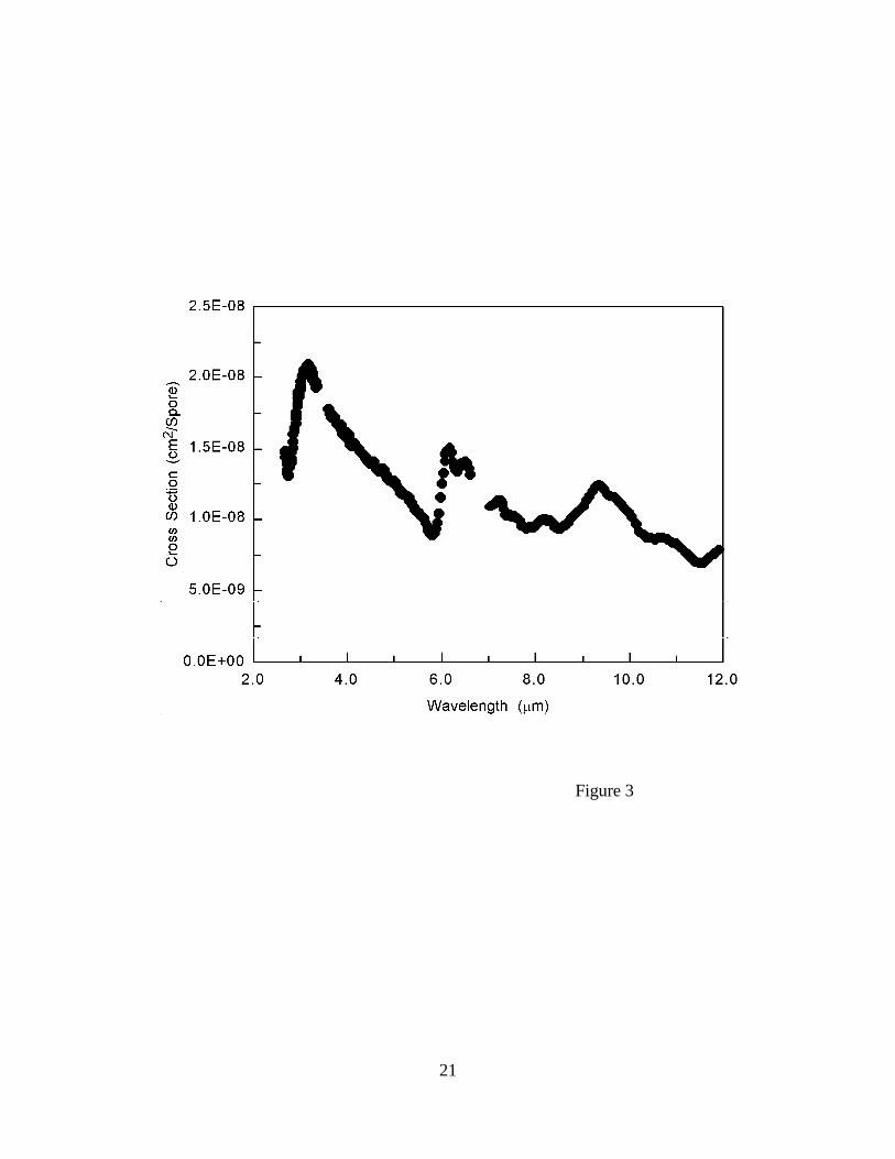
The absorbance data was converted to extinction cross sections using the column density
assumed from the steady state analysis presented above. The results of this analysis are shown in
Figure 3 for the region from 2.7 to 12 µm. The thin film transmission measurement is shown in
Figure 4 as converted to absorbance units (base e). These measurements extend from 2 to
approximately 14 µm. The spectral features are quite similar to the Bacillus subtilis spectra
reported by Naumann2.
3. DATA INTERPRETATION
3.1 Interpretation of Thin Film Spectra
The similarity between the thin film spectrum and the aerosol spectrum gives us some
leeway in trying to relate the two pieces of data. The features in both spectra at 3.1 µm are
clearly identified as the “amide A” bands.2 The methyl stretching mode band in the aerosol
spectrum is obscured by a window absorption band. Similarly, the “amide I” and “amide II”
bands in the 5.5 to 8 µm region are also evident in both spectra, although partially obscured by
another window absorption in the aerosol measurement. The feature at 9.65 µm can be attributed
to bands associated with either a phosphodiester or polysaccharide.
To understand the utility of these features for standoff detection of bio-aerosols we also
calculated the atmospheric transmission spectrum for a 10 km path at sea level and calculated the
product of the two spectra to establish the spectral regions of utility for remote sensing applica-
7
ûN 2atm1spore! KûT � NESR (1)
tions. It is clear from the scaled data and the atmospheric transmission spectrum that the infrared
regions from 8 to 13 µm and from 3.0 to 4.0 µm are key to standoff detection of the BG spore
aerosols. Unfortunately, the region from 5.5 to 8.0 µm, which contains significant differentiating
features in the spectrum, is obscured by atmospheric water absorptions. In the remainder of this
paper we consider three standoff detection approaches: passive detection in the 8 to 12 µm band,
active detection in the 9 to 11 µm region using CO2 laser DIAL or DISC approaches, and
differential scattering in the 1.5 and 3.5 µm region using the signal and idler from an OPO-based
LIDAR system.
3.2 Passive Standoff Detection Approaches
The ability of a sensor to detect any biological or chemical cloud depends on the apparent
radiance contrast due to the presence of the cloud compared to the noise-equivalent spectral
radiance (NESR) of the sensor employed. In simple form, the relationship between the radiance
contrast produced by the cloud and the sensor NESR is given by the expression:
where ûN is the radiance differential due to the presence of the cloud, 2atm is the atmospheric
transmission between the cloud and the sensor (~65%), 1spore is the absorption cross section on a
per spore basis (1.6 x 10⁻⁹ cm2 spore-1), ! is the spore column density, K is the derivative of the
radiance with respect to temperature (~ 1.5 x 10⁻⁵ W cm-2 sr-1 µm-1 K-1 ) at the sensor wavelength
(9.65 µm), and ûT is the apparent temperature difference between the cloud and the background.
In these calculations we assume a low-sky ûT of 21K. Typical sensor NESR values range from
10-6 to 10-7 W cm-2 sr-1 µm-1. The differential radiance as a function of spore concentration is

8
shown in Figure 5 for a path length of 100 m through the cloud. The calculations show that the
differential radiance does not exceed the sensor NESR until a spore concentration of ~4 per cm3
is reached. Since the spores agglomerate to contain 2 to 10 spores per particle, the sensor NESR
is reached at a particle density of 0.4 to 2 per cm3. However, a significant fraction of the total
cloud extinction is due to broad band scattering. Passive detection methods require that the
sensor be able to sample the unperturbed background radiance from the scene at nearby
wavelengths in order to assess the influence of the biological agent cloud on the transport of
radiation from the scene to the sensor. This underlying broad band scattering component does
not allow the sensor to sample the background radiance free of the influence of the agent cloud.
Hence, as a practical matter the net observable radiance is probably limited to the structured
absorption component of the total extinction cross section. This broadband component has the
effect of reducing the contrast of the cloud in the scene by approximately a factor of two.
It is generally acknowledged that relevant bio-particle densities are in the range from 0.1
to 10 particles per cm3. Hence, based on this preliminary assessment, passive sensing of a bio-
aerosol cloud would appear to be at the limit of current passive detection capabilities Our
calculations suggest field experiments should be conducted to assess the potential of these
devices to detect bio-aerosols.
3.3 LWIR Disc/Dial Lidar
Differential LIDAR approaches generally require 10 to 20 percent absorbances to have
reasonable sensitivity levels.4,5 The transmission spectrum of the cloud from Figure 5 shows a
10% absorbance is not achieved in the 9.65 µm band until the number density exceeds approxi-
9
mately 1000 spores per cm3. Hence, the DIAL approach in the long wavelength infrared (LWIR)
is no more attractive than the passive sensor for most significant applications in bio-detection.
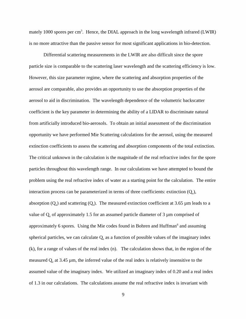
Differential scattering measurements in the LWIR are also difficult since the spore
particle size is comparable to the scattering laser wavelength and the scattering efficiency is low.
However, this size parameter regime, where the scattering and absorption properties of the
aerosol are comparable, also provides an opportunity to use the absorption properties of the
aerosol to aid in discrimination. The wavelength dependence of the volumetric backscatter
coefficient is the key parameter in determining the ability of a LIDAR to discriminate natural
from artificially introduced bio-aerosols. To obtain an initial assessment of the discrimination
opportunity we have performed Mie Scattering calculations for the aerosol, using the measured
extinction coefficients to assess the scattering and absorption components of the total extinction.
The critical unknown in the calculation is the magnitude of the real refractive index for the spore
particles throughout this wavelength range. In our calculations we have attempted to bound the
problem using the real refractive index of water as a starting point for the calculation. The entire
interaction process can be parameterized in terms of three coefficients: extinction (Qe),
absorption (Qa) and scattering (Qs). The measured extinction coefficient at 3.65 µm leads to a
value of Qe of approximately 1.5 for an assumed particle diameter of 3 µm comprised of
approximately 6 spores. Using the Mie codes found in Bohren and Huffman6 and assuming
spherical particles, we can calculate Qe as a function of possible values of the imaginary index
(k), for a range of values of the real index (n). The calculation shows that, in the region of the
measured Qe at 3.45 µm, the inferred value of the real index is relatively insensitive to the
assumed value of the imaginary index. We utilized an imaginary index of 0.20 and a real index
of 1.3 in our calculations. The calculations assume the real refractive index is invariant with

10
n(r) Mn
i1
Ni
ln(10) r 1i 2�x exp
(log r log ri)2
2 12i
(2)
wavelength and the imaginary index is determined from the measured value of Qe at each
wavelength considered.. Using this parameterization we can calculate the differential scattering
cross section using the Mie codes. Although we have no extinction data at 1.55 µm, we expect
the bio-aerosol absorption to be weak since this wavelength region is characterized by overtone
and combination bands. Thus, we have assumed k�0 at this wavelength.
A multi-mode log-normal distribution was used to parameterize both the biological and
atmospheric aerosol distributions. The form of the distribution is given by:
where n is the number of modes, Ni is the fraction of the total distribution in each mode, ri is the
mode radius, and 1i is the mode width. The angular scattering efficiencies were calculated for
the biological and an atmospheric aerosol distributions defined in Table 1. The atmospheric
aerosol distribution was the rural atmospheric aerosol model used in MODTRAN7 which
comprises a small radius water soluble fraction and a larger radius dust-like fraction. The
biological aerosol distribution assumed a 1.5 µm mean radius, based on generally held opinions
on the extent of agglomeration during spore distribution. The mode width was set to assure a
negligible fraction of the distribution occurred at a size below the reported minimum width of a
single spore (0.25 µm). Table 2 shows the values of the real and imaginary indices used in the
scattering calculations for each wavelength.
Figure 6 shows the differential scattering cross sections (cm2 sr-1) calculated for the log-
normal bio-aerosol distribution defined in Table 1 at wavelengths of 1.55, 3.45, and 9.65 µm. A
similar calculation was performed for the rural atmospheric aerosol model used in MODTRAN7
to validate the scattering code. The bio-aerosol calculations correctly predict that the total

11
scattering cross section, as determined by integrating over all scattering angles, scales inversely
with the scattering wavelength. However, the calculations show that virtually all of the enhanced
scattering occurs in the forward direction (0 deg) while, in the backscattering direction important
for LIDAR applications, there are only small differences in the cross section compared to the
forward scattering.
The differential backscattering cross sections can be converted to volumetric
backscattering coefficients (km-1 sr-1) by assuming a particle number density and 1 km path
length. The volumetric backscatter coefficients obtained from this calculation can be compared
with values for the natural atmosphere for the same wavelengths.7 Our code calculations were in
good agreement with these values. The absolute and relative values of the coefficients have
significance for LIDAR detection and discrimination capability. The comparison of the
calculations (as a function of particle density) and natural atmospheric data are shown in
Figure 7. The calculations seem to indicate a trend: the particle number density at which the
volumetric backscatter coefficient for the bio-aerosol equals the natural background is inversely
proportional to wavelength. However, the absolute value of the coefficients decrease with
increasing wavelength. Thus, the ability to detect any aerosol signal improves at shorter
wavelengths. However, the ability to detect a bio-aerosol against the natural background should
improve at longer wavelengths.
Additional insight is obtained by comparing the ratio of volumetric backscatter
coefficients as a function of wavelengths for the two different aerosols. This information is
shown, normalized to the values at 1.55 µm, in Table 3. The initial conclusion from reviewing
these ratios is that the OPO signal/idler ratio appears to provide little discrimination capability in
LIDAR applications. Though there are significant differences in the total extinction cross

12
sections for the two wavelengths, these differences appear to manifest all in the forward
scattering direction. However, the comparison also shows that some discrimination capability
may be provided by comparing returns from a dual OPO/CO2 LIDAR system, i.e., 1.55 versus
9.65 µm. This apparent discrimination capability may arise from two factors: 1) the sampling of
a bio- aerosol distribution with a mean diameter of 3 µm compared to an atmospheric aerosol
with a size distriubution centered around 0.1 µm, and 2) the enhancement of scattering in the
region near the 9.6 µm absorption band in the bio-aerosol. Larger mean bio-aerosol radii would
tend to enhance these size differences. However, we note that the inferred value of the real index
measured at 9.65 µm (k = 0.39) is approximately 75% larger than the measurements of Querry
reported by Flanigan.8 The sensitivity of the scattering ratios to the measured value of the
extinction coefficient at 9.65 µm suggests that confirmatory backscattering measurements are
warranted.
4. CONCLUSIONS
The preliminary results reported in this paper are rendered significantly uncertain by a
lack of understanding of the particle size distribution produced in the ultrasonic generator used to
create the aerosol. Beyond the questions of aerosol generation, there remains a significant
uncertainty in the actual particle/spore number density. The possibility of significant surface
losses in the aerosol chamber makes the resulting extinction cross sections lower limits, at best.
In future measurements we hope to include light scattering measurements which will provide a
measure of actual particle size and density for extinction and laser backscattering measurements.
The existing data indicates that passive measurements of biological agent cloud may be
quite difficult if the extinction cross sections determined in these measurements remain valid.

13
However, we again caution that these data represent lower limits to the actual extinction cross
sections. The scattering calculations suggest that the signal/idler ratio in an OPO-based system
may not provide the ability to discriminate natural atmospheric from bio-aerosols. However, the
ratio of scattered intensities at 1.55 and 9.65 µm may provide that capability, albeit at difficult
signal levels in the 9.65 µm band.
5. REFERENCES
1. D. Naumann, D. Helm, and H. Labischinski, “Microbiological Characterizations by FT-
IR Spectroscopy,” Nature 351, 81-82, (1991).
2. D. Naumann, C.P. Schultz, D. Helm, “What Can Infrared Spectroscopy Tell Us About the
Structure and Composition of Intact Bacterial Cells,” in Infrared Spectrscopy of
Biomolecules, ed. by H.H. Mantsc and D. Chapman, Wiley-Liss, New York, 1996.
3. D. Naumann, D. Helm, H. Labischinski, and P. Giesbrecht, “The Characterization of
Microorganisms by Fourier-Transform Infrared Spectroscopy (FT-IR)” in Modern
Techniques for Rapid Microbiological Analysis, ed. by W.H. Nelson, VCH, New York,
(1991), pp. 43-96.
4. F.M. D’Amico, “Quantitative Vapor Detection with a Multiwavelength CO2 LIDAR,”
Proc. of the 1996 Meeting of the IRIS Specialty Group on Active Systems, 13-16 May
1996, pp. 345-364.
5. D. Dean, J. Blackburn, M. Fox, C. Hamilton, S. Alejandro, M. Stephen, S. Ghoshroy,
Y. Weang, H. Stowe, M. Fava, J, DiMercurio, J. Dowling, M. Kelley, D. Senft, K. Agar,
and M. Shilko, “Design of an Airworthy, Long-Standoff Range Differential Absorption

14
LIDAR Device,” Proc. of the 1996 Meeting of the IRIS Specialty Group on Active
Systems, 13-16 May 1996, pp. 365-384.
6. C. Bohren and D.R. Huffman, Absorption and Scattering of Light by Small Particles,
John Wiley and Sons, New York, 1983.
7. A.S. Jursa, editor, Handbook of Geophysics and the Space Environment, National
Technical Information Service No. ADA 167000, (1985). pp. 18-10 to 18-15.
8. D.F. Flanigan, Hazardous Cloud Imaging: An In-Depth Study, U.S. Army CRDEC
Technical Report ERDEC-TR-416, July 1997.

15
Figure Captions
Figure 1. Schematic diagram of aerosol chamber and optical measurement system used for
BG spore extinction measurements.
Figure 2. Time sequence of transmission spectra recorded during injection of BG spore sample
into the aerosol chamber. The variable feature at 2350 cm-1 is due to atmospheric CO2
absorption and is indicative of some baseline shift.
Figure 3. Extinction cross sections for aerosolized BG spores measured in this effort. Gaps in the
spectrum indicate the location of window material absorption bands.
Figure 4. Absorption spectrum of a thin film of BG spores.
Figure 5. Differential radiance and optical transmission as a function of spore density in a 100 m
cloud. Nominal NESR of typical passive sensor included for reference.
Figure 6. Calculated differential cross section as a function of scattering angle for wavelengths of
1.55, 3.45, and 9.65 µm.
Figure 7. Bio-aerosol and natural aerosol volumetric backscatter coefficients for the three
wavelengths considered in this study. The bio-aerosol values are shown as a function of
the cloud particle density for a 1 km path.
16
Tables
Table 1. Parameters Used in Defining Aerosol Distributions Used in the Scattering Calculations
Aerosol ModelSize Fraction
(Ni) Mode Radius (µm) (ri)Mode Width (µm)
(1i)
Rural
Water-soluble 0.999875 0.03 0.35
Dust-like 0.000125 0.50 0.4
Biological 1.000000 1.50 0.15
17
Table 2. Real (n) and Imaginary (k) Refractive Indices Used in the Scattering Calculations
Wavelength (µm)
1.55 3.45 9.65
Distribution n k n k n k
Rural Aerosol
Water-soluble 1.50 2.0 x 10⁻² 1.45 6.0 x 10⁻³ 2.60 0.4
Dust-like 1.37 9.0 x 10⁻³ 1.26 1.0 x 10⁻² 1.70 0.15
Bio-aerosol 1.30 0.0 1.30 0.2 1.30 0.39

18
Table 3. Comparison of Relative Backscattering Coefficients and Size Parameters as a Function of Wavelength for the Two Aerosol Distributions
Wavelength (µm)
Bio-aerosol Atmospheric Aerosol
Cross SectionRatio
SizeParameter
(2�r/�)Cross Section
Ratio
SizeParameter
(2�r/�)
1.55 1.00 3.87 1.00 0.13
3.45 0.27 1.74 0.42 0.06
9.65 1.05 0.63 0.19 0.02

19
Figure 1
20
Figure 2
21
Figure 3

22
Figure 4

23
Figure 5

24
Figure 6

25
Figure 7

26

27