path planning and control of an autonomous quadrotor
TRANSCRIPT
Graduate Theses, Dissertations, and Problem Reports
2015
Path Planning and Control of an Autonomous Quadrotor Testbed Path Planning and Control of an Autonomous Quadrotor Testbed
in a Cluttered Environment in a Cluttered Environment
Trevor W. Caplinger
Follow this and additional works at: https://researchrepository.wvu.edu/etd
Recommended Citation Recommended Citation Caplinger, Trevor W., "Path Planning and Control of an Autonomous Quadrotor Testbed in a Cluttered Environment" (2015). Graduate Theses, Dissertations, and Problem Reports. 5313. https://researchrepository.wvu.edu/etd/5313
This Thesis is protected by copyright and/or related rights. It has been brought to you by the The Research Repository @ WVU with permission from the rights-holder(s). You are free to use this Thesis in any way that is permitted by the copyright and related rights legislation that applies to your use. For other uses you must obtain permission from the rights-holder(s) directly, unless additional rights are indicated by a Creative Commons license in the record and/ or on the work itself. This Thesis has been accepted for inclusion in WVU Graduate Theses, Dissertations, and Problem Reports collection by an authorized administrator of The Research Repository @ WVU. For more information, please contact [email protected].
Path Planning and Control of an Autonomous Quadrotor
Testbed in a Cluttered Environment
Trevor W. Caplinger
Thesis submitted to the Benjamin M. Statler College of Engineering and Mineral Resources
at West Virginia University
in partial fulfillment of the requirements for the degree of
Master of Science in
Mechanical Engineering
Committee Members
Yu Gu, Ph.D., Chair
Jason Gross, Ph.D.
John Christian, Ph.D.
Powsiri Klinkhachorn, Ph.D.
Department of Mechanical and Aerospace Engineering
Morgantown, West Virginia
2015
Keywords: Quadrotor, Quadcopter, Path Planning, D*, PRM, Control
Copyright 2015 Trevor Caplinger
Abstract
Path Planning and Control of an Autonomous Quadrotor Testbed in a
Cluttered Environment
Trevor W. Caplinger
A classical problem for robotic navigation is how to efficiently navigate from one point to another and what to do if obstacles are encountered along the way. Many map based path planning algorithms attempt to solve this problem, all with varying levels of optimality and complexity. This work shows a review of selected algorithms, and two of these are selected for simulation and testing using a quadrotor unmanned aerial vehicle (UAV) in a dynamic indoor environment which requires replanning capabilities. The Dynamic A* algorithm, or simply D*, and the Probabilistic Roadmap method (PRM) are used in a scenario designed to test their respective functionality and usefulness with the goal of determining the better algorithm for flight testing given a partially known or changing environment.
The development of the quadrotor platform hardware is discussed as well as the associated software and capabilities. Both algorithms are redesigned to fit this specific application and display their respective planned and replanned paths in an intuitive and comparable manner. Simulation is performed and an obstacle is added to the map during the quadrotor motion, requiring a replanned path. Results are compared for both computed path length and computational intensity. Flight testing is performed in an indoor environment, and during the flight an obstacle is inserted into the flight path, requiring detection and replanning. Results are compared for computed path length and intuitively analyzed to compare optimality and complexity.
iii
Acknowledgements
I would like to thank the following people for their outstanding contributions to my
research. I truly could not have done this without you.
Dr. Yu Gu, thank you for believing in me and inviting me to work on your team. Working
with you has been an honor and a learning experience every step of the way. Your guidance
over the last two years has made me a smarter, harder worker. I have learned much from your
quiet openness and intelligence.
Dr. Jason Gross, Dr. John Christian, and Dr. Powsiri Klinkhachorn, thank you for
mentoring and guiding me in my pursuit of knowledge. You have all impacted my life and made
me want to learn more. Thank you all for being on my defense committee.
A big thank you to everyone associated with the Interactive Robotics Laboratory team:
Tanmay Mandal, Kyle Lassak, Yaohui Ding, Jared Strader, Alex Hypes, Caleb Rice, Trenton
Larrabee, Scott Harper, Alex Gray, Srikanth Gururajan. You all helped selflessly and
encouraged generously. Thank you for your friendship and support.
I also want to thank John Hailer for graciously helping when I was in need. Thank you for
the number of hours you selflessly spent to aid me.
Thank you Mom and Dad for always loving me, praying for me and encouraging me in
my education from the time I was born. I hope I honor you for putting me on the path to where I
am now.
Most importantly, to my loving wife Mikaela, thank you for allowing me to pursue this
dream, for being my biggest supporter through it all, and even helping me when I needed extra
hands. You inspire me to succeed, and I hope that I will always return the support and love you
have shown me.
This research was supported in part by NASA Independent Validation & Verification
Facility and NASA WV Space Grant Consortium.
iv
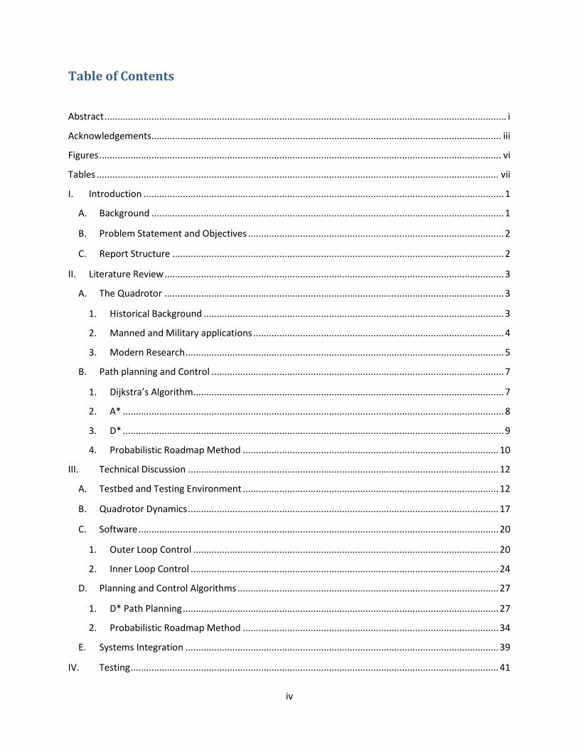
Table of Contents
Abstract .......................................................................................................................................................... i
Acknowledgements ...................................................................................................................................... iii
Figures .......................................................................................................................................................... vi
Tables .......................................................................................................................................................... vii
I. Introduction .......................................................................................................................................... 1
A. Background ....................................................................................................................................... 1
B. Problem Statement and Objectives .................................................................................................. 2
C. Report Structure ............................................................................................................................... 2
II. Literature Review .................................................................................................................................. 3
A. The Quadrotor .................................................................................................................................. 3
1. Historical Background ................................................................................................................... 3
2. Manned and Military applications ................................................................................................ 4
3. Modern Research .......................................................................................................................... 5
B. Path planning and Control ................................................................................................................ 7
1. Dijkstra’s Algorithm ....................................................................................................................... 7
2. A* .................................................................................................................................................. 8
3. D* .................................................................................................................................................. 9
4. Probabilistic Roadmap Method .................................................................................................. 10
III. Technical Discussion ....................................................................................................................... 12
A. Testbed and Testing Environment .................................................................................................. 12
B. Quadrotor Dynamics ....................................................................................................................... 17
C. Software .......................................................................................................................................... 20
1. Outer Loop Control ..................................................................................................................... 20
2. Inner Loop Control ...................................................................................................................... 24
D. Planning and Control Algorithms .................................................................................................... 27
1. D* Path Planning ......................................................................................................................... 27
2. Probabilistic Roadmap Method .................................................................................................. 34
E. Systems Integration ........................................................................................................................ 39
IV. Testing ............................................................................................................................................. 41
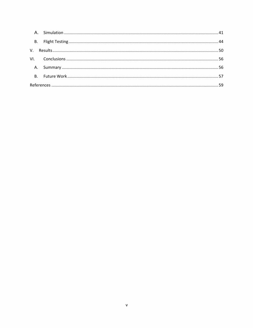
v
A. Simulation ....................................................................................................................................... 41
B. Flight Testing ................................................................................................................................... 44
V. Results ................................................................................................................................................. 50
VI. Conclusions ..................................................................................................................................... 56
A. Summary ......................................................................................................................................... 56
B. Future Work .................................................................................................................................... 57
References .................................................................................................................................................. 59
vi
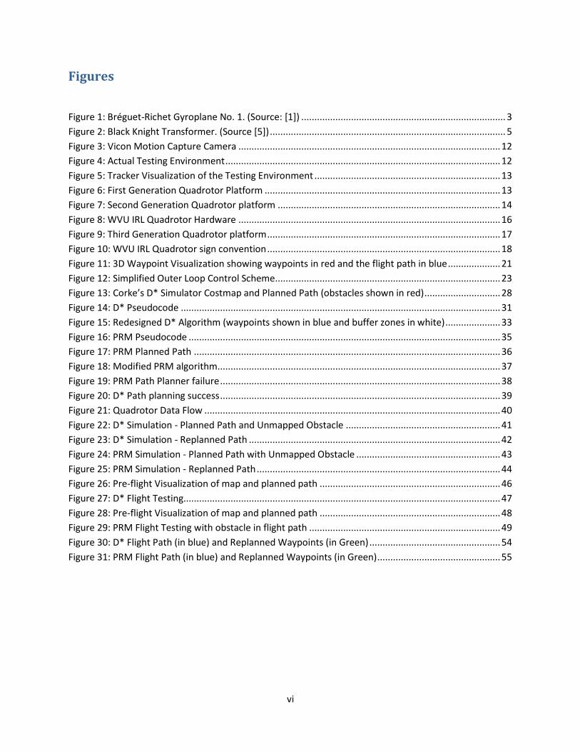
Figures
Figure 1: Bréguet-Richet Gyroplane No. 1. (Source: [1]) .............................................................................. 3
Figure 2: Black Knight Transformer. (Source [5]) .......................................................................................... 5
Figure 3: Vicon Motion Capture Camera .................................................................................................... 12
Figure 4: Actual Testing Environment ......................................................................................................... 12
Figure 5: Tracker Visualization of the Testing Environment ....................................................................... 13
Figure 6: First Generation Quadrotor Platform .......................................................................................... 13
Figure 7: Second Generation Quadrotor platform ..................................................................................... 14
Figure 8: WVU IRL Quadrotor Hardware .................................................................................................... 16
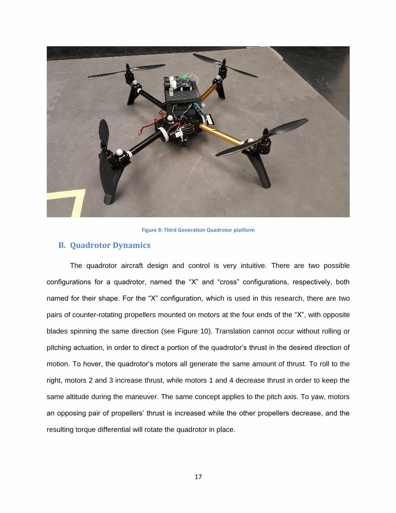
Figure 9: Third Generation Quadrotor platform ......................................................................................... 17
Figure 10: WVU IRL Quadrotor sign convention ......................................................................................... 18
Figure 11: 3D Waypoint Visualization showing waypoints in red and the flight path in blue .................... 21
Figure 12: Simplified Outer Loop Control Scheme...................................................................................... 23
Figure 13: Corke’s D* Simulator Costmap and Planned Path (obstacles shown in red) ............................. 28
Figure 14: D* Pseudocode .......................................................................................................................... 31
Figure 15: Redesigned D* Algorithm (waypoints shown in blue and buffer zones in white) ..................... 33
Figure 16: PRM Pseudocode ....................................................................................................................... 35
Figure 17: PRM Planned Path ..................................................................................................................... 36
Figure 18: Modified PRM algorithm............................................................................................................ 37
Figure 19: PRM Path Planner failure ........................................................................................................... 38
Figure 20: D* Path planning success ........................................................................................................... 39
Figure 21: Quadrotor Data Flow ................................................................................................................. 40
Figure 22: D* Simulation - Planned Path and Unmapped Obstacle ........................................................... 41
Figure 23: D* Simulation - Replanned Path ................................................................................................ 42
Figure 24: PRM Simulation - Planned Path with Unmapped Obstacle ....................................................... 43
Figure 25: PRM Simulation - Replanned Path ............................................................................................. 44
Figure 26: Pre-flight Visualization of map and planned path ..................................................................... 46
Figure 27: D* Flight Testing......................................................................................................................... 47
Figure 28: Pre-flight Visualization of map and planned path ..................................................................... 48
Figure 29: PRM Flight Testing with obstacle in flight path ......................................................................... 49
Figure 30: D* Flight Path (in blue) and Replanned Waypoints (in Green) .................................................. 54
Figure 31: PRM Flight Path (in blue) and Replanned Waypoints (in Green) ............................................... 55
vii
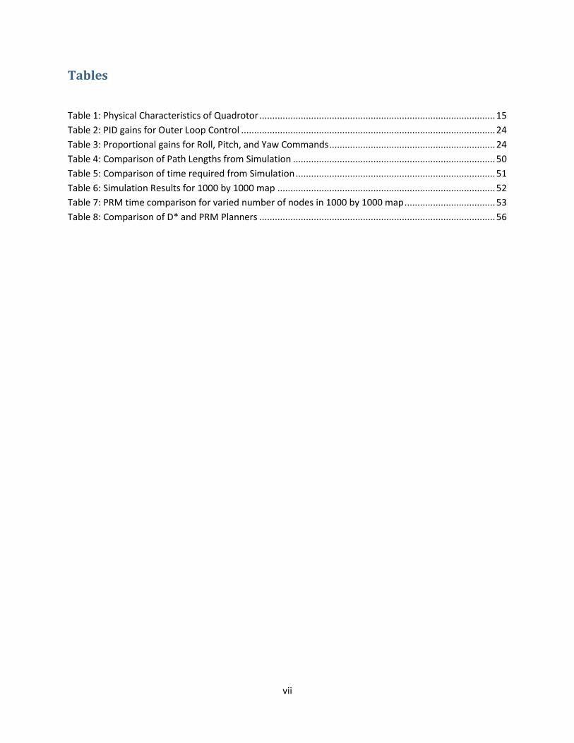
Tables
Table 1: Physical Characteristics of Quadrotor ........................................................................................... 15
Table 2: PID gains for Outer Loop Control .................................................................................................. 24
Table 3: Proportional gains for Roll, Pitch, and Yaw Commands ................................................................ 24
Table 4: Comparison of Path Lengths from Simulation .............................................................................. 50
Table 5: Comparison of time required from Simulation ............................................................................. 51
Table 6: Simulation Results for 1000 by 1000 map .................................................................................... 52
Table 7: PRM time comparison for varied number of nodes in 1000 by 1000 map ................................... 53
Table 8: Comparison of D* and PRM Planners ........................................................................................... 56
1
I. Introduction
A. Background
The quadrotor -or quadcopter- aircraft design is a novel vertical takeoff aircraft that is
rapidly gaining a foothold in the aircraft research and hobbyist communities. This class of
aircraft has numerous advantages that make it an ideal platform for airborne research. A few of
these benefits include no control linkages for reduced complexity, inexpensive and readily
available parts, battery power for cost efficient energy consumption, as well as vertical takeoff,
small size and extreme maneuverability. This has become one of the most widespread flight
vehicles used in academia.
Many quadrotors are outfitted with expensive equipment for sensing, navigation, or
surveillance. Many are made completely autonomous, extending their applications so that they
are not limited by control transmission distance from a human operator. The modification of
these aircraft for autonomous flight yields the problems of control and navigation. The desire to
traverse from one point to another without damaging the vehicle or its payload necessitates
map-based path planning to allow avoidance of obstacles. This is further complicated in real-life
scenarios when a map is not completely accurate or the mapped area changes. To meet these
needs, a number of replanning algorithms have been created. There are often several variations
on each algorithm, and many are case dependent. Real world applicability is severely limited if a
quadrotor cannot reliably navigate through such a setting.
Though their uses are varied, it is only when these vehicles are capable of completely
independent operation that they live up to their full potential. Therefore, the motivation of this
work is to ensure that a quadrotor aircraft can autonomously navigate an inaccurately mapped
or dynamic environment in a safe and reliable manner without the intervention of a human
operator.
2
B. Problem Statement and Objectives
The goal of the research presented in this report is to design, build, and operate a
Vertical Takeoff and Landing (VTOL) quadrotor Unmanned Aerial Vehicle (UAV) that is able to
navigate through an indoor environment simulating outdoor conditions, such as a forest, while
avoiding unmapped obstacles encountered along the path in real time using a map-based path
planning algorithm. The objectives are as follows:
Two map based path planning algorithms, D* and Probabilistic Roadmap method,
will be integrated and tested on the quadrotor test bed.
The performance of these algorithms will be analyzed and compared in order to
determine the most appropriate method for object avoidance in a cluttered
environment.
C. Report Structure
The second chapter is a literature review of research relevant to this topic. The third
chapter is a technical discussion of the development and structure of the quadrotor aircraft as
well as the algorithms to be implemented. The fourth chapter describes the simulation and flight
testing procedures used in analysis of the algorithms on the quadrotor test bed. The fifth chapter
summarizes the results, and the sixth chapter summarizes and concludes the paper with future
work.
3
II. Literature Review
A. The Quadrotor
1. Historical Background
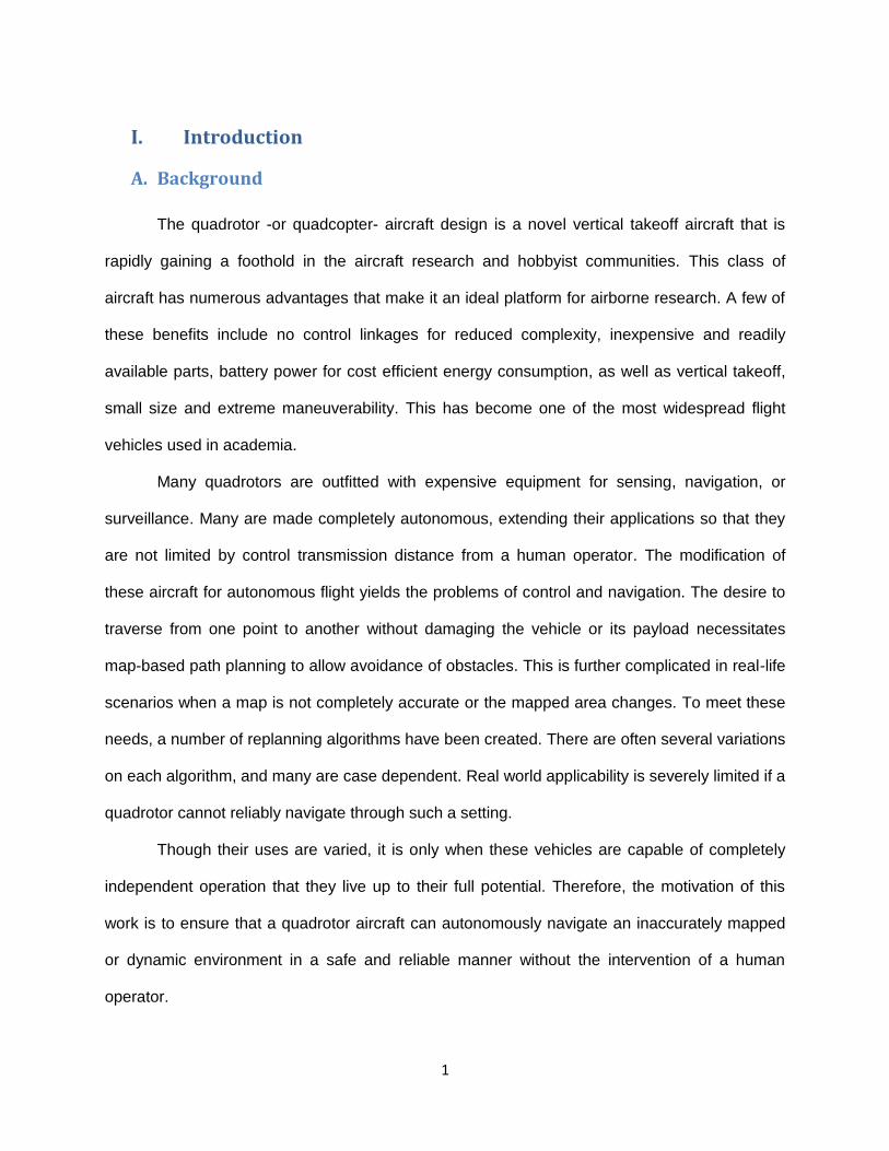
Despite the recent trend of utilizing the quadrotor aircraft in a variety of applications, this
platform is not a new idea. Some of the first aircraft were based on quadrotor designs. The very
first quadrotor design ever implemented was in 1907 when French aviation pioneer Louis
Bréguet and his brother Jacques, inspired by scientist Charles Richet, built their Bréguet-Richet
Gyroplane No. 1 (see Figure 1). This vehicle was a set of four steel-tube girders arranged in a
cross with propellers at the four ends of the cross. Each propeller was 8.1m in diameter and had
four fabric covered biplane surfaces for a total of 32 surfaces to provide thrust. It used an 8
cylinder engine, and weighed approximately 1,200lbs or more at takeoff. The primary problem
with it was that stability was quite poor and as a result was tethered, and the pilot only had
control of the throttle of the engine [1].
Figure 1: Bréguet-Richet Gyroplane No. 1. (Source: [1])
Over a decade later in 1922, another vertical takeoff aircraft began flying. Built by
another Frenchman, Etienne Oehmichen, the Oehmichen No. 2 followed a similar design with
four rotors at the ends of a cross. However, for lateral stability Oehmichen used five small
horizontal propellers, two more for forward thrust, and a final propeller for steering. The
Oehmichen was able to remain airborne for several minutes and established several records at
4
the time including the first closed circuit flight of 1km by a rotary wing vehicle. Ultimately
however, complexity and impracticalities plagued this pioneering machine [2].
There were several other attempts, but as conventional aircraft became more popular
little was done with the quadrotor design over the next couple of decades. However, in the mid
1950’s a new design was built and tested. The Convertawings Model A Quadrotor, built by Marc
Kaplan, was the first true quadrotor. Utilizing only four rotors, the Model A weighed 1 ton and
utilized two 90 hp engines. Instead of using another propeller for forward thrust, it varied the
thrust of the four main rotors instead, creating moments around the center of gravity that were
used for control. While this design was largely successful, fixed wing aircraft were preferred in
nearly every category such as range and speed, in addition to the fact that the pilot’s workload
was much lighter [3].
2. Manned and Military applications
There have been a few attempts in recent years to make full-scale manned multirotor
aircraft, but they are not very common due to numerous technical difficulties. Electric propulsion
was usually not powerful enough, and typical combustion engines cannot change RPM fast
enough to be practical for full size quadrotor applications [4]. Engine failure on a manned flight
might also be catastrophic. However, there are several companies that are pushing these
boundaries with variations on the quadrotor design. The first is Advanced Tactics and their
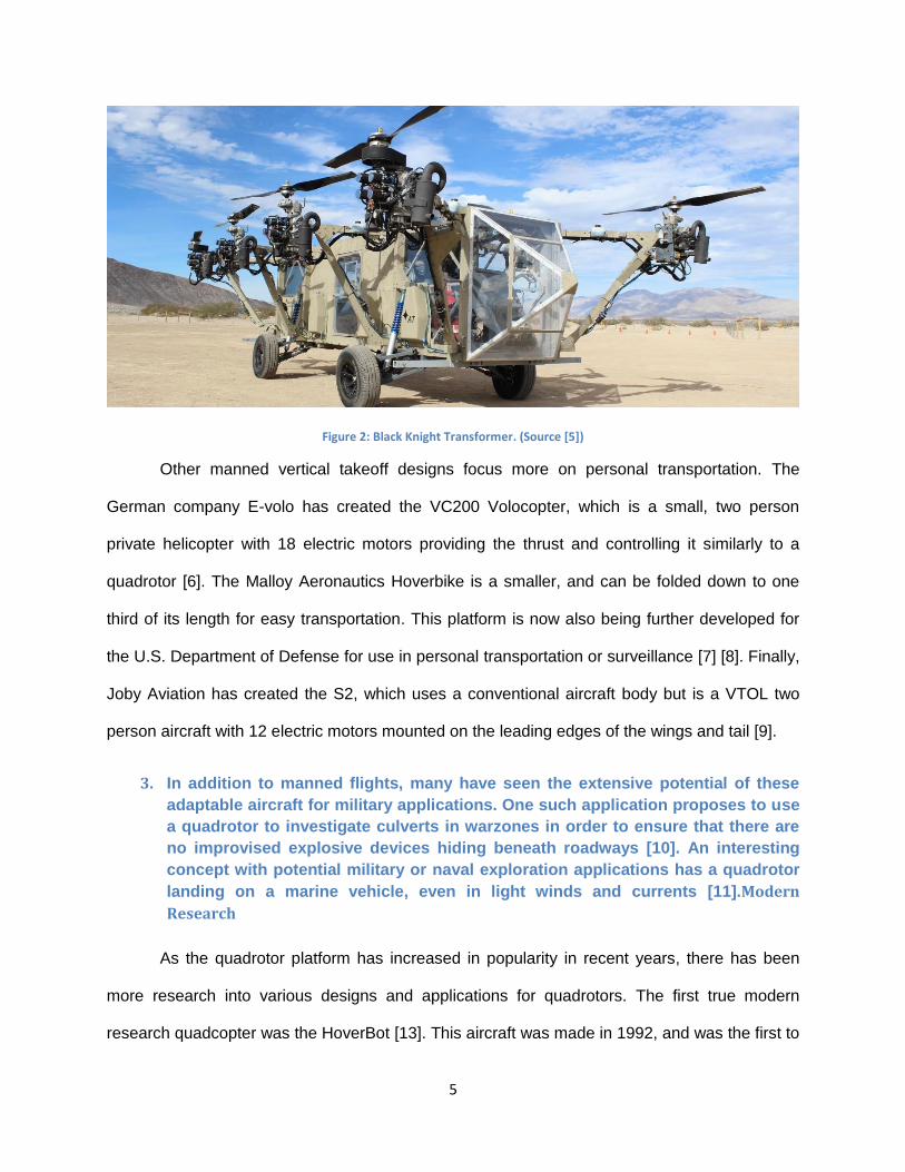
Black Knight Transformer aircraft which employs eight engines instead of four (see Figure 2). It
can travel on the ground or through the air, and is designed to be a cargo or medivac transport
vehicle more flexible than its counterparts [5].
5
Figure 2: Black Knight Transformer. (Source [5])
Other manned vertical takeoff designs focus more on personal transportation. The
German company E-volo has created the VC200 Volocopter, which is a small, two person
private helicopter with 18 electric motors providing the thrust and controlling it similarly to a
quadrotor [6]. The Malloy Aeronautics Hoverbike is a smaller, and can be folded down to one
third of its length for easy transportation. This platform is now also being further developed for
the U.S. Department of Defense for use in personal transportation or surveillance [7] [8]. Finally,
Joby Aviation has created the S2, which uses a conventional aircraft body but is a VTOL two
person aircraft with 12 electric motors mounted on the leading edges of the wings and tail [9].
3. In addition to manned flights, many have seen the extensive potential of these
adaptable aircraft for military applications. One such application proposes to use
a quadrotor to investigate culverts in warzones in order to ensure that there are
no improvised explosive devices hiding beneath roadways [10]. An interesting
concept with potential military or naval exploration applications has a quadrotor
landing on a marine vehicle, even in light winds and currents [11].Modern
Research
As the quadrotor platform has increased in popularity in recent years, there has been
more research into various designs and applications for quadrotors. The first true modern
research quadcopter was the HoverBot [13]. This aircraft was made in 1992, and was the first to
6
overcome the inherent instability of small-sized helicopters using onboard computing and
electronic power. At that time, electronics were just becoming small and powerful enough to fit
such an application, and batteries were beginning to have larger power-to-weight ratios.
However a typical Remote Controlled (RC) helicopter could not produce the required power to
support the extra weight from the electronics. Thus the quadrotor design was chosen, and
essentially implemented as four helicopters linked by the tails. Their design allowed for tethered
indoor flight, another first for the quadrotor. Despite the modest results, this was a large step
forward in the evolution of modern quadcopters.
Since that time, many other fascinating projects utilizing the flexibility of the quadrotor
have embodied themselves, often related to surveillance. Since flight times are still relatively
short however, a major area of study is extending the duration of surveillance missions to
increase effectiveness. A common way to achieve this is to “perch-and-stare,” where the
quadrotor lands on a suitable surface to save battery power while a camera continues
surveillance. One group has built a quadrotor that can perch on a large variety of surfaces while
using almost no power by utilizing a bio-mimetic mechanism [19]. In addition to vertical landing,
actuators may also be used to expand a quadrotor’s capabilities to interact with the environment
in other ways, to pick up other objects or even perch upside down [21]. While this is potentially
very useful, a quadrotor equipped with such an actuator still needs to be controlled precisely to
be able to utilize this. To achieve this, the University of Pennsylvania’s GRASP lab has
developed an algorithm which allows a quadrotor to perch on an arbitrarily oriented line [20].
Another research aircraft that could be useful for such surveillance applications is the SquidCop.
This quadcopter aims to increase the flight time it can maintain at its mission site, and achieves
this by deploying from a fixed wing carrier aircraft at low speeds. This allows the quadrotor to
use little or no power reaching the surveillance point [12].
Another very popular research topic with quadrotor aircraft is cooperative swarms which
can achieve much more than a single aircraft. With this trend comes the need for simple, low
7
cost platforms to facilitate large numbers of quadrotors flying concurrently. Electronics are
constantly becoming cheaper and more readily available, building swarms of quadrotors and
equipping them with electronics and sensors possible [27]. Many algorithms have been made to
control swarms of autonomous vehicles using coordinated formations, path planning and object
avoidance procedures [28] [29] [30] [31] [32]. These capabilities can be used for surveillance
patrols or other applications where numerous vehicles are in close operational proximity to each
other. Some have even extended the use of these swarms to perform tasks in areas dangerous
to humans. Penn’s GRASP lab and the Technological Institute of Aeronautics in Brazil both
have attached grippers to their quadrotors to assemble a variety of geometric truss structures
using special assembly members in a construction scenario [33] [34]. Another hazardous
application for swarms includes mass deployment in disaster zones for expanding
telecommunication and WiFi signals [35].
There are several other more creative cooperative applications for quadrotors that have
been investigated and implemented at ETH Zurich in Switzerland. They include carrying a large
flexible payload similar to a hula hoop [36], throwing and catching a ball using a net [37], and
even execute aerial dance choreography in time with music [38]. Control can also be achieved
using a Microsoft Kinect sensor to directly interact with the quadrotor simply using motions [39].
Additionally, they have experimented with a modular, single propeller robot that can
autonomously drive around the room, dock with other robots, and fly in a coordinated fashion
while connected. [40]
B. Path planning and Control
1. Dijkstra’s Algorithm
One of the foundational modern map-based planning algorithms is Dijkstra’s Algorithm,
published in 1959. Named after its Dutch creator, this algorithm solves the problem of the
shortest total length between a start and goal node given the lengths of all branches that
8
connect the nodes. It can also be used to find the shortest path from the start node to all other
nodes. It takes into account only the neighboring nodes and then moves from the current point
to the next “best” point. It will not return to any node it has already visited and will continue until
the destination is reached [41]. It is very efficient since each iteration of the algorithm only relies
on previously determined information. Due to its efficiency it is one of the most widely used
methods for finding the shortest path in a digraph [42].
This algorithm has obvious uses in robotics and path planning for autonomous vehicles
[43] [44], but it has also been used in a variety of other interesting applications through the
years. One group discusses using a modified version to route emergency vehicles in natural
disaster areas [45], and another uses it for airline network planning [46]. Dijkstra’s algorithm has
even been utilized to evaluate a 3D skeletonization of the brain’s vascular network [47].
Despite its advantages, Dijkstra’s Algorithm is very hard to parallelize, or run
concurrently on multiple devices for increased speed. Some work has been done to parallelize it
using transactional memory and helper threading, which shows some moderate improvements
to the basic serial algorithm [48] [49]. Others have made improvements to the algorithm by
considering node weights in addition to the edge weights [50], or improving its storage structure
and search area [51]. Some go as far to argue that Dijkstra’s Algorithm should not be used at all
any more, replacing it with the Uniform-Cost Search method which is very similar but superior to
Dijkstra’s Algorithm [52].
2. A*
In 1967 another important algorithm was made called A* (pronounced “A-Star”) which
improved upon Dijkstra’s Algorithm by using heuristics to weight the search towards the goal
node. This algorithm is admissible, meaning it is guaranteed to find an optimal path to the goal
node, and will process the fewest nodes necessary to find the optimal path [53]. There are many
similar applications of A*, thus it has been compared to Dijkstra’s Algorithm frequently [54].
9
Though it generally achieves good results, the complexity can be a drawback for larger
maps. As a result, there have been several improvement or variations off of the A* algorithm as
well [55] [56]. One of these is called Ae, which is not admissible but, rather than seeking an
optimal solution, will look for one that is close to optimum. The idea is that increased
computational efficiency may be achieved at the cost of a bounded loss in optimality [57].
Another adapts A* for use in areas where a “large” map is necessary, reducing the necessary
processing resources [58].
3. D*
Another major map based planning algorithm in history is based off of A*. Created by
Anthony Stentz in 1994, Dynamic A*, or simply D*, extends A* planning to include replanning in
unknown or changing environments while retaining optimality and efficiency. It can handle any
amount of map information from none at all to a complete and accurate map [59]. Stentz also
made several variations on his algorithm. The first of these is the Focussed D* algorithm which
reduces the time needed for path planning and replanning. After the initial plan, the algorithm
then changes the path as needed during the execution of the plan, still following an optimal path
at every step [60]. Another D* algorithm modification was made by Koenig and Likhachev, who
called their new algorithm D* Lite. D* Lite is essentially the same algorithm as Focussed D* but
is easier to understand and more efficient [61]. After these changes, another modification was
made by Stentz to the algorithm, this time called Delayed D*. This algorithm is simply more
efficient in how it modifies the map during the mission making it superior to even D* Lite [62].
Stentz et al also worked to combine D*’s incremental replanning with an anytime algorithm, or
one that will calculate the best solution within the available time since generating an optimal
solution may not be feasible. The result is known as Anytime Dynamic A*, which takes the best
qualities form both types of planners to give solutions to complex and changing environments
[63].
10
The D* family of algorithms is used across a spectrum of applications, ranging from an
enhanced version of the basic algorithm for basic ground robot navigation in indoor
environments [64] to simulating flights of unmanned combat aircraft [65]. They also can be
integrated with other algorithms to provide practical improvements such as reactive collision
avoidance in addition to path planning [66] or to smooth the path generated by D* [67].
For grid based algorithms such as A* and D*, the generated path is optimal. However
optimality is only guaranteed to be as good as the grid resolution of the map, and as the grid
grows run-time increases exponentially [68]. This problem may potentially be remedied by using
different methods, particularly roadmap methods.
4. Probabilistic Roadmap Method
One of these algorithms is named the Probabilistic Roadmap method, or PRM, which is
part of the sampling-based roadmap family of algorithms. This method is built for motion
planning for holonomic robots – robots that may move in any direction – in static spaces, and is
easy to understand and implement. It has two phases: the learning phase in which the map is
built, and the query phase in which the path through the map is planned. In the learning phase,
points are chosen at random and set as nodes. Edges are then added between these nodes to
denote they are passable, which is termed “local planning” [69]. In the query phase a path is
chosen between the nodes. Occasionally this is achieved using Dijkstra’s algorithm [70], [71],
[72], [73], but can be through other methods as well.
One of the major drawbacks to PRM’s is the fact that they often will not perform well in
narrow passages, sometimes not even arriving at a navigation solution if node selection is
inadequate. Modifications have been made to the learning phase of the planner to take into
account these locations and ensure proper sampling in these areas [72], [73], [74], [75]. One
method even allows several learning techniques to be stored, and chooses the correct one for a
given application [76].
11
The PRM method has been used for trajectory generation in three dimensions for aircraft
[77], multiple robot configurations [78], as well as other general mobile platforms [71]. One
technique alters the generated nodes in order to create more practical, less random paths [79].
Another attempts to parallelize the PRM method [80]. Work has even been done to allow PRM’s
to take into account roadmap inaccuracies by adding a probability of collision to the edges and
nodes [70].
The PRM algorithm is known to be suboptimal, due to the random nature of the node
selection. However, there are several alternative methods based on the PRM algorithm that
provide optimality. Some of these also retain very good computational efficiency [68] which may
make these methods a viable alternative to grid based planning algorithms.
12
III. Technical Discussion
A. Testbed and Testing Environment
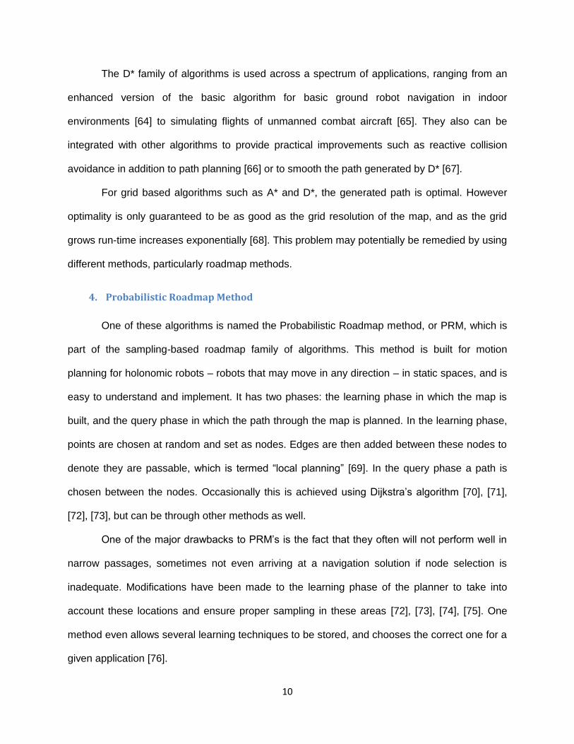
The West Virginia University Interactive
Robotics Laboratory outfitted an indoor flight
testing facility specifically for quadrotor UAVs. The
testing area is roughly a 4x4x2m room with anti-
reflective paint and a foam ground mat. Safety
equipment includes sprinkler guards and a safety
net to provide protection to the room, the pilot, and bystanders during indoor quadrotor flight
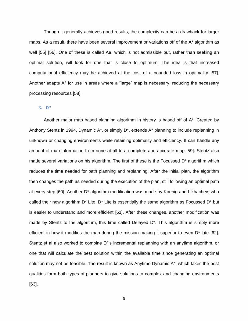
testing. A Vicon infrared motion capture camera system (see Figure 3) was installed along with
Vicon’s Tracker software. This system allows real-time millimeter accuracy three-dimensional
position tracking of multiple objects at a high frequency through tracking infrared reflective
spheres attached to the subject(s) of interest. A unique orientation of the reflectors is required to
define an object to the Tracker software so that it may differentiate between the objects in the
workspace (see Figure 4 and Figure 5). In addition, Quarc Real-Time control software is utilized
with MATLAB and Simulink in conjunction with Tracker to allow real-time collection and analysis
of Vicon position data on a ground station computer.
Figure 4: Actual Testing Environment
Figure 3: Vicon Motion Capture Camera
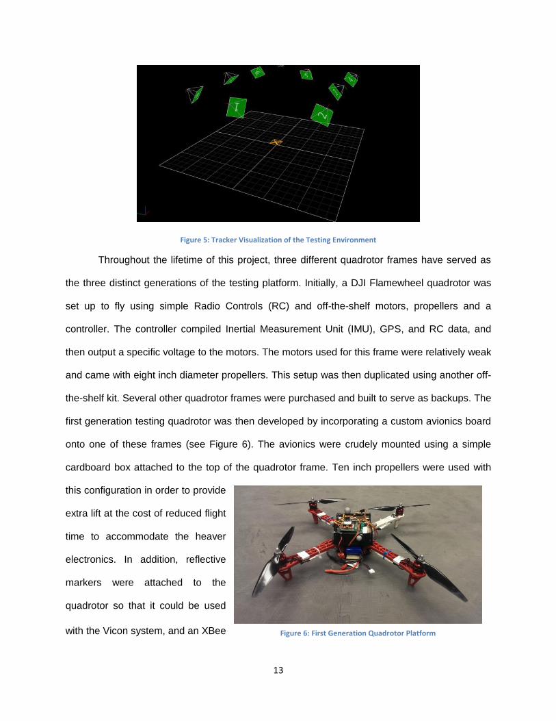
13
Figure 5: Tracker Visualization of the Testing Environment
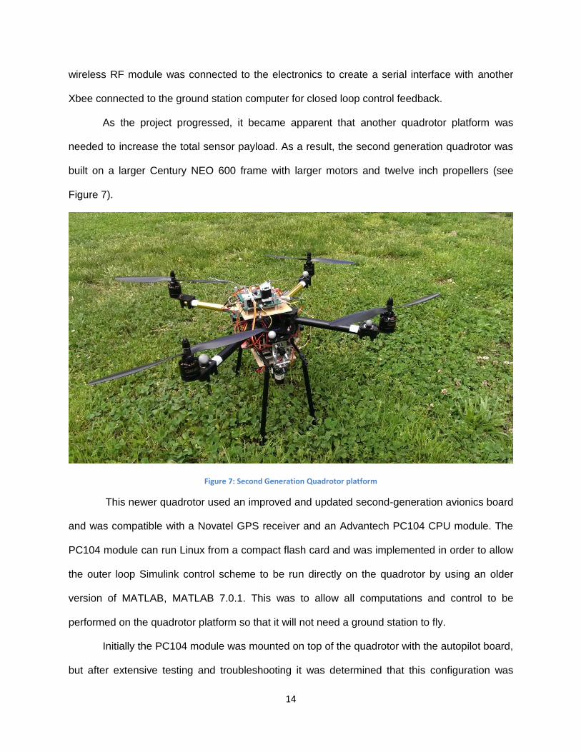
Throughout the lifetime of this project, three different quadrotor frames have served as
the three distinct generations of the testing platform. Initially, a DJI Flamewheel quadrotor was
set up to fly using simple Radio Controls (RC) and off-the-shelf motors, propellers and a
controller. The controller compiled Inertial Measurement Unit (IMU), GPS, and RC data, and
then output a specific voltage to the motors. The motors used for this frame were relatively weak
and came with eight inch diameter propellers. This setup was then duplicated using another off-
the-shelf kit. Several other quadrotor frames were purchased and built to serve as backups. The
first generation testing quadrotor was then developed by incorporating a custom avionics board
onto one of these frames (see Figure 6). The avionics were crudely mounted using a simple
cardboard box attached to the top of the quadrotor frame. Ten inch propellers were used with
this configuration in order to provide
extra lift at the cost of reduced flight
time to accommodate the heaver
electronics. In addition, reflective
markers were attached to the
quadrotor so that it could be used
with the Vicon system, and an XBee Figure 6: First Generation Quadrotor Platform
14
wireless RF module was connected to the electronics to create a serial interface with another
Xbee connected to the ground station computer for closed loop control feedback.
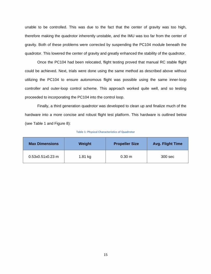
As the project progressed, it became apparent that another quadrotor platform was
needed to increase the total sensor payload. As a result, the second generation quadrotor was
built on a larger Century NEO 600 frame with larger motors and twelve inch propellers (see
Figure 7).
Figure 7: Second Generation Quadrotor platform
This newer quadrotor used an improved and updated second-generation avionics board
and was compatible with a Novatel GPS receiver and an Advantech PC104 CPU module. The
PC104 module can run Linux from a compact flash card and was implemented in order to allow
the outer loop Simulink control scheme to be run directly on the quadrotor by using an older
version of MATLAB, MATLAB 7.0.1. This was to allow all computations and control to be
performed on the quadrotor platform so that it will not need a ground station to fly.
Initially the PC104 module was mounted on top of the quadrotor with the autopilot board,
but after extensive testing and troubleshooting it was determined that this configuration was
15
unable to be controlled. This was due to the fact that the center of gravity was too high,
therefore making the quadrotor inherently unstable, and the IMU was too far from the center of
gravity. Both of these problems were corrected by suspending the PC104 module beneath the
quadrotor. This lowered the center of gravity and greatly enhanced the stability of the quadrotor.
Once the PC104 had been relocated, flight testing proved that manual RC stable flight
could be achieved. Next, trials were done using the same method as described above without
utilizing the PC104 to ensure autonomous flight was possible using the same inner-loop
controller and outer-loop control scheme. This approach worked quite well, and so testing
proceeded to incorporating the PC104 into the control loop.
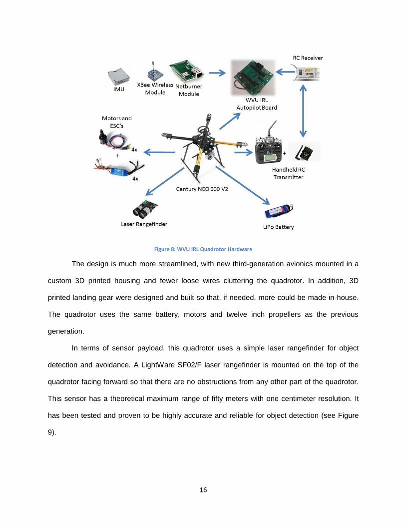
Finally, a third generation quadrotor was developed to clean up and finalize much of the
hardware into a more concise and robust flight test platform. This hardware is outlined below
(see Table 1 and Figure 8):
Table 1: Physical Characteristics of Quadrotor
Max Dimensions Weight Propeller Size Avg. Flight Time
0.53x0.51x0.23 m 1.81 kg 0.30 m 300 sec
16
Figure 8: WVU IRL Quadrotor Hardware
The design is much more streamlined, with new third-generation avionics mounted in a
custom 3D printed housing and fewer loose wires cluttering the quadrotor. In addition, 3D
printed landing gear were designed and built so that, if needed, more could be made in-house.
The quadrotor uses the same battery, motors and twelve inch propellers as the previous
generation.
In terms of sensor payload, this quadrotor uses a simple laser rangefinder for object
detection and avoidance. A LightWare SF02/F laser rangefinder is mounted on the top of the
quadrotor facing forward so that there are no obstructions from any other part of the quadrotor.
This sensor has a theoretical maximum range of fifty meters with one centimeter resolution. It
has been tested and proven to be highly accurate and reliable for object detection (see Figure
9).
17
Figure 9: Third Generation Quadrotor platform
B. Quadrotor Dynamics
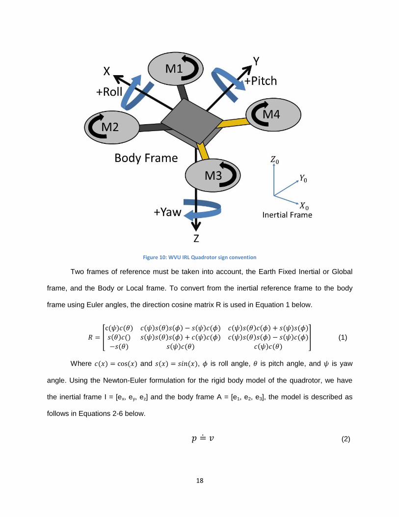
The quadrotor aircraft design and control is very intuitive. There are two possible
configurations for a quadrotor, named the “X” and “cross” configurations, respectively, both
named for their shape. For the “X” configuration, which is used in this research, there are two
pairs of counter-rotating propellers mounted on motors at the four ends of the “X”, with opposite
blades spinning the same direction (see Figure 10). Translation cannot occur without rolling or
pitching actuation, in order to direct a portion of the quadrotor’s thrust in the desired direction of
motion. To hover, the quadrotor’s motors all generate the same amount of thrust. To roll to the
right, motors 2 and 3 increase thrust, while motors 1 and 4 decrease thrust in order to keep the
same altitude during the maneuver. The same concept applies to the pitch axis. To yaw, motors
an opposing pair of propellers’ thrust is increased while the other propellers decrease, and the
resulting torque differential will rotate the quadrotor in place.
18
Figure 10: WVU IRL Quadrotor sign convention
Two frames of reference must be taken into account, the Earth Fixed Inertial or Global
frame, and the Body or Local frame. To convert from the inertial reference frame to the body
frame using Euler angles, the direction cosine matrix R is used in Equation 1 below.
𝑅 = [
c(𝜓)𝑐(𝜃) 𝑐(𝜓)𝑠(𝜃)𝑠(𝜙) − 𝑠(𝜓)𝑐(𝜙) 𝑐(𝜓)𝑠(𝜃)𝑐(𝜙) + 𝑠(𝜓)𝑠(𝜙)
𝑠(𝜃)𝑐() 𝑠(𝜓)𝑠(𝜃)𝑠(𝜙) + 𝑐(𝜓)𝑐(𝜙) 𝑐(𝜓)𝑠(𝜃)𝑠(𝜙) − 𝑠(𝜓)𝑐(𝜙)
−𝑠(𝜃) 𝑠(𝜓)𝑐(𝜃) 𝑐(𝜓)𝑐(𝜃)] (1)
Where 𝑐(𝑥) = cos(𝑥) and 𝑠(𝑥) = 𝑠𝑖𝑛(𝑥), 𝜙 is roll angle, 𝜃 is pitch angle, and 𝜓 is yaw
angle. Using the Newton-Euler formulation for the rigid body model of the quadrotor, we have
the inertial frame I = [ex, ey, ez] and the body frame A = [e1, e2, e3], the model is described as
follows in Equations 2-6 below.
𝑝 = 𝑣̇ (2)
19
�̇� = 𝑔𝑒𝑧 −
1
𝑚𝑇𝑅𝑒𝑧 (3)
�̇� = 𝑅𝑆(𝛺) (4)
𝐼𝑓�̇� = −𝛺 × 𝐼𝑓𝛺 − 𝐺𝑎 + 𝜏𝑎 (5)
𝐼𝑟�̇�𝑖 = 𝜏𝑖 − 𝑄𝑖 ,𝑖 ∈ {1,2,3,4} (6)
Where p is the x, y, z origin positon of the body frame with respect to the inertial frame, v
is the velocity of the origin of the body frame, g is acceleration due to gravity, m is mass of the
quadrotor. For the vector Ω = (Ω1, Ω2, Ω3)T S(Ω) is the skew-symmetric matrix defined in
Equation 7 below.
𝑆(𝛺) = [
0 −𝛺3 𝛺2
𝛺3 0 −𝛺1−𝛺2 𝛺1 0
] (7)
Torque 𝑄 is generated due to the drag forces of each of the rotors acting on the air. This
is modeled by Equation 8:
𝑄𝑖 = 𝜅𝜔𝑖2
(8)
Thrust 𝑇 is the sum of the thrust from all motors, shown with Equation 9.
𝑇 = 𝑏∑𝜔𝑖2
4
𝑖=1
(9)
Where 𝜅 and 𝑏 are coefficients varying with propeller shape, pitch, size, etc. Gyroscopic
torque from airframe and rotor rotation is given by:
𝐺𝑎 =∑𝐼𝑟(𝛺 × 𝑒𝑧)(−1)𝑖+1𝜔𝑖
4
𝑖=1
(10)
The airframe torque 𝜏𝑎 due to the rotors are from the following equations:
20
𝜏𝑎1 = 𝑑𝑏(𝜔2
2 −𝜔42)
𝜏𝑎2 = 𝑑𝑏(𝜔1
2 −𝜔22)
𝜏𝑎3 = 𝜅(𝜔1
2 +𝜔32 −𝜔2
2 −𝜔42)
(11)
Where d is the length from the origin of the body frame at the center of mass of the
quadrotor to the rotor. These can be combined as shown below in Equation 12.
𝜏𝑎 = [
𝜏𝑎1
𝜏𝑎2
𝜏𝑎3
] (12)
Lastly, the torque produced by a given rotor is denoted by 𝜏𝑖 [81].
C. Software
1. Outer Loop Control
An outer loop control scheme was designed in Simulink to be run on the ground station
computer using feedback from the Vicon system and Quarc software to control the quadrotor.
The basic scheme applied with this system is a simple waypoint navigation controller. It employs
a Matlab script to initialize desired position, which generates a user-friendly Graphical User
Interface (GUI) that guides the user in choosing waypoints around the test area in three-
dimensional space. An imaginary sphere of a specific radius is then placed around those points.
The final set of waypoints and spheres can be viewed in 3D with a ground trace for enhanced
perspective. These waypoints are then output as a matrix of xyz coordinates into Simulink.
Simulink will control the quadrotor as described above using a constant yaw angle and the first
waypoint’s xyz coordinates as the current desired location. When the quadrotor enters any part
of the sphere around the waypoint, the control scheme then accepts that the waypoint was
reached and updates the desired location to the next waypoint, and so on. When the last
waypoint is reached then the next waypoint loops back to be the initial waypoint so that flight is
21
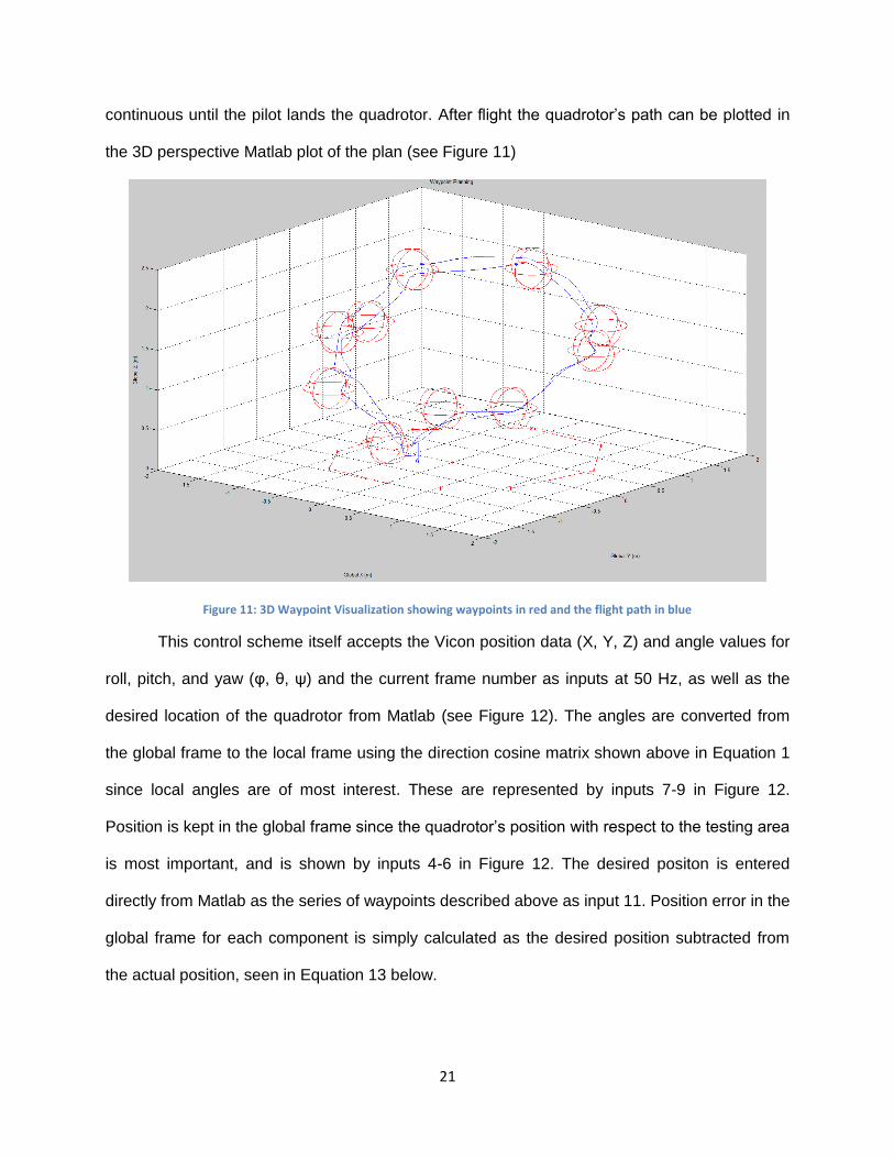
continuous until the pilot lands the quadrotor. After flight the quadrotor’s path can be plotted in
the 3D perspective Matlab plot of the plan (see Figure 11)
Figure 11: 3D Waypoint Visualization showing waypoints in red and the flight path in blue
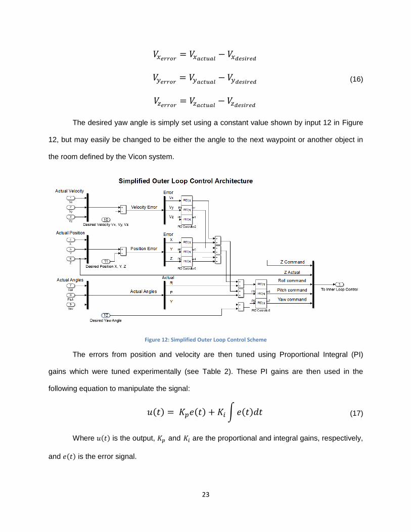
This control scheme itself accepts the Vicon position data (X, Y, Z) and angle values for
roll, pitch, and yaw (φ, θ, ψ) and the current frame number as inputs at 50 Hz, as well as the
desired location of the quadrotor from Matlab (see Figure 12). The angles are converted from
the global frame to the local frame using the direction cosine matrix shown above in Equation 1
since local angles are of most interest. These are represented by inputs 7-9 in Figure 12.
Position is kept in the global frame since the quadrotor’s position with respect to the testing area
is most important, and is shown by inputs 4-6 in Figure 12. The desired positon is entered
directly from Matlab as the series of waypoints described above as input 11. Position error in the
global frame for each component is simply calculated as the desired position subtracted from
the actual position, seen in Equation 13 below.
22
𝑥𝑒𝑟𝑟𝑜𝑟 = 𝑥𝑎𝑐𝑡𝑢𝑎𝑙 − 𝑥𝑑𝑒𝑠𝑖𝑟𝑒𝑑
𝑦𝑒𝑟𝑟𝑜𝑟 = 𝑦𝑎𝑐𝑡𝑢𝑎𝑙 − 𝑦𝑑𝑒𝑠𝑖𝑟𝑒𝑑
𝑧𝑒𝑟𝑟𝑜𝑟 = 𝑧𝑎𝑐𝑡𝑢𝑎𝑙 − 𝑧𝑑𝑒𝑠𝑖𝑟𝑒𝑑
(13)
The velocity is calculated from the position and current time step information directly
from Vicon, and converted into the local frame as shown by Figure 12 inputs 1-3. The desired
velocity components are calculated by setting a desired total velocity and multiplying that with
the desired unit vector in each direction which is calculated from the position error. The unit
vectors are reflected in the equations below.
𝑈𝑥 = −
𝑥𝑒𝑟𝑟𝑜𝑟
√𝑥𝑒𝑟𝑟𝑜𝑟2 + 𝑦𝑒𝑟𝑟𝑜𝑟
2 + 𝑧𝑒𝑟𝑟𝑜𝑟2
𝑈𝑦 = −𝑦𝑒𝑟𝑟𝑜𝑟
√𝑥𝑒𝑟𝑟𝑜𝑟2 + 𝑦𝑒𝑟𝑟𝑜𝑟
2 + 𝑧𝑒𝑟𝑟𝑜𝑟2
𝑈𝑧 = −𝑧𝑒𝑟𝑟𝑜𝑟
√𝑥𝑒𝑟𝑟𝑜𝑟2 + 𝑦𝑒𝑟𝑟𝑜𝑟
2 + 𝑧𝑒𝑟𝑟𝑜𝑟2
(14)
The resulting desired velocity components are then found using the following equations
using the method as described above.
𝑉𝑥𝑑𝑒𝑠𝑖𝑟𝑒𝑑 = 𝑉𝑡𝑜𝑡𝑎𝑙𝑑𝑒𝑠𝑖𝑟𝑒𝑑 ∗ 𝑈𝑥
𝑉𝑦𝑑𝑒𝑠𝑖𝑟𝑒𝑑 = 𝑉𝑡𝑜𝑡𝑎𝑙𝑑𝑒𝑠𝑖𝑟𝑒𝑑 ∗ 𝑈𝑦
𝑉𝑧𝑑𝑒𝑠𝑖𝑟𝑒𝑑 = 𝑉𝑡𝑜𝑡𝑎𝑙𝑑𝑒𝑠𝑖𝑟𝑒𝑑 ∗ 𝑈𝑧
(15)
These are shown in Figure 12 below by input 10. The velocity error is then simply
calculated by taking the difference between actual and desired velocity using the following
equations.
23
𝑉𝑥𝑒𝑟𝑟𝑜𝑟 = 𝑉𝑥𝑎𝑐𝑡𝑢𝑎𝑙 − 𝑉𝑥𝑑𝑒𝑠𝑖𝑟𝑒𝑑
𝑉𝑦𝑒𝑟𝑟𝑜𝑟 = 𝑉𝑦𝑎𝑐𝑡𝑢𝑎𝑙 − 𝑉𝑦𝑑𝑒𝑠𝑖𝑟𝑒𝑑
𝑉𝑧𝑒𝑟𝑟𝑜𝑟 = 𝑉𝑧𝑎𝑐𝑡𝑢𝑎𝑙 − 𝑉𝑧𝑑𝑒𝑠𝑖𝑟𝑒𝑑
(16)
The desired yaw angle is simply set using a constant value shown by input 12 in Figure
12, but may easily be changed to be either the angle to the next waypoint or another object in
the room defined by the Vicon system.
Figure 12: Simplified Outer Loop Control Scheme
The errors from position and velocity are then tuned using Proportional Integral (PI)
gains which were tuned experimentally (see Table 2). These PI gains are then used in the
following equation to manipulate the signal:
𝑢(𝑡) = 𝐾𝑝𝑒(𝑡) + 𝐾𝑖∫𝑒(𝑡)𝑑𝑡 (17)
Where 𝑢(𝑡) is the output, 𝐾𝑝 and 𝐾𝑖 are the proportional and integral gains, respectively,
and 𝑒(𝑡) is the error signal.
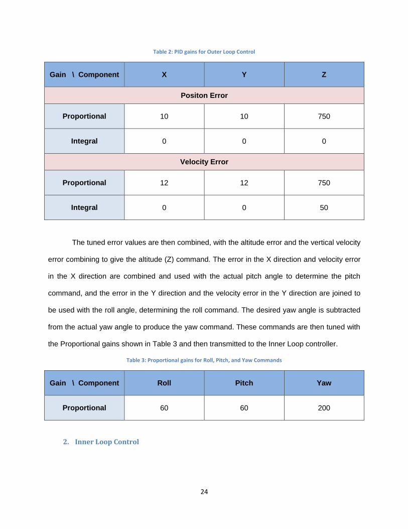
24
Table 2: PID gains for Outer Loop Control
Gain \ Component X Y Z
Positon Error
Proportional 10 10 750
Integral 0 0 0
Velocity Error
Proportional 12 12 750
Integral 0 0 50
The tuned error values are then combined, with the altitude error and the vertical velocity
error combining to give the altitude (Z) command. The error in the X direction and velocity error
in the X direction are combined and used with the actual pitch angle to determine the pitch
command, and the error in the Y direction and the velocity error in the Y direction are joined to
be used with the roll angle, determining the roll command. The desired yaw angle is subtracted
from the actual yaw angle to produce the yaw command. These commands are then tuned with
the Proportional gains shown in Table 3 and then transmitted to the Inner Loop controller.
Table 3: Proportional gains for Roll, Pitch, and Yaw Commands
Gain \ Component Roll Pitch Yaw
Proportional 60 60 200
2. Inner Loop Control
25
An Inner Loop controller was coded for a NetBurner Core Module, which interfaces with
the quadrotor’s avionics board, with the goal of achieving stable flight with a controller that could
be modified to suit a variety of desired uses. The first quadrotor was modified to use an avionics
circuit board that was designed in-house to be used with the NetBurner and an IMU instead of
the stock controller. The architecture of this Inner Loop controller essentially mimics the stock
controller with RC communication and IMU feedback. The process of testing and refining the
controller to stabilize the quadrotor using IMU feedback was carried out in phases through trial
and error. First the roll axis was tested by restricting the quadrotor’s movement by a simple
tether system, and gains were tuned until desired performance was attained. Once stable on the
roll axis, the pitch axis was tuned the same way. Finally, yaw was tuned using untethered RC
flight so that performance was nearly identical to the original controller.
Additional capabilities were added to the Inner loop, starting with a motor kill switch to
disable the motors in dangerous situations. A switch on the RC transmitter may be toggled,
which signals to the NetBurner to immediately turn off all motors. Next, auto takeoff and landing
sequences were coded into the controller to allow increased autonomy during flight. Another
switch on the transmitter is monitored by the NetBurner, and when toggled it adds to the throttle
value being sent to all motors. Also, the laser rangefinder was calibrated and integrated into the
quadrotor’s electronics. The data from the rangefinder is read by the NetBurner using analog to
digital conversion. Finally, the avionics were connected to the XBee wireless modem to allow
communication with the Outer Loop control scheme running on the ground station.
In the Inner Loop controller, commands are processed from the Outer Loop scheme, the
quadrotor’s IMU, and RC transmitter and interpreted into motor commands. As roll, pitch, and
yaw commands from the Outer Loop enter, they are processed as shown below in equations
18-20.
26
𝜙𝑐𝑜𝑛𝑡𝑟𝑜𝑙 = (𝜙𝑐𝑜𝑚𝑚𝑎𝑛𝑑) + (𝐾𝜙) ∗ (𝑒�̇�) (18)
𝜃𝑐𝑜𝑛𝑡𝑟𝑜𝑙 = (𝜃𝑐𝑜𝑚𝑚𝑎𝑛𝑑) + (𝐾𝜃) ∗ (𝑒�̇�) (19)
𝜓𝑐𝑜𝑛𝑡𝑟𝑜𝑙 = (𝜓𝑐𝑜𝑚𝑚𝑎𝑛𝑑) + (𝐾𝜓) ∗ (𝑒�̇�) (20)
Where the control variable is 𝑥𝑐𝑜𝑛𝑡𝑟𝑜𝑙, the control command from the Outer Loop
controller is 𝑥𝑐𝑜𝑚𝑚𝑎𝑛𝑑, the proportional gain is 𝐾𝑥, the IMU rate error is given by 𝑒�̇�, and x is roll
(ϕ), pitch (θ), or yaw (ψ). The roll gain is 20, pitch gain is 20 and the yaw gain is 30. The IMU
rate error is simply the rate gyro outputs from the IMU. These are denoted as errors since the
quadrotor is desired to be stable with very little or no angular motion. These control variables
are then fed into the following equations 21-24 along with the altitude (Z) command from the
Outer Loop and the pilot inputs from the RC transmitter.
𝑀1 = 𝑇𝑐𝑜𝑛𝑡𝑟𝑜𝑙 + 𝑇𝑝𝑖𝑙𝑜𝑡 + 𝜃𝑐𝑜𝑛𝑡𝑟𝑜𝑙 + 𝜃𝑝𝑖𝑙𝑜𝑡 + 𝜓𝑐𝑜𝑛𝑡𝑟𝑜𝑙 + 𝜓𝑝𝑖𝑙𝑜𝑡
− 𝜙𝑐𝑜𝑛𝑡𝑟𝑜𝑙 − 𝜙𝑝𝑖𝑙𝑜𝑡 + 𝑍𝑐𝑜𝑚𝑚𝑎𝑛𝑑 (21)
𝑀2 = 𝑇𝑐𝑜𝑛𝑡𝑟𝑜𝑙 + 𝑇𝑝𝑖𝑙𝑜𝑡 + 𝜃𝑐𝑜𝑛𝑡𝑟𝑜𝑙 + 𝜃𝑝𝑖𝑙𝑜𝑡 − 𝜓𝑐𝑜𝑛𝑡𝑟𝑜𝑙 − 𝜓𝑝𝑖𝑙𝑜𝑡
+ 𝜙𝑐𝑜𝑛𝑡𝑟𝑜𝑙 + 𝜙𝑝𝑖𝑙𝑜𝑡 + 𝑍𝑐𝑜𝑚𝑚𝑎𝑛𝑑 (22)
𝑀3 = 𝑇𝑐𝑜𝑛𝑡𝑟𝑜𝑙 + 𝑇𝑝𝑖𝑙𝑜𝑡 − 𝜃𝑐𝑜𝑛𝑡𝑟𝑜𝑙 − 𝜃𝑝𝑖𝑙𝑜𝑡 + 𝜓𝑐𝑜𝑛𝑡𝑟𝑜𝑙 + 𝜓𝑝𝑖𝑙𝑜𝑡
+ 𝜙𝑐𝑜𝑛𝑡𝑟𝑜𝑙 + 𝜙𝑝𝑖𝑙𝑜𝑡 + 𝑍𝑐𝑜𝑚𝑚𝑎𝑛𝑑
(23)
𝑀4 = 𝑇𝑐𝑜𝑛𝑡𝑟𝑜𝑙 + 𝑇𝑝𝑖𝑙𝑜𝑡 − 𝜃𝑐𝑜𝑛𝑡𝑟𝑜𝑙 − 𝜃𝑝𝑖𝑙𝑜𝑡 − 𝜓𝑐𝑜𝑛𝑡𝑟𝑜𝑙 − 𝜓𝑝𝑖𝑙𝑜𝑡
− 𝜙𝑐𝑜𝑛𝑡𝑟𝑜𝑙 − 𝜙𝑝𝑖𝑙𝑜𝑡 + 𝑍𝑐𝑜𝑚𝑚𝑎𝑛𝑑
(24)
27
Where M1 through M4 are the commands to be sent to each motor indicated by their
respective subscript indices. T is throttle, ϕ is roll, θ is pitch, ψ is yaw, and 𝑍𝑐𝑜𝑚𝑚𝑎𝑛𝑑 is the Outer
Loop altitude control command. The subscript 𝑝𝑖𝑙𝑜𝑡 refers to input from the RC transmitter, and
the subscript 𝑐𝑜𝑛𝑡𝑟𝑜𝑙 refers to the values given in equations 18-20 for roll, pitch, and yaw,
except 𝑇𝑐𝑜𝑛𝑡𝑟𝑜𝑙 which is the throttle command given by the auto takeoff and landing routine.
D. Planning and Control Algorithms
1. D* Path Planning
In order for a quadrotor to travel from one location to another in a given environment,
there are several prerequisites. First, the quadrotor must know where it is in the environment,
where it needs to go, and if there are any known obstacles along the way. Using this
information, a map may be constructed with a start point and a goal as well as the locations of
the obstacles. In order to make such a map computer friendly, it may be discretized into an
occupancy grid comprised of cells. Each of these cells represents a small area on the map and
is given a value of zero or one, where zero indicates the cell is traversable and one means the
cell is occupied by an obstacle. A greater number of smaller cells will allow for increased
definition and therefore accuracy of the map, but is computationally intensive.
Once a map has been generated, the computer should have a reasonably accurate
representation of the space the quadrotor will traverse. Next, it must decide the best route the
quadrotor should take to reach its goal. Peter Corke’s book Robotics, Vision, and Control [82]
reviews several map based planning methods, and Corke has built the Robotics Toolbox for
Matlab to accompany his book, which is a compilation of simple examples of a number of
algorithms. The algorithms chosen for this research are the D* method and the Probabilistic
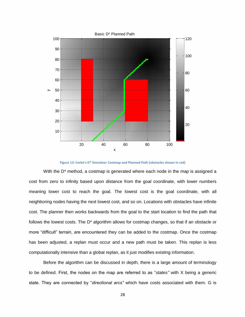
Roadmap method, and the toolbox’s code for these algorithms is used as a starting point. An
example of a D* planned path is shown below, where the start point is on the bottom edge of the
graph at coordinates (30, 1), and the goal is at (80, 80) (see Figure 13).
28
Figure 13: Corke’s D* Simulator Costmap and Planned Path (obstacles shown in red)
With the D* method, a costmap is generated where each node in the map is assigned a
cost from zero to infinity based upon distance from the goal coordinate, with lower numbers
meaning lower cost to reach the goal. The lowest cost is the goal coordinate, with all
neighboring nodes having the next lowest cost, and so on. Locations with obstacles have infinite
cost. The planner then works backwards from the goal to the start location to find the path that
follows the lowest costs. The D* algorithm allows for costmap changes, so that if an obstacle or
more “difficult” terrain, are encountered they can be added to the costmap. Once the costmap
has been adjusted, a replan must occur and a new path must be taken. This replan is less
computationally intensive than a global replan, as it just modifies existing information.
Before the algorithm can be discussed in depth, there is a large amount of terminology
to be defined. First, the nodes on the map are referred to as “states” with X being a generic
state. They are connected by “directional arcs” which have costs associated with them. G is
x
y
Basic D* Planned Path
20 40 60 80 100
10
20
30
40
50
60
70
80
90
100
20
40
60
80
100
120
29
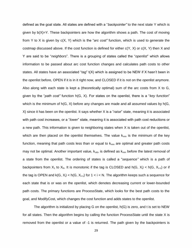
defined as the goal state. All states are defined with a “backpointer” to the next state Y which is
given by b(X)=Y. These backpointers are how the algorithm shows a path. The cost of moving
from Y to X is given by c(X, Y) which is the “arc cost” function, which is used to generate the
costmap discussed above. If the cost function is defined for either c(Y, X) or c(X, Y) then X and
Y are said to be “neighbors”. There is a grouping of states called the “openlist” which allows
information to be passed about arc cost function changes and calculates path costs to other
states. All states have an associated “tag” t(X) which is assigned to be NEW if X hasn’t been in
the openlist before, OPEN if it is in it right now, and CLOSED if it is not on the openlist anymore.
Also along with each state is kept a (theoretically optimal) sum of the arc costs from X to G,
given by the “path cost” function h(G, X). For states on the openlist, there is a “key function”
which is the minimum of h(G, X) before any changes are made and all assumed values by h(G,
X) since it has been on the openlist. It says whether X is a “raise” state, meaning it is associated
with path cost increases, or a “lower” state, meaning it is associated with path cost reductions or
a new path. This information is given to neighboring states when X is taken out of the openlist,
which are then placed on the openlist themselves. The value kmin is the minimum of the key
function, meaning that path costs less than or equal to kmin are optimal and greater path costs
may not be optimal. Another important value, kold, is defined as kmin before the latest removal of
a state from the openlist. The ordering of states is called a “sequence” which is a path of
backpointers from X1 to XN. It is monotonic if the tag is CLOSED and h(G, Xi) < h(G, Xi+1) or if
the tag is OPEN and k(G, Xi) < h(G, Xi+1) for 1 < i < N. The algorithm keeps such a sequence for
each state that is or was on the openlist, which denotes decreasing current or lower-bounded
path costs. The primary functions are ProcessState, which looks for the best path costs to the
goal, and ModifyCost, which changes the cost function and adds states to the openlist.
The algorithm is initialized by placing G on the openlist, h(G) is zero, and t is set to NEW
for all states. Then the algorithm begins by calling the function ProcessState until the state X is
removed from the openlist or a value of -1 is returned. The path given by the backpointers is

30
then followed until the robot either reaches the goal or detects an obstacle in its path. If the
latter occurs the ModifyCost function is used to change the cost function and adds the states
whose cost has changed to the openlist. Pseudocode for the algorithm is shown in Figure 14
[59].
31
Figure 14: D* Pseudocode
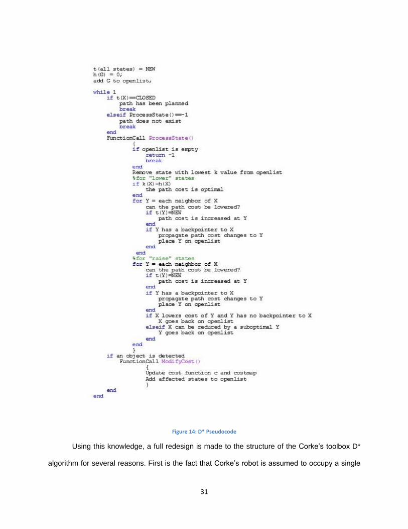
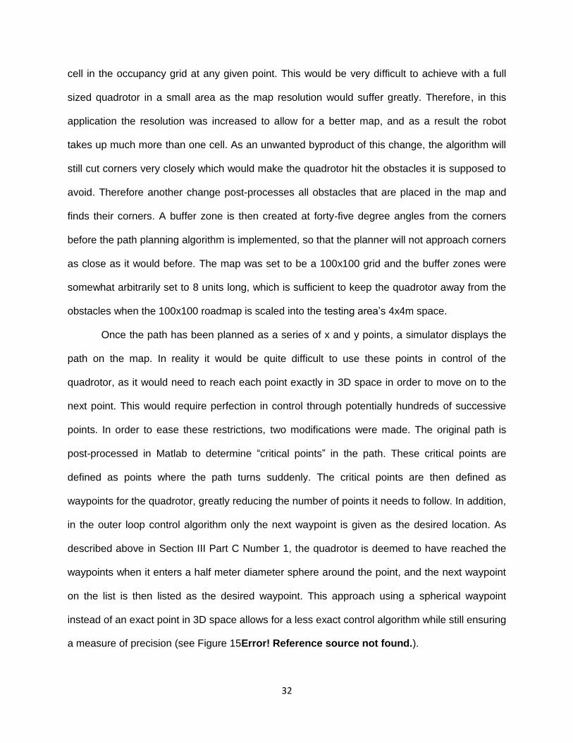
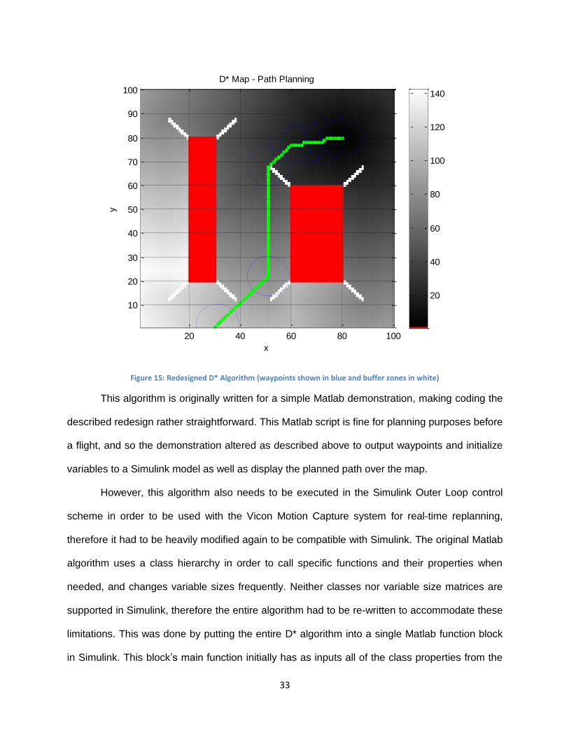
Using this knowledge, a full redesign is made to the structure of the Corke’s toolbox D*
algorithm for several reasons. First is the fact that Corke’s robot is assumed to occupy a single
32
cell in the occupancy grid at any given point. This would be very difficult to achieve with a full
sized quadrotor in a small area as the map resolution would suffer greatly. Therefore, in this
application the resolution was increased to allow for a better map, and as a result the robot
takes up much more than one cell. As an unwanted byproduct of this change, the algorithm will
still cut corners very closely which would make the quadrotor hit the obstacles it is supposed to
avoid. Therefore another change post-processes all obstacles that are placed in the map and
finds their corners. A buffer zone is then created at forty-five degree angles from the corners
before the path planning algorithm is implemented, so that the planner will not approach corners
as close as it would before. The map was set to be a 100x100 grid and the buffer zones were
somewhat arbitrarily set to 8 units long, which is sufficient to keep the quadrotor away from the
obstacles when the 100x100 roadmap is scaled into the testing area’s 4x4m space.
Once the path has been planned as a series of x and y points, a simulator displays the
path on the map. In reality it would be quite difficult to use these points in control of the
quadrotor, as it would need to reach each point exactly in 3D space in order to move on to the
next point. This would require perfection in control through potentially hundreds of successive
points. In order to ease these restrictions, two modifications were made. The original path is
post-processed in Matlab to determine “critical points” in the path. These critical points are
defined as points where the path turns suddenly. The critical points are then defined as
waypoints for the quadrotor, greatly reducing the number of points it needs to follow. In addition,
in the outer loop control algorithm only the next waypoint is given as the desired location. As
described above in Section III Part C Number 1, the quadrotor is deemed to have reached the
waypoints when it enters a half meter diameter sphere around the point, and the next waypoint
on the list is then listed as the desired waypoint. This approach using a spherical waypoint
instead of an exact point in 3D space allows for a less exact control algorithm while still ensuring
a measure of precision (see Figure 15Error! Reference source not found.).
33
Figure 15: Redesigned D* Algorithm (waypoints shown in blue and buffer zones in white)
This algorithm is originally written for a simple Matlab demonstration, making coding the
described redesign rather straightforward. This Matlab script is fine for planning purposes before
a flight, and so the demonstration altered as described above to output waypoints and initialize
variables to a Simulink model as well as display the planned path over the map.
However, this algorithm also needs to be executed in the Simulink Outer Loop control
scheme in order to be used with the Vicon Motion Capture system for real-time replanning,
therefore it had to be heavily modified again to be compatible with Simulink. The original Matlab
algorithm uses a class hierarchy in order to call specific functions and their properties when
needed, and changes variable sizes frequently. Neither classes nor variable size matrices are
supported in Simulink, therefore the entire algorithm had to be re-written to accommodate these
limitations. This was done by putting the entire D* algorithm into a single Matlab function block
in Simulink. This block’s main function initially has as inputs all of the class properties from the
x
y
D* Map - Path Planning
20 40 60 80 100
10
20
30
40
50
60
70
80
90
100
20
40
60
80
100
120
140
34
Matlab planner and calls all necessary sub-functions which are listed below the main function.
The properties are then each passed into and then out of all subsequent function calls so that
they may be used or modified as needed. The main function then outputs the final values of
these properties, which are fed back into the function block as inputs for the next time step. All
properties and other matrices are initialized to a fixed size and kept that size throughout the
entire function block to ensure compatibility.
2. Probabilistic Roadmap Method
The other map based planning algorithm is the Probabilistic Roadmap method, which
was tested to compare with D*. This method uses an occupancy grid roadmap with obstacles
defined as having a value of one and traversable areas having a value of zero. There are two
phases to this method, the learning phase and the query phase. In the learning phase, the
algorithm chooses a set number of randomly generated nodes, or configurations of the robot,
that do not lie in the obstacles. It then iterates through each node and assigns an edge between
it and all neighboring nodes that are closer than a certain threshold to denote that they are
connected, meaning the robot may travel along the edge. This is all completed without needing
the start and goal nodes. Once all nodes and edges are assigned, the query phase begins. The
start and goal points are defined, the algorithm connects them to the closest nodes. The planner
is asked to choose a path from the closest node to the start point to the closest node to the end
point. There is no built-in replanning function similar to D*. Instead, the occupancy grid must be
modified and a global replan must occur, choosing new points and edges around the obstacles.
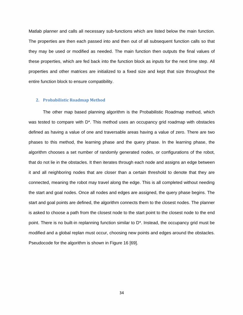
Pseudocode for the algorithm is shown in Figure 16 [69].
35
Figure 16: PRM Pseudocode
36
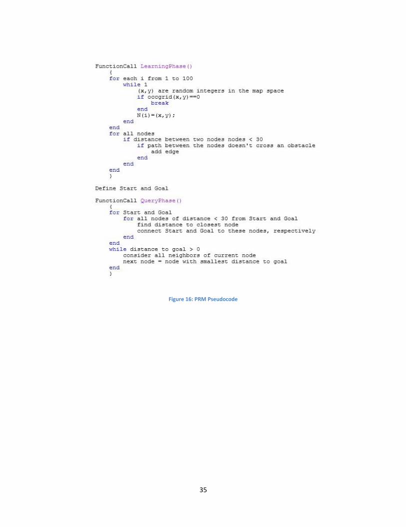
Figure 17: PRM Planned Path
For this specific application, once again the map is set to be a 100x100 grid. Node
selection was changed to take into account an area around all of the obstacles as a buffer zone.
The buffer zone is to ensure none of the points would be “too close” to the obstacles for the
quadrotor to traverse by them, and was chosen to be the eight nodes in all directions around the
obstacles. One hundred nodes were used, and edges were only assigned between nodes that
were closer than thirty units. Generally this achieves adequate results, however the path may
sometimes seem to be somewhat arbitrary or indirect due to the random nature of the node
selection. However, instead of needing a post-processed path to choose the waypoints, the
planner was simply modified to output the nodes that were chosen, shown in yellow in Figure 17
above. Note the start and end nodes are again (30, 1) and (80, 80), respectively.
x
y
Basic PRM Planned Path
10 20 30 40 50 60 70 80 90 100
10
20
30
40
50
60
70
80
90
100
37
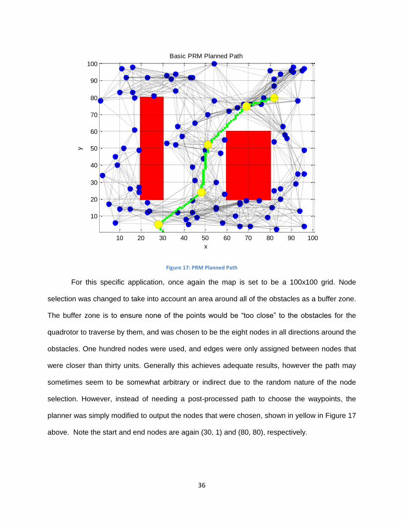
Figure 18: Modified PRM algorithm
A Matlab script planner was constructed to output the initial waypoints in the same way
as the D* function. Next, the PRM function was modified for use in Simulink in exactly the same
way as the D* function, with all properties from the Matlab planner’s classes were inputs to the
Simulink PRM replanner function. These properties are treated exactly the same as for the D*
planner by being passed through all function calls.
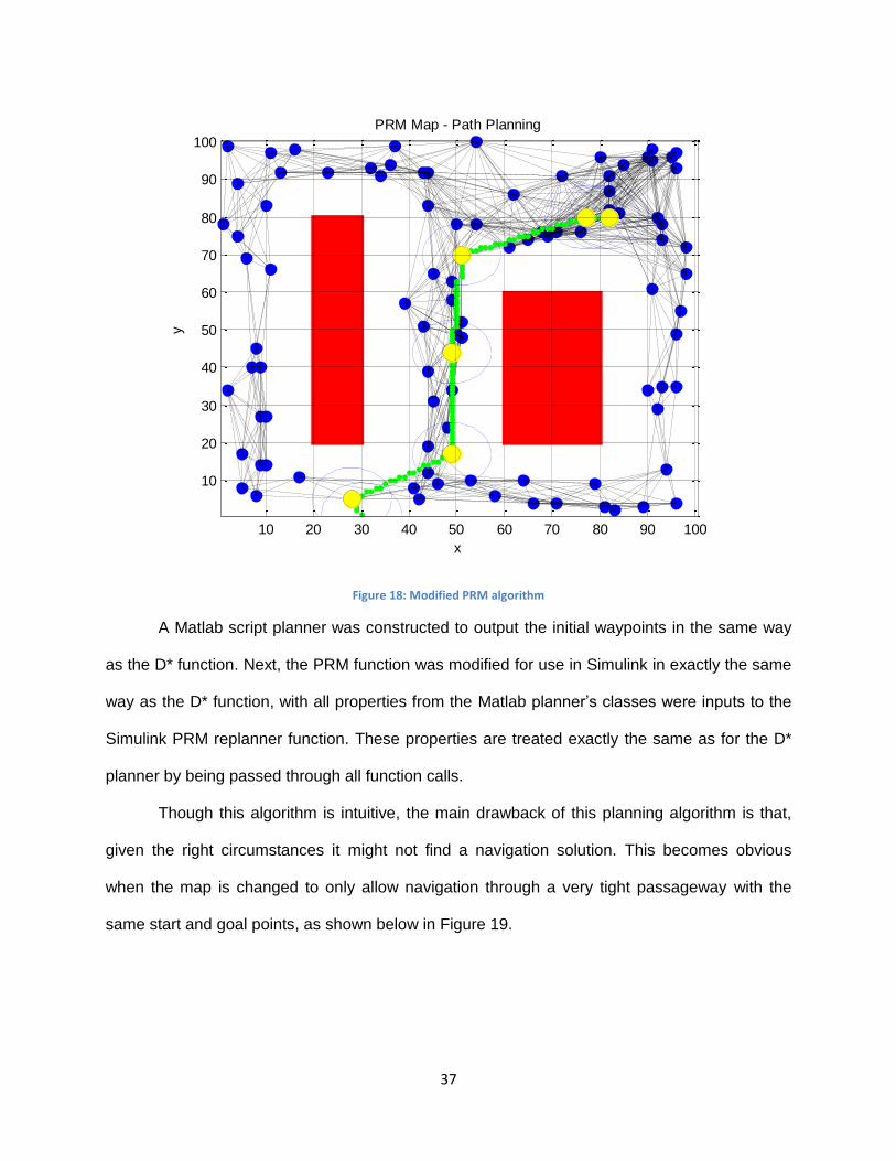
Though this algorithm is intuitive, the main drawback of this planning algorithm is that,
given the right circumstances it might not find a navigation solution. This becomes obvious
when the map is changed to only allow navigation through a very tight passageway with the
same start and goal points, as shown below in Figure 19.
x
y
PRM Map - Path Planning
10 20 30 40 50 60 70 80 90 100
10
20
30
40
50
60
70
80
90
100
38
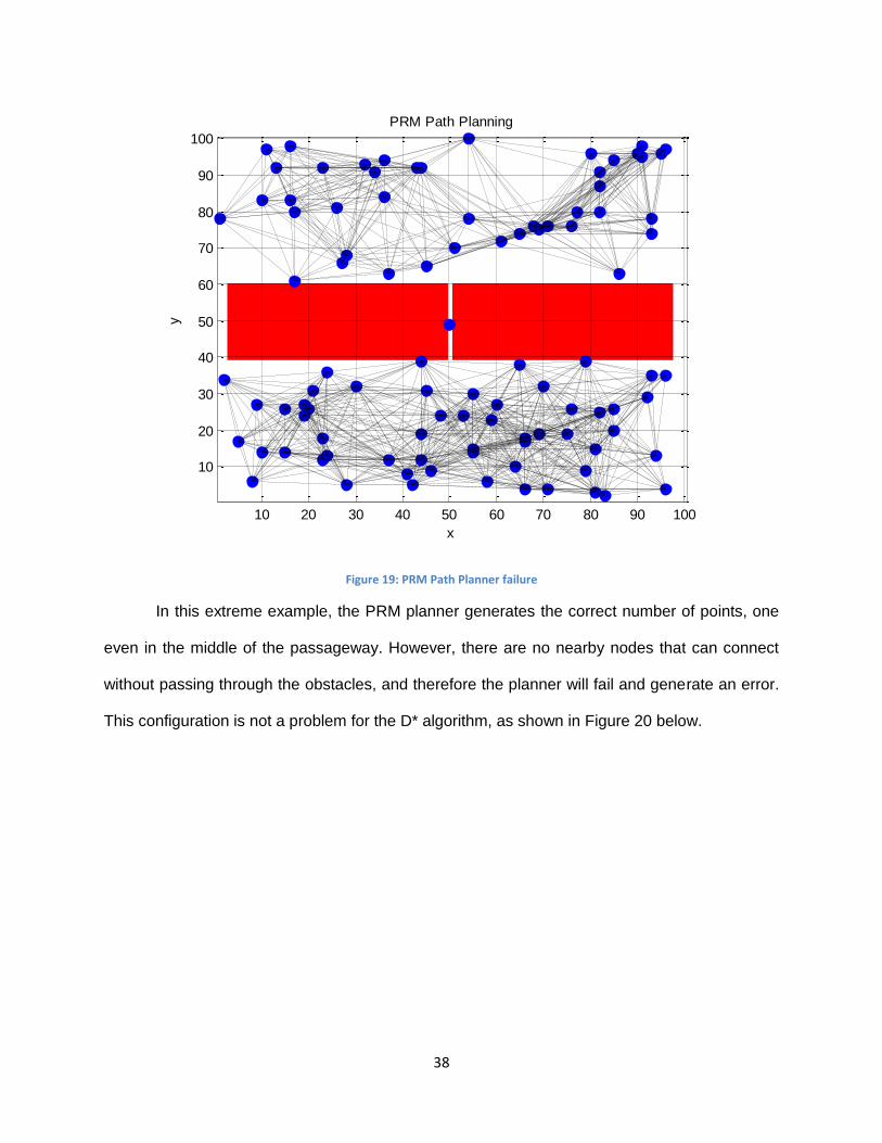
Figure 19: PRM Path Planner failure
In this extreme example, the PRM planner generates the correct number of points, one
even in the middle of the passageway. However, there are no nearby nodes that can connect
without passing through the obstacles, and therefore the planner will fail and generate an error.
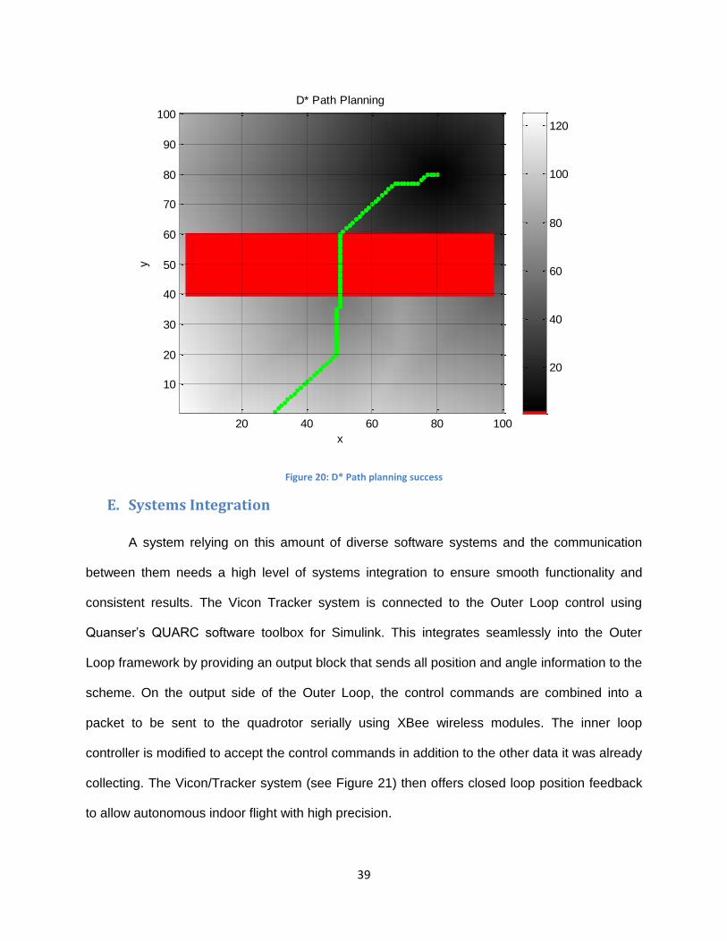
This configuration is not a problem for the D* algorithm, as shown in Figure 20 below.
x
y
PRM Path Planning
10 20 30 40 50 60 70 80 90 100
10
20
30
40
50
60
70
80
90
100
39
Figure 20: D* Path planning success
E. Systems Integration
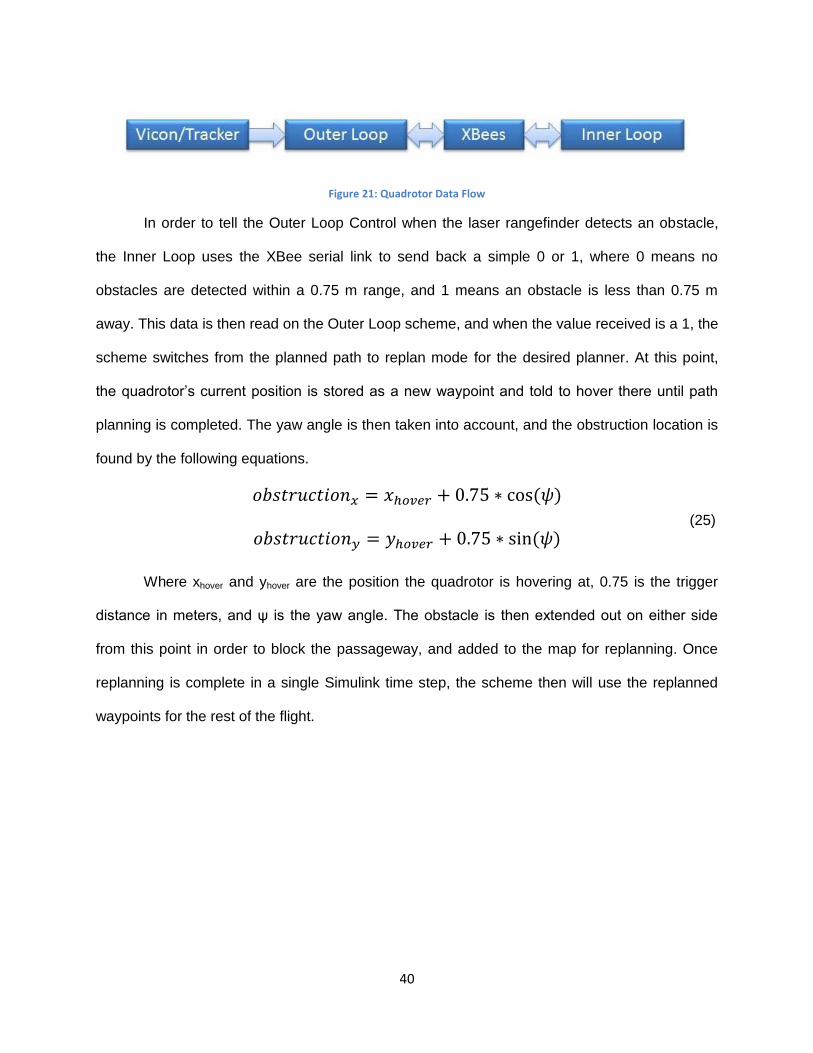
A system relying on this amount of diverse software systems and the communication
between them needs a high level of systems integration to ensure smooth functionality and
consistent results. The Vicon Tracker system is connected to the Outer Loop control using
Quanser’s QUARC software toolbox for Simulink. This integrates seamlessly into the Outer
Loop framework by providing an output block that sends all position and angle information to the
scheme. On the output side of the Outer Loop, the control commands are combined into a
packet to be sent to the quadrotor serially using XBee wireless modules. The inner loop
controller is modified to accept the control commands in addition to the other data it was already
collecting. The Vicon/Tracker system (see Figure 21) then offers closed loop position feedback
to allow autonomous indoor flight with high precision.
x
y
D* Path Planning
20 40 60 80 100
10
20
30
40
50
60
70
80
90
100
20
40
60
80
100
120
40
Figure 21: Quadrotor Data Flow
In order to tell the Outer Loop Control when the laser rangefinder detects an obstacle,
the Inner Loop uses the XBee serial link to send back a simple 0 or 1, where 0 means no
obstacles are detected within a 0.75 m range, and 1 means an obstacle is less than 0.75 m
away. This data is then read on the Outer Loop scheme, and when the value received is a 1, the
scheme switches from the planned path to replan mode for the desired planner. At this point,
the quadrotor’s current position is stored as a new waypoint and told to hover there until path
planning is completed. The yaw angle is then taken into account, and the obstruction location is
found by the following equations.
𝑜𝑏𝑠𝑡𝑟𝑢𝑐𝑡𝑖𝑜𝑛𝑥 = 𝑥ℎ𝑜𝑣𝑒𝑟 + 0.75 ∗ cos(𝜓)
𝑜𝑏𝑠𝑡𝑟𝑢𝑐𝑡𝑖𝑜𝑛𝑦 = 𝑦ℎ𝑜𝑣𝑒𝑟 + 0.75 ∗ sin(𝜓) (25)
Where xhover and yhover are the position the quadrotor is hovering at, 0.75 is the trigger
distance in meters, and ψ is the yaw angle. The obstacle is then extended out on either side
from this point in order to block the passageway, and added to the map for replanning. Once
replanning is complete in a single Simulink time step, the scheme then will use the replanned
waypoints for the rest of the flight.
41
IV. Testing
A. Simulation
Before flight testing, both path planning algorithms were tested in Matlab to see how
they would perform, to provide a stepping stone to real-life implementation, and to ensure
replanning was viable. The same map to be used for flight testing is used here as well as the
same start and goal nodes, (30, 1) and (80, 80).
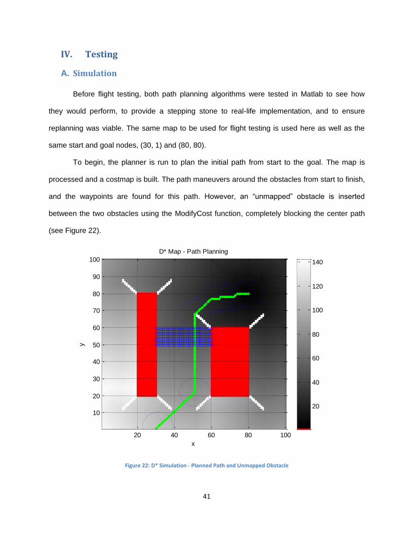
To begin, the planner is run to plan the initial path from start to the goal. The map is
processed and a costmap is built. The path maneuvers around the obstacles from start to finish,
and the waypoints are found for this path. However, an “unmapped” obstacle is inserted
between the two obstacles using the ModifyCost function, completely blocking the center path
(see Figure 22).
Figure 22: D* Simulation - Planned Path and Unmapped Obstacle
x
y
D* Map - Path Planning
20 40 60 80 100
10
20
30
40
50
60
70
80
90
100
20
40
60
80
100
120
140
42
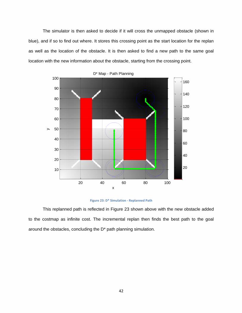
The simulator is then asked to decide if it will cross the unmapped obstacle (shown in
blue), and if so to find out where. It stores this crossing point as the start location for the replan
as well as the location of the obstacle. It is then asked to find a new path to the same goal
location with the new information about the obstacle, starting from the crossing point.
Figure 23: D* Simulation - Replanned Path
This replanned path is reflected in Figure 23 shown above with the new obstacle added
to the costmap as infinite cost. The incremental replan then finds the best path to the goal
around the obstacles, concluding the D* path planning simulation.
x
y
D* Map - Path Planning
20 40 60 80 100
10
20
30
40
50
60
70
80
90
100
20
40
60
80
100
120
140
160
43
Figure 24: PRM Simulation - Planned Path with Unmapped Obstacle
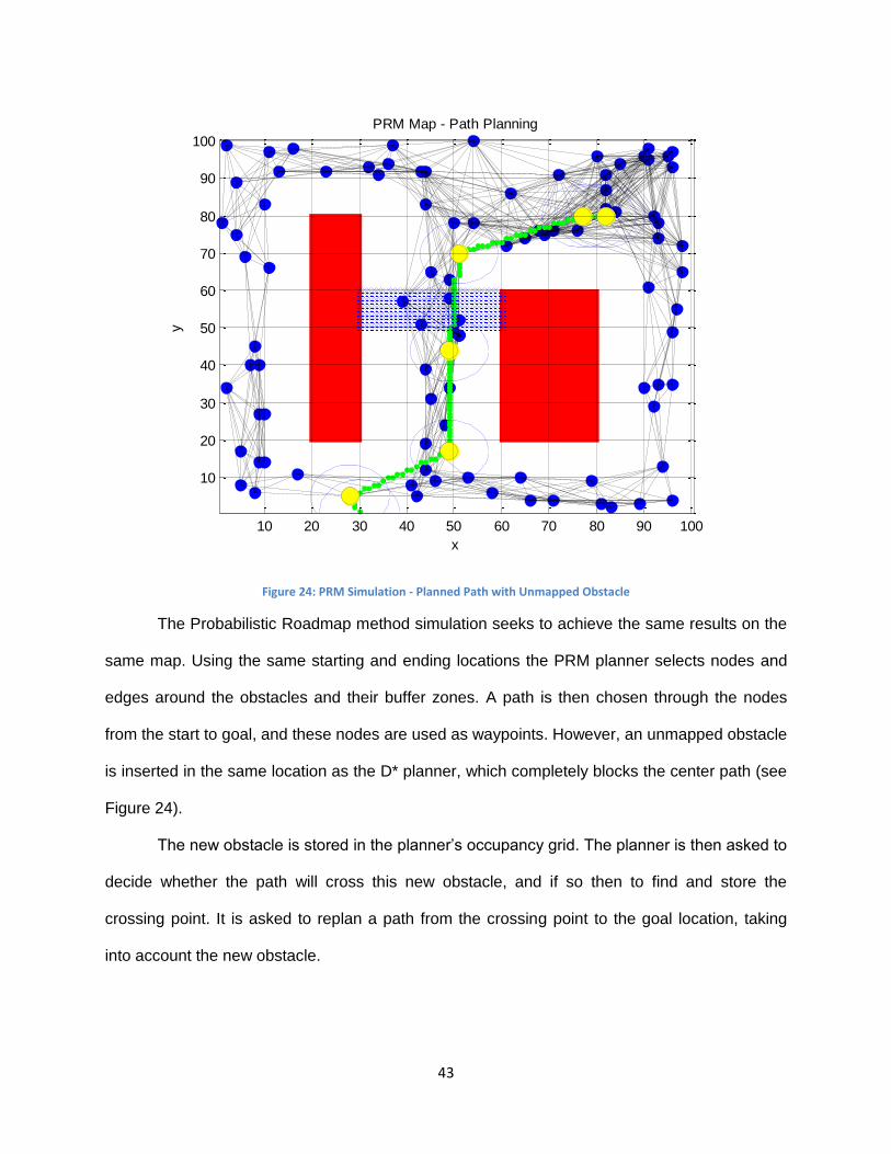
The Probabilistic Roadmap method simulation seeks to achieve the same results on the
same map. Using the same starting and ending locations the PRM planner selects nodes and
edges around the obstacles and their buffer zones. A path is then chosen through the nodes
from the start to goal, and these nodes are used as waypoints. However, an unmapped obstacle
is inserted in the same location as the D* planner, which completely blocks the center path (see
Figure 24).
The new obstacle is stored in the planner’s occupancy grid. The planner is then asked to
decide whether the path will cross this new obstacle, and if so then to find and store the
crossing point. It is asked to replan a path from the crossing point to the goal location, taking
into account the new obstacle.
x
y
PRM Map - Path Planning
10 20 30 40 50 60 70 80 90 100
10
20
30
40
50
60
70
80
90
100
44
Figure 25: PRM Simulation - Replanned Path
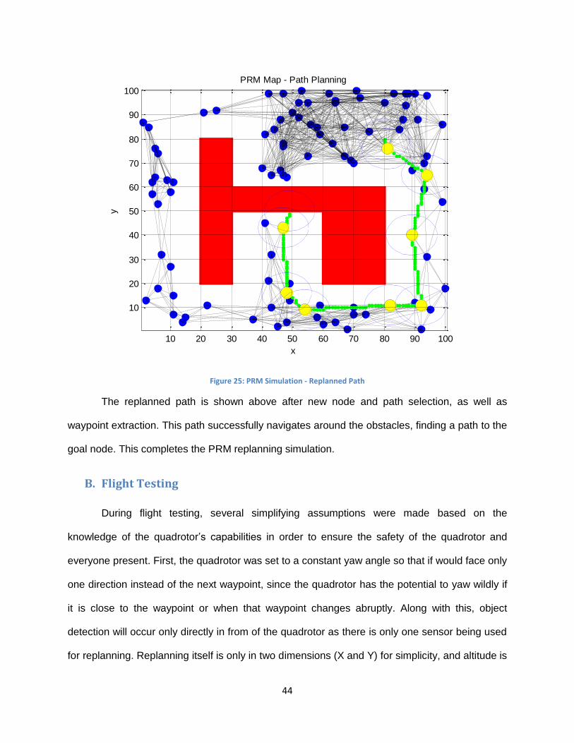
The replanned path is shown above after new node and path selection, as well as
waypoint extraction. This path successfully navigates around the obstacles, finding a path to the
goal node. This completes the PRM replanning simulation.
B. Flight Testing
During flight testing, several simplifying assumptions were made based on the
knowledge of the quadrotor’s capabilities in order to ensure the safety of the quadrotor and
everyone present. First, the quadrotor was set to a constant yaw angle so that if would face only
one direction instead of the next waypoint, since the quadrotor has the potential to yaw wildly if
it is close to the waypoint or when that waypoint changes abruptly. Along with this, object
detection will occur only directly in from of the quadrotor as there is only one sensor being used
for replanning. Replanning itself is only in two dimensions (X and Y) for simplicity, and altitude is
x
y
PRM Map - Path Planning
10 20 30 40 50 60 70 80 90 100
10
20
30
40
50
60
70
80
90
100
45
held constant during flight. In addition, there are no actual physical obstacles in the testing area
during flight in order to reduce risk of crash or injury to bystanders. Also, replanning will only
occur once per flight, and the detected object will be assumed to block the entirety of the path
between the two mapped obstacles.
During test flights, a safety pilot controls an RC transmitter communicating with an RC
receiver on the quadrotor’s autopilot board. The pilot may manually supersede autonomous
flight if needed to ensure that the quadrotor will not do anything undesirable or unsafe. Another
person monitors the Outer Loop Simulink control scheme on the ground station computer, and
may alternate the quadrotor’s flight mode between hover and execution of waypoint following. A
third person wearing a helmet and safety goggles maneuvers an obstacle during flight for the
quadrotor to detect.
Before D* flight, the Matlab D* path planner is run to initialize all parameters for the
Simulink Outer Loop scheme. It uses the same map as well as start and goal nodes as the
simulation, plans waypoints from the start to the goal, and then adds preprogrammed
intermediate waypoints around the outside of the leftmost obstacle to allow the quadrotor to
return to start, and in this way continually repeat the planned waypoints (see Figure 26). Note
that the figure below is shown in the room’s 4x4 meter space with the origin in the center and
not the planner’s 100x100 space with the origin in the bottom left corner. Also note the axes are
different from normal convention, as the vertical axis is the Inertial Frame’s X-axis, and the
horizontal axis is the Inertial Frame’s Y-axis, and that the values shown on the Y-axis are
negative. While somewhat confusing, this is to allow consistent views of the objects and
waypoints. Therefore, using the point (50, 50) as the origin of this space, the starting point of the
algorithm is converted from (30, 1) in the planner’s coordinates to (-1.5, 0.5) in the Inertial
Frame’s coordinates.
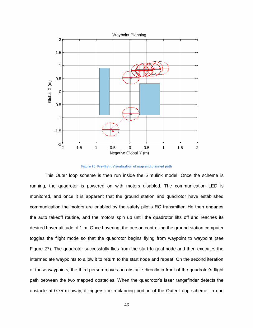
46
Figure 26: Pre-flight Visualization of map and planned path
This Outer loop scheme is then run inside the Simulink model. Once the scheme is
running, the quadrotor is powered on with motors disabled. The communication LED is
monitored, and once it is apparent that the ground station and quadrotor have established
communication the motors are enabled by the safety pilot’s RC transmitter. He then engages
the auto takeoff routine, and the motors spin up until the quadrotor lifts off and reaches its
desired hover altitude of 1 m. Once hovering, the person controlling the ground station computer
toggles the flight mode so that the quadrotor begins flying from waypoint to waypoint (see
Figure 27). The quadrotor successfully flies from the start to goal node and then executes the
intermediate waypoints to allow it to return to the start node and repeat. On the second iteration
of these waypoints, the third person moves an obstacle directly in front of the quadrotor’s flight
path between the two mapped obstacles. When the quadrotor’s laser rangefinder detects the
obstacle at 0.75 m away, it triggers the replanning portion of the Outer Loop scheme. In one
-2 -1.5 -1 -0.5 0 0.5 1 1.5 2-2
-1.5
-1
-0.5
0
0.5
1
1.5
2
Negative Global Y (m)
Waypoint Planning
Glo
bal X
(m
)
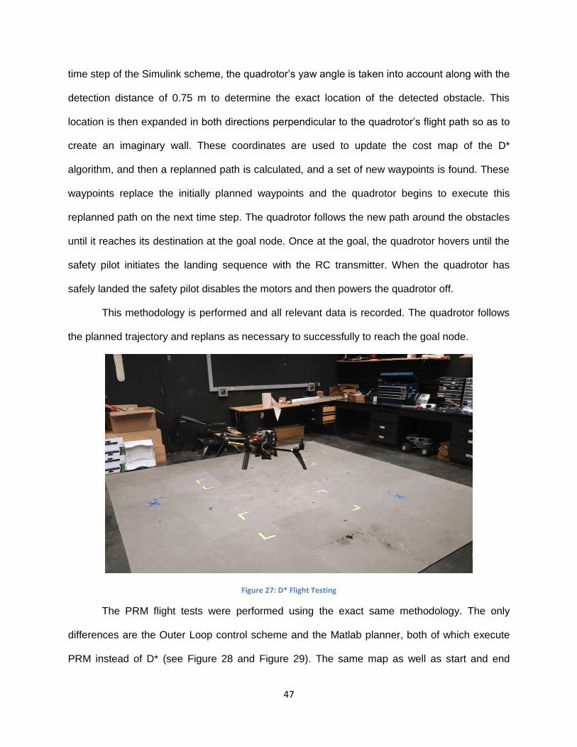
47
time step of the Simulink scheme, the quadrotor’s yaw angle is taken into account along with the
detection distance of 0.75 m to determine the exact location of the detected obstacle. This
location is then expanded in both directions perpendicular to the quadrotor’s flight path so as to
create an imaginary wall. These coordinates are used to update the cost map of the D*
algorithm, and then a replanned path is calculated, and a set of new waypoints is found. These
waypoints replace the initially planned waypoints and the quadrotor begins to execute this
replanned path on the next time step. The quadrotor follows the new path around the obstacles
until it reaches its destination at the goal node. Once at the goal, the quadrotor hovers until the
safety pilot initiates the landing sequence with the RC transmitter. When the quadrotor has
safely landed the safety pilot disables the motors and then powers the quadrotor off.
This methodology is performed and all relevant data is recorded. The quadrotor follows
the planned trajectory and replans as necessary to successfully to reach the goal node.
Figure 27: D* Flight Testing
The PRM flight tests were performed using the exact same methodology. The only
differences are the Outer Loop control scheme and the Matlab planner, both of which execute
PRM instead of D* (see Figure 28 and Figure 29). The same map as well as start and end
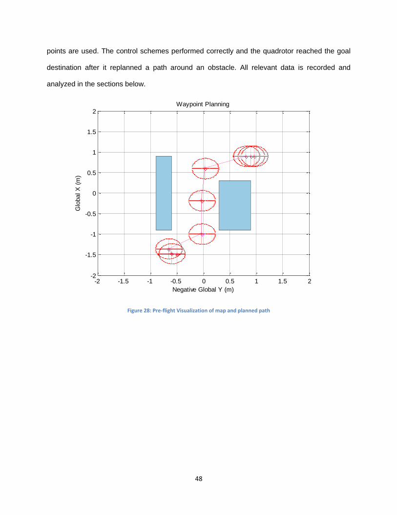
48
points are used. The control schemes performed correctly and the quadrotor reached the goal
destination after it replanned a path around an obstacle. All relevant data is recorded and
analyzed in the sections below.
Figure 28: Pre-flight Visualization of map and planned path
-2 -1.5 -1 -0.5 0 0.5 1 1.5 2-2
-1.5
-1
-0.5
0
0.5
1
1.5
2
Negative Global Y (m)
Waypoint Planning
Glo
bal X
(m
)
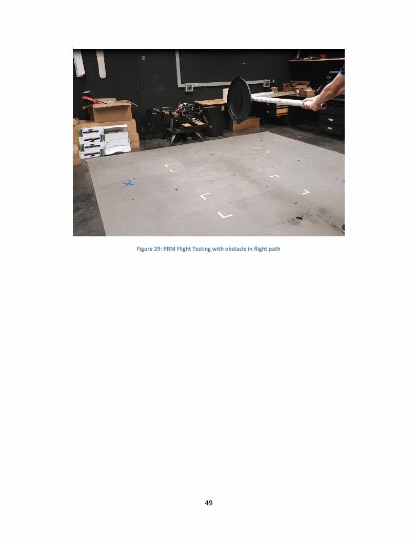
49
Figure 29: PRM Flight Testing with obstacle in flight path
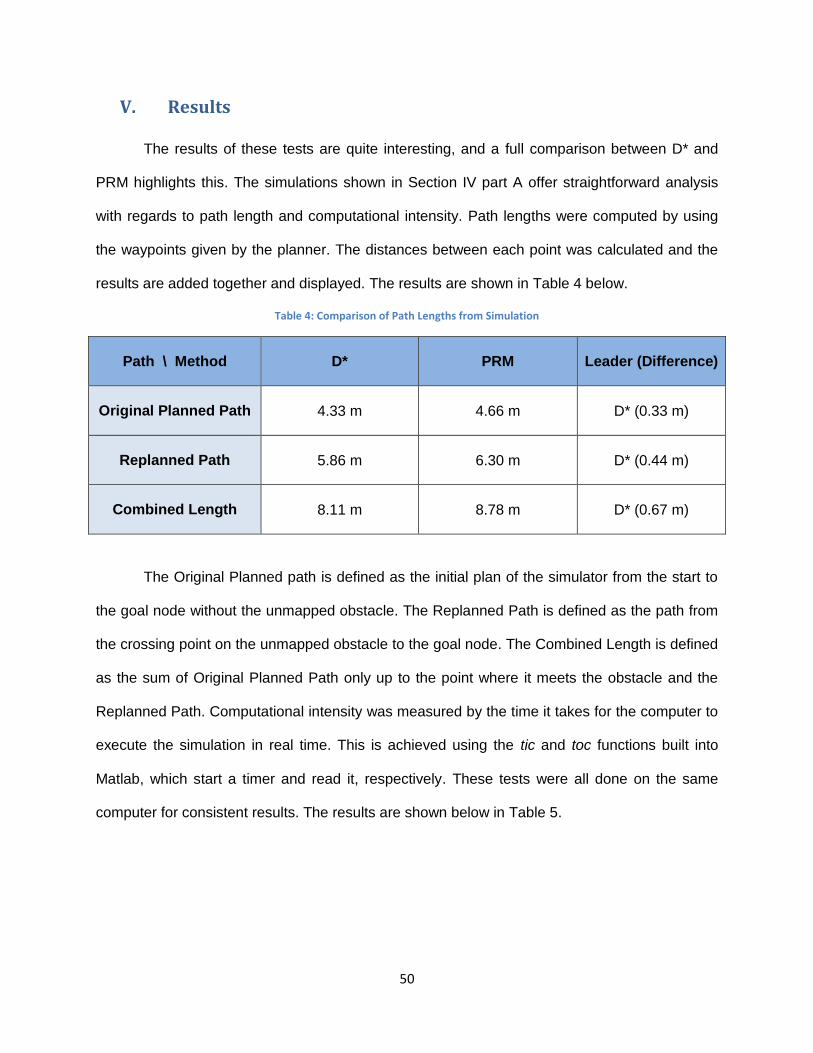
50
V. Results
The results of these tests are quite interesting, and a full comparison between D* and
PRM highlights this. The simulations shown in Section IV part A offer straightforward analysis
with regards to path length and computational intensity. Path lengths were computed by using
the waypoints given by the planner. The distances between each point was calculated and the
results are added together and displayed. The results are shown in Table 4 below.
Table 4: Comparison of Path Lengths from Simulation
Path \ Method D* PRM Leader (Difference)
Original Planned Path 4.33 m 4.66 m D* (0.33 m)
Replanned Path 5.86 m 6.30 m D* (0.44 m)
Combined Length 8.11 m 8.78 m D* (0.67 m)
The Original Planned path is defined as the initial plan of the simulator from the start to
the goal node without the unmapped obstacle. The Replanned Path is defined as the path from
the crossing point on the unmapped obstacle to the goal node. The Combined Length is defined
as the sum of Original Planned Path only up to the point where it meets the obstacle and the
Replanned Path. Computational intensity was measured by the time it takes for the computer to
execute the simulation in real time. This is achieved using the tic and toc functions built into
Matlab, which start a timer and read it, respectively. These tests were all done on the same
computer for consistent results. The results are shown below in Table 5.
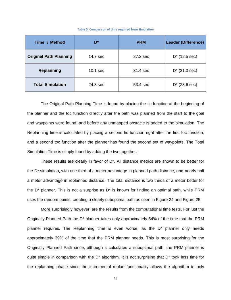
51
Table 5: Comparison of time required from Simulation
Time \ Method D* PRM Leader (Difference)
Original Path Planning 14.7 sec 27.2 sec D* (12.5 sec)
Replanning 10.1 sec 31.4 sec D* (21.3 sec)
Total Simulation 24.8 sec 53.4 sec D* (28.6 sec)
The Original Path Planning Time is found by placing the tic function at the beginning of
the planner and the toc function directly after the path was planned from the start to the goal
and waypoints were found, and before any unmapped obstacle is added to the simulation. The
Replanning time is calculated by placing a second tic function right after the first toc function,
and a second toc function after the planner has found the second set of waypoints. The Total
Simulation Time is simply found by adding the two together.
These results are clearly in favor of D*. All distance metrics are shown to be better for
the D* simulation, with one third of a meter advantage in planned path distance, and nearly half
a meter advantage in replanned distance. The total distance is two thirds of a meter better for
the D* planner. This is not a surprise as D* is known for finding an optimal path, while PRM
uses the random points, creating a clearly suboptimal path as seen in Figure 24 and Figure 25.
More surprisingly however, are the results from the computational time tests. For just the
Originally Planned Path the D* planner takes only approximately 54% of the time that the PRM
planner requires. The Replanning time is even worse, as the D* planner only needs
approximately 39% of the time that the PRM planner needs. This is most surprising for the
Originally Planned Path since, although it calculates a suboptimal path, the PRM planner is
quite simple in comparison with the D* algorithm. It is not surprising that D* took less time for
the replanning phase since the incremental replan functionality allows the algorithm to only
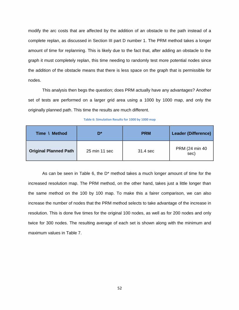
52
modify the arc costs that are affected by the addition of an obstacle to the path instead of a
complete replan, as discussed in Section III part D number 1. The PRM method takes a longer
amount of time for replanning. This is likely due to the fact that, after adding an obstacle to the
graph it must completely replan, this time needing to randomly test more potential nodes since
the addition of the obstacle means that there is less space on the graph that is permissible for
nodes.
This analysis then begs the question; does PRM actually have any advantages? Another
set of tests are performed on a larger grid area using a 1000 by 1000 map, and only the
originally planned path. This time the results are much different.
Table 6: Simulation Results for 1000 by 1000 map
Time \ Method D* PRM Leader (Difference)
Original Planned Path 25 min 11 sec 31.4 sec PRM (24 min 40
sec)
As can be seen in Table 6, the D* method takes a much longer amount of time for the
increased resolution map. The PRM method, on the other hand, takes just a little longer than
the same method on the 100 by 100 map. To make this a fairer comparison, we can also
increase the number of nodes that the PRM method selects to take advantage of the increase in
resolution. This is done five times for the original 100 nodes, as well as for 200 nodes and only
twice for 300 nodes. The resulting average of each set is shown along with the minimum and
maximum values in Table 7.
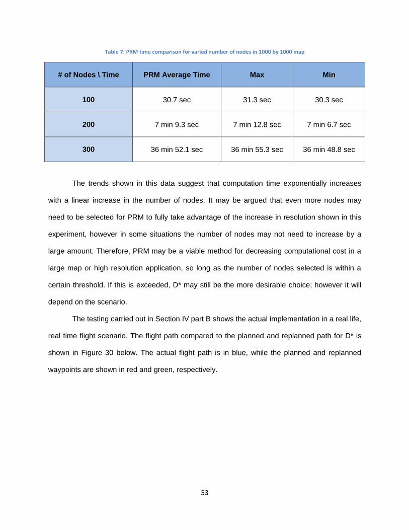
53
Table 7: PRM time comparison for varied number of nodes in 1000 by 1000 map
# of Nodes \ Time PRM Average Time Max Min
100 30.7 sec 31.3 sec 30.3 sec
200 7 min 9.3 sec 7 min 12.8 sec 7 min 6.7 sec
300 36 min 52.1 sec 36 min 55.3 sec 36 min 48.8 sec
The trends shown in this data suggest that computation time exponentially increases
with a linear increase in the number of nodes. It may be argued that even more nodes may
need to be selected for PRM to fully take advantage of the increase in resolution shown in this
experiment, however in some situations the number of nodes may not need to increase by a
large amount. Therefore, PRM may be a viable method for decreasing computational cost in a
large map or high resolution application, so long as the number of nodes selected is within a
certain threshold. If this is exceeded, D* may still be the more desirable choice; however it will
depend on the scenario.
The testing carried out in Section IV part B shows the actual implementation in a real life,
real time flight scenario. The flight path compared to the planned and replanned path for D* is
shown in Figure 30 below. The actual flight path is in blue, while the planned and replanned
waypoints are shown in red and green, respectively.
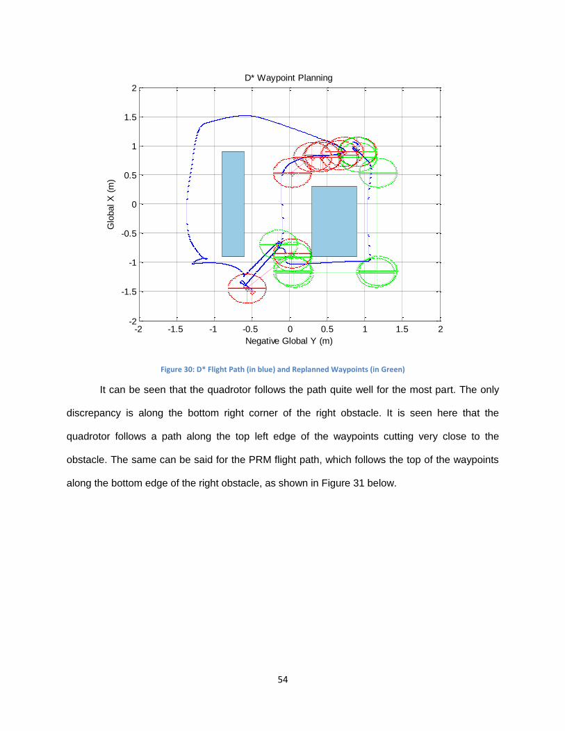
54
Figure 30: D* Flight Path (in blue) and Replanned Waypoints (in Green)
It can be seen that the quadrotor follows the path quite well for the most part. The only
discrepancy is along the bottom right corner of the right obstacle. It is seen here that the
quadrotor follows a path along the top left edge of the waypoints cutting very close to the
obstacle. The same can be said for the PRM flight path, which follows the top of the waypoints
along the bottom edge of the right obstacle, as shown in Figure 31 below.
-2 -1.5 -1 -0.5 0 0.5 1 1.5 2-2
-1.5
-1
-0.5
0
0.5
1
1.5
2
Negative Global Y (m)
D* Waypoint Planning
Glo
bal X
(m
)
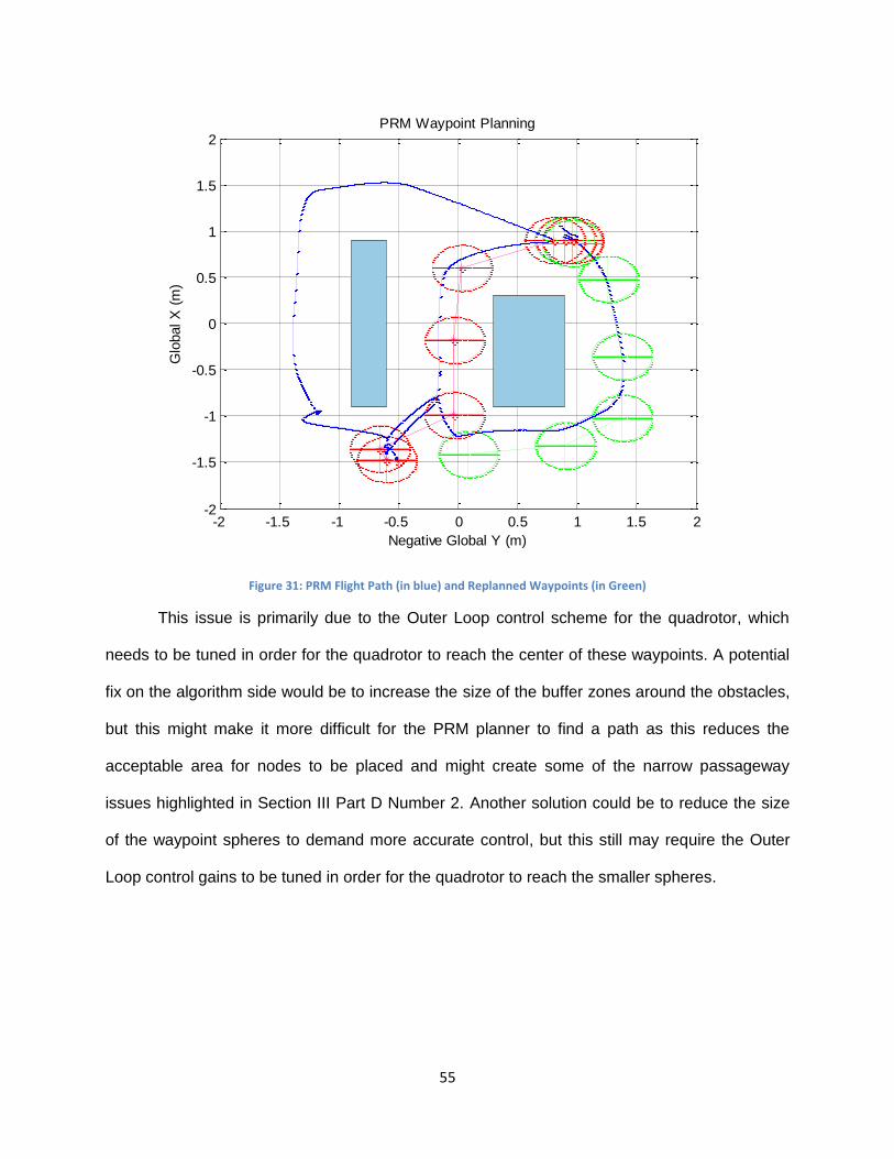
55
Figure 31: PRM Flight Path (in blue) and Replanned Waypoints (in Green)
This issue is primarily due to the Outer Loop control scheme for the quadrotor, which
needs to be tuned in order for the quadrotor to reach the center of these waypoints. A potential
fix on the algorithm side would be to increase the size of the buffer zones around the obstacles,
but this might make it more difficult for the PRM planner to find a path as this reduces the
acceptable area for nodes to be placed and might create some of the narrow passageway
issues highlighted in Section III Part D Number 2. Another solution could be to reduce the size
of the waypoint spheres to demand more accurate control, but this still may require the Outer
Loop control gains to be tuned in order for the quadrotor to reach the smaller spheres.
-2 -1.5 -1 -0.5 0 0.5 1 1.5 2-2
-1.5
-1
-0.5
0
0.5
1
1.5
2
Negative Global Y (m)
PRM Waypoint Planning
Glo
bal X
(m
)
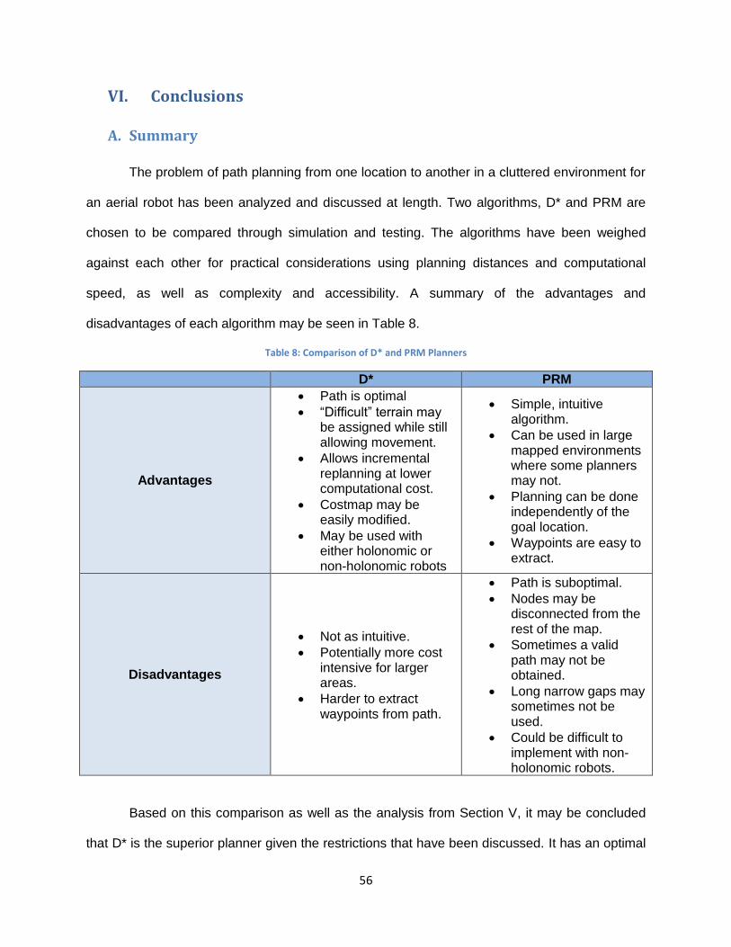
56
VI. Conclusions
A. Summary
The problem of path planning from one location to another in a cluttered environment for
an aerial robot has been analyzed and discussed at length. Two algorithms, D* and PRM are
chosen to be compared through simulation and testing. The algorithms have been weighed
against each other for practical considerations using planning distances and computational
speed, as well as complexity and accessibility. A summary of the advantages and
disadvantages of each algorithm may be seen in Table 8.
Table 8: Comparison of D* and PRM Planners
D* PRM
Advantages
Path is optimal
“Difficult” terrain may be assigned while still allowing movement.
Allows incremental replanning at lower computational cost.
Costmap may be easily modified.
May be used with either holonomic or non-holonomic robots
Simple, intuitive algorithm.
Can be used in large mapped environments where some planners may not.
Planning can be done independently of the goal location.
Waypoints are easy to extract.
Disadvantages
Not as intuitive.
Potentially more cost intensive for larger areas.
Harder to extract waypoints from path.
Path is suboptimal.
Nodes may be disconnected from the rest of the map.
Sometimes a valid path may not be obtained.
Long narrow gaps may sometimes not be used.
Could be difficult to implement with non-holonomic robots.
Based on this comparison as well as the analysis from Section V, it may be concluded
that D* is the superior planner given the restrictions that have been discussed. It has an optimal
57
path to the goal which may be achieve by holonomic and non-holonomic robots alike, and
requires much less computational intensity. It can plan a path through nearly any environment,
making it situationally independent. Its only drawbacks might be increased computational cost
when scaling to a larger map, waypoints are harder to find, and the algorithm itself is not as
straightforward. Although the PRM method easily gives waypoints and is readily understood, it
generates a suboptimal path that may not be suitable for non-holonomic robots. It also may not
generate a path through narrow passageways unless an additional method is applied. Testing
shows that this method also takes more computational power for this application, though if
expanded to a larger map PRM might very well be the better choice.
B. Future Work
In order to achieve outdoor flight, the quadrotor will need an accurate position estimation
system to replace the Vicon system. The best answer is to use Global Positioning System
(GPS). To get GPS readings, a Novatel OEM-V1 GPS receiver may be interfaced with the
quadrotor’s avionics board. This has been tested to ensure GPS lock is reliable and consistent.
While GPS is a reliable method for outdoor position estimation, its accuracy is generally quite
low for an application such as this. Inertial navigation data to determine position could be used
and would be highly accurate initially, but the integration process incurs compounding errors
which cause drift almost immediately. To remedy this problem, an Extended Kalman Filter
(EKF) may be used. An EKF is a recursive nonlinear estimator that can combine measurements
using prediction and update phases. In order to restrict the somewhat inaccurate GPS
measurements, IMU gyroscope data and accelerometer integration is incorporated for its
smoothness and consistency. On the other hand, GPS keeps the accelerometer integration
within a certain region over time so that they do not drift too much. This actually allows the best
parts of both measurements to be put together to achieve position estimation convergence. An
58
Extended Kalman Filter, which has been tested previously on fixed wing autonomous flight, will
be used for outdoor position estimation.
For outdoor flights a terrain following method will need to be implemented instead of
constant altitude control. This will allow the quadrotor to stay at a consistent altitude going up or
down hills or flying over any low obstacles. This has been tested using an ultrasonic rangefinder
instead of the laser rangefinder used for object detection, mainly due to the fact that the
ultrasonic rangefinder has a detection cone in front of it, where the laser rangefinder only has a
narrow beam for detection. Testing has proven this method to be effective indoors, however
more testing is necessary before reliable outdoor implementation.
In addition, the PC104 computer will need to be re-implemented into the system to
handle Outer Loop control duties for outdoor flights. This will allow flight without a ground
station, as discussed earlier, making the quadrotor a much more flexible platform without relying
on wireless communication for outdoor control.
Finally, the map used for the planning algorithms will have to be expanded for outdoor
applications to allow for larger scale flights. These flights will cover much more area, so a larger
map will be necessary while retaining a similar resolution for accurate obstacle avoidance. This
will likely increase the processing time needed for the D* algorithm, while the PRM method
should not be greatly affected. This has the potential to swing the preferred algorithm in the
favor of the PRM method if D* is drastically more computationally intensive. Further experiments
and testing will need to verify this.
59
References
[1] Leishman, "The Bréguet-Richet Quad-Rotor Helicopter of 1907," University of Maryland, 2015.
[2] Hirschberg, "The American Helicopter: An Overview of Helicopter Developments in America. 1908-
1999," American Helicopter Society, 2000.
[3] Wannberg, "The Quadrotor Platform from a military point of view," Etteplan, 2012.
[4] Quora, "Why aren't quadrotors used in helicopters rather than the design we see today," Quora,
2014. [Online]. Available: http://www.quora.com/Why-arent-quadrotors-used-in-helicopters-
rather-than-the-design-we-see-today. [Accessed 20 June 2015].
[5] "Black Knight Transformer," Advanced Tactics, Inc., 2015. [Online]. Available:
https://www.advancedtacticsinc.com/technology/black-knight/. [Accessed 15 June 2015].
[6] "E-volo," E-volo, 2015. [Online]. Available: http://www.e-volo.com/. [Accessed 15 June 2015].
[7] C. Wood, "A closer look at the Malloy Aeronautics Hoverbike," Gizmag, 19 August 2014. [Online].
Available: http://www.gizmag.com/closer-look-malloy-aeronautics-hoverbike/33414/. [Accessed 15
June 2015].
[8] K. Atherton, "The US Army Wants its own Hoverbike, Again," Popular Science, 22 June 2015.
[Online]. Available: http://www.popsci.com/pentagon-funding-actual-hoverbike?image=0.
[Accessed 25 June 2015].
[9] A. M. Stoll, J. Bevirt, P. P. Pei and E. V. Stilson, "Conceptual Design of the Joby S2 Electric VTOL
PAV," in Aviation Technology, Integration, and Operations Conference, Atlanta, Georgia, 2015.
[10] N. E. Serrano, Autonomous Quadrotor Unamnned Aerial Vehicle for Culvert Inspection,
Massachusetts Institute of Technology, 2011.
[11] T. K. Venugopalan, T. Taher and G. Barbastathis, "Autonomous Landing of an Unmanned Aerial
Vehicle on an Autonomous Marine Vehicle," IEEE, Singapore, 2012.
[12] R. Sampaio, A. Herneandes, M. Becker, F. Catalano, F. Zanini, J. Nobrega and C. Martins, "SquidCop:
Design and Evaluation of a Novel Quadrotor MAV for In-flight Launching Air-to-Ground Missions,"
IEEE, pp. 1-10, 2014.
[13] J. Borenstein, "The HoverBot - An Electrically Powered Flying Robot," Department of Mechanical
Engineering and Applied Mechanics, The University of Michigan, Ann Arbor, MI, 1993.
60
[14] R. Briand, B. Bluteau and O. Patrouix, "Desing and control of an Outdoor Autonomous Quadrotor
powered by a four strokes RC engine," IEEE, Bidart, France, 2006.
[15] E. Cetinsoy, S. Dikyar, C. Hancer, K. T. Oner, E. Sirimoglu, M. Unel and M. Aksit, "Design and
construction of a novel quad tilt-wing UAV," Mechatronics, vol. 22, no. 6, p. 723–745, 2012.
[16] R. Huang, Y. Liu and J. J. Zhu, "Guidance, Navigation, and Control System Design for Tripropeller
Vertical-Takeoff-and-Landing Unmanned Air Vehicle," Journal of Aircraft, vol. 46, no. 6, pp. 1837-
1856, 2009.
[17] M. Miwa, S. Uemura, Y. Ishihara, A. Imamura, J.-h. Shim and K. Ioi, "Evaluation of quad ducted-fan
helicopter," International Journal of Intelligent Unmanned Systems, vol. 1, no. 2, pp. 187-198, 2013.
[18] K. LaFleur, K. Cassady, A. Doud, K. Shades, E. Rogin and B. He, "Quadcopter control in three-
dimensional spance using a noninvasinve motor imagery-based brain-computer interface," Journal
of Neural Engineering, vol. 10, no. 4, 2013.
[19] C. Doyle, J. Bird, T. Isom, J. Kallman, D. Bareiss, D. Dunlop, R. King, J. Abbott and M. Minor, "An
Avian-Inspired Passive Mechanism for Quadrotor Perching," IEEE/ASME Transactions on
Mechatronics, vol. 18, no. 2, pp. 506-517, 2013.
[20] K. Mohta, V. Kumar and K. Daniilidis, "Vision-based Control of a Quadrotor for Perching on LInes," in
IEEE International Conference on Robotics and Automation, Hong Kong, 2014.
[21] J. Yeol and C.-H. Lin, "Development of Multi-Tentacle Micro Air Vehicle," in International Conference
on Unmanned Aircraft Systems, Orlando, FL, 2014.
[22] M. J. Cutler, "Design and Control of an Autonomous Variable-Pitch Quadrotor Helicopter,"
Massachusetts Institute of Technology, Cambridge, Massachusetts, 2012.
[23] M. Cutler, N. K. Ure, B. Michini and J. How, "Comparison of Fixed and Variable Pitch Actuators for
Agile Quadrotors," in AIAA Guidance, Navigation, and Control Conference, Minneapolis, MInnesota,
2012.
[24] M. Muller, S. Lupashin and R. D'Andrea, "Quadrocopter Ball Juggling," in IEEE/RSJ International
Conference on Intelligent Robots and Systems, San Francisco, CA, USA, 2011.
[25] M. Hehn and R. D'Andrea, "A Flying Inverted Pendulum," in IEEE International Conference on
Robotics and Automation, Shanghai, China, 2011.
[26] S. Lupashin, A. Schollig, M. Sherback and R. D'Andrea, "A Simple Learning Strategy for High-Speed
Quadrocopter Multi-Flips," in IEEE International Conference on Robotics and Automation,
Anchorage, Alaska, USA, 2010.
61
[27] E. Davis, B. Nizette and C. Yu, "Development of a Low Cost Quadrotor Platform for Swarm
Experiments," in 32nd Chinese Control Conference, Xi'an, 2013.
[28] J. Leonard, A. Savvaris and A. Tsourdos, "Towards a Fully Autonomous Swarm of Unmanned Aerial
Vehicles," in UKACC International Conference on Control, Cardiff, UK, 2012.
[29] A. Kushleyev, D. Mellinger and V. Kumar, "Towards A Swarm of Agile Micro Quadrotors,"
Autonomous Robots, vol. 35, no. 4, pp. 287-300, 2013.
[30] L. Chaimowicz, N. Michael and V. Kumar, "Controlling Swarms of Robots Using Interpolated Implicit
Functions," in International Conference on Robotics and Automation, Barcelona, Spain, 2005.
[31] J. How, E. King and Y. Kuwata, "Flight Demonstrations of Cooperative Control for UAV Teams," in
AIAA 3rd "Unmanned Unlimited" Technical Conference, Workshop and Exhibit, Chicago, Illinois,
2004.
[32] M. A. Guney and M. Unel, "Formation Control of a Group of Micro Aerial Vehicles (MAVs)," in IEEE
International Conference on Systems, Man, and Cybernetics, Manchester, 2013.
[33] Q. Lindsey, D. Mellinger and V. Kumar, "Construction of Cubic Structures with Quadrotor Teams,"
MIT Press, Cambridge, Massachusetts, 2012.
[34] S. R. B. dos Santos, S. N. Givigi Jr and C. L. N. Junior, "Autonomous Construction of Structures in a
Dynamic Environment using Reinforcement Learning," in IEEE International Systems Conference,
Orlando, FL, 2013.
[35] M. S. Alvissalim, B. Zaman, A. H. Z., M. A. Ma'sum, G. Jati, W. Jatmiko and P. Mursanto, "Swarm
Quadrotor Robots for Telecommunication Network Coverage Area Expansion in Disaster Area," in
SICE Annual Conference, Akita, Japan, 2012.
[36] R. Ritz and R. D'Andrea, "Carrying a Flexible Payload with Multiple Flying Vehicles," in IEEE/RSJ
International Conference on Intelligent Robots and Systems (IROS), Tokyo, Japan, 2013.
[37] R. Ritz, M. W. Muller, M. Hehn and R. D'Andrea, "Cooperative Quadrocopter Ball Throwing and
Catching," in IEEE/RSJ Interational Conference on Intelligent Robots and Systems, Vilamoura,
Algarve, Portugal, 2012.
[38] F. Augugliaro, A. P. Schoellig and R. D'Andrea, "Dance of the Flying Machines: Methods for
Designing and Executing an Aerial Dance Choreography," IEEE Robotics & Automation Magazine,
vol. 20, no. 4, pp. 96-104, 2013.
[39] M. Waibel, "Controlling a Quadrotor Using Kinect," IEEE Spectrum, 2 July 2011. [Online]. Available:
http://spectrum.ieee.org/automaton/robotics/robotics-software/quadrotor-interaction. [Accessed
62
21 June 2015].
[40] R. Oung, F. Bourgault, M. Donovan and R. D'Andrea, "The Distributed Flight Array," in IEEE
International Conference on Robotics and Automation, Anchorage, Alaska, USA, 2010.
[41] E. W. Dijkstra, "A Note on Two Problems in Connexion with Graphs," Numerische Mathematik, pp.
269-271, 1959.
[42] H. Juzoji, I. Nakajima and T. Kitano, "A Development of Network Topology of Wireless Packet
Communications for Disaster Situation with Genetic Algorithms or with Dijkstra's," in IEEE
International Conference on Communications, Kyoto, 2011.
[43] M. Parulekar, V. Padte, T. Shah, K. Shroff and R. Shetty, "Automatic Vehicle Navigation using
Dijkstra's Algorithm," in ICATE, Mumbai, 2013.
[44] Y. Yi and Y. Guan, "A Path Planning Method to Robot Soccer Based on Dijkstra Algorithm," in
Advances in ECWAC, 2012.
[45] P. W. Eklund, S. Kirkby and S. Pollitt, "A Dynamic Multi-source Dijkstra's Algorithm for Vehicle
Routing," in Australian New Zealand Conference on Intelligent Information Systems, Adelaide,
Australia, 1996.
[46] Z. Yan and Z. Jun, "Dijkstra's Algorithm Based Robus Optimization to Airline Network Planning," in
International Conference on Mechanic Automation and Control Engineering, Wuhan, 2010.
[47] L. Verscheure, L. Peyrodie, N. Makni, N. Betrouni, S. Maouche and M. Vermandel, "Dijkstra's
Algorithm Applied to 3D Skeletonization of the Brain Vascular Tree: Evaluation and Application to
Symbolic," in IEEE EMBS, Buenos Aires, Argentine, 2010.
[48] N. Anastopoulos, K. Nikas, G. Goumas and N. Koziris, "Early Experiences on Accelerating Dijkstra's
Algorithm Using Transactional Memory," in IEEE International Symposium on Parallel & Distributed
Processing, Rome, 2009.
[49] N. Jasika, N. Alispahic, A. Elma, K. Ilvana, L. Elma and N. Nosovic, "Dijkstra's shortest path algorithm
serial and parallel execution performance analysis," in MIPRO, Opatija, Croatia, 2012.
[50] J.-R. Jiang, H.-W. Huang, J.-H. Liao and S.-Y. Chen, "Extending Dijkstra's Shortest Path Algorithm for
Software Defined Networking," in Asia-Pacific Network Operations and Management Symposium,
Hsinchu, 2014.
[51] D. Fan and P. Shi, "Improvements of Dijkstra's Algorithm and Its Application in Route Planning," in
International Conference on Fuzzy Systems and Knowledge Discovery, Yantai, Shandong, 2010.
63
[52] A. Felner, "Position Paper: Dijkstra's Algorithm versus Uniform Cost Search or a Case Against
Dijkstra's Algorithm," in Association for the Advancement of Artificial Intelligence, 2011.
[53] P. E. Hart, N. J. Nilsson and B. Raphael, "A Formal Basis for the Heuristic Determination of Minimum
Cost Paths," IEEE Transactions of Systems Science and Cybernetics, vol. 4, no. 2, pp. 100-107, 1968.
[54] W. Zeng and R. L. Church, "Finding shortest paths on real road networks: the case for A*,"
International Journal of Geographical Information Science, vol. 23, no. 4, pp. 531-543, 2009.
[55] J. Yao, C. Lin, X. Xie, A. J. Wang and C.-C. Hung, "Path Planning for Virtual Human Motion Using
Improved A* Algorithm," in International Conference on Information Technology, Las Vegas, NV,
2010.
[56] H.-K. Lee, W. Jeong, S. Lee and J. Won, "A Hierarchical Path Planning of cleaning robot Based on
Grid Map," in International Conference on Consumer Electronics, Las Vegas, NV, 2013.
[57] M. Ghallab and D. Allard, "Ae — An Efficient Near Admissible Heristic Search Algorithm," in IJCAI,
Karlsruhe, Germany, 1983.
[58] H. Wang, J. Zhou, G. Zheng and Y. Liang, "HAS: Hierarchical A-Star algorithm for big map navigation
in special areas," in International Conference on Digital Home, Guangzhou, 2014.
[59] A. Stentz, "Optimal and Efficient Path Planning for Partially-Known Environments," in International
Conference on Robotics and Automation, 1994.
[60] A. Stentz, "The Focussed D* Algorithm for Real-Time Replanning," in International Joint Conference
on Artificial Intelligence, 1995.
[61] S. Koenig and M. Likhachev, "Improved Fast Replanning for Robot Navigation in Unknown Terrain,"
in International Conference on Robotics & Automation, Washington, DC, 2002.
[62] D. Ferguson and A. Stentz, "The Delayed D* Algorithm for Efficient Path Replanning," in
International Conference on Robotics and Automation, Barcelona, Spain, 2005.
[63] M. Likhachev, D. Ferguson, G. Gordon, A. Stentz and S. Thrun, "Anytime Dynamic A*: An Anytime,
Replanning Algorithm," in International Conference on Automated Planning and Scheduling, 2005.
[64] V. Ganapathy, S. C. Yun and T. W. Chien, "Enhanced D* Lite Algorithm for Autonomous Mobile
Robot," International Journal of Applied Science and Technology, vol. 1, no. 1, pp. 58-73, 2011.
[65] X. Che, D. Liu and T. Tang, "Path Planning for UCAV in Dynamic and Uncertain Environments Based
on Focused D* Algorithm," in International Symposium on Computational Intelligence and Design,
Hangzhou, 2011.
64
[66] M. Seder, K. Macek and I. Petrovic, "An integrated approach to real-time mobile robot control in
partially known indoor environments," in Annual Conference of IEEE Industrial Electronics Society,
2005.
[67] M. Seder and I. Petrovic, "Integration of Focused D* and Witkowski's algorithm for path planning
and replanning," in European Conference on Mobile Robots, 2009.
[68] S. Karaman and E. Frazzoli, "Sampling-based Algorithms for Optimal Motion Planning," International
Journal of Robotics Research, vol. 30, no. 7, pp. 846-894, 2011.
[69] L. E. Kavraki, P. Svestka, J.-C. Latombe and M. H. Overmars, "Probabilistic Roadmaps for Path
Planning in High-Dimensional Configuration Spaces," IEEE Transactions of Robotics and Automation,
vol. 12, no. 4, pp. 566-580, 1996.
[70] N. Malone, K. Manavi, J. Wood and L. Tapia, "Construction and Use of Roadmaps That Incorporate
Workspace Modeling Errors," in IEEE/RSJ International Conference on Intelligent Robots and
Systems, Tokyo, Japan, 2013.
[71] M. Sifyan, H. R. Topcuoglu and M. Ermis, "Path Planning for Mobile Sensor Platforms on a 3-D
Terrain Using Hybrid Evolutionary Algorithms," in IEEE Congress on Evolutionary Computation,
Barcelona, 2010.
[72] D. Aarno, D. Kragic and H. I. Christensen, "Artificial Potential Biased Probabilistic Roadmap
Method," in IEEE International Conference on Robotics and Automation, New Orleans, LA, 2004.
[73] B. Park and W. K. Chung, "Adaptive Node Sampling Method for Probabilistic Roadmap Planners," in
International Conference on Intelligent Robots and Systems, St. Louis, USA, 2009.
[74] Z. Jiandong and S. Jianbo, "Narrow Passages Identification for Probabilistic Roadmap Method," in
30th Chinese Control Conference, Yantai, China, 2011.
[75] A. Benitez, D. Vallejo and E. Medrano, "New Technique to Build Probabilistic Roadmap Methods," in
14th International Conference on Electronics, Communications and Computers, 2004.
[76] C. Ekenna, S. A. Jacobs, S. Thomas and N. M. Amato, "Adaptive Neighbor Connection for PRMs: A
Natural Fit for Heterogeneous Environments and Parallelism," in IEEE/RSJ International Conference
on Intelligent Robots and Systems, Tokyo, Japan, 2013.
[77] Q. Li, C. Wei, J. Wu and X. Zhu, "Improved PRM Method of Low Altitude Penetration Trajectory
Planning for UAVs," in IEEE Chinese Guidance, Navigation and Control Conference, Yantai, China,
2014.
[78] G. Wagner, M. Kang and H. Choset, "Probabilistic Path Planning for Multiple Robots with
65
Subdimensional Expansion," in IEEE International Conference on Robotics and Automation, Saint
Paul, Minnesota, 2012.
[79] J. Yang, P. Dymond and M. Jenkin, "Practicality-Based Probabilistic Roadmaps Method," in Canadian
Conference on Computer and Robot Vision, 2011.
[80] N. M. Amato and L. K. Dale, "Probabilistic Roadmap Methods are Embarrassingly Parallel," in
International Conference on Robotics and Automation, Detroit, Michigan, 1999.
[81] A. Tayebi and S. McGilvray, "Attitude stabilization of a four-rotor aerial robot," in IEEE Conference
on Decision and Control, Atlantis, Paradise Island, Bahamas, 2004.
[82] P. Corke, Robotics, Vision and Control, Berlin Heidelberg: Springer-Verlag, 2011.