pattern recognition based on statistics and … · not easy to extract relevant patterns from a...

The 10th International Conference “RELIABILITY and STATISTICS in TRANSPORTATION and COMMUNICATION - 2010”

1

Proceedings of the 10th International Conference “Reliability and Statistics in Transportation and Communication” (RelStat’10), 20–23 October 2010, Riga, Latvia, p. 1-10. ISBN 978-9984-818-34-4 Transport and Telecommunication Institute, Lomonosova 1, LV-1019, Riga, Latvia

PATTERN RECOGNITION BASED ON STATISTICS AND STRUCTURAL EQUATION MODELS IN MULTI-DIMENSIONAL

DATA WAREHOUSES OF SOCIAL BEHAVIORAL DATA

Dale Dzemydiene, Raimundas Vaitkevicius, Ignas Dzemyda

Mykolas Romeris University Ateities 20, Vilnius, LT-08303, Lithuania

E-mail: [email protected], [email protected], [email protected]

Multi-dimensional data in data warehouses (DWHs) can reveal problems related to data organization as well as informing

data mining techniques that can allow precise decisions to be made. It is not easy to extract relevant patterns from a large DWH. Using a suitable approach and a large number of pre-computations, the relational and multidimensional spaces of DWHs can be used to represent the aggregation space of OLAP (On-Line Analytical Processing) models. Our recent research has shown the benefits of using conceptual modeling of data warehouses integrated with data mining techniques based on linear equation methods. Data mining methods range from the simple discovery of frequent patterns and regularities to knowledge-based and interactive decision support processes in subject-oriented and integrated data warehouses (DWHs). Distinct tasks require different data structures and various data mining exercises. The approach of using statistical analysis and structural equation modeling methods in support of multiple analyses and semi-automatic pattern recognition processes is proposed. The multidimensional decision support system is integrated with the data mining technologies of social data warehouses. Ensembles of diverse and accurate classifiers are constructed on the bases of multidimensional classification methods and allow more sophisticated relations between variables of data analysis and factor analysis to be revealed. The paper describes an approach in which linear equation models are integrated with multiple statistical analysis and knowledge representation to recognize information patterns in data warehouses. The introduced methods of analysis allow us to practice control and to forecast the main social tendencies, as well as supporting decisions in different prevention tasks. The results of the application of the methods of statistical analysis are demonstrated by the social behavioral analysis data (for example, criminal analysis) of the some EU Countries.

Keywords: structural equation model, statistics, statistical databases, decision support system, data warehouse, multidimensional pattern recognition, factor analysis

1. Introduction Multi-dimensional data in data warehouses (DWHs) can reveal problems related to data

organization as well as informing data mining techniques that can allow precise decisions to be made. It is not easy to extract relevant patterns from a large DWH. Using a suitable approach and a large number of pre-computations, the relational and multidimensional spaces of DWHs can be used to represent the aggregation space of OLAP (On-Line Analytical Processing) models. Our recent research has shown the benefits of using conceptual modeling of data warehouses integrated with data mining techniques based on linear equation methods.

Data mining has several objectives. These include data analysis, assessment of risk and influencing factors and assessing profitability. General trends in society depend on social, political, and economic factors. Data mining can be one of the most significant indicators of these trends, reflecting the social and moral state of society [16, 17]. Some questions such as ‘what influences some social tendencies?’ become problematic to answer directly from the data space. Consequently, integrated methods of data mining and data structuring are required. Distinct tasks require different data structures and separate data mining exercises [10, 13, 14]. A series of organized actions in support of a cause can be analyzed separately because each case will involve patterns with a distinct signature. Mixing the analyses into one data mining exercise would simply dilute the differences between these signatures.

The knowledge that enables us to understand how to apply the methods of decision preparation is of special importance. Recent research has demonstrated the advantages of using ensembles of classifiers in classification problems. Ensembles of diverse and accurate base classifiers are constructed by machine-learning methods.

The development of ontological systems in this particular field requires the application of additional intelligent methods. These are intended to describe intricate decision situations and informal ways of arriving at a decision, etc. The decision support system under construction ensures ease of use and clarity of interpretation in the presentation of the results of analyses of data from the data warehouse of crime and social investigation.

Plenary Session

2

This paper describes an approach of using methods of data mining and factor analysis and making them automatically choose between different models in the decision support system. A structured analysis session commonly has three forms: discovery, prediction, and forensic analysis. Specific tasks are performed in each of these activities [11, 18]. The knowledge representation based on the ontological view of unified modeling language (UML) [4] is useful for the recognition of social behavioral information in such an analysis session. The time series analysis methods are introduced in a semi-structured analysis session of data mining. They allow us to exercise statistical control, forecast the main crime tendencies and support decisions relating to means of crime prevention. The results of the application are demonstrated by an analysis of EU Accession Countries crime record data from the important period of the ten years from 1990. 2. Knowledge Representation and Multi-dimensional Statistics for Analysis Session

The extraction of knowledge, trends, and patterns from within the data is an essential condition for

a qualified social behavioral situation evaluation. Such data may be evaluated by statistical or other econometric methods. The reliability evaluation of such statistics and the possibilities of choosing between methods in the manner of a semi–automatic component introduction for decision support systems is the main purpose of this research.

Conclusions and evaluated patterns of data analysis can influence future regarding the control and regulation of such processes in society, for example, crime detection, social control, and the development of prevention strategies. Recognition of unsustainable processes of social behavior at national and international levels is a complex phenomenon influenced by social, political and economical circumstances. For example, a crime rate is defined as the number of crimes per unit of population. A crime is considered registered if it is included in the centralized register of the state. The regional offices of crime statistics and research collect great volumes of data from different sources that reflect criminal events and their relations [20, 23]. These data are stored in warehouses with multiple variables and temporal dimensions.

Summarization may be used to reduce data size. However, summarization can also cause problems. Summarization of the same data set by two sampling or summarization methods may produce the same result, and summarization of the same data set by two methods may produce two different results [18]. An alternative approach could be to use a pattern recognition process in a data warehouse [10, 13, 19]. In this context, research patterns are characterized as generic structures derived from experience of modeling in past. These can be abstract, describing the structure of a model, or concrete, describing one particular model.

The knowledge representation process may be performed by special methods of artificial intelligence [1, 3, 9]. The knowledge that helps us to understand how to apply decision methods and develop advising systems is of special importance. Intellectual information systems have additional properties that enable structural analysis and data storage in the system, thereby modeling situations and making and explaining decisions [1, 3, 7]. In addition, the knowledge system must be able to abstract information and data about the current situation and to allow retrospective analysis and prognosis.

Multidimensional statistics, image identification, artificial intelligence, decision support and other methods compose the bases for data mining. Frequently these methods are interrelated. Five standard types of consistent patterns can be distinguished by fundamental data mining methods:

• an association characterizes the interdependence of some proceedings or events; • variation in time i.e. trends and interdependences in time series; • classification i.e. the evaluation of attributes which are typical of distinct groups of objects; • clusterization i.e. the segregation of homogeneous groups of data; • forecast i.e. finding system patterns that evaluate the adequacy and dynamics of process

variation with regard to the possibility of projecting these patterns into the future. To create models of the described types of patterns, the following main multidimensional

statistical methods are usually employed: • Cluster analysis. This multivariable method belongs to classification algorithms and solves the

problem of how to organize the observed data into meaningful structures which are not necessarily known in advance. The general categories of cluster analysis methods are: joining or tree clustering, two-way joint or block clustering and k-means clustering.

• Multiple regression. The general purpose of this well known family of methods is to analyze the relationship between several independent variables and a dependent variable. The regression function can be estimated, using the least squares estimation or any other loss function (nonlinear estimation). After the regression equation has been estimated, the prediction can be performed for a set of independent variables.


3

• Anova/Manova. The main purpose of the analysis of variance is to test for significant differences between the means of variables of interest. The variance between the means (treatment variance) is compared with error variance to test the hypothesis on a significant difference between the means. Anova is used for one dependent variable and Manova for two or more dependent (usually related) variables that are analyzed together [22, pp. 243-310].

• Discriminant function analysis [22, pp. 375-436]. In cases where the goal of the study is to identify the variables that discriminate between known groups, discriminant analysis is used. The basic idea underlying discriminant function analysis is to determine whether the groups differ with regard to the means of the variables. An additional question is to find out which variables can be best used to predict group membership.

• Logistic regression analysis. This is a form of multiple regression analysis where the independent (predicted) variable is of nominal measurement level (e.g. codes denoting groups or classes of interest in the data), and independent variables (predictors) are either nominal or continuous, measured on ratio/interval level. The method can be used for similar purposes to discriminant analysis. However, logistic regression analysis substantially relaxes some important assumptions of discriminant analysis, such as the normal distribution of values of the variables and homoscedasticity [22, p.441].

• Factor analysis. Factor analysis is used to reduce the number of variables and to detect structures in the relationships between the variables. Generally, as a method of simple data reduction, principal component analysis is often preferred, and principal factor analysis is more frequently used in cases when the goal of analysis is to detect some hypothetical structures (factors, or latent unobserved variables).

• Time series analysis. Time series analysis is based on the assumption that successive data values represent consecutive measurements taken at equally-spaced time intervals. Identifying the pattern of a phenomenon represented by the sequence of observations and predicting future events are the main goals of this analysis. In time series analysis, it is assumed usually that data consist of systemic patterns and random noise which, as a rule, obscures the patterns and makes them more difficult to identify.

• Log-linear analysis [22, pp. 858-912]. This type of analysis allows the testing of the various factors (nominal variables) that are used in cross tabulation, and their interactions, for statistical significance. The analysis of multi-way frequency tables, with two or more factors, is based on marginal frequencies (totals) of two or more factors. A minimal model, adequately describing frequencies in a multi-way table is often used.

• Hierarchical modeling or multi-level (linear) modeling [22, pp. 814-857]. Such models are used for research designs where the data is organized at more than one level. For example, students’ academic achievement is measured for pupils within classrooms, which are, in turn, nested within schools (schools can also be nested within regions or cities, regions within states, etc.).

• Structural Equation Modeling (also defined as covariance structure analysis, covariance structural modeling, analysis of covariance structures, causal modeling) [15, 21]. This is a family of related procedures which explicitly aim at the testing of complex data models (related to theories and hypotheses in the domain of interest), usually based on quantitative variables and their covariance matrixes.

The main types of such models are: path analysis models [15, pp. 93-122], confirmatory factor analysis models [15, pp. 165-208], structural regression models [15, pp. 209-236] and latent growth (change) models [6, 15, pp. 263-288]. Structural equation modeling is applied usually as a confirmatory data analysis technique, however, it can also be used for exploratory purposes [2]. Due to the relative novelty of SEM and its increasing popularity, in areas including criminology [12], a short introduction to SEM is presented. 3. Structural Equation Modeling

Structural Equation Modeling started approximately 90 years ago with the work of biometrician and geneticist Sewall Wright [24]. Wright introduced path analysis, the first precursor of modern structural equation modeling. Path analysis is a relatively straightforward extension of multiple regression. Multiple dependent variables are allowed in a path model. The aim of analysis is to estimate the magnitude and significance of hypothesized causal connections between variables. The model is usually depicted via a path diagram. Mathematically, the model is a set of simultaneous linear equations. A variable can participate in two or more equations, both on their right or left sides.

However, path analysis lacks an essential component of the modern SEM models; latent or unobserved variables. Such variables are very important in situations where measurement of the relevant model variables is complicated or even practically impossible; for example, the size of the grey economy in a state, the intellectual capabilities of a person or the people’s confidence in the municipal institutions

Plenary Session

4

of their town. Latent variables are commonly and routinely used in econometrics, psychology and sociology. Latent variables cannot be measured directly. However, in many cases they can be expressed as combinations of other variables; indicators, which are directly measured. (Exploratory) factor analysis is often used to discover these latent variables which are called factors in the context of factor analysis. The melding of factor analysis and path analysis into one comprehensive statistical methodology was an important step towards developing modern SEM methods.

Structural equation modeling (SEM) enables us to test the adequacy of a particular (factor) ‘measurement model’ in the context of given research data.

Patterns which are discovered by exploratory factor analysis can be confirmed by confirmatory factor analysis which is essentially a part of SEM techniques. SEM adds rigorous statistical testing (usually via χ2 test) to exploratory models produced by ‘conventional’ factor analysis methods. This is done by comparing the variables’ covariance matrix produced from the data (usually a random sample representing some population) to the covariance matrix produced by the model. Any discrepancy between these two covariance matrixes is an indicator of how successfully the model fits the data. If the model being tested is theoretically plausible, and the model-generated covariance matrix is sufficiently close to the data produced covariance matrix, it is considered as ‘confirmation’ of the model.

Structural Regression Models essentially are multiple regression models enhanced by adding latent variables. Such models allow the assessment of relationships between both measured and latent variables. The model includes a measurement model (factors, in the sense of factor analysis) and a structural model which represents putative causal relationships among latent variables. A structural regression model controls for measurement error and correlations among residuals, and separates these relationships from structural (‘path’) coefficients.

Latent Growth Curve analysis (or Latent Growth Models, LGM). These models are based on structural equation modeling and are aimed to understand and model change. Such models in SEM are often structural regression models with mean structures. Means are estimated by regression of variables on a constant. The parameters of a mean structure include means of exogenous variables (representing causes in a model) and intercepts of endogenous variables (variables explained by other variables). LGM within SEM requires at least one continuous dependent variable measured on at least three different occasions, scores that have the same units across time measuring the same construct at each assessment and data that are time structured, meaning that cases are all tested at the same intervals.

LGM allows the investigation of such questions as: how much do objects of interest (e.g. people, institutions, companies, regions, states) change over time? Do they get better or worse? What explains and mitigates their change? What optimizes positive changes? Different terms can be used for these factors or variables: covariates, risk or protective factors, mediating effects, interactions, multi-level influences, etc. The main point is to study change. Growth may be positive or negative. Change may be linear or nonlinear; for example, going up rapidly and then leveling off. One great benefit of such a structural approach to latent growth curves is that it allows each variable to contain some measurement error (including time-specific errors).

An important issue in LGM analysis is to establish how much growth can be explained by individual effects and how much it can be explained by some more general (family, class, school, region, etc.) effects. It is possible to partition the variance in the growth into several components and address this question. This is most often done using multi-level analyses, but it can also be done with structural equation modeling programs.

Structural equation modeling can substantially increase the value of relationships and patterns discovered by data mining and pattern recognition techniques.

Data mining often produces a wealth of patterns and associations which are of different value and interest to the researcher or customer. Interesting new patterns can be obscured by data or experiment artifacts or the relationships can be trivial and known in advance. Structural equation modeling provides a means to select between mining-discovered patterns and relationships, to summarize them and simultaneously test them at a higher, more abstract level. 4. Discovery Process and Decision Support

The discovery process is complex, not single-valued and involves different analysis activities. The structured analysis tasks of discovery systems are more formal activities in which the influence space of the problem under consideration may be analysed.

The architecture, shown in Fig. 1 is used in our decision support system, with a case-based reasoning mechanism for retrieving a new problem solving class, and a server-based discovery to


5

automatically find unexpected patterns within the influence space. The discovery module makes decisions as to which patterns should be looked for, and submits queries and statistical tests to the search engine.

We deal with two discovery components: a discovery system and a predictive modeling system. These two forms of activity are distinct. We look for the rate of change and revise the patterns of influence space of the state in the discovery system. The predictive modeling systems may have the ability to generate hypotheses and test consequences.

Problem description

Understand the problem Retrieve similar problems from the system

Find matching cases or components

Retrieve similar problem cases

Find matching data mining methods from

the model base Generate solution strategy for a new problem

Generate solution and retrieve new patterns

Collating and Analysis of data

Predict and test consequences

feedback

Model base

Prepare decision and forecasting

Revealing ensembles of classifiers of influence

space

Figure 1. The components of case-based reasoning and discovery activities integrated in the architecture of a decision support system

The process of revealing ensembles of classifiers of influence space consists of interactions of the retrieval processes of factors that have the greatest impact on the problem under consideration. The selection mechanism of the appropriate statistical method is related to the testing of the results and their consequences. The case-based reasoning approach can help in such an analysis.

The problem under consideration is compared with similar problems which have been solved. This is the process of integration of a new problem-solving mode into the existing knowledge base. It involves determining which information from the case should be retained, and in what form, and how best to organize this for the later retrieval of data related to similar problems.

Case-based reasoning is dependent on the structure and content of the case memory organization. The case search and matching processes have to be effective. The ontological view of domain and meta-data organization of the aggregation space of data warehouses can help in solving important issues such as how the cases should be described and represented, how they should be inter-related, and how they should relate to the entities such as input features, solutions and problem solving states.

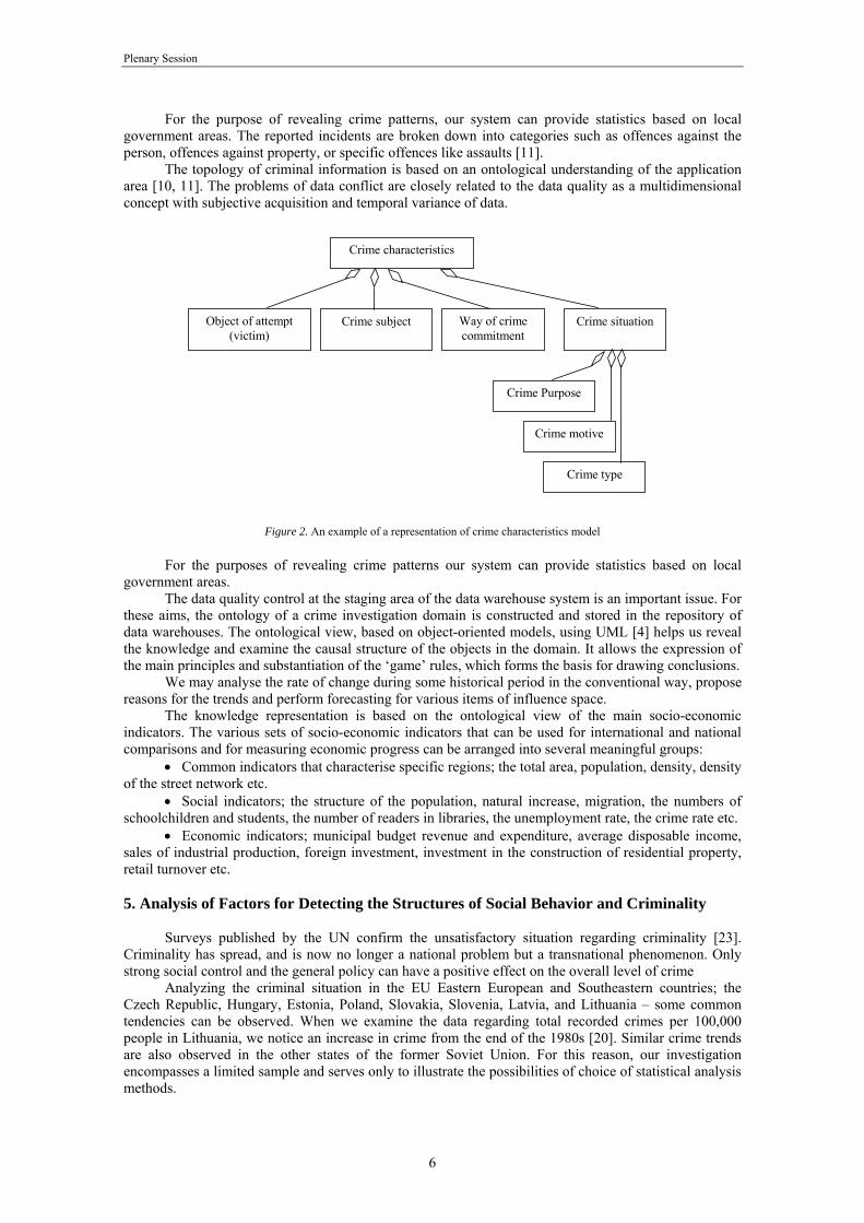
Unified national criminal information systems have been created, based on crime characteristics, which are aggregated and included in DWS as different components. Such components of aggregation space deal with the object of attempt (victim), the crime subject (criminal), the crime situation and the way the crime was committed (Fig. 2).

Plenary Session

6

For the purpose of revealing crime patterns, our system can provide statistics based on local government areas. The reported incidents are broken down into categories such as offences against the person, offences against property, or specific offences like assaults [11].

The topology of criminal information is based on an ontological understanding of the application area [10, 11]. The problems of data conflict are closely related to the data quality as a multidimensional concept with subjective acquisition and temporal variance of data.

Crime characteristics

Object of attempt (victim)

Crime subject Way of crime commitment

Crime situation

Crime Purpose

Crime motive

Crime type

Figure 2. An example of a representation of crime characteristics model

For the purposes of revealing crime patterns our system can provide statistics based on local government areas.

The data quality control at the staging area of the data warehouse system is an important issue. For these aims, the ontology of a crime investigation domain is constructed and stored in the repository of data warehouses. The ontological view, based on object-oriented models, using UML [4] helps us reveal the knowledge and examine the causal structure of the objects in the domain. It allows the expression of the main principles and substantiation of the ‘game’ rules, which forms the basis for drawing conclusions.

We may analyse the rate of change during some historical period in the conventional way, propose reasons for the trends and perform forecasting for various items of influence space.

The knowledge representation is based on the ontological view of the main socio-economic indicators. The various sets of socio-economic indicators that can be used for international and national comparisons and for measuring economic progress can be arranged into several meaningful groups:

• Common indicators that characterise specific regions; the total area, population, density, density of the street network etc.

• Social indicators; the structure of the population, natural increase, migration, the numbers of schoolchildren and students, the number of readers in libraries, the unemployment rate, the crime rate etc.

• Economic indicators; municipal budget revenue and expenditure, average disposable income, sales of industrial production, foreign investment, investment in the construction of residential property, retail turnover etc. 5. Analysis of Factors for Detecting the Structures of Social Behavior and Criminality

Surveys published by the UN confirm the unsatisfactory situation regarding criminality [23]. Criminality has spread, and is now no longer a national problem but a transnational phenomenon. Only strong social control and the general policy can have a positive effect on the overall level of crime

Analyzing the criminal situation in the EU Eastern European and Southeastern countries; the Czech Republic, Hungary, Estonia, Poland, Slovakia, Slovenia, Latvia, and Lithuania – some common tendencies can be observed. When we examine the data regarding total recorded crimes per 100,000 people in Lithuania, we notice an increase in crime from the end of the 1980s [20]. Similar crime trends are also observed in the other states of the former Soviet Union. For this reason, our investigation encompasses a limited sample and serves only to illustrate the possibilities of choice of statistical analysis methods.


7

The crime increase in the Baltic and Eastern European states could be a result of common factors linked to the collapse of the Soviet Union: economic chaos, a lack of economic education and visible property inequalities (rather than the concealed privileges of the Soviet Union). These factors and illegal methods of capital accumulation led to a substantial rise in the crime rate.

The data on total recorded crimes in these countries do not reflect differences between national laws, crime registration systems, or the confidence of citizens in legal institutions. In order to decrease errors caused by these differences, we convert the crime series into dynamic series. Each value of the recorded crimes is translated into a new value, dividing the recorded crimes by the quantity of recorded crimes in 1990 (1):

.11, 1,2,i ,0

…==yyS i

i (1)

To determine the structure of crimes, factor analysis as a classification method was applied.

Applying the factor analysis method, two factors were extracted. The Varimax rotation method of normalized factor loadings [22, p.638] was used for maximizing the variance in the columns of the matrix of squared normalized factor loadings. The correlations between the variables, i.e., factor loadings are presented in Table 1.

Table 1. Normalized factor loadings

Factor Loadings (Varimax normalized) (Marked loadings are > 0.70) Factor 1 Factor 2 Hungary -0.183 0.758Lithuania 0.805 0.524Czech 0.260 0.810Estonia 0.982 0.0830Latvia 0.916 -0.352Poland 0.970 0.027Slovakia -0.683 -0.534Slovenia 0.929 0.201Explained Variance 4.824 1.962

Two factors or two groups of countries were retrieved. Five countries form the first group and two

countries the second one. In order to assess the central tendency of criminality in the first group of states, the arithmetic

mean of the recorded crimes in Lithuania, Estonia, Latvia, Poland, and Slovenia was calculated:

( ) ( )∑=

=k

ii tx

ktx

1.1 (2)

The same calculations were applied to the second group of countries; Hungary and the Czech

Republic. The results are presented in Fig. 4. The geometric mean for both groups has been calculated. For the first group, the average increase

in criminality is 1.41. During the period 1990-2000, in relation to 1990, the increase in criminality in the first group of countries was about 40 percent. For the second group, the geometric mean equals 1.23. So, in the second group the increase was about 20 percent.

Now we can evaluate the average tendencies of crime variation in time, using the regression model.

Since the sample is small, we have used the linear model 1,2,...,11i =++= ,tii xz εβα for the prediction of time series ,3,2,1 , =iz i , which, of

course, does not embrace the whole variety of regression models.

Plenary Session

8

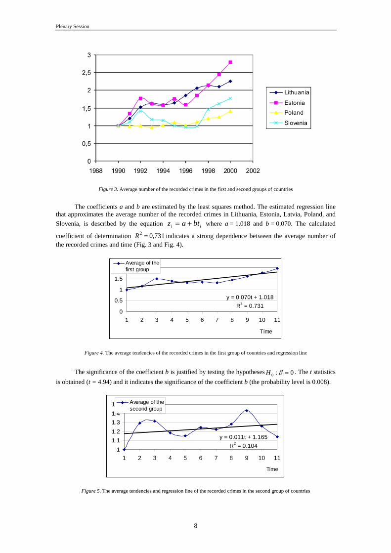
Figure 3. Average number of the recorded crimes in the first and second groups of countries

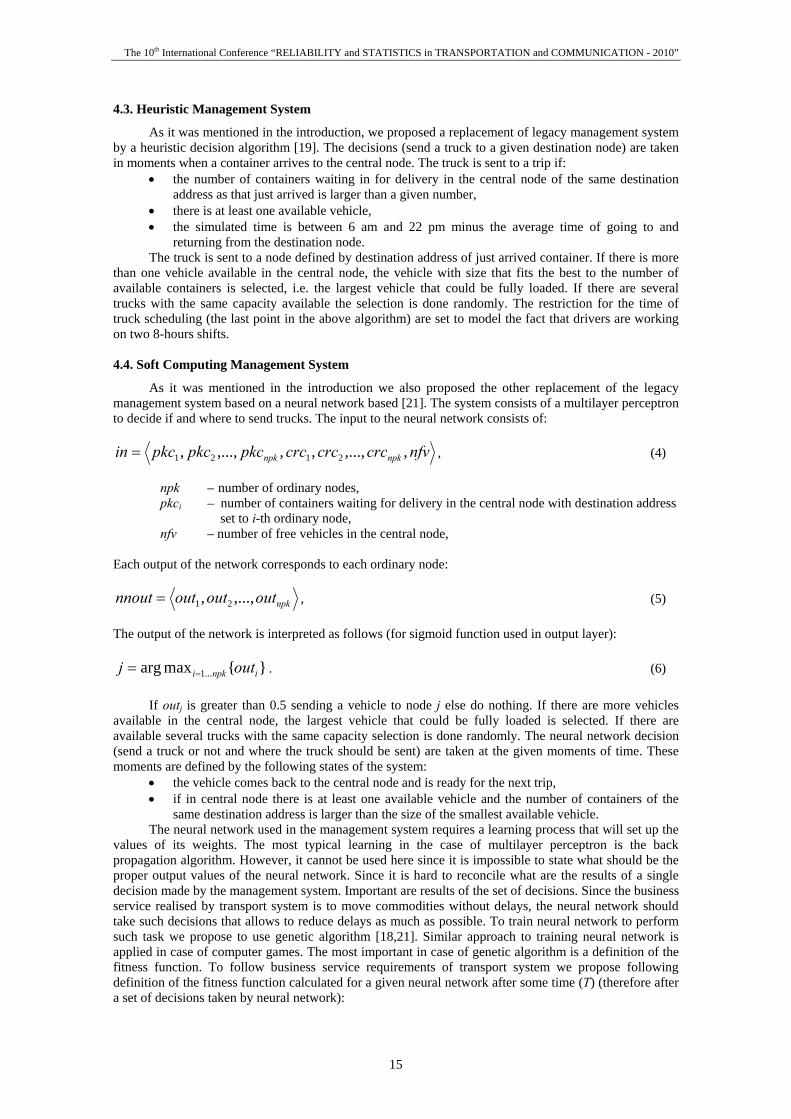
The coefficients a and b are estimated by the least squares method. The estimated regression line

that approximates the average number of the recorded crimes in Lithuania, Estonia, Latvia, Poland, and Slovenia, is described by the equation ii btaz += where a = 1.018 and b = 0.070. The calculated

coefficient of determination 731,02 =R indicates a strong dependence between the average number of the recorded crimes and time (Fig. 3 and Fig. 4).

y = 0.070t + 1.018R2 = 0.731

0

0.5

1

1.5

2

1 2 3 4 5 6 7 8 9 10 11

Time

Average of thefirst group

Figure 4. The average tendencies of the recorded crimes in the first group of countries and regression line

The significance of the coefficient b is justified by testing the hypotheses 0:0 =βH . The t statistics

is obtained (t = 4.94) and it indicates the significance of the coefficient b (the probability level is 0.008).

y = 0.011t + 1.165R2 = 0.1041

1.11.21.31.41.5

1 2 3 4 5 6 7 8 9 10 11

Time

Average of thesecond group

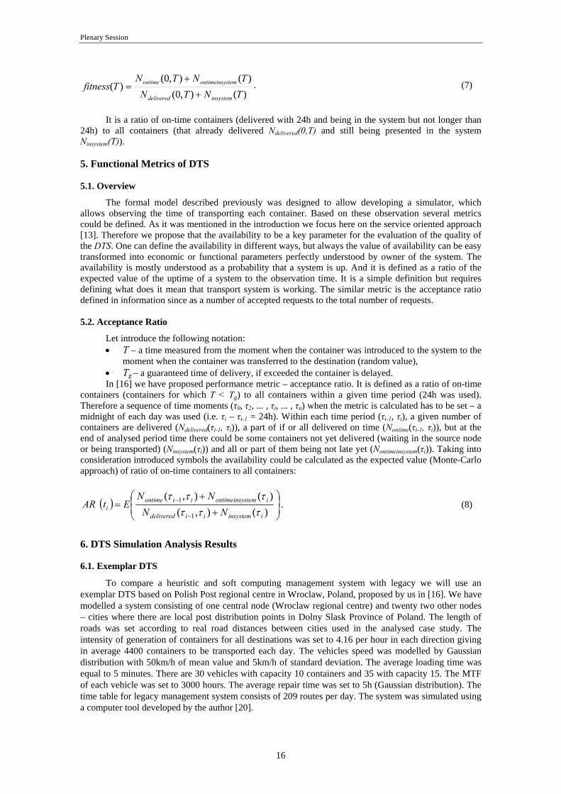
Figure 5. The average tendencies and regression line of the recorded crimes in the second group of countries


9

The approximation of the average number of the recorded crimes in Hungary and the Czech Republic by the regression line is described by the equation ii btaz += where a=1.165 and b=0.011.

The coefficient of determination, in this case, is 104,02 =R (Fig. 5). Because of the low value of the coefficient b and weak correlation, we justify the significance of

the coefficient β. In this case, the t statistic is low (t=1.02) and it indicates that the coefficient b is not significant (the probability level p=0.33). Thus, we can conclude that the correlation between the average tendency of recorded crimes and time is insignificant.

Due to the limited data series, the best model is the linear equation. We should also remember that, due to the short sample, the forecast is not very accurate. However, these equations present the common tendencies of the development of criminal behaviour in two groups of countries.

It would be interesting to examine criminality changes in the same countries during the next decade. To be close to the real situation, such an analysis requires different approaches and probably more complex models, due to additional factors in the process introduced by external events, such as the new states’ joining the EU and the later world economy crisis. 6. Conclusions

A general conceptual framework has been proposed for integrating multiple statistical methods

into the decision support system in order to discover criminal or similar social behavior patterns. The integration of different statistical methods enhances competitive advantages in the analysis of complicated situations and decision-making.

As an example, the criminal situation in the EU Eastern European and Southeastern countries is a way to demonstrate the integration of different methods of statistical analysis to allow the better discovery of patterns and to improve the likelihood of making more correct decisions. An increase in crime was noticed in the states of the former Soviet Union dating from the end of the 1980s. The collected data do not reflect the differences in crime registration systems and the confidence of the citizens in their legal institutions. A dynamic series could decrease errors caused by these differences and isolate the main trends in the rise in crime.

Applying factor analysis methods, two groups of countries were distinguished. The average increase in criminality during the period of 1995-2005 in relation to 1990 in the first group of countries (Lithuania, Estonia, Latvia, Poland, and Slovenia) was about 40% and in the second group (the Czech Republic and Hungary) about 20%. The regression model was applied in evaluating the average tendencies of crime variation in time. The analysis results show that in one group of countries the variation of criminality in time is considerable, while in the other group it is statistically not significant.

The contribution of this paper, we believe, is that it proposes and demonstrates possible methods for estimating social behavior change and integrating them into the semi automatic process of retrieving such methods for decision support and the recognition of relevant patterns. References 1. Aamodt, A. A Knowledge-Intensive, Integrated Approach to Problem Solving and Sustained

Learning. Knowledge Engineering and Image Processing Group. University of Trondheim. 1991, pp.27-85.

2. Asparouhov, T., Muthén, B. Exploratory Structural Equation Modeling. Structural Equation Modeling, A Multidisciplinary Journal, Volume 16 Issue 3, 2009, pp. 397 – 438.

3. Barletta, R. An Introduction to Case-based Reasoning. AI Expert. 1991, pp. 43-49. 4. Booch, G. Object Oriented Analysis and Design with Applications. The Benjamin Cummings

Publishing Co. Inc. Second Edition, 1994. 5. Duncan, J.W., Gross, A.C. Statistics for the 21nt century. Irwin. USA. 1995. 6. Duncan, T. E., Duncan, Susan C., Strycker, Lisa A., Li, Fuzhong, and Alpert, Anthony. An

Introduction to Latent Variable Growth Curve Modeling: Concepts, Issues, and Applications. Mahwah, NJ: Lawrence Erlbaum. 1999.

7. Dzemydiene, D. Consultative Information Systems in Law Domain. Information Technologies and Management. 2001, No.4 (21), p. 38-42.

8. Dzemydiene, D. Intelligent decision support systems for assistance in forensic investigation processes, Handbook of Electronic Security and Digital Forensics / Eds. Hamid Jahankhani, David Lilburn Watson, Gianluigi Me & Frank Leonhardt. Toh Tuck Link: World Scientific Publishing, 2010, p. 603-630.

Plenary Session

10

9. Dzemydienė, D., Rudzkienė, V. Multiple Regression Analysis of Crime Pattern Warehouse for Decision Support. Lecture Note in Computer Science. Vol. 2453. Database and Expert systems Applications. A. Hameurlain, R. Cicchetti, R. Traunmuller (Eds.). Springer. 2002, p.249-258.

10. Dzemydiene, D., Kažemikaitiene, E., Petrauskas, R. Unified Approach of Developing Advisory Information System in Crime Investigation. Databases and Information Systems. H.-M.Haav, A.Kalja (Eds.). In: Proceedings of the Fifth International Baltic Conference. Tallinn. Vol. 2. 2002, p.105-118.

11. Gau, J. M. Basic Principles and Practices of Structural Equation Modeling in Criminal Justice and Criminology Research, Journal of Criminal Justice Education, Volume 21, Issue 2, June 2010, pp. 136 – 151.

12. Herden, O. Parameterized Patterns for Conceptual Modeling of Data Warehouses. In: Proceedings of the 4th IEEE International Baltic Workshop on Databases and Information systems. Technika. Vilnius. 2000, p. 152-163.

13. Hinrichs, H. Statistical quality control of Warehouse Data, Databases and Information Systems. J.Barsdinš, A.Caplinskas (Eds.). Kluwer Academic Publishers. 2001, p.69-84.

14. Kline, R. B. Principles and practice of structural equation modeling. (2nd Edition). New York: The Guilford Press. 2005.

15. Kovacich, G.L, Boni W. High-Technology-Crime Investigator’s Handbook: Working in the Global Information Environment. Butterworth-Heinemann. 2000.

16. Lunejev, V.V. Crime in the XXth century. Moscow, Hopma, 1999 (in Russian). 17. Parsaye, K. Rotational Schemas: Multi-Focus Data Structures for data Mining. Information

Discovery Inc. 1996. 18. Pree, W. Design Patterns for Object-Oriented Software Development. Addison Wesley, 1995. 19. Rudzkiene, V. Mathematical Modeling of Criminality in Lithuania in a Context of the East European

Countries. Liet. Matem. Rink., Vol.41, Spec. No., Vilnius. 2001, p. 548-551 (in Lithuanian). 20. Ullman, J.B. Structural Equation Modeling. Tabachnik, B. G. & Fidell, L. S. Using Multivariate

Statistics (5-th edition). Pearson Education, Inc., pp. 676-780, 2007. 21. Tabachnik, B. G. & Fidell, L. S. Using Multivariate Statistics (5-th edition). Pearson Education, Inc.,

2007. 22. Third to Sixth United Nations Survey on Crime Trends and Operations of Criminal Justice Systems

Combined. URL: http://www.uncjin.org/ 23. Wright S. On the nature of size factors. Genetics, 3, pp. 367-374. 1918.


11

Proceedings of the 10th International Conference “Reliability and Statistics in Transportation and Communication” (RelStat’10), 20–23 October 2010, Riga, Latvia, p. 11-19. ISBN 978-9984-818-34-4 Transport and Telecommunication Institute, Lomonosova 1, LV-1019, Riga, Latvia

DYNAMIC VEHICLE FLEET MANAGEMENT IN DISCRETE TRANSPORT SYSTEMS

Jacek Mazurkiewicz Tomasz Walkowiak

Institute of Computer Engineering, Control and Robotics

Wroclaw University of Technology Janiszewskiego 11/17, 50-372 Wroclaw, Poland

E-mails: [email protected], [email protected]

The paper describes a novel approach to analysis of management algorithms in discrete transport systems (DTS). The proposed method is based on modelling and simulating of the system behaviour. Monte Carlo simulation is a tool for DTS performance metric calculation. No restriction on the system structure and on a kind of distribution is the main advantage of the method. The system is described by the formal model, which includes reliability and functional parameters of DTS. The paper proposes to change the classic time-table based management system of DTS by dynamic heuristic algorithms and algorithms based on artificial neural networks. The paper gives numerical results of simulation experiments. The results allow comparing mentioned above fleet management algorithms in different case studies. Keywords: discrete transport system, reliability, Monte-Carlo simulation, fleet management algorithms, dispatching system 1. Introduction

The serious problem in transport system analysis is to find the suitable methodology for modelling of the management presented in a real system. The performance of the system can be impaired by various types of faults related to the transport vehicles, communication infrastructure or even by traffic congestion [13]. Moreover, it is hard for human (administrator, owner) to understand the system behaviour. To overcome the problems we propose a functional approach. The transport system is analysed from the functional point of view, focusing on business service realised by a system [9]. The analysis is following a classical [4]: modelling and simulation approach. It allows calculating different system measures, which could be a base for decisions related to administration of the transport systems. The metric are calculated using Monte Carlo techniques [7]. No restriction on the system structure and on a kind of distribution is the main advantage of the method. The proposed approach allows forgetting about the classical reliability analysis based on Markov or Semi-Markov processes [2] – idealised and hard for reconciliation with practice. The systems are often driven by a dispatcher – a person who allocates vehicles to the tasks introduced into system. The dispatcher ought to take into account different features which describe the actual situation of all elements of transport systems. The modelling of transport systems with dispatcher is not a trivial challenge. Our previous works [17][18] showed that it is hard to create an "intelligent" algorithm of dispatcher – an algorithm giving significantly better results from pure random algorithms. In this paper we propose a heuristic approach and the neural network based solution to solve this problem. The system is described by the formal model, which includes reliability and functional parameters of transport system. The proposed, novelty approach can serve for practical solving of essential management problems related to an organisation of transport systems. The paper is divided into seventh sections. The second describes Polish Post transport system. The third is focused on dispatcher problem discussion. The possible solutions for dynamic traffic modelling, microscopic model discussion and container manoeuvres problems are presented. Fleet management systems are described in the fourth section. Section number five is focused on definitions of proposed DTS. The next section collects the results. A conclusion we find as the last section. 2. Discrete Transport System - Idea

The analysed transport system is a simplified case of the Polish Post. The business service provided the Polish Post is the delivery of mails. The system consists of a set of nodes placed in different geographical locations. Two kinds of nodes could be distinguished: central nodes (CR) and ordinary nodes (PK). There are bidirectional routes between nodes. Mails are distributed among ordinary nodes by

Plenary Session

12

trucks, whereas between central nodes by trucks, railway or by plain. The mail distribution could be understood by tracing the delivery of some mail from point A to point B. At first the mail is transported to the nearest to A ordinary node. Different mails are collected in ordinary nodes, packed in larger units called containers and then transported by trucks scheduled according to some time-table to the nearest central node. In central node containers are repacked and delivered to appropriate (according to delivery address of each mail) central node. In the Polish Post there are 14 central nodes and more than 300 ordinary nodes. There are more than one million mails going through one central node within 24 hours. It gives a very large system to be modelled and simulated. Therefore, we have decided to model only a part of the Polish Post transport system – one central node with a set of ordinary nodes.

Essential in any system modelling and simulation is to define the level of details of modelled system. Increasing the details causes the simulation becoming useless due to the computational complexity and a large number of required parameter values to be given. On the other hand a high level of modelling could not allow recording required data for system measure calculation. Therefore, the crucial think in the definition of the system level details is to know what kind of measures will be calculated by the simulator. Since the business service given by the post system is the delivery of mails on time. Therefore, we have to calculate the time of transporting mails by the system. Since the number of mails presented in the modelled system is very large and all mails are transported in larger amounts containers, we have decided to use containers as the smallest observable element of the system. Therefore, the main observable value calculated by the simulator will be the time of container transporting from the source to the destination node. The income of mails to the system, or rather containers of mails as it was discussed above, is modelled by a stochastic process. Each container has a source and destination address. The central node is the destination address for all containers generated in the ordinary nodes. Where containers addressed to any ordinary nodes are generated in the central node. The generation of containers is described by some random process. In case of central node, there are separate processes for each ordinary node. Whereas, for ordinary nodes there is one process, since commodities are transported from ordinary nodes to the central node or in the opposite direction. The containers are transported by vehicles. Each vehicle has given capacity – maximum number of containers it can haul. Central node is a base place for all vehicles. They start from the central node and the central node is the destination of their travel. The vehicle hauling a commodity is always fully loaded or taking the last part of the commodity if it is less than its capacity. Vehicles operate according to the time-table. The time-table consists of a set of routes (sequence of nodes starting and ending in the central node, times of leaving each node in the route and the recommended size of a vehicle). The number of used vehicle and the capacity of vehicles do not depend on temporary situation described by number of transportation tasks or by the task amount for example. It means that it is possible to realise the route by completely empty vehicle or the vehicle cannot load the available amount of commodity (the vehicle is too small). Time-table is a fixed element of the system in observable time horizon, but it is possible to use different time-tables for different seasons or months of the year. Summarising the movement of the containers in the system, a container is generated with destination address in some of node (source) at some random time. Next, the container waits in the node for a vehicle to be transported to the destination node. Each day a given time-table is realised, it means that at a time given by the time table a vehicle, selected from vehicles available in the central node, starts from central node and is loaded with containers addressed to each ordinary nodes included in a given route. This is done in a proportional way. When a vehicle approaches the ordinary node it is waiting in an input queue if there is any other vehicle being loaded/unload at the same time. There is only one handling point in each ordinary node. The time of loading/unloading vehicle is described by a random distribution. The containers addressed to given node are unloaded and empty space in the vehicle is filled by containers addressed to a central node. Next, the vehicle waits till the time of leaving the node (set in the time-table) is left and starts its journey to the next node. The operation is repeated in each node on the route and finally the vehicle is approaching the central node when it is fully unloaded and after it is available for the next route. The process of vehicle operation could be stopped at any moment due to a failure (described by a random process). After the failure, the vehicle waits for a maintenance crew (if there are no available due to repairing other vehicles), is being repaired (random time) and after it continues its journey. The vehicle hauling a commodity is always fully loaded or taking the last part of the commodity if it is less than its capacity. 3. Dispatching Problems 3.1. Traffic Modelling Approach

Modelling traffic flow for design, planning and management of transportation systems in urban and highway area has been addressed since the 1950s mostly by the civil engineering community. The


13

following definitions and concepts of traffic simulation modelling can be found in works such as Gartner et al. [8]. Depending on the level of detail in modelling the granularity of traffic flow, traffic models are broadly divided into two categories: macroscopic and microscopic models. According to Gartner et al. [8], a macroscopic model describes the traffic flow as a fluid process with aggregate variables, such as flow and density. The state of the system is then simulated using analytical relationships between average variables such as traffic density, traffic volume, and average speed. On the other hand, a microscopic model reproduces interaction of punctual elements (vehicles, road segments, intersections, etc) in the traffic network. Each vehicle in the system is emulated according to its individual characteristics (length, speed, acceleration, etc.). Traffic is then simulated, using processing logic and models describing vehicle driving behaviour, such as car-following and lane-changing models. Those models reproduce driver-driver and driver-road interactions. Despite its great accuracy level, for many years this highly detailed modelling was considered a computationally intensive approach. Since the last twenty years, with the improvements in processing speed, this microscopic approach becomes more attractive. In fact, Ben-Akiva et al. [3], Barcelo et al. [1] and Liu et al. [12] claim that using microscopic approach is essential to track the real-time traffic state and then, to define strategy to decrease congestion in urban transportation networks. For the control of congestion, they explain that the models must accurately capture the full dynamics of time dependant traffic phenomena and must also track vehicles’ reactions when exposed to Intelligent Transportation Systems (ITS). From the latter assertions, in order to control traffic congestion in internal transportation networks it appears that the microscopic modelling will be more appropriate. A common definition of congestion is the apparition of a delay above the minimum travel time needed to traverse a transportation network. As stated in Taylor et al. [14], this notion is context-specific; and complex because a delay may always appear in dynamic transport system, but this delay must exceed a threshold value in order to be considered. 3.2. Microscopic Model Discussion

Few works have considered the traffic behaviour when studying outdoors vehicle-based internal transport operational problems. In the surface mining environment, pickup and delivery operations involve a fleet of trucks transporting materials from excavation stations to dumping stations, through a designed shared road network. At pickup stations, shovels are continuously digging during a shift according to a pre-assigned mining production plan. Trucks are moving in a cyclical manner between shovels (pickup stations), and dumping areas (delivery stations). A truck cycle time is defined as the time spent by a truck to accomplish an affected mission that consists of travelling to a specific shovel, being serviced by the shovel and hauling material to a specific dumping area. Burt and Caccetta [5] state that mine productivity is very sensitive to truck dispatching decisions which are closely related to the truck cycle time. Thus several papers have studied and proposed algorithms and software to resolve this problematic issue. In fact, this critical decision consists of finding, according to the real environment, to which best shovel a truck must be affected. Such decision has to be generated continuously during a shift, whenever a truck finished dumping at a delivery station. Despite the several proposed dispatching software, recent articles by Krzyzanowska [11] formally criticize the simplistic assumption behind those software which tend to provide dispatching decisions with the objective to optimise a truck cycle times previously calculated. Generally speaking, those software systems based the optimisation process on the past period collected data of trucks cycle times and assume that for the next period trucks will spend on average the same time to accomplish missions. But in the reality of mining operation, the duration of truck travel time appears to be very sensitive to the variable traffic state and road conditions. Burt and Caccetta [5] and Krzyzanowska [11], point out the unresolved problematic of truck bunching and platoon formation in mining road network which apparently induce lower productivity. 3.3. Container Manoeuvres

Similarly to material transportation in mining operation, several papers (Ioannou [10], Vis [15]) have provided methods for improving container terminal complex operations. In such applications, three types of handling operations are defined: vessel operations, receiving/delivery operations and container handling and storage operations in the stack yards. As we are interested by internal transportation systems, our review concerns the papers dealing with the container handling and storage operations in the stack yards. Generally speaking, vessels bring inbound containers to be picked up by internal trucks and distributed to the respective stocks in the yard. Once discharged, vessels have to leave with on board outbound containers which also are delivered by internal trucks from the storage yard. For this purpose, trucks are moving through a terminal internal road network. In order to decrease the vessel turnaround time, which is the most important performance measure of container terminals, it is important to perform

Plenary Session

14

those operations as quickly as possible. In fact according to [3], this movement of containers between quay sides and storage yards appears to greatly affect the productivity of containership’s journey. Vis and Koster [15] gives an extended review of numerous research papers, providing algorithms to solve this complex routing and scheduling problem. They criticize the lack of consistency of the simplistic assumptions made to solve the proposed models within the real-world highly stochastic environment. The ignored traffic situation in the complex seaport internal transportation network is strongly criticized in recent papers [4], [10]. For example, in [3], a travel time of a container internal truck is modelled as a static mean time of travel, based on the distance and the truck average speed. Duinkerken et al. [6], put a uniform distribution between zero and 30% of the nominal travel time formulation, aiming to assimilate the complexity of traffic. More accurate work to solve this issue is the one provided recently by Liu, Chu and Recker [12]. They integrate a traffic model to the internal service model and reported the effectiveness of this integration which allows analysing the tractor traffic flow in a port container terminal. Conscious about the critical problem of congestion in the road network inside a terminal, a quantitative measure of congestion to be added as a controllable decision variable had been developed. For this purpose, they considered the road system inside the terminal as a directed network and they measured flows on arcs in units of trucks travelling per unit time. Those two last works appear as providing the leader approach in term of consideration of congestion and traffic in container terminals; however, their approach is ultimately macroscopic. As we have lately discussed, even if this macroscopic approach allows analysing the traffic behaviour, the highly detailed microscopic model is more efficient for an effective real-time traffic monitoring and control. 4. Fleet Management Systems 4.1. Discrete Transport System Formal Model

The described in the section two regional part of the Polish Post transport system with one central node and several ordinary nodes was a base for a formal model definition of the discrete transport system with central node (DTS). Users generate tasks, which are being realised by the system. The task to be realised requires some services available in the system. A realisation of the service needs a defined set of technical resources. Moreover, the vehicles transporting mails between system nodes are steering by the management system. Therefore, we can model discrete transport system as a quadruple [18, 20]:

,,,, MSTIBSClientDTS = (1)

Client – client model, BS – business service, a finite set of service components, TI – technical infrastructure, MS – management system.

4.2. Legacy Management System

The management system (MS) of the DTS controls the operation of vehicle. It consists of a sequence of routes:

nrrrrMS ,...,, 21= . (2)

Each route is a sequence of nodes starting and ending in the central node, times of leaving each node in the route (ti) and the recommended size of a vehicle (size):

{ } htttCRNovsizeCRtntntCRr mimm 24...0,,,,...,,,, 10110 <<<<≤−∈= . (3)

The routes are defined for one day and are repeated each day. The management system selects vehicles to realise each route in random way, first of all vehicles (among vehicles available in central node) with capacity equal to recommended size are taken into consideration. If there is no such vehicle, vehicles with larger capacity are taken into consideration. If still there is no vehicle fulfilling requirements vehicle of smaller size is randomly selected. If there is no available vehicle a given route is not realised.


15

4.3. Heuristic Management System

As it was mentioned in the introduction, we proposed a replacement of legacy management system by a heuristic decision algorithm [19]. The decisions (send a truck to a given destination node) are taken in moments when a container arrives to the central node. The truck is sent to a trip if:

• the number of containers waiting in for delivery in the central node of the same destination address as that just arrived is larger than a given number,

• there is at least one available vehicle, • the simulated time is between 6 am and 22 pm minus the average time of going to and

returning from the destination node. The truck is sent to a node defined by destination address of just arrived container. If there is more

than one vehicle available in the central node, the vehicle with size that fits the best to the number of available containers is selected, i.e. the largest vehicle that could be fully loaded. If there are several trucks with the same capacity available the selection is done randomly. The restriction for the time of truck scheduling (the last point in the above algorithm) are set to model the fact that drivers are working on two 8-hours shifts. 4.4. Soft Computing Management System

As it was mentioned in the introduction we also proposed the other replacement of the legacy management system based on a neural network based [21]. The system consists of a multilayer perceptron to decide if and where to send trucks. The input to the neural network consists of:

nfvcrccrccrcpkcpkcpkcin npknpk ,,...,,,,...,, 2121= , (4) npk – number of ordinary nodes, pkci – number of containers waiting for delivery in the central node with destination address

set to i-th ordinary node, nfv – number of free vehicles in the central node, Each output of the network corresponds to each ordinary node:

npkoutoutoutnnout ,...,, 21= , (5) The output of the network is interpreted as follows (for sigmoid function used in output layer):

}{maxarg ...1 inpki outj == . (6)

If outj is greater than 0.5 sending a vehicle to node j else do nothing. If there are more vehicles available in the central node, the largest vehicle that could be fully loaded is selected. If there are available several trucks with the same capacity selection is done randomly. The neural network decision (send a truck or not and where the truck should be sent) are taken at the given moments of time. These moments are defined by the following states of the system:

• the vehicle comes back to the central node and is ready for the next trip, • if in central node there is at least one available vehicle and the number of containers of the

same destination address is larger than the size of the smallest available vehicle. The neural network used in the management system requires a learning process that will set up the

values of its weights. The most typical learning in the case of multilayer perceptron is the back propagation algorithm. However, it cannot be used here since it is impossible to state what should be the proper output values of the neural network. Since it is hard to reconcile what are the results of a single decision made by the management system. Important are results of the set of decisions. Since the business service realised by transport system is to move commodities without delays, the neural network should take such decisions that allows to reduce delays as much as possible. To train neural network to perform such task we propose to use genetic algorithm [18,21]. Similar approach to training neural network is applied in case of computer games. The most important in case of genetic algorithm is a definition of the fitness function. To follow business service requirements of transport system we propose following definition of the fitness function calculated for a given neural network after some time (T) (therefore after a set of decisions taken by neural network):

Plenary Session

16

)(),0()(),0(

)(TNTNTNTN

Tfitnessinsystemdelivered

stemontimeinsyontime

+

+= . (7)

It is a ratio of on-time containers (delivered with 24h and being in the system but not longer than

24h) to all containers (that already delivered Ndelivered(0,T) and still being presented in the system Ninsystem(T)). 5. Functional Metrics of DTS 5.1. Overview

The formal model described previously was designed to allow developing a simulator, which allows observing the time of transporting each container. Based on these observation several metrics could be defined. As it was mentioned in the introduction we focus here on the service oriented approach [13]. Therefore we propose that the availability to be a key parameter for the evaluation of the quality of the DTS. One can define the availability in different ways, but always the value of availability can be easy transformed into economic or functional parameters perfectly understood by owner of the system. The availability is mostly understood as a probability that a system is up. And it is defined as a ratio of the expected value of the uptime of a system to the observation time. It is a simple definition but requires defining what does it mean that transport system is working. The similar metric is the acceptance ratio defined in information since as a number of accepted requests to the total number of requests. 5.2. Acceptance Ratio

Let introduce the following notation: • T – a time measured from the moment when the container was introduced to the system to the

moment when the container was transferred to the destination (random value), • Tg – a guaranteed time of delivery, if exceeded the container is delayed. In [16] we have proposed performance metric – acceptance ratio. It is defined as a ratio of on-time

containers (containers for which T < Tg) to all containers within a given time period (24h was used). Therefore a sequence of time moments (τ0, τ2, ... , τi, ... , τn) when the metric is calculated has to be set – a midnight of each day was used (i.e. τi – τi-1 = 24h). Within each time period (τi-1, τi), a given number of containers are delivered (Ndelivered(τi-1, τi)), a part of if or all delivered on time (Nontime(τi-1, τi)), but at the end of analysed period time there could be some containers not yet delivered (waiting in the source node or being transported) (Ninsystem(τi)) and all or part of them being not late yet (Nontimeinsystem(τi)). Taking into consideration introduced symbols the availability could be calculated as the expected value (Monte-Carlo approach) of ratio of on-time containers to all containers:

( ) ⎟⎟⎠

⎞⎜⎜⎝

⎛

+

+=

−

−

)(),()(),(

1

1

iinsystemiidelivered

istemontimeinsyiiontimei NN

NNEtAR

ττττττ

. (8)

6. DTS Simulation Analysis Results 6.1. Exemplar DTS

To compare a heuristic and soft computing management system with legacy we will use an exemplar DTS based on Polish Post regional centre in Wroclaw, Poland, proposed by us in [16]. We have modelled a system consisting of one central node (Wroclaw regional centre) and twenty two other nodes – cities where there are local post distribution points in Dolny Slask Province of Poland. The length of roads was set according to real road distances between cities used in the analysed case study. The intensity of generation of containers for all destinations was set to 4.16 per hour in each direction giving in average 4400 containers to be transported each day. The vehicles speed was modelled by Gaussian distribution with 50km/h of mean value and 5km/h of standard deviation. The average loading time was equal to 5 minutes. There are 30 vehicles with capacity 10 containers and 35 with capacity 15. The MTF of each vehicle was set to 3000 hours. The average repair time was set to 5h (Gaussian distribution). The time table for legacy management system consists of 209 routes per day. The system was simulated using a computer tool developed by the author [20].


17

6.2. Calculated Results for Critical Situations

All three presented management algorithms give acceptance ratio almost equal 1 for presented system. To compare these algorithms more deeply we propose to analyse the transport system performance in case of some critical situations [16]. Let’s assume that for some days the system is working at 50%. The tie-up of the system could be caused for example by a drivers’ strike or some contagious diseases resulting in situation that only 50% of vehicles are in operation. After a given number of days the system is again fully working. The achieved results (acceptance ratio calculated according to (8)) for 4 and 14 days tie-up are presented on Figure 1a and 1b. As it could be expected the acceptance ratio in day 10 (when critical situation starts) is starting to drop down and when drivers come back is enlarging. However the system with heuristic management as well as with soft computing one is coming back to normal operation much faster than legacy one. The soft computing one is slightly outperforming the heuristic one.

Next, we have analysed the ability of each management system to return the DTS to normal performance after critical situation of different duration. Results are presented in Figure 2. As it could be seen soft computing and heuristic algorithm give almost identical results, which significantly out performance the legacy management system. a)

b)

Figure 1. Acceptance ratio for 4 days (a) and 14 days (b) tie-up vehicles for legacy, heuristic and soft computing management system

Plenary Session

18

Figure 2. Time of returning DTS performance (measured by acceptance ratio) to 0.95 of normal performance after a critical sitauation (tie-up) ocuurance for legacy, heuristic and soft computing management system

7. Conclusions

We have presented an approach to analyse management algorithms of discrete transport system (DTS) by modelling and simulation. The DTS model was simulated using developed by the authors’ simulation software. We have compared three different management algorithms: legacy one (based on real time-table management in Post system), heuristic and soft computing one. The presented results show that soft computing management system allows the DTS to return to normal operation after some critical situation in the shortest time. The results for heuristic management system are very close to soft computing approach, whereas, the legacy system is performing much worse. Since the soft computing algorithm requires a time consuming learning procedure we propose to use in practice much simpler heuristic management system. The performance of heuristic solution (measured as the time of returning DTS to normal work) is only slightly worse than available by soft computing approach. The achieved simulation results look promising. We hope that it could be implemented in real transport system.

Work reported in this paper was sponsored by a grant No N N509 496238, (years: 2010-2013) from the Polish Ministry of Science and Higher Education. References 1. Barcelo, J., Codina, E., Casas, J., Ferrer, J.L. and Garcia, D. Microscopic Traffic Simulation: a Tool

for the Design, Analysis And Evaluation Of Intelligent Transport Systems, Journal of Intelligent and Robotic Systems: Theory and Applications, Vol. 41, 2005, pp. 173-203.

2. Barlow, R. and Proschan, F . Mathematical Theory of Reliability. Philadelphia: Society for Industrial and Applied Mathematics, 1996. 345 p.

3. Ben-Akiva, M., Cuneo, D., Hasan, M., Jha, M. and Yang, Q. Evaluation of Freeway Control Using a Microscopic Simulation Laboratory, Transportation Research, Part C (Emerging Technologies), Vol. 11C, 2003, pp. 29-50.

4. Birta, L. and Arbez, G. Modelling and Simulation: Exploring Dynamic System Behaviour. London: Springer, 2007. 246 p.

5. Burt, C.N. and Caccetta, L. Match Factor for Heterogeneous Truck and Loader Fleets, International Journal of Mining, Reclamation and Environment, Vol. 21, 2007, pp. 262-270.

6. Duinkerken, M.B., Dekker, R., Kurstjens, S.T.G.L., Ottjes, J.A., and Dellaert, N.P. Comparing Transportation Systems for Inter-Terminal Transport at the Maasvlakte Container Terminals, OR Spectrum, Vol. 28, 2006, pp. 469-493.


19

7. Fishman, G. Monte Carlo: Concepts, Algorithms, and Applications. Springer-Verlag, 1996. 129 p. 8. Gartner, N., Messer, C.J. and Rathi, A.K. Traffic Flow Theory and Characteristics. In: T.R. Board

(Ed.). Texas: University of Texas at Austin, 1998. 125 p. 9. Gold, N., Knight, C., Mohan, A. and Munro, M. Understanding service-oriented software, IEEE

Software, Vol. 21, 2004, pp. 71-77. 10. Ioannou, P.A. Intelligent Freight Transportation. Carolina: Taylor and Francis Group, 2008. 245 p. 11. Krzyzanowska, J. The Impact of Mixed Fleet Hauling on Mining Operations at Venetia Mine,

Journal of The South African Institute of Mining and Metallurgy, Vol. 107, 2007, pp. 215-224. 12. Liu, H., Chu, L. and Recker, W. Performance Evaluation of ITS Strategies Using Microscopic

Simulation. In: Proceedings of the 7th International IEEE Conference on Intelligent Transportation Systems, 2004, pp. 255-270.

13. Sanso, B. and Milot, L. Performability of a Congested Urban-Transportation Network when Accident Information is Available, Transportation Science, Vol. 33, No 1, 1999, pp. 10-21.

14. Taylor, M.A.P., Woolley, J.E. and Zito, R. Integration of the Global Positioning System and Geographical Information Systems for Traffic Congestion Studies, Transportation Research, Part C (Emerging Technologies), Vol. 8C, 2000, pp. 257-285.

15. Vis, I.F.A. Survey of Research in the Design and Control of Automated Guided Vehicle Systems, European Journal of Operational Research, Vol. 170, 2006, pp. 677-709.

16. Walkowiak, T. and Mazurkiewicz, J. Analysis of Critical Situations in Discrete Transport Systems. In : Proceedings of International Conference on Dependability of Computer Systems, Brunow, Poland, June 30-July 2, 2009. Los Alamitos: IEEE Computer Society Press, 2009, pp. 364-371.

17. Walkowiak, T. and Mazurkiewicz, J. Availability of Discrete Transport System Simulated by SSF Tool. In: Proceedings of International Conference on Dependability of Computer Systems, Szklarska Poreba, Poland, June, 2008. Los Alamitos: IEEE Computer Society Press, 2008, pp. 430-437.

18. Walkowiak, T. and Mazurkiewicz, J. Functional Availability Analysis of Discrete Transport System Realized by SSF Simulator. In: Computational Science – ICCS 2008, 8th International Conference, Krakow, Poland, June 2008. Springer-Verlag, LNCS 5101, 2008. Part I, pp. 671-678.

19. Walkowiak, T. and Mazurkiewicz, J. Algorithmic Approach to Vehicle Dispatching in Discrete Transport Systems. In: Technical approach to dependability / Ed. by Jarosław Sugier, et al. Wroclaw: Oficyna Wydawnicza Politechniki Wroclawskiej, 2010. pp. 173-188.

20. Walkowiak, T. and Mazurkiewicz, J. Functional Availability Analysis of Discrete Transport System Simulated by SSF Tool, International Journal of Critical Computer-Based Systems, Vol. 1, No 1-3, 2010, pp. 255-266.

21. Walkowiak, T. and Mazurkiewicz, J. Soft Computing Approach to Discrete Transport System Management. In: Lecture Notes in Computer Science. Lecture Notes in Artificial Intelligence. Springer-Verlag, 2010. Vol. 6114, pp. 675-682.

pattern recognition based on statistics and … · not easy to extract relevant patterns from a...

Documents