mark d reckase multidimensional item response theory (statistics for social and behavioral sciences)...
TRANSCRIPT


Statistics for Social and Behavioral Sciences
Advisors:
S.E. FienbergW.J. van der Linden
For other titles published in this series, go tohttp://www.springer.com/3463

Mark D. Reckase
Multidimensional ItemResponse Theory
123

Mark D. ReckaseMichigan State UniversityCounseling, Educational, Psychology,
and Special Education Department461 Erickson HallEast Lansing MI 48824-1034USA
MATLAB R© is the registered trademark of The MathWorks, Inc.
ISBN 978-0-387-89975-6 e-ISBN 978-0-387-89976-3DOI 10.1007/978-0-387-89976-3Springer Dordrecht Heidelberg London New York
Library of Congress Control Number: 2009927904
c© Springer Science+Business Media, LLC 2009All rights reserved. This work may not be translated or copied in whole or in part without the writtenpermission of the publisher (Springer Science+Business Media, LLC, 233 Spring Street, New York,NY 10013, USA), except for brief excerpts in connection with reviews or scholarly analysis. Use inconnection with any form of information storage and retrieval, electronic adaptation, computer software,or by similar or dissimilar methodology now known or hereafter developed is forbidden.The use in this publication of trade names, trademarks, service marks, and similar terms, even if they arenot identified as such, is not to be taken as an expression of opinion as to whether or not they are subjectto proprietary rights.
Printed on acid-free paper
Springer is part of Springer Science+Business Media (www.springer.com)

Preface
Item response theory (IRT) is a general framework for specifying mathematicalfunctions that describe the interactions of persons and test items. It has a longhistory, but its popularity is generally attributed to the work of Fredrick Lord andGeorg Rasch starting in the 1950s and 1960s. Multidimensional item response the-ory (MIRT) is a special case of IRT that is built on the premise that the mathematicalfunction includes as parameters a vector of multiple person characteristics that de-scribe the skills and knowledge that the person brings to a test and a vector of itemcharacteristics that describes the difficulty of the test item and the sensitivity of thetest item to differences in the characteristics of the persons. MIRT also has a longhistory, going back to the work of Darrel Bock, Paul Horst, Roderick McDonald,Bengt Muthen, Fumiko Samajima, and others starting in the 1970s.
The goal of this book is to draw together in one place the developments in thearea of MIRT that have occurred up until 2008. Of course, it is not possible to betotally comprehensive, but it is believed that most of the major developments havebeen included.
The book is organized into three major parts. The first three chapters give back-ground information that is useful for the understanding of MIRT. Chapter 1 is ageneral conceptual overview. Chapter 2 provides a summary of unidimensional IRT.Chapter 3 provides a summary of the historical underpinnings of MIRT. Chapter 2can be skipped if the reader already has familiarity with IRT. Chapter 3 providesuseful background, but it is not required for understanding of the later chapters.
The second part of the book includes Chaps. 4–6. These chapters describe thebasic characteristics of MIRT models. Chapter 4 describes the mathematical formsof the models. Chapter 5 summarizes the statistics that are used to describe the waythat test items function within an MIRT context. Chapter 6 describes procedures forestimating the parameters for the models.
The third part of the book provides information needed to apply the models andgives some examples of applications. Chapter 7 addresses the number of dimensionsneeded to describe the interactions between persons and test items. Chapter 8 showshow to define the coordinate system that is used to locate persons in a space relativeto the constructs defined by the test items. Chapter 9 describes methods for convert-ing parameter estimates from different MIRT calibrations to the same coordinatesystem. Finally, Chap. 10 shows how all of these procedures can be applied in thecontext of computerized adaptive testing.
v

vi Preface
Chapters 4–9 have been used for a graduate level course in MIRT. In the contextof such a course, Chap. 10 can be used as an example of the application of themethodology. The early chapters of the book are a review of basic concepts thatadvanced graduate students should know, but that need to be refreshed.
Chapters 7–9 should be particularly useful for those who are interested inusing MIRT for the analysis and reporting of large-scale assessment results.Those chapters lay out the procedures for specifying a multidimensional coor-dinate space and for converting results from subsequent calibrations of test formsto that same coordinate system. These are procedures that are needed to maintaina large-scale assessment system over years. The content of these chapters alsoaddresses methods for reporting subscores using MIRT.
There are many individuals that deserve some credit for the existence of thisbook. First, my wife, Char Reckase, did heroic labors proofing the first drafts ofthe full manuscript. This is second only to the work she did typing my dissertationback in the days before personal computers. Second, the members of the STARDepartment at ACT, Inc. helped with a lot of the early planning of this book. TerryAckerman, Jim Carlson, Tim Davey, Ric Leucht, Tim Miller, Judy Spray, and TonyThompson were all part of that group and did work on MIRT. Several of them evenagreed to write chapters for an early version of the book – a few even finished firstdrafts. Although I profited from all of that work, I decided to start over again severalyears ago because there had been a substantial increase in new research on MIRT.
The third contributors to the book were the graduate students who reacted tofirst drafts of the chapters as part of my graduate courses in IRT and an advancedseminar in MIRT. Many students contributed and there are too many to list here.However, Young Yee Kim, Adam Wyse, and Raymond Mapuranga provided muchmore detailed comments than others and need to be honored for that contribution.
East Lansing, MI M.D. Reckase
Contents
1 Introduction . . . . . . . . . . . . . . . . . . . . . . . . . . . . . . . . . . . . . . . . . . . . . . . . . . . . . . . . . . . . . . . . . . . . 11.1 A Conceptual Framework for Thinking About People
and Test Items. . . . . . . . . . . . . . . . . . . . . . . . . . . . . . . . . . . . . . . . . . . . . . . . . . . . . . . . . . . . . 31.2 General Assumptions Behind Model Development .. . . . . . . . . . . . . . . . . . . . 81.3 Exercises . . . . . . . . . . . . . . . . . . . . . . . . . . . . . . . . . . . . . . . . . . . . . . . . . . . . . . . . . . . . . . . . . . 10
2 Unidimensional Item Response Theory Models . . . . . . . . . . . . . . . . . . . . . . . . . . . . 112.1 Unidimensional Models of the Interactions of Persons
and Test Items. . . . . . . . . . . . . . . . . . . . . . . . . . . . . . . . . . . . . . . . . . . . . . . . . . . . . . . . . . . . . 112.1.1 Models for Items with Two Score Categories. . . . . . . . . . . . . . . . . . . 142.1.2 Relationships Between UIRT Parameters
and Classical Item Statistics . . . . . . . . . . . . . . . . . . . . . . . . . . . . . . . . . . . . . 262.1.3 Models for Items with More Than Two Score Categories . . . . . 32
2.2 Other Descriptive Statistics for Items and Tests. . . . . . . . . . . . . . . . . . . . . . . . . 432.2.1 The Test Characteristic Curve . . . . . . . . . . . . . . . . . . . . . . . . . . . . . . . . . . . 432.2.2 Information Function . . . . . . . . . . . . . . . . . . . . . . . . . . . . . . . . . . . . . . . . . . . . 47
2.3 Limitations of Unidimensional IRT Models. . . . . . . . . . . . . . . . . . . . . . . . . . . . . 532.4 Exercises . . . . . . . . . . . . . . . . . . . . . . . . . . . . . . . . . . . . . . . . . . . . . . . . . . . . . . . . . . . . . . . . . . 54
3 Historical Background for Multidimensional ItemResponse Theory . . . . . . . . . . . . . . . . . . . . . . . . . . . . . . . . . . . . . . . . . . . . . . . . . . . . . . . . . . . . . . . 573.1 Psychological and Educational Context for MIRT .. . . . . . . . . . . . . . . . . . . . . 603.2 Test Development Context for MIRT . . . . . . . . . . . . . . . . . . . . . . . . . . . . . . . . . . . . 613.3 Psychometric Antecedents of MIRT . . . . . . . . . . . . . . . . . . . . . . . . . . . . . . . . . . . . . 63
3.3.1 Factor Analysis . . . . . . . . . . . . . . . . . . . . . . . . . . . . . . . . . . . . . . . . . . . . . . . . . . . 633.3.2 Item Response Theory . . . . . . . . . . . . . . . . . . . . . . . . . . . . . . . . . . . . . . . . . . . 683.3.3 Comparison of the Factor Analytic and MIRT Approaches .. . . 70
3.4 Early MIRT Developments .. . . . . . . . . . . . . . . . . . . . . . . . . . . . . . . . . . . . . . . . . . . . . . 713.5 Developing Applications of MIRT. . . . . . . . . . . . . . . . . . . . . . . . . . . . . . . . . . . . . . . 743.6 Influence of MIRT on the Concept of a Test . . . . . . . . . . . . . . . . . . . . . . . . . . . . 753.7 Exercises . . . . . . . . . . . . . . . . . . . . . . . . . . . . . . . . . . . . . . . . . . . . . . . . . . . . . . . . . . . . . . . . . . 76
vii
viii Contents
4 Multidimensional Item Response Theory Models . . . . . . . . . . . . . . . . . . . . . . . . . 794.1 Multidimensional Models for the Interaction Between
a Person and a Test Item.. . . . . . . . . . . . . . . . . . . . . . . . . . . . . . . . . . . . . . . . . . . . . . . . . 854.1.1 MIRT Models for Test Items with Two Score Categories . . . . . . 854.1.2 MIRT Models for Test Items with More Than
Two Score Categories . . . . . . . . . . . . . . . . . . . . . . . . . . . . . . . . . . . . . . . . . . . . 1024.2 Future Directions for Model Development .. . . . . . . . . . . . . . . . . . . . . . . . . . . . . 1104.3 Exercises . . . . . . . . . . . . . . . . . . . . . . . . . . . . . . . . . . . . . . . . . . . . . . . . . . . . . . . . . . . . . . . . . . 111
5 Statistical Descriptions of Item and Test Functioning . . . . . . . . . . . . . . . . . . . . . 1135.1 Item Difficulty and Discrimination . . . . . . . . . . . . . . . . . . . . . . . . . . . . . . . . . . . . . . 1135.2 Item Information .. . . . . . . . . . . . . . . . . . . . . . . . . . . . . . . . . . . . . . . . . . . . . . . . . . . . . . . . . 1215.3 MIRT Descriptions of Test Functioning .. . . . . . . . . . . . . . . . . . . . . . . . . . . . . . . . 1245.4 Summary and Conclusions .. . . . . . . . . . . . . . . . . . . . . . . . . . . . . . . . . . . . . . . . . . . . . . 1335.5 Exercises . . . . . . . . . . . . . . . . . . . . . . . . . . . . . . . . . . . . . . . . . . . . . . . . . . . . . . . . . . . . . . . . . . 134
6 Estimation of Item and Person Parameters . . . . . . . . . . . . . . . . . . . . . . . . . . . . . . . . 1376.1 Background Concepts for Parameter Estimation . . . . . . . . . . . . . . . . . . . . . . . . 138
6.1.1 Estimation of the ™-vector with Item Parameters Known . . . . . . 1386.2 Computer Programs for Estimating MIRT Parameters . . . . . . . . . . . . . . . . . 148
6.2.1 TESTFACT .. . . . . . . . . . . . . . . . . . . . . . . . . . . . . . . . . . . . . . . . . . . . . . . . . . . . . . 1496.2.2 NOHARM .. . . . . . . . . . . . . . . . . . . . . . . . . . . . . . . . . . . . . . . . . . . . . . . . . . . . . . . 1586.2.3 ConQuest . . . . . . . . . . . . . . . . . . . . . . . . . . . . . . . . . . . . . . . . . . . . . . . . . . . . . . . . . 1626.2.4 BMIRT. . . . . . . . . . . . . . . . . . . . . . . . . . . . . . . . . . . . . . . . . . . . . . . . . . . . . . . . . . . . 168
6.3 Comparison of Estimation Programs . . . . . . . . . . . . . . . . . . . . . . . . . . . . . . . . . . . . 1756.4 Exercises . . . . . . . . . . . . . . . . . . . . . . . . . . . . . . . . . . . . . . . . . . . . . . . . . . . . . . . . . . . . . . . . . . 176
7 Analyzing the Structure of Test Data . . . . . . . . . . . . . . . . . . . . . . . . . . . . . . . . . . . . . . . . 1797.1 Determining the Number of Dimensions for an Analysis . . . . . . . . . . . . . . 179
7.1.1 Over and Under-Specification of Dimensions . . . . . . . . . . . . . . . . . . 1817.1.2 Theoretical Requirements for Fit
by a One-Dimensional Model . . . . . . . . . . . . . . . . . . . . . . . . . . . . . . . . . . . 1947.2 Procedures for Determining the Required Number of Dimensions . . . . 201
7.2.1 DIMTEST . . . . . . . . . . . . . . . . . . . . . . . . . . . . . . . . . . . . . . . . . . . . . . . . . . . . . . . . 2087.2.2 DETECT.. . . . . . . . . . . . . . . . . . . . . . . . . . . . . . . . . . . . . . . . . . . . . . . . . . . . . . . . . 2117.2.3 Parallel Analysis . . . . . . . . . . . . . . . . . . . . . . . . . . . . . . . . . . . . . . . . . . . . . . . . . 2157.2.4 Difference Chi-Square . . . . . . . . . . . . . . . . . . . . . . . . . . . . . . . . . . . . . . . . . . . 218
7.3 Clustering Items to Confirm Dimensional Structure .. . . . . . . . . . . . . . . . . . . 2207.4 Confirmatory Analysis to Check Dimensionality . . . . . . . . . . . . . . . . . . . . . . . 2247.5 Concluding Remarks . . . . . . . . . . . . . . . . . . . . . . . . . . . . . . . . . . . . . . . . . . . . . . . . . . . . . 2287.6 Exercises . . . . . . . . . . . . . . . . . . . . . . . . . . . . . . . . . . . . . . . . . . . . . . . . . . . . . . . . . . . . . . . . . . 229

Contents ix
8 Transforming Parameter Estimates to a SpecifiedCoordinate System . . . . . . . . . . . . . . . . . . . . . . . . . . . . . . . . . . . . . . . . . . . . . . . . . . . . . . . . . . . . 2338.1 Converting Parameters from One Coordinate System to Another . . . . . . 235
8.1.1 Translation of the Origin of the ™-Space . . . . . . . . . . . . . . . . . . . . . . . . 2398.1.2 Rotating the Coordinate Axes of the ™-Space . . . . . . . . . . . . . . . . . . 2448.1.3 Changing the Units of the Coordinate Axes . . . . . . . . . . . . . . . . . . . . 2528.1.4 Converting Parameters Using Translation,
Rotation, and Change of Units . . . . . . . . . . . . . . . . . . . . . . . . . . . . . . . . . . 2578.2 Recovering Transformations from Item- and Person-Parameters . . . . . . 261
8.2.1 Recovering Transformations from ™-vectors . . . . . . . . . . . . . . . . . . . 2628.2.2 Recovering Transformations Using Item Parameters . . . . . . . . . . . 266
8.3 Transforming the ™-space for the Partially Compensatory Model . . . . . 2698.4 Exercises . . . . . . . . . . . . . . . . . . . . . . . . . . . . . . . . . . . . . . . . . . . . . . . . . . . . . . . . . . . . . . . . . . 271
9 Linking and Scaling . . . . . . . . . . . . . . . . . . . . . . . . . . . . . . . . . . . . . . . . . . . . . . . . . . . . . . . . . . . 2759.1 Specifying the Common Multidimensional Space . . . . . . . . . . . . . . . . . . . . . . 2769.2 Relating Results from Different Test Forms. . . . . . . . . . . . . . . . . . . . . . . . . . . . . 286
9.2.1 Common-Person Design . . . . . . . . . . . . . . . . . . . . . . . . . . . . . . . . . . . . . . . . . 2889.2.2 Common-Item Design . . . . . . . . . . . . . . . . . . . . . . . . . . . . . . . . . . . . . . . . . . . 2929.2.3 Randomly Equivalent-Groups Design. . . . . . . . . . . . . . . . . . . . . . . . . . . 298
9.3 Estimating Scores on Constructs . . . . . . . . . . . . . . . . . . . . . . . . . . . . . . . . . . . . . . . . . 3019.3.1 Construct Estimates Using Rotation . . . . . . . . . . . . . . . . . . . . . . . . . . . . 3029.3.2 Construct Estimates Using Projection . . . . . . . . . . . . . . . . . . . . . . . . . . . 304
9.4 Summary and Discussion . . . . . . . . . . . . . . . . . . . . . . . . . . . . . . . . . . . . . . . . . . . . . . . . 3089.5 Exercises . . . . . . . . . . . . . . . . . . . . . . . . . . . . . . . . . . . . . . . . . . . . . . . . . . . . . . . . . . . . . . . . . . 309
10 Computerized Adaptive Testing Using MIRT . . . . . . . . . . . . . . . . . . . . . . . . . . . . . . 31110.1 Component Parts of a CAT Procedure .. . . . . . . . . . . . . . . . . . . . . . . . . . . . . . . . . . 31110.2 Generalization of CAT to the Multidimensional Case . . . . . . . . . . . . . . . . . . 313
10.2.1 Estimating the Location of an Examinee.. . . . . . . . . . . . . . . . . . . . . . . 31410.2.2 Selecting the Test Item from the Item Bank . . . . . . . . . . . . . . . . . . . . 32610.2.3 Stopping Rules . . . . . . . . . . . . . . . . . . . . . . . . . . . . . . . . . . . . . . . . . . . . . . . . . . . 33510.2.4 Item Pool . . . . . . . . . . . . . . . . . . . . . . . . . . . . . . . . . . . . . . . . . . . . . . . . . . . . . . . . . 336
10.3 Future Directions for MIRT-CAT . . . . . . . . . . . . . . . . . . . . . . . . . . . . . . . . . . . . . . . . 33710.4 Exercises . . . . . . . . . . . . . . . . . . . . . . . . . . . . . . . . . . . . . . . . . . . . . . . . . . . . . . . . . . . . . . . . . . 338
References . . . . . . . . . . . . . . . . . . . . . . . . . . . . . . . . . . . . . . . . . . . . . . . . . . . . . . . . . . . . . . . . . . . . . . . . . . . 341
Index . . . . . . . . . . . . . . . . . . . . . . . . . . . . . . . . . . . . . . . . . . . . . . . . . . . . . . . . . . . . . . . . . . . . . . . . . . . . . . . . . 349
Chapter 1Introduction
Test items are complicated things. Even though it is likely that readers of this bookwill know what test items are from their own experience, it is useful to provide aformal definition.
“A test item in an examination of mental attributes is a unit of measurement with a stim-ulus and a prescriptive form for answering; and, it is intended to yield a response from anexaminee from which performance in some psychological construct (such as ability, predis-position, or trait) may be inferred.”
Osterlind 1990, p. 3
The definition of a test item itself is complex, but it does contain a number of clearparts – stimulus material and a form for answering. Usually, the stimulus materialasks a specific question and the form for answering yields a response. For mosttests of achievement, aptitude, or other cognitive characteristics, the test item has acorrect answer and the response is scored to give an item score.
To show the complexity of a test item and clarify the components of a test item,an example is provided. The following test item is a measure of science achievementand the prescriptive form for answering is the selection of an answer choice from alist. That is, it is a multiple-choice test item.
Which of the following is an example of a chemical reaction?A. A rainbowB. LightningC. Burning woodD. Melting snow
Selecting a response alternative for this test item is thought of as the result ofthe interaction between the capabilities of the person taking the test and the char-acteristics of the test item. This test item requires different types of knowledge anda number of skills. First, persons interacting with this test item, that is, working todetermine the correct answer, must be able to read and comprehend English. Theyneed to understand the question format. They need to know the meaning of “chem-ical reaction,” and the meanings of the words that are response alternatives. Theyneed to understand that they can only make one choice and the means for record-ing the choice. They need to know that a rainbow is the result of refracting light,
M.D. Reckase, Multidimensional Item Response Theory, Statistics for Socialand Behavioral Sciences, DOI 10.1007/978-0-387-89976-3 1,c� Springer Science+Business Media, LLC 2009
1

2 1 Introduction
lightning is an electrical discharge, melting snow is a change of state for water, butburning wood is a combination of the molecular structure of wood with oxygenfrom air to yield different compounds. Even this compact science test item is verycomplex. Many different skills and pieces of knowledge are needed to identify thecorrect response. This type of test item would typically be scored 1 for selectingthe correct response, C , and 0 for selecting any other choice. The intended meaningof the score for the test item is that the person interacting with the item either hasenough of all of the necessary skills and knowledge to select the correct answer, orthat person is deficient in some critical component. That critical component couldbe reading skill or vocabulary knowledge, or knowledge of the testing process usingmultiple-choice items. The author of the item likely expects that the critical compo-nent has to do with knowledge of chemical reactions.
Test items are complicated devices, while people are even more complex. Thecomplexities of the brain are not well understood, but different people probablyhave different “wiring.” Their neural pathways are probably not organized in thesame way. Further, from their birth, or maybe even from before birth, they havedifferent experiences and learn different things from them. On the one hand, peoplewho have lived all of their lives in a hot climate may have never watched snow melt.On the other hand, those from cold climates may recognize many different typesof snow. From all of their experiences, people develop complex interrelationshipsbetween the pieces of information they have acquired and the methods they havefor retrieving and processing that information. No two people likely have the sameknowledge base and use the same thought processes when interacting with the testitem presented on the previous page.
A test consists of collections of test items. Each of the test items is complex in itsown way. The people who take a test also consist of very diverse individuals. Evenidentical twins will show some differences in their knowledge and skills becausetheir life experiences are not exactly the same after their birth. The interactions oftest takers with the test items on a test result in a set of responses that represent verycomplex processes.
Early procedures for test analysis were based on very simple methods such ascounting the number of correct responses in the scored set of items. The assumptionwas that people with more correct responses (each counting for one point) had moreof a particular ability or skill than those who had fewer correct responses. Answeringone test item correctly added the same amount to the number of correct responsesas answering any other item correctly.
Those who analyze test data have always known that some test items are moredifficult than others. To capture the observed differences in test items, more com-plex ways of describing test item functioning were developed. Measures of itemdiscriminating power, the proportion of persons choosing each alternative, and aselection of other statistical indicators are regularly collected to describe the func-tion of test items. Item response theory methods have also been developed. Thesemethods describe the functioning of test items for people at different levels on ahypothesized continuum of skill or knowledge. All of these methods provide rel-atively simple summaries of the complex interaction between complicated people

1.1 A Conceptual Framework for Thinking About People and Test Items 3
and complicated test items. It is the purpose of this book to provide methods thatdescribe these interactions in ways that more realistically depict the complexity ofthe data resulting from the administration of tests to people.
1.1 A Conceptual Framework for Thinking About Peopleand Test Items
People vary in many different ways. The focus in this book will be on measuringthe ways people differ in their cognitive skills and knowledge, although many of themethods also apply to measuring attitudes, interests, and personality characteristicsas well. It will be left to others to generalize the methods to those other targets ofmeasurement. Although it might be argued that for some skills and knowledge aperson either has that particular skill or knowledge or does not, in this book it isassumed that people vary in the degree to which they have a skill or the degree towhich they have knowledge. For the item presented on the first page of this chapter,a person may know a lot about chemical reactions or very little, or have varyingdegrees of knowledge between those extremes. They may have varying levels ofEnglish reading comprehension. It will be assumed that large numbers of peoplecan be ordered along a continuum of skill or knowledge for each one of the manyways that people differ.
From a practical perspective, the number of continua that need to be considereddepends on the sample of people that is of interest. No continuum can be definedor detected in item response data if people do not vary on that particular skill orknowledge. For example, a group of second grade students will probably not haveany formal knowledge of calculus so it will be difficult to define a continuum of cal-culus knowledge or skill based on an ordering of second grade students on a calculustest. Even though it might be possible to imagine a particular skill or knowledge, ifthe sample, or even the population, of people being considered does not vary on thatskill or knowledge, it will not be possible to identify that continuum based on theresponses to test items from that group. This means that the number of continuathat need to be considered in any analysis of item response data is dependent onthe sample of people who generated those data. This also implies that the locationsof people on some continua may have very high variability while the locations onothers will not have much variability at all.
The concept of continuum that is being used here is similar to the concept of“hypothetical construct” used in the psychological literature (MacCorquodale andMeehl 1948). That is, a continuum is a scale along which individuals can be ordered.Distances along this continuum are meaningful once an origin for the scale andunits of measurement are specified. The continuum is believed to exist, but it is notdirectly observable. Its existence is inferred from observed data; in this case theresponses to test items. The number of continua needed to describe the differencesin people is assumed to be finite, but large. In general, the number of continua onwhich a group of people differ is very large and much larger than could be measuredwith any actual test.

4 1 Introduction
The number of continua that can be defined from a set of item response data is notonly dependent on the way that the sample of test takers vary, but it is also dependenton the characteristics of the test items. For test items to be useful for determining thelocations of people in the multidimensional space, they must be constructed to besensitive to differences in the people. The science item presented on first page of thischapter was written with the intent that persons with little knowledge of chemicalreactions would select a wrong response. Those that understood the meaning of theterm “chemical reaction” should have a high probability of selecting response C . Inthis sense, the item is expected to be sensitive to differences in knowledge of chem-ical reactions. Persons with different locations on the cognitive dimension related toknowledge of chemical reactions should have different probabilities of selecting thecorrect response.
The test item might also be sensitive to differences on other cognitive skills.Those who differ in English reading comprehension might also have different prob-abilities of selecting the correct response. Test items may be sensitive to differencesof many different types. Test developers expect, however, that the dimensions ofsensitivity of test items are related to the purposes of measurement. Test items fortests that have important consequences, high stakes tests, are carefully screened sothat test items that might be sensitive to irrelevant differences, such as knowledgeof specialized vocabulary, are not selected. For example, if answer choice C onthe test item were changed to “silage,” students from farm communities might havean advantage because they know that silage is a product of fermentation, a chemicalprocess. Others might have a difficult time selecting the correct answer, even thoughthey knew the concept “chemical reaction.”
Ultimately, the continua that can be identified from the responses to test itemsdepend on both the number of dimensions of variability within the sample of personstaking the test and the number of dimensions of sensitivity of the test items. If thetest items are carefully crafted to be sensitive to differences in only one cognitiveskill or type of knowledge, the item response data will only reflect differences alongthat dimension. If the sample of people happens to vary along only one dimension,then the item response data will reflect only differences on that dimension. Thenumber of dimensions of variability that are reflected in test data is the lesser ofthe dimensions of variability of the people and the dimensions of sensitivity of thetest items.
The ultimate goal of the methods discussed in this book is to estimate the lo-cations of individuals on the continua. That is, a numerical value is estimated foreach person on each continuum of interest that gives the relative location of personson the continuum. There is some confusion about the use of the term “dimensions”to refer to continua and how dimensions relate to systems of coordinates for locat-ing a person in a multidimensional space. To provide a conceptual framework forthese distinctions, concrete examples are used that set aside the problems of defininghypothetical constructs. In later chapters, a more formal mathematical presentationwill be provided.
To use a classic example (Harman 1976, p. 22), suppose that very accurate mea-sures of length of forearm and length of lower leg are obtained for a sample of girls

1.1 A Conceptual Framework for Thinking About People and Test Items 5
15 15.5 16 16.5 17 17.5 18 18.5 19 19.5 2015
16
17
18
19
20
21
22
23
24
25
Length of Forearm (cm.)
Len
gth
of L
ower
Leg
(cm
.)
Distance 2.24 cm.
Fig. 1.1 Distance between two girls based on arm and leg lengths
with ages from seven to 17. Certainly, each girl can be placed along a continuumusing each of these measures and their ordering along the two continua would notlikely be exactly the same. In fact, Harman reports the correlation between thesetwo measures as 0.801. Figure 1.1 shows the locations of two individuals from thesample of 300 girls used for the example. In this case, the lengths of forearm andlower leg can be considered as dimensions of measurement for the girls in this study.The physical measurements are also coordinates for the points in the graph. In gen-eral, the term “coordinate” will be considered as numerical values that are used toidentify points in a space defined by an orthogonal grid system. The term dimensionwill be used to refer to the scale along which meaningful measurements are made.Coordinate values might not correspond to measures along a dimension.
For this example, note the obvious fact that the axes of the graph are drawn atright angles (i.e., orthogonal) to each other. The locations of the two girls are repre-sented by plotting the pairs of lengths (16, 19) and (17, 21) as points. Because thelengths of arm and leg are measured in centimeters, the distance between the twogirls in this representation is also in centimeters. This distance does not have anyintrinsic meaning except that large numbers mean that the girls are quite dissim-ilar in their measurements and small numbers mean they are more similar on themeasures. Height and weight could also be plotted against each other and then thedistance measure would have even less intrinsic meaning. The distance measure,D,in this case was computed using the standard distance formula,
D Dp.x1 � x2/2 C .y1 � y2/2; (1.1)
where the xi and yi values refer to the first and second values in the order pairs ofvalues, respectively, for i D 1; 2.
6 1 Introduction
13 14 15 16 17 18 1914
16
18
20
22
24
26
Length of Forearm (cm.)
Len
gth
of L
ower
Leg
(cm
.)
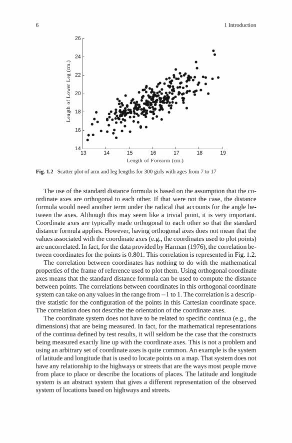
Fig. 1.2 Scatter plot of arm and leg lengths for 300 girls with ages from 7 to 17
The use of the standard distance formula is based on the assumption that the co-ordinate axes are orthogonal to each other. If that were not the case, the distanceformula would need another term under the radical that accounts for the angle be-tween the axes. Although this may seem like a trivial point, it is very important.Coordinate axes are typically made orthogonal to each other so that the standarddistance formula applies. However, having orthogonal axes does not mean that thevalues associated with the coordinate axes (e.g., the coordinates used to plot points)are uncorrelated. In fact, for the data provided by Harman (1976), the correlation be-tween coordinates for the points is 0.801. This correlation is represented in Fig. 1.2.
The correlation between coordinates has nothing to do with the mathematicalproperties of the frame of reference used to plot them. Using orthogonal coordinateaxes means that the standard distance formula can be used to compute the distancebetween points. The correlations between coordinates in this orthogonal coordinatesystem can take on any values in the range from �1 to 1. The correlation is a descrip-tive statistic for the configuration of the points in this Cartesian coordinate space.The correlation does not describe the orientation of the coordinate axes.
The coordinate system does not have to be related to specific continua (e.g., thedimensions) that are being measured. In fact, for the mathematical representationsof the continua defined by test results, it will seldom be the case that the constructsbeing measured exactly line up with the coordinate axes. This is not a problem andusing an arbitrary set of coordinate axes is quite common. An example is the systemof latitude and longitude that is used to locate points on a map. That system does nothave any relationship to the highways or streets that are the ways most people movefrom place to place or describe the locations of places. The latitude and longitudesystem is an abstract system that gives a different representation of the observedsystem of locations based on highways and streets.

1.1 A Conceptual Framework for Thinking About People and Test Items 7
Suppose someone is traveling by automobile between two cities in the UnitedStates, St. Louis and Chicago. The quickest way to do this is to drive along InterstateHighway 55, a direct route between St. Louis and Chicago. It is now standard thatthe distances along highways in the United States are marked with signs called milemarkers every mile to indicate the distance along that highway. In this case, themile markers begin at 1 just across the Mississippi River from St. Louis and end at291 at Chicago. These signs are very useful for specifying exits from the highwayor locating automobiles stopped along the highway. In the context here, the milemarkers can be thought of as analogous to scores on an achievement test that showthe gain in knowledge (the intellectual distance traveled) by a student.
A map of highway Interstate 55 is shown in Fig. 1.3. Note that the highway doesnot follow a cardinal direction and it is not a straight line. Places along the highwaycan be specified by mile markers, but they can also be specified by the coordinatesof latitude and longitude. These are given as ordered pairs of numbers in parenthe-ses. In Fig. 1.3, the two ways of locating a point along the highway are shown for
Fig. 1.3 Locations of citiesalong Interstate Highway55 from East St. Louis toChicago
SpringfieldMile Marker 97(39.85, 89.67)
ChicagoMile Marker 291(41.90, 87.65)

8 1 Introduction
the cities of Springfield, Illinois and Chicago, Illinois, USA. Locations can be spec-ified by a single number, the nearest mile marker, or two numbers, the measures oflatitude and longitude.
It is always possible to locate points using more coordinates than is absolutelynecessary. We could add a third coordinate giving the distance from the center of theEarth along with the latitude and longitude. In the state of Illinois, this coordinatewould have very little variation because the ground is very flat, and it is probablyirrelevant to persons traveling from St. Louis to Chicago. But it does not cause anyharm either. Using too few coordinates can cause problems, however. The coordi-nates of my New York City apartment where I am writing this chapter while onsabbatical are 51st Street, 7th Avenue, and the 14th floor, (51, 7, 14). If only (7,14)is listed when packages are to be delivered, they do not uniquely identify me. It isunlikely that they will ever arrive. Actually, there is even a fourth coordinate (51, 7,14, 21) to identify the specific apartment on the 14th floor. Using too few coordi-nates results in an ambiguous specification of location.
The purpose of this book is to describe methodology for representing the lo-cations of persons in a hypothetical multidimensional cognitive space. As thismethodology is described, it is important to remember that a coordinate systemis needed to specify the locations of persons, but it is not necessary to have theminimum number of coordinates to describe the location, and coordinates do notnecessarily coincide with meaningful psychological dimensions. The coordinatesystem will be defined with orthogonal axes, and the Euclidean distance formulawill be assumed to hold for determining the distance between points. The coordi-nates for a sample of persons may have nonzero correlations, even though the axesare orthogonal.
1.2 General Assumptions Behind Model Development
The methodology described in this book defines mathematical functions that areused to relate the location of a person in a multidimensional Cartesian coordinatespace to the probability of generating a correct response to a test item. This relation-ship is mediated by the characteristics of the test item. The characteristics of the testitem will be represented by a series of values (parameters) that are estimated fromthe item response data. The development of the mathematical function is based ona number of assumptions. These assumptions are similar to those presented in mostitem response theory books, but some additional assumptions have been includedthat are not typically explicitly stated. This is done to make the context of the math-ematical formulation as clear as possible.
The first assumption is that the location of the persons being assessed does notchange during the process of taking the test. This assumption may not be totallytrue in practice – examinees may learn something from interacting with the itemsthat change their locations, or there may be other events that take place in the ex-amination setting (e.g., cheating, information available in the room, etc.) that resultsin some learning. It may be possible to develop models that can capture changes

1.2 General Assumptions Behind Model Development 9
during the process of the test, but that is beyond the scope of the models presentedhere. There are models that consider the changes from one test session to the next(Embretson 1991; Fischer 1995b). These will be placed in the larger context of mul-tidimensional item response theory models.
The second assumption is that the characteristics of a test item remain con-stant over all of the testing situations where it is used. This does not mean thatthe observed statistics used to summarize item performance will remain constant.Certainly, the proportion correct for an item will change depending on the capabil-ities of the sample of examinees. The difficulty of the item has not changed, butthe difficulty has a different representation because of differences in the examineesample. Similarly, a test item written in English may not function very well for stu-dents who only comprehend text written in Spanish. This suggests that one of thecharacteristics of the item is that it is sensitive to differences in language skills ofthe examinee sample, even if that is not the clear focus of the item. This means thatin the full multidimensional representation of the item characteristics, there shouldbe an indicator of the sensitivity to differences in language proficiency. When theexaminee sample does not differ on language proficiency, the sensitivity of test itemto such differences will not be detectable in the test data. However, when variationexists in the examinee population, the sensitivity of the test item to that variationwill affect the probability of correct response to the test item.
A third assumption is that the responses by a person to one test item are inde-pendent of their responses to other test items. This assumption is related to the firstassumption. Test items are not expected to give information that can improve perfor-mance on later items. Similarly, the responses generated by one person are assumedto not influence the responses of another person. One way this could occur is if oneexaminee copies the responses of another. It is expected that the control of the test-ing environment is such that copying or other types of collaboration do not occur.The third assumption is labeled “local independence” in the item response theoryliterature. The concept of local independence will be given a formal definition inChap. 6 when the procedures for estimating parameters are described.
A fourth assumption is that the relationship between locations in the multidi-mensional space and the probabilities of correct response to a test item can berepresented as a continuous mathematical function. This means that for every lo-cation there is one and only one value of probability of correct response associatedwith it and that probabilities are defined for every location in the multidimensionalspace – there are no discontinuities. This assumption is important for the mathemat-ical forms of models that can be considered for representing the interaction betweenpersons and test items.
A final assumption is that the probability of correct response to the test itemincreases, or at least does not decrease, as the locations of examinees increase onany of the coordinate dimensions. This is called the “monotonicity” assumption andit seems reasonable for test items designed for the assessment of cognitive skills andknowledge. Within IRT, there are models that do not require this assumption (e.g.,Roberts et al. 2000). The generalization of such models to the multidimensional caseis beyond the scope of this book.

10 1 Introduction
The next several chapters of this book describe the scientific foundations for themultidimensional item response theory models and several models that are con-sistent with the listed assumptions. These are not the only models that can bedeveloped, but also they are models that are currently in use. There is some empiri-cal evidence that these models provide reasonable representations of the relationshipbetween the probability of correct response to a test item and the location of a per-son in a multidimensional space. If that relationship is a reasonable approximationto reality, practical use can be made of the mathematical models. Such applicationswill be provided in the latter chapters of the book.
1.3 Exercises
1. Carefully read the following test item and select the correct answer. Develop alist of all of the skills and knowledge that you believe are needed to have a highprobability of selecting the correct answer.
The steps listed below provide a recipe for converting temperature measured indegrees Fahrenheit .F / into the equivalent in degrees Celsius (C).
1. Subtract 32 from a temperature given in degrees Fahrenheit.2. Multiply the resulting difference by 5.3. Divide the resulting product by 9.
Which formula is a correct representation of the above procedure?
A. C D F � 32 � 5=9B. C D .F � 32/ � 5=9C. C D F � .32 � 5/=9D. C D F � 32 � .5=9/E. C D F � .32 � 5=9/
2. In our complex society, it is common to identify individuals in a number of differ-ent ways. Sometimes it requires multiple pieces of information to uniquely identifya person. For example, it is possible to uniquely identify students in our graduateprogram from the following information: year of entry, gender (0,1), advisor, officenumber – (2004, 1, 3, 461). Think of ways that you can be uniquely identified fromstrings of numbers and other ways you can be identified with one number.
3. Which of the following mathematical expressions is an example of a function ofx and which is not? Give the reasons for your classification.
A. y D x3 � 2x2 C 1
B. y2 D x
C. z2 D x2 C y2
Chapter 2Unidimensional Item Response Theory Models
In Chap. 3, the point will be made that multidimensional item response theory(MIRT) is an outgrowth of both factor analysis and unidimensional item responsetheory (UIRT). Although this is clearly true, the way that MIRT analysis resultsare interpreted is much more akin to UIRT. This chapter provides a brief introduc-tion to UIRT with a special emphasis on the components that will be generalizedwhen MIRT models are presented in Chap. 4. This chapter is not a thorough des-cription of UIRT models and their applications. Other texts such as Lord (1980),Hambleton and Swaminathan (1985), Hulin et al. (1983), Fischer and Molenaar(1995), and van der Linden and Hambleton (1997) should be consulted for a morethorough development of UIRT models.
There are two purposes for describing UIRT models in this chapter. The first isto present basic concepts about the modeling of the interaction between persons andtest items using simple models that allow a simpler explication of the concepts. Thesecond purpose is to identify shortcomings of the UIRT models that motivated thedevelopment of more complex models. As with all scientific models of observedphenomena, the models are only useful to the extent that they provide reasonableapproximations to real world relationships. Furthermore, the use of more complexmodels is only justified when they provide increased accuracy or new insights. Oneof the purposes of this book is to show that the use of the more complex MIRTmodels is justified because they meet these criteria.
2.1 Unidimensional Models of the Interactions of Personsand Test Items
UIRT comprises a set of models (i.e., item response theories) that have as a ba-sic premise that the interactions of a person with test items can be adequatelyrepresented by a mathematical expression containing a single parameter describ-ing the characteristics of the person. The basic representation of a UIRT model isgiven in (2.1). In this equation, � represents the single parameter that describes thecharacteristics of the person, � represents a vector of parameters that describe thecharacteristics of the test item, U represents the score on the test item, and u is
M.D. Reckase, Multidimensional Item Response Theory, Statistics for Socialand Behavioral Sciences, DOI 10.1007/978-0-387-89976-3 2,c� Springer Science+Business Media, LLC 2009
11

12 2 Unidimensional Item Response Theory Models
a possible value for the score, and f is a function that describes the relationshipbetween the parameters and the probability of the response, P(U D u).
P.U D u j �/ D f .�;�; u/: (2.1)
The item score, u, appears on both sides of the equation because it is often usedin the function to change the form of the function depending on the value of thescore. This is done for mathematical convenience. Specific examples of this use willbe provided later in this chapter.
The assumption of a single person parameter for an IRT model is a strongassumption. A substantial amount of research has been devoted to determiningwhether this assumption is reasonable when modeling a particular set of item re-sponse data. One type of research focuses on determining whether or not the datacan be well modeled using a UIRT model. For example, the DIMTEST proceduredeveloped by Stout et al. (1999) has the purpose of statistically testing the assump-tion that the data can be modeled using a function like the one given in (2.1) with asingle person parameter. Other procedures are available as well (see Tate 2003 for asummary of these procedures). The second type of research seeks to determine theeffect of ignoring the complexities of the data when applying a UIRT model. Theseare generally robustness studies. Reckase (1979) presented one of the first studiesof this type, but there have been many others since that time (e.g., Drasgow andParsons 1983; Miller and Linn 1988; Yen 1984).
Along with the assumption of a single person parameter, � , most UIRT modelsassume that the probability of selecting or producing the correct response to a testitem scored as either correct or incorrect increases as � increases. This assumption isusually called the monotonicity assumption. In addition, examinees are assumed torespond to each test item as an independent event. That is, the response by a personto one item does not influence the response to an item produced by another person.Also, the response by a person to one item does not affect that person’s tendenciesto respond in a particular way to another item. The response of any person to anytest item is assumed to depend solely on the person’s single parameter, � , and theitem’s vector of parameters, �. The practical implications of these assumptions arethat examinees do not share information during the process of responding to the testitems, and information from one test item does not help or hinder the chances ofcorrectly responding to another test item. Collectively, the assumption of indepen-dent responses to all test items by all examinees is called the local independenceassumption.
The term “local” in the local independence assumption is used to indicate thatresponses are assumed independent at the level of individual persons with the samevalue of � , but the assumption does not generalize to the case of variation in � .For groups of individuals with variation in the trait being assessed, responses todifferent test items typically are correlated because they are all related to levels ofthe individuals’ traits. If the assumptions of the UIRT model hold, the correlationbetween item scores will be solely due to variation in the single person parameter.
2.1 Unidimensional Models of the Interactions of Persons and Test Items 13
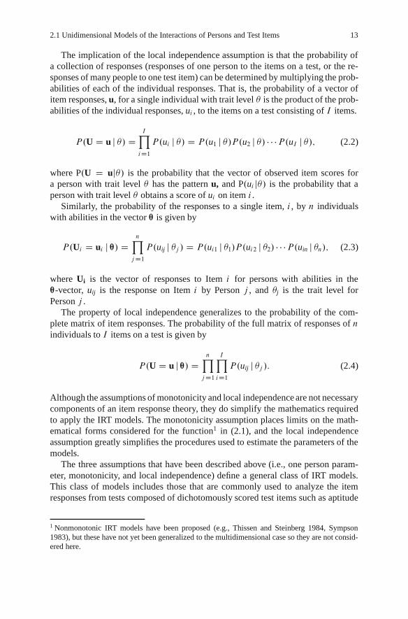
The implication of the local independence assumption is that the probability ofa collection of responses (responses of one person to the items on a test, or the re-sponses of many people to one test item) can be determined by multiplying the prob-abilities of each of the individual responses. That is, the probability of a vector ofitem responses, u, for a single individual with trait level � is the product of the prob-abilities of the individual responses, ui , to the items on a test consisting of I items.
P.U D u j �/ DIY
iD1P.ui j �/ D P.u1 j �/P.u2 j �/ � � �P.uI j �/; (2.2)
where P.U D uj�/ is the probability that the vector of observed item scores fora person with trait level � has the pattern u, and P.ui j�/ is the probability that aperson with trait level � obtains a score of ui on item i .
Similarly, the probability of the responses to a single item, i , by n individualswith abilities in the vector ™ is given by
P.Ui D ui j ™/ DnY
jD1P.uij j �j / D P.ui1 j �1/P.ui2 j �2/ � � �P.uin j �n/; (2.3)
where Ui is the vector of responses to Item i for persons with abilities in the™-vector, uij is the response on Item i by Person j , and �j is the trait level forPerson j .
The property of local independence generalizes to the probability of the com-plete matrix of item responses. The probability of the full matrix of responses of nindividuals to I items on a test is given by
P.U D u j ™/ DnY
jD1
IY
iD1P.uij j �j /: (2.4)
Although the assumptions of monotonicity and local independence are not necessarycomponents of an item response theory, they do simplify the mathematics requiredto apply the IRT models. The monotonicity assumption places limits on the math-ematical forms considered for the function1 in (2.1), and the local independenceassumption greatly simplifies the procedures used to estimate the parameters of themodels.
The three assumptions that have been described above (i.e., one person param-eter, monotonicity, and local independence) define a general class of IRT models.This class of models includes those that are commonly used to analyze the itemresponses from tests composed of dichotomously scored test items such as aptitude
1 Nonmonotonic IRT models have been proposed (e.g., Thissen and Steinberg 1984, Sympson1983), but these have not yet been generalized to the multidimensional case so they are not consid-ered here.

14 2 Unidimensional Item Response Theory Models
and achievement tests. This class of models can be considered as a general psycho-metric theory that can be accepted or rejected using model checking procedures.The assumption of local independence can be tested for models with a single personparameter using the procedures suggested by Stout (1987) and Rosenbaum (1984).These procedures test whether the responses to items are independent when a sur-rogate for the person parameter, such as the number-correct score, is held constant.If local independence conditional on a single person parameter is not supported byobserved data, then item response theories based on a single person parameter arerejected and more complex models for the data should be considered.
The general form of IRT model given in (2.1) does not include any specificationof scales of measurement for the person and item parameters. Only one scale has de-fined characteristics. That scale is for the probability of the response to the test itemthat must range from 0 to 1. The specification of the function, f , must also includea specification for the scales of the person parameter, � , and the item parameters, �.The relative size and spacing of units along the �-scale are determined by the se-lection of the form of the mathematical function used to describe the interactionof persons and items. That mathematical form sets the metric for the scale, but thezero point (origin) and the units of measurement may still not be defined. Lineartransformations of a scale retain the same shape for the mathematical function.
For an IRT model to be considered useful, the mathematical form for the modelmust result in reasonable predictions of probabilities of all item scores for all per-sons and items in a sample of interest. The IRT model must accurately reflect theseprobabilities for all items and persons simultaneously. Any functional form for theIRT model will fit item response data perfectly for a one-item test because the lo-cations of the persons on the �-scale are determined by their responses to the oneitem. For example, placing all persons with a correct response above a point on the�-scale and all of those with an incorrect response below that point and specifying amonotonically increasing mathematical function for the IRT model will insure thatpredicted probabilities are consistent with the responses. The challenge to develop-ers of IRT models is to find functional forms for the interaction of persons and itemsthat apply simultaneously to the set of responses by a number of persons to all ofthe items on a test.
The next section of this chapter summarizes the characteristics of several IRTmodels that have been shown to be useful for modeling real test data. The modelswere chosen for inclusion because they have been generalized to the multidimen-sional case. No attempt is made to present a full catalogue of UIRT models. Thefocus is on presenting information about UIRT models that will facilitate the under-standing of their multidimensional generalizations.
2.1.1 Models for Items with Two Score Categories
UIRT models that are most frequently applied are those for test items that are scoredeither correct or incorrect – usually coded as 1 and 0, respectively. A correct re-sponse is assumed to indicate a higher level of proficiency than an incorrect response

2.1 Unidimensional Models of the Interactions of Persons and Test Items 15
so monotonically increasing mathematical functions are appropriate for modelingthe interactions between persons and items. Several models are described in thissection, beginning with the simplest. Models for items with two score categories(dichotomous models) are often labeled according to the number of parameters usedto summarize the characteristics of the test items. That convention is used here.
2.1.1.1 One-Parameter Logistic Model
The simplest commonly used UIRT model has one parameter for describing thecharacteristics of the person and one parameter for describing the characteristics ofthe item. Generalizing the notation used in (2.1), this model can be represented by
P.Uij D uij j �j / D f .�j ; bi ; uij/; (2.5)
where uij is the score for Person j on Item i (0 or 1), �j is the parameter that de-scribes the relevant characteristics of the j th person – usually considered to be anability or achievement level related to performance on Item i , and bi is the param-eter describing the relative characteristics of Item i – usually considered to be ameasure of item difficulty.2
Specifying the function in (2.5) is the equivalent of hypothesizing a unique,testable item response theory. For most dichotomously scored cognitive test items, afunction is needed that relates the parameters to the probability of correct responsein such a way that the monotonicity assumption is met. That is, as �j increases, thefunctional form of the model should specify that the probability of correct responseincreases. Rasch (1960) proposed the simplest model that he could think of that metthe required assumptions. The model is presented below:
P.uij D 1 jAj ;Bi / D AjBi
1C AjBi; (2.6)
where Aj is the single person parameter now generally labeled �j, and Bi is thesingle item parameter now generally labeled bi .
This model has the desired monotonicity property and the advantage of simplic-ity. For the function to yield values that are on the 0 to 1 probability metric, theproduct of AjBi can not be negative because negative probabilities are not defined.To limit the result to the required range of probabilities, the parameters are definedon the range from 0 to 1.
The scale for the parameters for the model in (2.6) makes some intuitive sense.A 0 person parameter indicates that the person has a 0 probability of correct responsefor any item. A 0 item parameter indicates that the item is so difficult that no matter
2 The symbols used for the presentation of the models follow Lord (1980) with item parametersrepresented by Roman letters. Other authors have used the statistical convention of representingparameters using Greek letters.

16 2 Unidimensional Item Response Theory Models
how high the ability of the persons, they still have a 0 probability of correct re-sponse. In a sense, this model yields a proficiency scale that has a true 0 point and itallows statements like “Person j has twice the proficiency of Person k.” That is, thescales for the model parameters have the characteristics of a ratio scale as definedby Stevens (1951).
Although it would seem that having a model with ratio scale properties would bea great advantage, there are also some disadvantages to using these scales. Supposethat the item parameter Bi D 1. Then a person with parameter Aj D 1 will have a.5 probability of correctly responding to the item. All persons with less then a .5probability of correctly responding to the test item will have proficiency estimatesthat are squeezed into the range from 0 to 1 on the A-parameter scale. All personswith greater than a .5 probability of correct response will be stretched over the rangefrom 1 to 1 on the proficiency scale. If test items are selected for a test so that abouthalf of the persons respond correctly, the expected proficiency distribution is veryskewed. Figure 2.1 provides an example of such a distribution.
The model presented in (2.6) is seldom seen in current psychometric literature.Instead, a model based on a logarithmic transformation of the scales of the parame-ters (Fischer 1995a) is used. The equation for the transformed model is
P.uij D 1 j �j ; bi / D e�j�bi1C e�j�bi D �.�j � bi/; (2.7)
where � is the cumulative logistic density function, e is the base of the naturallogarithms, and �j and bi are the person and item parameters, respectively.
0 5 10 15 20 250
50
100
150
200
250
300
350
A-Parameter Scale
Freq
uenc
y
Fig. 2.1 Possible distribution of person parameters for the model in (2.6)

2.1 Unidimensional Models of the Interactions of Persons and Test Items 17
Because this model uses the logistic density function and because it has onlya single item parameter, it is often called the one-parameter logistic IRT model.Alternatively, because it was originally suggested by Rasch (1960, 1961), it is calledthe Rasch model. The relationship between the models in (2.7) and (2.6) can eas-ily be determined by substituting the transformations of the parameters into (2.7):�j D ln.Aj/ and bi D � ln.Bi /.
The scale of the person parameter in (2.7) ranges from �1 to 1 rather thanfrom 0 to 1 for the model in (2.6). The scale for the item parameter is the same forthat of the person parameter, but the direction of the scales are reversed from (2.6)to (2.7). Large values of the Bi parameter indicate easy items while small valuesof bi indicate easy items. Thus, the bi parameter is legitimately called a difficultyparameter while Bi is an “easiness” parameter.
The models in (2.6) and (2.7) show the flexibility that exists when hypothesiz-ing IRT models. These two models will fit real test data equally well because themodel parameters are a monotonic transformation of each other. Yet, the scales forthe parameters are quite different in character. Equation (2.6) uses scales with a log-ical zero point while the parameters in (2.7) do not have that characteristic. It isdifficult to say which model is a correct representation of the interactions betweenpersons and an item. Generally, (2.7) seems to be preferred because estimation ismore convenient and it has a clear relationship to more complex models.
Some researchers state that the Rasch model provides an interval scale of mea-surement using the typology defined by Stevens (1946). All IRT models have aninterval scale for the person parameter as an unstated assumption because the formof the equation is not defined unless the scale of the person parameter has inter-val properties. But, in (2.6) and (2.7) we have two interval scales that are nonlineartransformations of each other. This would contradict the permissible transformationsallowed by Stevens (1946). The point is that these scales are arbitrary decisions ofthe model builder. The usefulness of the scales comes from the ease of interpretationand the relationships with other variables, not inherent theoretical properties.
The form of (2.7) is shown graphically in Fig. 2.2. The graph shows the relation-ship between � and the probability a person at that trait level will provide a correctresponse for an item with b-parameter equal to .5. The graph clearly shows themonotonically increasing relationship between trait level and probability of correctresponse from the model. It also shows that this model has a lower asymptote forthe probability of 0 and an upper asymptote of 1. The graph of the probability of acorrect response as a function of � is typically called an item characteristic curveor ICC.
Several characteristics of this model can be derived through some relatively sim-ple analysis. A cursory look at the graph in Fig. 2.2 shows that the curve is steeper(i.e., has greater slope) for some values of � then for others. When the slope is fairlysteep, the probability of correct response to the item is quite different for individ-uals with �-values that are relatively close to each other. In regions where the ICCis fairly flat – has low slope – the �-values must be relatively far apart before theprobability of correct response results in noticeable change.

18 2 Unidimensional Item Response Theory Models
–4 –3 –2 –1 0 1 2 3 40
0.1
0.2
0.3
0.4
0.5
0.6
0.7
0.8
0.9
1
θ
Prob
abili
ty
Fig. 2.2 One-parameter logistic model item characteristic curve for b D :5
For example, a person with � D :25 has a probability of correct response to thetest item of .44 if the model is correct. A person .5 units higher on the �-scale (i.e.,� D :75) has a probability of correct response of .56 if the model is correct. Thedifference in these two probabilities for the .5-unit change on � is .12. At � D �1:5,the probability of correct response is .12. At � D � 1:0, a .5 unit change from theoriginal value, the probability of correct response is .18. Over this .5 unit change inthe �-scale, the change in probability is only .06. This analysis indicates that thetest item described by the ICC in Fig. 2.2 would be better at differentiating betweenpersons between .25 and .75 on the �-scale than persons between �-values of �1:5and �1:0.
A more analytic way of considering this issue is to determine the slope of theICC at each point on the �-scale so that the steepness of the ICC can be determinedfor any value of � . The first derivative of the function describing the interaction ofthe persons and the item provides the slope of the ICC at each value of � . For themodel given in (2.7), the first derivative of P.uij D 1 j �j; bi / with respect to � isgiven by the following expression:
@P
@�D P � P2 D P.1 � P/ D PQ; (2.8)
where, for simplicity,P D P.uij D 1 j �j; bi /;
andQD .1 � P/.From this expression, it is clear that the slope of the ICC is 0 (i.e., the curve is
horizontal) only when the probability of correct response is 0 or 1. This confirms

2.1 Unidimensional Models of the Interactions of Persons and Test Items 19
that the asymptotes for the model are 0 and 1. Note that the slope of the ICC is equalto .25 (that is, 1=4, a point that will be important later) when the probability of correctresponse is .5. A probability of .5 is the result of the model when �j is equal to bi in(2.7) because then the exponent is equal to 0 and e0 =1 yielding a probability of 1=2.
Note that the difference in probability of correct response for � values of .25 and.75 (centered around � D :5) was .12. The slope at � D :5 can be approximated asthe ratio of the difference in probability (.12) over the range of �s to the difference in� values .:5/ � :12=:5D :24. Because this ratio gives the slope for a linear functionand the ICC is nearly linear in the �-range from .25 to .75, it is not surprising that theslope from (2.8) and the approximation have nearly the same value. The similaritymerely confirms that the derivative with respect to � provides the slope.
To determine where along the �-scale, the test item is best at differentiating peo-ple who are close together on the scale, the derivative of the expression for the slope,(2.8), can be used. This is the second derivative of (2.7) with respect to � . Settingthe second derivative to 0 and solving for � yields the point on the �-scale wherethe test item is most discriminating – the point of maximum slope. The derivative of(2.8) with respect to � is
@.P � P2/
@�D .P � P2/.1� 2P /: (2.9)
Solving this expression for 0 yields values of P of 0, 1, and .5. The values of� that correspond to the values of 0 and 1 are �1 and 1, respectively. The onlyfinite solution for a value of � corresponds to the value of P D :5. That is, the slopeof the function is steepest when � has a value that results in a probability of correctresponse from the model of .5. As previously noted, a .5 probability results when� is equal to bi . Thus, the b-parameter indicates the point on the �-scale where theitem is most discriminating. Items with high b-parameters are most discriminatingfor individuals with high trait levels – those with high �-values. Items with lowb-parameters are most discriminating for individuals with low trait levels.
The b-parameter also provides information about the ranges of trait levels forpersons that are likely to respond correctly or incorrectly to the test item. Those per-sons with �-values greater than bi have a greater than .5 probability of respondingcorrectly to Item i . Those with �-values below bi have less than a .5 probability ofresponding correctly to the item. This interpretation of the b-parameter is depen-dent on the assumption that the model in (2.7) is an accurate representation of theinteraction of the persons and the test item.
Because the b-parameter for the model provides information about the trait levelthat is best measured by the item and about the likely probability of correct response,it has been labeled the difficulty parameter for the item. Although this terminologyis somewhat of an oversimplification of the complex information provided by thisparameter, the label has been widely embraced by the psychometric community.
It is important to note that for the model given in (2.7), the value of the maximumslope is the same for all items. The only feature of the ICC that changes from testitem to test item is the location of the curve on the �-scale. Figure 2.3 shows ICCs

20 2 Unidimensional Item Response Theory Models
–4 –3 –2 –1 0 1 2 3 40
0.1
0.2
0.3
0.4
0.5
0.6
0.7
0.8
0.9
1
θ
Prob
abili
ty
Fig. 2.3 ICCs for the model in (2.7) for bi D �1, .25, 1.75
for three different items. The items have b-parameters with values of 1.75, .25,and �1:0. The graphs in Fig. 2.3 show that the slopes of the three curves are thesame where they cross the P D :5 line. Because the ICCs for the model have acommon value for the maximum slope for the items, the model is said to include anassumption that all test items have the same discriminating power. This is not truein an absolute sense because at different values of � the slopes of the various itemsdiffer. But it is true that a set of items that are consistent with this model will havethe same maximum slope, and the magnitude of the maximum slope at P D :5 willbe 1=4 for all items.
The one-parameter logistic (Rasch) model has a number of advantages over morecomplex models including simplicity in form and mathematical properties that makethe estimation of the parameters of the model particularly convenient. One con-venient mathematical property is that there is a direct relationship between thenumber-correct scores for a set of test items and the estimates of � . All persons withthe same number-correct score have the same maximum-likelihood estimate of � .3
A similar relationship exists between the number of correct responses to a test itemand the maximum-likelihood estimate of the b-parameter for the test item. All itemswith the same proportion of correct responses for a sample of examinees have thesame maximum-likelihood b-parameter estimate based on that sample. These rela-tionships allow the �-parameters for the examinees to be estimated independentlyof the b-parameters for the test items. A significant contingent of the psychometric
3 Chapter 6 presents a number of estimation procedures including maximum likelihood. A fulldiscussion of estimation procedures is beyond the scope of this book. The reader should referto a comprehensive mathematical statistics text for a detailed discussion of maximum-likelihoodestimation and other techniques for estimating model parameters.

2.1 Unidimensional Models of the Interactions of Persons and Test Items 21
community maintains that these properties of the one-parameter (Rasch) model areso desirable that models that do not have these properties should not be considered.The perspective of this group is that only when person and item-parameters can beestimated independently of each other do �-estimates result in numbers that canbe called measurements. Andrich (2004) provides a very clear discussion of thisperspective and contrasts it with alternative views.
The perspective taken here is that the goal of the use of IRT models is to describethe interaction between each examinee and test item as accurately as possible withinthe limitations of the data and computer resources available for test analysis. Thisperspective is counter to the one that proposes that strict mathematical criteria areneeded to define measurement and only models that meet the criteria are accept-able. Rather, the value of a model is based on the accuracy of the representationof the interaction between persons and items. The estimates of parameters of suchmodels are used to describe the characteristics of the persons and items. The strictrequirements for independent estimation of person and item parameters will not beconsidered as a requirement for a useful psychometric model.
From this perspective, whether or not the one-parameter logistic model is ad-equate for describing the interaction of examinees with test items is an empiricalquestion rather than a theoretical question. For example, when test forms areanalyzed using traditional item analysis procedures, the usual result is that the point-biserial and biserial correlation indices of the discriminating power of test items varyacross items. Lord (1980) provides an example of the variation in discrimination in-dices for data from a standardized test. Item analysis results of this kind providestrong evidence that test items are not equal in discriminating power. These resultsimply that a model that has the same value for the maximum slope of the ICCs for alltest items does not realistically describe the interaction between persons and items.
2.1.1.2 Two-Parameter Logistic Model
Birnbaum (1968) proposed a slightly more complex model than the one presentedin (2.7). The mathematical expression for the model is given by
P.Uij D 1 j �j ; ai ; bi / D eai .�j�bi /
1C eai .�j�bi / ; (2.10)
where ai is a parameter related to the maximum slope of the ICC and the othersymbols have the same definition as were given for (2.7). The first partial derivativeof this model with respect to �j, which gives the slope of the ICC at each value of�j, is given by
@P.Uij D 1 j �j ; ai ; bi /@�j
D aiP2Q2 D ai .P2 � P22 /; (2.11)

22 2 Unidimensional Item Response Theory Models
where P2 is the probability of a correct response for the model given in (2.10), andQ2 D .1 � P2/. The subscript “2” is used to distinguish the probability estimatesfrom the model in (2.10) from those for the model in (2.7).
The partial derivative of the slope with respect to �j, which is the same as thesecond partial derivative of the model in (2.10) with respect to �j, is given by
@.aiP2Q2/
@�jD a2i .P2 � P2
2 /.1 � 2P2/: (2.12)
Solving this expression for zero to determine the point of maximum slope shows thatthe only finite solution occurs when P2 D :5, as was the case for the one-parameterlogistic model. Substituting .5 into (2.11) gives the value of the maximum slope,ai /4. This result shows that the ai parameter controls the maximum slope of theICC for this model. It should also be noted that the point of maximum slope occurswhen �j D bi , just as was the case for the one-parameter logistic model. Thus, biin this model can be interpreted in the same way as for the one-parameter logisticmodel – as the difficulty parameter.
Figure 2.4 presents three examples of ICCs with varying a- and b-parameters.These ICCs are not parallel at the point where they cross the .5 probability line.Unlike the ICCs for the one-parameter logistic model, these curves cross each other.This crossing of the curves allows one test item to be harder than another test itemfor persons at one point on the �-scale, but easier than that same item for personsat another point on the �-scale. For example at � D � 1, Item 1 is easier thanItem 2 (the probability of correct response is greater), but at � D 1, Item 1 is more
–4 –3 –2 –1 0 1 2 3 40
0.1
0.2
0.3
0.4
0.5
0.6
0.7
0.8
0.9
1
θ
Prob
abili
ty
Item 1Item 2Item 3
Fig. 2.4 Item characteristic curves for the two-parameter logistic model with a-parameters .7, 1.4,.56 and b-parameters .5, 0, �1:2, respectively
2.1 Unidimensional Models of the Interactions of Persons and Test Items 23
difficult than Item 2 (its probability of correct response is lower). This result is adirect consequence of the difference in the discriminating power (i.e., difference ina-parameters) of the items.
The a-parameter for the two-parameter logistic model also enters into the esti-mation of the �-parameter for each examinee. While for the one-parameter logisticmodel, all examinees with the same number-correct score have the same estimateof � , for the two-parameter logistic model, the examinees with the same weighted
score, Sj given by Sj DIP
iD1aiuij, have the same maximum likelihood estimate of � .
Use of the two-parameter logistic model has the effect of weighting highly discrim-inating items – those with steeper maximum slopes – more heavily when estimating� than items that are less discriminating. While for the one-parameter logistic modelit does not matter which items the examinee answers correctly, the estimate of � isdependent only on the number of correct responses, for the two-parameter logisticmodel, the particular test items responded to correctly affect the estimate of � . Bakerand Kim (2004) provide a thorough discussion of person parameter estimation forthe different models.
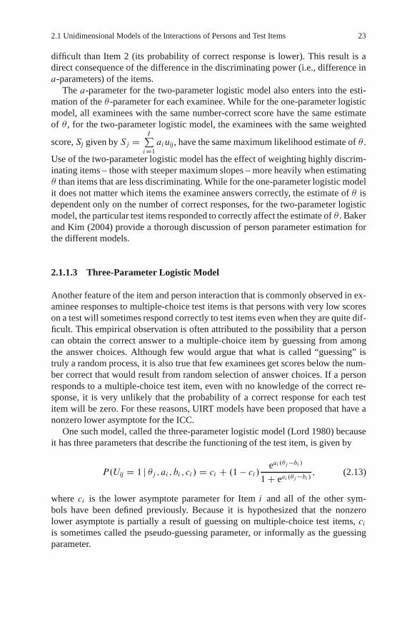
2.1.1.3 Three-Parameter Logistic Model
Another feature of the item and person interaction that is commonly observed in ex-aminee responses to multiple-choice test items is that persons with very low scoreson a test will sometimes respond correctly to test items even when they are quite dif-ficult. This empirical observation is often attributed to the possibility that a personcan obtain the correct answer to a multiple-choice item by guessing from amongthe answer choices. Although few would argue that what is called “guessing” istruly a random process, it is also true that few examinees get scores below the num-ber correct that would result from random selection of answer choices. If a personresponds to a multiple-choice test item, even with no knowledge of the correct re-sponse, it is very unlikely that the probability of a correct response for each testitem will be zero. For these reasons, UIRT models have been proposed that have anonzero lower asymptote for the ICC.
One such model, called the three-parameter logistic model (Lord 1980) becauseit has three parameters that describe the functioning of the test item, is given by
P.Uij D 1 j �j ; ai ; bi ; ci / D ci C .1 � ci /eai .�j�bi /
1C eai .�j�bi / ; (2.13)
where ci is the lower asymptote parameter for Item i and all of the other sym-bols have been defined previously. Because it is hypothesized that the nonzerolower asymptote is partially a result of guessing on multiple-choice test items, ciis sometimes called the pseudo-guessing parameter, or informally as the guessingparameter.

24 2 Unidimensional Item Response Theory Models
The influence of the ci -parameter on the ICC can be determined by a straight-forward application of limits. As � approaches negative infinity, the probabilityof correct response to a test item that is accurately described by this model ap-proaches ci .
lim�! �1
�ci C .1 � ci / eai .�j�bi /
1C eai .�j�bi /
�D ci C .1 � ci / lim
�! �1
�eai .�j�bi /
1C eai .�j�bi /
�
D ci C .1 � ci / 0 D ci : (2.14)
The relationship between the lower asymptote of the ICC and the value of cican clearly be seen in the ICC for the model in (2.13) with ai D 1:8, bi D 1:5, andci D :16. The plot of the ICC is given in Fig. 2.5. In the plot, the probability of .16 isindicated by the dashed line. It is clear that no matter how low the trait level of theexaminee, the probability of correct response to the test item from the model doesnot fall below .16.
The slope of the ICC at points along the �-scale can be determined in thesame way as for the previous models. The partial derivative of (2.13) with respectto � gives the slope at each point. To simplify the expression for the slope andmaximum slope, P3 is used to refer to the left side of (2.13). The right side is repre-sented by ci C .1� ci /P2, where P2 is the expression for the two-parameter logisticmodel given in (2.10). This notation not only clarifies the mathematics involvedin determining the slope and maximum slope of the ICC, but also emphasizes therelationship between the two and three-parameter logistic models.
–4 –3 –2 –1 0 1 2 3 40.1
0.2
0.3
0.4
0.5
0.6
0.7
0.8
0.9
1
θ
Prob
abili
ty
Fig. 2.5 ICC for an item described by the three-parameter logistic model

2.1 Unidimensional Models of the Interactions of Persons and Test Items 25
Given the above substitutions in (2.13), the slope of the three-parameter logisticmodel is given by
@P3
@�D .1� ci /aiP2Q2 D .1� ci /aiP2.1�P2/ D .1� ci /ai .P2 �P2
2 /: (2.15)
From this result, it is clear that the slope is a function of all of the item param-eters in the model. The point of maximum slope can be determined by taking thederivative of the slope with respect to � , setting the resulting expression equal tozero and solving the equation for � . Note that the derivative of the slope is also thesecond derivative of the model with respect to � , and therefore it also identifies thepoint of inflection of the ICC. The maximum slope is given by the solution of
@�.1 � ci /ai .P2 � P2
2 /�
@�D .1 � ci /a
2i .P2 � P2
2 /.1 � 2P2/ D 0: (2.16)
The maximum slope is achieved whenP2 (notP3) is .5. WhenP2 D :5, P3 D ciC.1�ci /�:5. This value is half way between ci and 1. The point of maximum slope oc-curs where the ICC crosses the line P3 D .ci C 1/=2. In Fig. 2.5, this value is shownas the broken line for P3 D :58. Referring back to (2.10), P2 D :5 when �j D bi .Thus, the b-parameter still indicates the point on the �-scale where the ICC hasmaximum slope.
SubstitutingP2 D :5 into (2.15) gives the maximum value of the slope. In general,that value is given by (1� ci /ai=4. When a nonzero lower asymptote is added to themodel, the slope of the ICC at its maximum is less than that for the two-parameterlogistic model with the same ai and bi parameters.
2.1.1.4 Other UIRT Models
The three models described so far were selected to show the effect of adding itemparameters to IRT models and the function and meaning of the item parametersthat are most commonly encountered. Although these three models are among themost commonly used of the UIRT models, many other alternative models exist, andeven more can be imagined. Any mathematical function that maps a single vari-able describing examinee capabilities into numbers that range from 0 to 1 can beused as an UIRT model. Linear functions (Lazarsfeld 1966), polynomial functions(McDonald 1967; Samejima and Livingston 1979; Sympson 1983), spline func-tions (Abrahamowicz and Ramsay 1992), and normal ogive functions (Lord andNovick 1968) have been used. While a full discussion of these different modelswould unnecessarily distract from the goals of this chapter, UIRT models based onthe normal ogive function are presented because of their importance to the develop-ment of MIRT models.

26 2 Unidimensional Item Response Theory Models
The normal ogive equivalent to the three-parameter logistic model is given by
P.Uij D 1 j �j ; ai ; bi ; ci / D ci C .1 � ci /zZ
�1
1p2�
e� z22 dz; (2.17)
where z D ai .�j � bi/ and all of the person and item parameters have the samedefinitions as for the logistic models. The integral specified in the model defines thearea under the standard normal distribution from negative infinity to z.
The normal ogive model has slightly steeper ICCs than the logistic model forthe same set of item parameter values. To compensate for this difference, Birnbaum(1968) suggested multiplying the exponents in the logistic model by 1.7 to make thetwo models more similar. When the 1.7 is included in the model, the predicted prob-abilities differ by less than .01 for all values of � . That is, if the logistic componentof the two and three-parameter logistic models is changed to
e1:7ai .�j�bi /
1C e1:7ai .�j�bi / ; (2.18)
then the ICCs for the logistic and normal ogive models with the same item param-eters will be virtually identical. The constant, 1.7, is sometimes represented by thesymbolD in the exponents of the logistic models.
2.1.2 Relationships Between UIRT Parameters and ClassicalItem Statistics
In the discussion of UIRT models for items with two score categories, three param-eters (a, b, and c) have been defined. These parameters determine the form of theICCs for the test items. These parameters have been given descriptive labels (e.g.,difficulty) that have certain intuitive meanings. These same descriptive labels oftenhave definitions in the context of classical test theory. This section provides informa-tion about the connections between the IRT-based item parameters and the classicaltest theory item statistics that use similar terms as labels.
2.1.2.1 Item Difficulty
In classical test theory, item difficulty refers to the proportion of a sample of exami-nees that give a correct response to a test item. Because the number is a proportion,it ranges from 0 to 1 with numbers near 1 indicating easy test items and those near0 indicating difficult test items. Because test items are easier as the index increases,some have argued that it is really a descriptor of the easiness of test items rather than

2.1 Unidimensional Models of the Interactions of Persons and Test Items 27
their difficulty. However, the term “difficulty” continues in common usage for thisstatistic. The statistic is often referred to as a p-value, an abbreviation for proportioncorrect.
The b-parameter that appears in many IRT models indicates the point on the traitscale where the ICC has the steepest slope. For models without a lower asymptoteparameter, this occurs at the trait level where the examinee has a .5 probability ofgetting the item correct. Changing the b-parameter in the model shifts the ICC to theright or left without affecting the shape of the curve. As the b-parameter increases,the curve shifts to the right (toward higher �-values) and the probability of correctresponse to the test item at a particular �-value is lower. Therefore, higher b-valuesindicate more difficult test items. Lower b-values indicate easier items. Becausedifficulty increases with increased b-value, it is reasonable to label b-parametersdifficulty parameters.
To determine the p-value that corresponds to a b-value, the distribution of �for a group of examinees must be known. This fact emphasizes the sample specificnature of the classical item difficulty index (p-value) as a measure of the difficultyof the test item. If the distribution of � is given by f .�/, the relationship betweenthe p-value and the b-parameter is given by
pi D1Z
�1P.ui D 1 j �i ; bi /f .�/d�; (2.19)
where pi is the proportion of examinees in the sample that answer the item correctly(the classical item difficulty for Item i ), and �i is the vector of other item parametersfor Item i that may be included in the model (e.g., ai , and ci ). The other symbolswere defined previously.
Equation (2.19) provides some insights into the relationship between p and b.If all of the other item parameters in the IRT model are held constant, and theb-parameter is increased in magnitude, the probability of correct response at all�-values becomes smaller. Accordingly, all values of the product of the probabil-ity of correct response and the density of � will become smaller. Consequently, thevalue of the integral will be smaller and the p-value will be smaller. This impliesthat if the values of the other item parameters are held constant, the p-values arefunctionally related to the b-parameters for a specific sample of examinees. Be-cause the one-parameter logistic model does not have any other item parameters,this functional relationship is always present. The relationship is not a linear onebecause the p-values are restricted to the range from 0 to 1 while the b-parametershave an infinite range of possible values. Note also that the relationship is an inverseone. As the b-values increase, the p-values decrease. The plot in Fig. 2.6 shows therelationship between the b-parameters for the one-parameter logistic model and thep-values for a sample of 200 examinees sampled from a standard normal distribu-tion. The slight variation in the points from a curve is due to sampling variation inthe p-values.

28 2 Unidimensional Item Response Theory Models
–4 –3 –2 –1 0 1 2 3 40
0.1
0.2
0.3
0.4
0.5
0.6
0.7
0.8
0.9
1
b-parameter
p-va
lue
Fig. 2.6 Relationship between the one-parameter logistic model b-parameter and p-value for asample of 200 from a standard normal distribution
2.1.2.2 Item Discrimination
In classical test theory, item discrimination refers to the capability of a test item todifferentiate between those examinees who have a high level of construct assessedby a test from those who have little of that construct. Most commonly, the level ofitem discrimination is indicated by the correlation between the item score (0 or 1)and the total score on the test. Typically this correlation is computed using eitherthe point-biserial or biserial correlation formulas, depending on the strength of theassumptions the test analyzer is willing to make.
The point-biserial correlation is a Pearson product-moment correlation between adichotomously scored variable and a continuous variable. This correlation has beenused quite frequently because it makes minimal assumptions and it is easy to com-pute. However, it does have the disadvantage that the range of possible values for thecorrelation coefficient depends on the difficulty of the test item. When the p-valuesare high or low, the maximum possible correlation that can be obtained from thepoint-biserial is less than 1. To avoid this restriction on the possible values of thepoint-biserial correlation, many classical test theory item analyses are performedusing the biserial correlation. The computational formula for the biserial correla-tion is derived based on the assumption that the test item is measuring a normallydistributed, continuous variable. That variable is assumed to be dichotomized at apoint on the scale that has p proportion of the normal distribution above the point.The biserial correlation coefficient is an estimate of the population correlation, �,between the underlying normally distributed item variable and the total test score.
The conceptual framework used to derive the biserial correlation formula is verysimilar to that used to develop the two-parameter normal ogive model. In both cases,there is a construct that is measured by the test item and a construct that is measured

2.1 Unidimensional Models of the Interactions of Persons and Test Items 29
by the entire test. In both cases, the normal distribution assumption is used to link theperformance on the test item to the hypothetical construct measured by the test. Thesimilarity between the conceptual frameworks can be used to show the relationshipbetween the biserial correlation and the a-parameter from the IRT model.
If the item construct and the test construct are both represented using z-scores,and if the relationship between them is assumed to be linear, the relationship can begiven by the standard linear regression model:
zi D ritzt C eit; (2.20)
where zi is the z-score on the item construct, rit is the biserial correlation betweenthe item and test constructs, zt is the z-score on the test construct, and eit is the errorof estimation. The error of estimation is assumed to be normally distributed withmean 0 and variance equal to 1 � r2it . Error is also assumed to be independent ofitem scores and test scores.
Equation (2.20) gives the ICC for Item i when the item score is continuous. Thatis, it is the regression of the item score on the hypothetical construct for the test.Note that it is a linear function of the score on the total test construct. However,what is of interest here is the equation predicting the dichotomous item score fromthe test score rather than the continuous item score. To determine the dichotomousitem score, a point on the continuous item score can be determined so that 1s areassigned to scores above that point and 0s to scores below that point. Because theitem score is assumed to be normally distributed, the point used to dichotomizethe score scale can be determined by finding the point that has p-proportion ofthe normal distribution above it. This value, � , can be obtained from the inversenormal transformation of p. The inverse normal transformation gives the point witha given proportion of the distribution below it. The desired value is the point with aproportion of the distribution above it. Because the normal distribution is symmetric,the desired point is determined by changing the sign of the z-score determined fromthe usual inverse normal transformation.
�i D ���1.pi /: (2.21)
For a particular value of the test score zt , the expected score on the continuousitem score is ritzt. Unless the correlation between the continuous scores on the itemand the test is 1, the result of this expression is the prediction of the mean of dis-tribution rather then a specific value. The distribution is assumed to be normal withmean equal to ritzt and variance 1 � r2it . To determine the probability of correct re-sponse for the item, the area under this normal distribution needs to be computedfor the z-score range from �i to 1, the range above the value determined in (2.21).The expression for computing the area under the specified normal distribution isgiven by
P.ui D 1/ D1Z
z�
1p2�
e� t2
2 dt; (2.22)
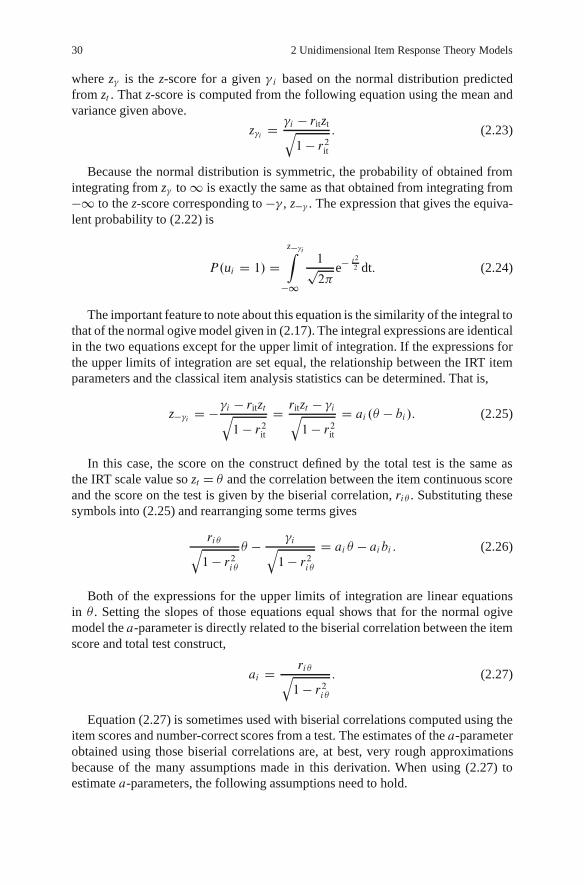
30 2 Unidimensional Item Response Theory Models
where z� is the z-score for a given �i based on the normal distribution predictedfrom zt . That z-score is computed from the following equation using the mean andvariance given above.
z�i D �i � ritztq1 � r2it
: (2.23)
Because the normal distribution is symmetric, the probability of obtained fromintegrating from z� to 1 is exactly the same as that obtained from integrating from�1 to the z-score corresponding to �� , z�� . The expression that gives the equiva-lent probability to (2.22) is
P.ui D 1/ Dz��iZ
�1
1p2�
e� t2
2 dt: (2.24)
The important feature to note about this equation is the similarity of the integral tothat of the normal ogive model given in (2.17). The integral expressions are identicalin the two equations except for the upper limit of integration. If the expressions forthe upper limits of integration are set equal, the relationship between the IRT itemparameters and the classical item analysis statistics can be determined. That is,
z��i D ��i � ritztq1 � r2it
D ritzt � �iq1 � r2it
D ai .� � bi/: (2.25)
In this case, the score on the construct defined by the total test is the same asthe IRT scale value so zt D � and the correlation between the item continuous scoreand the score on the test is given by the biserial correlation, ri� . Substituting thesesymbols into (2.25) and rearranging some terms gives
ri�q1 � r2i�
� � �iq1 � r2i�
D ai � � aibi : (2.26)
Both of the expressions for the upper limits of integration are linear equationsin � . Setting the slopes of those equations equal shows that for the normal ogivemodel the a-parameter is directly related to the biserial correlation between the itemscore and total test construct,
ai D ri�q1 � r2i�
: (2.27)
Equation (2.27) is sometimes used with biserial correlations computed using theitem scores and number-correct scores from a test. The estimates of the a-parameterobtained using those biserial correlations are, at best, very rough approximationsbecause of the many assumptions made in this derivation. When using (2.27) toestimate a-parameters, the following assumptions need to hold.

2.1 Unidimensional Models of the Interactions of Persons and Test Items 31
1. The regression of the item z-score on the test z-score is linear.2. Errors of estimation in the prediction of item scores from test scores are normally
distributed.3. The standard deviation of the distributions of errors of prediction of the items
scores from the test scores is constant over the range of the �-values.4. All persons above the point where the item continuous scale is dichotomized will
answer the item correctly.5. The biserial correlation between the item score and total score is a good estimator
of the correlation between the continuous item score and total score.
Although the estimates of the a-parameters given by (2.27) may not be very precise,the derivation does indicate that there is a fairly strong relationship between thebiserial correlation and the a-parameter, even if it is not a mathematical function.
Another statistic that is sometimes used as a measure of the discriminating powerof a test item is the loading of the test item on the first common factor of the item set.When the test is composed of items that are dichotomously scored, the analysis isoften performed on the matrix of inter-item tetrachoric correlations. Because the useof tetrachoric correlations is based on the same assumptions as those underlying thebiserial correlation (i.e., the underlying item construct is normally distributed anddichotomized at a point on the construct scale), the argument relating the biserialcorrelation to the a-parameter for a test item works equally well for item factorloadings. In fact, the argument is even stronger because the factor loading is thecorrelation between the item construct and the score on the first common factorrather than the number-correct score on the test. The former is a better estimateof � than is the number-correct score because it is an estimate of the latent variableunderlying the item responses and it is on the z-score scale. The relationship betweenthe a-parameter for an item and its factor loading is given by an equation that is thedirect analog to (2.27) with all of the same concerns about whether all of the listedassumptions apply. The equation is
ai D �iq1 � �2i
; (2.28)
where �i is the loading of Item i on the first common factor from the set of items onthe test.
2.1.2.3 Lower Asymptote
The lower asymptote parameter that is represented by c in (2.13) and (2.17) does nothave a direct counterpart in traditional item analysis. This parameter indicates theproportion of examinees that will respond correctly to the test item as the ability ofthe examinee approaches �1. Some item analysis programs do provide informationthat can be used to approximate the c-parameter. These programs report the numberof examinees choosing each response alternative in the multiple-choice item for

32 2 Unidimensional Item Response Theory Models
groups of examinees at different performance levels defined on the total score forthe test as a whole. For example, the analysis sample may be divided into fifthsfrom the top fifth to the bottom fifth based on the number-correct score on the test.Then, the proportion choosing each alternative can be computed for each fifth ofthe sample. Typically, the proportion choosing the correct answer will decline as theoverall performance level of the examinee groups decline. The proportion choosingthe correct answer in the lowest group is an estimate of the c-parameter.
Many early descriptions of IRT models labeled the c-parameter as the guessingparameter because it was expected that it would generally be equal to 1=m, wheremis the number of response alternatives for the multiple-choice question. This is theproportion of correct responses that would be expected if the examinees chose re-sponses totally at random. Empirical estimates of the c-parameter (see Lord 1980 forsome examples) are often less than 1=m suggesting that c is not a random guessingparameter. It is more accurately described as a parameter that describes the perfor-mance of examinees with low trait levels. In this book, the latter interpretation isaccepted and the c-parameter is referred to as the lower asymptote parameter.
2.1.3 Models for Items with More Than Two Score Categories
Although the majority of the work on IRT models has concentrated on the analy-sis of data from test items with two scores – 0 and 1, there has been a significantamount of development work on items that have more than two score categories.These models are designed for modeling the interaction of persons with of a vari-ety of types of test items such as writing samples, open ended mathematics items,and rating scale responses to survey questions. Because the actual response activityfor these different types of items are different – generating writing samples, solv-ing mathematics problems, rating statements – the IRT models that describe theitem/persons interactions with them are different as well. The characteristics of avariety of these models are described in van der Linden and Hambleton (1997) andvan der Ark (2001), so they will not be repeated here. Most of the work on thegeneralizations of these models to the multidimensional case has focused on threeof them – the partial credit model (Masters 1982) and the generalized partial creditmodel (Muraki 1992) and the graded response model (Samejima 1969). The uni-dimensional versions of these models are described here and the multidimensionalversions are presented in Chap. 4.
2.1.3.1 The Partial Credit Model
The partial credit model (Masters 1982; Masters and Wright 1997) is a mathematicalform that was designed for test items with two or more ordered categories. Thepartial credit model is appropriate for test items that are believed to require thesuccessful accomplishment of a number of tasks. To receive the maximum score on

2.1 Unidimensional Models of the Interactions of Persons and Test Items 33
the item, all of the tasks need to be correctly completed. The partial credit model isappropriate for open-ended items when scorers consider many different componentsof the response and score each of them as correct/incorrect or accomplished/notaccomplished. The score for the test item as a whole is the number of componentsthat were successfully completed (Verhelst and Verstralen 1997).
The scores on the item represent levels of performance, with each higher scoremeaning that the examinee accomplished more of the desired task. The boundariesbetween adjacent scores are labeled thresholds and an examinee’s performance ison either side of a threshold with a particular probability. The scoring scale for theitem can be dichotomized at each threshold and the model specifies the probabilityof a response in the categories above or below the selected threshold. This can bedone for each threshold.
The mathematical expression for the partial credit model is given by
P.uij D k j �j / D e
"kP
uD0
.�j�ıiu/
#
miP
vD0e
"vP
uD0.�j�ıiu/
# ; (2.29)
where k is the score on Item i , mi is the maximum score on Item i , and ıiu is thethreshold parameter for the uth score category for Item i .
For purposes of keeping notation less complex,
0X
uD0.�j � ıiu/ � 0 and
kX
uD0.�j � ıiu/ �
kX
uD1.�j � ıiu/: (2.30)
Note that the simplifying expressions in (2.30) indicate that the value of ıi0 has noimpact on the model. No matter what value is chosen for this parameter, the termin the summation associated with it will have a value of 0. Often this parameter isset equal to 0 as a convenience, but that does not mean that there is a 0 threshold.The other ıiu parameters specify the thresholds between score categories. This canbe seen in (2.7) that shows the probability of each score as a function of � .
The score characteristic functions shown in Fig. 2.7 are for a test item that hasfour score categories �0, 1, 2, 3. The curves in the figure show the probability ofeach score category for a person at a specific �-level. For example, if � is equal to�1, the probability of a score of 0 is .07, a score of 1 is .54, a score of 2 is .36, anda score of 3 is .03. A score of 1 is the most likely score at the �-level, but the otherscores are also possible.
The threshold parameters indicate where the adjacent score categories have equallikelihoods. Scores of 0 and 1 have equal likelihoods at �3. Scores of 1 and 2 haveequal likelihoods at �:5. These threshold points are places where the curves foradjacent score categories cross. For this item, the threshold parameter values arein order from low to high (ignoring the 0 place holder value). This ordering of

34 2 Unidimensional Item Response Theory Models
–4 –3 –2 –1 0 1 2 3 40
0.1
0.2
0.3
0.4
0.5
0.6
0.7
0.8
0.9
1
θ
Prob
abili
ty
P(u=0)P(u=1)P(u=2)P(u=3)
Fig. 2.7 Score category probabilities for an item with ı-parameters 0, �3, �:5, 1.5
–4 –3 –2 –1 0 1 2 3 40
0.1
0.2
0.3
0.4
0.5
0.6
0.7
0.8
0.9
1
θ
Prob
abili
ty P(u=0)P(u=1)P(u=2)P(u=3)
Fig. 2.8 Score category probabilities for an item with ı-parameters 0, �:5, �3, 1.5
threshold parameters is not a requirement of the model. Figure 2.8 shows the scorecharacteristic functions for a test item with threshold parameters that have the samenumerical values, but in different order – �:5, �3, 1.5. For this case, the probabilityof a score 1 for a person at �1 on the �-scale is much lower than for the previousitem – approximately .1. For this item, a score of 1 is never the most likely response.The model is indicating that this is a seldom used score category and it might bemore reasonable to consider this a three category item.

2.1 Unidimensional Models of the Interactions of Persons and Test Items 35
The expected score on the item as a function of level on the �-scale is specified by
E.uij j �j / DmiX
kD0kP.uij D k j �j /: (2.31)
The expected score ranges from 0 to mi as a function of � . The expected scoreon the item has an equivalent interpretation to the ICC for dichotomously scoreditems. The expected score functions for the examples shown in Figs. 2.7 and 2.8 aregiven in Fig. 2.9. The curves have a different form because of the different orderingof the threshold parameters. Example 2 increases quickly from 0 to 2 because theprobability of a score of 1 is very low. As for dichotomously scored items, the curvesindicate easy items if they are far to the left and hard items if they are far to the right.
The partial credit model is a member of the Rasch family of item response mod-els. Masters and Wright (1997) indicate that when the item is only considered toconsist of two adjacent score categories, the resulting model is the Rasch model fordichotomous items. That is, using the notation defined above,
P.uij D k j �j /P.uij D k � 1 j �j /C P.uij D k j �j / D e.�j�ıik/
1C e.�j�ıik/; k D 1; 2; : : : ; mi :
(2.32)
The expression on the right is the Rasch model for dichotomous items withthe threshold parameter as the difficulty parameter. This model fits the adjacentscore categories using the Rasch model for dichotomous items indicating that all of
–4 –3 –2 –1 0 1 2 3 40
0.5
1
1.5
2
2.5
3
θ
Expe
cted
Sco
re
Example 1Example 2
Fig. 2.9 Expected score curves for the two example items

36 2 Unidimensional Item Response Theory Models
–4 –3 –2 –1 0 1 2 3 40
0.1
0.2
0.3
0.4
0.5
0.6
0.7
0.8
0.9
1
θ
Prob
abili
ty
Threshold 0-1Threshold 1-2Threshold 2-3
Fig. 2.10 Adjacent score characteristic curves for thresholds �3, �:5, 1.5
the distinctions between score categories have the same slope at the point of inflec-tion and the point of steepest slope for the curves for distinguishing the responsefunctions is at the �-value corresponding to the threshold value. The curves foradjacent score pairs for the first example item are shown in Fig. 2.10.
It is easily seen in Fig. 2.10 that the .5 probability line intersects the curves atthe values on the �-scale equal to the threshold parameters. Also, the curves donot intersect and have the same slope where they cross the .5 probability line. Fur-ther, the slope at the point of inflection is the same as that for the Rasch model fordichotomous items – .25.
2.1.3.2 The Generalized Partial Credit Model
The generalized partial credit model (Muraki 1992) is an extension of the partialcredit model proposed by Masters (1982). The extension is the addition of the dis-crimination parameter, a, to the partial credit model. This is similar conceptually tothe relationship between the one-parameter logistic model and the two-parameterlogistic model. Although the partial credit model is a member of the family ofRasch models because it has observable sufficient statistics for the item and per-son parameters, the generalized partial credit model is not. The addition of thediscrimination parameter allows variation in the discriminating power of items tobe modeled. However, adding a discrimination parameter that is estimated as partof item calibration removes the generalized partial credit model from the family ofRasch models.

2.1 Unidimensional Models of the Interactions of Persons and Test Items 37
Like the partial credit model, the generalized partial credit model is appropriatefor test items that are considered to require the successful accomplishment of anumber of tasks. To receive the maximum score on the item, all of the tasks need tobe correctly completed. The generalized partial credit model is appropriate for open-ended items scored considering many different components of the response. Eachcomponent is scored as correct/incorrect or accomplished/non accomplished. Thescore for the test item as a whole is the number of components that were successfullycompleted (Verhelst and Verstralen 1997).
The scores on the item represent levels of performance, with each higher scoremeaning that the examinee accomplished more of the desired task. As with the par-tial credit model, the boundaries between adjacent scores are labeled thresholds andan examinee’s performance is on either side of a threshold with a particular prob-ability. The score scale for the item can be dichotomized at each threshold and themodel specifies the probability of being in each of the two resulting categories. Thiscan be done for each threshold.
The mathematical expression for the generalized partial credit model is givenbelow
P.uij D k j �j / D e
"kP
uD1
Dai .�j�biCdiu/
#
miP
vD1e
"vP
uD1Dai .�j�biCdiu/
# ; (2.33)
where k is the score on the item, mi is the total number of score categories for theitem, diu is the threshold parameter for the threshold between scores u and u�1,and all of the other symbols have their previous definitions. Note that di1 is definedas 0. This model has a parameter bi that indicates the overall difficulty of the testitem and a parameter ai that indicates the overall discrimination power of the item.The discrimination power is assumed to be the same at all thresholds, but ai maydiffer across items. The threshold parameters, dik, indicate where the likelihood ofresponses changes from being greater for response category k� 1 to being greaterfor response category k. For estimation purposes, the sum of the dik-parameters isusually constrained to sum to 0.
The parameterization used in the PARSCALE program (Muraki and Bock 1991)is used in (2.33). If the a-parameter is set equal to 1=D for all items and ıiu D bi �diu, the result is the partial credit model in (2.29). Note that the index of summationalso starts at 0 instead of 1. If the a-parameter is .588 (i.e., 1/1.7), the b-parameteris 0, and the d -parameters are 3, .5, �1:5, the score category probability curves arethe same as those shown in Fig. 2.7.
To show the effects of the discrimination parameter on the form of the functionsdescribing the interactions between persons and an item whose characteristics canbe represented by the generalized partial credit model, the score category probabilitycurves are shown for two item – one with a D :5 and the other with a D 1:5. Bothitems have b D �:5, and d -parameters 0, 3, �1, �2. The curves for each scorecategory, 1, 2, 3, 4, are shown in Fig. 2.11 with the solid lines representing the itemwith a D :5 and the dashed lines representing the item with a D 1:5. It is clear that

38 2 Unidimensional Item Response Theory Models
–4 –3 –2 –1 0 1 2 3 40
0.1
0.2
0.3
0.4
0.5
0.6
0.7
0.8
0.9
1
θ
Prob
abili
ty
Fig. 2.11 Generalized partial credit model score probability curves for b D �:5, ds D 0, 3, �1,�2, and a D :5 (solid curves) and 1.5 (dashed curves)
the probabilities for each score category change more quickly when a has a highervalue. Also, the curves for adjacent score categories cross at the same value of � –the value of the corresponding threshold bi � diu.
The score curves for obtaining the higher of adjacent score categories can beobtained in the same way as for the partial credit model. These curves for a D :5
(solid lines) and 1.5 (dashed lines) are shown in Fig. 2.12. The curves for the samescore categories cross the .5 probability line at the same points – the values ofthe thresholds. The slopes of the lines where they cross the .5 probability line arethe same as for the two-parameter logistic model – Da/4. The slopes are all the samewithin item, but they differ across the two items.
2.1.3.3 Graded Response Model
The graded response model (Samejima 1969) is designed for test items that havesomewhat different requirements than the partial credit models. The partial creditmodels consider the items to have a number of independent parts and the score indi-cates how many parts were accomplished successfully. The graded response modelconsiders the test item to require a number of steps but the successful accomplish-ment of one step requires the successful accomplishment of the previous steps. Ifstep k is accomplished, then previous steps are assumed to be accomplished as well.
The parameterization of the model given here considers the lowest score on Itemi to be 0 and the highest score to be mi . The probability of accomplishing k ormore steps is assumed to increase monotonically with an increase in the hypothetical

2.1 Unidimensional Models of the Interactions of Persons and Test Items 39
–4 –3 –2 –1 0 1 2 3 40
0.1
0.2
0.3
0.4
0.5
0.6
0.7
0.8
0.9
1
θ
Prob
abili
ty
Fig. 2.12 Score characteristic curves for adjacent response categories for a D :5 (solid curves)and a D 1:5 (dashed curves)
construct underlying the test, � . The probability of accomplishing k or more stepsis typically represented as a two-parameter normal ogive or logistic model. Theprobability of receiving a specific score, k, is the difference between the probabilityof doing the work for k or more steps and doing the work for k C 1 or more steps.If the probability of performing the work including step k at a particular �-level isP �.uij D k j ™j/, then the probability that an examinee will receive a score of k is
P.uij D k j �j / D P �.uij D k j �j / � P �.uij D k C 1 j �j /; (2.34)
where P �.uij D 0j�j/ D 1 because doing the work for step 0 or more is a cer-tainty for all examinees and P �.uij D mi C 1j�j/ D 0 because it is impossibledo work representing more than category mi . The latter probability is defined sothat the probability of each score can be determined from (2.34). Samejima (1969)labels the terms on the right side of the expression as the cumulative category re-sponse functions and those on the left side of the expression as the category responsefunction.
The normal ogive form of the graded response model is given by
P.uij D k j �j / D 1p2�
ai .�j�bik/Z
ai .�j�bi;kC1/
e�t2
2 dt; (2.35)
where k is the score on the item, 0; 1; : : :; mi , ai is an item discrimination parameter,and bik is a difficulty parameter for the kth step of the item.

40 2 Unidimensional Item Response Theory Models
Using the same symbols, the logistic form of the model is given by
P.uij D k j �j / D eDai .�j�bik/ � eDai .�j�bi;kC1/
.1C eDai .�j�bik//.1C eDai .�j�bi;kC1//: (2.36)
Note that this form of the model includes the constant,D D 1:7, so that the param-eterization of the logistic version of the model will be very similar to that for thenormal ogive version of the model.
The cumulative category response functions for the logistic form of the gradedresponse model with step difficulty parameters bik D �2, �1, .7, and 2 and dis-crimination parameter ai D 1 are presented in Fig. 2.13. The curves are the sameas the two-parameter logistic model for dichotomously scored items. They cross the.5-probability line at a point equal to the step difficulty and their slopes are steepestat that point. All of the curves have the same slope at their points of inflection, ai =4.
The probabilities of each of the five response categories, 0, 1, 2, 3, and 4 for thisitem can be determined from (2.34). The probabilities of each response conditionalon level of � are given by the category response functions in Fig. 2.14. The curvecorresponding to the score of 0 is a decreasing function of � and it crosses the .5-probability line at the value of bi1, �2. The curve corresponding to the highest scorecategory, mi D 4, crosses the .5-probability line at bi4, 2. The other curves do nothave an obvious relationship to the item parameters. The intersection points of thecurves are not equal to the b-parameters as they are for the partial credit model.
The effect of changes to the a-parameters can be seen in Figs. 2.15a and b.Figure 2.15a shows the probability in each response category for the test item shown
–4 –3 –2 –1 0 1 2 3 40
0.1
0.2
0.3
0.4
0.5
0.6
0.7
0.8
0.9
1
θ
Prob
abili
ty
Prob 1-4Prob 2-4Prob 3-4Prob 4
Fig. 2.13 Cumulative category response functions for an item modeled by the logistic version ofthe graded response model with ai D 1 and bik’s D �2, �1, .7, 2.

2.1 Unidimensional Models of the Interactions of Persons and Test Items 41
–4 –3 –2 –1 0 1 2 3 40
0.1
0.2
0.3
0.4
0.5
0.6
0.7
0.8
0.9
1
θ
Prob
abili
ty
Prob 0Prob 1Prob 2Prob 3Prob 4
Fig. 2.14 Category response functions for an item modeled by the logistic version of the gradedresponse model with ai D 1 and bik’s D �2, �1, .7, 2
–4 –2 0 2 40
0.1
0.2
0.3
0.4
0.5
0.6
0.7
0.8
0.9
1
θ
Prob
abili
ty
a
–4 –2 0 2 40
0.1
0.2
0.3
0.4
0.5
0.6
0.7
0.8
0.9
1b
θ
Fig. 2.15 Category response functions for items modeled by the logistic version of the gradedresponse model with (a) ai D 1 (solid lines) and 1.5 (dashed lines), and bik’s D �2, �1, .7, 2 and(b) ai D 1 (solid lines) and 1.5 (dashed lines), and bik’s D �2, �1, .7, 2 (solid lines) and �1:5,�:5, 1.2, 2.5 (dashed lines)
in Fig. 2.14 and an item with the same b-parameters, but with the ai -parameter equalto 1.5. The graphs show that the increase in ai -parameter from 1 to 1.5 results insteeper curves for the extreme score categories, and more peaked curves for the cat-egories between the extremes. The curves for the extreme categories still cross the
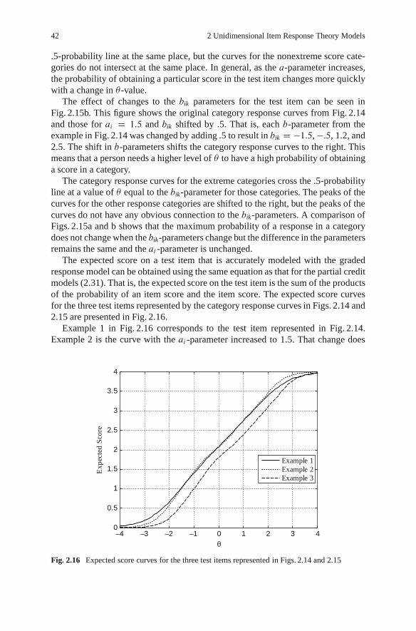
42 2 Unidimensional Item Response Theory Models
.5-probability line at the same place, but the curves for the nonextreme score cate-gories do not intersect at the same place. In general, as the a-parameter increases,the probability of obtaining a particular score in the test item changes more quicklywith a change in �-value.
The effect of changes to the bik parameters for the test item can be seen inFig. 2.15b. This figure shows the original category response curves from Fig. 2.14and those for ai D 1:5 and bik shifted by .5. That is, each b-parameter from theexample in Fig. 2.14 was changed by adding .5 to result in bik D �1:5, �:5, 1.2, and2.5. The shift in b-parameters shifts the category response curves to the right. Thismeans that a person needs a higher level of � to have a high probability of obtaininga score in a category.
The category response curves for the extreme categories cross the .5-probabilityline at a value of � equal to the bik-parameter for those categories. The peaks of thecurves for the other response categories are shifted to the right, but the peaks of thecurves do not have any obvious connection to the bik-parameters. A comparison ofFigs. 2.15a and b shows that the maximum probability of a response in a categorydoes not change when the bik-parameters change but the difference in the parametersremains the same and the ai -parameter is unchanged.
The expected score on a test item that is accurately modeled with the gradedresponse model can be obtained using the same equation as that for the partial creditmodels (2.31). That is, the expected score on the test item is the sum of the productsof the probability of an item score and the item score. The expected score curvesfor the three test items represented by the category response curves in Figs. 2.14 and2.15 are presented in Fig. 2.16.
Example 1 in Fig. 2.16 corresponds to the test item represented in Fig. 2.14.Example 2 is the curve with the ai -parameter increased to 1.5. That change does
–4 –3 –2 –1 0 1 2 3 40
0.5
1
1.5
2
2.5
3
3.5
4
θ
Exp
ecte
d Sc
ore
Example 1Example 2Example 3
Fig. 2.16 Expected score curves for the three test items represented in Figs. 2.14 and 2.15

2.2 Other Descriptive Statistics for Items and Tests 43
not have a dramatic effect on the expected score curve. The curve is somewhatsteeper when � is high or low, but the two curves are almost indistinguishable inthe �s in the range from �2 to 2. Example 3 is the curve for the test item with thebik-parameters shifted up by .5. It is clear that the shift in the bik-parameters movesthe curve to the right. This indicates that a higher �-value is needed for this testitem to have the same expected score as for Example 2. To have that same expectedscore, the �-value must be increased by .5. The curves in Fig. 2.16 do not match thenormal ogive or logistic forms. They have changes in curvature along the range of �that results from differences in the distance between the bik-parameters. The slopeof the curve changes along the range of � depending on the distance between thebik-parameters.
2.2 Other Descriptive Statistics for Items and Tests
Along with the item parameters for the UIRT models, there are several statistics thatdescribe the function of items and tests that are unique to IRT. These statistics arederived from the IRT models to further describe what the item response data tellabout the item/person interactions. The most commonly used of these statistics arethe expected summed score on a test composed of a set of items and the amountof information about the location of an examinee provided by the response to atest item or a collection of test items. These statistics can be computed as singledescriptive values, but they are usually computed for all levels of � . When this isdone, they are functions of � rather than single values. The expected summed scorefunction, usually called a test characteristic curve, and the information function aredescribed in this section.
2.2.1 The Test Characteristic Curve
Regression analysis is a methodology that is quite frequently used to predict thevalue of one variable from the value of another variable. For example, the value ofa variable y can be predicted from the value of another variable x. The prediction ismade so that error is minimized. Regression procedures were originally developedwith error defined as the squared difference between the observed value of y andthe predicted value of y. In that case, the expected value of y conditional on thepredictor value x is used as the predicted value of y.
In the context of IRT, the variable that is usually predicted is the scored responseto the test item. This item score is predicted from the value of � . A regression pre-dictor of the item score from � is given by the expected value of the item scoreconditional on the value of � , E.uj�/. For an item with two score categories, 0 and1, the regression predictor of the item score from � is given by
E.u j �/ D 1P.u D 1 j �/C 0P.u D 0 j �/ D P.u D 1 j �/; (2.37)

44 2 Unidimensional Item Response Theory Models
where all of the symbols have been defined previously. Equation (2.37) shows thatthe regression of the item score on � is the same as the IRT function for the proba-bility of correct response to the item when the test item has a score of 0 or 1. Whentest items have more than two score categories, the regression of the item score on� is not quite as simple. For polytomously scored test items, the regression of theitem score on � is given by (2.31).
A traditional method for scoring tests has been to compute the sum of theitem scores. This score is often called the total score, the raw score or the number-correct score. Because tests often have combinations of dichotomously and poly-tomously scored items, the term “number-correct” does not accurately describethese cases. The term “summed score” will be used here as a synonym for all ofthese terms that accurately reflects how these scores are produced. That is, the term“summed score” will refer to an unweighted sum of the item scores.
The regression of the summed score on � is the expected value of the summedscore conditional on � . If the summed score for a person is represented by yj, theregression predictor of yj from �j is given by
E.yj j �j / D E
nX
iD1uij j �j
!
DnX
iD1E.uij j �j /; (2.38)
where n is the number of items on the test. For the special case of a test composedof items that are scored 0 or 1 the expression on the left of (2.38) is simply the sum
of the item characteristic functions for the test items,nP
iD1P.uij j �j /.
The plot of the expected value of the summed score against � is typically referredto as the test characteristic curve (TCC). Because classical test theory defines thetrue score on a test as the expected value of the observed score yj (see Lord andNovick 1968), the TCC shows the relationship between the true score from classicaltest theory and the � from item response theory. Lord (1980) considers true scoreand � as representing the same concept, but being monotonic transformations ofeach other.
The TCC for a set of items appears in the psychometric literature in two dif-ferent forms. One form is a plot with the horizontal axis representing � and thevertical axes representing the expected summed score. This is a direct representa-tion of (2.38). Sometimes, it is more useful to transform the TCC to use a proportionof maximum possible score (proportion correct for tests with items scored 0 or 1).That is, the expected summed score is divided by the maximum possible summedscore. For that case, the vertical axis has a range from 0 to 1. This representationis more convenient when it is desired to compare TCCs from tests with differentnumbers of test items. Examples of the two representations of TCCs are given inFig. 2.17. The item parameters used to produce the TCCs are given in Table 2.1.Table 2.1 contains item parameters for a set of 50 multiple choice and open endeditems that are scored as either correct (1) or incorrect (0). The item parameters arefor the three-parameter logistic model when the items are multiple-choice and for

2.2 Other Descriptive Statistics for Items and Tests 45
Fig. 2.17 Test characteristic curve (TCC) for items in Table 2.1
Table 2.1 Item parameters for 50 dichotomously score test items
Item a b c Item a b cnumber number
1 1.83 0:91 0 26 1.44 0:58 0:27
2 1.38 0:81 0 27 2.08 0:82 0
3 1.47 0:06 0 28 0.81 �0:22 0:20
4 1.53 �0:80 0:25 29 1.10 1:82 0:23
5 0.88 0:24 0:21 30 0.66 0:26 0
6 0.82 0:99 0:29 31 0.91 �0:97 0:20
7 1.02 1:23 0:26 32 0.61 0:08 0:22
8 1.19 �0:47 0:19 33 0.67 0:54 0:17
9 1.15 2:78 0 34 0.43 1:22 0:20
10 0.18 �3:85 0:21 35 0.70 �1:27 0
11 0.70 1:49 0 36 0.83 1:02 0:13
12 1.36 0:56 0:20 37 1.30 1:50 0:18
13 1.53 0:80 0:21 38 2.01 1:19 0:28
14 1.17 �0:29 0:18 39 1.02 �0:68 0:20
15 1.14 �1:05 0:19 40 1.60 1:83 0:24
16 0.94 �0:25 0:15 41 1.02 �0:69 0:21
17 1.64 1:14 0:29 42 0.96 0:23 0:26
18 1.21 0:43 0:13 43 1.45 0:78 0:21
19 1.67 0:27 0:26 44 1.48 1:22 0:13
20 0.67 �0:32 0:19 45 2.23 1:64 0
21 1.74 1:99 0:29 46 1.51 0:24 0:17
22 0.74 0:59 0:19 47 0.88 0:58 0:12
23 0.79 �0:28 0:14 48 0.78 �0:06 0:24
24 1.38 1:06 0:15 49 0.52 �0:10 0
25 1.84 0:90 0:09 50 0.97 1:38 0
The zeros in the c columns indicate that short answer items were assumed to have a zero probabilityfor guessing a correct response

46 2 Unidimensional Item Response Theory Models
the two-parameter logistic model when the items are short-answer scored correct orincorrect. The c-parameters for the short-answer items are shown as 0 in the tablebecause there was assumed to be no chance of guessing the answer to these items.
The left panel of Fig. 2.17 shows the TCC for this set of items with the summedscore on the vertical axis. The appearance of this curve is similar to that of an ICC fora three-parameter logistic model, but the curve can not be modeled by that functionunless all of the test items have the same item parameters. The possible forms ofthe TCC are quite varied. Lord and Novick (1968) provide informative examples inChap. 16. The TCC in Fig. 2.17 has a lower asymptote that is equal to the sum ofthe c-parameters, 7.938. The TCC tends to be steepest for a value of the expectedsummed score of 29 that is half way between the lower asymptote and the maximumpossible summed score. This is approximately the case for sets of test items that havea unimodal distribution of difficulty, but it is not a mathematical necessity. For setsof test items that have a bimodal distribution of difficulty, the TCC can have a lowerslope in the middle range than for higher or lower values.
The right panel of Fig. 2.17 shows the TCC (dark line) using the proportion ofmaximum possible summed score as the vertical axis. The figure also contains theICCs for all 50 items. When using the proportion of maximum possible as the verti-cal axis, the TCC is the average of all of the ICCs. A comparison of the two panelsin the figure will show that the TCCs have exactly the same form – it is only thenumerical values on the vertical axis that differ.
The TCC always shows a nonlinear relationship between � and the expectedsummed score because the summed score has a finite range and � has an infiniterange. Where the TCC is fairly flat, the test is mapping a broad range of the �-scaleinto a narrow range of the summed score scale. For example, the � range from �4to �2 is mapped into the summed score range from 8 to 10. Wherever the TCC issteep, the opposite is the case – the test provides a spread of summed scores for afairly narrow range of the �-scale. For the example given here, the �-range from 1to 1.5 is mapped into the range from 34 to 40 on the summed-score scale.
The TCC can be used to determine the shape of the expected summed-score dis-tribution, that is, the true score distribution, when the �-distribution is known. TheTCC provides the transformation that maps the area within given boundaries on the�-scale to the corresponding boundaries on the summed-score scale. Figure 2.18provides an example of the estimation of the true score distribution. The TCC shownin the figure is computed from the item parameters in Table 2.1. The � distributionis assumed to be normal with a mean 0 and standard deviation 1. The left panelof the figure shows the estimated true score distribution for the summed scoresbased on the assumed � distribution and TCC. Note that the true score distributionis positively skewed because the majority of the b-parameters are positive indicat-ing that the test is fairly difficult. Also, there are no scores below the sum of thec-parameters because this is a true score distribution – the scores are the expectedscores for a particular level of � and it is not possible to get a expected score lessthan the sum of the chance levels. Any assumed distribution of � can be mappedthrough the TCC to determine the corresponding true score distribution. Lord and

2.2 Other Descriptive Statistics for Items and Tests 47
00.050
10
20
30
40
50
Probability
Sum
med
Sco
re
–4 –2 0 2 4
–4 –2 0 2 4
0
0.1
0.2
0.3
0.4
θ
Den
sity
Fig. 2.18 True score distribution estimated from � distribution using the TCC
Novick (1968, pp. 386–392) provide examples using a number of different TCCsand � distributions. Lord (1980) shows how to estimate the observed summed-scoredistribution as well as the true summed-score distribution.
2.2.2 Information Function
The term “information” as it is used in IRT is a statistical indicator of the qual-ity of the estimate of a parameter, usually the trait parameter that is the target forthe test. Because item responses provide information for all levels of values on the�-scale, information is usually represented as a function of the parameter being esti-mated rather than as a single value. The formula for information can be derived in anumber of different ways. Birnbaum (1968) showed that the value of information isrelated to the length of the confidence interval around the trait estimate for a person.Kendall and Stuart (1961) indicated that the information function is related to theasymptotic standard error of the maximum likelihood estimate of the trait parameter.The approach taken here is to show that the information function is an indicator ofthe degree to which the reported score from a test or item differentiates between realdifferences in the trait of interest. In effect, the information function indicates howmany standard errors of the trait estimate are needed to equal one unit on the �-scale.When more standard errors are needed to equal one unit on the �-scale, the standarderrors are smaller indicating that the measuring instrument is sensitive enough to

48 2 Unidimensional Item Response Theory Models
detect relatively small differences in � . This approach to defining information is acombination of conceptual definitions of information provided by Lord (1980) andHambleton and Swaminathan (1985).
Suppose the trait of interest can be assessed using a test composed of test itemsthat can be accurately modeled by a unidimensional IRT model and that the true traitlevel for a person is given by �j. The true trait level of a person can not be observed.Rather, the observed score on a test for person j is represented by an estimate yj. Ifit were possible to administer the test to the person repeatedly and get independentestimates of yj, it would not be expected that all of the estimates would be the same.Instead, the yj would vary and the full set of estimates could be collected togetherto form a distribution that would have a mean and standard deviation. The meanfor a person with trait level �j is indicated by �y j �j . The standard deviation of thedistribution is indicated by �y j �j . This standard deviation is called the conditionalstandard error of measurement of test score y in classical test theory.
Now suppose that two individuals with different levels of � are assessed usingthe same test and that the sensitivity of the test to differences in their trait level is ofinterest. A useful measure of the sensitivity of the test is given by
�y j �2 � �y j �1�y j �1;�2
; (2.39)
where �y j �1;�2 is the pooled standard error of measurement at the two � values.This measure of sensitivity indicates the distance between the means of the sam-
pling distributions for the two individuals in terms of standard error units. If theresult were 1.7, it would mean that the expected observed scores for the two indi-viduals were 1.7 standard error units apart. Of course the value given by (2.39) isdependent on the distance between �1 and �2. If the distance between the two indi-viduals is greater, the number of standard errors units they are apart will be greateras well. To compare the sensitivity of the test for distinguishing between individualsat different places in the �-scale, an index is needed that is comparable – one thatrefers to the same distance on the �-scale. Such an index can be developed by divid-ing the expression in (2.39) by the difference in �-values. This results in a measurethat tells the number of standard error units corresponding to one unit on the �-scale.The resulting expression is
�y j �2��y j �1
�y j �1;�2
�2 � �1 D �y j �2 � �y j �1�y j �1;�2 .�2 � �1/
: (2.40)
Thus, if the result from (2.39) was 1.7 and the two persons were .5 unit apart onthe �-scale, the result would be 3.4 – the projected number of standard error units forpersons one unit apart on the �-scale. This index is based on an assumption that thedistance between individuals on the expected observed score scale increases linearlywith increase in distance on the �-scale. Although this is a good approximationwhen �-values are close together, a review of typical test characteristic curves showsthat it is not true in general. To avoid this assumption of a linear relationship, a

2.2 Other Descriptive Statistics for Items and Tests 49
measure of sensitivity for each value of � is needed rather than one for each pairof �-values. This measure can be obtained by taking the limit of the expression in(2.40) as �1 approaches �2. When �1 and �2 are very close to each other, the pooledstandard error is approximately the same as the conditional standard error at thatpoint on the �-scale. Equation (2.40) then becomes
lim�1!�2
��y j �2 � �y j �1�y j �1;�2 .�2 � �1/
�D
@�y j �
@�
�y j �: (2.41)
Values of the expression in (2.41) are functions of � . They indicate how welldifferences in � can be detected using the test items that produce the observed score,y. The value at a particular level of � tells how far apart in standard error units arethe observed scores that correspond to a one unit difference on the �-scale at thepoint defined by the given value of � .
Lord (1980), as well as other researchers, has shown that when the maximumlikelihood estimator of � is used as the reported score for a test, then the recipro-cal of the square of the function given in (2.41) is equal to the asymptotic varianceof the maximum likelihood estimate. The squared value of the function is calledthe amount of information provided by the estimate about the true value of � .While some researchers initially preferred the values directly from (2.41) (e.g.,Samejima 1982), most texts now call the square of the expression the informationfunction for the scoring formula y. The function is indicated by
I.�; y/ [email protected] j �/@�
i2
�2y j �
: (2.42)
When the observed score of interest is the 0,1-score on a single dichotomous testitem, the information function simplifies to
I.�; ui / Dh@Pi .�/
@�
i2
Pi .�/Qi .�/; (2.43)
where ui is the score for Item i , Pi.�/ is the probability of correct response for theitem, and Qi.�/ D 1–Pi .�/. When the three-parameter logistic model accuratelyrepresents the interaction between the persons and test items, (2.43) becomes
I.�; ui / D a2iQi .�/
Pi .�/
�Pi.�/� ci
1 � ci
�2: (2.44)
When ci D 0, this expression gives the information for the two-parameter logisticmodel, and in addition if ai D 1, then the expression simplifies to the informationfunction for the Rasch one-parameter logistic model. To show the effects of theparameters on the information function, the functions are shown graphically for

50 2 Unidimensional Item Response Theory Models
–4 –3 –2 –1 0 1 2 3 40
0.1
0.2
0.3
0.4
0.5
0.6
0.7
θ
Info
rmat
ion
Item 1Item 2Item 3
Fig. 2.19 Information functions for items following the Rasch, 2pl, and 3pl models
three items. All of the items have the same b parameter. Item 1 has ai D 1 andci D 0. Item 2 has ai D 1:5 and ci D 0, and Item 3 has ai D 1 and ci D :25.
The solid curve shows the information function for the Rasch model. It has amaximum at � D 0 with a value of .25. Increasing the a-parameter to 1.5 in-creases the maximum of the curve by a2; 2:25, to .5625. The inclusion of a nonzerolower asymptote reduces the information and shifts it to the higher levels of � .Multiple-choice test items tend to have lower information than open-ended testitems that are scored 0,1 because of the possibility of responding correctly by chance(Fig. 2.19).
Lord (1980, p. 70) shows that the information provided by the set of items in atest about the level of � is equal to the sum of the information provided by each ofthe items. This is a consequence of the local independence assumption. Thus, theinformation from a test is given by
I.�/ DnX
iD1
h@Pi .�/
@�
i2
Pi .�/Qi .�/; (2.45)
where n is the number of items on the test. Lord also shows that the test informa-tion given by (2.45) is an upper bound on the information that can be obtainedby any method of scoring the test. Also, the reciprocal of the information isequal to the asymptotic sampling variance of the estimator of � if the estimatoris statistically unbiased as well. This is a characteristic of maximum likelihoodestimators.

2.2 Other Descriptive Statistics for Items and Tests 51
It is well known in the statistical literature (e.g., Cramer 1946, p. 500) that themaximum likelihood estimate of a parameter, in this case � , is distributed with amean equal to � , and variance equal to
�2. O� j �/ D 1
Eh�
@ lnL@�
2�
i ; (2.46)
whereL is the likelihood of the data given the parameter – in this case, the likelihoodof the item responses given � . Lord (1980) shows that the term in the denominatorof (2.46) is equal to the test information when items are well fit by a dichotomousIRT model. The reciprocal of the variance of the maximum likelihood estimatorwas labeled as information by Fisher (1925) so the general formulation of informa-tion presented here is often called Fisher information (e.g., Baker and Kim 2004).Fisher (1925) considered the variance of the estimate as a measure of “intrinsicaccuracy.”
The concepts of information about � have been generalized to tests composedof polytomous items that are well modeled by the graded response model or thegeneralized partial credit model. Muraki (1993) described the information functionfor the generalized partial credit model. Using the definition of terms provided in(2.31) and (2.33) and simplifying the notation to represent P.uij D kj�j/ by Pik.�j/,the expression for the information from an item that is accurately modeled by thegeneralized partial credit model is
I.�j ; ui / D D2a2i
miX
kD0
�k � E.uij j �j /
�2Pik.�j /: (2.47)
Note that the expression for information includes the constant, D, to make the re-sults similar to that for the normal ogive version of the model. If ai is set equal to.588 to that Dai D 1, the expression gives the information function for the partialcredit model. Plots of the item information corresponding to the test items repre-sented in (2.11) are presented in Fig. 2.20.
The plot shows the dramatic effect of the change in a-parameter for the item.Because the information increases with the square of the a-parameter, the informa-tion is dramatically higher where the score characteristic curves are steepest. Thepeaks of the information function can be shifted to the right or left by changingthe b-parameter for the item. An item with parameters like these would be best formeasuring the trait level for a person in the area near 1.0 on the �-scale. The vari-ance of the error in the maximum likelihood estimate of the trait would be reducedsubstantially be administering the item to persons in that range of the scale.
The information function for the graded response model was derived bySamejima (1969). She showed that the information for a test item that is wellmodeled by the graded response model was a weighted sum of the informa-tion from each of the response alternatives. Using the simplified notation thatP �
ik .�j / D P �.uij D k j �j / and Q�ik.�j / D 1� P �
ik .�j / (see (2.34)), the expression

52 2 Unidimensional Item Response Theory Models
–4 –3 –2 –1 0 1 2 3 40
0.5
1
1.5
2
2.5
θ
Item
Info
rmat
ion
Fig. 2.20 Item information for the generalized partial credit model for items with parameters forb D �:5, ds D 0, 3, �1, �2, and a D :5 (solid curve) and 1.5 (dashed curve)
for the information provided by a test item is
I.�j ; ui / DmC1X
kD1
ŒDaiP�i;k�1.�j /Q�
i;k�1.�j / �DaiP �ik .�j /Q
�ik.�j /
2
P �i;k�1.�j /� P �
ik .�j /: (2.48)
Note that the terms in the numerator of (2.48) are the expressions for the infor-mation function for the two parameter logistic model. That model is used to definethe cumulative category response functions for the graded response model. Also,this form of the information function includes the constant D so that the logisticform of the information function will yield similar results to the normal ogive form.
A plot of the information functions for the graded response test items used inFig. 2.15 is presented in Fig. 2.21. The plot shows the clear effect of increasing thea-parameter and the shift in the b-parameters. The plot also shows that the infor-mation plot is not unimodal. This has important implications for item selection. Forexample, adaptive tests often select items that have maximum information at thecurrent estimate of � . When the information function is multimodal it is not clearhow items should be selected to maximize information.
There is a growing literature on the use of IRT models for polytomous items.The reader is encouraged to seek out current articles on applications of polytomousIRT models for descriptions of recent work in this area. Also, Lord (1980) providesan extensive discussion of the concept of information in the IRT context. Thereis also an emerging literature on other forms of information functions in additionto the Fisher information described here. For example, there has been recent in-

2.3 Limitations of Unidimensional IRT Models 53
–4 –3 –2 –1 0 1 2 3 40
0.2
0.4
0.6
0.8
1
1.2
1.4
1.6
1.8
θ
Info
rmat
ion
Item aItem bItem cItem d
Fig. 2.21 Information functions for items modeled by the logistic version of the graded responsemodel with (a) ai D 1 (solid line) and (b) 1.5 (dashed line), and bik
’s D �2, �1, .7, 2 and (c)ai D 1 (broken line) and (d) 1.5 (dotted line), and bik
’s D �1:5, �:5, 1.2, 2.5
terest in Kullback-Leibler information as an alternative to Fisher information (e.g.,Savalei 2006; Chang and Ying 1996). A full discussion of alternative definitions foritem and test information is beyond the scope of a summary chapter on unidimen-sional IRT.
2.3 Limitations of Unidimensional IRT Models
The previous sections of this chapter provide a summary of common unidimen-sional IRT models and the statistics used to describe the interactions of examineeswith items and tests. These models have the advantages of having fairly simplemathematical forms, of having numerous examples of applications, and of havingevidence that they are somewhat robust to violations of assumptions. Yet, it is likelythat the actual interactions between persons and test items are not as simple as im-plied by these models. Examinees are likely to bring more than a single abilityto bear when responding to a particular test item and the problems posed by testitems are likely to require numerous skills and abilities to determine a correct solu-tion. This is especially true for measures of achievement in complex areas such asthe natural sciences. Thus, although unidimensional IRT models have proven to beuseful under certain conditions, there is a need for more complex IRT models thatmore accurately reflect the complexity of the interactions between examinees andtest items.

54 2 Unidimensional Item Response Theory Models
One way to increase the capability of IRT models to describe the interactionsof persons and test items is to hypothesize that persons vary on a wide range oftraits. Subsets of those traits or abilities are important for performance on specifictest items. Further, test items may require multiple skills and abilities to arrive at thecorrect response. An extension of unidimensional IRT models to describe situationswhere multiple skills and abilities are needed to respond to test items will providea more accurate representation of the complexity of tests. IRT models of this typedescribe the interaction of vectors of traits or abilities with the characteristics oftest items rather than assuming a single trait parameter. Because these models havemultiple parameters for the person, they are called multidimensional item responsetheory (MIRT) models. Careful development of MIRT models should lead to betterdescriptions of the interactions between persons and test items than can be providedby unidimensional IRT models. The next chapters of this book describe a number ofMIRT models and procedures for applying the models to practical testing problems.The material in those chapters build on the framework provided by the developmentof unidimensional IRT models. The close parallels between related concepts shouldaid the conceptual understanding of new concepts.
2.4 Exercises
1. The item characteristic curve for a dichotomously scored item was shown to bea nonlinear regression function predicting the item score from � . Typical regressionanalysis with continuous variables makes assumptions about the distribution of er-rors of prediction. Describe the error of prediction distributions that result from theapplication of dichotomous IRT models. Do the error of prediction distributions foran IRT model have the same distributional forms assumed by regression analysisprocedures? How does the answer affect the use of the hypothesis tests used withregression analysis for IRT applications?
2. Plot the ICCs and the TCC for items 1 to 5 in Table 2.1. Use the proportioncorrect metric for the vertical axis of the plot. Where does the TCC have the steepestslope? How does the shape of the TCC compare to the logistic form for the items?
3. Plot the information functions for two items described by the graded responsemodel. The parameters for the items are (1) ai D 1, bik D �1, 0, 1 and (2) ai D 1,bik D �1, 0, 2. Describe the effect of increasing the difference between theb-parameters on the information for the items.
4. TCCs can sometimes have a lower slope for scores in the middle of the scorerange than for scores in the low or high score range. Select a set of items fromTable 2.1 that you believe will have this relationship between slope and range ofscores. Verify that your selection will yield this relationship by plotting the TCC forthe set of items.
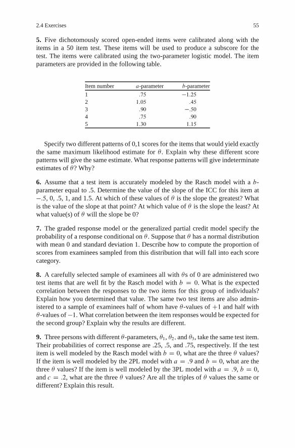
2.4 Exercises 55
5. Five dichotomously scored open-ended items were calibrated along with theitems in a 50 item test. These items will be used to produce a subscore for thetest. The items were calibrated using the two-parameter logistic model. The itemparameters are provided in the following table.
Item number a-parameter b-parameter
1 :75 �1:252 1:05 :45
3 :90 �:504 :75 :90
5 1:30 1:15
Specify two different patterns of 0,1 scores for the items that would yield exactlythe same maximum likelihood estimate for � . Explain why these different scorepatterns will give the same estimate. What response patterns will give indeterminateestimates of �? Why?
6. Assume that a test item is accurately modeled by the Rasch model with a b-parameter equal to .5. Determine the value of the slope of the ICC for this item at�:5, 0, .5, 1, and 1.5. At which of these values of � is the slope the greatest? Whatis the value of the slope at that point? At which value of � is the slope the least? Atwhat value(s) of � will the slope be 0?
7. The graded response model or the generalized partial credit model specify theprobability of a response conditional on � . Suppose that � has a normal distributionwith mean 0 and standard deviation 1. Describe how to compute the proportion ofscores from examinees sampled from this distribution that will fall into each scorecategory.
8. A carefully selected sample of examinees all with �s of 0 are administered twotest items that are well fit by the Rasch model with b D 0. What is the expectedcorrelation between the responses to the two items for this group of individuals?Explain how you determined that value. The same two test items are also admin-istered to a sample of examinees half of whom have �-values of C1 and half with�-values of �1. What correlation between the item responses would be expected forthe second group? Explain why the results are different.
9. Three persons with different �-parameters, �1, �2; and �3, take the same test item.Their probabilities of correct response are .25, .5, and .75, respectively. If the testitem is well modeled by the Rasch model with b D 0, what are the three � values?If the item is well modeled by the 2PL model with a D :9 and b D 0, what are thethree � values? If the item is well modeled by the 3PL model with a D :9, b D 0,and c D :2, what are the three � values? Are all the triples of � values the same ordifferent? Explain this result.

Chapter 3Historical Background for MultidimensionalItem Response Theory
Multidimensional item response theory (MIRT) is the result of the convergence ofideas from a number of areas in psychology, education, test development, psycho-metrics, and statistics. Two general themes underlie the influence of these ideas onthe development of MIRT. The first theme is that as our understanding of theseareas increases, it becomes clear that things are more complicated than originallythought. The second theme is that the complexity can be represented by modelsor theories, but these theories and models are idealizations of reality. Because theyare idealizations, they can likely be proven false if tested using a large number ofobservations. Nevertheless, the models can give useful approximations with manypractical applications.
It is common in the development of scientific theories to collect data about aphenomenon and then to develop an idealized model of the phenomenon that isconsistent with the data. The idealized model is usually presented as a mathemat-ical equation. An example of this approach to theory development is reported inAsimov (1972, p. 158). He describes Galileo in a church observing the swing oflamps hanging from the ceiling by long chains. These lamps were swinging likependulums, and Galileo is reported to have recorded the length of time it took tomake one full swing using his own pulse rate. From these observations, he devel-oped a mathematical formula that related the length of the chain to the length oftime for each swing (period) of a pendulum.
His model of the motion of pendulums was an idealization of reality in that it didnot take into account such factors as wind resistance and the elasticity of the chainused to support the lamps. He also did not have a fully developed theory of the swingof a pendulum in three-dimensional space. The model did not give an absolutelyprecise description of the observed phenomenon, the swing of the pendulum. Yet,despite the lack of precision, the mathematical model was, and still is, useful as adescription of the operational characteristics of pendulums.1
The same process of developing mathematical models to describe observed phe-nomenon was used by psychologists and statisticians such as Ebbinghaus (1885)
1 The approximation formula for the period of an ideal simple pendulum is p D 2�q
lengthg
, where
g is the acceleration due to gravity. The approximation holds when the angle of swing is small.
M.D. Reckase, Multidimensional Item Response Theory, Statistics for Socialand Behavioral Sciences, DOI 10.1007/978-0-387-89976-3 3,c� Springer Science+Business Media, LLC 2009
57

58 3 Historical Background for Multidimensional Item Response Theory
and Galton (1870). They observed various characteristics of individuals and de-veloped idealized models of the relationships among those characteristics. Theirmodels were far from precise representations of the observed phenomena, but inmany cases they yielded useful representations of the phenomena.
For each of these examples, the researchers did not expect the idealized modelsto describe every nuance of the observed phenomenon. Galileo probably did notexpect his mathematical equation to describe the period of swing for a pendulumwith a very light weight and a large cross-sectional area because air resistance wasnot included as an element in his model. The focus of his work was to provide amodel of the phenomenon for most practical applications of pendulums. Such mod-els are idealizations of the relationships present among the observed phenomenonin that erratic features have been smoothed out along with components that havevery minor effects on the relationships of interest. The same approach is followedwhen developing a mathematical model for the interactions between persons andtest items. The focus is on the major features of the relationship, rather than onthe components of the interaction that account for small perturbations. Even theseidealized models can often yield information that helps understand the principlesunderlying observed phenomenon, in this case, the responses to test items.
A convenient way to represent idealized models is through mathematical expres-sions. The observed phenomena are quantified and the hypothesized model is statedas a functional relationship between the observations and characteristics of the situ-ation. In general, these mathematical models take the following form:
y D f .x/; (3.1)
where y is the observation of interest and x is a vector of variables that describe theconditions under which the observation was made.
When using idealized models, it is not expected that y will be predicted withabsolute accuracy by the application of the function to the elements of the vector x.It is only expected that a good approximation for y will be determined. Nor is themathematical model thought to be “true” in an absolute sense. It is expected that asmore observations are made, a more refined model will be developed. At best, it isexpected that the model will be useful for describing the relationship between obser-vations and the conditions of observation, or provide insights into the relationshipsamong observed variables.
MIRT is a model or theory that is an idealization of reality. It gives only anapproximation to the relationship between persons’ capabilities and the responsesto test items. The theory states that a particular mathematical expression can give areasonably accurate representation of the relationship between persons’ locations ina multidimensional space and the probabilities of their responses to a test item. Atthis stage in the development of MIRT, the mathematical expressions used to modelthe relationships are fairly simple. As more is learned about people and test items, itis likely that more complex mathematical expressions will be used that more closelyrepresent the relationships between persons’ abilities and the characteristics of testitems. Despite the fact that MIRT models are a simplification of reality, they are still

3 Historical Background for Multidimensional Item Response Theory 59
useful. Later chapters of this book will provide examples of the application of MIRTmethodologies to practical testing problems.
In some cases, models for phenomenon do not work directly with the observationof interest. For example, when modeling the relationship between temperature andthe pressure on a fixed amount of gas, the observation that is used is not the rate ofmolecular motion or the energy level of the gas. Rather, it is the height of the surfaceof a liquid in a glass tube such as a mercury thermometer, or the expansion of metalsin a bimetal thermometer. The thermometers give a representation of temperature,but the expansion of liquid or metal is not really temperature or heat. Further, theheight of the surface of the liquid or expansion of metal is measured on an arbitrarynumerical scale such as the Celsius temperature scale.
Work in educational and psychological measurement has followed the samedevelopmental path as other areas of science. Many idealized models have beenhypothesized for the observed phenomenon, usually responses to test items, andcharacteristics of persons (see van der Linden and Hambleton 1997, for many ex-amples). The characteristics of the persons are usually measures of hypotheticalconstructs. The models often relate the probability of a response to person charac-teristics rather than to the response itself. This is similar to using the height of liquidto represent temperature rather than measuring the energy in molecular movement.When modeling item/person interactions, working with probabilities allows sim-pler mathematical models and acknowledges the uncertainty in the hypothesizedrelationships. Because the models relate probabilities of test item responses to thecharacteristics of persons, they are called “item response theory” (IRT) models.
The later chapters of this book present a collection of mathematical models thatare useful for describing the interactions between persons and test items. Thesemodels differ from many of the other IRT models in that they posit that multi-ple hypothetical constructs influence the performance on test items instead of onlyone hypothetical construct. Therefore, they are labeled MIRT models (Reckaseet al. 1988). As with other IRT models, the actual observations that are the focus ofthe models are the responses to test items. In most cases, the models are for scoredtest items rather than the actual response. The most commonly used models are foritems scored using two categories – correct and incorrect – although MIRT modelsfor items with more than two score categories also exist (see Chap. 4 for some ex-amples). MIRT models probabilities of responses rather than the actual responses.The basic form of the models considered here is
P.U D uj™/ D f .u; ™;”/; (3.2)
where U is the score on the test item for a particular person, u represents the valueof the assigned score from among the possible scores to the test item, ™ is a vectorof parameters describing the location of the person in the multidimensional space,and ” is a vector of parameters describing the characteristics of the test item.
The item score, u, is included on the right side of the expression because the formof the prediction equation may change depending on the score a person receives forhis or her response to the test item. Of course, if the score on the item rather than

60 3 Historical Background for Multidimensional Item Response Theory
the probability of the score were being predicted, the presence of the score on bothsides of the equal sign would form a trivial tautology. Because the probability isbeing predicted, the presence of u on the right side of the expression is a convenientway to select the desired prediction equation.
None of the models presented here is believed to be a true representation of thepsychological processes that underlie the interaction between a person and a testitem. In all cases, it is expected that with the collection of enough data, all of themodels can be shown to be false. However, one purpose of this book is to sum-marize the research that shows when these models provide useful idealizations ofthe relationship between hypothetical constructs and observed phenomena – latenttraits and responses to test items. The criteria for usefulness are whether the modelsyield reasonably accurate predictions of actual observations or if they help reach anunderstanding of the interrelationships among variables of interest.
The remaining sections of this chapter will provide a historical context that un-derlies the development of the MIRT models. Both the psychological context thatled to thinking about many dimensions of variation in the cognitive skills for peo-ple and the psychometric context that led to the development of multidimensionalmodeling procedures are presented. Although unidimensional IRT can legitimatelybe thought of as part of the psychometric context for MIRT, it is not included in thischapter. Rather, Chap. 2 gave a summary of the unidimensional IRT concepts thatare helpful for understanding the development of MIRT concepts.
3.1 Psychological and Educational Context for MIRT
As with other areas of science and technology, psychological and educational testingfirst developed relatively simple theories and testing methods to obtain the quanti-tative variables needed to further develop those theories. Early models of atomsconsidered them as solid balls. Current models of the atom have numerous smallparticles and energy fields within the atom.
MIRT methodology developed in response to a realization that psychologi-cal and educational processes are very complex. This complexity became evidentthrough the findings from many years of research. For example, in the 1950s, psy-chological research on memory focused on “immediate memory” and “chunking”(Deese 1958). The rule of thumb that individuals could remember about seven thingsafter a single presentation was being investigated to determine what constitutes a“thing.” In contrast, the 1996 volume of the Annual Review of Psychology containsa 25 page summary on the topic of memory (Healy and McNamara 1996) that in-cludes concepts such as primary and secondary memory stores, associative memory,permastore, and precategorical acoustic store. Current memory models are muchmore complex than those in the past, and they are likely to be more complex inthe future.
The study of variation in the cognitive abilities of people shows a similar pat-tern of increase in complexity as greater understanding is attained. Vernon (1950,

3.2 Test Development Context for MIRT 61
p. 49) stated that “no intellectual faculties beyond g [general ability] and v [verbalability] are yet established as having much educational or vocational importance.”In contrast to this relatively simple conception of abilities, Carroll (1993, p. 147)identifies 15 factors related to language ability. Many of those factors have many“token” factors. For example, verbal or printed language comprehension (V in Car-roll’s notation) has 150 token factors. Clearly, the psychological conceptualizationof cognitive abilities has become much more complex as the result of continuingresearch. Other achievement and aptitude areas have equally complex structures.Further, research in cognitive sciences (e.g., Frederikson et al. 1990) shows thatmany skills are needed to respond correctly to single test items.
There is a similar pattern in the development of educational concepts. The earlyconception of reading comprehension was “How much did the child get out of whathe read?” (Burgess 1921, p. 18). Reading skill was assessed by having students reada story and write as much as they could remember (Kallon 1916). The currentconception of reading comprehension is much more complex. The 2005 NationalAssessment of Educational Progress (NAEP) describes fourth grade reading in thisway (Perie et al. 2005).
“reading . . . includes developing a general understanding of written text, thinking abouttexts, and using texts for different purposes. In addition [the Governing Board] views read-ing as an interactive and dynamic process involving the reader, the text, and the context ofthe reading experience.” (p. 24)
NAEP assesses reading skill and knowledge using a complex set of item types in-cluding multiple-choice, open-ended, and extended response items. The implicationis that the different item types are needed to assess the breadth of skills that encom-pass “reading.” The reading passages on NAEP also vary in a number of differentways including the type of content, the structure of the writing (i.e., narrative, ar-gumentative, etc.), and the length. The conceptual understanding of reading haschanged in dramatic ways since 1921. The trend has been to consider it a morecomplex process requiring multiple skills.
3.2 Test Development Context for MIRT
The process for developing tests has become more complicated over the years. Earlytests consisted of sets of tasks that were selected in unspecified ways.Whipple (1910,p. 460) describes the procedures for administering and scoring many early tests. Oneexample is an assessment of size of a student’s vocabulary. Students were given alist of 100 words and they were asked to write a definition for each. The results werescored by counting the number of correct definitions. The results were converted toa proportion correct and that number was multiplied by 28,000 to give an estimateof the size of the student’s vocabulary. The number 28,000 was used because itwas assumed to be the maximum size for a person’s vocabulary. No informationwas given about how the words were selected, but they included some interestingchoices like “amaranth” and “eschalot.”

62 3 Historical Background for Multidimensional Item Response Theory
Current test development processes are much more complex, not only becauseof more elaborate conceptions of the constructs to be measured, but also becauseof the level of detail provided in test specifications. Millman and Greene (1989)provide a thorough description of the test development process. Their 32 page chap-ter includes substantial discussions of the development of test specifications andthe match of item types to the specific content. More recent work demonstrateseven more dramatically the complexity of current test development procedures. vander Linden (2005) indicates that computerized test assembly procedures sometimeshave hundreds of constraints that must be met when selecting items for a test.
There is a certain irony in the evolution of the scoring of tests. Thorndike (1904)found it obvious that different test items required different amounts of skill andknowledge and they should be scored to reflect their complexity. Yet, the majortests that were developed in the early 1900s treated items as equal units. The ArmyAlpha Tests (Yoakum and Yerkes 1920) clearly indicated that each item is scoredeither right or wrong and the score is the number right. The tests based on the workof Binet and Simon (1913) used very complex items, but Stern (1914) indicates thatresponding correctly to five tests (his label for items) increased the mental age by1 year. The advice from McCall (1922, pp. 249–250) was to produce a test that didnot have zero scores or perfect scores and that had at least seven reporting categories.He further advised that there be at least 13 reporting categories if correlations weregoing to be computed. Although unstated, the implication was that the score on atest was the sum of the points allocated for each item. Different test items could havedifferent numbers of allocated points. By 1950, little had changed about the scoringof tests. Gulliksen (1950) does not raise the issue of what the test is measuring butonly assumes that “the numerical score is based on a count, one or more pointsfor each correct answer and zero for each incorrect answer” (p. 4). Everything inhis book on test theory is built on the characteristics of that type of score. He alsolaments that for most item analysis methods “no theory is presented showing therelationship between the validity or reliability of the total test and the method ofitem analysis” (p. 363).
With the implementation of item response theory methods, scoring has becomemore complex. Methods based on the two and three-parameter logistic models (seeChap. 2) give items different weights depending on the discriminating power ofthe items. The use of the three-parameter logistic model also reduces the relativeimpact of correct responses to that of incorrect responses on the estimates of profi-ciency because of the possibility that they may have been obtained by chance. Theprocess of scoring tests using these models is called “pattern scoring” because dif-ferent patterns of responses to the set of items on a test give different scores, evenwhen the number of correct responses is the same. The book edited by Thissen andWainer (2001) provides an extensive discussion of test scoring methodology.
The trend in test design and development, and test scoring is to consider the testitem as the basic component of test design rather than the test as a whole. This isthe basic difference between item response theory and true score theory. The for-mer focuses on characteristics of test items and how they combine to make tests.The later assumes that a test has been constructed and focuses on the characteristics

3.3 Psychometric Antecedents of MIRT 63
of test scores. MIRT continues the trend toward treating the test item as the fun-damental unit of test construction. It extends the work from unidimensional IRT togive a more thorough description of the characteristics of test items and how theinformation from test items combines to provide a description of the characteristicsof persons.
3.3 Psychometric Antecedents of MIRT
Depending on a psychometrician’s background, MIRT may be considered as ei-ther a special case of multivariate statistical analysis, especially factor analysis orstructural equation modeling, or as an extension of unidimensional IRT. These twoconceptualizations of MIRT color the way that the methodology is applied and theway that the results of MIRT analyses are interpreted. Because of the strong con-nection of MIRT to both of these psychometric traditions, it is helpful to review theprecursors to MIRT from both of these areas. The next sections of this chapter willsummarize both perspectives and highlight the differences.
3.3.1 Factor Analysis
A review of the mathematical procedures used for factor analysis and MIRT willreveal that there are numerous similarities in the statistical underpinnings of themethods. Both methods define hypothetical scales that can be used to reproducecertain features of the data that are the focus of the analysis. For both of the pro-cedures, the scales have arbitrary zero points (origins) and units of measurement.They also specify systems of coordinate axes that can be rotated to emphasize cer-tain characteristics of the data. MIRT differs from most implementations of factoranalysis in that the varying characteristics of the input variables (the items), such asdifficulty level and discrimination, are considered to be of importance and worthyof study. Factor analysis implementations typically consider the differences in thecharacteristics of input variables as nuisances to be removed through transforma-tions that standardize the variables to have common means and standard deviations.Because of the lack of interest in the characteristics of the variables in the analy-sis, most factor analysis texts begin with the analysis of a correlation matrix, a datasource that ignores differences in means, and standard deviations of the variables.For example, Harman’s (1976) classic work on factor analysis describes the purposeof the analysis as follows:
“The principal concern of factor analysis is the resolution of a set of variables linearly interms of (usually) a small number of categories or ‘factors.’ This resolution can be accom-plished by the analysis of the correlations among the variables.” (p. 4)
Even when factor analysis is applied to item scores, usually 0 or 1, the charac-teristics of the variables, such as difficulty and discrimination, are not considered.

64 3 Historical Background for Multidimensional Item Response Theory
In fact, a major motivation for some of the variations in factor analysis proceduresdescribed later is dealing with difficulty factors. These were factors that resultedfrom variation in difficulty of dichotomously scored test items. The difficulty fac-tors were a consequence of the relationship between proportion correct for the testitems and the magnitude of the Pearson product-moment correlation between testitems. Only test items with proportions correct of .5 can have correlations of 1.Similarly, tetrachoric correlations have more unstable estimates when the cells of atwo-by-two table of scores on test items have near zero frequencies.
Another issue related to the characteristics of test items is the possibility thata person might guess the correct answer. Factor analysis does not usually haveany way to adjust for the possibility of guessing on multiple-choice test items.Rather, guessing is considered as another nuisance feature of the data that shouldbe removed through a correction to the process of computing the correlations(Carroll 1945).
As with any scientific endeavor, experts in a field do not always agree on an ap-proach or basic philosophy. This is also true for those developing the factor analysismethodology. Several researchers chose to address the problem of how to identifyhypothetical variables that would allow the reproduction of the relationships in thedata from a slightly different perspective than most others. The contributions of fiveresearchers are described here because their work contributed to the foundations forMIRT. These individuals should be considered as representatives of a set of contrib-utors rather than the sole proponents of a point of view. Many others, no doubt, hadsimilar perspectives on factor analysis. These five were selected because they werethe most visible in the literature and were most active in advancing their perspectiveover a period of years.
Horst
Paul Horst was one of the early contributors to the field of factor analysis who fore-shadowed the development of MIRT. The major distinction between his approachand that of other factor analysts is that he advocated developing factor models thatcould reproduce the full data matrix rather than the correlation matrix. This perspec-tive is described in detail in his book Factor Analysis of Data Matrices (Horst 1965).His perspective is summarized as follows.
“It should be observed at the outset that most treatments of factor analysis do not, how-ever, begin with a consideration of the x matrix [the matrix of observed scores] as such andthe determination of the u matrix [the matrix of true scores]. These treatments usually beginwith the correlation matrices derived from the x matrix. This approach has led to much mis-understanding because the analyses applied to the correlation matrix sometimes imply thatthere is more information in the correlation matrix than in the data matrix x. This can neverbe the case. For this reason, as well as others, it is much better to focus attention first on thedata matrix, as such, in considering the problems and techniques of factor analysis.” (p. 96)

3.3 Psychometric Antecedents of MIRT 65
Because Horst worked from the observed score matrix, he had to confront issuesrelated to the characteristics of the variables. His book contains extended discus-sions of the issues of origin and unit of measurement and the effects of scalingtransformations on factor analysis results. More importantly for this discussion ofMIRT, he argued against trying to standardize the variables when factor analyzing abinary data matrix. Rather, he suggested partialing out the effects of variation in itemdifficulty, or as he called it, the “dispersion of item preferences.” This procedure iscalled “partialing out the simplex” and it is conceptually similar to estimating thedifficulty parameters of the items and using the estimates to model the data.
Although there are many similarities between Horst’s work and current concep-tions of MIRT, he did not quite get to the point of developing MIRT models. He wasattempting to recover the actual data rather than the probability of a response andhe did not consider factor loadings as item parameters. The emphasis of the analy-sis was on the factors – the coordinate system, rather than item characteristics andperson locations.
Christoffersson and Muthen
The methodologies developed by Christoffersson (1975) and Muthen (1978) areconceptually closer to current thinking about MIRT than those presented byHorst (1965). They produced probabilistic models for the relationship betweenitem responses and vectors of person parameters. Both used a normal ogive modelto obtain estimates of threshold parameters for items. The threshold parametersare the normal deviate values that specified the area beneath the normal curveequal to the proportion of incorrect responses to the items. These parameters areessentially the same as the item difficulty parameters for a MIRT model.
Christoffersson (1975) states: “we see that the model Œp D � C "2 expressesthe observed proportions p in terms of the threshold levels zi ; i D 1; 2; : : : ; n, theloadings A, the factor correlations R and a random component ".” � is given by thefollowing equation involving the integral of the normal density
�i D P.ui D 1/ D1Z
zi
1p2�
e� t2
2 dt ; (3.3)
where ui is the item score on Item i , and zi is the threshold parameter for Item i .Christoffersson’s formulation of the relationship between item responses and
hypothetical latent variables uses factor loadings and threshold estimates as item
2 The original presentations of factor analytic and IRT models used a wide variety of symbols torepresent the parameters of the models. To make comparisons of the models easier, the symbolshave been changed to a common set. This means that the symbols used here may not match thosein the original article.

66 3 Historical Background for Multidimensional Item Response Theory
parameters. These parameters are very similar to those used to describe the char-acteristics of test items in MIRT. The major differences between Christoffersson’srepresentation and MIRT are that he focused on modeling continuous item scoresunderlying the dichotomous observed scores rather than the locations of individ-uals in a multidimensional space. Further, the probabilities of correct response inthe model are not conditional on the location of a person in the multidimensionalspace as they are in current MIRT models (see Chap. 4). Instead, the focus is on theprobability of correct responses for the entire population of examinees.
Muthen (1978) expanded on Christofferson’s work. He developed a model thatincluded both the probability of correct response for a single item for the examineepopulation and the probability that the examinee population would give correct re-sponses to pairs of items. These probabilities were included in a single vector, p,with the first n elements containing the probabilities for single items and the nextn.n � 1/=2 elements containing the probabilities for correct responses to each pos-sible pair of items. Muthen’s model is
p D f .�/C e; (3.4)
where � is partitioned into two parts, (�01, �0
2), �01 is an n-dimensional vector of
thresholds, �02 is a n.n � 1/=2 element vector of population tetrachoric correla-
tions between items, and e is a matrix of errors in predicting the probabilities.The function, f ./, relates the probabilities using the univariate or bivariate nor-mal density function to the descriptive characteristics of the test items. As in thework of Christofferson, the population probabilities of correct responses were mod-eled rather than the conditional probabilities for persons with specified vectors oflocation parameters.
Both Christofferson and Muthen came very close to presenting the current for-mulation for MIRT. However, neither of their models was based on the conditionalprobability of correct response to each item as a function of a person’s location ina multidimensional space. Rather, they modeled the probability of correct responsefor the full population of examinees.
McDonald
The nonlinear factor analysis methodology proposed by McDonald (1967) is prob-ably the presentation of factor analysis that is most similar to the current conceptionof MIRT. McDonald addressed the problem of factor analyzing variables that havevalues of 0 or 1. He indicated that concerns about the appearance of difficulty factorswhen dichotomous data are analyzed could be overcome if the relationship betweenthe observed data and the hypothetical factors is allowed to be nonlinear. McDonaldalso clearly specified the important concept of local independence as the basis forthe analysis of test items.

3.3 Psychometric Antecedents of MIRT 67
The general form of the principle of local independence is
h.xj™/nY
iD1hi .xi j™/; (3.5)
where x is the vector of observed responses, ™ is the vector of latent“characterizations,”and h.xj™/ is the conditional density of the observed response vector given thelatent “characterizations.” In current terminology, McDonald’s “characterizations”are abilities or proficiencies needed to respond correctly to the test item.
McDonald also represented the basic form of the relationship between the prob-ability of correct response to an item and the coordinates of the location of personsin the ability space as the regression of the item score on ability. He also noted thatthe connection between the regression function and the conditional probability ofcorrect response is
Pi.™/ � E.ui j™/; (3.6)
where Pi .™/ is the probability of correct response to Item i .The difference between McDonald’s (1967) formulation and current MIRT repre-
sentations is that he used a polynomial model to represent the interaction of personswith a test item rather than the logistic or normal ogive models. The polynomialmodel was used as an approximation to the normal ogive model. Also, he did notprovide any interpretation for the item parameters. The focus was on estimating thefactors rather than understanding the characteristics of the items or the interactionsbetween persons and items. More recent work by McDonald (1985, 1999) makesthe relationship between factor analysis and MIRT very clear. In fact, McDonaldconsiders factor analysis as a special case of latent trait theory. “The view takenhere is that common factor analysis is really a special case of latent trait theory,based on the principle of local independence, but one in which for convenienceonly the weak zero-partial-correlation version of the principle is typically tested”(McDonald 1985).
Bock and Aitkin
The methodology presented in Bock and Aitken (1981) provided the convergenceof ideas from IRT and factor analysis that resulted in MIRT. They defined a normalogive model for a multidimensional ability space that included characterizations oftest items using both factor analytic and IRT representations. Their model is given by
P.xij D 1j™j / D 1p2�
1Z
�zi .™j /
e� t2
2 dt; (3.7)

68 3 Historical Background for Multidimensional Item Response Theory
where zi .™j / D di C ai™j0; ai is the 1�m vector of item discrimination parameters
for Item i , di is a scalar parameter related to the difficulty of Item i , and ™j is a1 � m vector of proficiencies for Person j . The parameters of the model have thesame meaning and interpretation as the current MIRT parameterization.
Bock and Aitken demonstrated the use of this model through an analysis of testitems from the Law School Admissions Test (LSAT) Section 7. The item difficultyand discrimination parameters were estimated, but they were labeled as slopes andintercepts. The only distinction between the Bock and Aitken (1981) analysis anda full MIRT conceptualization was the interpretation of the item parameters as de-scriptive measures that were useful for describing the interactions of persons andtest items. The item parameters were still used in a factor analytic sense as a meansto help label the factors.
Although the model presented in Bock and Aitken (1981) is essentially a MIRTmodel, its major use was as a factor analytic model as shown in Bock, Gibbons, andMuraki (1988). The emphasis was still on defining factors rather than investigatingthe interactions between persons and items.
3.3.2 Item Response Theory
The focus of item response theory (IRT) is quite different than that of factor analysis.Rather than trying to determine the minimum number of factors that can reproducethe data in a matrix of item responses, IRT analyses try to model the relation-ship between persons’ characteristics and the features of test items. Lord (1980)expressed the goal of IRT this way.
“We need to describe the items by item parameters and the examinees by examinee param-eters in such a way that we can predict probabilistically the response of any examinee toany item, even if similar examinees have never taken similar items before.”
Early work in IRT was based on the assumption that the parameter that describesthe examinees varies on only one dimension (Lord and Novick 1968; Rasch 1960),but it quickly became apparent that the unidimensionality assumption was oftenviolated. Work still continues on determining the consequences of violating the uni-dimensionality assumption (e.g., Camilli et al. 1995; Kirisci et al. 2001; Wang andWilson 2005).
The remainder of this section presents some early attempts to consider multidi-mensionality in IRT. The final section of this chapter provides a direct comparisonof the IRT perspective with the factor analysis perspective.
Rasch
The earliest published work of Rasch (1960) dealt only with unidimensional IRTmodels. However, in 1962 he presented a generalization of his initial models that

3.3 Psychometric Antecedents of MIRT 69
included the possibility that the ability of the examinee could be represented bya vector or proficiencies rather than by a scalar (Rasch 1962). The general Raschmodel is given by
P.uijj™j;˜i/ D 1
�.�j;˜i/ef .uij/
0™jCg.uij/0˜iC™j
0h.uij/˜iC`.uij/; (3.8)
where f, g, h, and ` are scoring functions for the item. That is, the functions indicatehow the items are scored for each proficiency dimension, each dimension of sensi-tivity of the items, and the interaction of the two types of dimensions. The function“f ” indicates the score that corresponds to each item response for each dimensionin ™. For the unidimensional Rasch model, only two scores are given to the item –1 for a correct response and 0 for an incorrect response. The function “g” indicatesthe weights given to the item parameters for each dimension for each item. For theunidimensional model, these are 1 for a correct response and 0 for an incorrect re-sponse. The function “h” gives weights for the interaction between person and itemparameters. The value of this function is 0 for all responses for the unidimensionalmodel. The function “`” allows for a fixed constant term for the item. This functionis set to 0 for all responses for the unidimensional model. All of these functions arefixed in advance of the application of the model rather than estimated from the data.Fixing these functions maintains the critical property of the Rasch model of havingobservable sufficient statistics for the person and item parameters. The function “�”generates a normalizing constant that is the sum of all of the possible exponentialterms. Dividing by this function causes the probabilities for the possible responsesto sum to 1.0.
The different functions in the general Rasch model have been used by Fischerand Molenaar (1995) to develop complex linear logistic model. Reckase (1972) andKelderman (1994) used the scoring functions to apply the model to what are nowcalled “testlets” or for items with more than two score categories. Glas (1992) usedthe scoring functions to indicate the content dimensions measured by the items.More recent work, such as Rijmen and De Boeck (2005), also used this approach.Glas and Vos (2000) have used this model in an adaptive testing context. This modelis described in more detail in Chap. 4.
Lord and Novick
The basic requirements for a MIRT model were presented in Chap. 16 of Lord andNovick (1968), although a complete MIRT model was not presented. The chap-ter includes definitions of a complete latent space and the assumption of localindependence.
Local independence means that within any group of examinees all characterized by the samevalues �1; �2; : : : ; �k , the (conditional) distribution of the item scores are all independent ofeach other. (p. 361)
The vector ™ defines the complete latent space.

70 3 Historical Background for Multidimensional Item Response Theory
Lord and Novick (1968) also presented the relationship between the unidimen-sional normal ogive IRT model and the common factor model. It is notable, however,that the major portion of Chap. 16 is a discussion of the meaning of the item param-eters and their use for solving practical testing problems. The focus is not on themeaning of factors resulting from the common factor model.
Samejima
Samejima (1974) gave another early presentation of a proposed MIRT model. Al-though most IRT models have been developed for items that are scored eitherdichotomously or polytomously, it is also possible to have items with scores on acontinuous scale. Samejima generalized her continuous response model to the casewith a ™ - vector. The model is given by
Pzi .™j/ D 1p2�
ai0.™j�bi /Z
�1e� t2
2 dt; (3.9)
where zi is the continuous response to Item i; P is the probability of obtaining ascore of z or better on Item i;bi is a vector of difficulty parameters, with otherparameters as previously defined.
Although the Samejima (1974) model is one of the first formal presentationsof a MIRT model, it has not been widely used. Bejar (1977) provided the onlyapplication of the model that could be found. The lack of use is probably related tothe rarity of applications for continuous response items.
3.3.3 Comparison of the Factor Analytic and MIRT Approaches
Factor analysis and MIRT have virtually identical statistical formulations whenthey are applied to matrices of item responses. This can be noted from a com-parison of the models presented by Bock and Aitken (1981), Samejima (1974),and McDonald (1967). In fact, the software for the full information factor analysismethodology presented by Bock et al. (1988) can be used for either factor analysisor MIRT.
If the statistical procedures are virtually identical, what is the difference in thetwo types of methodology? First, factor analysis is thought of as a data reduc-tion technique. The goal is usually to find the smallest number of factors thatreproduces the observed correlation matrix. MIRT is a technique for modelingthe interaction between persons and test items. Reckase and Hirsch (1991) haveshown that using too few dimensions might degrade the modeling of the item/person

3.4 Early MIRT Developments 71
interactions, but using too many dimensions does not cause serious problems. Thus,MIRT may be a better analysis tool when it is not thought of as a data reduction tech-nique. It is a method for modeling the meaningful contributors to the interactions ofpeople with test items.
Second, factor analysis typically ignores the characteristics of the input variableswhile MIRT focuses on them. Analyzing the correlation matrix implies that differ-ences in means and variances of variables is of little or no consequence. On theone hand, newer versions of factor analysis, such as structural equation modeling,do consider means, variances, and covariances, but not for the purpose of getting abetter understanding of the input variables. MIRT, on the other hand, focuses on thedifferences in means and variances of the item scores because they are directly re-lated to important characteristics of test items such as difficulty and discrimination.These item characteristics are actively used in MIRT applications.
Finally, MIRT analyses actively work to find solutions that use the same latentspace across tests and samples. The goal is to keep a common coordinate systemfor all analyses so that the items will have parameter estimates on common metrics.Having item parameters on a common metric support their storage in an item bankfor use in test forms construction and computerized adaptive testing. Factor analysisprocedures have developed some procedures for putting the solutions into commoncoordinate systems, but those methods are not widely used. Instead, factor analysismethods now emphasize confirmatory methods and structural equation modeling.The methods developed for factor analysis like Procrustes rotations are now beingused to place MIRT solutions onto common scales. Such methods are an extensionof unidimensional IRT methods for test equating and linking of calibrations. Devel-oping methods for linking calibrations from different tests and examinee samples isa major part of the research on MIRT. These methods will be described in detail inChap. 9 of this book.
3.4 Early MIRT Developments
In the late 1970s and early 1980s, a number of researchers were actively workingto develop practical MIRT models. In addition to the work by Reckase (1972) onthe multidimensional Rasch model (see (3.8)), Mulaik (1972), Sympson (1978),and Whitely (1980a,b) suggested multidimensional models for the item/personinteraction.
The Mulaik (1972) model is given by
P.uijj™j;˜i/ D
mP
kD1e.�jk�ik/uij
1CmP
kD1e.�jk�ik/uij
; (3.10)
where the symbols have the meaning defined previously and uij D 0 or 1. Thismodel has an interesting property. For fixed values of the exponent, the probability
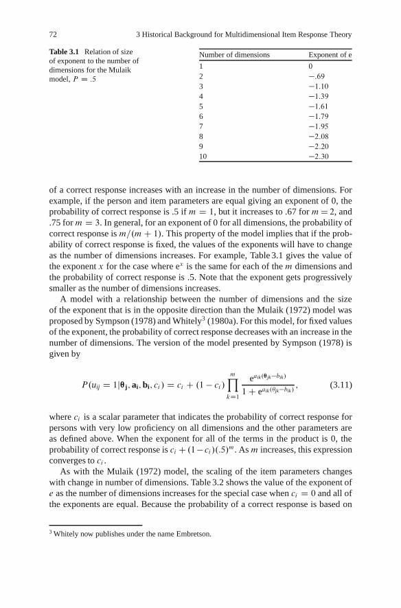
72 3 Historical Background for Multidimensional Item Response Theory
Table 3.1 Relation of sizeof exponent to the number ofdimensions for the Mulaikmodel, P D :5
Number of dimensions Exponent of e
1 02 �:693 �1:104 �1:395 �1:616 �1:797 �1:958 �2:089 �2:2010 �2:30
of a correct response increases with an increase in the number of dimensions. Forexample, if the person and item parameters are equal giving an exponent of 0, theprobability of correct response is .5 if m D 1, but it increases to .67 for mD 2, and.75 form D 3. In general, for an exponent of 0 for all dimensions, the probability ofcorrect response is m=.mC 1/. This property of the model implies that if the prob-ability of correct response is fixed, the values of the exponents will have to changeas the number of dimensions increases. For example, Table 3.1 gives the value ofthe exponent x for the case where ex is the same for each of the m dimensions andthe probability of correct response is .5. Note that the exponent gets progressivelysmaller as the number of dimensions increases.
A model with a relationship between the number of dimensions and the sizeof the exponent that is in the opposite direction than the Mulaik (1972) model wasproposed by Sympson (1978) and Whitely3 (1980a). For this model, for fixed valuesof the exponent, the probability of correct response decreases with an increase in thenumber of dimensions. The version of the model presented by Sympson (1978) isgiven by
P.uij D 1j™j; ai;bi; ci / D ci C .1 � ci /
mY
kD1
eaik.™jk�bik/
1C eaik.�jk�bik/; (3.11)
where ci is a scalar parameter that indicates the probability of correct response forpersons with very low proficiency on all dimensions and the other parameters areas defined above. When the exponent for all of the terms in the product is 0, theprobability of correct response is ci C .1� ci /.:5/m. Asm increases, this expressionconverges to ci .
As with the Mulaik (1972) model, the scaling of the item parameters changeswith change in number of dimensions. Table 3.2 shows the value of the exponent ofe as the number of dimensions increases for the special case when ci D 0 and all ofthe exponents are equal. Because the probability of a correct response is based on
3 Whitely now publishes under the name Embretson.

3.4 Early MIRT Developments 73
Table 3.2 Relation of sizeof exponent to the number ofdimensions for the Sympsonmodel, P D :5
Number of dimensions Exponent of e
1 02 .93 1.34 1.75 1.96 2.17 2.38 2.49 2.510 2.6
the product of m terms and the terms are all less than 1.0, the terms must increasein value with increase in m to yield the same probability of correct response.
Reckase (1972) investigated the use of the general Rasch model given in (3.8) anddetermined that it was not possible to model multidimensional data from dichoto-mously scored items with that model unless the scoring functions were defined inadvance of the estimation of the parameters. Instead, he grouped together sets ofitems to form what are now called testlets to allow the estimation of the scoringfunctions. Recent work (e.g., Wilson and Adams 1995) using the model in (3.8) hasbeen based on fixing the scoring functions prior to estimating the model parameters.The scoring function is defined based on characteristics of the items such as relationto a common stimulus or having a common content framework.
McKinley and Reckase (1982) further considered variations on the model givenin (3.8) and determined that the current multivariate form of the linear logistic modelwas the most useful and practical for exploratory analyses of data from tests com-posed of dichotomous items. The model as they presented it is given by
P.uij D 1j™j; ai; di / D e
mP
kD1
aik�jkCdi
1C e
mP
kD1
aik�jkCdi; (3.12)
where the symbols have the same meaning as in previous definitions. This modelwas labeled as a multivariate extension of the two-parameter logistic model becauseit has two item parameters – a vector of a-parameters (discrimination parameters)and a d�parameter. The two-parameter logistic model is described in the Chap. 2.
The model in (3.12) does not change scales for the parameters with the numberof dimensions like those presented in (3.10) and (3.11) because the combination ofdimensions is in the exponent of e. As long as the sum of the terms in the exponenthas the same value, the probability of correct response stays the same. The numberof dimensions does not have a direct effect on the probability. For example, if theexponent sums to 0, the probability of correct response is .5. Adding more terms tothe sum in the exponent (i.e., adding more dimensions) without changing the valueof the sum will not change the probability of a correct response.

74 3 Historical Background for Multidimensional Item Response Theory
3.5 Developing Applications of MIRT
The applications of MIRT have evolved since the early developments of the models.Initial applications focused on investigating the structure of relationships amongitem responses (e.g., Bock and Aitken 1981; McDonald 1967). The applicationshave evolved in a number of different ways since that time. A brief summary ofsome of the applications of MIRT is given here. The details of methodology forthose applications are given in Chaps. 8–10. MIRT is a very active area of current re-search. Additional applications will no doubt appear in the research literature beforethe publication of this book. The journals Psychometrika and Applied PsychologicalMeasurement often publish research articles on MIRT. Other journals that publishresearch on educational and psychological measurement are likely to have occa-sional articles on applications of the methodology.
Following the initial developments that followed the factor analytic tradition,Reckase (1985) and Reckase and McKinley (1991) developed ways of describingthe results of a MIRT analysis that were more consistent with IRT conceptualiza-tions. They developed graphic ways of describing the combinations of dimensionsthat are assessed by a test item, and ways of describing the difficulty and discrimi-nation of items in a multidimensional context. These methods will be described indetail in Chap. 5 of this book.
The focus of MIRT analysis on the interaction of the characteristics of test itemsand those of examinees has naturally led to fine grained studies of the skills andabilities need to respond correctly to test items, and to determine the dimensions ofsensitivity for test items. Miller and Hirsch (1992), for example, have analyzed anumber of different tests using a combination of MIRT and cluster analysis to iden-tify sets of test items that measure the same combination of skill and knowledgedimensions. The particular dimensions of sensitivity of the items were determinedthrough detailed content analysis of the item text for the identified clusters of items.In some cases, the clusters of items accounted for less variance than would typi-cally be considered meaningful through traditional factor analysis. Yet, the clusterswere replicable over multiple samples of examinees and different tests. In somecases, these small clusters of items that accounted for small proportions of variancein a full sample were very important for identifying specific subsamples with spe-cial characteristics such as scholarship candidates. Since that early work, there havebeen numerous studies on the detailed structure of item response data. This area ofresearch shows the importance of a thorough understanding of the ways that testsfunction.
MIRT analysis clearly shows that test items can be sensitive to examinee differ-ences on multiple dimensions. If these differences are on dimensions that are goalsof the assessment, the test is said to yield results that are valid indicators of the targetdimensions. But items may be sensitive to other dimensions that are not the goalsof the assessment. If subgroups of the examinee population differ on the dimensionsthat are other than the goal dimensions, sometimes called nuisance dimensions, thenthe reported results may include test bias. MIRT analyses can help identify groupdifferences and item sensitivities that contribute to test and item bias. The results

3.6 Influence of MIRT on the Concept of a Test 75
of MIRT analyses can help clarify the reasons for large differential item function-ing (DIF) statistics. Ackerman (1992) provided a clear representation of DIF usingMIRT models.
MIRT procedures have also been used to support the selection of items for a testso that the assumptions of unidimensional IRT will be met even when the itemsclearly require multiple skills and knowledge to determine the correct answer. Thisuse of MIRT makes it possible to support the use of unidimensional IRT for awide range of testing applications, such as measuring achievement in school sub-jects. Reckase et al. (1988) demonstrated the process of item selection that meetsunidimensional IRT requirements. These results show that the unidimensionalityassumption is not as restrictive as was once thought.
Another example of MIRT applications is the problem of putting calibrationsof different sets of items into the same multidimensional coordinate system. Thisprocess is typically called linking of calibrations and it is closely related to theequating of test forms. Davey and Oshima (1994) and others have addressed thisproblem. Their work shows that it is possible to put the parameter estimates frommultiple calibrations into the same coordinate system. This allows performance ondifferent sets of items to be reported as profiles on multiple dimensions that areon the same scales. It is also possible to develop large pools of calibrated items thatcan be used for computerized adaptive testing and the construction of test forms thatare multidimensionally parallel.
These and other applications are described in later chapters of this book. The ap-plication of MIRT to practical testing problems is a very active area of research, sothe descriptions of these applications will necessarily be incomplete. New work isappearing with nearly every issue of journals such as Applied Psychological Mea-surement and Psychometrika. The reader is encouraged to read current issues ofthose journals to learn about recent work on MIRT applications.
3.6 Influence of MIRT on the Concept of a Test
This chapter has summarized the development of MIRT from its factor analytic andUIRT roots to the current conceptualization. The path of that development has leadto an increase in the emphasis on accurately modeling the item/person interactionand a reduced emphasis on simplification and data reduction as the goal of multidi-mensional analyses. The MIRT models define a complex multidimensional space forthe purpose of describing individual differences in the target traits. Once defined, themultidimensional space can be used to study the effects of education and the func-tioning of cognitive processes. Items are considered as multidimensional probes forobtaining information about a person’s location in a complex person space. Itemsneed to be carefully crafted to be sensitive to the desired combinations of skillsand knowledge, and then be carefully selected to help refine estimates of a person’svector of coordinates in the multidimensional space. Items are not interchangeablepieces that sum to a total test score.

76 3 Historical Background for Multidimensional Item Response Theory
MIRT analysis is still fairly early in its development. The goal of this book is toprovide basic information about this important psychometric perspective and anal-ysis methodology. But, the best is yet to come. Those who grasp these procedureslikely will make important advances into the understanding of the ways that testsfunction. The prospect of that future work is indeed exciting.
3.7 Exercises
1. There are many situations in the application of statistical methodology wheresimplifying assumptions are made. For example, it is often assumed that distri-butions of observed variables follow the normal (Gaussian) distribution. Considerlinear regression analysis. What assumptions are often made when applying linearregression that are not absolutely true in practice? List at least two such assumptionsand explain what effects the assumptions likely have on the results of the analysis.
2. The following test item is an example from the 12th grade Science Assessmentfrom the National Assessment of Educational Progress.
The table below gives information about the planets: their periods of revolutionabout the Sun and rotation about their axes.
Planet Mean distance from the Period of revolution Period of rotationSun (million kilometers) (Earth time) (Earth time)
Mercury 58 88 days 59 daysVenus 108 225 days 243 daysEarth 150 365 days 23.9 hsMars 228 687 days 24.6 hs
Which planet has the longest year in Earth time?
A. MercuryB. VenusC. EarthD. Mars
Carefully analyze this test item to determine all of the skills and knowledge thatare needed to arrive at the correct answer. List the skills and knowledge and considerhow they are likely to be related to each other. That is, will they be correlated in thepopulation of 12th grade examinees?

3.7 Exercises 77
3. Items on a test analyzed using Christofferson’s model (3.3) have the followingthreshold values. For each of those threshold values, what is the estimated propor-tion correct for the population of examinees?
zi �i
�2�:801.2
4. The probability of correct response for each item on a three item test for a personwith ability ™ is given below. What should the probability of the response pattern110 be for this person if local independence holds for this set of items?
Item P.ui j™/1 .802 .653 .44
5. Equation (3.10) shows the form of one of several possible mathematical modelsfor the probability of correct response given person and item parameters. Supposethe probability of correct response for a person located at .�1; �2/ is .5 for an itemwith -parameters on both dimensions equal to 0. Determine the equation for the setof .�1; �2/ points that will yield the probability of .5 and plot that equation over therange of �-values from �4 to 4 for both coordinates. Describe the form of the plot.
6. Consider the models in (3.11) and (3.12) for the special case where all of thea-parameters are 1 and all other item parameters are 0. Suppose for the model in3.12, �1 is 2. What must the �2 value be for the probability of correct response to be.5? For this .�1; �2/ point, what is the corresponding probability of correct responsefor the model in (3.11)? Why are these results different and what implications dothe results have for evaluating the usefulness of the two models?

Chapter 4Multidimensional Item Response Theory Models
As the previous chapters suggest, it is not difficult to conceive of test items thatrequire more than one hypothetical construct to determine the correct response.However, when describing multidimensional item response theory (MIRT) mod-els, care should be taken to distinguish between dimensions as defined by MIRTmodels, which represent statistical abstractions of the observed data, and the hypo-thetical constructs that represent cognitive or affective dimensions of variation in apopulation of examinees. The earlier chapters present some of those distinctions.This chapter will elaborate on the distinctions between coordinates and constructsand the distinctions will be given additional treatment in Chaps. 6 and 7.
There are two major types of multidimensional item response theory models. Thetypes are defined by the way the information from a vector of �-coordinates is com-bined with item characteristics to specify the probability of responses to the item.One type of model is based on a linear combination of �-coordinates. That linearcombination is used with a normal ogive or logistic form to specify the probabilityof a response. The linear combination of �-coordinates can yield the same sum withvarious combinations of �-values. If one �-coordinate is low, the sum will be thesame if another �-coordinate is sufficiently high. This feature of this type of modelhas been labeled as compensation and models with this property are typically calledcompensatory models to emphasize that property. Because of its common use, thatterminology will be used here as a short-hand description for that type of model.
The second type of model separates the cognitive tasks in a test item into partsand uses a unidimensional model for each part. The probability of correct responsefor the item is the product of the probabilities for each part. The use of the productof probabilities results in nonlinear features for this class of models. Also, the factthat the probability of correct response can not exceed the highest of the proba-bilities in the product reduces the compensation of a high �-coordinate for a low�-coordinate. These models are often called noncompensatory models in the MIRTliterature, but the term partially compensatory will be used here because a high�-coordinate on one dimension does yield a higher probability of response than alow value on that dimension. Therefore, some compensation does occur.
Within these two major types of MIRT models, there are a number of model vari-ations. This chapter describes both of these model types and their characteristics.The type based on the linear combination of �-coordinates (compensatory models)
M.D. Reckase, Multidimensional Item Response Theory, Statistics for Socialand Behavioral Sciences, DOI 10.1007/978-0-387-89976-3 4,c� Springer Science+Business Media, LLC 2009
79

80 4 Multidimensional Item Response Theory Models
is described first because of its close connection to factor analysis and becausemodels of this type are more prevalent in the research literature.
A major component of variation within MIRT model type is the number of pos-sible score points for the test items that are being modeled. The historic antecedentsof MIRT presented in Chap. 3 dealt solely with models for items with two responsecategories. More recent work (e.g., Adams et al. 1997; Kelderman and Rijkes 1994;Muraki and Carlson 1993; Yao and Schwarz 2006) has extended unidimensionalmodels for test items with more than two score categories to the multidimensionalcase. At this time, the MIRT models for polytomous items all fall within the cate-gory of compensatory models, but it is certainly possible that partially compensatorymodels for more than two score categories will be developed.
To provide a context for the MIRT models that will be presented in this chapter,two examples of dichotomously scored test items are provided. For these exam-ples, it is assumed that all of the test items written for a test depend strictly on twounderlying skill constructs that are labeled (1) arithmetic problem solving, and (2)algebraic symbol manipulation. These test items might also be considered to re-quire skill in reading English, but that construct will be ignored for these examplesto allow simple tabular presentation of the examples.
The fact that the items require capabilities on two constructs to determine thecorrect response to the items suggests that a trait space with two coordinate axes isneeded to describe the variation in examinee responses to the set of items on the test.The coordinates for a specific examinee j for this space are indicated by .�j1; �j2/.Further, the function P .�j1; �j2/ will be used to indicate the probability of correctresponse to an item given the location of examine j in the space. In general, thecoordinates .�j1; �j2/ need not be associated with any hypothetical constructs, suchas those listed earlier. Under some circumstances, however, it may be possible toalign the coordinate axes with the hypothetical constructs. In such cases, estima-tion of the location of an examinee will also provide estimates of the levels on theconstructs of interest. For example, �j1 could be an estimate of the examinee’s levelon arithmetic problem solving and �j2 could be an estimate of the examinee’s levelon algebraic symbol manipulation. For most of the MIRT models, estimates of theconstructs range from �1 to C1 along the coordinate axes. Larger values indicatea greater capability on the construct than smaller values.
An example test item that requires both of the hypothesized constructs is givenbelow.
1. A survey asked a sample of people which of two products they preferred. 50% ofthe people said they preferred Product A best, 30% said they preferred Product B,and 20% were undecided. If 1,000 people preferred Product A, how many peoplewere undecided?
A. 200B. 400C. 800D. 1,200E. 2,000

4 Multidimensional Item Response Theory Models 81
Table 4.1 Proportions of correct responses to Item 1 for 4,114 examinees
Midpoints �j1 Midpoints of �j2 intervals
�1:75 �1:25 �:75 �:25 .25 .75 1.25 1.75
�1:75�1:25 .20 .09�:75 .06 .18 .39 .47 .19 .67�:25 .18 .25 .30 .45 .54 .50 .61 .82:25 .19 .40 .39 .53 .45 .46 .77 .57:75 .24 .34 .49 .53 .50 .65 .76 .711:25 .30 .35 .54 .55 .47 .63 .78 .551:75 .51 .55 .57 .62 .60 .71 .71 .65
The empty cells have frequencies of less than 10 so proportions were not com-puted for those cells
An examination of this test item might suggest that it requires some level ofproficiency on both hypothetical constructs. It clearly requires some arithmetic com-putation. It could also require some algebraic symbol manipulation because theexaminees must solve for some unknown values. If some level of skill on both con-structs is required to determine the correct solution, then differences in responses ofexaminees with various combinations of knowledge or skill for the two constructswould be expected.
Suppose this test item is administered to a large number of examinees with known� coordinates. The empirical proportions of correct response for the test item at.�j1; �j2/ points can be calculated. Table 4.1 presents the proportions of 4,114 exam-inees who responded correctly to a single test item. These data are from a randomsample of examinees who have taken a college entrance examination in the UnitedStates. Eight intervals are used to summarize the �-coordinates. Each interval is.5-unit wide. The midpoints of the intervals are shown in the table. The proportioncorrect values for combinations of �-coordinates that had frequencies of less than10 are not shown. Overall, the tabled results present a pattern that as the values ofeither �-coordinate increases, the proportion of correct responses tend to increase.Furthermore, the proportion of correct responses tends to be low when both �1 and�2 are low and high when both are high. There are also combinations of �1 and �2
that give approximately the same proportions of correct response. For example, if�1 is 1.75 and �2 is �1:75, the proportion of correct responses is .51. Similarly, if�1 is �:25 and �2 is .75, the proportion of correct responses is .50. A series of cellsfrom lower left to upper right tend to have the same proportion of correct responses.
The classical test theory statistics for this item are a proportion correct of .54 anda point-biserial correlation with the total score of .49. A unidimensional IRT analy-sis with the three-parameter logistic model yields an item discrimination parameterestimate of 1.11, difficulty parameter estimate of .01, and pseudo-guessing parame-ter estimate of .08. Also, the unidimensional model did not yield good fit to the itemresponse data from this test item. The chi-square fit statistic from the BILOG MGprogram (Zimowski et al. 2003) was 60.4 with 8 degrees of freedom. This is not a

82 4 Multidimensional Item Response Theory Models
surprising result because the test item violates the assumption that only a single traitis needed to determine the correct response.
The general pattern of the response function for Item 1, P1.�1; �2/, tends to fol-low a monotonically increasing pattern of proportions of correct response across the™-space. Further, the fairly consistent pattern of increasing proportions conditionalon �1 and �2 shows that the test item is sensitive to differences on each coordinatedimension. If those coordinate dimensions align with the hypothetical constructsarithmetic problem solving and algebraic symbol manipulation, the test item is sen-sitive to differences on each of the constructs.
Consider a second test item that involves only a small amount of the hypothet-ical construct arithmetic problem solving, but requires a substantial amount of thehypothetical construct algebraic symbol manipulation. An example test item of thistype is:
2. For all x; .2xC 3/2 C 2.2xC 4/� 2 equals which of the following expressions?A. 4x2 C 4x C 11
B. .4x C 15/.x C 1/
C. .2x C 5/.2x C 3/
D. .2x C 5/.2x C 2/
E. .2x C 5/.2x � 1/.
Table 4.2 presents the proportions of correct response for Item 2 for the same4,114 examines that responded to Item 1. For this test item, the proportion of cor-rect responses increases quite dramatically with an increase in �2, but there is littlechange with an increase in �1. The test item is relatively insensitive to changes onone coordinate dimension, while it is very sensitive to changes on the other coordi-nate dimension. The overall proportion correct for this test item is .38 and it has apoint-biserial correlation with the number-correct score of .26. The unidimensionalIRT parameter estimates for this test item are a D 1:175; b D :933, and c D :12.As with the previous test item, the unidimensional IRT model did not fit the itemresponse data for this item very well. The chi-square goodness of fit statistic had avalue of 68.4 with 8 degrees of freedom. This statistic indicates that the probability
Table 4.2 Proportion of correct responses to Item 2 for 4,114 examinees
Midpoints �j1 Midpoints of �j2 intervals
�1:75 �1:25 �:75 �:25 .25 .75 1.25 1.75
�1:75�1:25 .10 .18�:75 .06 .00 .22 .33 .31 .40�:25 .14 .18 .36 .28 .25 .36 .28 .91:25 .10 .19 .18 .21 .29 .37 .65 .86:75 .20 .29 .30 .37 .31 .43 .55 .881:25 .11 .11 .23 .36 .43 .43 .59 .971:75 .07 .15 .15 .19 .36 .60 .76 .99
The empty cells have frequencies of less than 10, so proportions were not computed for those cells

4 Multidimensional Item Response Theory Models 83
was well below .001 that the data were generated from the unidimensional model.The poor fit is present even though the item mainly assesses the single construct ofability to perform algebraic manipulations. The lack of fit is due to the fact that theconstruct measured by the test item does not match the dominant construct measuredby the full set of test items.
The unidimensional discrimination parameter estimates for these two test itemsare approximately the same, but they differ in difficulty. However, more than a shiftin difficulty is indicated by the results in the two tables. A comparison of two cellsin Tables 4.1 and 4.2 illustrates the differences. In Table 4.1, cells (1.75, �1:75)and (�:25, .75) had proportions correct of approximately .5. In Table 4.2, the cor-responding values are .07 and .36. These results show that the interactions of thetwo items with the locations of persons in the coordinate space are quite different.In Sect. 4.1 of this chapter, these differences will be shown to indicate that the testitems are sensitive to different combinations of skill dimensions along with havingdifferent difficulty.
The estimated proportions of correct response in Tables 4.1 and 4.2 provide twotypes of information. First, they give approximations of the probability of correctresponse for examinees with locations given by specified ™-vector. The values inthe table could be smoothed and probabilities could be estimated by interpolationfor any ™-vector. Second, the pattern of increase in the proportions for each testitem indicates the general characteristics of the item for assessing the constructsthat define the coordinate axes. Some of those characteristics are the direction inthe ™-space that yields the greatest increase in proportion of correct response for achange of location in that direction and information about the difficulty of the testitem for examinees at locations specified by a ™-vector. The direction of greatestincrease in the space indicates the sensitivity of the test item to changes in levels ofthe hypothesized constructs. These characteristics suggest possible parameters for afunction that models the relationship between the coordinates for an examinee andthe probability of correct response to the test item.
In MIRT, the intent is to specify a model that provides a reasonable representationof data like that presented in Tables 4.1 and 4.2 and estimate the parameters of themodel. The term structural is used to describe the parameters that describe the func-tioning of the test items. The term incidental is used to describe the vector of coor-dinates describing the locations of individuals (Hambleton and Swamination 1983;Neyman and Scott 1948). In this text, the vector, ™, represents the incidental param-eters, and Roman letters are used to represent the structural parameters.
The mathematical function chosen as the MIRT model is fit to the observed pro-portions of correct response. When the fit is reasonably good, the resulting modelprovides estimates of the conditional probability of correct response given the coor-dinates ™ D .�1; �2; : : : ; �m/ for them-dimensional space, wherem is the number ofdimensions used to model the data. The MIRT model is assumed to be a continuousprobability function relating the location specified by ™ to the probability of correctresponse to a test item i with specified structural parameters. This model can berepresented in the following ways for a test item scored 1 for a correct response and0 for an incorrect response.

84 4 Multidimensional Item Response Theory Models
Pi.�1; : : : ; �m/ D Pr.ui D 1j�1; : : : ; �m/ � Pi.™/: (4.1)
In these expressions, the subscript i indicates the item and there is an implied setof structural parameters for the item, even though they are not explicitly listed. Inthe next section of this chapter, the structural parameters will be defined for severaldifferent models.
A more general representation of a MIRT model is given in (4.2). In this equation,˜ represents a vector of structural parameters that describe the characteristics of thetest item, U represents the score on the test item and u is a possible value for thescore, and f is a function that describes the relationship between the locations ofpersons specified by ™ and the probability of the response.
Pi .U D uj™/ D f .™;˜i; u/: (4.2)
The item score, u, may appear on both sides of the equation if the test item is scoredeither correct (1) or incorrect (0) to change the form of the function depending onthe value of the score. When more than two score categories are present for the item,this mathematical convenience is not used.
Most MIRT models assume that the probability of selecting or producing thecorrect response to a test item scored as either correct or incorrect increases as anyelement in the ™-vector increases. This assumption is usually called the monotonicityassumption. In addition, examinees are assumed to respond to each test item as anindependent event. That is, the response by a person to one item does not affectthe response to an item produced by another person. Also, the response by a per-son to one item does not change that person’s tendencies to respond in a particularway to another item. The response of any person to any test item is assumed todepend solely upon the person’s ™-vector and the item’s vector of parameters, ˜.The practical implications of these assumptions are that the testing process needs tobe controlled so that examinees do not share information during the test, and thattests must be constructed so that information in one test item does not increase ordecrease the chances of correctly responding to another test item. Collectively, theassumption of independent responses to all test items by all examinees is called thelocal independence assumption.
The term “local” in the local independence assumption is used to indicate thatresponses are assumed independent at the level of individual persons with thesame ™-vector, but the assumption does not generalize to the case of variation in™-elements. For groups of individuals with variation in the constructs being as-sessed, responses to different test items typically are correlated, because they areall related to levels of the individuals’ traits. If the assumptions of the MIRT modelhold, the correlation between item scores will be due to variation in elements in theperson parameter vector.
Because of the local independence assumption, the probability of a collectionof responses (responses from one person to the items on a test or the responsesfrom many people to one test item) can be determined by multiplying the proba-bilities of each of the individual responses. That is, the probability of a vector of

4.1 Multidimensional Models for the Interaction Between a Person and a Test Item 85
item responses, u, for a single individual with trait vector ™ is the product of theprobabilities of the individual responses, ui , to the items on an I -item test.
P.U1 D u1; : : : UI D uI j™/ DIY
iD1P.Ui D ui j™/: (4.3)
McDonald (1967, 1981) indicates that sometimes a weaker assumption than (4.3)can be used to develop estimation procedures for the models. The weaker assump-tion is that the conditional covariances between all pairs of items are zero. That is
E.cov.Ui ; Uj /j™/ D 0; i ¤ j; (4.4)
for all values of the ™-vector.The following sections of this chapter will describe the characteristics of individ-
ual MIRT models. These models use a number of functional forms and they includemodels for both dichotomously and polytomously scored items.
4.1 Multidimensional Models for the InteractionBetween a Person and a Test Item
As was the case for UIRT models, MIRT comprises a set of models (item responsetheories), which have as a basic premise that the interaction between a person anda test item can be modeled reasonably accurately by a specific mathematical ex-pression. Many different mathematical expressions have been developed for MIRTmodels. Some of them have already been presented in Chap. 3. This section will pro-vide descriptions of the MIRT models that most commonly appear in the researchliterature. The MIRT models for items with two score categories will be presentedfirst. These models have a relatively long history in the psychometric literature, andthere is more experience with their application. The models for items with morethan two score categories are described next. Chapter 5 presents statistical ways forrepresenting characteristics of test items that are sensitive to differences on multipledimensions. These statistical measures parallel those presented for UIRT modelsin Chap. 2.
4.1.1 MIRT Models for Test Items with Two Score Categories
Some of the stimulus for the development of MIRT came from attempts to ad-dressing the problem of factor analyzing dichotomous data. For that reason, MIRTmodels for dichotomous items have appeared in the research literature since the1980s (e.g., Bock and Aitken 1981). Because of the importance of this early work,the MIRT models for dichotomous items (those with two score categories) are

86 4 Multidimensional Item Response Theory Models
presented first, beginning with the model that is an extension of the two-parameterlogistic UIRT model. That model is used to show basic MIRT concepts. Then, alter-natives to that model with the same basic form are presented. These include modelsbased on the normal ogive rather than the logistic function and models that havefewer or greater numbers of item parameters. A different extension of UIRT modelsis presented next, followed by comparisons of the different types of models.
4.1.1.1 Compensatory Extensions of the UIRT Models
Multidimensional extension of the two-parameter logistic model. The two-parameterlogistic model (see (2.10)) has an exponent of the form a.� � b/. Multiplyingthrough by a results in a� � ab. If �ab is replaced by d , the expression is in whatis called slope/intercept form, a� C d . One way of extending the two-parameterlogistic model to the case where there are multiple elements in the ™-vector is toreplace the simple slope/intercept form with the expression a™0 C d , where a is a1 � m vector of item discrimination parameters and ™ is a 1 � m vector of personcoordinates with m indicating the number of dimensions in the coordinate space.The intercept term, d , is a scalar. The form of the multidimensional extension of thetwo-parameter logistic (M2PL) model is given by
P.Uij D 1j™j; ai; di / D eai™0
jCdi
1C eai™0
jCdi: (4.5)
The exponent of e in this model can be expanded to show the way that the ele-ments of the a and ™ vectors interact.
ai™j0 C di D ai1�j1 C ai2�j 2 C � � � C aim�jm C di D
mX
`D1ai`�j` C di : (4.6)
The exponent is a linear function of the elements of ™ with the d parameter as theintercept term and the elements of the a-vector as slope parameters. The expressionin the exponent defines a line in an m-dimensional space. This results in an inter-esting property for this model. If the exponent is set to some constant value, k, all™-vectors that satisfy the expression k D ai™j
0 C di fall along a straight line andthey all yield the same probability of correct response for the model.
This relationship can be shown graphically if the number of coordinate axes isassumed to be two. For example, suppose that k D 0. For this value of the exponent,the probability of correct response is .5 because e0 D 1. The expression on theright of (4.5) simplifies to 1=2. For a test item with a-vector equal to [.75 1.5] andd -parameter equal to �:7, the exponent of the model for this item is :75�1 C 1:5�2
�:7 D 0. Rearranging terms to put this expression into the usual slope/interceptform for a line results in
�2 D �:5�1 C :7
1:5: (4.7)

4.1 Multidimensional Models for the Interaction Between a Person and a Test Item 87
–4 –3 –2 –1 0 1 2 3 4–2
–1.5
–1
–0.5
0
0.5
1
1.5
2
2.5
θ1
θ 2
Fig. 4.1 Plot of � -vectors that yield exponents of k D 0 for a test item with parameters a1 D :75,a2 D 1:5, d D �:7
This is the equation for a line with slope �:5 and intercept :7=1:5 D :467. This lineis shown in Fig. 4.1.
This plot shows an interesting property of this MIRT model. The model indi-cates that all persons with ™-vectors that fall on the line have a probability of correctresponse of .5. Persons with ™-vectors of [0 .5], moderate values on both sets ofcoordinates, and [�4 2:5], a very low value on the first coordinate and a high valueon the second coordinate, have predicted probabilities of .5. When the coordinatesare interpreted as abilities, this feature of the model has been used to indicate thata high ability on one dimension can compensate for a low ability on another di-mension. This is also shown by the fact that a ™-vector of [4 �1:5] also falls on theline yielding a probability of correct response of .5. Because of this feature of themodel, it has been labeled as a compensatory MIRT model. Of course, the compen-satory nature of the model also holds for higher dimensional cases. Low values ofany coordinate, or any combinations of coordinates, can be compensated for by ahigh value on another coordinate, or combinations of coordinates, to yield the sameprobability of response as more moderate values.
Graphs of the model for the two-dimensional case clearly show the linear form ofthe exponent and the compensatory nature of the model. Figure 4.2 shows the formof the model in two ways. The left panel shows the probability of correct responseto the item as the height above the (�1; �2)-plane. This shows the item responsesurface (IRS) for the item. The right panel shows the probabilities as contours ofthe surface shown in the left panel. The example uses the same item parameters asused in Fig. 4.1.

88 4 Multidimensional Item Response Theory Models
–20
24
–4–2
02
40
0.2
0.4
0.6
0.8
1
θ1θ2
Prob
abili
ty
0.1
0.1
0.2
0.2
0.3
0.3
0.4
0.4
0.5
0.5
0.6
0.6
0.7
0.7
0.8
0.8
0.9
0.9
θ1
θ 2
–4 –2 0 2 4–4
–3
–2
–1
0
1
2
3
4
Fig. 4.2 Surface plot and contour plot for probability of correct response for an item with a1 D :5,a2 D 1:5, d D �:7
–4–2
02
4
–4–2
02
40
0.2
0.4
0.6
0.8
1
θ1
θ2
Prob
abili
ty
0.1
0.1
0.1
0.2
0.2
0.2
0.3
0.3
0.3
0.4
0.4
0.4
0.5
0.5
0.5
0.6
0.6
0.6
0.7
0.7
0.7
0.8
0.8
0.8
0.9
0.9
0.9
θ1
θ 2
–4 –2 0 2 4–4
–3
–2
–1
0
1
2
3
4
Fig. 4.3 Surface plot and contour plot for the probability of correct response for an item witha1 D 1:2, a2 D :3, d D 1
The plots show the way the model represents the characteristics of the test item.Both representations show that the probability of correct response increases mono-tonically with an increase in one or both elements of the ™-vector. Further, it is clearthat the contours of equal probability form straight lines. These lines show the com-pensatory nature of the model. The plots also show that the probability of correctresponse increases more quickly with changes in location parallel to the �2-axis thanchanges parallel to the �1-axis. The rate of change of the probabilities with changesin location corresponds to the difference in the respective a-parameters. For com-parison purposes, Fig. 4.3 shows the corresponding plots for an item with a1 D 1:2,

4.1 Multidimensional Models for the Interaction Between a Person and a Test Item 89
a2 D :3, and d D 1:0. The orientation of the surface for the second test item is quitedifferent than for the first test item because the second test item increases in prob-ability more quickly along the �1 coordinate axis and the first test item increasesmore quickly along the �2 coordinate axis.
Some intuitive meaning for the parameters of the model can be determined fromcareful inspection of Figs. 4.2 and 4.3. First, the scales for �s are from �4 to 4 forthe plots. In the standard forms of the models, �s generally fall in this range, but theactual range is from �1 to 1 for each coordinate dimension. The zero point andunit of measurement for each coordinate dimension is arbitrary. The values of thesefeatures of the �s are usually constrained to be the mean and standard deviation ofthe sample first used to calibrate a set of test items, but they can be transformed tomatch other characteristics of the sample of examinees or the characteristics of theitems. The possible transformations of parameters will be described in Chap. 8.
The a-parameters indicate the orientation of the equiprobable contours and therate that the probability of correct response changes from point to point in the™-space. This can be seen by taking the first partial derivative of the expressionin (4.5) with respect to a particular coordinate dimension, �`. To simplify the pre-sentation of the results P.Uij D 1j™j; ai; di / D P and Q D .1 � P/.
@P
@�`D a`P.1 � P/ D a`PQ: (4.8)
This result shows that the slope of the IRS parallel to a coordinate axis has thesame form as for the two-parameter logistic model shown in (2.11). The slopeis greatest, 1=4 a`, when the probability of correct response is .5. Because thea-parameters are related to the slope of the surface and the rate of change of theprobability with respect to the coordinate axes, the a-parameter is usually calledthe slope or discrimination parameter.
The probability of correct response for a test item is .5 when the exponent in(4.5) is 0. That is e0=.1C e0/ D 1=.1C 1/ D 1=2. When the exponent of e is 0, theexponent takes the form ai™
0j Cdi D 0. This equation is the expression for the line in
the ™-space that describes the set of locations in the space that have a .5 probabilityof a correct response. If all of the elements of ™ are equal to 0 except one, say �`,then the point where the line intersects the �`-axis is given by �di=a`. This is usuallycalled the intercept of the line with that axis. For that reason, d is usually called theintercept parameter.
The d -parameter is not a difficulty parameter in the usual sense of a UIRT modelbecause it does not give a unique indicator of the difficulty of the item. Instead, thenegative of the intercept term divided by an element of the discrimination parametervector gives the relative difficulty of the item related to the corresponding coordinatedimension. For example, Fig. 4.4 shows the .5 line for the item shown in Fig. 4.2 asline AC extended. The intersection of the line AC with the �1 coordinate axis is�d=a1 D �.�:7/=:5 D 1:4. This is the location of C on the graph. Similarly, thelocation of A on the �2 axis is �.�:7/=1:5 D :47. This indicates that if �2 were 0,

90 4 Multidimensional Item Response Theory Models
–0.5 0 0.5 1 1.5 2 2.5 3–0.6
–0.4
–0.2
0
0.2
0.4
0.6
0.8
θ1
θ 2A
B C
D
Fig. 4.4 Relationship of the .5 probability line with the coordinate axes for an item with a1 D :5,a2 D 1:5, and d D �:7
then a person would need a value of �1 of 1.4 to have a probability of .5 of a correctresponse. But, if �1 were 0, then a person would need only .47 on the �2 dimensionto have a .5 probability of correct response. The conditional nature of these state-ments makes the actual intercepts awkward indicators of the item difficulty. A usefulalternative is the distance of the line from the origin of the space. This is indicatedby the dotted line BD on the figure.
The distance between the origin and the line can be derived from the propertiesof similar triangles. The complete derivation is left to the reader. If the length ofBD is represented by b, the general expression for the distance of the line from theorigin is given by
b D �dpaa0 D �d
smP
vD1a2v
: (4.9)
The value of b has the same interpretation as the b-parameter for UIRT models.To avoid confusion with the UIRT models, b is often called MDIFF in the MIRTliterature. When MDIFF is 0, the .5 contour line goes through the origin of the space.This means that one of the vectors of ™-parameters that will yield a .5 probabilityof response is the 0-vector (a vector with all m elements equal to 0). Of course, anypoint on the .5 probability line also yields the same probability of response, so thereare many other ™-vectors that will yield a .5 probability.
There are many variations on the M2PL model that have very similar prop-erties. They all have equiprobable contours that are straight lines. They are also
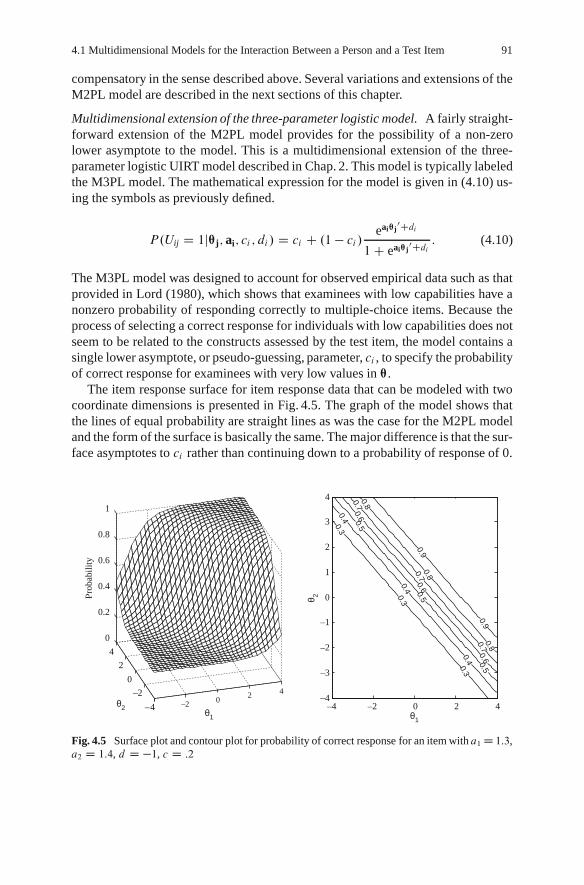
4.1 Multidimensional Models for the Interaction Between a Person and a Test Item 91
compensatory in the sense described above. Several variations and extensions of theM2PL model are described in the next sections of this chapter.
Multidimensional extension of the three-parameter logistic model. A fairly straight-forward extension of the M2PL model provides for the possibility of a non-zerolower asymptote to the model. This is a multidimensional extension of the three-parameter logistic UIRT model described in Chap. 2. This model is typically labeledthe M3PL model. The mathematical expression for the model is given in (4.10) us-ing the symbols as previously defined.
P.Uij D 1j™j; ai; ci ; di / D ci C .1 � ci /eai™j
0Cdi
1C eai™j0Cdi : (4.10)
The M3PL model was designed to account for observed empirical data such as thatprovided in Lord (1980), which shows that examinees with low capabilities have anonzero probability of responding correctly to multiple-choice items. Because theprocess of selecting a correct response for individuals with low capabilities does notseem to be related to the constructs assessed by the test item, the model contains asingle lower asymptote, or pseudo-guessing, parameter, ci , to specify the probabilityof correct response for examinees with very low values in ™.
The item response surface for item response data that can be modeled with twocoordinate dimensions is presented in Fig. 4.5. The graph of the model shows thatthe lines of equal probability are straight lines as was the case for the M2PL modeland the form of the surface is basically the same. The major difference is that the sur-face asymptotes to ci rather than continuing down to a probability of response of 0.
–4 –2 0 2 4–20
24
0
0.2
0.4
0.6
0.8
1
θ1
θ2
Prob
abili
ty
0.3
0.3
0.30.4
0.4
0.4
0.5
0.5
0.5
0.6
0.6
0.6
0.7
0.7
0.7
0.8
0.8
0.8
0.9
0.9
θ1
θ 2
–4 –2 0 2 4–4
–3
–2
–1
0
1
2
3
4
Fig. 4.5 Surface plot and contour plot for probability of correct response for an item with a1 D 1:3,a2 D 1:4, d D �1, c D :2

92 4 Multidimensional Item Response Theory Models
Multidimensional extension of the Rasch model. It is tempting to consider the mul-tidimensional extension of the Rasch model as simply the M2PL model with all ofthe a-parameters set to 1.0. This would be equivalent to the relationship betweenthe Rasch one-parameter logistic model and the two-parameter logistic model forthe UIRT case. However, an analysis of the consequences of setting all of thea-parameters in the M2PL model to 1.0 shows that this type of generalization ofthe UIRT case does not give a useful result.
The general form of the exponent of the M2PL model is given by
ai1�j1 C ai2�j2 C : : :C aim�jm C di : (4.11)
If all of the a-parameters are set equal to the same value, say ai�, they can be fac-tored from the expression in (4.11) to yield
ai�.�j1 C �j2 C : : :C �jm/C di : (4.12)
For Person j at any given moment, the �-coordinates are fixed and the sum of themtakes on a particular value that can be represented as ��. Substituting the sum of the�-coordinates into (4.12) yields ai��j� Cdj . Finally, if bi D �di=ai� , the exponentcan be represented as
ai�.�j� � bi /: (4.13)
If all of the ai� values are set to one, the exponent has the same form as the simpleUIRT Rasch model. The only difference is that the ability parameter is a value thatis the sum of coordinates rather than what is usually interpreted to be the level on asingle construct. Trying to create a multidimensional version of the Rasch model bysetting the a-parameters to 1.0 only yields a UIRT version of the Rasch model witha more complex definition for the person parameter.
The multidimensional generalization of the Rasch model is more complex. Theapproach that currently appears in the psychometric literature (Adams et al. 1997)is an adaptation of the general Rasch model presented in Chap. 3 (3.8). The modelas specified in Adams et al. (1997) is for the general case that includes both di-chotomously and polytomously scored test items. The general form of the modelis presented first using the notation from the original article. Then the simpler casefor dichotomously scored items is presented using the same notation as the othermodels presented in this book.
The expression for the full model is presented in (4.14). This model is for atest item that has the highest score category for Item i equal to Ki . The lowestscore category is 0. This implies that the number of score categories is Ki C 1. Forthe dichotomous case,Ki D 1 and there are two score categories, 0 and 1. The scorecategory is represented by k. The random variable Xik is an indicator variable thatindicates whether or not the observed response is equal to k on Item i . If the scoreis k, the indicator variable is assigned a 1 – otherwise, it is 0. For the dichotomouscase, if Xi1 D 1, the response to the item was a correct response and it was assigneda score of 1.

4.1 Multidimensional Models for the Interaction Between a Person and a Test Item 93
P.Xik D 1jA;B;Ÿ; ™/ D ebik™Caik0Ÿ
KiP
kD0ebik™Caik0Ÿ
; (4.14)
where A is a design matrix with vector elements aik that select the appropriate itemparameter for scoring the item; B is a scoring matrix with vector elements bik thatindicate the dimension or dimensions that are required to obtain the score of k onthe item; Ÿ is a vector of item difficulty parameters; and ™ is a vector of coordinatesfor locating a person in the construct space.
For the dichotomous case, using the same notation as the other models, the multi-dimensional Rasch model is given by
P.Uij D 1jai; di ; ™j/ D eai™j0Cdi
1C eai™j0Cdi ; (4.15)
where ai is a vector such that ai D bik and di is a scalar value equal to a0ikŸ. Note
that when k D 0 in (4.14) the exponent of e is 0 so that term of the sum in thedenominator is equal to 1.
Equation (4.15) and (4.5) appear to be identical. The difference between the twois the way that the ai vector is specified. In (4.5), ai is a characteristic of Item i thatis estimated from the data. In (4.15), ai is a characteristic of Item i that is speci-fied by the test developer. In the case of the model in (4.5), statistical estimationprocedures are used to determine the elements of ai that will maximize some cri-terion for model/data fit. Except for the usual monotonicity constraint that requiresthe values of the elements of ai be positive, the elements can take on any values.For the model in (4.15), the values are specified by the analyst and they typicallytake on integer values. Adams et al. (1997) specified two variations for the model– between item and within item dimensionality. For between item dimensionality,the ai-vector has elements that are all zeros except for one element that specifiesthe coordinate dimension that is measurement target for the item. That is, the testdeveloper specifies the dimension that is the target for the item. In a sense, the testdeveloper estimates the elements of the ai-vector rather than obtaining estimatesthrough the usual statistical estimation procedures.
For within item dimensionality, the ai-vector has more than one nonzero ele-ment. The test developer can indicate that performance on the test item is influencedby more than one of the coordinate dimensions. For the two-dimensional case,ai-vectors of [1 0] or [0 1] would indicate between item dimensionality. The firstvector would specify that the item was only affected by level on coordinate dimen-sion 1 and the second vector specifies that the item is only affected by level oncoordinate dimension 2. A specification for within item dimensionality might havea vector such as [1 1] indicating that the item is affected equally by both coordinatedimensions. Other alternatives such as [1 2] or [3 1] are possible. The quality ofthe fit of the model to the data will depend on how well the test developer specifiesthe values of the ai-vector.

94 4 Multidimensional Item Response Theory Models
–5
0
5
–4–2
02
40
0.2
0.4
0.6
0.8
1
θ1
[1 0]
θ2
Prob
abili
ty
–5
0
5
–4–2
02
40
0.2
0.4
0.6
0.8
1
θ1
[.5 1.5]
θ2
a b
Fig. 4.6 Two-dimensional Rasch model surfaces with ai D Œ1 0 and [.5 1.5] and di D 0
The reason for specifying the ai-vector rather than using statistical estimationmethods to determine the values is that the model then has observable sufficientstatistics for the person and item parameters (Rasch 1962). The sufficient statisticfor the ™-vector for a person is the sum of the ai-vectors for the items a personanswers correctly. The sufficient statistic that is related to the di -parameter is thesum over people of the ai-vectors for the correct responses to Item i . This is simplythe number of times Item i is answered correctly times ai.
The form of the item response surface for the multidimensional Rasch model fordichotomously scored items is the same as that shown in Fig. 4.3, but the orientationof the surface is dependent on the specification of values in the ai-vector. Figure 4.6shows surfaces for the two-dimensional case with ai-vectors [1 0] and [.5 1.5] anddi D 0 for both examples. The surface in panel a does not differentiate at all in prob-ability for differences along �2 – the item only measures �1. The item represented inpanel b has changes in probability for changes in �2 and slight changes along �1.
The model given in (4.14) has many other variations. Some of those will be de-scribed later in this chapter when multidimensional models for polytomously scoreditems are presented. The reader is referred to Adams et al. (1997) for a more detaileddescription of other variations of the model.
Multidimensional extension of the normal ogive model. As indicated in Chap. 3,much of the original work on MIRT was done using the normal ogive form to rep-resent the relationship between the location in the multidimensional space and theprobability of a correct response to a test item. The normal ogive form is still usedas the basis of statistical estimation programs. These programs and the underlyingstatistical methods are described in Chap. 6.

4.1 Multidimensional Models for the Interaction Between a Person and a Test Item 95
The general form for the multidimensional extension of the normal ogive model(Bock and Schilling 2003; McDonald 1999; Samejima 1974) is given by
P.Uij D 1j™j; ai; ci ; di / D ci C .1 � ci /1p2�
1Z
�zi .™j/
e�t2
2 dt; (4.16)
where zi .™j/ D ai™0j C di and the other symbols have been previously defined. If
ci D 0, the result is the normal ogive version of the multidimensional two-parameterlogistic model. That form of the model defines the probability of correct responsefor an item as the area under a standard normal distribution from –zi .™j/ to infinity.Because of the symmetry of the normal distribution, this is the same as the areabelow zi .™j/.
The form of the surface defined by (4.16) is essentially the same as that definedby (4.10). Camilli (1994) summarized the work on comparing the normal ogive andlogistic functions. He included the mathematical proof by Haley (1952) showingthat the normal distribution function and the logistic function differ by less than .01in probability when the constant 1.702 is included in the exponent of the logisticfunction. More explicitly, for z as defined above,
jˆ.z/ �‰.1:702z/j < :01 for � 1 < z < 1; (4.17)
where ˆ is the cumulative normal ogive function and ‰ is the cumulative logisticfunction.
For the parameters in (4.10) and (4.16) to have essentially the same meaning,the exponent of (4.10) has to be changed to 1:702.ai™
0j C di /. Multiplying by the
constant 1.702 changes the scale for the parameters in the logistic model, but has noother effect on the form of the surface. Figure 4.7 shows examples of the surfaces for
a c
–4–2
02
4
–4–2
02
40
0.2
0.4
0.6
0.8
1
θ1θ1
Normal Ogive
θ2
Prob
abili
ty
b
–4–2
02
4
–4–2
02
40
0.2
0.4
0.6
0.8
1
θ1
Logistic
θ2
Difference between Surfaces
0.002
–0.002
–0.002
–0.002
–0.002
0.002
0.0020.002
0.0050.005
0.005
0.005
–0.005
–0.005
–0.005
–0.005
θ 2
–4 –2 0 2 4–4
–3
–2
–1
0
1
2
3
4
Fig. 4.7 Normal ogive and logistic surfaces, and difference between the surfaces for a test itemwith a1 D :5, a2 D 1:5, d D 0, c D :2. Note that D D 1:702 is included in the exponent of thelogistic model

96 4 Multidimensional Item Response Theory Models
an item that can be modeled in two-dimensions using both the logistic and normalogive models. The difference in the two surfaces is also shown.
The surfaces shown in panels a and b are virtually indistinguishable. The contourplot of the differences between the two surfaces has less than .01 in all cases, and thedifferences were the same along the lines of equal probability. This indicates that thesurfaces have the same orientation to the coordinate axes – the lines of equal proba-bility are the same. Because of the close similarity of the surfaces defined by the twomodels, the parameters estimated from the models are often used interchangeablyas long as the 1.702 is included in the exponent of the logistic model.
All of variations of the logistic model presented in this chapter can also be im-plemented for the normal ogive model by modifying (4.16). If ci D 0, the resultis the multivariate generalization of the two-parameter normal ogive model. Thez-function can also be defined with prespecified ai vectors to yield a confirmatorymodel that is like the multivariate version of the Rasch model.
4.1.1.2 Partially Compensatory Extensions of UIRT Models
One of the continuing theoretical issues raised about the model presented in (4.5)is the compensatory nature of the model. If any m � 1 coordinates for a person arevery low, the person can still have a very high probability of correct response if themth coordinate is sufficiently high. Sympson (1978) argued that this hypothesizedcompensation is not realistic for some types of test items. He presents an example ofa mathematics test item that requires both arithmetic computation skills and readingskills. His example has similar characteristics to the test item presented at the begin-ning of this chapter. Sympson (1978) hypothesizes that a person with reading skillthat is very low will not be able to determine the problem that needs to be solved.The contention is that even if such a person had very high mathematics computationskills, they would not be able to determine the correct answer because of lack of un-derstanding of the problem. To model the situation he considered, Sympson (1978)proposed the following expression for the interaction between the person and thetest item, where all of the symbols have the same meaning as in previous equations.
P.Uij D 1j™j; ai;bi; ci / D ci C .1 � ci /
mY
`D1
e1:7ai`.�j`�bi`/
1C e1:7ai`.�j`�bi`/
!
: (4.18)
The expression in (4.18) has two main parts. The term on the far right is theproduct of terms that have the form of the 2PL UIRT model that was described inChap. 2. In a sense, each of these terms gives the probability of being successfulon one component of the item – for example, the reading or the mathematics com-ponents of the example item. These components of the test item are considered asindependent activities so that the probability of doing all of them correctly is theproduct of the probabilities of doing each part correctly. The other part of the ex-pression to the right of the equal sign provides a nonzero lower asymptote for the
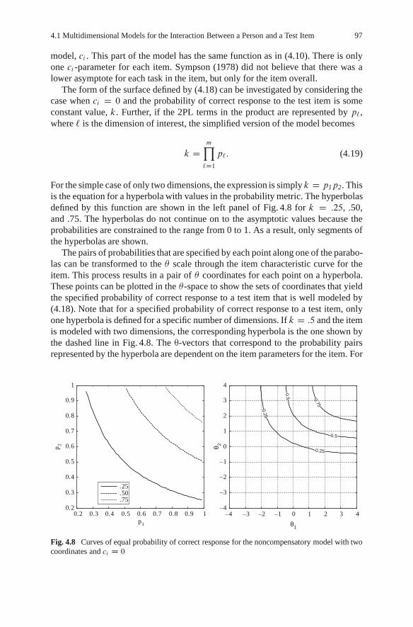
4.1 Multidimensional Models for the Interaction Between a Person and a Test Item 97
model, ci . This part of the model has the same function as in (4.10). There is onlyone ci -parameter for each item. Sympson (1978) did not believe that there was alower asymptote for each task in the item, but only for the item overall.
The form of the surface defined by (4.18) can be investigated by considering thecase when ci D 0 and the probability of correct response to the test item is someconstant value, k. Further, if the 2PL terms in the product are represented by p`,where ` is the dimension of interest, the simplified version of the model becomes
k DmY
`D1p`: (4.19)
For the simple case of only two dimensions, the expression is simply k D p1p2. Thisis the equation for a hyperbola with values in the probability metric. The hyperbolasdefined by this function are shown in the left panel of Fig. 4.8 for k D :25, .50,and .75. The hyperbolas do not continue on to the asymptotic values because theprobabilities are constrained to the range from 0 to 1. As a result, only segments ofthe hyperbolas are shown.
The pairs of probabilities that are specified by each point along one of the parabo-las can be transformed to the � scale through the item characteristic curve for theitem. This process results in a pair of � coordinates for each point on a hyperbola.These points can be plotted in the �-space to show the sets of coordinates that yieldthe specified probability of correct response to a test item that is well modeled by(4.18). Note that for a specified probability of correct response to a test item, onlyone hyperbola is defined for a specific number of dimensions. If k D :5 and the itemis modeled with two dimensions, the corresponding hyperbola is the one shown bythe dashed line in Fig. 4.8. The ™-vectors that correspond to the probability pairsrepresented by the hyperbola are dependent on the item parameters for the item. For
0.2 0.3 0.4 0.5 0.6 0.7 0.8 0.9 10.2
0.3
0.4
0.5
0.6
0.7
0.8
0.9
1
p1
p 2
.25
.50
.75
0.25
0.25
0.75
0.5
0.5
θ1
θ 2
–4 –3 –2 –1 0 1 2 3 4–4
–3
–2
–1
0
1
2
3
4
Fig. 4.8 Curves of equal probability of correct response for the noncompensatory model with twocoordinates and ci D 0
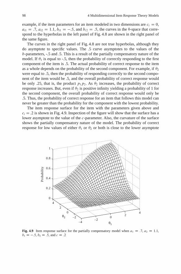
98 4 Multidimensional Item Response Theory Models
example, if the item parameters for an item modeled in two dimensions are ci D 0,ai1 D :7, ai2 D 1:1, bi1 D �:5, and bi2 D :5, the curves in the ™-space that corre-spond to the hyperbolas in the left panel of Fig. 4.8 are shown in the right panel ofthe same figure.
The curves in the right panel of Fig. 4.8 are not true hyperbolas, although theydo asymptote to specific values. The .5 curve asymptotes to the values of theb-parameters, -.5 and .5. This is a result of the partially compensatory nature of themodel. If �1 is equal to -.5, then the probability of correctly responding to the firstcomponent of the item is .5. The actual probability of correct response to the itemas a whole depends on the probability of the second component. For example, if �2were equal to .5, then the probability of responding correctly to the second compo-nent of the item would be .5, and the overall probability of correct response wouldbe only .25, that is, the product p1p2. As �2 increases, the probability of correctresponse increases. But, even if �2 is positive infinity yielding a probability of 1 forthe second component, the overall probability of correct response would only be.5. Thus, the probability of correct response for an item that follows this model cannever be greater than the probability for the component with the lowest probability.
The item response surface for the item with the parameters given above andci D :2 is shown in Fig. 4.9. Inspection of the figure will show that the surface has alower asymptote to the value of the c-parameter. Also, the curvature of the surfaceshows the partially compensatory nature of the model. The probability of correctresponse for low values of either �1 or �2 or both is close to the lower asymptote
–20
24
–4–2
02
40
0.2
0.4
0.6
0.8
1
θ1
θ2
Prob
abili
ty
Fig. 4.9 Item response surface for the partially compensatory model when a1 D :7, a2 D 1:1,b1 D �:5, b2 D :5, and c D :2

4.1 Multidimensional Models for the Interaction Between a Person and a Test Item 99
value. Only when both �-values are high does the model yield a high probability ofcorrect response.
Another unique feature of this model is that the interpretation of the item para-meters changes as the number of dimensions increase. Those familiar with UIRTprobably know that when � is equal to the difficulty parameter for the item, b, theprobability of correct response to the test item is .5 if there is no lower asymptoteparameter in the model. A simple example is if � D 0 and b D 0, the probability ofcorrect response is .5. The same is true for the compensatory model. If the ™-vectoris 0 and the d -parameter is 0, the probability of correct response to the item is .5when there is no lower asymptote parameter. However, that is not the case for thepartially compensatory model. If the ™-vector and the b-vector are both 0 for thetwo-dimensional case, the probability of correct response is .25. For the three di-mensional case, it is .125. In general, for the case when both the ™ and b-vectorsare 0, the probability of correct response is :5m, where m is the number of dimen-sions used in the model.
The value of a common b-parameter that yields a .5 probability of correct re-sponse depends on the corresponding a-parameter. However, it is useful to considerthe special case when ™ is the zero vector, all a-parameters are .588 (note that theconstant 1.7 is in the model), and the c-parameter is 0. If all the b-parameters arethe same, what must they be for the probability of correct response for the test itemto equal .5 for different numbers of dimensions? To get the answer, the left side of(4.18) is set to .5 and the equation is solved for b under the above constraints. Theresults are provided in Table 4.3.
The results in Table 4.3 show that as the number of dimensions increases, thevalue of the b-parameter must be reduced to maintain the same probability of correctresponse. This is a direct result of the fact that the model contains a product of theprobabilities of success on each component. Whenever the probability of successis less than 1.0, adding another component results in multiplying by a number lessthan 1.0. This reduces the overall probability of a correct response. To compensatefor this, the components must be easier as reflected by the reduced magnitude of theb-parameters.
The model presented in (4.18) is a multidimensional extension of the three-parameter logistic UIRT model. Whitely1 (1980b) suggested using a simplifiedversion of (4.18) to model the cognitive processes in test items. Maris (1995) also
Table 4.3 b-parameterrequired for a probabil-ity of correct responseof .5 for different numbersof dimensions
Number of dimensions b-parameter
1 0
2 �:883 �1:354 �1:665 �1:916 �2:10
1 Whitely now publishes under the name Embretson

100 4 Multidimensional Item Response Theory Models
suggested this model and labeled it the conjunctive Rasch model. The model is anextension of the one-parameter logistic model. This model is presented in (4.20).Although the terms in the product are equivalent to the Rasch UIRT model, the mul-tidimensional model does not match the requirements for a Rasch model becausethere is not an observable sufficient statistic for the person parameter vector. Adamset al. (1997) indicate that the model in (4.20) can be considered as a Rasch model ifit is considered as an item with 2m possible response categories. A vector of 0 s and1 s is developed to describe the success on each cognitive component of the model,and each of the possible vectors is considered as a response to the full item. Thisapproach is based on the assumption that success on the various cognitive compo-nents is independent. Whitely (1980b) also suggested a model of the same generalform that assumed that success on component ` was dependent on success on com-ponent ` � 1.
P.Uij D 1j™j;bi/ DmY
kD1
e.�jk�bik/
1C e.�jk�bjk/ : (4.20)
4.1.1.3 Comparison of Compensatory and Partially Compensatory Models
The models that combine the effect of multiple �s using a linear function in theexponent of the model (compensatory models) as in (4.5) and the ones that com-bine the �s through a product of terms (partially compensatory models) as in (4.18)are quite different in their philosophical underpinnings and in mathematical form.Some researchers (e.g., Maris 1995) may prefer one model over the other becauseit better matches hypotheses about how persons interact with the test items. Thepartially compensatory product models are consistent with the hypothesis that testitems have different parts related to different skills or knowledge and that overallsuccess requires success on each part. The compensatory models are more consis-tent with a more holistic view of the interaction of persons and test items. Personsbring all of their skills and knowledge to bear on all aspects of the items. Ulti-mately, the usefulness of the models will be determined by how accurately theyrepresent the responses from actual test items. Only a few studies were available atthe time this book was written that compared the fit of the two types of models tothe same data. One study that was identified, Bolt and Lall (2003), found that thecompensatory model fit item response data from an English usage test better thanthe partially compensatory model in (4.20). Note that this model does have all ofthe a-parameters set equal to 1. That study also compared the models on the fit todata generated from the other model. The compensatory model fit partially com-pensatory data almost as well as the partially compensatory model. The partiallycompensatory model did not fit the compensatory data very well.
The results reported by Spray et al. (1990) may provide some insight into theBolt and Lall (2003) results. They carefully selected parameters for the compen-satory model in (4.15) so that generated item response data would have the samecharacteristics such as internal consistency reliability, item difficulty distribution,and item discrimination as real test data. They then generated 2,000 ™-vectors and

4.1 Multidimensional Models for the Interaction Between a Person and a Test Item 101
Table 4.4 Item parameters for the partially compen-satory and compensatory models for the same test item
Partially compensatory model Compensatory model
Parameters Values Parameters Values
a1 1:26 a1 :90
a2 1:60 a2 1:31
b1 �:92 d �:67b2 �:15
–4
–2
0
2
4
–4–2
02
4
0
0.5
1
θ2
Both Surfaces on Same Axes
θ1
Prob
abili
ty
Contours of Difference Between Surfaces
0
0
0
0
0.2
0.2
0.2
0.2
0.4
0.4
0.6
0.6
θ1
θ 2
–4 –2 0 2 4–4
–3
–2
–1
0
1
2
3
4
Fig. 4.10 Comparison of partially compensatory and compensatory item response surfaces
computed the probability of correct response for each vector and the compensatoryparameters for each item. Then, assuming ™-vectors known, the parameters of thepartially compensatory model were estimated that minimized the squared differ-ences in probabilities of correct response. The results were item response surfacesthat gave the same p-values for each item assuming a standard bivariate normaldistribution of ™.
Table 4.4 gives the item parameters for the two models that gave best match to theitem response surfaces. The ci parameter was set to zero for the item. Figure 4.10shows the differences in the representation of the interaction between persons andthe test item in two different ways. The left panel of Fig. 4.10 shows the item re-sponse surfaces for the models on the same set of axes. The dark gray surface isfor the partially compensatory model and the white surface is for the compensatorymodel. The graph shows that the two surfaces intersect, with higher probabilities forthe partially compensatory surface ™-vectors when both elements are below 0.
The right panel in Fig. 4.10 shows a contour plot for the differences between thetwo surfaces. The enclosed curve labeled “0” represents the intersection of the two

102 4 Multidimensional Item Response Theory Models
surfaces. The probability of correct response is the same for the two models for™-vectors that fall on that curve. The other curves are labeled with the differencein probability of correct response for the two surfaces. Those contours show thatthe models give quite different probabilities of correct response for ™-vectors near(�3; 4) and (4;�1). In both of these regions of the ™-space, the compensatory modelgives probabilities of correct response that are over .6 higher than the partially com-pensatory model.
The two comparisons of the item response surfaces show that for ™vectors alongthe diagonal from (�4;�4) to (4, 4) there is little difference in the probability ofcorrect response for the two models. For real tests with �-elements that may bepositively correlated, the two models may give very similar results. It is only whenthe elements of the ™-vector are very different that the models predict different ratesof responding correctly to the test item.
The results for the test analyzed by Bolt and Lall (2003) suggest that the�-coordinates tend to function in a compensatory way for the items on the test.However, for other tests, the partially compensatory model may be more appropri-ate. Ultimately, empirical studies of the usefulness of the models for representingthe item response data are needed to determine which form of the model more ac-curately represents the interactions between persons and test items.
4.1.2 MIRT Models for Test Items with More Than Two ScoreCategories
Although test items that are scored using more than two score categories have beenused for a long time, the development of item response theory models for these itemtypes is a relatively new development. Chapter 2 provides a summary of some ofthese IRT models under the category polytomous IRT models (see Sect. 2.3). Thepolytomous IRT models have been extended to allow the person characteristics tobe represented by ™-vectors. Muraki and Carlson (1993) produced an extension ofthe graded response model, and there have been recent extensions of the generalizedpartial credit model (Yao and Schwarz 2006). The following sections of this chapterdescribe the extensions of the generalized partial credit, partial credit, and gradedresponse models. These models all fall under the label of compensatory models. Atthe time of the writing of this book, no partially compensatory polytomous modelshave been proposed.
4.1.2.1 Multidimensional Generalized Partial Credit Model
The multidimensional extension of the generalized partial credit (MGPC) model isdesigned to describe the interaction of persons with items that are scored with morethan two categories. The maximum score for Item i is represented by Ki . To beconsistent with the way dichotomous items are scored, the lowest score is assumed

4.1 Multidimensional Models for the Interaction Between a Person and a Test Item 103
to be 0 and there areKi C 1 score categories overall. The score assigned to a personon the item is represented by k D 0; 1; : : : ; Ki . The mathematical representationof the MGPC model is given by the following equation,
P.uij D kj™j / D ekai™
0
j�kP
uD0
ˇiu
KiP
vD0e
vai™0
j�vP
uD0
ˇiu
; (4.21)
where ˇiu is the threshold parameter for score category u, ˇi0 is defined to be 0,and all other symbols have there previously defined meaning. The representationof the model given here is a slight variation of the form given in Yao and Schwarz(2006).
There are two important differences between the equation for the MGPC modeland that for the GPC model given in (3.33). First, the model does not include sep-arate difficulty and threshold parameters. Second, because ™ is a vector and the ˇsare scalars, it is not possible to subtract the threshold parameter from ™. Instead, theslope/intercept form of the generalized partial credit model is used as the basis of themultidimensional generalization, a�Cd , but with the sign of the intercept reversed.The result is that the ˇs cannot be interpreted in the same way as the threshold pa-rameters in the UIRT version of the model. This will be discussed in more detailafter presenting the form of the item response surface.
The item response surfaces for the MGPC model for the case when theitem/person interaction can be represented in a space with two coordinate dimen-sions is presented in Fig. 4.11. The test item represented here has scores from 0 to 3.The item parameters for the model are ai D Œ1:2 :7 and ˇiu D 0; �2:5; �1:5; :5.
Figure 4.11 presents four surfaces – one for each possible item score. The darkestsurface to the left is for the score of 0. The probability of that score decreases as the
1
0.8
0.6
Pro
babi
lity
of S
core
0.4
0.2
–4 –3 –2 –1 0 1 2
Score 0Score 1Score 2Score 3
3 4–4
–2
0
2
4
q2
q1
0
Fig. 4.11 Item response surfaces for MGPC with item parameters ˇiu D 0, �2:5, �1:5, .5, andai D Œ1:2 :7

104 4 Multidimensional Item Response Theory Models
�-coordinate increases on either dimension. The surfaces for scores 1 and 2 firstincrease and then decrease as the �-coordinates increase. The surface for the scoreof 3 increases with an increase in any of the �-coordinates. The surfaces for thescores of 0 and 3 have upper asymptotes of 1 and lower asymptotes of 0. The othertwo surfaces have ridge-shaped forms with lower asymptotes of 0.
The intersections between the surfaces for adjacent score categories are over astraight line in the ™-plane. In general, the line is the set of points in the ™-planewhere the probabilities of obtaining the adjacent scores are equal. This set of pointscan be obtained by finding the solution to (4.22). This equation is specified bysetting the exponents in the numerator of (4.21) for adjacent score categories equalto each other.
kai™j0 �
kX
uD0ˇiu D .k C 1/ai™j
0 �kC1X
uD0ˇiu: (4.22)
Some algebraic manipulation results in the following solution for the intersectionbetween the kth and .k C 1/th surfaces. This is the equation for a line in them-dimensional space used to represent the item. Note that the only part of thisexpression that changes for different adjacent score categories is the intercept term,ˇ. As was the case for the UIRT version of the generalized partial credit model, thisparameter controls the location of the thresholds between score categories.
0 D ai™j0 � ˇi;kC1; k D 0; : : : ; k � 1: (4.23)
Equation (4.21) gives the expression for the probability of each score for a testitem. A surface that defines the expected score on the test item for a person with aparticular ™-vector is given by
E.uij j™j/ DKiX
kD0kP.uij D kj™j/: (4.24)
The surface defined by (4.24) for the item shown in Fig. 4.11 is given in Fig. 4.12.This surface has the appearance of the item response surface for a dichotomously
scored item for a compensatory model, but the upper asymptote for the surface is 3,the maximum score on the item. The MGPC is a compensatory model in the samesense as the UIRT version of the model in that a high value on �v can compensatefor a low value on �w resulting in a high expected score on the item. This effect canbe seen in the figure for the point (4, �4) that has an expected score near 3.
4.1.2.2 Multidimensional Partial Credit Model
There are a number of simplifications of the multidimensional version of the gener-alized partial credit model that have the special properties of the Rasch model. Thatis, they have observable sufficient statistics for the item- and person-parameters.Kelderman and Rijkes (1994) present the general form for one multidimensionalextension of the Rasch model to the polytomous test item case. Their model is
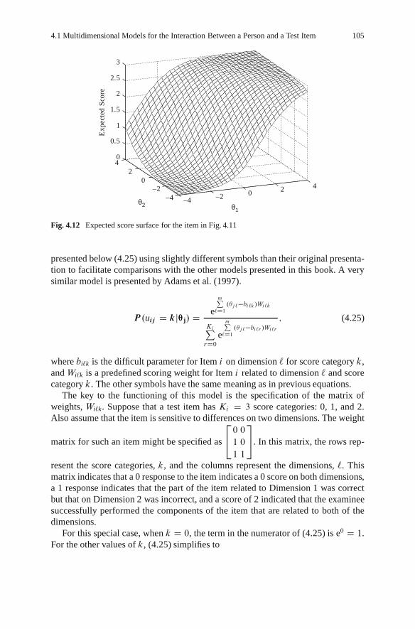
4.1 Multidimensional Models for the Interaction Between a Person and a Test Item 105
–4 –2 0 2 4–4
–20
240
0.5
1
1.5
2
2.5
3
θ1θ2
Exp
ecte
d Sc
ore
Fig. 4.12 Expected score surface for the item in Fig. 4.11
presented below (4.25) using slightly different symbols than their original presenta-tion to facilitate comparisons with the other models presented in this book. A verysimilar model is presented by Adams et al. (1997).
P.uij D kj™j/ D e
mP
`D1
.�j`�bi`k /Wi`k
KiP
rD0e
mP
`D1
.�j`�bi`r /Wi`r; (4.25)
where bi`k is the difficult parameter for Item i on dimension ` for score category k,and Wi`k is a predefined scoring weight for Item i related to dimension ` and scorecategory k. The other symbols have the same meaning as in previous equations.
The key to the functioning of this model is the specification of the matrix ofweights, Wi`k. Suppose that a test item has Ki D 3 score categories: 0, 1, and 2.Also assume that the item is sensitive to differences on two dimensions. The weight
matrix for such an item might be specified as
2
40 0
1 0
1 1
3
5. In this matrix, the rows rep-
resent the score categories, k, and the columns represent the dimensions, `. Thismatrix indicates that a 0 response to the item indicates a 0 score on both dimensions,a 1 response indicates that the part of the item related to Dimension 1 was correctbut that on Dimension 2 was incorrect, and a score of 2 indicated that the examineesuccessfully performed the components of the item that are related to both of thedimensions.
For this special case, when k D 0, the term in the numerator of (4.25) is e0 D 1.For the other values of k, (4.25) simplifies to

106 4 Multidimensional Item Response Theory Models
P.uij D kj™j/ D e
kP
`D1
.�j`�bi`k/
1CKiP
rD1e.�j`�bi`r/
; k D 1; : : : ; Ki : (4.26)
The developers of this model note that there is an indeterminacy in the estimation ofthe bi`k parameters so they set the parameters equal across the response categories,k D 1, 2; : : : , Ki . The items have different difficulty parameters for the differentdimensions, but the same for response categories within a dimension. This meansthat the item functions as a series of dichotomous items for each dimension with adifficulty for that dimension.
The item response surfaces for each score category for a test item scored 0, 1,or 2 using this model are shown in Fig. 4.13. This is for the two-dimensional casewith the scoring matrix given on the previous page. The bi`k parameters for the itemare �1 for dimension 1 and C1 for dimension 2. Careful study of Fig. 4.13 willshow that the surface for a score of zero is highest for ™-vector (�4;�4) and lowestfor the vector (4, 4). That score surface intersects with the surface for the score of 1along the line �1 D �1. The surface for a score of 1 is near 1 when the ™-vector is(4, �4) and it is near zero for the vector (�4, 4). It intersects with the surface for ascore of 2 along the line �2 D 1. Thus, for the region with �1 greater than �1 and �2
greater than 1, the score of 2 is the most likely score.The expected score surface for this test item is obtained by multiplying the score
category by the probability and summing over score categories. The expected scoresurface for the score response surfaces shown in Fig. 4.13 is presented in Fig. 4.14.
–4
–2
0
2
4
–4–2
02
4
0
0.5
1
θ1
θ2
Prob
abili
ty o
f Ite
m S
core
Score 0Score 1Score 2
Fig. 4.13 Item response surfaces for a Kelderman and Rijkes model for a test item that requirescapabilities on two dimensions to obtain a correct response – score categories of 0, 1, 2 – difficultyparameters �1 for dimension 1 and C1 for dimension 2

4.1 Multidimensional Models for the Interaction Between a Person and a Test Item 107
Exp
ecte
d Sc
ore
2
1.5
1
0.5
04
20
–4 –4–2–2
0
q1q2
24
Fig. 4.14 Expected score surface for the Kelderman and Rijkes model for the test item in Fig. 4.13
This surface has an expected score near 2 when levels on both �-coordinates are 4.The expected score drops as either � coordinate is reduced, but there is a levelingof the surface in the region around (4, �4). Examinees in this region have masteredthe first task in the test item, but have very low proficiency on the second task.Therefore, their expected score is 1.
This is a very interesting model because it acknowledges that the skills andknowledge needed to achieve the highest score on a test item may be differentthan those needed to achieve lower scores. The user of the model must confrontthe challenge of identifying the particular skills and knowledge needed for eachscore category. This might not be too great a problem for one item, but those skillsand knowledge categories need to generalize across the set of test items on a test. Atthis time there is not much in the research literature on the effect of misidentifyingthe required skills and knowledge for a test item.
4.1.2.3 Multidimensional Graded Response Model
Another approach to the multidimensional modeling of the responses to test itemswith more than two score categories was presented by Muraki and Carlson (1993).This model is a generalization of the unidimensional graded response model and ituses response functions that have the normal ogive form. As with the unidimensionalversion of this model, the multidimensional model assumes that successful accom-plishment of the task specified by the test item requires a number of steps andreaching step k requires success on step k � 1. This type of model is also appropri-ate for rating scales where a rating category subsumes all previous categories. Anexample is rating scale for the amount of time spent on a project. If a rating category

108 4 Multidimensional Item Response Theory Models
indicating one hour was spent on a project is selected, which means that all ratingcategories specifying less than one hour also apply.
The parameterization of the model given here considers the lowest score on Itemi to be 0 and the highest score to bemi . The probability of accomplishing k or moresteps is assumed to increase monotonically with an increase in any of the hypothet-ical constructs underlying the test as represented by the elements of the ™-vector.This is equivalent to dichotomizing the scale at k and scoring k or higher as a 1and below k as 0 and fitting a dichotomous model to the result. The probability ofaccomplishing k or more steps is modeled by a two-parameter normal ogive modelwith the person parameter defined as a linear combination of the elements in the™-vector weighted by discrimination parameters. The probability of receiving a spe-cific score, k, is the difference between the probability of successfully performingthe work for k or more steps and successfully performing the work for k C 1 ormore steps. If the probability of obtaining an item score of k or higher at a partic-ular ™-level is P�.uij D k j ™j/, then the probability that an examinee will receive ascore of k is
P.uij D k j ™j / D P �.uij D k j ™j / � P �.uij D k C 1 j ™j /; (4.27)
where P �.uij D 0 j ™j / D 1 because doing the work for step 0 or more is a cer-tainty for all examinees and P �.uij D mi C 1 j ™j / D 0 because it is impossibledo work representing more than category mi . The latter probability is defined sothat the probability of each score can be determined from (4.27). Samejima (1969)labels the terms on the right side of the expression as the cumulative category re-sponse functions and those on the left side of the expression as the category responsefunction.
The normal ogive form of the graded response model is given by
P.uij D k j ™j / D 1p2�
a0
i ™jCdikZ
a0
i �jCdi;kC1
e�t2
2 dt ; (4.28)
where k is the score on the item, 0, 1, : : :, mi , ai is a vector of item discriminationparameters, and dik is a parameter related to ease with which a person will reach thekth step of the item.
Note that the dik parameter has high positive values when it is relatively easy toobtain a particular score and large negative values when it is difficult to obtain aparticular score. The dik parameters have an inverse relationship with the scores forthe item. For score category 0, di0 D 1 and when the score category is mi C 1, avalue that is a point higher than actually exists on the score scale for the test item,di;miC1 D �1. Only the values of dik from k D 1 to mi are estimated in practice.
The probability of response category k can also computed from the difference oftwo integral expressions. This representation of the model is given in (4.29).

4.1 Multidimensional Models for the Interaction Between a Person and a Test Item 109
P.uij D k j ™j / D 1p2�
a0
i ™jCdikZ
�1e
�t2
2 dt � 1p2�
a0
i ™jCdi;kC1Z
�1e
�t2
2 dt: (4.29)
This representation of the model makes it clear that it is based on dichotomizing thescore scale for the item at different score values and using the normal ogive model todescribe the probability of obtaining a score at or above that value. The probabilityof a particular score value, k, is the difference between the probability of being k orhigher and k C 1 or higher.
Plots of the category response functions for a test item with four response cate-gories, 0, 1, 2, 3, are shown in Fig. 4.15. This test item has item parameters ai1 D 1:2,ai2 D :7, di1 D :5, di2 D � 1:5, and di3 D � 2:5. Careful study of the figure revealsthat as the �s increase, the probability of the score of 0 decreases and the score of3 increases. The intermediate scores of 1 and 2 increase, then decrease, as the �sincrease.
The expected score on the item is computed by multiplying the score by the prob-ability of the score. The expected score surface for the item shown in Fig. 4.15 is pre-sented in Fig. 4.16. The expected score is near 0 when the elements of the ™-vectorare both near �4 and it increases to near 3 when the elements of the ™-vector areboth near 4. Because the multidimensional graded response model is based on acompensatory multidimensional model, each of the response probability surfaceshas parallel equal probability contours. Therefore, the expected score surface alsohas parallel equal score contours.
The slope of this surface is dependent on both the magnitude of the elementsof the a-parameter vector and the amount of variation on the d -parameters. The
–4–2
02
4 –4–2
02
40
0.2
0.4
0.6
0.8
1
θ2θ1
Prob
abili
ty
Score 0Score 1Score 2Score 3
Fig. 4.15 Category response surfaces for an item with four score categories modeled by the gradedresponse model

110 4 Multidimensional Item Response Theory Models
–4 –3 –2 –1 0 1 2 3 4–4
–2
0
2
40
0.5
1
1.5
2
2.5
3
θ1
θ2
Exp
ecte
d Sc
ore
Fig. 4.16 Expected score surface for the item shown in Fig. 4.15
expected response surface is steeper when the variation in d -parameters is reduced.If the d -parameters are all equal, the item functions as a dichotomous item withscores of 0 and m.
The multidimensional graded response model has category response functionsthat appear similar to those from the multidimensional generalized partial creditmodel. A comparison of Figs. 4.11 and 4.15 will show the apparent similarity. Al-though, the models appear similar, they have different underlying scoring processesand work by van der Ark (2001) on the unidimensional versions of the models showthat it is possible to distinguish between data sets generated from the two models.
4.2 Future Directions for Model Development
Although many different kinds of MIRT models have been proposed, it is likelythat more models will be proposed as the interactions between persons and itemsbecome better understood. For example, it is likely that persons scoring performanceassessments such as writing samples consider different combinations of skills andknowledge when they assign scores representing different levels of performance.It may be that the difference between 0 and 1 on the rubric for scoring a writingsample may focus on simple writing mechanics, while differences between the topscore categories likely reflect differences in organization and style of writing. Suchshifts in the focus of the scoring rubrics suggest that there should be vectors ofa-parameters for each score boundary rather than a single a-parameter vector for theitem. A merger of the Kelderman and Rijkes (1994) model and the multidimensional

4.3 Exercises 111
versions of the generalized partial credit or graded response models may be neededto accurately represent scores from such rubrics.
It is also hypothesized that for some dichotomously scored items different ex-aminees have different solution strategies. A student who has recently studied thetopic that is the focus of the test item may be generating a response based on mem-ory of recent assignments. Another student may need to use problem solving skillsto determine how to approach the item. If situations can be identified where suchhypotheses can be supported, it may be necessary to merge latent class models andMIRT models. The latent class would define the solution strategy and the vectorsof �-elements would specify the skills and knowledge needed by each strategy.Model development is continuing and it is likely that new models or variations onthe existing models will appear in the research literature.
4.3 Exercises
1. Select a test item that you believe would be well modeled by a compensatorymodel and another test item that would be will modeled by a partially compensatorymodel. Describe why you believe each of the two items would be best representedby the different types of models.
2. A test item has three score categories and it is well fit by the multidimensionalgraded response model. The item has been calibrated assuming a three-dimensional™-space. The item parameter estimates for the item are given in the table below.Compute the probability of each score category for persons with the following two™-vectors – [�:5 .2 1] and [1:5-.7 0].
a1 a2 a3 d1 d2
.5 1 1.2 .8 �1:2
3. A dichotomously scored test item is well modeled by the compensatory logisticmodel using three coordinate dimensions. The a-parameter vector for the item is[.8 1.2 .3] and the d parameter is .5. What is the slope of the item response surfaceparallel to each coordinate axis at the point [0 0 0] in the ™-space?
4. A dichotomously scored test item is well modeled by the compensatory logis-tic model using two coordinate dimensions. The a-parameter vector for the item is[1.5 .5] and the d parameter is �1. Draw the lines in the ™-plane where the prob-ability of correct response for the item is .2 and .7. Determine the perpendiculardistance between the two lines. Do the same for an item with the same d para-meter, but with a-parameter vector [1.2 1.2]. For which item are the two lines closertogether? Explain why there is a difference in the distance for the two items.

112 4 Multidimensional Item Response Theory Models
5. A short quiz with five test items has been modeled using a MIRT model andthe probability of correct response for each item is predicted for a student in theclass. The probabilities for the five items are .9, .75, .60, .55, .5. After the quiz wasadministered the following scores were recorded for that student – 1 1 0 1 0. Theitem score vector and the probability vector have the items in the same order. Whatis the probability of the set of item scores for this student based on the MIRT model?What assumption of the model was important for computing the probability of theset of item scores?
6. Using the parameters for the two test items given in 4 above, compute the dis-tance from the origin of the ™-space to the .5 equiprobable contour for each item.
7. Does the data presented in Table 4.1 support the use of a compensatory orpartially compensatory MIRT model? Give the reasons for your conclusion usingspecific information from the table.
8. For a compensatory MIRT model with a lower asymptote parameter, c, that isnot zero, what probability of correct response corresponds to ™-vectors that meetthe condition a0™ C d D 0?
9. A test item is well modeled by the Rasch version of the partially compensatorymodel. The number of elements in the ™-vector is four and all of the b-parametersfor the item are equal. The observed probability of correct response for the item is.41 for a group of persons who all have ™-vectors equal to the 0 vector. What valueof the b-parameters is consistent with this information?

Chapter 5Statistical Descriptions of Itemand Test Functioning
The MIRT models in Chap. 4 provide mathematical descriptions of the interactionsof persons and test items. Although the parameters of these models summarize thecharacteristics of the items, the vectors of item parameters sometimes lack intuitivemeaning. This chapter provides other statistical ways of describing the functioningof test items that may more clearly indicate the value of the test items for deter-mining the location of individuals in the multidimensional ™-space. The ways ofdescribing test item characteristics given here are direct extensions of the descrip-tive information for UIRT models described in Chap. 2.
5.1 Item Difficulty and Discrimination
The UIRT measures of item difficulty and discrimination are directly related to thecharacteristics of the item characteristic curve (ICC). The difficulty parameter in-dicates the value of � that corresponds to the point of steepest slope for the ICC.The discrimination parameter is related to the slope of the ICC where it is steepest.These two descriptive statistics for test items can be generalized to the MIRT case,but there are some complexities to the process. The slope of a surface is dependenton the direction of movement along the surface so the point of steepest slope de-pends on the direction that is being considered. For example, the contour plot of theitem response surface for a test item that is well modeled by the multidimensionalextension of the two-parameter logistic (M2pl) model is shown in Fig. 5.1. The solidarrow in the figure shows a direction that is parallel to the equi-probable contoursfor the surface, the set of points in the ™-space that yield the same probability ofcorrect response to the test item. Over the length of the arrow, there is no change inprobability so the slope in that direction is zero. The dashed arrow is in a directionwith substantial change in probability – .4 over the length of the arrow. Because thelength of the arrow is about one unit, the slope in that direction is about .4.
At each point in the ™-space, there is a direction that has the maximum slopefrom that point. If the entire ™-space is considered and the slopes in all directionsat each point are evaluated, there is a maximum slope overall for the test item. Thevalue of the maximum slope would be a useful summary of the capabilities of the
M.D. Reckase, Multidimensional Item Response Theory, Statistics for Socialand Behavioral Sciences, DOI 10.1007/978-0-387-89976-3 5,c� Springer Science+Business Media, LLC 2009
113
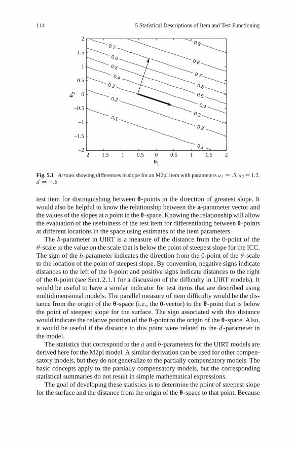
114 5 Statistical Descriptions of Item and Test Functioning
0.1
0.1
0.2
0.2
0.3
0.3
0.4
0.4
0.5
0.5
0.6
0.6
0.7
0.7
0.8
0.9
θ1
θ 2
−2 −1.5 −1 −0.5 0 0.5 1 1.5 2−2
−1.5
−1
−0.5
0
0.5
1
1.5
2
Fig. 5.1 Arrows showing differences in slope for an M2pl item with parameters a1 D :5, a2 D 1:2,d D �:6
test item for distinguishing between ™-points in the direction of greatest slope. Itwould also be helpful to know the relationship between the a-parameter vector andthe values of the slopes at a point in the ™-space. Knowing the relationship will allowthe evaluation of the usefulness of the test item for differentiating between ™-pointsat different locations in the space using estimates of the item parameters.
The b-parameter in UIRT is a measure of the distance from the 0-point of the�-scale to the value on the scale that is below the point of steepest slope for the ICC.The sign of the b-parameter indicates the direction from the 0-point of the �-scaleto the location of the point of steepest slope. By convention, negative signs indicatedistances to the left of the 0-point and positive signs indicate distances to the rightof the 0-point (see Sect. 2.1.1 for a discussion of the difficulty in UIRT models). Itwould be useful to have a similar indicator for test items that are described usingmultidimensional models. The parallel measure of item difficulty would be the dis-tance from the origin of the ™-space (i.e., the 0-vector) to the ™-point that is belowthe point of steepest slope for the surface. The sign associated with this distancewould indicate the relative position of the ™-point to the origin of the ™-space. Also,it would be useful if the distance to this point were related to the d -parameter inthe model.
The statistics that correspond to the a and b-parameters for the UIRT models arederived here for the M2pl model. A similar derivation can be used for other compen-satory models, but they do not generalize to the partially compensatory models. Thebasic concepts apply to the partially compensatory models, but the correspondingstatistical summaries do not result in simple mathematical expressions.
The goal of developing these statistics is to determine the point of steepest slopefor the surface and the distance from the origin of the ™-space to that point. Because

5.1 Item Difficulty and Discrimination 115
−3 −2 −1 0 1 2 3−3
−2
−1
0
1
2
3
θ1
θ 2
(1.5, 2.2)
a1 = 56
Fig. 5.2 Polar coordinate representation of a point in a two-dimensional ™-space – the length ofarrow is 2.66 � -coordinate units
this conceptualization uses the distance from the origin of the ™-space as a ref-erence point for the measure of item difficulty, it is helpful to reparameterize theM2pl model using a polar coordinate representation. That is, instead of representingeach point in the ™-space by a vector of �-coordinates, each point is representedby a vector of angles from each coordinate axis and a distance from the origin.A two-dimensional representation of this reparameterization is given in Fig. 5.2.The same conceptual framework can be used to generalize the reparameterization toan n-dimensional space.
In Fig. 5.2, the location of a point in the ™-space is indicated by the two coordi-nates, �1 D 1:5 and �2 D 2:2. That same point can also be represented by a distance(i.e., the bold arrow) of 2.66 �-units and a direction of 56ı from the �1-axis. The dis-tance is computed using the standard distance formula and the angle is determinedfrom the right triangle trigonometric formula for the cosine of an angle. In this two-dimensional case, the angle between the arrow and the �2-axis can be determinedby subtraction as 90 � 56D 34ı. In m dimensions, m � 1 angles can be computedfrom the �-coordinates using trigonometric relationships. The mth angle is mathe-matically determined because the sum of squared cosines must equal 1. Given thedistance to the point and the directions from the axes, the values of the coordinatesof the point on each of the axes can be recovered using the trigonometric relationship
�v D � cos ˛v; (5.1)
where �v is the coordinate of the point on dimension v, � is the distance from the ori-gin to the point, and ˛v is the angle between the vth axis and the line from the originto the point.
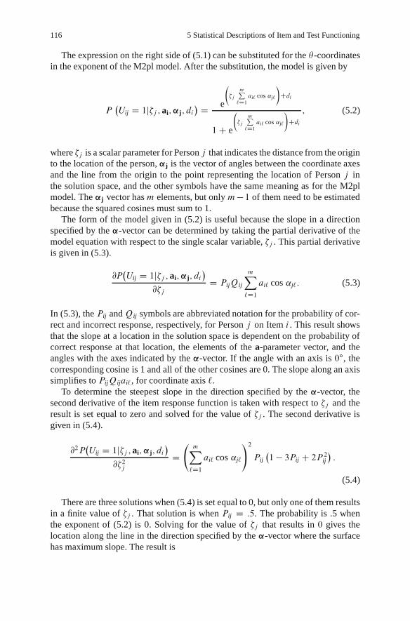
116 5 Statistical Descriptions of Item and Test Functioning
The expression on the right side of (5.1) can be substituted for the �-coordinatesin the exponent of the M2pl model. After the substitution, the model is given by
P�Uij D 1j�j ; ai;’j; di
D e
�jmP
`D1
ai` cos ˛j`
!
Cdi
1C e
�jmP
`D1
ai` cos ˛j`
!
Cdi; (5.2)
where �j is a scalar parameter for Person j that indicates the distance from the originto the location of the person, ’j is the vector of angles between the coordinate axesand the line from the origin to the point representing the location of Person j inthe solution space, and the other symbols have the same meaning as for the M2plmodel. The ’j vector has m elements, but only m� 1 of them need to be estimatedbecause the squared cosines must sum to 1.
The form of the model given in (5.2) is useful because the slope in a directionspecified by the ’-vector can be determined by taking the partial derivative of themodel equation with respect to the single scalar variable, �j . This partial derivativeis given in (5.3).
@P�Uij D 1j�j ; ai;’j; di
@�jD PijQij
mX
`D1ai` cos ˛j`: (5.3)
In (5.3), the Pij andQij symbols are abbreviated notation for the probability of cor-rect and incorrect response, respectively, for Person j on Item i . This result showsthat the slope at a location in the solution space is dependent on the probability ofcorrect response at that location, the elements of the a-parameter vector, and theangles with the axes indicated by the ’-vector. If the angle with an axis is 0ı, thecorresponding cosine is 1 and all of the other cosines are 0. The slope along an axissimplifies to PijQijai`, for coordinate axis `.
To determine the steepest slope in the direction specified by the ’-vector, thesecond derivative of the item response function is taken with respect to �j and theresult is set equal to zero and solved for the value of �j . The second derivative isgiven in (5.4).
@2P�Uij D 1j�j ; ai;’j; di
@�2jD
mX
`D1ai` cos ˛j`
!2Pij�1 � 3Pij C 2P 2
ij
:
(5.4)
There are three solutions when (5.4) is set equal to 0, but only one of them resultsin a finite value of �j . That solution is when Pij D :5. The probability is .5 whenthe exponent of (5.2) is 0. Solving for the value of �j that results in 0 gives thelocation along the line in the direction specified by the ’-vector where the surfacehas maximum slope. The result is

5.1 Item Difficulty and Discrimination 117
�dimP
`D1ai` cos ˛j`
; (5.5)
where all of the symbols have been previously defined. The location of the point ofmaximum slope along a particular axis is simply �d=ai` because all of the cosineswill be 0 except for the axis ` being considered. For that axis, the cosine is 1.
Substituting the expression in (5.5) for �j in (5.2) results in a probability of acorrect response of .5 for a person located along the line from the origin at the pointthat gives the steepest slope. As a result, the value of the slope at the point of steepestslope in the direction specified by the ’-vector is
1
4
mX
`D1ai` cos ˛j`: (5.6)
To determine the direction of steepest slope from the origin of the ™-space, theexpression in (5.6) is differentiated with respect to cos ’ and solved for 0. This isdone under the constraint that the sum of the squared cosines is equal to 1. The resultis the system of equations given in (5.7).
ai` � aimcos ˛i`
cos ˛imD 0; for ` D 1; 2; : : : ; m � 1; (5.7)
where cos2 ˛im D 1 �m�1PkD1
cos2 ˛ik. The solution for the system of equations is
given by
cos ˛i` D ai`smP
kD1a2ik
: (5.8)
The corresponding angles are given by taking the arccosine of the cosine of ˛. Theseangles and cosines are characteristics of the item. They indicate the direction fromthe origin of the ™-space to the point in the ™-space that has the greatest slope con-sidering all possible directions. The cosines specified by (5.8) are sometimes calleddirection cosines.
The distance from the origin to the point of steepest slope in the direction spec-ified by (5.8) can be obtained by substituting the results of (5.8) for the cos ˛ in(5.5). The result is
Bi D �dismP
kD1a2ik
: (5.9)
The symbol Bi is used here to represent the multidimensional difficulty of the testitem. Sometimes this item characteristic is represented by MDIFF, butB is used hereto more clearly make the connection to the unidimensional b-parameter because it
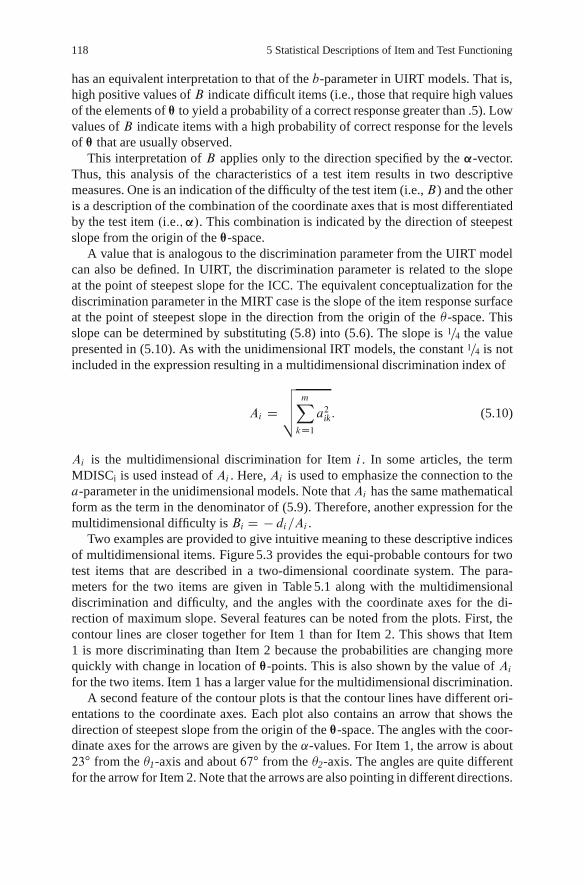
118 5 Statistical Descriptions of Item and Test Functioning
has an equivalent interpretation to that of the b-parameter in UIRT models. That is,high positive values of B indicate difficult items (i.e., those that require high valuesof the elements of ™ to yield a probability of a correct response greater than .5). Lowvalues of B indicate items with a high probability of correct response for the levelsof ™ that are usually observed.
This interpretation of B applies only to the direction specified by the ’-vector.Thus, this analysis of the characteristics of a test item results in two descriptivemeasures. One is an indication of the difficulty of the test item (i.e.,B) and the otheris a description of the combination of the coordinate axes that is most differentiatedby the test item .i:e:;’/. This combination is indicated by the direction of steepestslope from the origin of the ™-space.
A value that is analogous to the discrimination parameter from the UIRT modelcan also be defined. In UIRT, the discrimination parameter is related to the slopeat the point of steepest slope for the ICC. The equivalent conceptualization for thediscrimination parameter in the MIRT case is the slope of the item response surfaceat the point of steepest slope in the direction from the origin of the �-space. Thisslope can be determined by substituting (5.8) into (5.6). The slope is 1=4 the valuepresented in (5.10). As with the unidimensional IRT models, the constant 1=4 is notincluded in the expression resulting in a multidimensional discrimination index of
Ai Dvuut
mX
kD1a2ik: (5.10)
Ai is the multidimensional discrimination for Item i . In some articles, the termMDISCi is used instead of Ai . Here, Ai is used to emphasize the connection to thea-parameter in the unidimensional models. Note that Ai has the same mathematicalform as the term in the denominator of (5.9). Therefore, another expression for themultidimensional difficulty is Bi D � di=Ai .
Two examples are provided to give intuitive meaning to these descriptive indicesof multidimensional items. Figure 5.3 provides the equi-probable contours for twotest items that are described in a two-dimensional coordinate system. The para-meters for the two items are given in Table 5.1 along with the multidimensionaldiscrimination and difficulty, and the angles with the coordinate axes for the di-rection of maximum slope. Several features can be noted from the plots. First, thecontour lines are closer together for Item 1 than for Item 2. This shows that Item1 is more discriminating than Item 2 because the probabilities are changing morequickly with change in location of ™-points. This is also shown by the value of Aifor the two items. Item 1 has a larger value for the multidimensional discrimination.
A second feature of the contour plots is that the contour lines have different ori-entations to the coordinate axes. Each plot also contains an arrow that shows thedirection of steepest slope from the origin of the ™-space. The angles with the coor-dinate axes for the arrows are given by the ˛-values. For Item 1, the arrow is about23ı from the �1-axis and about 67ı from the �2-axis. The angles are quite differentfor the arrow for Item 2. Note that the arrows are also pointing in different directions.

5.1 Item Difficulty and Discrimination 119
0.1
0.1
0.1
0.2
0.2
0.2
0.3
0.3
0.3
0.4
0.4
0.4
0.5
0.5
0.5
0.6
0.6
0.6
0.7
0.7
0.7
0.8
0.8
0.8
0.9
0.9θ1
θ 2Item 1
−4 −2 0 2 4−4
−3
−2
−1
0
1
2
3
4Item 2
0.1
0.1
0.2
0.2
0.3
0.3
0.4
0.4
0.5
0.5
0.6
0.6
0.7
0.7
0.8
0.8
0.9
0.9
θ1θ 2
−4 −2 0 2 4−4
−3
−2
−1
0
1
2
3
4
Fig. 5.3 Representation of the characteristics of the items with parameters in Table 5.1
Table 5.1 Item parameters and multidimensional statistics for two test items
Item a1 a2 d A B ˛1 ˛2
1 1:2 .5 �1:5 1.30 1:15 22.62 67.382 :6 1 :9 1.17 �:77 59.04 30.96
The arrows stretch from the origin of the ™-space to the line of the .5-probabilitycontour. When the arrow is in the lower left quadrant of the space, the item is fairlyeasy. When the arrow is in the upper right quadrant, the item is fairly hard. The onlyway that the arrow will point in the direction of one of the other quadrants is if oneof the a-parameters is negative. The length and direction of the arrow is given byBi .Negative values generally indicate easy items and positive values hard items.
If the item response surfaces for multiple items are plotted as equi-probable con-tour plots on the same set of axes, the characteristics of the individual items will bedifficult to discern because of the number of intersecting equi-probable lines. Oneway to show the same information in a less cluttered way is to represent each itemby an arrow with the base of the arrow at the point of maximum slope along a linefrom the origin of the ™-space. The arrow points up slope in the direction along theline from the origin. The length of the arrow can be used to represent the discrimi-nating power,Ai , for the item. The distance from the origin to the base of the arrowindicates the difficulty,Bi , for the item and the direction, ’{, of the arrow shows thedirection of greatest positive change in slope for the item. This type of representationfor the two items in Table 5.1 is given in Fig. 5.4. Using these conventions, a numberof items can be displayed graphically when the number of coordinate axes is two orthree. Figure 5.5 gives the arrow representation for 45 items in a three-dimensionalspace. This representation of the items makes it clear that the items form three fairlydistinct sets that tend to have the steepest slope in the same direction.

120 5 Statistical Descriptions of Item and Test Functioning
Fig. 5.4 Representationof items with parametersin Table 5.1 as arrows
−3 −2 −1 0 1 2 3−3
−2
−1
0
1
2
3
θ1
θ 2
−1 –0.5 0 0.5 1 1.5−1−0.50
0.51
1.5−1
−0.5
0
0.5
1
1.5
θ1
θ2
θ 3
Fig. 5.5 Representation of 45 items by arrows in a three-dimensional space
The description of test items using the concepts of multidimensional difficulty,multidimensional discrimination, and direction of steepest slope in the multidimen-sional space can also be used with polytomous test items. Muraki and Carlson(1993) derive these statistics for the multidimensional graded response model. The

5.2 Item Information 121
development results in the same expressions for multidimensional discrimination,Ai , and the vector of angles, ’. They also developed the equivalent to (5.9) for thestep difficulty for an item (see (4.28)).
Bik D �diksmP
`D1a2i`
; (5.11)
where Bik is the step difficulty for the kth step of the graded response item and dik
is the step parameter as defined in the model. The other terms have been previouslydefined.
The same procedures can be used to define the multidimensional statistics forthe item whenever the exponential term in the model is in the form a™0 C d . Thisis also the case when the limits of integration for a normal ogive model have thesame form. Partially compensatory models do not have this form; therefore, thesestatistical descriptions of characteristics of the test items do not apply to test itemsthat are described by partially compensatory models. It may be possible to derivesimilar statistics for test items model by the partially compensatory models, but theyhave not been developed at the time this book was written.
5.2 Item Information
The concept of item information that is used in UIRT can also be generalized tothe multidimensional case. The definition of information in the multidimensionalcase is the same as that given in (2.42) for the unidimensional case – the squaredslope of the regression of the item score on the ™ divided by the variance of theitem score at � . There is a complication, however. At each point in the ™-space,the slope of the multidimensional item response surface differs depending on thedirection of movement from the point. The two arrows in Fig. 5.1 give examplesof the differences in slope for movements in different directions. The solid arrowshows movement in a direction that has a slope of 0. The dashed arrow has a muchhigher positive slope. This implies that the information provided by a test item aboutthe difference between nearby points in the ™-space depends on the orientation ofthe points (i.e., the direction of movement from one point to the other).
To accommodate the change in slope with direction taken from a point in the™-space, the definition of item information is generalized to
I’.™/ D Œr’P.™/2
P.™/Q.™/; (5.12)
where ’ is the vector of angles with the coordinate axes that defines the directiontaken from the ™-point, r’ is the directional derivative or gradient, in the direc-tion ’, and the other symbols as previously defined. Equation (5.12) represents the

122 5 Statistical Descriptions of Item and Test Functioning
information for one item at one location in the ™-space, so the item and person sub-scripts have not been included to more clearly show the general structure of theexpression.
The directional derivative for the item response surface is given by
r’P.™/ D @P.™/
@�1cos ˛1 C @P.™/
@�2cos ˛2 C � � � C @P.™/
@�mcos ˛m: (5.13)
If the MIRT model being considered is the multidimensional extension of thetwo-parameter logistic model given in (4.5), the directional derivative is
r’P.™/ D a1P.™/Q.™/ cos ˛1C a2P.™/Q.™/ cos ˛2 C � � � C amP.™/Q.™/ cos ˛m: (5.14)
This expression can be presented more compactly as
r’P.™/ D P.™/Q.™/
mX
vD1av cos ˛v: (5.15)
Substituting (5.15) into (5.12) yields
I’.™/ D
�P.™/Q.™/
mP
vD1av cos ˛v
�2
P.™/Q.™/D P.™/Q.™/
mX
vD1av cos ˛v
!2:
(5.16)
When the MIRT model contains only two dimensions, the information in thedirection specified by the ’-vector can be represented by an information surface.The height of the surface above the �-plane indicates the amount of informationat each location in the plane. Information surfaces for the test item represented inthe contour plot shown in Fig. 5.1 are shown in Fig. 5.6. The surfaces show theinformation in three directions – angles of 0, 67.38, and 90ı with the �1-axis.
The angle of 67:38ı is the direction from the �1-axis when the item responsesurface has the steepest slope along a line from the origin of the space. In all threecases, the information surfaces have the shape of a ridge that has its highest regionover the .5 equiprobable contour line for the test item. That is the line in the ™-spacewhere the slope of the item response surface is the greatest as well. Of all of thepossible directions in the space, the direction of steepest slope has the highest ridgefor the information function. The low maximum height for the ridge in the panelon the left of Fig. 5.6 shows that the test item is relatively ineffective at distinguish-ing nearby points when the direction between the points is parallel to the �1-axis.However, the test item is quite effective at distinguishing points on either side ofthe .5 equiprobable contour in the direction of steepest slope for the item responsesurface – 67:38ı to the �1-axis. This is shown by the high ridge in the middle panel

5.2 Item Information 123
0
5
-4-20240
0.1
0.2
0.3
0.4
0.5
θ1
0 Degrees
θ2
θ1
θ2
θ1
θ2
Info
rmat
ion
0
5
-4-20240
0.1
0.2
0.3
0.4
0.5
67.38 Degrees
0
5
-4-20240
0.1
0.2
0.3
0.4
0.5
90 Degrees
Fig. 5.6 Information surfaces for a M2PL test item with a1 D :5, a2 D 1:2, and d D �:6 in threedirections
of Fig. 5.6. The capability of the item for distinguishing in a direction parallel to the�2-axis is between the other two directions as shown by the right panel in the figure.The maximum height of the surface is between the maximum heights of the surfacesfor the other two directions.
If the direction of steepest slope from (5.8) is substituted for the cos ˛k in (5.16),the result is the information for the test item in the direction of maximum slope.That expression is given by
I˛ max.™/ D P.™/Q.™/
mX
kD1a2k D P.™/Q.™/A2; (5.17)
where A is the multidimensional discrimination for the item. In this case, the in-formation function has exactly the same form as that for the two-parameter logisticmodel described in Chap. 2. For the example in Fig. 5.6, A D 1:3 and because theterm P.™/Q.™/ has its maximum when P.™/ D :5, the maximum information is:5 � :5 � 1:32 D :425.
Because the information surface is different in every direction that is selected, it isdifficult to get a sense of the overall information provided by an item. One approachto addressing this issue was given by Reckase and McKinley (1991). For a grid ofpoints selected in the ™-space, the information was determined in directions fromthe �1-axis in 10ı increments. The results were plotted as lines radiating from the™-points in the selected directions with the length of the line indicating the amountof information. These plots have sometimes been labeled “clam shell” plots becausethe sets of lines often look like the back of a clam shell. Figure 5.7 shows a clamshell plot for the information provided by the test item shown in Fig. 5.6.
Careful examination of Fig. 5.7 will show that the lines are longest for ™-pointsthat fall near the .5 equiprobable contour line and that the longest line in each set oflines is at 70ı, the angle closest to the direction of maximum slope from the originof the ™-space. When the ™-points are far from the .5 contour line, the informa-tion is very low and the amount is represented by a point on the graph. Clam shell
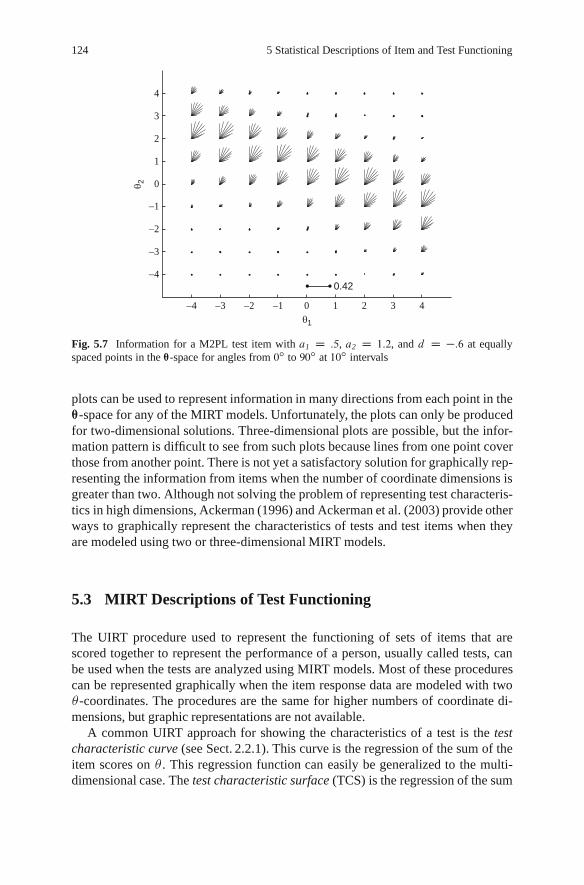
124 5 Statistical Descriptions of Item and Test Functioning
−4 −3 −2 −1 0 1 2 3 4
−4
−3
−2
−1
0
1
2
3
4
θ1
θ 2
0.42
Fig. 5.7 Information for a M2PL test item with a1 D :5, a2 D 1:2, and d D �:6 at equallyspaced points in the ™-space for angles from 0ı to 90ı at 10ı intervals
plots can be used to represent information in many directions from each point in the™-space for any of the MIRT models. Unfortunately, the plots can only be producedfor two-dimensional solutions. Three-dimensional plots are possible, but the infor-mation pattern is difficult to see from such plots because lines from one point coverthose from another point. There is not yet a satisfactory solution for graphically rep-resenting the information from items when the number of coordinate dimensions isgreater than two. Although not solving the problem of representing test characteris-tics in high dimensions, Ackerman (1996) and Ackerman et al. (2003) provide otherways to graphically represent the characteristics of tests and test items when theyare modeled using two or three-dimensional MIRT models.
5.3 MIRT Descriptions of Test Functioning
The UIRT procedure used to represent the functioning of sets of items that arescored together to represent the performance of a person, usually called tests, canbe used when the tests are analyzed using MIRT models. Most of these procedurescan be represented graphically when the item response data are modeled with two�-coordinates. The procedures are the same for higher numbers of coordinate di-mensions, but graphic representations are not available.
A common UIRT approach for showing the characteristics of a test is the testcharacteristic curve (see Sect. 2.2.1). This curve is the regression of the sum of theitem scores on � . This regression function can easily be generalized to the multi-dimensional case. The test characteristic surface (TCS) is the regression of the sum

5.3 MIRT Descriptions of Test Functioning 125
of the item scores on the ™-vector. The mathematical expression for the test charac-teristic surface, or TCS, is exactly the same as for UIRT models (see (2.38)) exceptthat the expectation is conditioned on the ™-vector instead of the unidimensionalvalue of � . The MIRT expression for the TCS for a test composed of dichotomouslyscored test items is given by
E�yj j™j
D E
nX
iD1uijj™j
!
DnX
iD1E�uijj™j
DnX
iD1P�uijj™j
: (5.18)
The TCS is simply the sum of the item characteristic surfaces for the items in thetest. For tests composed of polytomously scored items, or mixtures of dichoto-mously and polytomously scored items, all of the terms in (5.18) still hold exceptthe one at the far right. The TCS is the sum of the expected scores on the test itemsincluded in the test conditional on the ™-vectors.
An example of the TCS for a test is given using the item parameter esti-mates provided in Table 5.2. These parameter estimates were obtained from atwo-dimensional solution using the program NOHARM. Detailed information aboutthis program is given in Chap. 6. The TCS for this set of items is shown using twodifferent graphic representations, (a) and (b), in Fig. 5.8. For points in the ™-spacenear .�4;�4/, the expected number-correct score on the set of test items is near 0.With increase in either �-coordinate, the expected number-correct score increasesuntil it approaches the maximum of 20 near .4; 4/. The surface appears similar to anitem characteristic surface (see panel a), but the equal score contours are not straightlines (see panel b) as they are for an item characteristic surface (Fig. 4.5).
Another way of summarizing the characteristics of the set of test items in a testis to indicate the orientation of the unidimensional �-scale in the multidimensional
4
−4
−3
−2
−1
0
1
2
3
4
4 6
8 1012
14
1618
18
14
16
1210
864
2
2 4 68 10
12
−4 −2 0 2 4
2
0
−2
−4 −4−2
0
q2
q 2
q1
q12
4Exp
ecte
d N
umbe
r-C
orre
ct S
core
0
5
10
15
a b
20
Fig. 5.8 Test characteristic surface for the test items in Table 5.2. Plot (a) shows the surface andplot (b) shows the equal score contours for the surface

126 5 Statistical Descriptions of Item and Test Functioning
Table 5.2 Item parameterestimates from a two-dimensional compensatorymodel
Item number a1 a2 d
1 :79 1:36 �:902 :93 1:38 �1:203 :58 :38 1:00
4 :87 :87 �:975 :83 :79 �1:086 :31 :99 �1:537 :60 :48 �:618 :60 :87 �:609 1:64 :15 1:24
10 1:11 1:30 �:6911 :53 :97 �1:3112 1:26 :39 :92
13 2:37 :00 2:49
14 1:17 1:76 �:0615 :96 1:26 �:4816 :56 :46 �:8217 1:17 :20 1:11
18 :63 :26 :66
19 1:01 :47 �:1520 :81 :77 �1:08
space. This is the line in the multidimensional space that represents the unidimen-sional scale. The projections of the ™-points in the multidimensional space givesan estimate of the unidimensional � that would result if the response data from thetest items were analyzed using a unidimensional IRT model. Wang (1985, 1986)derived that the unidimensional �-line corresponding to the �-estimates from a setof test items was related to the characteristics of the matrix of discrimination para-meters for the compensatory MIRT model, a. The orientation of the unidimensionalline in the ™-space is given by the eigenvector of the a0a matrix that correspondsto the largest eigenvalues of that matrix. Wang labeled the unidimensional � that isestimated in this way as the reference composite for the test.
For the a-matrix specified by the middle two columns of Table 5.2, a0a results
in the matrix
�21:54 12:82
12:82 15:87
�. The diagonal values in this matrix are the sum of
the squared a-elements from the columns of the a-matrix. The off-diagonal valuesare the sums of the cross-products of the a-elements from different columns. Theeigenvalues for this matrix are 31.84 and 5.57. Note that the sum of the eigenvaluesis the same as the sum of the diagonal elements. The eigenvector that corresponds
to the larger of the two eigenvalues is
�:7797
:6292
�. The sum of the squared elements
of the eigenvector is equal to 1; therefore, the elements of the eigenvector can beconsidered as direction cosines. These direction cosines give the orientation of thereference composite with the coordinate axes of the ™-space.

5.3 MIRT Descriptions of Test Functioning 127
−2.5 −2 −1.5 −1 −0.5 0 0.5 1 1.5−2
−1.5
−1
−0.5
0
0.5
1
1.5
2
θ1
θ 2
ItemsReferenceComposite
Fig. 5.9 Item arrows and reference composite for the item parameters in Table 5.1
Because the test items represented in the a-matrix were calibrated assuming atwo-dimensional coordinate space, the relationship between the reference compos-ite and the arrow representation of test items can be shown graphically. Figure 5.9shows the arrows representing each item and the large, bold, dashed arrow repre-senting the reference composite.
The angle between the reference composite and the coordinate axes can be deter-mined by taking the arccosine of the elements of the eigenvector. In this example,the reference composite has an angle of approximately 39ı with the �1 axis and 51ıwith the �2 axis. This orientation results from the slightly higher a-parameters re-lated to dimension 1 than dimension 2. It is useful to compare the orientation of thereference composite with the contour plot in Fig. 5.8. The reference composite tendsto be oriented along the direction of steepest slope from the origin of the ™-spacefor the test characteristic surface. This is not a formal relationship like that for in-dividual test items modeled with a compensatory MIRT model because the formof the test characteristic surface is much more complex than the item characteristicsurface.
Another way of showing the relationship between the unidimensional estimatesof � and the multidimensional solution is to determine the orthogonal rotation ofthe unidimensional �s that best matches the multidimensional ™s. The more generalcase of rotating one set of multidimensional ™s to match a corresponding set in an-other solution space will be discussed in detail in Chap. 7. The solution can be foundin a number of ways. An approach with a convenient conceptual framework is usedhere. Suppose that a sample of two-dimensional ™-vectors used to generate item re-sponse data using the parameters given in Table 5.2 is represented by the 2;000 � 2matrix of coordinates, ™t. These are the “true” coordinates for the examinees. From

128 5 Statistical Descriptions of Item and Test Functioning
these ™-vectors and the item parameters in Table 5.2, a 2;000 � 20 item responsematrix is generated by comparing the matrix of computed probabilities of correctresponse for each person to each item to a matrix of uniform random numbers. Ifthe random number is less than the computed probability, an item score of 1 is as-signed. Otherwise, a 0 item score is assigned. The matrix of item scores is then usedto calibrate the items and estimate �s using the unidimensional two-parameter lo-gistic model (in this case using BILOG-MG). Those �s are used to create a 2;000�2
matrix of the form
2
6664
�1 0
�2 0:::
:::
�2;000 0
3
7775
, where the index of the �s represent an examinee
identification number. This matrix is represented by ™e.To determine the orthogonal rotation that best matches the estimates in ™e to the
generating values, ™t, the singular value decomposition of the ™0t™e is determined as
shown in (5.19).™0
t™e D U†V0; (5.19)
where U, †, and V are orthogonal matrices. The rotation matrix, R, is given by VU0and the rotated solution is ™eR.
An example of the rotation of the unidimensional estimates to best match thetwo dimensional solution is shown in Fig. 5.10. The results in the figure show ascatter plot of the �-coordinates for the two-dimensional ™-vectors used to generatethe item response data and the corresponding line for the unidimensional �s after
−4 −3 −2 −1 0 1 2 3 4−4
−3
−2
−1
0
1
2
3
4
θ1
θ 2
TrueEstimate
Fig. 5.10 Relationship between unidimensional estimates and two-dimensional ™-points

5.3 MIRT Descriptions of Test Functioning 129
rotation. The rotation matrix is given by
�:75 :66
�:66 :75
�. This matrix corresponds to
an angle of 42ı with the �1 axis after rotation and 48ı with the �2 axis. These valuesare slightly different than the theoretical values of 39ı and 51ı respectively becauseof estimation error in the unidimensional � estimates. Note that this rotation givesthe same result as the projection of the two-dimensional points onto the unidimen-sional � estimates. The rotation minimizes the sum of squared distances betweenthe �-estimates and the ™-points used to generate the data.
As was the case for the unidimensional IRT models, the precision of a test canbe determined by summing the information available from each item. MIRT modelshave one additional complication. The sum of the information estimates must befor the same direction in the ™-space. Figure 5.11 shows the information surfacesin two dimensions for three different directions the space for the items describedin Table 5.2. The leftmost figure shows the information from the 20 item test ina direction parallel to the �1 axis. The rightmost figure shows the information ina direction parallel to the �2 axis. The middle figure shows the information at a45ı angle to both axes. Note that the vertical axis is not the same for the threefigures because there is more information in the center figure than for the ones oneither side.
Beyond the fact that the high points of the three figures are in different placesin the ™-space, it is important to recognize that the shapes of the test informationsurfaces are different. For estimating �1, the information surface shows that the mostinformation is available between 0 and �2 on the �1 scale. The estimation of �2
is most accurate along a diagonal from .�4; 4/ to .4;�2/. The best estimation ofan equally weighted combination of �1 and �2 is at about .�2; 2/ in the ™-space.These plots of the information surfaces do not provide a very clear picture of theinformation provided by the test because of the need to simultaneously attend to
−4−2
0
0
2
4
6
0
2
Tes
t Inf
orm
atio
n
4
6
0 Degrees 45 Degrees 90 Degrees
8
2 4−4
−2
0
2
4
4
3
2
1
0−4
−4
−2
−20
0
2
4
24
−4−2
02
4−4
−2
0
2
4
θ1 θ1θ1
θ2 θ2
θ2
Fig. 5.11 Information surfaces for the test composed of items in Table 5.2 in three directions in the™-space

130 5 Statistical Descriptions of Item and Test Functioning
0.5
0.5
0.5
1
1
1
1
1.5
1.5
1.5
1.5
1.52
2
2
2
2
2
2
2.5
2.52.5
2.5
2.5
2.5
3
3
3
3
3.5
3.5
3.54
4
4
4.5
4.5
5
θ1 θ1 θ1
θ 20 Degrees
−4 −2 0 2 4−4
−3
−2
−1
0
1
2
3
445 Degrees
1
1
1
2
2
2
2
2
3
3
3
3
4
4
4
4
5
5
5
56
67
0 2 4
0
1
2
3
490 Degrees
0.5
0.5
0.5
1
1
1
1
1.5
1.51.5
1.5
2
2
2
2
2.5
2.5
2.5
2.5
3
3
3
3 3.5
3.5
0 2 4
0
1
2
3
4
−4
−3
−2
−1
−4
−3
−2
−1
−4 −2 −4 −2
Fig. 5.12 Contour plots of information for the test composed of items in Table 5.1 in three direc-tions in the ™-space
the features of multiple surfaces. Other alternative ways of to show the informationavailable to estimate the �-coordinates are to present the information as contourplots or the clam shell plots shown in Fig. 5.7.
The contour plots of the information for the same 20-item test are shown inFig. 5.12. The contour plots make the location of the areas of highest informationmore evident and they also make it easier to determine which direction provides themost information. In this case, the 45ı direction yields peak information over 7 andthe other two directions are lower in the most informative areas. It is also clear thatthe test is most informative in all three directions near .�1; 1:5/ in the ™-space.
The clam shell plot of the test information for the same 20-item test is givenin Fig. 5.13. In this case, the total test information is shown by the length of theline at each point in the direction indicated by the line. At the bottom of the plot is aline segment with the value 7.33 next to it. The line segment shows the length of linein the plot that represents 7.33 units of information. The clam shell plot shows thesame pattern of information as the other plots, but now it is all included in one plot.
All of these representations of the information provided by a test are only practi-cal when the functioning of the test items can be represented in a two-dimensionalcoordinate system. Although this limits the applicability of the graphic proceduresfor representing information, these examples still show that the amount of informa-tion provided by a test is a complex function of the location in the ™-space. Thereare portions of the space where estimation of an examinee’s location would be verypoor. For example, at .�3:5;�:5/ the information is almost zero for the test modeledhere. At .�1;�2:5/, there is a small amount of information, but it is mainly usefulfor estimating �1. The test provides the most information in a variety of directionsslightly below 0 on �1 and slightly above 0 on �2.
The complexity of the form of the test information surface suggests that it wouldbe useful to search the ™-space to determine where the information is greatest andin what direction at that point. At the time of the writing of this book, there wasno convenient procedure for finding the location and direction of maximum infor-mation for a test analyzed with several dimensions. With the current generation of

5.3 MIRT Descriptions of Test Functioning 131
−4 −3.5 −3 −2.5 −2 −1.5 −1 −0.5 0 0.5 1 1.5 2 2.5 3 3.5 4
−4
−3.5
−3
−2.5
−2
−1.5
−1
−0.5
0
0.5
1
1.5
2
2.5
3
3.5
4
θ1
θ 2
7.33
Fig. 5.13 Clam shell plot for the test information from the 20 items in Table 5.1
computers, it seems practical to search a grid of points in the space for the max-imum information in each dimension, but software for that process has not beendeveloped.
Another way to represent test results using MIRT is by tracking the multidimen-sional meaning of other types of scores computed from the item score vectors. Forexample, even tests that have very complex content structures often report scoresthat are based on the sum of item scores. MIRT procedures can be used to deter-mine the meaning of this supposedly simple score type. The centroid plot is a wayto show how the meaning of a single score derived from a test that requires multi-ple dimensions for successful performance changes with the level of the score. Thisform of representation was first used to check the multidimensional parallelism oftest scores from different test forms (Reckase et al. 1988; Davey et al. 1989).
Centroid plots are formed by sorting the reporting scores into order from low tohigh. Then the sorted scores are divided into groups of equal size. For each group,the mean and standard deviation of the elements of the corresponding ™-vectorsare computed. The resulting mean vectors are called group centroids. The standarddeviations of the elements of the ™-vectors are used to put error ellipses around thecentroids. One way to specify the error ellipses is to have the axes of the ellipsesbe equal to two times the standard error of the means for each dimension of the™-vector.
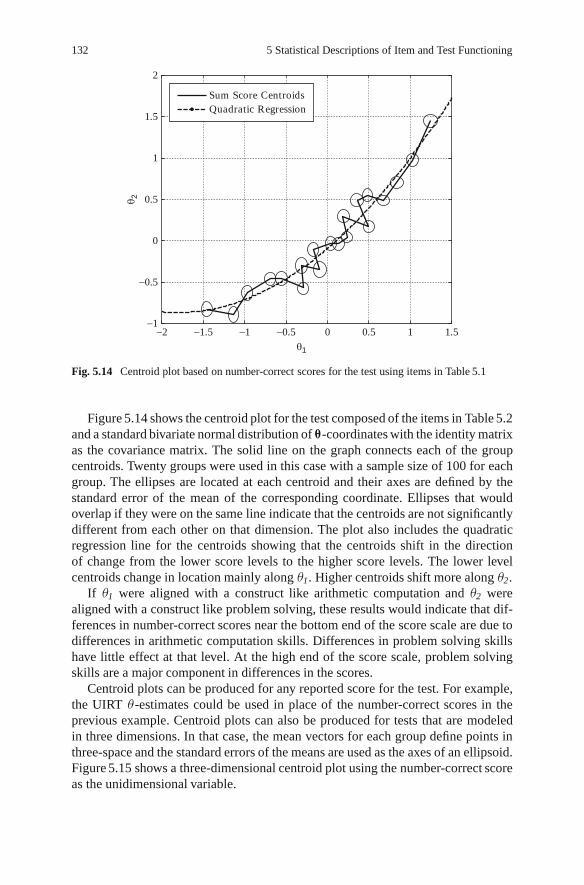
132 5 Statistical Descriptions of Item and Test Functioning
−2 −1.5 −1 −0.5 0 0.5 1 1.5−1
−0.5
0
0.5
1
1.5
2
θ1
θ 2
Sum Score CentroidsQuadratic Regression
Fig. 5.14 Centroid plot based on number-correct scores for the test using items in Table 5.1
Figure 5.14 shows the centroid plot for the test composed of the items in Table 5.2and a standard bivariate normal distribution of ™-coordinates with the identity matrixas the covariance matrix. The solid line on the graph connects each of the groupcentroids. Twenty groups were used in this case with a sample size of 100 for eachgroup. The ellipses are located at each centroid and their axes are defined by thestandard error of the mean of the corresponding coordinate. Ellipses that wouldoverlap if they were on the same line indicate that the centroids are not significantlydifferent from each other on that dimension. The plot also includes the quadraticregression line for the centroids showing that the centroids shift in the directionof change from the lower score levels to the higher score levels. The lower levelcentroids change in location mainly along �1. Higher centroids shift more along �2.
If �1 were aligned with a construct like arithmetic computation and �2 werealigned with a construct like problem solving, these results would indicate that dif-ferences in number-correct scores near the bottom end of the score scale are due todifferences in arithmetic computation skills. Differences in problem solving skillshave little effect at that level. At the high end of the score scale, problem solvingskills are a major component in differences in the scores.
Centroid plots can be produced for any reported score for the test. For example,the UIRT �-estimates could be used in place of the number-correct scores in theprevious example. Centroid plots can also be produced for tests that are modeledin three dimensions. In that case, the mean vectors for each group define points inthree-space and the standard errors of the means are used as the axes of an ellipsoid.Figure 5.15 shows a three-dimensional centroid plot using the number-correct scoreas the unidimensional variable.

5.4 Summary and Conclusions 133
Fig. 5.15 Three-dimensional centroid plot with standard error of the mean ellipsoids and projec-tions onto � -planes
The plot in Fig. 5.15 is based on an analysis of 4,000 cases divided into 40groups of 100 using the number-correct score for the test. The test is composedof 70 dichotomously-scored test items. The error ellipsoids for each centroid arefairly small indicating that the successive centroids are usually significantly differ-ent from each other. The plot also contains the projections of the lines connectingthe centroids onto the side panels of the plot – the planes formed by pairs of �s.The projection onto the �2, �3 plane is close to linear while the projections onto theother planes are nonlinear. A two-dimensional analysis of this test based on �2 and�3 would indicate that the meaning of the differences on the number-correct scorescale is the same over the range of the scale, but the full analysis of the data indi-cate that the meaning of differences on the number-correct score scale change withthe level of performance on the scale.
5.4 Summary and Conclusions
This chapter provides ways for representing the characteristics of test items and testswhen MIRT models are used to describe the interaction between persons and testitems. Some of the statistical indices and graphical representations show the usualIRT item characteristics of difficulty and discrimination. Because MIRT modelsconsider the functioning of items in a multidimensional space, there is also a need toindicate the direction in the space that the item provides the best discrimination. Thisis done by representing an item as an arrow or vector in the multidimensional space.

134 5 Statistical Descriptions of Item and Test Functioning
This type of representation shows the direction of greatest discrimination and helpsshow the relationships among items and the connection between unidimensional andmultidimensional models.
The chapter also presents methods for describing the information provided byitems and tests that can be used for estimating the location of a person in the ™-space.The information about a person’s location in the space is shown to differ by thedirection taken from that location. Items and tests are not equally good at differen-tiating individuals that differ from each other along different coordinate axes. Theconcept of information will prove useful in later chapters when test design issuesare considered.
Finally, the chapter describes the relationship between unidimensional estimatesof a construct and multidimensional representations. The results from unidimen-sional IRT models are shown to be weighted combinations of the estimated co-ordinates from the MIRT solution. The weights are related to the discriminationparameters for the items. Centroid plots are used to show that the meaning ofreported scores may be different at different points along the score scale. Thesemultidimensional representations were designed to help develop greater conceptualunderstanding of the way MIRT models represent test items and clarify the meaningof the results of the application of unidimensional models to multidimensional data.
5.5 Exercises
1. A set of test items require three coordinate axes to represent the interaction be-tween the examinees and the test items. The parameters for two of the test items areprovided in the following table.
Item number a1 a2 a3 d
1 1.2 .5 .4 �12 .35 .9 .9 1
For each item, compute the distance from the origin of the space to the point ofsteepest slope in the space. Which of the two items would be easier for a populationof examinees who are distributed as a standard bivariate normal distribution with� D 0‹ What is the distance along the coordinate axes from the origin of the spaceto the point of steepest slope in that direction? Determine that distance for each itemalong each coordinate axes.
2. A person is located at a distance of 2 units from the origin of a three-dimensionalspace along a line with the following angles with each of the coordinate axes:Œ33:2 63:4 71:6. The angles are in degrees with axes �1, �2, and �3, respectively,and the person has positive coordinates on each axis. Give the person’s location asa 1 �m vector of ™ coordinates.

5.5 Exercises 135
3. Draw the arrow representation for the two items described by the parameters inExercise 1.
4. Figure 5.14 is a centroid plot for the scores from a test that shows differencesmostly along �1 for low scoring examinees and differences with more of a �2 com-ponent for high scoring examinees. Describe how you would select items for a testusing the items’ MIRT parameters so that both low and high scores show differencesalong �2 and mid-range scores show differences along �1. Give your reasons for theapproach to selecting test items.

Chapter 6Estimation of Item and Person Parameters
The MIRT models presented in this book are useful from a theoretical perspectivebecause they provide a model for the interaction between persons and test items. Thedifferent kinds of models represent different theoretical perspectives. For example,the compensatory and partially compensatory models provide two different concep-tions of how levels on hypothetical constructs combine when applied to items thatrequire some level on the constructs to determine the correct response. Althoughthe theoretical models are interesting in their own right, the practical applicationsof the models require a means of estimating the item and person parameters for themodels. Without practical procedures for parameter estimation, the usefulness of themodels is very limited.
This chapter describes the procedures that are currently used for estimatingthe item and person parameters for the models. These procedures are necessarilyembedded within computer programs for carrying out the steps in the estimationmethodology. It is difficult to separate the estimation procedures from the pro-grams used to implement them. An excellent estimation methodology may performpoorly because it is improperly programmed or programmed in an inefficient way.A method with poorer theoretical properties may perform better overall because theprogramming of the method was done in a more creative way. Because of this closetie between estimation methodology and the computer programs used to implementthem, they will be described together in the later sections of this chapter. Beforegetting into the details of estimation procedures, a general overview is provided.This overview is designed to give a conceptual framework for understanding theestimation procedures without getting into the technical details.
This chapter is reasonably up to date about programs and methods as of 2008.However, computer software becomes obsolete and computer systems change fairlyrapidly. For that reason, this chapter does not go into the details of running specificprograms. Those may change by the time this book is published. Rather, the basicestimation model is described for commonly used programs and differences in con-straints used in estimation procedures are presented. These are the features of theestimation methods and programs that explain why different programs applied tothe same item response data give different parameter estimates. Chapter 7 describessome methods for determining if the parameter estimates from different programsare simple transformations of each other.
M.D. Reckase, Multidimensional Item Response Theory, Statistics for Socialand Behavioral Sciences, DOI 10.1007/978-0-387-89976-3 6,c� Springer Science+Business Media, LLC 2009
137

138 6 Estimation of Item and Person Parameters
6.1 Background Concepts for Parameter Estimation
The estimation of the values of parameters for MIRT models is challenging fora number of reasons. First, the models contain parameters for both persons andtest items and generally it is not possible to estimate the two sets of parametersindependent of each other. The consequences of the need to jointly estimate person-and item-parameters are shown in the next section of this chapter. A second reasonthat the estimation of parameters is challenging is that many parameters need to beestimated. For the compensatory model described in Chap. 4, if m is the numberof coordinate axes, n is the number of test items, and N is the number of people,then there are n .mC 1/ C m � N parameters to be estimated. For a 50 item testmodeled with four dimensions calibrated with 2,000 examinees, 8,250 parametersneed to be estimated using 100,000 item responses. A third reason the estimation ischallenging is that there are indeterminacies in the models such as the location ofthe origin of the space, the units of measurement for each coordinate axis, and theorientation of the coordinate axes relative to the locations of the persons. All of theseissues must be addressed in the construction of a computer program for estimatingthe parameters.
The next sections of this chapter describe the parameter estimation process asseparate pieces – the estimation of person locations with item parameters known,and the estimation of item parameters with person locations known – to high-light the general methods that are used and the problems that must be addressedwhen the methods are combined. Following those preliminary descriptions of esti-mation procedures, the methods used in commonly available estimation programswill be described. There is no attempt to give a formal mathematical descriptionof statistical estimation procedures because that would double the length of thisbook. Interested individuals should look at texts such as Baker and Kim (2004) andGamerman and Lopes (2006) for a more complete exposition of statistical estima-tion procedures.
6.1.1 Estimation of the ™-vector with Item Parameters Known
Suppose that there is a large set of test items available that have already been ana-lyzed with a high quality computer program for estimating their parameters. Theseitems have parameter estimates that are based on a large, appropriate sample of ex-aminees. Initially, the item parameters for these items are assumed known withouterror (the estimation error is assumed to be very small) and the problem of estimat-ing the location of examinees with these items is addressed.
Suppose further that an examinee has been selected and the test items are ad-ministered to this person to estimate his or her location in the ™-space. The resultsfrom the administration are the scored responses to the test items. The informationavailable for estimating the location of the examinee is the string of item scores andthe item parameters for the items that have been administered. When computing a

6.1 Background Concepts for Parameter Estimation 139
location estimate, consideration must first be given to the characteristics of a goodestimate. These characteristics provide criteria for choosing one estimate of locationover another. Three different criteria are considered here – the maximum likelihoodcriterion, the maximum a posteriori Bayesian criterion, and the least squares cri-terion. Estimation of an examinee’s location is first described using the maximumlikelihood criterion and then estimation procedures using the other two criteria aredescribed and compared to maximum likelihood procedure.
The maximum likelihood criterion is basically that the estimate of the examinee’slocation is the ™-vector that results in the highest probability for the observed stringof item scores. The term likelihood is used for the probability of the string of itemscores for any candidate value of the ™-vector. The particular ™-vector that yieldsa likelihood for the response string that is higher than all other ™-vectors is themaximum likelihood estimate for the given set of items and the observed stringof item scores. A few examples are provided to show how maximum likelihoodestimation works in practice and to identify some problems with the methodology.The examples begin with the simple two-dimensional case with the compensatorymodel so that graphic representations of the likelihoods of the item score string canbe used. Later examples consider higher dimensional cases.
The first item presented to an examinee has item parameters for the compen-satory model given in (4.5) of a11 D :8, a12 D :5, and d1 D �:6 and the examineeanswers the item correctly so the item score u1 D 1. Figure 6.1 shows the item re-sponse surface for this item as an equi-probable contour plot. In this case, the plotis shaded from black for low probabilities to white for probabilities near 1.0 so thatthe region of highest probability is easy to identify. For the one item case, the item
θ1
θ 2
−4 −3 −2 −1 0 1 2 3 4−4
−3
−2
−1
0
1
2
3
4
0.1
0.2
0.3
0.4
0.5
0.6
0.7
0.8
0.9
Fig. 6.1 Likelihood surface for a correct response to the one item test with a11 D :8, a12 D :5, andd1 D �:5. The bar at the right indicates the relationship between shade of gray and probability

140 6 Estimation of Item and Person Parameters
response surface is the same as the surface showing the likelihoods for the responsestring because it shows the probability of the single item score for various locationsin the ™-space.
Study of the plot shows that the highest probabilities for a correct response occurin the upper right corner where the graph is white. In fact, the probability of a correctresponse is highest at .4; 4/ for the region of the ™-space included on this plot. Theprobability there is .99 and is higher than at any other ™ location shown in the plot.If the surface were not constrained to the region between �4 and 4 on each axis, themaximum would be at .1; 1/ because the surface is monotonically increasing.The undefined point, .1; 1/, is the maximum likelihood estimator of the locationfor the person based on the one item test and a correct response to the test item.
This result is inconvenient because infinite proficiency on the skills required torespond to the test item is difficult to justify as a reasonable estimate. However, itis consistent with the maximum likelihood criterion because a person with infiniteability would be able to answer the item correctly with certainty and no other lo-cation would give that high a probability. This result also emphasizes that one itemtests do not do a very good job of locating a person in a multidimensional ™-space.
The second item presented to an examinee is more difficult with parametersa21 D :2, a22 D 1:1, and d2 D � 1:2 and the examinee responds incorrectly to theitem. The item score vector is now Œ1 0. The likelihood of this response string isgiven by the product of the probability of a correct response to Item 1 and the prob-ability of an incorrect response to Item 2. In general, the likelihood for a responsestring for a particular location in the ™-space is given by the following equation:
L�Uj j ™j
DnY
iD1P�uij j ™j
uijQ�uij j ™j
1�uij; (6.1)
where L�Uj j™j
is the likelihood of response string Uj for a person j located at
™j , and uij is the item score on item i for person j on the n-item test. The othersymbols have been previously defined.
The likelihood surface for this two-item test with the response string 10 is shownin Figure 6.2. This plot shows that the likelihood for the 10 response string is greatestin value at approximately .4; �2/ for the region of the ™-space covered by the plot.At that point, the likelihood is approximately .77, the product of .83 for the proba-bility of a correct response to the first item and .93, the probability of an incorrectresponse to the second item for an examinee at that location. All other ™-values inthis region have lower likelihood values. If the entire ™-space is unlimited, then thelocation of the maximum likelihood value would be at .1; �1/ because infinitelylow proficiency on the second dimension of the space would predict an incorrectresponse to the second item with certainty. The likelihood of the response string 10at this undefined point in the space is 1.
After two responses, the maximum likelihood estimate of the examinees locationis still not very meaningful. The concept of infinitely low proficiency is difficultto comprehend. A two-item test is not very useful for locating an examinee in atwo-dimensional ™-space.

6.1 Background Concepts for Parameter Estimation 141
0.1
0.2
0.3
0.4
0.5
0.6
0.7
θ1
θ 2
−4 −3 −2 −1 0 1 2 3 4−4
−3
−2
−1
0
1
2
3
4
Fig. 6.2 Likelihood surface for a two-item test with response string 10. The bar at the right indi-cates the relationship between the shade of gray and the likelihood at each ™-point
0.05
0.1
0.15
0.2
0.25
θ1
θ 2
−4 −3 −2 −1 0 1 2 3 4−4
−3
−2
−1
0
1
2
3
4
Fig. 6.3 Likelihood surface for the response string 100
The third item presented to an examinee has parameters a31 D 1:0, a32 D :2, andd3 D �2. The examinee answers this test item incorrectly so the resulting responsestring is 100. The likelihood surface for this response string is given in Figure 6.3.For the three-item test with the specified item parameters and the observed itemscores, there is now a location for the maximum of the likelihood function withfinite values for both coordinates. That location is at approximately .1:5; �:75/ in

142 6 Estimation of Item and Person Parameters
the ™-space. The likelihood value at that point is .3101 and it is larger than any otherlikelihood value. However, its magnitude is less than the maximum likelihood forthe two-item case. With each additional item, the magnitude of the maximum ofthe likelihood is smaller because another probability term is added to the product in(6.1). As the number of items in the test increases, the value of the likelihood at themaximum gets very small. For example, if the probability of the observed responsefor each item on a 40 item test were .8, the likelihood of that response pattern wouldbe .840 D :000133, a very small number. To avoid problems that result from workingwith very small numbers, estimation programs often search for the maximum of thelog of the likelihood rather than the likelihood. The log likelihood surface has itsmaximum at the same location as the likelihood surface.
When unidimensional item response theory models are used, finite estimates ofthe person parameters are usually found when item scores of both 0 and 1 are presentin the response string. The exception is for some unusual response strings for thethree-parameter logistic model where the lower asymptote to the model yields max-imums at �1 even when there are both correct and incorrect responses. This resultgenerally indicates that the examinee has been answering questions correctly at lessthan that specified by the lower asymptote parameter. In most cases, however, thepresence of both a correct and incorrect response results in a finite estimate for theperson parameter.
In the example given here, it is clear that having both a correct and incorrectresponse was not sufficient to guarantee that the location of the maximum likeli-hood point would have finite values for all coordinates. This raises questions of theconditions under which the maximum likelihood estimation procedure yields finiteestimates of coordinates for MIRT models. To give some insight into this question,the .5 contour lines are plotted for each of the items used in the example. Thesecontour lines are shown in Figure 6.4. For each line, an arrow shows the direction ofincreasing probability for the item score obtained from the examinee. The responseto the first item was correct, so the arrow points in the increasing direction for both�s from the solid line that is the .5-contour for that item. The other two-item scoreswere 0, so the arrows for those items (dashed and dotted contour lines) are pointingin the negative direction for both �s. The lines and the associated directions of in-creasing slope contain an area in the ™-space that forms a triangle. The maximum ofthe likelihood surface is enclosed within that triangle. Interestingly, the only otherpattern that gives a finite location for the maximum of the likelihood function isobtained by taking the response string 100 and changing all of the ones to zeros andzeros to ones – 011. There are no other response strings that yield locations for themaximum of the likelihood function that have finite coordinates.
The use of the .5-contour lines in this way suggests that there are many caseswhen the likelihood function will not have a useful maximum value. Suppose forexample, four test items all have the same a-parameter vector of Œ1:2 :8, but haved -parameters of �2, �1, 0, 2. The .5-contours for these items will form a parallelset of lines in the ™-space – it is not possible to enclose a space with the lines. If anexaminee answers the two easier items correctly and the two hard items incorrectly,the likelihood surface for that response string is given in Figure 6.5. This surface has
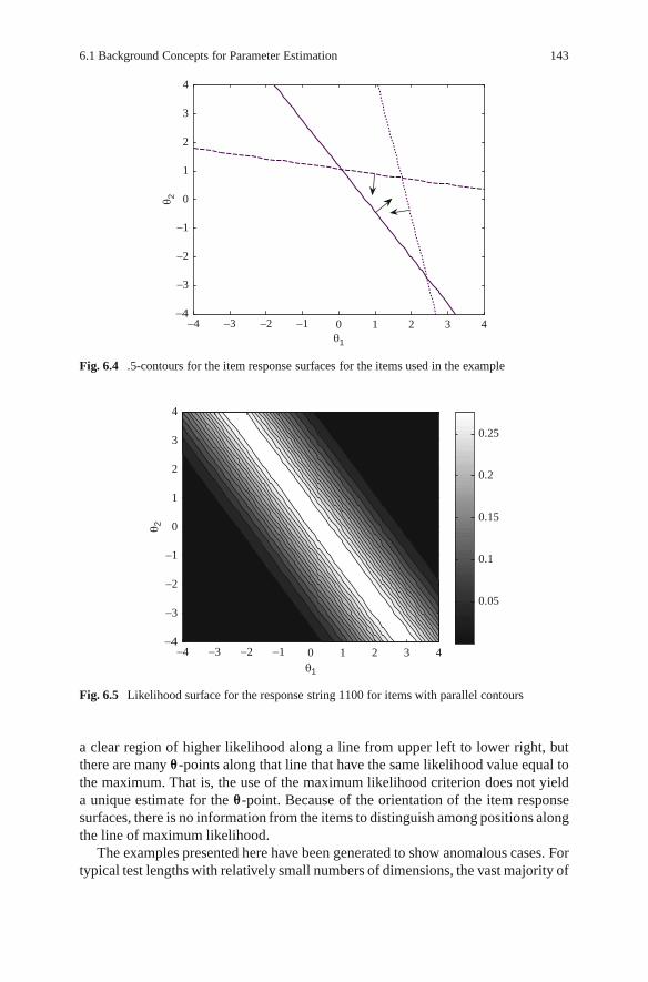
6.1 Background Concepts for Parameter Estimation 143
θ1
θ 2
−4 −3 −2 −1 0 1 2 3 4−4
−3
−2
−1
0
1
2
3
4
Fig. 6.4 .5-contours for the item response surfaces for the items used in the example
0.05
0.1
0.15
0.2
0.25
θ1
θ 2
−4 −3 −2 −1 0 1 2 3 4−4
−3
−2
−1
0
1
2
3
4
Fig. 6.5 Likelihood surface for the response string 1100 for items with parallel contours
a clear region of higher likelihood along a line from upper left to lower right, butthere are many ™-points along that line that have the same likelihood value equal tothe maximum. That is, the use of the maximum likelihood criterion does not yielda unique estimate for the ™-point. Because of the orientation of the item responsesurfaces, there is no information from the items to distinguish among positions alongthe line of maximum likelihood.
The examples presented here have been generated to show anomalous cases. Fortypical test lengths with relatively small numbers of dimensions, the vast majority of

144 6 Estimation of Item and Person Parameters
response strings will yield maximum likelihood estimates that have finite estimatesfor the ™-vector. When maximum likelihood estimation does not yield finite esti-mates, it is usually a symptom that the test was not well designed to determine thelocation in the multidimensional space of the examinee in question. It may have beentoo easy or difficult, or not have enough test items that are sensitive to differencesalong one of the coordinate axes.
When maximum likelihood estimates yield values that are infinite, the pragmaticsolution is to assign values that are as extreme as those that are typically observedin practice. These might be coordinate values such as 4 or �4. This suggests thatthe researcher has other information that indicates that it is not believable to have anestimate of �50 or 100 on a scale with a mean 0 and standard deviation of 1. Thebeliefs of the researcher can be taken into account in a more formal way by usingBayesian estimation procedures.
Bayesian estimation is based on a theorem about the relationship among certainconditional probabilities that was published in 1763 (Bayes 1763). Originally, thetheorem dealt with the probabilities of discrete events. Using modernized notation,Bayes’ Theorem is given by (Stigler 1986, p. 103)
P.Ai jE/ D P.E jAi/P.Ai /P
j
P.E jAj /P.Aj / ; (6.2)
where E is an observed event and Ai is a possible cause for the event. The sum-mation is over all of the possible causes for the event. The denominator of theexpression on the right is the sum of all of the possible numerators. Dividing by thatterm ensures that the terms on the left side of the expression will sum to 1.0 as is req-uired for probabilities. The term P.Ai / is called the prior probability for the causeand the full set of those probabilities form the prior distribution for the cause of theeventE. The termP.Ai jE/ is called the posterior probability of the cause given thatthe event occurred. The full set of these probabilities forms the posterior distributionof the causes of E.
Bayes’ theorem gives the probability that each possible cause is the cause forthe event given the probability of the event if the cause is the correct one, and theprobability of observing a particular cause. In the context of IRT, the event is theobserved string of item scores and the possible causes are the possible values of � .If the possible values of � were discrete points, (6.2) could be used for Bayesianestimation of the ™-vector. A criterion for selecting the best estimate of the ™-vectoris the one that has the highest probability given the observed string of item scores.This estimation criterion is analogous to the maximum likelihood criterion usedwith (6.1).
Because ™ is usually considered to be a continuous rather than a discrete variable,a different version of Bayes’ theorem is used for estimation of the ™-vectors. Thiscontinuous version of Bayes’ theorem is given in many statistics texts (e.g., Degroot1970, p. 28). It is presented here using the same notation used when describingmaximum likelihood estimation.

6.1 Background Concepts for Parameter Estimation 145
h.™ j Uj / D L.Uj j ™/f .™/R
�
L.Uj j ™/f .™/d™; (6.3)
where f .™/ is the prior probability density function for ™, Uj is the item scorestring for Examinee j , L
�Uj j™ is the probability of the item score string given � ,
and h�™jUj
is the posterior probability density of ™ given the item scores string.
Note that the probability of the item score string given ™ is the same as the likeli-hood of the item score string given in (6.1).
Because the denominator of the right side of (6.3) is the same for all values of � ,Bayes’ theorem is sometimes written as
h�™jUj
/ L�Uj j™f .™/ : (6.4)
This form of the theorem indicates that the posterior probability of ™ is proportionalto the likelihood times the prior distribution. The implication is that finding themaximum of the right side of the expression will also yield the maximum of the leftside of the expression.
Bayesian estimation procedures can use a number of different statistics to esti-mate ™. Those used most frequently are the mode and mean of h
�™jUj
. Using
the mode is called maximum a posteriori estimation, or MAP. Using the mean iscalled expected a posteriori estimation, or EAP. If the posterior distribution of ™ issymmetric, these two types of estimates of ™ will yield the same value.
When using Bayesian estimation, the prior distribution of ™ needs to be speci-fied. The form of this distribution may be specified based on previous analyses oftest data or from general knowledge about the form of distributions typically foundin educational or psychological settings. The form of this distribution is requiredbefore the estimation of ™, hence the name given to it is the prior distribution.
When there is little empirical information about the form of the distribution of™-points, the standard multivariate normal distribution with an identity matrix forthe variance/covariance matrix is often used as the prior distribution for Bayesiananalyses. This selection is supported by years of successful use of the multivariatenormal distribution as a default distributional assumption for the analysis of educa-tional and psychological data.
To show the difference between Bayesian and maximum likelihood estimation,the same item score strings that have been used earlier are used to estimate ™ usingthe bivariate normal prior with a zero mean vector and an identity matrix for avariance/covariance matrix. Also, MAP estimation is used. After one item with acorrect response, the equi-density plot for the prior and posterior distributions arepresented in Fig. 6.6.
The plot shows that the posterior distribution of ™ has shifted to the upper rightrelative to the prior distribution. The maximum point on the prior distribution wasat .0; 0/ in the ™-space. After the correct response to one item, the maximum of theposterior distribution is approximately .:5; :25/. This is the MAP estimate of ™ afterthe response to the single item. In contrast to the maximum likelihood estimate that

146 6 Estimation of Item and Person Parameters
θ1
θ 2
−4 −3 −2 −1 0 1 2 3 4−4
−3
−2
−1
0
1
2
3
4
Fig. 6.6 Prior (dotted lines) and posterior (solid lines) probability density functions for a bivariatenormal prior density and a correct response to an item with parameters with a11 D :8, a12 D :5, andd1 D � :5
had maximums approaching infinite values for the � elements, the Bayesian esti-mate has finite coordinates. This is usually seen as a major advantage for Bayesianestimation.
The Bayesian estimate for the item score string of 100, using the same items asfor the maximum likelihood procedure shown in Fig. 6.3, is obtained from the pos-terior density shown in Fig. 6.7. The highest point for the posterior density functionfor this item score string is located at .:25; 0/, a location that is quite different thanthat for the maximum of the likelihood function for the same item score string –.1:5;�:75/. The reason for this large difference is that the bivariate normal priordistribution dominates the posterior distribution when the number of test items issmall. As the number of test items increases, the maximum likelihood estimate andthe MAP estimate become closer to each other.
The fact that the Bayesian estimate is closer to the location of the mean vectorfor the prior distribution than is the maximum likelihood estimate is known as a re-gression effect. Bayesian estimates are acknowledged to have regression effects thatresult in statistically biased estimates of the ™-vector. When an estimator has statis-tical bias the mean of the estimator is not equal to value of the model parameter. Thestatistical bias in the estimation of the location of the ™-vector is often considered asa reasonable trade off for insuring finite estimates of the elements of the ™-vector.
The maximum likelihood and Bayesian estimation procedures can be used toestimate the item parameters as well as the ™-vectors. For item parameter estimation,the ™-vectors are assumed known and the item parameter space is searched to findthe set of parameters that yields the maximum of the likelihood function or theBayesian posterior distribution. The maximum of the functions cannot be shownhere as points on surfaces because even when there are only two ™-coordinates,

6.1 Background Concepts for Parameter Estimation 147
0.005
0.01
0.015
0.02
0.025
0.03
0.035
θ1
θ 2
−4 −3 −2 −1 0 1 2 3 4−4
−3
−2
−1
0
1
2
3
4
Fig. 6.7 Posterior distribution for the item score string 100
there are three item parameters – a1, a2, and d . The likelihood or the height of theBayesian posterior would need a fourth coordinate axis to show where the height ofthe surface is maximum for a set of item parameters. As a result, graphic methodscannot be used to find the estimates for the item parameters.
The two estimation criteria presented earlier identify the estimate for the ™-vectorby searching for the maximum of the likelihood function of the posterior densitydistribution. It is also possible to specify a criterion for estimation that is based onminimizing the difference between predictions from the MIRT model and the ob-served data. A common predictor for an observation is the expected value of theobservation, in this caseE .u j ™; a; d /. Minimizing the squared difference betweenthe observed value and the predicted value is called the least squares criterion for anestimator. The expected value of the item score is simply P .u D 1j ™; a; d /, so aleast squares method for finding the estimate of ™ is to find the vector ™ that resultsin a minimum value for the following expression.
SS� DnX
iD1.ui � P .ui D 1 j ™; ai ; di //
2 ; (6.5)
where SS� is the sum of squared differences for a particular value of ™, and ui is the0 or 1 item score for Item i .
The sum of squared differences can be computed for each ™-point. The ™-pointthat yields the smallest value for SS� is the least squares estimator for ™. The sum-of-squares surface for the item score string 100 is presented in Fig. 6.8. In contrast toFigs. 6.3 and 6.7, the estimator is given by the low point for this surface rather thanthe high point. In this case, the least squares estimate of ™ is .1:5;�:5/, a point closeto the maximum likelihood estimator .1:5;�:75/. Least squares estimators based

148 6 Estimation of Item and Person Parameters
0.4
0.6
0.8
1.2
1
1.4
1.6
θ1
θ 2
−4 −3 −2 −1 0 1 2 3 4−4
−3
−2
−1
0
1
2
3
4
Fig. 6.8 Least squares surface for the item score string 100
on (6.5) are not often used for the estimation of MIRT parameters, but variationson this approach are used in the NOHARM estimation program. The details of thatleast-squares approach are given later in the chapter.
All of the estimation procedures described earlier select a criterion and thensearch for the parameter vector that best satisfies the criterion. Three criteria weredescribed: (a) maximum likelihood, (b) Bayesian maximum a posteriori, and (c)least squares. These are not the only criteria that can be used. For example, as wasnoted earlier, the mean vector for the posterior distribution can be used instead ofthe vector of maximum values. The former estimation criterion is called expected aposteriori. Other estimation criteria are available as well.
When these approaches are used in practice, graphic procedures for finding theparameter vector are not used. Instead, mathematical search procedures for the max-imum or minimum of a function are used. The details of these search procedures areprovided in the next section of this chapter.
6.2 Computer Programs for Estimating MIRT Parameters
A number of computer programs have been developed for estimating the valuesof the parameters in MIRT models. The programs use a variety of estimation proce-dures and sometimes they include more than one option. A sampling of the computerprograms that are available are described here. It is not possible to provide a com-plete list of computer programs or even to accurately describe the procedures in anyone computer program. Computer methodology changes very rapidly and the infor-mation presented here may be dated by the time this book is published. Also, newand better computer programs may become available. For all of these reasons, the

6.2 Computer Programs for Estimating MIRT Parameters 149
inclusion of a computer program here is not an endorsement. Rather, the computerprogram is used as a practical example of the ways that estimation procedures areimplemented in practice. Those who wish to estimate the values of the parametersof MIRT models should review the current literature to determine the best of thecurrently available programs.
6.2.1 TESTFACT
TESTFACT (Bock, Gibons, Schilling, Muraki, Wilson, and Wood 2003) is a com-puter program for performing factor analysis of interitem tetrachoric correlationsand what the authors label “modern methods of item factor analysis based on itemresponse theory.” The modern methods of item factor analysis include the estima-tion of the item and person parameters for the multidimensional extension of thetwo-parameter normal ogive model. The user can also input lower asymptote pa-rameters so that the program can use the multidimensional generalization of thethree-parameter normal ogive model. The program does not estimate the lowerasymptote parameter for the items.
The program estimates the MIRT model item parameters using a variation ofthe maximum likelihood method called marginal maximum likelihood (Bock andAitken 1981). Estimates of the ™-vectors are obtained using a Bayesian estimationmethod. The method of estimation is described in some detail in Bock, Gibbons, andMuraki (1988). That method is briefly described here. Some recent enhancementsare described in Bock and Schilling (2003).
The estimation of the item parameters is based on the likelihood of an item scorestring given in (6.1). That likelihood is used to specify the probability of observ-ing the item score string in the population of examinees. This overall probabilityof the item score string is obtained by weighting the likelihood by the probabilitydensity of the ™-vectors and then integrating over the ™-space. The equation for theprobability of the score response string for the population of examinees is given by
P .u D u`/ DZ
™
L.u` j ™/ g .™/ d™; (6.6)
where P .u D u`/ is the probability of item score string u` for the populationof examinees,L.u`j™/ is the likelihood of the item score string given a particular™-vector (see (6.1)), and g .™/ is the probability density function for ™.
The integral in (6.6) is evaluated through an integral approximation procedure.When the number of dimensions is five or less, Gauss–Hermite quadrature is used
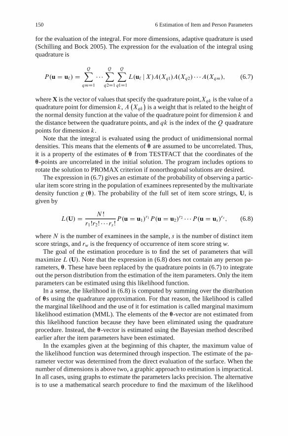
150 6 Estimation of Item and Person Parameters
for the evaluation of the integral. For more dimensions, adaptive quadrature is used(Schilling and Bock 2005). The expression for the evaluation of the integral usingquadrature is
P.u D u`/ DQX
qmD1� � �
QX
q2D1
QX
q1D1L.u` jX/A.Xq1/A.Xq2/ � � �A.Xqm/; (6.7)
where X is the vector of values that specify the quadrature point,Xqk is the value of aquadrature point for dimension k, A
�Xqk
is a weight that is related to the height of
the normal density function at the value of the quadrature point for dimension k andthe distance between the quadrature points, and qk is the index of theQ quadraturepoints for dimension k.
Note that the integral is evaluated using the product of unidimensional normaldensities. This means that the elements of ™ are assumed to be uncorrelated. Thus,it is a property of the estimates of ™ from TESTFACT that the coordinates of the™-points are uncorrelated in the initial solution. The program includes options torotate the solution to PROMAX criterion if nonorthogonal solutions are desired.
The expression in (6.7) gives an estimate of the probability of observing a partic-ular item score string in the population of examinees represented by the multivariatedensity function g .™/. The probability of the full set of item score strings, U, isgiven by
L.U/ D NŠ
r1Šr2Š � � � rsŠP.u D u1/r1P.u D u2/r2 � � �P.u D us/rs ; (6.8)
where N is the number of examinees in the sample, s is the number of distinct itemscore strings, and rw is the frequency of occurrence of item score string w.
The goal of the estimation procedure is to find the set of parameters that willmaximize L.U/. Note that the expression in (6.8) does not contain any person pa-rameters, ™. These have been replaced by the quadrature points in (6.7) to integrateout the person distribution from the estimation of the item parameters. Only the itemparameters can be estimated using this likelihood function.
In a sense, the likelihood in (6.8) is computed by summing over the distributionof ™s using the quadrature approximation. For that reason, the likelihood is calledthe marginal likelihood and the use of it for estimation is called marginal maximumlikelihood estimation (MML). The elements of the ™-vector are not estimated fromthis likelihood function because they have been eliminated using the quadratureprocedure. Instead, the ™-vector is estimated using the Bayesian method describedearlier after the item parameters have been estimated.
In the examples given at the beginning of this chapter, the maximum value ofthe likelihood function was determined through inspection. The estimate of the pa-rameter vector was determined from the direct evaluation of the surface. When thenumber of dimensions is above two, a graphic approach to estimation is impractical.In all cases, using graphs to estimate the parameters lacks precision. The alternativeis to use a mathematical search procedure to find the maximum of the likelihood

6.2 Computer Programs for Estimating MIRT Parameters 151
function. TESTFACT uses a procedure based on expectation/maximization (EM)algorithm developed by Dempster, Laird, and Rubin (1977).
The estimation procedure in TESTFACT is based on the common mathematicalnotion that the maximum of a surface is the place where the tangent plane to the sur-face has slope of zero in all directions. The point where the tangent plane touches thesurface is the maximum of the surface. This is the place where the partial derivativesof the surface with respect to the parameters of interest are zero. Bock, Gibbons, andMuraki (1988) give a general expression for the derivative of the likelihood func-tion given in (6.8). The expression uses v to represent one of the item parameters,the elements of the a-vector or the d parameter. Using the notation from (6.8), theexpression for the derivative is given in (6.9).
@ logL.U/@vi
DsX
`D1
r`
P.u D u`/
�@P.u D u`/
@vi
�
DZ
™
ri �Nˆi.™/ˆi .™/ Œ1 �ˆi.™/
@ˆj .™/
@vig.™/d™; (6.9)
where
ri DsX
`D1
r`u`iL .u` j ™/
P .u D u`/
is the number of correct responses to item i estimated from the MIRT model andthe estimated item parameters, and
N DX r`L .u` j ™/
P .u D u`/
is the total frequency estimated from the MIRT model and the estimated item pa-rameters. Note that j .™/ is the normal ogive version of the MIRT model. That isthe model used in the TESTFACT program.
The estimation of the number of correct responses using the MIRT model withthe estimated item parameters constitutes the E-step (estimation step) of the EMalgorithm. These estimates are substituted into (6.9) to obtain the maximum likeli-hood estimates of the item parameters in the M-step (maximization step). Becausethe estimates of frequencies depend on estimates of item parameters, the processmust be iterated to get to a solution that gives a close approximation to the observedfrequencies of response patterns.
Equation (6.9) specifies n .mC 1/ nonlinear equations that are simultaneouslyset to 0 and solved. The simultaneous solution of all of these equations requires asubstantial amount of computation and various methods have been used to speed upthe process. Constraints have also been placed on the item parameter estimates tofacilitate convergence. Details of these techniques are provided in Bock, Gibbons,and Muraki (1988) and the TESTFACT manual. The results of the process are esti-mates of the a-parameters (m per item) and the d -parameter (one per item) for each

152 6 Estimation of Item and Person Parameters
of the n items. The solution process is fairly slow. Even with the current generationof fast computers, the solution time is typically in tens of minutes. Of course, by thetime this book is published, the speeds of computers will have increased, reducingthe computing time.
To obtain unique solutions for the item parameters, several indeterminacies inthe MIRT model must be dealt with through constraints. These indeterminacies in-clude the location of the origin of the ™-space, the units of measurement for eachcoordinate axis, and the rotation of the solution relative to the points in the space.The first two indeterminacies are dealt with through the assumption of a multivariatenormal distribution for the ™-vectors with a mean vector containing all 0 elementsand an identity matrix for the variance/covariance matrix. The initial solution forthe model used in TESTFACT deals with the rotational indeterminacy by setting theaik parameters to 0 when k > i . This solution is not presented in the output from theprogram. Instead, the output includes the solution after it is rotated to the principalfactor solution.
Once the item parameters have been estimated, an option is available to estimatethe ™-vectors. The procedure for estimating the ™-vectors is described in Murakiand Englelhard (1985). A Bayesian expected a posteriori (EAP) is used so that es-timates of coordinates from item score string from short tests will not tend towardinfinite values. That is, the estimate of the coordinates in the ™-space for a person isthe expected value of the posterior distribution for each coordinate in � . The basicmathematical expressions for the estimates are
O�j v D E��j v j ui
DZ
™
�vP�™ j uj
d™ D
Z
™
�vf�uj j ™
g .™/
h�uj d™; (6.10)
where O�j v is the estimate of the coordinate on dimension v for person j , f�uj j™
is the likelihood function for the item score string based on the MIRT model, g .™/is the prior distribution for ™, and h
�uj D R
™
f�ujj™
g .™/ d™.
The integral in (6.10) is evaluated using Gauss–Hermite quadrature assumingthat the parameters for the items are known. The standard deviation of the poste-rior distribution is reported as the standard error of measurement for the coordinateestimate.
Two data sets with known characteristics are used here to demonstrate the func-tioning of the estimation procedures. The same data sets are used with all of theprocedures described in this chapter so that they can be directly compared. The itemparameters for the data sets are shown in Table 6.1. A test consisting of 30 dichoto-mously scored test items is assumed to be accurately modeled in a three dimensionalspace using the compensatory logistic model shown in (4.5). The table contains thethree a-parameters for each item and the d -parameter as well as the multidimen-sional discrimination estimate A, the multidimensional difficulty estimate B , andthe angles of the direction of best measurement, ˛v, for each item with the coordi-nate axes for the space.
The set of test items was developed to approximate simple structure in that eachtest best measures along one of the coordinate axes. However, the set of test items

6.2 Computer Programs for Estimating MIRT Parameters 153
Table 6.1 Item parameters and descriptive statistics for 30 test items in three dimensions
Itemnumber
a1 a2 a3 d ˛1 ˛2 ˛3 A B
1 0.7471 0.0250 0.1428 0:1826 11 88 79 0.76 �0:242 0.4595 0.0097 0.0692 �0:1924 9 89 81 0.46 0:41
3 0.8613 0.0067 0.4040 �0:4656 25 90 65 0.95 0:49
4 1.0141 0.0080 0.0470 �0:4336 3 90 87 1.02 0:43
5 0.5521 0.0204 0.1482 �0:4428 15 88 75 0.57 0:77
6 1.3547 0.0064 0.5362 �0:5845 22 90 68 1.46 0:40
7 1.3761 0.0861 0.4676 �1:0403 19 87 71 1.46 0:71
8 0.8525 0.0383 0.2574 0:6431 17 88 73 0.89 �0:729 1.0113 0.0055 0.2024 0:0122 11 90 79 1.03 �0:0110 0.9212 0.0119 0.3044 0:0912 18 89 72 0.97 �0:0911 0.0026 0.2436 0.8036 0:8082 90 73 17 0.84 �0:9612 0.0008 0.1905 1.1945 �0:1867 90 81 9 1.21 0:15
13 0.0575 0.0853 0.7077 0:4533 85 83 8 0.72 �0:6314 0.0182 0.3307 2.1414 �1:8398 90 81 9 2.17 0:85
15 0.0256 0.0478 0.8551 0:4139 88 87 4 0.86 �0:4816 0.0246 0.1496 0.9348 �0:3004 89 81 9 0.95 0:32
17 0.0262 0.2872 1.3561 �0:1824 89 78 12 1.39 0:13
18 0.0038 0.2229 0.8993 0:5125 90 76 14 0.93 �0:5519 0.0039 0.4720 0.7318 1:1342 90 57 33 0.87 �1:3020 0.0068 0.0949 0.6416 0:0230 89 82 8 0.65 �0:0421 0.3073 0.9704 0.0031 0:6172 72 18 90 1.02 �0:6122 0.1819 0.4980 0.0020 �0:1955 70 20 90 0.53 0:37
23 0.4115 1.1136 0.2008 �0:3668 70 22 80 1.20 0:30
24 0.1536 1.7251 0.0345 �1:7590 85 5 89 1.73 1:02
25 0.1530 0.6688 0.0020 �0:2434 77 13 90 0.69 0:35
26 0.2890 1.2419 0.0220 0:4925 77 13 89 1.28 �0:3927 0.1341 1.4882 0.0050 �0:3410 85 5 90 1.49 0:23
28 0.0524 0.4754 0.0012 0:2896 84 6 90 0.48 �0:6129 0.2139 0.4612 0.0063 0:0060 65 25 89 0.51 �0:0130 0.1761 1.1200 0.0870 0:0329 81 10 86 1.14 �0:03
was designed to be fairly realistic in that the angles with the coordinate axes are notall close to 0 or 90ı. The B estimates are in a reasonable range and the A estimatesare not too large.
These item parameters were used to generate data sets with two different vari-ance/covariance matrices for the coordinates for simulated examinees. Data Set1 was generated assuming a mean vector of 0 and an identity matrix for thevariance/covariance matrix. Data Set 2 was designed to represent more realistic con-ditions. The mean vector was set to Œ�:4 � :7:1 and the variance/covariance matrixwas set to
2
41:21 :297 1:232
:297 :81 :252
1:232 :252 1:96
3
5 :

154 6 Estimation of Item and Person Parameters
Table 6.2 Descriptive statis-tics and reliability estimatesfor the number-correct scoresfrom the two simulateddata sets
Data Set 1 Data Set 2
Mean 14:75 12:71
Standard deviation 4:75 6:09
Reliability :71 :84
This matrix is consistent with standard deviations for the coordinates of Œ1:1 :9 1:4and a correlation matrix of 2
41 :3 :8
:3 1 :2
:8 :2 1
3
5 :
The reason for using these values to generate the data is to show the parameterestimates that result when the data do not match the assumptions built into the es-timation program. These assumptions are often a multivariate normal distributionwith mean vector 0 and identity matrix for the variance/covariance matrix.
The analysis data were generated by first randomly selecting 2,000 ™-vectorsfrom each of the two specified population distributions. The two sets of ™-vectorswere then used to generate item score strings using the item parameters shown inTable 6.1. The results were two 2000 � 30 matrixes of item scores. The means,standard deviations, and coefficient ˛ estimates of internal consistency reliability forthe number-correct scores computed from these data sets are presented in Table 6.2.
The differences in the number-correct score distributions and reliabilities for thetwo simulated tests reflect the differences in the ™-distributions used to generatethe data. The ™-distribution for Data Set 1 had means of 0 on the three coordinatesso the mean number-correct score is approximately half of the total possible. Thereliability is moderate because the dimensionality of the generated data violates theassumptions of the internal consistency reliability measure.
Data Set 2 has a lower mean number-correct score because the means for twoof the ™-coordinates are below 0. The standard deviation and reliability are higherbecause the ™-coordinates are correlated resulting in a more internally consistenttest. The differences in the analyses of the two data sets reinforce the sample specificnature of these descriptive statistics. These differences exist because of differencesin the ™-distributions. The same item parameters were used to generate the twodata sets.
The item score matrices from the two data sets were analyzed using TESTFACTspecifying three dimensions using the default options. Item parameter estimates forData Set 1 converged in 14 cycles. The estimation for the item parameters for DataSet 2 did not converge in 200 cycles. The item parameter estimates obtained fromthe two data sets are shown in Table 6.3.
The analysis of Data Set 1 shows that the order of the dimensions in the TEST-FACT output does not match that of the generating data. Dimension 1 of thegenerating parameters corresponds to Dimension 3 from TESTFACT. Dimension 3of the generating parameters corresponds to Dimension 1 for the estimates and Di-mension 2 in the generating parameters remains as Dimension 2 for the estimates.Another feature of the Data Set 1 estimates is that the values of the a-parameters are

6.2 Computer Programs for Estimating MIRT Parameters 155
Table 6.3 Item parameter estimates for Data Set 1 and Data Set 2
Item number Data Set 1 Data Set 2a1 a2 a3 d a1 a2 a3 d
1 .04 .09 .50 :08 .52 .06 :33 �:082 .02 �:00 .27 �:09 .31 .04 :17 �:263 .15 .07 .58 �:29 .64 .14 :31 �:434 �:09 .08 .67 �:29 .46 .22 :33 �:495 .16 .03 .33 �:22 .38 .11 :19 �:366 .16 .10 .67 �:31 1.23 .27 :49 �:737 .20 .16 .89 �:63 .98 .19 :42 �:838 .12 .03 .51 :40 .66 .17 :38 :19
9 .12 .04 .60 :04 .76 .09 :44 �:2210 .06 .05 .54 :05 .71 .11 :30 �:2011 .47 .14 .07 :45 .68 .22 :07 :43
12 .63 .02 .14 �:14 .93 .17 �:11 �:1613 .42 .04 .11 :23 .58 .04 :05 :23
14 1.09 .03 .17 �1:02 1.53 .30 :03 �:9415 .51 .02 .08 :23 .69 .11 �:06 :29
16 .55 .01 .05 �:16 .79 .11 �:02 �:1617 .85 .05 .05 �:16 1.06 .28 �:02 �:1718 .54 .16 .12 :31 .75 .10 �:05 :34
19 .56 .18 .06 :71 .59 .25 :01 :55
20 .39 �:00 .05 :03 .53 .06 �:04 �:0321 .05 .65 .06 :38 .18 .54 :17 �:1722 �:01 .27 .11 �:12 .10 .29 :10 �:3923 .16 .65 .15 �:17 .41 .61 :14 �:7824 .12 1.08 .01 �1:07 .11 .81 :15 �1:6725 .01 .37 .01 �:14 .14 .39 :05 �:4726 .08 .73 .04 :29 .20 .67 :10 �:2627 .06 .91 .06 �:21 .13 .68 �:02 �:8628 .03 .35 �:02 :16 .08 .29 :03 �:1029 .04 .30 .08 :00 .11 .32 :18 �:2430 .11 .65 .05 :06 .26 .54 :05 �:52Note: The largest a-parameter for each item is shown in bold italics.
less than the corresponding generating parameters. This is also true for the estimatesof the d -parameters. This is a result of the fact that the data were generated with thelogistic compensatory MIRT model without the 1.7 constant in the exponent thatimproves the match to the normal ogive model. Because TESTFACT assumes thenormal ogive model, the parameter estimates for a are approximately the generatingvalues divided by 1.7. The actual ratios of the means of the generating a-parametersto the estimated a-parameters are 1.62, 1.59, and 1.88, respectively. The average ofthese three values is 1.7. Also, the ratio of the standard deviations of the generatingd -parameters .:657/ to the estimated d -parameters .:386/ is 1.7.
If the data had been generated with the 1.7 multiplier in the exponent of themodel, the parameter estimates should more closely match the parameters used to

156 6 Estimation of Item and Person Parameters
Table 6.4 Item parameter estimates for Data Set 1a
Item Number a1 a2 a3 d
1 .10 .16 .73 :18
2 .02 .05 .48 �:193 .28 .12 .88 �:484 �:00 .14 .97 �:455 .07 .13 .51 �:416 .29 .11 1.38 �:617 .22 .32 1.21 �1:058 .14 .21 .82 :61
9 .12 .08 .89 :07
10 .22 .13 .82 :12
11 .79 .14 .05 :78
12 1.11 .07 .19 �:1913 .69 .04 .11 :44
14 1.73 .19 .23 �1:6215 .80 �:03 .16 :40
16 .91 .05 .10 �:3217 1.36 .18 .15 �:2118 .84 .12 .15 :54
19 .62 .37 .01 1:06
20 .59 .01 .10 :03
21 .02 .90 .24 :58
22 .02 .48 .18 �:1523 .12 1.15 .28 �:3624 .12 1.41 �:04 �1:5525 .09 .65 .08 �:2726 .10 1.22 .07 :61
27 .12 1.47 �:06 �:3128 �:04 .47 .05 :35
29 .03 .45 .15 �:0130 .15 1.00 .07 :01
Note: The largest a-parameter for each item is shown in bold italics.
generate the data. To demonstrate that situation, a third data set was generated (DataSet 1a) using the item parameters in Table 6.1, the zero vector for means, the identitymatrix as the variance covariance matrix, but with 1.7 in the model. The results ofthe estimation of the item parameters for that data set are given in Table 6.4. Theseresults show a much closer recovery of the generating item parameters than was thecase for Data Set 1. Even though the results appear to be different, they are reallya change of scale. The corresponding parameter estimates from the two data setscorrelate in the high .90s.
The relationships between the parameter estimates from Data Set 2 and the gen-erating item parameters are not as clear as those for Data Sets 1 and 1a. Becausethe coordinates of simulated examinees on Dimensions 1 and 3 were correlated .8when the data were generated, the a-parameters for the 20 items that are sensitive
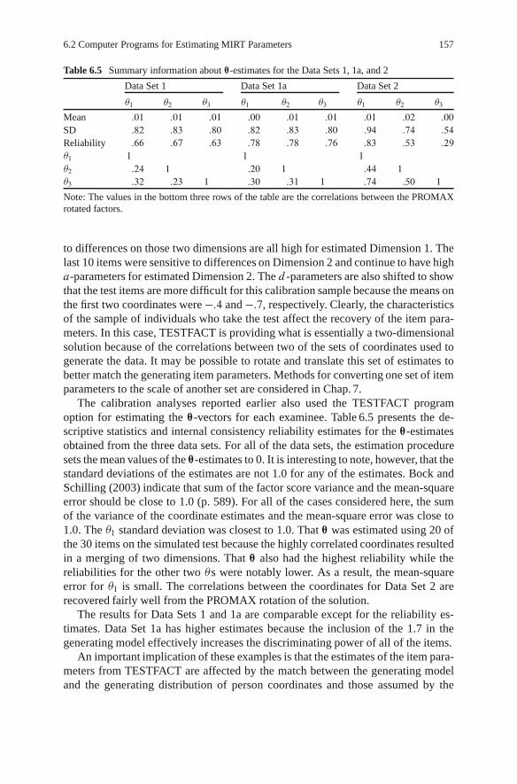
6.2 Computer Programs for Estimating MIRT Parameters 157
Table 6.5 Summary information about ™-estimates for the Data Sets 1, 1a, and 2
Data Set 1 Data Set 1a Data Set 2
�1 �2 �3 �1 �2 �3 �1 �2 �3
Mean :01 :01 :01 :00 :01 :01 :01 :02 :00
SD :82 :83 :80 :82 :83 :80 :94 :74 :54
Reliability :66 :67 :63 :78 :78 :76 :83 :53 :29
�1 1 1 1
�2 :24 1 :20 1 :44 1
�3 :32 :23 1 :30 :31 1 :74 :50 1
Note: The values in the bottom three rows of the table are the correlations between the PROMAXrotated factors.
to differences on those two dimensions are all high for estimated Dimension 1. Thelast 10 items were sensitive to differences on Dimension 2 and continue to have higha-parameters for estimated Dimension 2. The d -parameters are also shifted to showthat the test items are more difficult for this calibration sample because the means onthe first two coordinates were �:4 and �:7, respectively. Clearly, the characteristicsof the sample of individuals who take the test affect the recovery of the item para-meters. In this case, TESTFACT is providing what is essentially a two-dimensionalsolution because of the correlations between two of the sets of coordinates used togenerate the data. It may be possible to rotate and translate this set of estimates tobetter match the generating item parameters. Methods for converting one set of itemparameters to the scale of another set are considered in Chap. 7.
The calibration analyses reported earlier also used the TESTFACT programoption for estimating the ™-vectors for each examinee. Table 6.5 presents the de-scriptive statistics and internal consistency reliability estimates for the ™-estimatesobtained from the three data sets. For all of the data sets, the estimation proceduresets the mean values of the ™-estimates to 0. It is interesting to note, however, that thestandard deviations of the estimates are not 1.0 for any of the estimates. Bock andSchilling (2003) indicate that sum of the factor score variance and the mean-squareerror should be close to 1.0 (p. 589). For all of the cases considered here, the sumof the variance of the coordinate estimates and the mean-square error was close to1.0. The �1 standard deviation was closest to 1.0. That ™ was estimated using 20 ofthe 30 items on the simulated test because the highly correlated coordinates resultedin a merging of two dimensions. That ™ also had the highest reliability while thereliabilities for the other two �s were notably lower. As a result, the mean-squareerror for �1 is small. The correlations between the coordinates for Data Set 2 arerecovered fairly well from the PROMAX rotation of the solution.
The results for Data Sets 1 and 1a are comparable except for the reliability es-timates. Data Set 1a has higher estimates because the inclusion of the 1.7 in thegenerating model effectively increases the discriminating power of all of the items.
An important implication of these examples is that the estimates of the item para-meters from TESTFACT are affected by the match between the generating modeland the generating distribution of person coordinates and those assumed by the
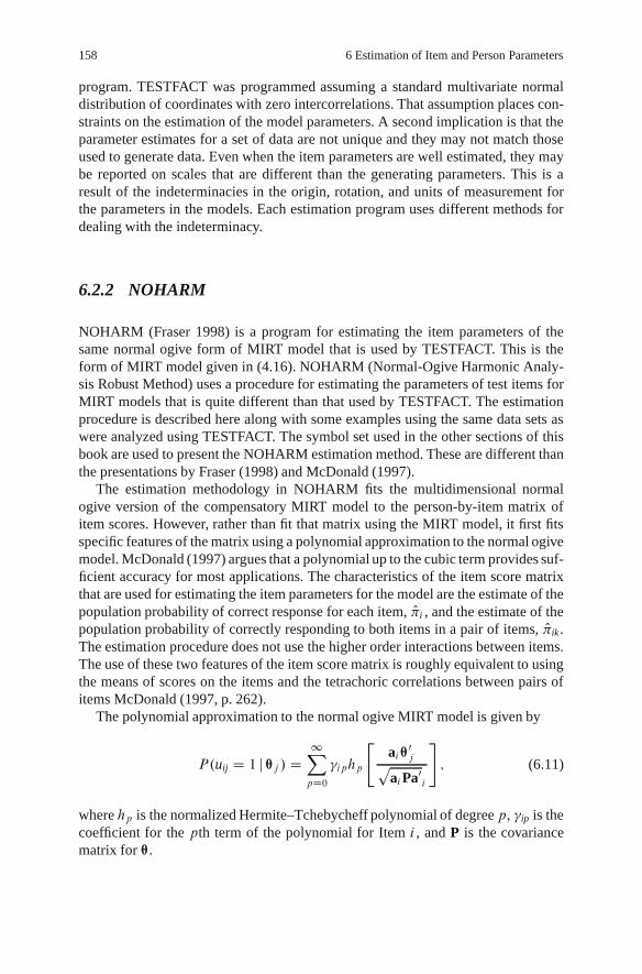
158 6 Estimation of Item and Person Parameters
program. TESTFACT was programmed assuming a standard multivariate normaldistribution of coordinates with zero intercorrelations. That assumption places con-straints on the estimation of the model parameters. A second implication is that theparameter estimates for a set of data are not unique and they may not match thoseused to generate data. Even when the item parameters are well estimated, they maybe reported on scales that are different than the generating parameters. This is aresult of the indeterminacies in the origin, rotation, and units of measurement forthe parameters in the models. Each estimation program uses different methods fordealing with the indeterminacy.
6.2.2 NOHARM
NOHARM (Fraser 1998) is a program for estimating the item parameters of thesame normal ogive form of MIRT model that is used by TESTFACT. This is theform of MIRT model given in (4.16). NOHARM (Normal-Ogive Harmonic Analy-sis Robust Method) uses a procedure for estimating the parameters of test items forMIRT models that is quite different than that used by TESTFACT. The estimationprocedure is described here along with some examples using the same data sets aswere analyzed using TESTFACT. The symbol set used in the other sections of thisbook are used to present the NOHARM estimation method. These are different thanthe presentations by Fraser (1998) and McDonald (1997).
The estimation methodology in NOHARM fits the multidimensional normalogive version of the compensatory MIRT model to the person-by-item matrix ofitem scores. However, rather than fit that matrix using the MIRT model, it first fitsspecific features of the matrix using a polynomial approximation to the normal ogivemodel. McDonald (1997) argues that a polynomial up to the cubic term provides suf-ficient accuracy for most applications. The characteristics of the item score matrixthat are used for estimating the item parameters for the model are the estimate of thepopulation probability of correct response for each item, O�i , and the estimate of thepopulation probability of correctly responding to both items in a pair of items, O�ik.The estimation procedure does not use the higher order interactions between items.The use of these two features of the item score matrix is roughly equivalent to usingthe means of scores on the items and the tetrachoric correlations between pairs ofitems McDonald (1997, p. 262).
The polynomial approximation to the normal ogive MIRT model is given by
P.uij D 1 j ™j / D1X
pD0�iphp
"ai™0
jpaiPa0
i
#
; (6.11)
where hp is the normalized Hermite–Tchebycheff polynomial of degree p, �ip is thecoefficient for the pth term of the polynomial for Item i , and P is the covariancematrix for ™.

6.2 Computer Programs for Estimating MIRT Parameters 159
In practice, only the first four terms of the polynomial are used to estimate theitem parameters. Note that the covariance matrix P is present in (6.11). For the cali-bration of test items, P is usually assumed to be an identity matrix. This assumptionis not a formal part of the MIRT model, but it is used when estimating parameters.NOHARM allows the user to specify other forms for P than the identity matrix.
If, for convenience zj D ai™0j =p
aiPa0i , the form of the first four terms of hp.zj /
are: h0.zj / D 1, h1.zj / D zj , h2.zj / D .z2j �1/=p2, and h3.zj / D .z3j �3zj /=p6.
The estimate of the proportion answering the item correctly is given by the coeffi-cient of the first term of the series. That is,
O�i D �i0 D ˆ
"dip
1C aiPa0i
#
: (6.12)
The estimate of the probability of correctly responding to both test items, i and k,in a pair is given by
O�ik D1X
pD0�ip�jp
"aiPa0
kpaiPa0
iakPa0k
#p: (6.13)
In practice, only the first few terms of the summation are used to approximatethe proportion of correct responses to both items in the i; j -pair (McDonald 1997,p. 261).
The actual estimation of the item parameters is done using unweighted leastsquares methodology. The following criterion (6.14) is minimized relative to theitem parameters,
SSik DX
i¤k.pik � O�ik/
2 for all i; k; (6.14)
where pik is the observed proportion correct for both items in the i; k pair. InNOHARM, the parameters that minimize (6.14) are found using a quasi-Newtonalgorithm.
To demonstrate the results of applying this methodology for the estimation ofitem parameters, NOHARM was run in exploratory mode on the same data-sets thatwere analyzed using TESTFACT. The item parameters used to generate the data aregiven in Table 6.1. Both Data Set 1 and 2 were analyzed to show the results when thedata were generated meeting the assumptions of the estimation program and whenthey were not.
Table 6.6 contains the item parameter estimates for the two data sets. For bothdata sets, some of the a-parameter estimates are set to 0 to fix the orientation of thecoordinate axes. For the examples, a2 and a3 are set to 0 for Item 1 and a3 is set to 0for Item 2. These fixed values are defaults in the program. Fixing these a-parametersin this way sets the �1-axis to align with the direction of maximum discriminationfor Item 1 and the direction of maximum discrimination of Item 2 is set to fallwithin the �1, �2-plane. The directions for the other items are determined from their

160 6 Estimation of Item and Person Parameters
Table 6.6 Item parameter estimates for Data Set 1 and Data Set 2
Item number Data Set 1 Data Set 2
a1 a2 a3 d a1 a2 a3 d
1 .62 .00 .00 :09 1.20 .00 .00 �:092 .25 .04 .00 �:08 .25 .35 .00 �:263 .56 .18 .02 �:28 .54 .34 .35 �:424 .58 .07 �:11 �:27 .32 .29 .39 �:475 .34 .16 .05 �:22 .32 .19 .25 �:356 .63 .20 .01 �:30 .97 .73 .68 �:717 .77 .24 .03 �:58 .76 .60 .51 �:808 .54 .15 .02 :41 .54 .37 .38 :19
9 .56 .17 �:02 :04 .61 .42 .34 �:2010 .52 .14 �:04 :06 .59 .45 .31 �:1911 .15 .35 .27 :45 .47 .40 .42 :44
12 .20 .39 .19 �:12 .59 .53 .40 �:1513 .16 .30 .15 :23 .42 .33 .22 :23
14 .25 .50 .34 �:79 1.00 .86 .73 �:8715 .15 .33 .16 :22 .50 .36 .32 :29
16 .14 .36 .15 �:14 .57 .42 .36 �:1517 .17 .45 .25 �:13 .68 .64 .58 �:1618 .18 .38 .29 :30 .50 .42 .32 :33
19 .20 .42 .39 :71 .36 .39 .38 :56
20 .11 .26 .11 :03 .35 .28 .23 �:0321 �:03 .14 .55 :36 �:11 .22 .56 �:1622 .06 .02 .25 �:12 �:06 .09 .32 �:3823 .04 .18 .58 �:16 .09 .34 .66 �:7524 .06 .31 .75 �:91 �:04 .22 .46 �1:4025 �:07 .04 .34 �:14 �:10 .17 .40 �:4626 �:03 .15 .61 :28 �:14 .26 .64 �:2427 �:05 .15 .67 �:18 �:17 .19 .54 �:8028 �:08 .05 .32 :16 �:12 .14 .31 �:1029 .03 .06 .28 :01 �:06 .14 .36 �:2330 �:02 .15 .58 :06 �:04 .24 .57 �:50Note: The largest a-parameter for each item is shown in bold italics.
relationships with Items 1 and 2. This pattern of constraints on the estimation of thea-parameters is placed on the parameters for the first m � 1 items where m is thenumber of dimensions in the solution.
This approach to dealing with the rotational indeterminacy of the solution hassome potential problems. Because both Item 1 and Item 2 have similar directionsin the space, these constraints may not provide a stable orientation for the �2 and�3 axes. This seems to be a particular problem for Data Set 2 that had a fairly highcorrelation between �1 and �3. As was the case for the application of TESTFACTto Data Set 2, those two dimensions are merged in the analysis, but for NOHARMthere is some inconsistency in the estimates of the a-parameters for the items usedto anchor the coordinate axes.

6.2 Computer Programs for Estimating MIRT Parameters 161
To show the effects of the items selected to anchor the axes when using NO-HARM, Data Set 2 was analyzed a second time, but with the items rearranged sothat different items were in the second and third positions in the file. The column ofresponses for Item 12 were interchanged with those for Item 2 and the column ofresponses for Item 23 were interchanged with those for Item 3. This rearrangementput items that were sensitive to differences along the three different coordinate axesin the first three locations in the data set. These three items then set the orientationof the coordinate axes because of the constraints placed on the a-parameters. Theresults from this calibration are shown in Table 6.7.
Table 6.7 Item parameter estimates for Data Set 2 with items re-arranged
Item number Item parameter estimates
a1 a2 a3 d
1 1.02 .00 .00 �:0912 .64 1.16 .00 �:1923 .16 .31 .71 �:774 .42 .21 .40 �:485 .35 .18 .23 �:356 1.07 .70 .61 �:717 .83 .58 .46 �:808 .64 .27 .42 :20
9 .70 .34 .36 �:2110 .65 .37 .32 �:1911 .46 .51 .32 :44
2 .30 .13 .16 �:2513 .43 .38 .16 :23
14 1.04 1.10 .50 �:9115 .46 .55 .16 :29
16 .54 .56 .24 �:1517 .67 .82 .43 �:1618 .48 .55 .21 :34
19 .37 .42 .33 :56
20 .32 .44 .13 �:0321 .01 .15 .58 �:1622 .02 .05 .34 �:383 .60 .31 .33 �:4224 �:11 .18 .69 �1:5425 �:03 .16 .40 �:4626 �:09 .25 .71 �:2527 �:17 .19 .65 �:8428 �:07 .15 .28 �:1029 .05 .07 .38 �:2330 �:00 .28 .55 �:50Note: The largest a-parameter estimate in each row is shown in bolditalics. The item number matches the items in Table 6.6.

162 6 Estimation of Item and Person Parameters
These results show that using appropriate items to anchor the axes provides muchbetter recovery of the structure of the data. Although a-parameter estimates for a1and a2 are often similar in magnitude, the largest a-parameter estimate for eachitem very closely matches the pattern for the true parameters used to generate thedata. The analysis was able to detect the differences in sensitivity of the items to thedifferent dimensions even though two of the dimensions are highly correlated.
NOHARM does not provide an option for estimating the elements of the™-vector. Therefore, it is not possible to directly estimate the location of indi-viduals or the correlations between ™-estimates. However, the item parameters fromNOHARM can be entered into TESTFACT as fixed parameters and ™-estimates canbe obtained using that program and the item score strings.
6.2.3 ConQuest
ConQuest (Wu, Adams, and Wilson 1997) is a general purpose program for esti-mating the parameters of a family of models that fall under the categorization ofRasch models. This means that the models have an exponential form and they haveobservable sufficient statistics for the parameters that describe the test items and per-sons. The description given here focuses on the use of the program for estimatingthe parameters of the Rasch version of MIRT. The program has many other optionsand the interested reader should refer to the manual that accompanies the softwareto get a full list of applications.
The general model that underlies ConQuest is given in (4.14) with the versionfor dichotomous data given in (4.15). An important feature of the model is that theuser needs to specify the scoring matrix, A, and the design matrix, B, when usingthe program to estimate parameters. For the analysis of dichotomous test items thatare scored as either correct (1) or incorrect (0), only the design matrix needs to bespecified to indicate which test items are sensitive to differences in which coordinateof the ™-vector.
When analyzing real test data, it is unlikely that the elements of the B matrix willbe known with certainty. Instead, the data analyst will use best judgment to identifythe elements of the ™-vector that are likely to influence the probability of a correctresponse for the test items. ConQuest will allow any values in the B matrix. Adams,Wilson, and Wang (1997) distinguish between design matrices that have a singlenonzero value in each row of B indicating a simple-structure solution that they calla between-item solution and matrices that have multiple nonzero values in the rowsof the matrix that they call a within-item solution.
A comparison of (4.14) and (4.15) shows that the B matrix is equivalent to thematrix of discrimination parameters for the multidimensional extension of the two-parameter logistic model, a in the notation used in this book. In a sense, ConQuestrequires that the discrimination parameters be estimated separately from the com-puter program by the persons analyzing the test. These estimates are then fixed sothe solution will have Rasch model properties. That is, there will be computablesufficient statistics for the person- and item-parameters.

6.2 Computer Programs for Estimating MIRT Parameters 163
Table 6.8 Design matrixfor the analysis of three-dimensional simulated data
1 0 01 0 01 0 01 0 01 0 01 0 01 0 01 0 01 0 01 0 00 1 00 1 00 1 00 1 00 1 00 1 00 1 00 1 00 1 00 1 00 0 10 0 10 0 10 0 10 0 10 0 10 0 10 0 10 0 10 0 1
For the set of items used in the examples in this chapter, each set of ten items(1 – 10, 11 – 20, and 21 – 30) is most sensitive to a different dimension. If the testdeveloper designed the test that way, or can identify the test items as measuringdifferent constructs, then they could produce a design matrix of the form shown inTable 6.8.
This design matrix was used for the analysis of Data Set 1 that was used in theexamples of the application of the TESTFACT and NOHARM programs.
ConQuest uses maximum likelihood estimation implemented in two differentways – a quadrature approach and a Monte Carlo approach. These methods aredescribed in detail in Volodin and Adams (2002). The quadrature approach is usedwhen the number of ™-dimensions is one or two. The Monte Carlo approach is usedwhen the number of ™-dimensions is three or more. The manual for the ConQuest(Wu, Adams, and Wilson 1997), indicates that the program can estimate up to 15dimensions.
Because ConQuest is a very general program that can estimate the parameters formany different types of models, issues of model identification are very important.

164 6 Estimation of Item and Person Parameters
Volodin and Adams (2002) give informal proofs that show that the model is gener-ally not identified (unique estimators of the parameters are not available). To addressthis problem in the multidimensional case, either the sum of the difficulty parame-ters of the items are constrained to be zero for items related to each dimension, orthe means of the elements of the ™-vector are constrained to be zero. It is also pos-sible to specify identified solutions through appropriate selection of the scoring anddesign matrices. The selection of appropriate constraints is important, especially ifcalibration results from different programs are being compared. The results of dif-ferent constraints on the parameter estimates will be discussed in more detail whenthe results of the calibration of the data sets are presented.
The estimation procedure using quadrature is very similar to that described forTESTFACT earlier in this chapter. Extending (4.15) to give the likelihood of an itemscore string, the basic likelihood equation is
L.u` j ™/ D P .u` j A; d; ™/ D(X
z2�ez0.A™0Cd/
) �1eu0
`.A™0Cd/; (6.15)
where L.u`j™/ is the likelihood of the item score string ` for a particular ™-vector,A1 is the prespecified scoring matrix for the set of items in the test, d is a vector ofintercept terms for the items in the test, z is one of the possible item score stringsfrom the test, and � is the set of all possible item score strings.
The likelihood of the item score string u` for a randomly sampled examinee isvery similar to that in (6.6),
P .u D u`/ DZ
™
L.u`j™/ g .™j�;†/ d™; (6.16)
where P .u D u`/ is the probability of item score string u` over the population ofexaminees, and g .™j�; †/ is the probability density function for ™ with a specifiedmean vector and covariance matrix.
Equations (6.16) and (6.6) are essentially the same. However, the probability ofthe entire item score matrix is computed slightly differently in ConQuest than in(6.8). The likelihood of the full matrix of responses is simply
L.U/ DNY
jD1P�u D uj
; (6.17)
where U is the matrix of item scores, j is the index for examinees, and N is thetotal number of examinees in the sample. When estimating item parameters for the
1 In the manual for ConQuest, the scoring matrix is denoted a B. Here A is used to be consistentwith the notation for discrimination parameters in this book.

6.2 Computer Programs for Estimating MIRT Parameters 165
model, the logarithm of the likelihood of the full matrix of item scores is differen-tiated with respect to the item parameter vector, ”. The result for the dichotomouscase is
@ logL.U/@”
DNX
jD1
2
64uj �
Z
™j
E�z j ™j
h�™j j uj ;”
d™j
3
75 D 0; (6.18)
where h. / is the marginal posterior density of ™j given the item score string uj andthe other symbols have been previously defined. Note that the expectation of z givesa vector of proportion correct values that are the means of the item scores in thedichotomous case. The expression in (6.18) is used to find the estimates of the itemparameters that minimizes the difference between the expected item scores and theobserved item scores over the entire matrix of item scores U. Similar expressionsare developed to estimate the mean ™-vector and the variance/covariance matrixfor the ™s. The full set of estimation equations is given in Adams, Wilson, andWang (1997) or in the ConQuest manual. The set of equations is solved using theEM-algorithm (Dempster, Laird, and Rubin 1977) using a method similar to that ofBock and Aitken (1981).
The distribution used in the estimation procedure is approximated using eitherquadrature or a Monte Carlo procedure. In either case, a set of nodes are defined,‚q; q D 1; : : : ; Q with a set of weights, Wq .�;†/ corresponding to each node.The integrals are then approximated by
P .u D u`/ DQX
qD1L�u` j‚q
Wq .�;†/ (6.19)
and
h�‚q j u`; �
D L�u` j‚q
Wq .�;†/
QP
qD1L�u` j‚q
Wq .�;†/
: (6.20)
Volodin and Adams (2002) indicate that Gauss–Hermite quadrature is used forthe one and two-dimensional cases with weights that are a function of the height ofthe standard normal distributions at each node. The ConQuest manual indicates that20 nodes are used for each dimension and higher dimensional solutions use 2000nodes as a default. For higher dimensional cases, the nodes are randomly sampledfrom a standard normal distribution of the appropriate dimensionality and are thentransformed to have a mean vector of ”Wn, where n references the particular re-sponse string, and variance/covariance matrix †. The weights for the nodes are 1=Q.Generally, several hundred nodes are used for the Monte Carlo based estimation.
ConQuest was used to estimate the item and person parameters for the same setof data analyzed with NOHARM and TESTFACT. The results for Data Set 1 areshown in Table 6.9. The table shows the results from two different analyses of DataSet 1 – one with the default constraints on the item parameters and the other withconstraints on the ™-estimates. As a default, ConQuest sets the means of the item
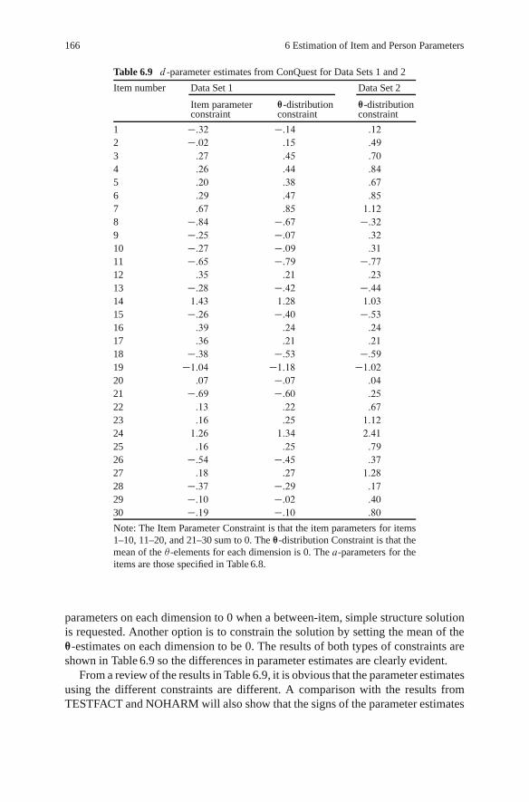
166 6 Estimation of Item and Person Parameters
Table 6.9 d -parameter estimates from ConQuest for Data Sets 1 and 2
Item number Data Set 1 Data Set 2
Item parameter ™-distribution ™-distributionconstraint constraint constraint
1 �:32 �:14 :12
2 �:02 :15 :49
3 :27 :45 :70
4 :26 :44 :84
5 :20 :38 :67
6 :29 :47 :85
7 :67 :85 1:12
8 �:84 �:67 �:329 �:25 �:07 :32
10 �:27 �:09 :31
11 �:65 �:79 �:7712 :35 :21 :23
13 �:28 �:42 �:4414 1:43 1:28 1:03
15 �:26 �:40 �:5316 :39 :24 :24
17 :36 :21 :21
18 �:38 �:53 �:5919 �1:04 �1:18 �1:0220 :07 �:07 :04
21 �:69 �:60 :25
22 :13 :22 :67
23 :16 :25 1:12
24 1:26 1:34 2:41
25 :16 :25 :79
26 �:54 �:45 :37
27 :18 :27 1:28
28 �:37 �:29 :17
29 �:10 �:02 :40
30 �:19 �:10 :80
Note: The Item Parameter Constraint is that the item parameters for items1–10, 11–20, and 21–30 sum to 0. The ™-distribution Constraint is that themean of the � -elements for each dimension is 0. The a-parameters for theitems are those specified in Table 6.8.
parameters on each dimension to 0 when a between-item, simple structure solutionis requested. Another option is to constrain the solution by setting the mean of the™-estimates on each dimension to be 0. The results of both types of constraints areshown in Table 6.9 so the differences in parameter estimates are clearly evident.
From a review of the results in Table 6.9, it is obvious that the parameter estimatesusing the different constraints are different. A comparison with the results fromTESTFACT and NOHARM will also show that the signs of the parameter estimates

6.2 Computer Programs for Estimating MIRT Parameters 167
are opposite those of the estimates from the other programs. The reason for thisdifference in sign is not clear from the expressions for the model in (4.14) and (4.15).To be consistent with the results, the exponent of the model used in the estimationprogram should be a™0�d instead of the form used by the other estimation programs– a™0 C d . There seems to be an inconsistency between the published descriptionof the estimation procedure and the model that is implemented in the program. Thecorrelation between the estimates of the d -parameter used with those from the otherprograms is .99 when the �-means are constrained to 0 and Data Set 1 is used, butthe slope of the regression line predicting the other parameter estimates from theConQuest estimates is �:69 and �:62 for TESTFACT and NOHARM, respectively.The reason the slope is not closer to 1.0 is that ConQuest uses the logistic form ofthe model while the other programs use the normal ogive form of the model. Theslope predicting the generating d -parameters that are for the logistic model is 1.2showing that the estimates are slightly regressed toward the mean compared to thetrue parameters.
The results from the analysis of Data Set 2 are similar to those from Data Set 1.The d -parameter estimates from ConQuest were correlated .99 with those from NO-HARM and TESTFACT, but the slope of the regression lines are �:66 and �:61respectively, showing the difference between the scales for the normal ogive andlogistic models. The slope would be �1=1:7 D �:58 if the shift of scale were duesolely to the differences between the normal ogive and logistic forms of the mod-els. The remaining differences are probably because of differences in the ways thatconstraints are implemented in the programs and estimation error.
ConQuest also provides maximum likelihood estimates of the ™-vectors. Theestimates are different depending on the constraints used to deal with the indetermi-nacy in the solution. For the constraint that the mean �-elements for each dimensionis 0 for Data Set 1, the mean of the estimates is very close to 0, but the standard devi-ations of the estimates are 1.31, 1.37, 1.32 for three dimensions, respectively. Thesestandard deviations are the result of fixing the a-parameters for each dimension at 1with perfect simple structure.
Table 6.10 provides summary statistics for the ™-estimates for each of the dimen-sions from the analysis of Data Sets 1 and 2. The table presents both the estimatesof population parameters for the ™-distributions given in the ConQuest output, andthe values computed from the maximum-likelihood estimates of the �s. Table 6.11presents the correlations among the ™-estimates for each data set and the correlationswith the �-values used to generate the simulated data.
From a comparison of the summary statistics from the estimated �s and thosethat are estimates of the population parameters in the model, it is clear that these arenot the same. The ConQuest manual emphasizes that point. The population corre-lation estimates are estimates of the correlations corrected for attenuation while thecalculated correlations are affected by the estimation error in the �s. The estimatesof the standard deviations are similarly affected. The important point is that the val-ues reported in the output from the program should not be interpreted as being thesame as values computed from the maximum-likelihood estimates.

168 6 Estimation of Item and Person Parameters
Table 6.10 Summary statistics for ™-distribution estimates for Data Sets 1 and 2
Data Set 1 Data Set 2
�1 �2 �3 �1 �2 �3
Mean 0 .�:02/ 0 .:02/ 0 .�:01/ 0 .�:05/ 0 .:02/ 0 .�:07/SD .90 .1:31/ .98 .1:37/ .92 .1:32/ 1.21 .1:53/ 1.33 .1:67/ .85 .1:25/Reliability .60 .62 .60 .62 .68 .85�1 1 1�2 .32 .:20/ 1 .90 .:64/ 1�3 .21 .:14/ .23 .:14/ 1 .53 .:34/ .53 .:33/ 1
Note: The values in parentheses are computed from the estimated � -values. The other values arethe estimated population parameters from the ConQuest output. The bottom three rows give thecorrelations for �s within the analysis of a data set.
Table 6.11 Correlations of estimated and generating �s forData Sets 1 and 2
Generating Data Set 1 Estimates Data Set 2 Estimatesvalues
�1 �2 �3 �1 �2 �3
�1 .75 .03 .19 .82 .71 .41�2 .00 .17 .76 .25 .26 .73�3 .23 .79 .03 .73 .86 .31
Note: Correlations are within the same data set. The generatingvalues for Data Sets 1 and 2 are not the same.
The correlations in Table 6.10 do not recover the correlations between the gen-erating �s very well. The �s used to generate Data Set 1 had intercorrelations thatwere very close to 0. The �s used to generate Data Set 2 had correlations of about.3, .8, and .2. The ConQuest correlations for neither data set approximates the gen-erating correlations. Further information is provided in Table 6.10. The relationshipbetween the generating �s and estimated �s are clearly identified for Data Set 1,but the pattern in Data Set 2 is not as evident. This result is partially because of thespecification of all a-parameters as 1 in the analysis and partially because of the cor-relations between the generating �s in Data Set 2. A comparison of Tables 6.5 and6.11 indicates that neither TESTFACT nor ConQuest provides accurate estimatesof the correlations used to generate the data. This topic will be addressed in moredetail in Chap. 7 when issues of the indeterminacy of the ™-space are discussed.
6.2.4 BMIRT
Another approach to estimating the parameters of the MIRT models has been im-plemented in a computer program called BMIRT2 (Bayesian Multivariate Item
2 BMIRT is proprietary and trade secret software developed by CTB/McGraw-Hill LLC, a sub-sidiary of the McGraw-Hill Companies, Inc. Used with permission.

6.2 Computer Programs for Estimating MIRT Parameters 169
Response Theory) (Yao 2003). This program implements Markov chain MonteCarlo (MCMC) methods using the Metropolis–Hastings sampling algorithm toestimate the item, examinee, and population distribution parameters for a set ofMIRT models for both dichotomously and polytomously scored test items.
MCMC methods are a way of generating samples from the posterior distributionof the item and person parameters given the observed item response matrix. Thegeneration is done through computer simulation. That is, observations are sampledfrom probability distributions with known properties. This is the Monte Carlo partof the process. Monte Carlo methods are quite common for generating simulateddata to test the functioning of estimation programs. The data used for the examplesin this chapter where generated using Monte Carlo simulation methods. The keyto estimation using MCMC methods is generating samples from complex distribu-tions using samples generated from known, convenient distributions. This is knownas acceptance–rejection sampling (Chib and Greenberg 1995) or simply rejectionsampling (Gamerman and Lopes 2006).
The Markov Chain part of the process is based on a statistical procedure formodeling the probability of transition from one state in a domain to another statein the domain. Suppose that there are n states – S1; S2; : : : ; Sn. These states areassumed to include all possible states in the domain. For example, the states couldrepresent the 48 states in the continental USA. If a person were limited to travelwithin the 48 continental USA, then those states would be the full set of possiblelocations for the person. At any given point in time, k, the person is located in oneof the states, Skj , and they have a probability of moving to another state or stayingin the same one at time k C 1. If the probability of moving to a state at time k C 1
is only dependent on the state at time k, then the string of locations over time islabeled a Markov chain. The probability of moving from state to state in a Markovchain can be represented by a transition matrix,
p D
2
6664
p .1; 1/ p .1; 2/ � � � p .1; n/p .2; 1/ p .2; 2/ � � � p .2; n/:::
:::: : :
:::
p .n; 1/ p .n; 2/ � � � p .n; n/
3
7775; (6.21)
where p .i; j / gives the probability of moving from Si at time k to state Sj attime k C 1. Because the person cannot move out of the domain, the values in therows must sum to 1. The probability of being in state Sj after n units of time isgiven by pn. If the rows of pn converge to the same vectors as n becomes large, theMarkov chain is said to be stationary. That is, no matter what the starting state is,the probability of being in state Sj is the same if enough steps are taken through theMarkov chain.
Stationary Markov chains provide a way of simulating the data from the sta-tionary probability distribution. If the locations in the states are recorded after eachstep of the Markov chain, then those locations provide a sample from the stationary

170 6 Estimation of Item and Person Parameters
distribution. Those observations can be analyzed to determine characteristics of thestationary distribution. A simple example should help clarify these points.
Suppose that the transition matrix for a Markov chain is given by
2
4:5 :4 :1
:1 :7 :2
:2 :3 :5
3
5 : (6.22)
This transition matrix indicates that, for example, if a person starts in S2 at timek D 0, then they would have a probability of remaining in S2 of .7 at time k D 1,and small probabilities of .1 and .2 of moving to S1 and S3, respectively. Note thateach row of the transition matrix has probabilities that sum to 1.
This transition matrix defines a stationary Markov chain. After 11 steps throughthe chain, the probability of being in each state for each starting state is
p11 D2
4:2093 :5349 :2558
:2093 :5349 :2558
:2093 :5349 :2558
3
5 : (6.23)
Thus, no matter which state is the starting state, the probability distribution forthe location in a state after 11 time periods is the same and it remains at those valuesfor additional time periods as well.
The states at each time period for this Markov chain can be simulated by selectingan initial starting state and then determining the next state by comparing a uniformrandom number to the cumulative probabilities of being in the successive states.That is, using the original transition matrix, if the starting state is S1 and the uniformrandom number is between 0 and .5, the state at time kD 1 remainsS1. If the randomnumber is greater than .5, but less than :5C :4 D :9, then the state changes to S2. Ifthe uniform random number is greater than .9, then the state changes to S3. The stateat each time period is recorded as an observation from the stationary distribution.
For the transition matrix in (6.22), a string of the first ten states for a Markovchain beginning in S1 is S1S2S3S1S3S3S1S1S2S3. From this starting state, the pro-portion of times in S1 is .4, in S2 is .2, and S3 is .4. This is not a very good matchto the stationary distribution given in (6.23) because of the dominance of the start-ing state and the short nature of the chain. However, if the chain continues on fora 1,000 time periods, the proportions are now .236, .550, and .214 – a better matchto stationary distribution over states. After 10,000 time periods, the proportions oftimes in each state are .2108, .5282, and .2610. After 100,000 time periods, the dis-tribution over states is .2094, .5353, and .2554. The proportion of times in each stateis converging to the stationary distribution, but convergence is not particularly fast.
The use of Markov chain Monte Carlo (MCMC) for MIRT estimation uses aprocess that is conceptually the same as this example. The goal is to simulate obser-vations from a stationary distribution. For estimation purposes, the Markov chain isdefined so that the stationary distribution is the posterior distribution of the modelparameters given the observed item score matrix.

6.2 Computer Programs for Estimating MIRT Parameters 171
P .™; a;d;�;¢ j X/ / P .X j ™; a;d/ P .™ j �;¢/ P .a;d/ P .�;¢/ ; (6.24)
where
P .X j ™; a;d/ DNY
jD1
IY
iD1P�Xij j ™j ; ai ; di
(6.25)
and
P .™ j �;¢/ DNY
jD1P�™j j �;¢
: (6.26)
In these equations, the ™, a, and d parameters are those of the compensatory MIRTmodel and � and � are the parameters of the assumed multivariate distribution forthe ™-vectors. The equations are used to model the item responses forN individualsto an I -item test.
In this case, the states are vectors of the model parameters – the ™-vectors forthe examinees and the item parameter vectors for the full set of items. Unlike theexample given earlier, these are continuous variables rather than discrete states. Thismeans that there is a density function that shows the transitions between states ratherthan a discrete probability distribution. The density function is called the transitionkernel t Œ and it gives the conditional density of being in a state given the currentvalues of the parameters:
th
™k; ak;dk�;™kC1; akC1;dkC1�i D P
h™kC1; akC1;dkC1� j
™k; ak;dk
�i;
(6.27)
where the superscripts indicate time k and time k C 1.The BMIRT program uses a transition kernel that is based on an approach called
Gibbs samplers (Geman and Geman 1984). This approach specifies the transitionkernel as the product of two conditional distributions. In this case, the transitionkernel is
th
™k; ak;dk�;™kC1; akC1;dkC1
�i
D P™kC1 j X; ak;dk
�P
akC1;dkC1 j X; ™kC1� : (6.28)
Because the transition kernel is partitioned into two components, the sampling ofobservations can be done in two steps. First a ™ can be drawn from its conditionaldistribution; then the sampled value can be used to specify the conditional distribu-tion for the item parameters.
The conditional distributions for the parameters are difficult to compute, sofurther refinements are added to the process. The Metropolis–Hastings algorithm(Metropolis, Rosenbluth, Rosenbluth, Teller and Teller 1953; Hastings 1970) isused to specify a more convenient transition kernel and then uses acceptance-rejection sampling to obtain observations from the desired transition kernel. Further,

172 6 Estimation of Item and Person Parameters
parameters are dealt with in blocks based on independence assumptions to simplifythe computation. The complete description of the estimation process is beyond thescope of this chapter. Patz and Junker (1999) give a fairly complete description ofthe estimation methodology as applied to unidimensional IRT models.
If the transition kernel can be specified and used to simulate the steps in theMarkov chain, then the observations from each step can be saved as a sample fromthe stationary distribution for the Markov chain. As with the example provided ear-lier, long chains are needed before the characteristics of the sample approximate thecharacteristics of the stationary distribution. Also, the initial starting states affect theresults for some time. Therefore, the initial observations from the Markov chain arediscarded. Those observations are collected during what is called a “burn in period”for the Markov chain.
The observations collected after the burn in period can be used to estimate theparameters of the stationary distribution. For example, the mean of the ™ vectorscan be used to estimate the proficiency vectors for the examinees. These wouldbe approximations to the EAP estimators of proficiency. The standard deviation ofthe distributions can be used as estimates of the standard errors for the parameterestimates. The same procedure can be used to get estimates of the item parameters.
The BMIRT computer program for estimating the parameters of the compen-satory MIRT model uses a transition kernel designed to give the stationary distri-bution specified in (6.24). The states specified by the transition kernel are the fullset of item parameters, the vectors of person parameters, and vector for the meanperson parameters and the variance/covariance matrix for the person parameters.Although the MCMC approach implemented in BMIRT is very powerful, it still re-quires user specified constraints to address the indeterminacy of the origin, scale,and rotation for the model. BMIRT addresses these issues requiring that the userspecify a population mean vector and variance for each dimension, and identify atleast one item to anchor each scale. The anchor item approach is the same as is usedby the NOHARM program. The user is also asked to specify the number of obser-vations to discard as “burn in” before using the sampled observations to estimate theparameters. The sample size for estimating the parameters also needs to be specified.
The BMIRT program was used to estimate the parameters for the same two datasets used as examples for TESTFACT and NOHARM. For the analyses, the meanvector for ™ was specified as the 0-vector and the variances were specified as 1.0.Also, the first item of each of the ten item sets related to a dimension was usedto anchor the axes of the coordinate space to deal with the rotational indetermi-nacy for the model. The program was run with 10,000 samples discarded as burnin and 20,000 iterations used to generate the sample for estimating the parameters.The program took approximately 45 min to converge on the estimates on a note-book computer with a Pentium 1,400 MHz processor. The item parameter estimatesfrom the program are given in Table 6.12. The b-parameter estimates have the signsreversed relative to the generating parameters because the dichotomous item re-sponses were analyzed as a special case of the partial credit model with two scorecategories. That model has a “�d” in the exponent instead of the “Cd” used in thegenerating model.

6.2 Computer Programs for Estimating MIRT Parameters 173
Table 6.12 Item parameter estimates for Data Set 1 and Data Set 2
Item number Data Set 1 Data Set 2
a1 a2 a3 d a1 a2 a3 d
1 .22 .00 .00 �:12 1.19 .00 .00 :12
2 .21 .21 .46 :14 .55 .24 .22 :40
3 .24 .35 1.04 :47 1.20 .40 .30 :70
4 .25 .21 1.19 :48 .91 .28 .44 :78
5 .22 .33 .59 :36 .67 .29 .25 :57
6 .27 .39 1.22 :52 2.24 .97 .53 1:22
7 .40 .50 1.62 1:06 1.80 .73 .42 1:39
8 .22 .30 .87 �:66 1.26 .37 .35 �:349 .22 .31 1.12 �:07 1.48 .36 .29 :34
10 .23 .24 .96 �:09 1.28 .49 .27 :31
11 .30 .85 .00 �:75 1.01 .80 .00 �:7512 .22 1.15 .27 :23 1.14 1.25 .25 :25
13 .22 .76 .24 �:38 .80 .60 .22 �:3914 .27 2.14 .34 1:79 2.15 1.90 .48 1:59
15 .22 .91 .23 �:38 .88 .85 .23 �:5016 .22 .99 .22 :25 1.06 .90 .24 :25
17 .26 1.56 . 22 :27 1.42 1.37 .45 :25
18 .39 .98 .26 �:52 .91 .98 .23 �:5919 .40 1.03 .24 �1:19 .80 .72 .40 �:9520 .21 .69 .21 �:06 .64 .66 .22 :04
21 1.22 .23 .22 �:65 .34 .26 .91 :25
22 .49 .21 .24 :20 .23 .22 .50 :62
23 1.18 .34 .31 :27 .71 .44 1.09 1:27
24 2.10 .30 .24 1:87 .30 .30 1.51 2:88
25 .66 .21 .21 :23 .25 .25 .65 :75
26 1.34 .24 .23 �:50 .33 .33 1.17 :39
27 1.68 .24 .24 :34 .24 .30 1.14 1:39
28 .62 .21 .21 �:26 .21 .22 .49 :15
29 .53 .21 .23 �:01 .26 .22 .57 :37
30 1.18 .26 .23 �:11 .39 .36 .92 :83
Note: The largest a-parameter for each item is shown in bold italics.
The a-parameter estimates clearly recover the structure of the data for the simplestructure case. There are two interesting anomalies in the solution. First, even thoughItem 1 was used to anchor one of the axes, that item is not correctly estimated assensitive to differences on the same dimension as the other items in the first ten.It has a 0 a-parameter on the third coordinate axis. This poor estimation of theparameters for Item 1 did not seem to interfere with the estimation of the parametersfor the other items. To check the functioning of the program, the parameters for thisdata set were estimated a second time starting with a different random seed number.This analysis gave a .88 a-parameter for the first item and similar item parameterestimates for all of the other items. This result suggests that the BMIRT programshould be run more than once on a set of data using different starting values todetermine if the parameter estimates are stable.

174 6 Estimation of Item and Person Parameters
Table 6.13 Summary statistics for ™ distribution estimates for Data Sets 1 and 2
Data Set 1 Data Set 2
�1 �2 �3 �1 �2 �3
Mean :001 �:001 :001 �:007 �:004 �:008SD :79 :79 :75 :81 :63 :71
�1 1:00 1:00
�2 �:04 1:00 :48 1:00
�3 �:02 :02 1:00 :10 :10 1:00
Table 6.14 Correlations of estimated and generating �s for Data Sets 1 and 2
Generating values Data Set 1 Estimates Data Set 2 Estimates
�1 �2 �3 �1 �2 �3
�1 :14 �:03 :76 .84 .51 .27�2 :79 :09 �:08 .20 .23 .74�3 �:03 :81 :13 .81 .74 .14
Note: Correlations are within the same data set. The generating values for DataSets 1 and 2 are not the same.
The second anomaly is that none of the a-parameter estimates are below .2 evenwhen the generating item parameters are close to 0. This was true for both analysesof the data set of the first data set and for the second data set. This may be a result ofthe priors specified in the program. Despite these unusual results, the parameter es-timates for the first data set provide a close match to the generating parameters. Thea-parameter estimates for the second data set tend to be over-estimates and the pro-gram tends to merge the two dimensions that have generating �s correlated .8. Thisresult is similar to that found for TESTFACT (Table 6.3) and NOHARM (Table 6.6).All of these programs have difficulty separating the dimensions when the �s on thosedimensions are highly correlated.
Table 6.13 presents the descriptive statistics for the ™-estimates from the BMIRTprogram for the two data sets. The mean �s are very close to 0, but the standarddeviations are not 1.0. The standard deviations in Data Set 2 are not equal and tendto reflect the differences in standard deviations used to generate the data. The cor-relations between �s for Data Set 1 match the uncorrelated �s used to generate thedata. The correlations for Data Set 2 do not recover the correlational structure usedto generate the data. To further investigate the relationships between the generatingand estimated �s, these variables were correlated with each other. The results arepresented in Table 6.14.
The correlations of the ™-estimates with the generating �s show that BMIRTrecovered the underlying structure of the data well for Data Set 1, the data setgenerated with uncorrelated �s. The correlation between the estimated �s and thegenerating �s is as high as can be expected from a test with ten items sensitive todifferences on each dimension. The correlational structure underlying Data Set 2was not well recovered by BMIRT. Dimensions 1 and 2 for the estimated �s were

6.3 Comparison of Estimation Programs 175
both correlated with Dimension 3 from the generating �s. This is because of thehigh correlation between Dimensions 1 and 3 for the �s used to generate the data.BMIRT gave what is essentially a two-dimensional solution for the data set withthe two highly correlated ™-dimensions used to generate the data being estimatedas a single common dimension. It is possible that the Data Set 2 solution can berotated and translated to better match the parameters used to generate the data. Thispossibility will be address in Chap. 7.
6.3 Comparison of Estimation Programs
The application of MIRT procedures is dependent on the quality of parameter es-timates that are obtained from the estimation programs. The programs that areavailable vary in the estimation procedures used and the way that they address theindeterminacy issues of the MIRT models. The programs also differ in the types ofmodels that they support and whether they estimate the person parameter vectors.Further, the programs differ in the number of dimensions that they can estimate andthe computer resources needed to implement the estimation procedure. Some pro-grams are very fast, but have limited capabilities. Others take substantial amounts ofcomputer time to converge on estimates, but can handle a wide variety of applica-tions. While different statistical estimation methods can be compared on theoreticalcharacteristics such as whether the estimators are unbiased, efficient, etc., in practicethe estimation methods cannot be evaluated independently of the computer softwareused to implement them. A theoretically optimal estimation method may not havesuch properties in practice because approximations were used when developing theestimation software. Because of the interconnectedness of the statistical estimationmethodology and the software used to implement it, methods are often evaluated us-ing parameter recovery studies based on computer simulations. The results of someparameter recovery studies are summarized here. This summary should be used withsome caution because some programs are updated regularly and the results may nolonger apply. The information provided here was collected in July 2007.
Because it is impossible to know how soon the information about programs willbecome dated, the information presented here will only cover general trends ratherthan the details about specific estimation programs. It is also recommended thatnew estimation software be investigated as it becomes available. New estimationmethods may supersede those presented here.
The majority of comparative studies that were available at the time this chap-ter was written consider the NOHARM and TESTFACT software. These pro-grams have been available much longer than the others. The general finding ofthe comparative studies (Beguin and Glas 2001, Gosz and Walker 2002, Maydeu-Olivares 2001, Miller 1991, Stone and Yeh 2006) was that neither NOHARM norTESTFACT is clearly superior to the other when considering the recovery of itemparameters. Each program performs better than the other for specific situations, but

176 6 Estimation of Item and Person Parameters
the results are for a particular number of examinees administered a test of a specifiednumber of items with a specific item structure and pattern of correlations between�s used to generate data. It is difficult to generalize these results to the analysis ofnew data sets.
There are practical differences in the two software packages. NOHARM doesnot provide estimates of the ™-vectors – a clear limitation. TESTFACT does provideestimates of the ™-vectors. NOHARM requires less computer time than TESTFACT,but with the speed of current computers, the differences in computational time arenot of practical importance. TESTFACT is limited in the number of dimensions thatcan be estimated because of the way the full information aspect of the program usescomputer storage. NOHARM does not have that limitation and special versions ofthe program have been used to estimate as many as 50 dimensions.
In contrast to the comparative studies for NOHARM and TESTFACT, only onestudy was found comparing ConQuest to another program and that was to a newprocedure with limited availability (Moulton 2004). There have also been a fewstudies that compare ConQuest and other programs for estimating the parameters ofthe unidimensional Rasch model, but those are not the focus of this chapter.
Research articles have begun to appear comparing MCMC procedures with NO-HARM or TESTFACT (Bolt and Lall 2003). The results of these studies haveindicated that the MCMC procedures tend to have larger standard errors for theparameter estimates than NOHARM. It is difficult to judge the generalizabilityof these studies because the results depend on the particular implementation of aMCMC procedure. The Bolt and Lall (2003) study used their own implementa-tion of MCMC using WinBUGS software (Spiegelhalter, Thomas, and Best 2000)and the results may not generalize to the BMIRT software described earlier in thischapter.
At the time this chapter was written, NOHARM or TESTFACT still seem to bethe programs of choice if the test data consists of dichotomous item responses. NO-HARM is a free program that gives quick estimates of item parameters. TESTFACTis a more flexible program that provides estimates of ™-vectors as well as item pa-rameters. Because TESTFACT is not a free, it has the advantage of having updatedversions and more complete documentation. This chapter did not review all softwarethat is available for MIRT calibration. Other programs may be available and someof them may function very well.
6.4 Exercises
1. The example on p. 141 of this chapter considers the likelihood function for itemscore vector Œ1 0. Using the item parameters for the same test items given in thatexample, consider the likelihood function for the item score vector Œ0 1. Where inthe region of the ™-space defined by the range from �4 to 4 on each coordinate axeswill the likelihood be the greatest for the item score vector Œ0 1?

6.4 Exercises 177
2. A test item is modeled with two coordinate axes. When the normal ogive ver-sion of the compensatory model is used the item parameters are a1 D :5; a2 D :5;
and d D � 1:7. Assuming that the two discrimination parameters are equal fora logistic version of the model, what logistic model item parameters will givethe item characteristic surface that gives the closest match to the normal ogiveversion?
3. For each program described in this chapter, indicate whether it uses maximumlikelihood, marginal maximum likelihood, generalized least squares, Bayes modalestimation, Bayes expected a posteriori estimation, or Markov chain Monte Carloestimation.
4. A gambler suspects that a coin has been tampered with so that it will land “heads”75% of the time when flipped. Suppose the coin was flipped one time and landed“heads.” The belief before the coin flip was that there were even chances that thecoin was tampered with or fair. What is the posterior probability that the coin is a“fair” coin (.5 probability of a head) or the tampered with coin?
5. Which of the constraint options in ConQuest is consistent with an assumptionthat sets of items that measure different constructs are of equal difficulty on average?Summarize the rationale for your answer.
6. Which two of the MIRT model calibration programs described in the chapter usethe most similar statistical estimation procedure? Briefly summarize that procedureand indicate how the two programs differ in the implementation of the methodology.
7. Use the item parameters used to create Fig. 6.4 to determine the maximum like-lihood estimator for the item score string 011. How does this estimate differ fromthe maximum likelihood estimate for the item score string 100?
8. What computer program would you select if you wanted to estimate the itemparameters for a test specifying fixed guessing parameters and aligning 12 contentdimensions with coordinate axes? Summarize the features of the program that leadto its selection.
9. How does NOHARM remove the rotational indeterminacy in the estimates ofitem parameters? Give a practical example of how you would implement this systemof constraints if a test contains 40 items with 10 items written to be sensitive todifferences along each of four different constructs.
10. The a-parameters were estimated for the items on a simulated test using theTESTFACT program. The item score data for the test were generated using (4.5)and a multivariate normal distribution with an identity matrix for the correlationsamong �s. What relationship is expected between the estimated a-parameters andthose used to generate the data?

178 6 Estimation of Item and Person Parameters
11. Suppose that a third data set was generated using the item parameters inTable 6.1. The third data set has a zero mean vector for the �s and standarddeviations of 1.0, and all the intercorrelations are .8. How would the statisticalanalysis results for this data set compare to those given in Table 6.2? Explain thereasoning behind your prediction.
12. If both item and person parameters are estimated, how many parameters needto be estimated for the model presented in (4.5) for a four-dimensional solution fora test of 50 items administered to 5,000 persons?

Chapter 7Analyzing the Structure of Test Data
One of the common uses of MIRT is the analysis of the structure of the item re-sponse data that results from the administration of a set of test items to a sample ofexaminees. This type of analysis can be done in either an exploratory or confirma-tory way. The exploratory analysis of item response data is used when either thereis no clear hypothesis for the structure of the item response data, or when an uncon-strained solution is seen as a strong test of the hypothesized structure. Confirmatoryanalyses require a clear hypothesis for the structure of the item response data. Thatis, there must be hypotheses about the number of coordinate dimensions needed tomodel the data and the relationship of the item characteristic surface to the coor-dinate axes. The types of confirmatory analyses that are typically done specify therelationship of the direction best measured by a test item (the direction of maximumdiscrimination) with the coordinate axes. It is also possible to have hypotheses aboutthe difficulty of test items, but such hypotheses are seldom checked with the MIRTmodels. The difficulty parameters are typically left as parameters to be estimatedwithout constraints.
In many cases, what is labeled as an exploratory analysis also has a confirmatoryanalysis component because the number of coordinate dimensions is selected priorto estimating the item and person-parameters. The resulting measures of fit of themodel to the data are a test of a hypothesis about the number of dimensions. Becausethe number of coordinate dimensions is a critical component of both exploratoryand confirmatory analyses, this issue will be addressed first. After consideration ofthe number-of-dimensions problem, procedures are described for determining thestructure of item response data using exploratory and confirmatory procedures.
7.1 Determining the Number of Dimensions for an Analysis
Approaches for determining the number of dimensions for a multidimensionalanalysis of test data has a long history in the literature on factor analysis. For exam-ple, Holzinger and Harman (1941, pp. 64–68) determined the number of variablesneeded to support the estimation of the factor loadings for m independent factors.
M.D. Reckase, Multidimensional Item Response Theory, Statistics for Socialand Behavioral Sciences, DOI 10.1007/978-0-387-89976-3 7,c� Springer Science+Business Media, LLC 2009
179

180 7 Analyzing the Structure of Test Data
The following expression gives the number of variables, n, needed to support theestimation ofm independent factors.
n � .2mC 1/C p8mC 1
2: (7.1)
This expression was derived assuming no error in the estimation of correlations.Thurstone (1947) suggested that the number of variables needed for a convincinganalysis with m factors should be “two or three times greater” than this number.For a solution with three coordinate axes, a minimum of six variables is needed, butThurstone recommends 12–18 to yield a convincing result.
Thurstone (1947) also specified a principal of factor analysis that has carriedforward to this day and is also used by many who perform MIRT analyses. “Thescientific problem is to account for as much as possible of the relations betweentests by the smallest possible number of common factors” (p. 82). Although manysubscribe to this principal, the position taken in a later section of this chapter is thatthe number of coordinate axes should be more than the minimum needed to accountfor the relationships in the data so that solutions are not misleading in certain ways.A thorough discussion of this topic is given in Sect. 7.1.1.
The seminal work on factor analysis done by Thurstone also made the importantpoint that the factor analysis solutions are dependent both on the set of variablesin the analysis and the selection of persons that are measured on these variables.Even for the case of simple structure (each variable loading on a single coordinateaxis), the correlations between the factors are dependent on the characteristics ofthe persons in the sample (Thurstone 1947, p. 440). This is an extremely importantpoint that will be elaborated upon in the next pages of this chapter.
The concept of simple structure will be referenced a number of times in thischapter so it is useful to give it a formal definition here. Thurstone (1947) gave thisconcept a very specific meaning.
“The combination of a test configuration and the co-ordinate axes is called a structure. Theco-ordinate axes determine the co-ordinate planes. If each test vector is on one or more ofthe co-ordinate planes, then the combination of the configuration and the co-ordinate axesis called simple structure. The corresponding factor pattern will then have one or more zeroentries in each row.” p. 181 (Italics in the original)
This definition of simple structure is more general than current usage because itallows test items to have nonzero a-parameters on more than one dimension. Onlyone zero a-parameter is needed for Thurstone to label the solution as simple struc-ture. Current usage is more restrictive in that it tends to allow only one nonzeroa-parameter for each item. Approximate simple structure is used when test itemshave one large a-parameter and the others are near zero. When this is the case, theitem arrows point along the coordinate axes. In this chapter, the more restrictivedefinition of simple structure is used.
The early work on factor analysis was more concerned with specifying theamount of data for an analysis with a specified number of dimensions than withthe problem of determining the number of dimensions needed to model the data.

7.1 Determining the Number of Dimensions for an Analysis 181
This probably reflects the problems of obtaining factor analytic solutions at a timewhen work was done on large main-frame computers or mechanical calculators.As computing power increased, the issue of number of dimensions has becomemore important, but the solution to the number of dimensions problem seems tobe unsolved. Reise et al. (2000) summarize the research on selecting number of di-mensions and conclude that it is better to overestimate the number of dimensionsthan underestimate them and that scree plots, parallel analysis, and analysis of theresidual correlation matrix are as good as more elaborate procedures for determin-ing the dimensionality needed to model a matrix of test data. Econometricians havestarted to notice this problem and have addressed it using fit indexes based on theAIC and BIC measures (Bai and Ng 2002). It is interesting that Bai and Ng (2002)see the problem as determining the “true number of factors.” The position takenhere is that a true number of dimensions does not exist, but that a sufficient numberof dimensions is needed to accurately represent the major relationships in the itemresponse data. If the fine details of the relationships in the data are of interest, moredimensions are needed to accurately show those details. Using too few dimensionsresults in projecting the complexities of the relationships into a smaller space thanis necessary to show the relationships. The result is that people and items can ap-pear similar when they differ on important features. The next section provides someempirical examples to set the stage for later development.
7.1.1 Over and Under-Specification of Dimensions
Item response data from real tests is generated through a very complex interactionbetween people and the test tasks. The people vary in a large number of ways andthe test tasks require numerous skills including decoding of language and otherspecialized symbols such as mathematical or chemical notation. As a result, all datamatrices from the administration of real tests are likely to require a large number ofdimensions to accurately represent the relationships in the data. At the most extreme,each test item can be considered to measure a somewhat different construct andan n-item test can be thought of as requiring n-dimensions to represent all of therelationships.
The extreme position is probably correct in a purely mathematical sense becauseall N � n data matrices, where N is the number of examinees, n is the numberof test items, and N > n, have a rank that is very likely n. However, there is stillvalue in determining if a smaller number of dimensions can be used to representmajor relationships in the data. This means the ignoring dimensions needed to modelminor relationships that are incidental to the main purpose of the test is not seen asa deficiency. For example, not being able to determine that some portion of theperformance on a test item is related to the location of a test item on the page ofa test booklet is acceptable when the purpose of the test is to measure skills inmathematics. Of course, that is only true if the effect of location on the page is verysmall relative to the influence of mathematical skills.

182 7 Analyzing the Structure of Test Data
When the number of dimensions used to model an item response matrix is pur-posely minimized to only identify the major features of the data matrix, there is adanger that the meaning of constructs will be confused rather than clarified. Thiscan happen because the locations of persons and items are projected from a high di-mensional space to a lower dimensional space. This can make person locations seemclose when they are not or test items seem to be sensitive along the same dimensionswhen they are not. This can happen because person locations or item vectors may beprojected on top of each other when they really have large distances between themin the higher dimensional space. This is a common phenomenon when we look atstars in the night sky. Two stars may appear to be close to each other when they arereally far apart. The illusion of proximity results from the star locations being on thesame line of sight from the location of the observer. Their three-dimensional loca-tions are being projected onto a two-dimensional plane. The stars may be far aparton the third dimension, even though their two-dimensional projections are close toeach other.
One way to avoid the problem of projecting persons or test items in a way thatmakes them appear similar when they are not is to use more dimensions for anal-ysis than is thought to be necessary to accurately represent the data. The relativelocations of points stay the same when they are analyzed in more than enoughdimensions. However, there is a price to be paid for using more than enough di-mensions. More person and item parameters must be estimated and that may resultin increased estimation error.
An underlying premise of this chapter is that number of dimensions needed to ac-curately model the relationships in the item response matrix is dependent on two as-pects of the data collection process – the number of dimensions on which the peopletaking the test differ and the number of dimensions on which test items are sensitiveto differences. In the most extreme cases, it is possible to imagine a group of indi-viduals who have been carefully selected to be identical on all dimensions exceptone. Because this set of individuals only varies on one dimension, the item responsematrix that results from administering any test to them can represent differences ononly one dimension, no matter what the test items are designed to measure. Simi-larly, if the set of test items used in a test are only sensitive to differences along oneof the dimensions of variability of the examinee population, the resulting data willbe well fit by a model with a single � , even though the examinees differ in many dif-ferent ways. Thus, the position taken here is that the number of dimensions neededto accurately model a matrix of item response data is the smaller of the dimensionsor variation for the people and the dimensions of sensitivity for the test items.
The literature on assessing the number of dimensions needed to accurately modelitem response data is somewhat imprecise in the way that the term “dimensionality”is used. For example, Mroch and Bolt (2006) take the following position: “Due to themultidimensional nature of many psychological and educational tests, proceduresthat identify test dimensional structure can be helpful for test practitioners” (p. 67).This statement implies that dimensionality is solely a feature of the test. No mentionis made of the dimensions of variability of the examinees. The authors probablymean to focus on the dimensions of sensitivity of the test items, but this is not

7.1 Determining the Number of Dimensions for an Analysis 183
clearly stated. It is also important when evaluating the sensitivity of test items thatthe examinees in the sample vary on dimensions that are the focus of the items. Thenumber of dimensions needed to model the item response matrix may be differentdepending on the amount of variability on the dimensions in different samples ofexaminees.
The next part of this section demonstrates the main points of the introductorycomments using the analysis of simulated item response data. Two cases are con-sidered. The first case is that test items are sensitive to examinee differences on anumber of dimensions (three for the example), and the amount of variation on thedimensions for the examinees is manipulated when generating the simulated itemresponse data. The simulated examinees are either well spread on all the three di-mensions or are distributed along a single composite of the dimensions, falling alonga line in the three-dimensional space.
The second case is that the items are sensitive to a single composite of dimen-sions, but the examinee sample varies on all three dimensions. This case does notrequire that the test items measure a single construct, but that they all measure thesame weighted combination of a set of constructs. It is shown that the data generatedin this case is indistinguishable from data that are generated using a model with asingle � .
Case 1: Items Sensitive to Variation on Three Dimensions
The parameters for the test items used for this example are the same as those usedfor the demonstration of estimation procedures in Chap. 6. These item parametersare listed in Table 6.1. This test is composed of three sets of ten test items, each withtheir direction of greatest discrimination along one of the three coordinate axes. Theitem arrows for these items are shown in Fig. 7.1.
The item parameters were used with ™-vectors randomly sampled from twodistributions to generate item response data. In both cases, 5,000 ™-vectors weresampled from the distributions. The first distribution of ™s was the three-dimensionalmultivariate normal distribution with mean vector 0 and the identity matrix for thevariance/covariance matrix. For convenience, the data set generated with the itemsand these ™-vectors is labeled 3d. The second distribution also has a mean vector
of 0, but the variance/covariance matrix is
2
4:1670 :2362 :2892
:2362 :3340 :4091
:2892 :4091 :5010
3
5. This matrix
yields a correlation matrix with 1s in all locations indicating that the matrix is ofrank 1. All the ™-vectors have three values, but the points they define fall alonga line in the ™-space. The data set generated using the item parameters and these™-vectors is labeled 3d1 because the items are sensitive to differences along threedimensions, but the people vary along a single composite score. In all cases, the datawere generated assuming the multidimensional generalization of the two-parameterlogistic model.

184 7 Analyzing the Structure of Test Data
–1–0.5
00.5
1
–1–0.500.511.5–1.5
–1
–0.5
0
0.5
1
1.5
θ2
θ 3
θ1
Fig. 7.1 Item arrows in three-dimensional ™-space
The two data sets were analyzed with TESTFACT specifying one, two, three,or four dimensions. These data were also analyzed using the unidimensional IRTestimation program, BILOG MG (Zimowski et al. 2003), to determine how the uni-dimensional estimates of � corresponded to the multidimensional estimates. The�-estimates from the BILOG MG analysis of the 3d and 3d1 data sets correlated.9998 and .9996, respectively, with the estimates from TESTFACT when one di-mension is extracted. It is clear that BILOG MG is essentially a program to estimatethe largest single factor from a set of data.
According to Wang (1985), when a unidimensional model is fit to multidi-mensional data, the result is an estimate of �s along the reference compositefor the test (see Sect. 5.3 of Chap. 5). The direction of the reference com-posite can be determined by treating the eigenvector corresponding to thelargest eigenvalue of the a0a matrix as a vector of a-parameters. For the setof items in Table 6.1, the eigenvector corresponding to the reference compositeis Œ:44 :55 :71. The procedures described in Sect. 8.1.2 of Chap. 8 can be usedto rotate the first axes of the ™-space to align with the reference composite.After that is done, the values of �1 in the vectors of person parameters are esti-mates of location along the reference composite. The rotation to align with thereference composite was computed resulting in the following rotation matrix:2
4:44 �:78 �:44:55 :62 �:55:71 0 :71
3
5. The ™-coordinates were transformed using this rotation
matrix and the results were correlated with the estimates of � obtained from theone-dimensional solutions from TESTFACT and BILOG MG. The resulting corre-lations along with the means and standard deviations for the �-values are presented

7.1 Determining the Number of Dimensions for an Analysis 185
Table 7.1 Correlations of unidimensional � -estimates, the reference composite, and the generat-ing �s for the 3d data set
BILOG TESTFACT 1d 3d reference �1 �2 �3
composite
BILOG 1:0000
TESTFACT 1d :9998 1:0000
3d referencecomposite
:8637 :8644 1:0000
�1 :4564 :4524 :4423 1:0000
�2 :5071 :5060 :5611 :0172 1:0000
�3 :5518 :5561 :7119 �:0004 :0119 1:0000
Mean :0000 :0020 :0422 :0157 :0372 :0207
Standarddeviation
:8793 :8561 1:0222 1:0055 1:0060 1:0211
in Table 7.1. Note that the standard deviations of the BILOG and TESTFACTestimates have not been scaled to have a standard deviation of 1.0. These programshave a default scaling that has the sum of the error variance and true score varianceequal to 1.0. There is also an option in the programs to scale the estimates to have astandard deviation of 1.0.
The results in the correlation matrix show that the estimates from BILOG MGand TESTFACT have almost identical correlations with both the reference compos-ite and the �s used to generate the data. Also, the correlations with the referencecomposite are as high as is allowed by the error in the estimates from the programs.The estimated reliability of the BILOG MG estimate is .736. The correlation be-tween the BILOG MG estimates and the reference composite is approximately 1.0when corrected for attenuation.
BILOG MG provides a 2 measure of fit for the unidimensional IRT model, inthis case the two-parameter logistic model, to the data from each item. Of the 30 testitems on this simulated test, the model showed significant deviations from the datafor 16 items at the .05 level of significance. This is surprisingly good fit for the dataconsidering the sample size is 5,000, the data were generated using uncorrelated�s, and sets of items were sensitive to differences along each of the coordinateaxes. TESTFACT provides a 2 test of fit for the full model. In this case, the onefactor solution had a 2 value of 108686.23 with 4,939 degrees of freedom. Thisindicates that the one-dimensional model did not do a very good job of representingthe relationships in the data file. These fit measures will be discussed in more detaillater in this chapter.
The same matrix of item response data was also analyzed using TESTFACTspecifying a two-dimensional solution. The item arrows from that two-dimensionalsolution are presented in Fig. 7.2. The items that are sensitive to differences alongthe �1 and �2-axes are clearly evident in the figure. However, the items that aresensitive to differences along the third coordinate axis are projected into the two-dimensional space as item vectors that fall roughly along a 45ı line between theother two axes. This gives the appearance that the third set of items is sensitive
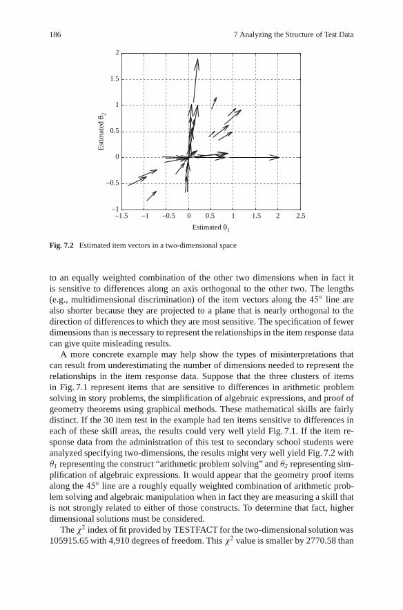
186 7 Analyzing the Structure of Test Data
–1.5 –1 –0.5 0 0.5 1 1.5 2 2.5–1
–0.5
0
0.5
1
1.5
2
Estimated θ1
Estim
ated
θ2
Fig. 7.2 Estimated item vectors in a two-dimensional space
to an equally weighted combination of the other two dimensions when in fact itis sensitive to differences along an axis orthogonal to the other two. The lengths(e.g., multidimensional discrimination) of the item vectors along the 45ı line arealso shorter because they are projected to a plane that is nearly orthogonal to thedirection of differences to which they are most sensitive. The specification of fewerdimensions than is necessary to represent the relationships in the item response datacan give quite misleading results.
A more concrete example may help show the types of misinterpretations thatcan result from underestimating the number of dimensions needed to represent therelationships in the item response data. Suppose that the three clusters of itemsin Fig. 7.1 represent items that are sensitive to differences in arithmetic problemsolving in story problems, the simplification of algebraic expressions, and proof ofgeometry theorems using graphical methods. These mathematical skills are fairlydistinct. If the 30 item test in the example had ten items sensitive to differences ineach of these skill areas, the results could very well yield Fig. 7.1. If the item re-sponse data from the administration of this test to secondary school students wereanalyzed specifying two-dimensions, the results might very well yield Fig. 7.2 with�1 representing the construct “arithmetic problem solving” and �2 representing sim-plification of algebraic expressions. It would appear that the geometry proof itemsalong the 45ı line are a roughly equally weighted combination of arithmetic prob-lem solving and algebraic manipulation when in fact they are measuring a skill thatis not strongly related to either of those constructs. To determine that fact, higherdimensional solutions must be considered.
The 2 index of fit provided by TESTFACT for the two-dimensional solution was105915.65 with 4,910 degrees of freedom. This 2 value is smaller by 2770.58 than

7.1 Determining the Number of Dimensions for an Analysis 187
Table 7.2 Correlations be-tween �s used to generatedata and TESTFACT two-dimensional estimates
Generating TESTFACT �s�s �1 �2
�1 .23 :36
�2 .11 :75
�3 .80 �:01
the value for the one-dimensional solution with a difference in degrees of freedomof 29. The improvement of the fit of the two-dimensional model over the one-dimensional model is dramatic, but the overall fit of the model is still not good.The overall 2 indicates that the observed data is significantly different than thatpredicted by the two-dimensional MIRT model.
The effect of using too few dimensions to represent the relationships betweenpersons and items can also be seen in the correlations between the elements of theestimated ™-vectors for the two-dimensional solution and the elements of the three-dimensional ™-vectors used to generate the item response data. These correlationsare given in Table 7.2. The estimated �s provide fairly good recovery of the �2 and�3-coordinates from the generating �s, but �1 has only a small influence on theestimated �s. The � that is projected between the other dimensions is difficult topredict. It is likely related to the variance accounted for by the sets of items relatedto each dimension.
The effect of using too many dimensions can be seen from the analysis of thisexample data set with TESTFACT specifying four dimensions. The item parameterestimates that result from that analysis are provided in Table 7.3 along with theparameters used to generate the data. The correlations between the estimated �sand the generating �s are given in Table 7.4.
Inspection of Table 7.3 shows the relationships between the estimated item pa-rameters and those used to generate the data. The sets of item parameters andestimates that are most sensitive to differences along each coordinate axis are shownin bold italics. The order of the ™-estimates from TESTFACT is not the same asthat for the generating parameters. The TESTFACT order is related to the averagea-parameter for each dimension. However, it is easy to see the sets of items thatare sensitive to differences along each construct. In fact, the correlations betweenthe corresponding sets of item parameters are uniformly in the high .90s with thecorrelation between the d -parameter estimates and the generating values close to1.00. Note that the estimated values and the generating parameters differ by theconstant D D 1:7 because of differences between the logistic model used to gen-erate the data and the normal ogive model used for estimation. Also, the values ofthe a4-parameter estimates are generally low, and there is no relationship betweenthose parameter estimates and those used to generate the data. It is clear that thesimulated test items are not distinguishing among ™-points along the unnecessary4th coordinate axis.
The same pattern is evident in the correlations between the estimated �s from thefour-dimensional solution using TESTFACT and the �s used to generate the itemresponse data. The estimated �-coordinates for dimensions 1, 2, and 3 correlatehighly with generating �-coordinates. The estimated �s for the fourth coordinate

188 7 Analyzing the Structure of Test Data
Table 7.3 Generating and TESTFACT estimated item parameters using four dimensions
Item number Generating item parameters TESTFACT estimated item parameters
a1 a2 a3 d a1 a2 a3 a4 d
1 .75 .03 .14 :18 .05 .11 .43 :02 :13
2 .46 .01 .07 �:19 .03 .05 .29 :27 �:113 .86 .01 .40 �:47 .18 .02 .53 �:11 �:294 1.01 .01 .05 �:43 �:08 .08 .54 :13 �:295 .55 .02 .15 �:44 .05 .05 .34 :05 �:276 1.35 .01 .54 �:58 .16 .07 .81 :04 �:357 1.38 .09 .47 �1:04 .16 .11 .82 :10 �:578 .85 .04 .26 :64 .04 .05 .58 :07 :40
9 1.01 .01 .20 :01 .03 .04 .63 �:07 :04
10 .92 .01 .30 :09 .12 .06 .59 :04 :05
11 .00 .24 .80 :81 .44 .16 .07 �:16 :52
12 .00 .19 1.19 �:19 .71 .03 .10 :00 �:1013 .06 .09 .71 :45 .46 .01 .08 :04 :27
14 .02 .33 2.14 �1:84 1.22 .06 .16 :09 �1:1015 .03 .05 .86 :41 .51 .03 .11 :13 :26
16 .02 .15 .93 :30 .60 .10 .06 :10 �:1617 .03 .29 1.36 :18 .82 .11 .10 �:04 �:1018 .00 .22 .90 :51 .55 .12 .06 �:05 :29
19 .00 .47 .73 1:13 .46 .21 .04 :01 :68
20 .01 .09 .64 :02 .39 .05 .11 :01 :02
21 .31 .97 .00 :62 �:01 .56 .15 �:08 :38
22 .18 .50 .00 �:20 .04 .29 .07 :09 �:1323 .41 1.11 .20 �:37 .11 .72 .25 �:20 �:2124 .15 1.73 .03 �1:76 .13 .95 .03 �:01 �:9625 .15 .67 .00 �:24 .04 .42 .01 :03 �:1626 .29 1.24 .02 :49 .10 .71 .13 :07 :31
27 .13 1.49 .00 �:34 .08 .91 .02 �:06 �:1828 .05 .48 .00 :29 .04 .33 .01 :00 :21
29 .21 .46 .01 :01 .01 .31 .12 :14 :01
30 .18 1.12 .09 :03 .09 .65 .13 �:13 :05
Note: The TESTFACT estimates differ from the generating parameters by the constant D D 1:7
because of differences between the logistic and normal ogive model
axis, however, do not correlate highly with any of the dimensions and it has a fairlysmall standard deviation as well. The magnitude of the correlations between esti-mated and generating �s, approximately .8, is consistent with the amount of errorthat results from estimating person locations with a 30-item test.
The results from these examples show that using too many dimensions gives asolution that embeds the dimensional structure needed to explain the relationshipsbetween item responses in a higher dimensional ™-space. The unneeded dimensionsare there, but they do not add to the information about the locations of personsin the space. The results also show that the dimensionality of the solution is lim-ited by the dimensions of variation of the examinee sample. Even if test items aresensitive to differences on several dimensions, unless the examinees also vary along

7.1 Determining the Number of Dimensions for an Analysis 189
Table 7.4 Correlations between generating and estimated �s for the four-dimensional solution
Generating �s Estimated �s
�1 �2 �3 �1 �2 �3 �4
Generating �s�1 1:00
�2 :02 1:00
�3 �:00 :01 1:00
Estimated �s�1 �:03 :14 :81 1:00
�2 :14 :80 :00 :07 1:00
�3 :78 :01 :19 :09 :09 1:00
�4 :10 �:11 :04 :03 �:10 :13 1:00
Mean :02 :04 :02 :01 :01 :00 :00
Standard deviation 1:01 1:01 1:02 :82 :81 :80 :36
the dimensions the dimensionality needed to model the item response matrix will notreflect the characteristics of the test items. The dimensionality needed to model thedata is the smaller of the dimensions of variation of the people and the dimensionsof sensitivity of the items. This same principle will be demonstrated again in Case 2.
The analysis of the 3d1 data set is also informative about the case when thenumber of dimensions of variation of the examinees is less than the number of di-mensions of sensitivity of the test items. Recall, that for that case, the test itemsmeasure along the coordinate axes, but the locations of the examinees are all alonga straight line in the ™-space. That means that even though the examinee locationsare represented by vectors of three coordinates and there is substantial variation inthe values for the coordinates, the coordinates on the different dimensions are cor-related 1.00 over the sample of examinees. Thus, the examinee variation is along asingle composite of �s that does not correspond to any of the coordinate axes.
When the 3d1 data were analyzed using TESTFACT specifying multiple di-mensions, the pattern of discrimination along the three coordinate axes were notrecovered. There was a slight tendency for one set of ten test items to have slightlyhigher a-parameter estimates than the other two sets of items because the line de-fined by the �-coordinates was slightly closer to the direction of best measurementfor those items. The mean a-parameters for the three sets of items were .33, .49,and .41 for the first, second, and third sets of ten test items. The magnitude of the a-parameter estimates is consistent with those in Table 7.3 because TESTFACT usesthe normal ogive model.
In all cases, TESTFACT yielded a first dimension with high positive a-parameters and other dimensions with much lower a-parameter estimates withmany around zero. The �-estimates followed the same pattern. The �1 estimateswere all correlated with the �s used to generate the data about .87 and about .99with BILOG estimates of � for the same data. The �-estimates for other dimensionshad correlations with the �s used to generate the data near 0 and somewhat negative.If the process used to generate the data were not known, the interpretation of theanalysis results would likely be that the test items all measured the same constructand that the data could be well fit by a unidimensional IRT model.

190 7 Analyzing the Structure of Test Data
These results not only show that the number of dimensions needed to model a setof item response data is dependent on the number of dimensions of variation withinthe examinee sample, but it also shows that the results of the calibration of thetest items is sample specific. The results for the same test items are quite differentdepending on the covariance structure for the examinee sample.
Case 2: Items Sensitive to Variation along a SingleReference Composite
The example in Case 1 consistently used a set of items that were sensitive to dif-ferences in the location of examinees parallel to three distinct coordinate axes. InCase 2, the items are selected to measure best in the same direction in the ™-space.The example used here does not have test items with zero a-parameters related toany dimension. They were selected so that the item arrows point in approximatelythe same direction in the ™-space. Reckase et al. (1989) demonstrated with both sim-ulated and real item response data that selecting test items in this way would yielditem response data that could be well fit by a model with a single person parameter.That person parameter represents a composite of skills and knowledge. As long asall of the test items require the same combination of skills, such as mathematicsproblems requiring arithmetic, reading, and problem solving skills, the data can berepresented using a model with a single person parameter. That parameter representsdifferences along the composite of skills.
The item parameters used to generate the data for Case 2 are presented inTable 7.5 along with values of their multidimensional discrimination, A, multidi-mensional difficulty, B , and the angles of the item vectors with the coordinateaxes. Figure 7.3 shows the orientation of the item arrows for the simulated test ina three-dimensional ™-space. From the information in Table 7.5, it can be seen thatthe discrimination parameters are fairly similar in magnitude and the items do notbest discriminate along any single axis of the three-dimensional space. This is alsoreflected in the angles of the item vectors with the coordinate axes. The multidimen-sional difficulties, B , are spread between �1:68 and 1.25, and the multidimensionaldiscriminations are similar for all the simulated test items.
The item arrows shown in Fig. 7.3 show that all of the items are most discrimi-nating in almost the same direction in the three-dimensional space, although there issome slight variation in direction of maximum discrimination. The items also varyin difficulty and they are not aligned with any of the coordinate axes.
Item response data were generated using these item parameters assuming™-vectors have a multivariate normal distribution with a mean vector of 0 and anidentity matrix for the variance/covariance matrix. A sample of 2,000 �-vectors wasobtained from the distribution. Although the simulated examinees have substantialvariation on all of the dimensions in the coordinate system, the items are sensitiveto only one composite of the dimensions. The generated data were analyzed usingTESTFACT specifying one to four dimensions for the solutions.

7.1 Determining the Number of Dimensions for an Analysis 191
Table 7.5 Generating item parameters and multidimensional descriptive information
Item number Generating item parameters Item descriptive information
a1 a2 a3 d A B ˛1 ˛2 ˛3
1 .56 .62 .46 :10 :96 �:10 54 49 612 .48 .53 .42 :06 :83 �:08 55 50 593 .67 .63 .43 �:38 1:01 :38 49 52 654 .57 .69 .51 :46 1:03 �:45 57 48 605 .54 .58 .41 :14 :89 �:15 53 49 636 .74 .69 .48 :31 1:12 �:28 49 52 647 .70 .75 .46 :06 1:12 �:05 51 48 668 .59 .63 .50 �1:23 1:00 1:24 54 51 609 .63 .64 .51 :47 1:03 �:45 52 52 6010 .64 .64 .46 1:06 1:02 �1:04 51 51 6311 .61 .57 .51 �:38 :98 :39 51 54 5912 .67 .61 .56 :67 1:07 �:63 51 55 5813 .55 .65 .41 �:03 :94 :03 55 46 6414 .70 .74 .66 :41 1:22 �:34 55 52 5715 .53 .67 .50 �:43 :99 :44 58 48 6016 .57 .64 .54 �:44 1:01 :43 56 51 5817 .65 .69 .58 :15 1:11 �:13 54 51 5918 .64 .62 .47 1:63 1:01 �1:62 50 52 6219 .67 .60 .42 �:11 :99 :11 47 53 6520 .54 .59 .45 �1:39 :92 1:52 54 50 6121 .66 .62 .49 �:79 1:03 :77 50 53 6222 .57 .52 .39 1:46 :87 �1:68 49 53 6323 .64 .70 .50 :06 1:07 �:05 54 49 6224 .63 .74 .64 :47 1:16 �:40 57 50 5725 .59 .57 .44 :88 :93 �:95 50 53 6226 .67 .70 .48 :91 1:09 �:84 52 50 6427 .66 .71 .57 �:21 1:13 :18 54 51 6028 .49 .51 .45 :41 :84 �:49 54 53 5729 .55 .54 .37 �:05 :86 :06 50 51 6430 .62 .73 .44 :28 1:06 �:26 54 46 65
Note: A is the multidimensional discrimination, B is the multidimensional difficulty, and the˛-values give the angles with the coordinate axes
The TESTFACT analyses of the data resulted in solutions for the one, two, andthree-dimensional analyses, but the four-dimensional analysis did not converge to asolution after 100 iterations. In fact, for the four-dimensional analysis, the trend forthe parameter estimates for two of the simulated test items was toward unreasonablylarge values and ten of the response strings did not yield estimates of the ™-vectors.In these cases, the estimates were moving toward infinite values.
The correlations between the �s estimated from each of the analyses and thevalues used to generate the data give some insight into the results. These correlationsare presented in Table 7.6. An interesting result in this table of correlations is thatnone of the estimated �s is highly correlated with the �s used to generate the data.

192 7 Analyzing the Structure of Test Data
–1.5 –1 –0.5 0 0.5 1 1.5–1.5–1
–0.50
0.51
1.5–0.8–0.6–0.4–0.2
00.20.40.60.8
1
θ 3
θ2
θ1
Fig. 7.3 Item arrow plot for items with maximum discrimination in the same direction
Table 7.6 Correlations between estimated and generating �s for the Case 2 data
1da 2da 3da Generating �s
� �1 �2 �1 �2 �3 �1g �2g �3g
� 1:00
�1 :92 1:00
�2 :81 :51 1:00
�1 :98 :96 :70 1:00
�2 :51 :14 :90 :38 1:00
�3 :40 :35 :35 :30 :18 1:00
�1g :57 :52 :47 :56 :30 :22 1:00
�2g :60 :54 :49 :58 :32 :25 :04 1:00
�3g :44 :40 :36 :43 :22 :21 :00 �:01 1:00
Mean �:00 �:01 :00 �:00 :00 �:00 :00 :02 �:01SD :94 :80 :71 :89 :52 :47 :99 1:01 1:03
Note: a indicates the �s estimated by TESTFACT with the number of dimensions specified
All of those correlations tend to range in the .40s to .50s. However, the �s estimatedfrom the one-dimensional solution are highly correlated with the �s from the firstdimensions of the two-dimensional solution and the first dimension of the three-dimensional solution. TESTFACT is identifying the same composite of dimensionsin each of the analyses as the composite that is consistent with the direction of bestmeasurement for the set of simulated test items.
Other insights into the results of the analyses of these data can be obtained byperforming a few other statistical analyses. For example, if the �-values from the
7.1 Determining the Number of Dimensions for an Analysis 193
one-dimensional solution are predicted from the �s used to generate the data usinglinear regression, the resulting equation is
O�1d D :52�1 C :54�2 C :40�3 � :01; (7.2)
and the multiple-correlation between the generating �s and the one-dimensional � is.92. This correlation is about as high as can be obtained given the error in estimationfor the unidimensional �s. The reliability of the test is estimated as .86. The corre-lation corrected for attenuation is .999. The reference composite for the set of itemshas direction cosines with the coordinate axes of Œ:61:63:48. Because the generat-ing �s have nearly zero intercorrelations, the beta weights in the regression equationare similar to the direction cosines for the regression line in the multidimensionalspace. If they are scaled so that their sum of squares is equal to 1.0, a property ofthe direction cosines, the result is exactly the same as the direction cosines for thereference composite for the test.
A similar analysis can be performed on the two-dimensional estimates of the�-coordinates except that the analysis uses canonical correlation to compare thetwo-dimensional vector of ™s with the three-dimensional ™-vector used to generatethe data. The correlation of the first canonical variable with the first �-coordinateis .92, the same value as for the multiple-correlation from the previous analysis.The weights for the first canonical variable are Œ:60 :62 :47. When these weightsare scaled to so their squares sum to 1.0, they are again identical to the directioncosines for the reference composite. A similar analysis can be performed using thethree-dimensional estimates of ™ from the generated data.
This set of analyses indicate that even though the data were generated with three-dimensional ™-vectors, the TESTFACT calibrations are estimating �s along a one-dimensional continuum that is the reference composite for the set of items in thetest. That is, the single � is a weighted composite of the �s used to generate the datawith the weights related to the direction cosigns for the reference composite. Thisrelationship is shown by the regression analysis for the one-dimensional solutionand the multivariate analyses for the higher-dimensional solutions.
The two cases presented here were designed to demonstrate a number of impor-tant points. First, dimensionality is a property of the data matrix, nor the test. Even ifthe data are generated using multiple �s, or the test items are sensitive to differencesalong multiple dimensions, the dimensionality of the data matrix may not reflectthat level of complexity. The data matrix cannot represent multiple dimensions un-less there is variation in the examinee sample along the dimensions of sensitivity ofthe test items. Restrictions on the variation of the examinee sample will reduce thedimensionality of the data, even though the test items may be sensitive to differencesalong many dimensions.
Second, even if test items are sensitive to differences on many dimensions, theinteraction of examinees with the test items may result in a data set that can bemodeled with a unidimensional model if all of the items measure a similar compos-ite of �s. Third, even if test items are sensitive to differences on many dimensions,

194 7 Analyzing the Structure of Test Data
the data set can be modeled with a unidimensional model if all of the examinees inthe sample have locations along a line in a multidimensional space.
The implication of these results is that the dimensionality that is reflected by theanalysis of a matrix of responses to test items may not indicate either the dimensionsof sensitivity of the test items or the dimensions of variability of the examinee sam-ple. Dimensionality is a sample-specific characteristic of the data matrix. Statementsabout the dimensionality of a test are generally not very meaningful. The interac-tion of different examinee samples with the same test may result in quite differentjudgments of the dimensionality of the resulting data sets.
A realistic example may help make this point. Suppose a mathematics test isdesigned for use with 12th grade students who have taken a wide variety of mathe-matics courses. The item response matrix from administering this test to a randomsample of 12th grade students might identify five dimensions: arithmetic problemsolving, geometry, trigonometry, coordinate geometry, and algebra. But if this sametest is administered to 8th grade students, the item response matrix might yield onlytwo dimensions – algebra and arithmetic problem solving – because the amount ofvariation in the sample of 8th grade students on the other dimensions is very small.If a subset of the test items from this test are selected that are sensitive to differenceson the same composite of skills, the item response matrix for this set of test itemswould likely be well fit by a unidimensional IRT model.
The cases shown here give an empirical demonstration of the complex rela-tionship between the dimensions of variation of the examinee sample and thedimensions of sensitivity for the test items. The next section provides a theoreticalexplanation for some of the results presented in this section. The theoretical analy-sis shows that the results from the analysis of the two artificial cases generalize inuseful ways.
7.1.2 Theoretical Requirements for Fit by a One-DimensionalModel
The examples provided in the previous section of this chapter were generatedusing the multidimensional extension of the two-parameter logistic model. Thismodel is one of the class of models labeled as compensatory models. In this sec-tion, the results from the previous empirical examples are generalized to a broadclass of multidimensional models that includes the compensatory models as aspecial case. Given the characteristics of this broad class of models, a formalproof is provided that the responses from a set of test items can be well mod-eled by a unidimensional IRT model, even though the test items are sensitive todifferences on multiple dimensions as long as the set of items have certain char-acteristics. The formal proof was developed by William Stout and the informationpresented here was presented at a meeting of the Psychometric Society (Reckase andStout 1995).

7.1 Determining the Number of Dimensions for an Analysis 195
The broad class of MIRT models considered here consists of any model for whichthe probability of correct response increases monotonically with an increase in oneor more of the coordinates in the ™-space. All of the models presented in this bookare included in this broad class including the partially compensatory model.
Let Un represent the vector valued random variable that denotes the dichotomousitem scores for the n items on a test. For the general class of MIRT models consid-ered in this book, the following equation gives the probability that a particular vectorof item scores will occur.
P.Un D uj™/ D“
� � �Z nY
iD1Pi .™/
uiQi.™/1�ui f .™/d™; (7.3)
for all u in Un, where Un represents the 2n possible score vectors for the n-itemtest. In (7.3), the integration is over all the dimensions in the ™-vector and theui are the elements of the vector u. Pi.™/ represents a general MIRT item re-sponse function that is assumed to be strictly monotonically increasing in ™ foreach item i D 1; : : : ; n. Equation (7.3) assumes local independence with respectto ™ D .�1; : : : ; �m/. To avoid unnecessary and irrelevant complications, ™ is as-sumed to range over the entire m-dimensional Euclidean space <m and the randomability vector ™ is assumed to be continuous type with density f .™/> 0 for all™ 2 <m. Thus,
“� � �Zf .™/d™ D 1 (7.4)
is assumed. Also,Pi.™/ is assumed to have continuous first-order partial derivatives.That is,
@
@��Pi .�1; : : : ; �m/ (7.5)
is continuous in � for each � D 1; : : : ; m. In short, an m-dimensional, monotone,locally independent, MIRT representation is assumed for the response vector Un
with certain regularity conditions.Define an orbit p of the item response function for Item i as
Opi D f™jPi.™/ D pg; (7.6)
for all p in the range of Pi.™/. That is, the pth orbit for the item response functionfor Item i is the set of ™-vectors that result in a probability of correct response ofp. For example, if Pi.™/ represents the two-dimensional version of the partiallycompensatory model given in (4.18) with item parameters ci D 0; ai1 D :7; ai2 D1:1; bi1 D �:5, and bi2 D :5, Fig. 7.4 shows the orbits1 for the item fromO:1 to O:9at .1 intervals. All of the ™-vectors that represent points on the same line have thesame probability of correct response. For example, all of the ™-vectors on the line
1 In Chap. 4, the curves that are labeled orbits here were called equiprobable contours.

196 7 Analyzing the Structure of Test Data
0.2
0.2 0.2
0.4
0.40.4
0.6
0.60.6
0.8
0.8
θ1
θ 2
–4 –3 –2 –1 0 1 2 3 4–4
–3
–2
–1
0
1
2
3
4
Fig. 7.4 Orbits from p D :1 to .9 at .1 intervals for the partially-compensatory model with c D 0,a1 D :7, a2 D 1:1, b1 D �:5, and b2 D :5
forO:8 meet the requirement that Pi.™/ D :8. Note that fOp; for all pg D O formsa set of equivalence classes of the m-dimensional ability space <m in the sense thatthe intersection of two orbits is the null set and the union of all of the orbits is <m.That is Op \Op0 D ; for all p ¤ p0 and [
all pOp D <m.
Definition 1. An item response functionPk.™/ is coherent with respect to the orbitsof Item i; Oi , if Pk.™/ is constant on each orbit Oip 2 Oi .
Note that Pk.™/ coherent to Oi implies that it can be represented by Pk.™/ Dg.Pi .™// for some function g of the scalar value of the probability given by theitem response function. When Item k is coherent to Item i , the range of Pk.™/ is afunction of the unidimensional combination of coordinates given by p D Pi.™/. Ifcoherence holds for items i and k, the probability of correct response on the itemwhose item response function is Pk.™/ can be predicted knowing only the proba-bility of correct response to Item i . That is, only p D Pi.™/ and g.p/ need to beknown. It is not necessary to know the specific elements of the ™-vectors. However,for a general set of test items that are modeled in a m-dimensional coordinate sys-tem, none of the item response functions may be coherent with respect to the orbitsof Item i . Intuitively, if coherence holds for all test items on a test, then even thoughthere are multiple psychological dimensions required to respond correctly to the testitems, it seems that the set of test items should result in a matrix of item responsesthat can be modeled with a unidimensional IRT model.

7.1 Determining the Number of Dimensions for an Analysis 197
Theorem 1. Assume (7.3) holds for the modeling of a matrix of item response data.Suppose that the item response functions for items 1 to N � 1 are coherent withrespect the orbits ON . Then the matrix of item response, UN, has a unidimensional,locally independent representation with monotone item response functions. More-over, the unidimensional latent ability is given by p D PN .™/ or a monotonicallyincreasing function of p.
Proof. Let p D PN .™/ define a strictly increasing function of ™. Consider the<m ! <m transformation defined by
§ � h.™/ D .�1; � � � ; �m�1; p/: (7.7)
Denote the inverse function by ™ D h�1.§/. Because § D h.™/ has continuousfirst-order partial derivatives with positive Jacobian everywhere, it follows from theinverse function theorem (see Apostle 1957, p. 144) that ™ D h�1.§/ is strictlyincreasing with positive Jacobian which is denoted by Jh�1 .§/. Define, recalling(7.7),
Qf .p/ DZ Z
<m�1
� � �Zf�h�1.§/
Jh�1 .§/d 1 : : : d m�1: (7.8)
Define for 1� j �N and all p
QPj .p/ D Pj .™/ for any ™ 2 Op: (7.9)
This results directly from the coherence assumption. By the change of variable the-orem for Riemann integration applied to ™ D h�1.§/ and using (7.9) (see Apostle1957, p. 271) and iterated integration (see Apostle 1957, Sect. 10-6),
P.Un D u/ DZ Z
<m
� � �Z nY
jD1
�Pj .™/
uj .1 � Pj .™//1�uj�f .™/d™
DZ Z
<m
� � �Z nY
jD1
�Pj .h
�1.§//uj .1 � Pj .h�1.§//1�uj
�
�f .h�1.§//Jh�1 .§/d 1 : : : d m (7.10)
D1Z
�1
nY
jD1
� QPj .p/uj .1 � QPj .p//1�uj�
�Z Z
<m�1
� � �Zf .h�1.§/Jh�1 .§/d 1 : : : d m�1
D1Z
�1
nY
jD1
� QPj .p/uj .1 � QPj .p//1�uj� Qf .p/dp

198 7 Analyzing the Structure of Test Data
is the desired unidimensional representation. Here, the fact that for constantpDPj .™/; Pk.™/DPk.h
�1.§// is constant, holds because of the coherenceassumption.
The implication of Theorem 1 is that if a set of test items have orbits that arecoherent to each other, then the item-score matrix that results from the interactionbetween persons and the items can be fit with an unidimensional IRT model andthe � for that model will be related to the p-values associated with each of the or-bits. The question still remains of determining the conditions when the coherenceproperty will hold for a set of test items. For the compensatory MIRT models, the co-herence property holds when the lines that are defined by the equiprobable contoursare coincident for two items. This occurs when two items have the same orientationin the ™-space. That is, they have the same angles with the coordinate axes for theiritem arrows. A concrete example using a two-dimensional ™-space may help clarifythe application of the coherence concept to the compensatory MIRT models.
Suppose two items have the same angles, ˛i1 D ˛k1 D 25ı and ˛i2 D ˛k2 D 65ı,with the coordinate axes for the case when the item/person interaction can be wellrepresented by the multidimensional extension of the two-parameter logistic modelin a two-dimensional space. Further, Item 1 has a multidimensional discriminationof A D :8 and multidimensional difficulty D D �:5. Item 2 has correspondingvalues of 1.1 and 1.5. From this information, the a- and d -parameters can be deter-mined. The item parameters and the other descriptive information about the itemsare given in Table 7.7. Note that the items do not have the same difficulty or dis-crimination and the all of the item parameters are different for the two items. Theonly characteristic shared by the two items is the angles of their item arrows withthe coordinate axes. However, the a-parameters are proportional to each other.
Figure 7.5 shows equiprobable contours for the items along with their itemarrows. All of the equiprobable contours are parallel to each other. The probabilitiesare generally not the same at a value of a contour, but the O:9 orbit for Item 1(solid lines) defines almost the same set of points as the O:7 orbit for Item 2 (dottedlines). In fact, orbit O:6945 for Item 2 contains exactly the same points as O:9 forItem 1 and therefore those two orbits are coherent to each other. It is fairly easyto show that for any orbit for Item 1 there is a corresponding orbit for Item 2 thatdefines the same set of ™-vectors. The reverse is also true. Therefore, if a test iscomposed of test items that have item arrows pointing in the same direction in the™-space, Theorem 1 indicates that the resulting item-score matrix can be well fit bya unidimensional IRT model.
This property of the compensatory MIRT model was confirmed empiricallyby Reckase et al. (1988) using item calibration results from a mathematics test.They showed that when items were selected that had item arrows pointing inapproximately the same direction in the multidimensional space, the resulting itemresponse data was well fit by a unidimensional IRT model.
Table 7.7 Item characteristics for the coherence example
˛1 ˛2 A D a1 a2 d
Item 1 25 65 .8 �:5 .725 .338 .4Item 2 25 65 1.1 1.5 .997 .465 �1:65

7.1 Determining the Number of Dimensions for an Analysis 199
0.2
0.2
0.2
0.4
0.4
0.4
0.6
0.6
0.6
0.8
0.8
0.8
θ 2
0.2
0.2
0.2
0.4
0.4
0.4
0.6
0.6
0.6
0.8
0.8
–4 –3 –2 –1 0 1 2 3 4–4
–3
–2
–1
0
1
2
3
4
θ1
Fig. 7.5 Equiprobable contours and item arrows for the item parameters in Table 7.7
There is an interesting converse to Theorem 1. This theorem indicates that ifa matrix of item scores is well represented by a unidimensional IRT model witha scalar parameter � , and if � can be shown to be a composite of m coordinates™ D .�1; : : : ; �m/, then a m-dimensional representation should hold for which theitem response functions are coherent with respect to the equivalence class of orbitsdefined by � .
Theorem 2. Assume that (7.3) holds for a unidimensional, locally-independent IRTmodel with respect to a scalar � with all of the item response functions mono-tone. Suppose that � can be represented as a function of m coordinates ™ D g
.�1; : : : ; �m/ with g.™/ assumed to be strictly increasing in ™ with continuous first-order partial derivatives. Then there exists an m-dimensional IRT representation ofthe form given in (7.3) for which local independence holds and the item responsefunctions are monotone. Moreover, these item response functions Pj .™/ are all con-stant on each orbit of O D fO�; for all �g.
Proof. Let Qf .�/ be the density of � for the given unidimensional IRT model. Con-struct f .™/ � 0 for all ™ such that
Z Z
O�
� � �Zf .™/ d™ D Qf .�/ for each �: (7.11)

200 7 Analyzing the Structure of Test Data
For each � , the given mass Qf .�/ is distributed in a smooth manner over the orbitO� and the mass across orbits is distributed in a smooth manner as well.
Define a smooth transformationh from <m to <m by h.™/ D .�1; : : : ; �m�1; �/ D§; where � D g .™/. As in the proof of Theorem 1, the Jacobian Jh�1 .§/ of thetransformation ™ D h�1 .§/ exists and is strictly positive. Then, changing variableswith ™ D h�1 .§/ for each fixed �.0/,
Z Z
O�.0/
� � �Zf .™/d™ D
Z Z
<m
� � �Zfh�1 § .0/
��Jh�1
§ .0/
�d 1; : : : ; d m�1;
(7.12)where § .0/ D �
1; : : : ; m�1; �.0/. Thus, using (7.11) and (7.12),
P.UN D u/ D1Z
�1
NY
jD1Pj .�/
uj Qj .�/1�uj Qf .�/d�
D1Z
�1
NY
jD1Pj .�
.0//uj Qj .�.0//1�uj
�“� � �Zf .™/d™
�d�.0/
D1Z
�1
2
4NY
jD1Pj . m/
uiQj . m/1�uj
3
5
�8<
:
Z Z
<m
� � �Zf .h�1.§//Jh�1 .§/d 1 : : : d m�1
9=
;d m (7.13)
DZ Z
<m
� � �Z NY
jD1Pj . m/
uj Qj . m/1�uj f .h�1.§//Jh�1 .§/d§
DZ Z
<m
� � �Z NY
jD1Pj .g.™//
uj Qj .g.™//1�uj f .™/d™
as desired, where the last equality is by change of the variable D h.™/ and usesthe fact that Jh�1 .h .™//Jh.™/ D 1 with Jh.™/ denoting the Jacobian of the transfor-mation § D h .™/ (see Apostle 1957, p. 140).
The basic premise of Theorem 2 is that if the item score matrix for the items on atest can be well fit by a unidimensional IRT model, that matrix of item scores can beequally well fit by a multidimensional IRT model with coherent item response func-tions. When that is the case, the unidimensional �s can be represented by ™-vectorswith elements that give coordinates along a line in the multidimensional ™-space.The unidimensional � is then a function of the coordinates for the points on the linein the multidimensional space.
The implications of Theorem 2 are used quite commonly when teaching themathematical concept of a line. Even though the line is a one-dimensional object, it

7.2 Procedures for Determining the Required Number of Dimensions 201
is often drawn on a chalk board or a piece of paper that are two- dimensional sur-faces. The same line can also be represented by a taut string in three-dimensionalspace. In the two and three-dimensional cases, the points on the line can be rep-resented by pairs or triplets of coordinates, but the locations on the line can bespecified as a function of the elements of the pairs or triplets of coordinates.
Theorems 1 and 2 provide the theoretical underpinnings for a procedure inthe MIRT literature for determining the number of constructs needed to represent therelationships in the item score matrix. The goal of the procedure is to determine thenumber of coherent sets of test items there are in the test based on a compensatoryMIRT model. Because the criterion of perfect coherence is impossible to meet withreal item response data and estimated item parameters, the procedure searches forsets of test items that have item arrows pointing in approximately the same directionin the ™-space. This procedure is described in the Sect. 7.2 of this chapter.
7.2 Procedures for Determining the Required Numberof Dimensions
The previous sections of this chapter provide background on the challenges thatarise when trying to determine the number of coordinate axes needed to representthe relationships in a matrix of item scores. That matrix is dependent not only on thesensitivity of the test items to differences of the locations of the examinees in the™-space, but also on the amount of variation that is present in the sample of exam-inees on the constructs that are the target of the test. Few dimensions are requiredto model the data if examinees vary on few constructs, or if the items are sensitiveto differences in only a few directions in the ™-space. Given the complexities of thecauses of relationships in the item score matrix, it is not reasonable to think about thenumber of dimensions needed to model a test, but only the number of dimensionsneeded to model the relationships in the data matrix that results from the interactionbetween a particular sample of examinees and the particular sample if items. Thatis, the number of required dimensions is sample specific and the results may notgeneralize to the interaction of another sample of examinees taking the same test.
One way to frame the problem of determining the number of dimensions requiredto model the data in the item score matrix is that the test items are sensitive todifferences in specific directions in a high dimensional ™-space. If the item arrowsfor the items all point in the same direction, even though multiple cognitive skillsare needed to obtain a correct response, the modeling of the data matrix will requireonly one dimension. This is the result of Theorem 1 in the previous section. For atest containing such a set of test items, the fact that the examinees in the samplevary on a number of different cognitive skills will have little effect on the number ofdimensions needed to model the data. However, if the test items, or sets of test items,are sensitive to differences in different directions in the space, possibly as manydirections as there are items, then the resulting item score matrix will only requirethe smaller of the dimensions of sensitivity of the test items and the dimensions of

202 7 Analyzing the Structure of Test Data
variation on the constructs targeted by the test in the examinee sample to modelthe data. If examinees do not differ in a particular direction that is the direction ofsensitivity for a test item, then the direction of best measurement for that item willnot affect the dimensionality needed to model the item-score matrix and the requireddimensions needed to model the item-score data is less than that required for a morevaried examinee sample.
The goal of this section of the chapter is to review the methods that are currentlyavailable to determine the number of dimensions needed to accurately model therelationships in a particular item score matrix. Because of the sample specific na-ture of the results of these methods, it is useful to determine how much the resultsgeneralize to other samples of examinees or other forms of a test constructed to thesame specifications. This is particularly important when considering equating testforms.
In a sense, there is no correct answer to the number of dimensions problem. Itcan be argued that what is required to correctly respond to each test item has com-ponents that are uniquely different from those required to correctly respond to everyother test item. From this perspective, the item-score matrix from a test requires asmany dimensions as test items to totally model all of the relationships in the data.Although this perspective has its merits, the implications are that results should bereported and interpreted at the level of the test item. However, the scores based onindividual test items are very unreliable, and it is unwise to put much interpretiveweight on item scores. The alternative is to determine how the common informationin sets of test items can be combined to define scales that support more reliable re-porting of results. This second position is taken here and it leads to statements of thegoals for identifying the number of dimensions needed to represent the relationshipsin a matrix of item scores.
One goal is to determine the number of clusters of items that have directionsof measurement that are sufficiently similar to merit defining a scale for reportingthe results on the cluster. That is, the desire is to find sets of items that approximatethe coherence condition given in Theorem 1. The second goal is to determine thenumber of orthogonal coordinate axes that are needed to model the locations ofpersons and the functioning of the test items. These two goals are not the same.Two examples will be used to show the distinction. In later parts of this chapter,data simulated to match these two examples will be used to show the functioningof a number of procedures that are frequently used to determine the number ofdimensions needed to model the relationships in an item score matrix.
Example A: Three Item Clusters in Two Dimensions
A teacher working with elementary school children is interested in determining howwell students can solve simple arithmetic problems when they are represented eithernumerically or using words. The teacher is concerned that the level of reading skillof the students might influence the results. A test was designed consisting of three

7.2 Procedures for Determining the Required Number of Dimensions 203
sets of test items. The first set consists of 20 simple arithmetic items of the form2 C 7 D ? or 35=5 D ? The second set consists of 20 simple arithmetic items ofthe form “What does two plus seven equal?” or “What is the result of thirty-fivedivided by five?” The third set of test items consists of ten simple reading items ofthe following form:
Select the best word to fill in the blank in the following sentence.The child on the bicycle was moving very .
(a) loud(b) fast(c) high(d) bland(e) steel
These three clusters of items can be considered to be related in the following way.The knowledge of arithmetic computation in the numerical form is only slightly re-lated to the skill in reading. These types of items may be considered to have itemarrows that are almost orthogonal to each other in a two-dimensional ™-space. Thearithmetic items in verbal form may be considered to require both of the other skillsand may be equally related to the other two skills. The three item sets can be rep-resented in a two-dimensional ™-space using a plot of the item arrows. This plot isshown in Fig. 7.6. The item parameters for these items for a two-dimensional com-pensatory model are given in Table 7.8.
–1.5 –1 –0.5 0 0.5 1 1.5–1.5
–1
–0.5
0
0.5
1
1.5
2
θ 2
θ1
Fig. 7.6 Item arrows for three item clusters in a two-dimensional ™-space

204 7 Analyzing the Structure of Test Data
Table 7.8 Item parameters for three item clusters in a two-dimensional ™-space
Item number a1 a2 d
1 0.8887 0.1399 0:2724
2 1.0571 0.0432 1:2335
3 1.0466 0.0160 �0:09184 1.1778 0.0231 �0:23725 1.0291 0.2347 0:8471
6 0.9295 0.0821 �0:77797 1.0124 0.2077 �0:86038 0.8730 0.2180 0:0237
9 0.9732 0.1979 �0:227510 0.9899 0.0251 �0:121111 0.1822 0.9782 0:1300
12 0.2017 0.9426 �0:489813 0.2637 1.0781 0:4571
14 0.1535 0.8110 �1:261415 0.0956 1.0340 0:0991
16 0.0656 1.0860 �0:086817 0.2229 1.0468 �0:799218 0.1935 1.0362 �0:043719 0.2304 0.9721 0:0669
20 0.1601 1.0525 0:6203
21 0.2511 1.0228 �0:217022 0.0090 0.9699 0:9073
23 0.2426 0.9270 �0:479224 0.2141 0.9421 �1:098025 0.1966 0.8361 0:4159
26 0.0484 0.9709 �0:583827 0.0615 1.0050 �0:883828 0.1680 1.0129 1:1455
29 0.1508 1.1392 1:1591
30 0.1424 0.9502 �0:384131 0.7415 0.7559 0:2964
32 0.6631 0.8494 �0:520533 0.8104 0.7333 �0:624034 0.6750 0.5972 �0:449135 0.7008 0.7361 �0:917936 0.7161 0.7249 �0:476937 0.5542 0.7089 �0:750138 0.6837 0.6217 0:7778
39 0.8004 0.7669 0:0154
40 0.6942 0.6946 0:1077
41 0.6031 0.8405 1:1616
42 0.7347 0.6840 �0:180843 0.5646 0.7439 0:6907
44 0.7297 0.5942 �0:932245 0.7724 0.6965 0:5861
46 0.6720 0.6063 �0:335047 0.8253 0.6898 �0:165148 0.7213 0.7673 0:6796
49 0.6335 0.6626 1:3929
50 0.6433 0.7247 0:0401

7.2 Procedures for Determining the Required Number of Dimensions 205
The arrow plot of the items shows the distinct sets of items. There are 10 testitems that measure predominantly along �1, 20 test items that measure predomi-nantly along �2, and 20 test items that measure an equally weighted combination.
The same pattern can be observed in the set of item parameters. The first 10 testitems have larger a1 parameters than a2 parameters. The next 20 test items have thereverse pattern, and the last 20 test items have roughly equal a parameters.
The important feature of this set of test items is that there are three distinct clus-ters of items but the clusters are in a two-dimensional ™-space. The distinction in thesets of test items is that two are fairly pure measures of a particular type of cognitiveskill and the third set is a measure of a combination of the two skills.
Example B: Three Item Clusters in Three Dimensions
A teacher working with slightly more advanced school children than those in Ex-ample A is also interested in assessing the arithmetic skills of the children. Thesechildren have recently been working on arithmetic story problems that require prob-lem solving skill because the steps needed to compute the answer are not specified.The teacher is concerned about the reading level required for the story problems soa test is constructed that consists of three sets of items. The first set is similar to thereading test items in Example A. There are 10 test items in this set. No arithmeticskill is needed for these test items. The second set of test items is similar to thearithmetic computation items in Example A that require no reading. There are 20test items in this set. A third set of test items consists of the story problem items thatrequire skills in reading, arithmetic computation, and problem solving. There are 20test items in this set. The item arrow plot for the resulting 50-item test is given inFig. 7.7. The item parameters for the 50 test items are given in Table 7.9.
Figure 7.7 shows the orientation of the three sets of test items. The set of readingitems measures best along the �1-axis. The arithmetic computation items measurebest along the �2-axis. The problem solving dimension is independent of the readingand arithmetic computation dimensions, but the story problems require all threecomponents. As a result, the item arrows for the story problems are not in any of theplanes of the ™-space. Rather, they have components from all three axes.
The pattern of relationships between the axes and the test items can also be seenin the item parameters given in Table 7.9. The first 10 test items have a1 parameterslarger than the others. The next 20 items have a2 parameter larger than the others.The last 20 items have roughly equal a parameters.
This set of test items has a superficial similarity to Example A. Both sets havethree fairly distinct clusters of test items, but for Example B the clusters approxi-mate simple structure, while in Example A, one of the clusters does not align witha coordinate axis. The differences in the two example item sets are very importantin that Example B requires three dimensions to adequately model the set while Ex-ample A requires only two dimensions. The example provides a demonstration ofan important concept that the number of test item clusters may be more than the

206 7 Analyzing the Structure of Test Data
–1.5 –1 –0.5 0 0.5 1 1.5
–1.5–1
–0.50
0.51
1.52–1
–0.5
0
0.5
1
θ1
θ2
θ 3
Fig. 7.7 Item arrows for three item clusters in a three-dimensional ™-space
number of dimensions needed to represent the structure of relationships among thetest items. A key test of the procedures used to determine the number of dimensionsneeded to model a matrix of item score data is whether the procedures can accu-rately distinguish between these two cases. Although it is not the purpose of thischapter to provide a complete evaluation of procedures for estimating the requirednumber of dimensions, these two examples will be used to demonstrate the functionof a selected set of procedures for determining the number of dimensions needed tomodel test data.
There are two distinct types of procedures for determining the number of dimen-sions needed to accurately model a matrix of item scores – parametric and nonpara-metric. The nonparametric are based on an analysis of the inter-item covariances forthe items in a test. These procedures are not model free because they are based ona statistic that assumes a linear relationship, but they do not assume a mathematicalform for the model that is used to analyze the data. In a sense, the nonparamet-ric procedures do not answer the question that is of interest in a book about MIRTmodels. They do not tell how many dimensions are needed for a particular MIRTmodel to accurately fit the item score matrix. That number of dimensions neededmay be model specific. However, the generality of the nonparametric proceduressuggest a logical progression for determining the number of dimensions needed forthe analysis of the item score matrix.
One way of approaching the problem of determining the required number ofdimensions is to first determine whether more than one dimension is needed. Ifmore than one dimension is needed, then further analyses can be done to deter-mine the number required. It seems logical that the number of dimensions required

7.2 Procedures for Determining the Required Number of Dimensions 207
Table 7.9 Item parameters for three item clusters in a three-dimensional ™-space
Item number a1 a2 a3 d
1 0.8952 0.0520 0.0722 0:2724
2 1.0319 0.1323 0.1923 1:2335
3 1.0357 0.1439 0.0482 �0:09184 1.1633 0.1303 0.1321 �0:23725 1.0224 0.1647 0.2040 0:8471
6 0.9111 0.0874 0.1817 �0:77797 1.0187 0.1019 0.1414 �0:86038 0.8769 0.0636 0.1914 0:0237
9 0.9753 0.0966 0.1603 �0:227510 0.9889 0.0310 0.0419 �0:121111 0.0811 0.9707 0.2031 0:1300
12 0.0620 0.9542 0.1221 �0:489813 0.0935 1.0852 0.2133 0:4571
14 0.1303 0.8009 0.1509 �1:261415 0.1819 1.0216 0.0410 0:0991
16 0.2244 1.0524 0.1609 �0:086817 0.1312 1.0613 0.0439 �0:799218 0.1727 1.0270 0.1627 �0:043719 0.0553 0.9825 0.1724 0:0669
20 0.0543 1.0606 0.0738 0:6203
21 0.0182 1.0448 0.1307 �0:217022 0.0763 0.9530 0.1637 0:9073
23 0.1659 0.9380 0.1042 �0:479224 0.0098 0.9660 0.0023 �1:098025 0.0631 0.8517 0.0912 0:4159
26 0.0404 0.9709 0.0257 �0:583827 0.0959 0.9859 0.1805 �0:883828 0.0477 1.0221 0.0851 1:1455
29 0.1080 1.1389 0.1085 1:1591
30 0.0205 0.9605 0.0103 �0:384131 0.7342 0.6524 0.3956 0:2964
32 0.7266 0.5522 0.5730 �0:520533 0.4659 0.6711 0.7261 �0:624034 0.3998 0.6282 0.5077 �0:449135 0.6808 0.6819 0.3231 �0:917936 0.5613 0.5549 0.6444 �0:476937 0.5612 0.5577 0.4287 �0:750138 0.5889 0.5567 0.4440 0:7778
39 0.7698 0.5713 0.5566 0:0154
40 0.4673 0.6700 0.5451 0:1077
41 0.5526 0.4454 0.7527 1:1616
42 0.6227 0.4916 0.6150 �0:180843 0.5537 0.5886 0.4681 0:6907
44 0.6106 0.6144 0.3676 �0:932245 0.6775 0.5196 0.5939 0:5861
46 0.5668 0.6377 0.3020 �0:335047 0.5287 0.6975 0.6253 �0:165148 0.5662 0.5255 0.7158 0:6796
49 0.6173 0.4983 0.4594 1:3929
50 0.4969 0.4985 0.6661 0:0401

208 7 Analyzing the Structure of Test Data
is dependent on the model that will be used to represent the data. For that reason,nonparametric procedures are only used for initial checks on dimensionality andparametric procedures are used for making a final determination of the number ofdimensions for an analysis. There is also concern about projecting solutions to aspace that is smaller than is required and distorting the results through that projec-tion. Therefore, the selection of the number of dimensions will tend to err in thedirection of using more dimensions rather than pick the minimum necessary.
7.2.1 DIMTEST
A commonly used procedure for determining whether more than one dimension isneeded to accurately model the item-score matrix is implemented in a computerprogram called DIMTEST (Stout et al. 1999; Stout et al. 2001). The theoreti-cal underpinnings for DIMTEST are described in Stout (1987) and Zhang andStout (1999a, b). The procedures in DIMTEST are derived assuming that the in-teraction between persons and test items can be described by a general form of aMIRT model that has the probability of correct response a function of a™0 C d . Theform of the MIRT model assumes that the probability of correct response increasesmonotonically with an increase in any element of the ™-vector. The compensatoryMIRT models described in this book are special cases of this general MIRT model.
The procedures in DIMTEST determine the direction of greatest discriminationfor the test as a whole using a generalized version of the concept of a referencecomposite. The basic statistic used by the procedure is the expected value of thecovariances between items conditional on the composite of ™-elements that bestmeasure in the direction of greatest discrimination, �Y D aY™0, where aY is thevector of a-parameters that define the direction of best measurement:
EŒcov�Ui; Uj j�Y
; i ¤ j; (7.14)
where i and j are the indexes for pairs of items in the test.Because �Y is not directly observable, DIMTEST uses the number correct score,
Y , as an approximation for �Y . Under the assumption that the matrix of item scoresmeets the requirements for essential unidimensionality (Stout 1987), Y approachesbeing a function of �Y asymptotically as the test length increases by adding paral-lel replicates of itself. The actual test statistic used in DIMTEST is the covariancebetween items conditional on Y
EŒcov�Ui ; Uj jY D
nX
kD0P.Y D k/cov
�Ui ; Uj jY D k
; (7.15)
where n is the number of items on the test. The term on the left of (7.15) shouldconverge to the value in (7.14) as n approaches infinite length.

7.2 Procedures for Determining the Required Number of Dimensions 209
If the item-score matrix can be accurately modeled by a set of item responsefunctions that are coherent as defined in Sect. 7.1.2, then the composite �Y is thevalue of the unidimensional � that can be used to model the data. Under those con-ditions, expected covariances conditional on �Y should be zero. Thus, DIMTESTtests the null hypothesis of zero conditional covariances against an alternative hy-pothesis that the observed conditional covariances are not equal to zero indicatingthat the data cannot be accurately represented with a unidimensional IRT model.
The actual process of applying DIMTEST is somewhat more complex becausethe covariances conditional on Y were found to be statistically biased for the testlengths that are typically used in practice. Stout et al. (2001) have developed pro-cedures to adjust for the statistical bias. Those procedures are built into the newestversion of the DIMTEST software. In addition, to increase the power of the pro-cedure for identifying violations of the assumption that the data can be accuratelyrepresented with a unidimensional model, DIMTEST requires that the set of itemsin the test be partitioned into at least two parts. One set of items is the set that isbelieved to measure best in the direction specified by the composite �Y . This setof items is called the partitioned subtest (PT). The number-correct scores on thissubtest are used as the conditioning variable when computing the inter-item covari-ances. A second partition is composed of the items thought to measure best in adirection that is most different from PT. This set of items is labeled the assessmenttest (AT). The hypothesis test is based on the inter-item covariances for the items inthe AT partition,
T DX
i¤j2AT
nX
kD0cov
�Ui ; Uj jYPT D k
; (7.16)
where YPT is the number-correct score on the PT partition of the test and n is thenumber of test items in PT. The T is converted to a z-score by dividing by an esti-mate of the standard deviation of the sampling distribution under the null hypothesisand then it is compared with a critical value based on the standard normal distribu-tion. The full test statistic is given by
TL D
P
i¤j2AT
nP
kD0cov
�Ui; Uj jYPT D k
snP
kD0s2k
; (7.17)
where
s2k D� O�4k � O�4k
C Oı4kJk
; (7.18)
O�4k D 1
Jk
JkX
jD1
Y.k/j � NY .k/
�4; (7.19)

210 7 Analyzing the Structure of Test Data
�k Dvuut 1
Jk
JkX
jD1
Y.k/j � NY .k/
�2; (7.20)
Oı4k DX
Op.k/i1 � Op.k/i
� 1 � 2 Op.k/i
�2; (7.21)
Op.k/i D 1
Jk
JkX
jD1U.k/ij ; (7.22)
where Jk is the number of persons in score group k on PT, Y .k/j is the score on AT
for Person j with score k on PT, and U .k/ij is the score on Item i for Person j who
has score k on PT.Because the statistic TL was found to have positive statistical bias in some cases,
Stout et al. (2001) devised a correction using replications of simulated data setsthat match the observed data, but that are generated using a unidimensional model.When the test statistic in (7.17) is estimated from the generated data, it is labeledTG. To stabilize the correction, N data sets are generated and TG is computed fromeach one and then averaged. The final test statistic is given by
T D TL � TGq1C 1
N
: (7.23)
The AT partition of the test can be formed in a number of ways. It can be deter-mined by expert judgment about the set of test items that are most different fromthose that define the construct for the PT set. It can be determined through a factoranalysis procedure. Another alternative is to perform a clustering of the items basedon their direction of best measurement in the ™-space. Depending on the methodused for identifying the PT and AT sets, the results of DIMTEST will be different.Two researchers analyzing the same set of data could reach different conclusionsdepending on how those two sets of items were identified. One way to avoid varia-tions in the selection of AT is to allow the DIMTEST software to select the set usingthe item clustering algorithm. If this option is used, the developers of the softwarerecommend that the sample of test data be divided in half and one part be used toidentify AT and then do the statistical test on the other half. This procedure wasfollowed to test whether the application of DIMTEST to Example A and B data setswould lead to the rejection of the null hypothesis that the data can be accuratelyrepresented with a unidimensional model.
To determine whether the unidimensionality assumption was supported or re-jected for the Example A and B data sets, the data sets were first randomly dividedinto two samples of 2,500. The first of the two samples in each case was used to de-termine the PT and AT item sets. Then the second sample was used to compute thetest statistic given in (7.23) and determine whether it was beyond the critical valueset using the null hypothesis and the estimated sampling distribution. The results of
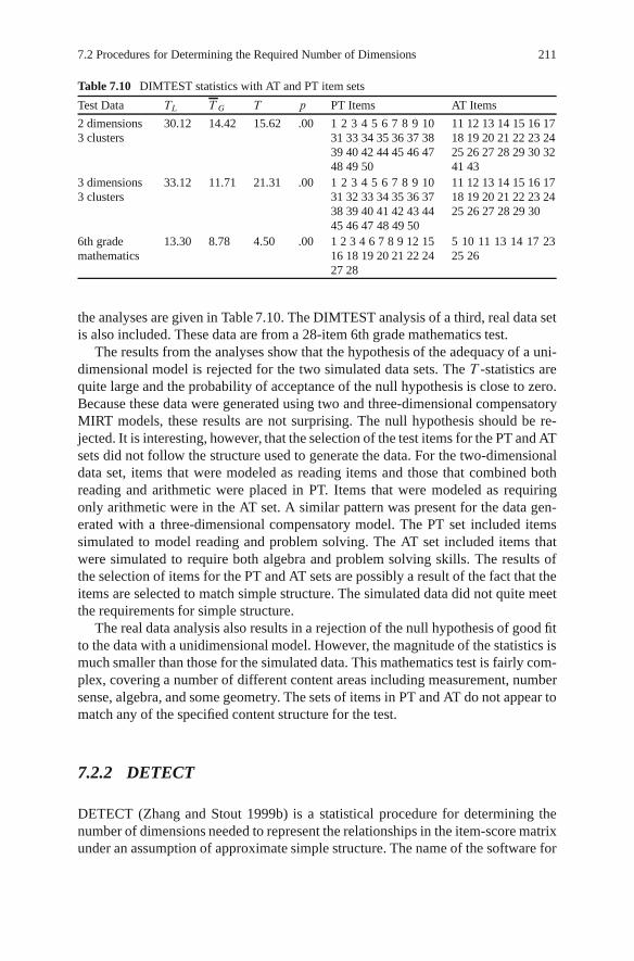
7.2 Procedures for Determining the Required Number of Dimensions 211
Table 7.10 DIMTEST statistics with AT and PT item sets
Test Data TL T G T p PT Items AT Items
2 dimensions3 clusters
30.12 14.42 15.62 .00 1 2 3 4 5 6 7 8 9 1031 33 34 35 36 37 3839 40 42 44 45 46 4748 49 50
11 12 13 14 15 16 1718 19 20 21 22 23 2425 26 27 28 29 30 3241 43
3 dimensions3 clusters
33.12 11.71 21.31 .00 1 2 3 4 5 6 7 8 9 1031 32 33 34 35 36 3738 39 40 41 42 43 4445 46 47 48 49 50
11 12 13 14 15 16 1718 19 20 21 22 23 2425 26 27 28 29 30
6th grademathematics
13.30 8.78 4.50 .00 1 2 3 4 6 7 8 9 12 1516 18 19 20 21 22 2427 28
5 10 11 13 14 17 2325 26
the analyses are given in Table 7.10. The DIMTEST analysis of a third, real data setis also included. These data are from a 28-item 6th grade mathematics test.
The results from the analyses show that the hypothesis of the adequacy of a uni-dimensional model is rejected for the two simulated data sets. The T -statistics arequite large and the probability of acceptance of the null hypothesis is close to zero.Because these data were generated using two and three-dimensional compensatoryMIRT models, these results are not surprising. The null hypothesis should be re-jected. It is interesting, however, that the selection of the test items for the PT and ATsets did not follow the structure used to generate the data. For the two-dimensionaldata set, items that were modeled as reading items and those that combined bothreading and arithmetic were placed in PT. Items that were modeled as requiringonly arithmetic were in the AT set. A similar pattern was present for the data gen-erated with a three-dimensional compensatory model. The PT set included itemssimulated to model reading and problem solving. The AT set included items thatwere simulated to require both algebra and problem solving skills. The results ofthe selection of items for the PT and AT sets are possibly a result of the fact that theitems are selected to match simple structure. The simulated data did not quite meetthe requirements for simple structure.
The real data analysis also results in a rejection of the null hypothesis of good fitto the data with a unidimensional model. However, the magnitude of the statistics ismuch smaller than those for the simulated data. This mathematics test is fairly com-plex, covering a number of different content areas including measurement, numbersense, algebra, and some geometry. The sets of items in PT and AT do not appear tomatch any of the specified content structure for the test.
7.2.2 DETECT
DETECT (Zhang and Stout 1999b) is a statistical procedure for determining thenumber of dimensions needed to represent the relationships in the item-score matrixunder an assumption of approximate simple structure. The name of the software for

212 7 Analyzing the Structure of Test Data
this procedure, DETECT, is an abbreviation for “dimensionality evaluation to enu-merate contributing traits.” DETECT has the same theoretical basis as DIMTEST.The procedure does not assume any specific form for the item characteristic func-tions so it is labeled as a nonparametric procedure. Although the desire is to knowthe number of coordinate dimensions needed to model the data matrix assuming aspecific model, DETECT is often used for this purpose so its statistical underpin-nings are described here and the method is applied to the two example data sets todemonstrate its use.
The DETECT methodology is based on several assumptions for the character-istics of the probabilistic models that generate the item-score matrix. With oneexception, these are the usual assumptions that were made in describing the MIRTmodels for dichotomously scored items in Chap. 4. They are that the item responsefunctions are monotonically increasing with an increase in any of the �-coordinatesand that local independence holds when determining the probability of a stringof item scores conditional on ™ from the probabilities of each item score condi-tional on ™. The assumption that was not included in Chap. 4 is that the procedureis based on “pairwise local independence” instead of complete local indepen-dence. Pairwise local independence specifies that the following conditions hold:cov
�Ui; Uj j‚ D ™
D 0 for all ™ and i ¤ j , where i and j represent item numbersin the test. This definition of local independence is consistent with the estimationused in NOHARM, but TESTFACT uses the full probabilistic definition of localindependence.
The basic definition of dimensionality used in the development of DETECT isthat an item-score matrix requires a d -dimensional model for accurate represen-tation of the relationships in the matrix if d is the minimum number of elementsrequired in the ™-vector to produce pairwise local independence using a mono-tonically increasing MIRT model. When the ™-vector results in pairwise localindependence, the model is labeled as “complete.”
Conceptually, the DETECT method searches for homogeneous clusters of itemsthat best measure in a direction in the multidimensional space that is different thanthe direction of best measurement for the test as a whole. The direction of best mea-surement for the test is somewhat similar to the concept of the reference compositedescribed in Chap. 5, but its mathematical definition is not the same. The major dis-tinction is that the reference composite is an estimate of the direction through theorigin of the ™-space that corresponds to the weighted composite of coordinates thatresult from the application of a unidimensional IRT model to the item score matrix.In contrast, the direction of best measurement used in DETECT is the average di-rection over ™-points that give the greatest change in estimated true score for the setof test items. The derivation of this direction is given in Zhang and Stout (1999a).A short summary is provided here.
The basic concept for the DETECT index is a weighted composite of the �-coordinates for the complete latent space. The weighted composite is defined asfollows
�w D w™0 DmX
kD1wk�k; (7.24)

7.2 Procedures for Determining the Required Number of Dimensions 213
where w is a vector of weights for them coordinates in the space and �w is the valueof the composite of the coordinates. The weights are scaled so that the variance of�w is equal to 1.0.
The DETECT procedure determines the values of the elements of the vector wthat maximize the expected value over the ™-space of the square root of the in-formation function in the direction specified by the composite. w� is the vector ofweights that provide the maximum expected value. The estimation equation for theelements of w� is given by
w� D c
kX
iD1E
8<
:
@Pi .™/
@�`
"kX
ID1PI .™/QI .™/
#� 12
9>=
>;for ` D 1; 2; : : :; m; (7.25)
where w� is an element of w�, c is a scaling constant to result in a variance of 1 for�w, k is the number of items on the test, Pi.™/ is the item response function for Itemi , and m is the number of dimensions needed to model the relationships in the datamatrix.
To implement DETECT, the set of items in a test is first partitioned into a seriesof disjoint sets, P D ˚
A1; A2; : : : ; Aq�
with the goal of having items in the differentsets measuring different constructs. These sets can either be determined by the judg-ment of the test developer, or DETECT provides an option to find the partition thatmaximizes the value of the DETECT index. The DETECT index,Dw.P/, is given by
Dw .P/ D 2
k.k � 1/
X
1�i�j�kıij .P/ E
�Cov
�Ui ; Uj j�w
�; (7.26)
where P is any partition of the items in the test, k is the number of items on the test,i and j are any two items on the test with corresponding scores Ui and Uj , �w isthe composite of interest, and
ıij .P/ D(1 i; j 2 A`�1 otherwise:
(7.27)
That is, the ı function assigns 1 if two items are in the same partition of the testand �1 if they are in different partitions. When the composite is based on optimalweights, the index is denoted as D.P/ and it is called the theoretical DETECTindex for partition P. The partition that maximizes the index is labeled P�. In theimplementation of the DETECT index in the software, the value given by (7.26) ismultiplied by 100 (Roussos and Ozbek 2006). The range of values for the in-dex that are typically observed are 0 to positive values less than five. Jang andRoussos (2007) give the following guidelines for interpreting the DETECT index
“An index value of 1 or more is considered to indicate large multidimensionality(Kim, 1994). Values of .4 to 1 are considered to indicate moderate to large multidimension-ality. Values below .4 are considered to indicate moderate to weak multidimensionality, oreven unidimensionality for values below .2.” (p. 7)

214 7 Analyzing the Structure of Test Data
Along with the DETECT index, the software provides two other indicators ofthe dimensionality of the data. The first is based on a cross-validation of DETECTindex. The data matrix is randomly divided into two samples. The partition that max-imizes (7.26) is determined for the first sample. The value of D.P�/ for that sampleis labeledDmax. The partition that maximizes the second sample is also determined.Then D.P/ is computed using the data from the first sample using the partition de-termined from the second sample. This value is called the reference DETECT indexand it is labeled Dref. The ratio of these two values Dref=Dmax is considered asanother index of dimensionality. If the value is near 1, it means that the partitionsfound from the two samples are the same indicating that the solution is stable. If theratio is small, it means that the partitions are very different. Zhang and Stout (1999b)suggest that small values of the ratio indicate that the partitions are based on “capi-talization upon chance” and likely indicate essential unidimensionality.
The other indicator of dimensionality is the proportion of estimated covariancesthat have signs that follow the pattern that is expected by the partitioning of the testinto item sets. The expected pattern is that items within the same partition shouldhave positive covariances, but those in different partitions should have negative co-variances. This indicator is called the IDN index. Values close to 1 indicate that thepattern of covariances matches the pattern that is expected if the multidimensionalstructure of the data is consistent with a simple structure model.
The DETECT analysis was performed on the same data sets as were used withthe DIMTEST method – the two simulated data sets and the real data from themathematics test. For the simulated data, the program was run in two different ways.The first was using the exploratory mode with DETECT identifying the partition ofitems that maximized the DETECT index. The second was a confirmatory analysisusing the partition of test items into clusters according to the way that the data weregenerated. The results of these analyses are presented in Table 7.11.
The interpretation of the DETECT index suggests that the two- and three-dimensional data sets have moderate to large multidimensionality, as would beexpected given how they were generated, but the real data set has weak dimensional
Table 7.11 DETECT results for the three example data sets
Data set Cross-validatedDETECTindex
RatioDref=Dmax
IDNindex
Partition
1 2 3
2 dimensions3 clusters
.50 .73 .74 1–10,32–40, 42,44–50
11–30, 41,43
31
3 dimensions3 clusters
.72 .86 .83 1–10, 31–50 11–30
6th grademathematics
.18 .41 .66 1, 2, 15–19 3, 4, 6–9,12, 20–22,24, 27, 28
5, 10, 11,13, 14, 23,25, 26

7.2 Procedures for Determining the Required Number of Dimensions 215
structure or support for modeling with a unidimensional model. This is the casefor the real data, even though the hypothesis of unidimensionality was rejected byDIMTEST.
The ratios of the DETECT indexes are fairly close to 1 for the simulated datasets indicating stable solutions, but the real data set yielded a smaller ratio of .41suggesting some instability in the solution. The IDN Index is largest for the three-dimensional data and smallest for the real data set. The results give a clear indicationthat the real data is more likely to be adequately modeled with a unidimensionalmodel than the other two data sets. This is not a surprising result because the itemsfor the real test were partly selected based on the item-total test correlation. Use ofthis selection criterion tends to result in a dominant construct for a test, even thoughthere are multiple content areas. In this case, the test is equated using a unidimen-sional IRT model so the DETECT results support the use of that methodology.
DETECT also gives information on the partitioning of the test items into subsetsthat maximizes the DETECT Index. In this case, the methodology suggested threeclusters of items for the two-dimensional case, but the clusters do not correspond tothe structure built into the data. For the three-dimensional case, DETECT suggestedtwo-item clusters rather than the three built into the data. The mismatch between theactual and estimated item clusters is due to the fact that DETECT tends to ignoreitems that are along the reference composite for the test and it is trying to fit an inde-pendent, simple-structure model. For the simulated data, the method combined theitem sets that had high a-parameters on a dimension, even though some of the itemsalso had high a-parameters on other dimensions. It is only when the test items withhigh a-parameters formed disjoint sets with no contribution from other dimensionsthat the method correctly clusters items.
The partitioning of the test items for the real test is more difficult to interpretbecause the true underlying structure is not known. There are content classificationsfor the items, but there is only a partial match between the content classifications andthe partitioning of the items from DETECT. For example, the first partition has fouritems that had content classifications of measurement, but three other items with thesame classification were in the other two partitions. There was no strong connectionbetween the content classifications by the test developers and the partitions producedby DETECT.
7.2.3 Parallel Analysis
Another approach to determining the number of dimensions is called parallel anal-ysis. The approach has been suggested by Ledesma and Valero-Mora (2007) andothers. It has a long history in the factor analysis literature possibly being first sug-gested by Horn (1965). The procedure has two major steps. First, a dimensionalanalysis is performed with a program like TESTFACT that provides the first n eigen-values of the matrix of inter-item correlations. TESTFACT bases its eigenvalues/eigenvector decomposition on tetrachoric correlations that may have been adjusted

216 7 Analyzing the Structure of Test Data
using the estimate of the lower asymptote for the item characteristic surfaces forthe items. The eigenvalues can then be plotted against the number of dimensionsextracted to give the traditional scree plot.
The second step is to generate a set of test data that has no relationship amongthe items, but that has the same proportion correct for each item as the real data andthe same sample size. The generated data are then analyzed to get eigenvalues usingthe same analysis as was applied to the real data. Because the generated data have thesame distribution of item difficulties as the real data, the analysis of these data willhave the same tendency to have difficulty factors as the real data. The eigenvaluesfor the generated data are then plotted on the same graph with the correspondingones from the real data and the number of eigenvalues for the real data that arelarger than those for the generated data is determined. That number is the numberof dimensions suggested by the analysis. Ledesma and Valero-Mora (2007) suggestreplicating the generation of the simulated data that matches the difficulty values forthe real data a number of times to get an estimate of the sampling variation of theeigenvalues for the sample size and difficulty distribution from the real data.
To demonstrate the parallel analysis methodology, it was applied to the three datasets described earlier in this chapter – the two simulated data sets and the one realdata set. First, TESTFACT was run on each data set to obtain the eigenvalues foreach of the dimensions extracted. Next, the proportion correct was computed foreach test item from the item-score matrix. The proportion correct was then usedas the parameter of a binomial distribution and random binary digits were gener-ated to match that proportion using the binomial random variable generator fromMATLAB. The result is a matrix of random .0; 1/ data that has the same diffi-culty distribution as the original data. These random data were then analyzed withTESTFACT to obtain the eigenvalues from the tetrachoric correlation matrix. Forthe real data, TESTFACT was run with lower asymptote parameters estimated us-ing BILOG-MG.
The results for the two-dimensional simulated data set are shown in Fig. 7.8 andthose for the three-dimensional data set are shown in Fig. 7.9. The solid line in eachfigure is the scree plot for the multidimensional data and the dotted lines are thescree plots for the random data.
The scree plot shows that the first two eigenvalues for the two-dimensional datawere larger than the first two eigenvalues for the random data. There was verylittle variation in the random data so a larger number of replications were not per-formed. There was one anomaly in the random data. One replication had three ofthe tetrachoric correlations that did not converge to stable values. Arbitrary valueswere substituted for those values and they resulted in the two eigenvalues from therandom data that were approximately 2. The rule proposed by Ledesma and Valero-Mora (2007) was that the number of dimensions needed to model the data is thenumber of eigenvalues that are greater than those from the random data. In thiscase, the rule results in two dimensions. This is the number of dimensions used togenerate the data. It is not the number of item clusters used to generate the data,which was three. It is interesting to note that the eigenvalues greater than one rulewould result in the retention of over 20 dimensions for this data set. That rule is notvery useful for these data.

7.2 Procedures for Determining the Required Number of Dimensions 217
0 5 10 15 20 25 30 35 40 45 500
2
4
6
8
10
12
Factor Number
Eige
nval
ue
Fig. 7.8 Scree plot for the two-dimensional simulated data and four replications of random data
0 5 10 15 20 25 30 35 40 45 500
2
4
6
8
10
12
Factor Number
Eige
nval
ue
Fig. 7.9 Scree plot for the three-dimensional simulated data and two replications of random data
Figure 7.9 shows the scree plot for the three-dimensional simulated data andFig. 7.10 shows the plot for the real data set. For the three-dimensional data, thefirst three eigenvalues from the three-dimensional data exceeded the correspondingeigenvalues from the random data. As for the data generated using two dimensions,the parallel analysis methodology correctly identified the number of dimensions. Inthis case, only two random data sets were generated to serve as a basis for compari-son because the scree plots for those two data sets were nearly identical.

218 7 Analyzing the Structure of Test Data
0 5 10 15 20 25 300
1
2
3
4
5
6
7
8
9
10
Factor Number
Eige
nval
ue
Fig. 7.10 Scree plots for the grade 6 mathematics test data and three replications of random data
The real data consisted of the item score matrix of the response of 6,000 studentsto 28 multiple-choice test items. The c-parameters for the items were first estimatedusing BILOG. The c-parameters ranged in value from .09 to .36. The c-parameterestimates were set as fixed values in TESTFACT. The scree plots for the real data setand two randomly generated data sets are shown in Fig. 7.10. The scree plot for thereal data is shown with a solid line and those for the simulated data are shown withdotted lines. Only two replications were used for the simulated data because the linesfor the replications were indistinguishable indicating there was little variation in theresults of the simulation. The first two eigenvalues for the real data were larger thanthose for the simulated data sets suggesting that modeling the data using a ™-spacewith two coordinate axes would capture the relationships between the item scoresin the data matrix.
7.2.4 Difference Chi-Square
Schilling and Bock (2005) suggest using a 2 test of the difference in fit of modelswith m and m C 1 dimensions to determine the number of coordinate axes neededto model the relationships in the item response matrix. Tate (2003) selected this 2
difference test as one of the methods for evaluation in research on model fit and hegenerally found that it worked well.
The procedure for implementing the 2 difference test is to run TESTFACT onthe item response matrix specifying m and then m C 1 dimensions. For each ofthe solutions, the 2 goodness of fit statistic is computed. There is some questionwhether this fit statistic really has a 2 sampling distribution, but the difference in

7.2 Procedures for Determining the Required Number of Dimensions 219
the fit statistics has been shown to have a 2 sampling distribution (Haberman 1977).Therefore, the difference in the 2 values for the successive solutions is calculated aswell as the difference in the degrees of freedom for the two 2 values. The resultingdifference in 2 statistics is tested as a 2 statistic with degrees of freedom equalto the difference in degrees of freedom for the two values. The expression for thedifference in 2 values as presented in Schilling and Bock (2005) is given in (7.28),
2 D 2
sX
`D1r` log OP` � 2
sX
`D1r` log OP 0; (7.28)
where 2 is the 2 difference statistic, s is the number of observed response stringsin the observed item score matrix, r` is the frequency of observing response string `,OP` is the marginal probability of response string ` estimated withm dimensions, andOP 0 is the marginal probability of response string ` estimated withmC1 dimensions.
The degrees of freedom for the difference 2 is the number of items in the test, n,minus the number of dimensions, n �m.
The 2 difference statistic was computed for the simulated and real data usedwith the previous methods. The results of the statistical test of the null hypothesisthat the additional dimension provides no improvement in fit are given in Table 7.12for the two simulated and one real data set. When the 2 difference is statisticallysignificant, it indicates that adding a dimension results in a significant improvementin fit. When the 2 value is not significant at the specified level, the additional di-mension does not result in significant improvement in fit suggesting that the smallerof the two numbers of dimensions is appropriate for analysis.
For the two simulated data set, following the usual convention of rejecting thenull hypothesis when p < :05 results in an over estimate in the number of dimen-sions required to model the data. The two-dimensional data set still has significant
Table 7.12 2 difference test for number of dimensions for the simulated and real data sets
Dimensions tested Data set
2 dimensions 3 dimensions 6th grade3 clusters 3 clusters mathematics
1 vs. 2 2 4005:86 4926:49 181:05
d.f. 49 49 27
Probability :00 :00 :00
2 vs. 3 2 96:90 399:39 117:19
d.f. 48 48 26
Probability :00 :00 :00
3 vs. 4 2 57:64 85:84 28:31
d.f. 47 47 25
Probability :14 :00 :29
4 vs. 5 2 80:13
d.f. 46
Probability :00

220 7 Analyzing the Structure of Test Data
improvement in fit when three dimensions are used. The three-dimensional data sethas significant improvement in fit when analyzed using four or even five dimensions.A review of the a-parameter estimates from the solutions with more than enough di-mensions indicates that a few items were not well estimated when the true numbersof dimensions were used and these items had improved fit with more dimensions.The added dimensions can be considered as resulting from poor estimation. How-ever, if the kind of “rule of thumb” used in structural equation modeling, such asjudging fit as good when the 2 divided by the degrees of freedom is less than threewere used, the use of the difference 2 would recover the number of dimensionsused to generate the data.
The analysis of the real data suggested that two dimensions would be needed tomodel the relationships present in the item score matrix. Even though the 2 dif-ference test supports the need for three dimensions, the results from the analysesof simulated data that show a tendency for the difference test to ever-estimate thenumber of dimensions, the fact that the a-parameters for the third dimension aresmall, and the difficulty of interpreting the construct for the third coordinate suggestthat two dimensions is a better choice. This choice is also consistent with the con-clusion drawn from the parallel analysis of the test. The DETECT results lent somesupport to using only a single dimension for modeling these data. The 2 dividedby degrees of freedom was still much larger than three for all of the numbers ofdimensions considered, so that rule did not seem to be the solution to the number ofdimensions problem.
7.3 Clustering Items to Confirm Dimensional Structure
An approach to determining the number of coordinate axes that are needed to modelthe relationships in the data that is somewhat more subjective than those in the pre-vious section is to perform a cluster analysis of a measure of similarity of theconstructs measured by the items. As shown in the two simulated examples in theprevious section, the number of clusters does not necessarily indicate the numberof coordinate axes needed for the solution. For the two-dimensional simulated data,three item clusters were used to generate the data, but only two coordinates wereused to locate the examinees. The number of item clusters is an upper limit on thenumber of coordinate axes needed, but it may be possible to represent the relation-ships in the data with fewer coordinates per person than the number of item clusters.
One way to use item clusters to determine the number of dimensions that areneeded to model a data set is to compare the results of the cluster analysis for dif-ferent numbers of dimensions. If the cluster analyses are essentially the same fordifferent numbers of dimensions, the smaller of the number of dimensions used forthe analysis is sufficient to model the relationships in the data matrix.
A clustering of items is based on two decisions. The first is the selection of ameasure of similarity between items. The second decision is the algorithm for form-ing clusters. The cluster analysis literature contains a large number of choices forboth of these decisions. Within the MIRT literature, there are two major options

7.3 Clustering Items to Confirm Dimensional Structure 221
for each of these. For the similarity measure, one option is the angle between eachpair of item arrows (Miller and Hirsch 1992). The other measure is the conditionalcovariance between the items given in (7.15).
The clustering method that seems to work well when the angle between items isthe similarity measure is Ward’s method (1963). Kim (2001) evaluated a number ofclustering methods and found that Ward’s method recovered the underlying structureof the data more accurately than alternatives. The DIMPACK V. 1.0 (2006) soft-ware uses the conditional covariances as the similarity measure for identifying itemclusters. The software package does not recommend a particular clustering method.Instead, numerous alternatives are provided. However, Roussos et al. (1998) in-dicate that the unweighted pair-group method of averages (UPGMA) (Sokal andMichener 1958) gave better recovery of clusters in a simulation study than othermethods. The remainder of this section describes the procedure for computing theangle between item arrows and the implementation of Ward’s method for clustering.
If the item arrow for Item 1 has angles with the coordinate axes in vector ’1 andthe angles with the coordinate axes for the item arrow for Item 2 are in arrow ’2,then the angle between the two item arrows is given by the inverse cosine of theinner product of the cosines of the angles with each the coordinate axes for eachitem (Harman 1976, p. 60):
˛12 D arcos�cos ’0
1cos ’2: (7.29)
Note that ˛12 is a scalar value because the lines formed by extending the item arrowsintersect at the origin and two intersecting lines fall within the same plane. Thus,there is only one angle between the two lines extended from the item arrows ratherthan a vector of angles.
The relationship between the angle between two item arrows and the a-parameters for the items can be derived by substituting the expression for thedirection cosines for the items (5.8) into (7.29). That is,
cos˛12 D a01s
mP
`D1a21`
a2smP
`D1a22`
: (7.30)
If the two item arrows are perfectly aligned with each other, the angle betweenthem will be 0ı. As the angle between the item arrows increases, the items have theirdirections of maximum discrimination in different directions in the ™-space. Forcognitive test items, the angles between items seldom exceed 90ı. Harman (1976,p. 63) shows that the cosine of the angle between two variables, in this case, testitems, is the correlation between the two items. The fact that the cosine of 0ı is 1 in-dicates that, when the item arrows are pointing in the same direction, the continuouslatent variables assumed to underlie the performance on the items are perfectly cor-related. Item arrows pointing at right angles to each other indicate a zero correlationbetween the underlying latent variables. The input data for the clustering algorithmis the matrix of angles between all possible pairs of test items.

222 7 Analyzing the Structure of Test Data
Table 7.13 Angles in degrees between selected test itemsfrom Example B for two and three-dimensional analyses
Item number Item number
1 2 11 12 31 32
1 6:0 82:6 81:7 37:9 33:6
2 10:4 76:6 75:7 31:9 27:6
11 81:9 76:1 :9 44:8 49:0
12 79:7 74:5 3:8 43:8 48:1
31 42:1 33:6 44:7 44:0 4:2
32 44:0 34:2 50:1 50:1 9:8
For the examples used in this chapter, the matrices are too large to fit on a page.50 � 50 or 30 � 30/ so they are not presented here. A few examples of angles be-tween item pairs are provided in Table 7.13. The item pairs used here are fromExample B used earlier in this chapter. For the example, pairs of items have been se-lected from each set that is best at measuring a different reference composite: items1 and 2, 11 and 12, and 31 and 32. In Table 7.13, the numbers above the diagonalgive the angles between item pairs from a two-dimensional solution for the data andthose below the diagonal are from a three-dimensional solution.
The results in Table 7.13 show that the items that have highest discriminationfor the same construct have small angles between the item arrows. The largest ofthese is 10 degrees. The angles between items that are best at measuring differentconstructs have much large values, for example 82:6ı between Items 1 and 11. Novalues are given in the diagonal of the table because this would be the angle betweenan item and itself, which is 0. The angles below the diagonal are slightly larger thanthose above the diagonal. For example, all of the angles with Item 32 in the three-dimensional solution are larger than the corresponding angles with Item 32 in thetwo-dimensional solution. The differences are not great because this example doesnot have item arrows that project on top of each other when the lower dimensionalsolution is used. The small differences suggest that although the clustering of itemsbased on the angle between item vectors is useful for investigating dimensionality,this type of analysis does not give conclusive information about the required numberof dimensions. It is only when there is a major difference in the solution that it isclear that it means that the higher number of dimensions is needed.
The cluster analyses dendrograms for the two examples are shown in Fig. 7.11.The upper panel gives the results for the three constructs in two dimensions and thelower panel gives the corresponding results for the three constructs in three dimen-sions. In both cases, the three sets of items are clearly and accurately identified. Thisis in contrast to the results from DETECT presented in Sect. 7.2.2 where only twoclusters were identified for the case with three constructs in three dimensions.
The vertical axes in Fig. 7.11 are a function of the sum of the squared distancebetween the items in one cluster and those in another. The values on the axes cannot be directly converted into an angle measure. For example, in the lower panel, theaverage angle between the items with numbers 1 – 10 and those with item numbers

7.3 Clustering Items to Confirm Dimensional Structure 223
1418111921281725123020291516132324222627 1 7 9 5 8 2 6 3 4 1031483537365033473445464438493940423241430
50
100
150
200
Roo
t Mea
n Sq
uare
Dev
iatio
nExample A
2 5 6 8 9 1 10 3 4 7 313544344743463245394249363738334050414811152219121318272914161724302023282125260
50
100
150
200
250
Example B
Item Number
Roo
t Mea
n Sq
uare
Dev
iatio
n
Fig. 7.11 Dendrograms for cluster analyses of Examples A and B
from 31 to 50 is about 40ı, but the connecting line between the two item clusters isat 165.4. That value depends on the squared angles and the number of items in thecluster.
The results of a clustering of the angles between test items on a real test cannotbe expected to be as precise as those from simulated data. The clusters from thetwo-dimensional solution of the grade 6 mathematics test are given in Fig. 7.12.
The results in Fig. 7.12 show that there is a fairly clear clustering of the items inthe test, but that the clustering does not match well with the subjective classificationof test items by content. With the exception of the items labeled “D”, Data Anal-ysis and Probability, the single content areas do not fall within a distinct cluster.The other content areas are “M”, Measurement, “G”, Geometry and Spatial Sense,“N”, Number Sense and Numeration, and “P”, Patterning and Algebra. A detailedanalysis of the content of the items might give a better explanation for the clustering.Better yet would be information from the students about how they approached each

224 7 Analyzing the Structure of Test Data
M G N M G P D D D M D P D P N N P M M N M N N G P G P M0
10
20
30
40
50
60
70
80
Item Classification
Roo
t Mea
n Sq
uare
Dev
iatio
n
Fig. 7.12 Dendrogram for clustering of grade 6 mathematics test items
test item. This clustering is based on the similarity of the way in which studentsresponded to the items. The way that students approach the items might not be thesame as the way that the persons writing the items intended.
The angles between the items in the two major clusters tend to be about 30ı to50ı apart. This amount of separation corresponds to correlations between referencecomposites of .6 or .7. This level of correlation is not surprising for the contentwithin a mathematics test. It would be expected that students would learn all of thecontent together as part of the classroom instruction. Within the clusters, the anglesbetween items are much smaller, usually varying from almost perfect alignment indirection to a few degrees between the item vectors. The results support reportingthree or four subcontent areas within the test, but they do not seem to match up withthe content classifications supplied by the writers of the test items.
7.4 Confirmatory Analysis to Check Dimensionality
The analysis procedures described in previous sections were exploratory in the sensethat directions of best measurement of test items were not specified in advance ofdoing the analysis. The DIMTEST and DETECT procedures do allow prespecifica-tion of test items to clusters yielding a check on how well the data in the item-scorematrix conform to the hypothesized structure. Other programs such as NOHARMand ConQuest provide options for either fixing parameters at specified values orindicating which a-parameters should be set to zero. These confirmatory proce-dures are often used to check hypotheses of a dimensional structure when a test

7.4 Confirmatory Analysis to Check Dimensionality 225
has been designed to measure specific constructs. The simulated test in Example Aof Sect. 7.2 is used here to demonstrate the confirmatory approach using the NO-HARM software. Recall that this simulated test had three clusters of test items, butthe clusters can be represented in a two-dimensional coordinate system.
Because there are three specific item types in the test, an initial confirmatoryanalysis might be to specify each of the item sets as defining a construct and hy-pothesizing a three-dimensional orthogonal coordinate system with each item setaligned with one of the coordinate axes. That means that the confirmatory analysiswill set two of the a-parameters for each item to 0 and allow one to be nonzero. Thecorrelation between the coordinates for the persons would also be set to zero and theunits for the dimensions would be fixed by setting the standard deviations of eachof the coordinates to 1.0.
The results of that analysis resulted in a sum of squared (SS) residuals of .06 anda root mean square of residuals (RMSE) of .0211. These measures of fit might seemsmall, but they are averages over 1225 values in the lower diagonal of product mo-ment matrix and the averaging may hide some clusters of relatively high residuals.As a formal hypothesis test of whether the residuals are from a MIRT model that fitsthe data, Gessaroli et al. (1996) developed an approximate 2 test of fit. Their proce-dure converts the residual matrix from the NOHARM output into estimated residualcorrelations and then converts those correlations to z-scores using the Fisher r to ztransformation. Finally, these z-scores are squared and summed over the lower di-agonal matrix. The result is a 2 distributed fit measure with degrees of freedomequal to 1=2 I .I � 1/ � t , where I is the number if test items in the analysis andt is the number of independent parameters being estimated. In the current example,the number of test items is 50 and the number of parameters being estimated is onea-parameter per item and one d -parameter per item, so t D 100. The total degreesof freedom is 1; 225� 100 D 1; 125.
The 2 value for this initial confirmatory analysis of the data was very large(see Table 7.14) so it seems logical to free some parameters to improve the fit. Theclusters of items might not be orthogonal to each other so allowing nonzero cor-relations among the coordinates seems to be a good next step in the confirmatoryanalysis. The results for the solution with correlated coordinates are a substantialimprovement over the orthogonal solution. The SS residuals and RMSE are much
Table 7.14 Fit measures for successive models of the two-dimensional, three-clustersimulated data
Analysis model
3d orthogonal 3d oblique 2d orthogonal 2d oblique
2 55,697 1410 4056 1264df 1125 1122 1105 1104p .00 .00 .00 .00 2/df 49.51 1.26 3.67 1.15SS .06 .02 .04 .01RMSE .021 .004 .006 .003

226 7 Analyzing the Structure of Test Data
smaller than the three-dimensional orthogonal solution and the 2 value is muchsmaller as well. The significance level for the 2 statistics still indicates that theresiduals are significantly larger than those for a perfectly fitting model, but the 2
divided by the degrees of freedom is 1.26, a value that would be considered as goodfit in the structural equation model literature. Overall, this three dimensional solu-tion might be considered as doing a good job of representing the relationships in thedata and this solution might be accepted. The only part of the result that might raisesome further questions about the appropriateness of the three dimensional model isthe high intercorrelations between the coordinates on the third dimension and thosefrom the other two dimensions. The correlations between the coordinates are given
in the correlation matrix
2
41 :30 :78
:30 1 :82
:78 :82 1
3
5.
Because the correlations of the coordinates for the third dimension were so highwith the other two dimensions, the items assumed to measure that dimension wereallowed to have nonzero a-parameters on the other two dimensions. First, this wastried with the constraint that the coordinates were uncorrelated. This is the “2d or-thogonal” column of the table. These results were worse fitting than the “3d oblique”solution but better than the “3d orthogonal” solution. Because relaxing the constrainton the correlation between coordinates improved fit when specifying three dimen-sions, the same approach was taken for two-dimensions. These results are given inthe last column of the table and the give slightly better fit than the “3d oblique”solution.
The fit of the two cases with correlated coordinates is so close that either couldbe considered as acceptable models for the data. Because the data were generatedassuming two-dimensions, this demonstrates a point made in an earlier chapter thatdata that are well modeled in m dimensions can always be well modeled in m C 1
dimensions.Confirmatory analyses seldom have the luxury of knowing the correct solution
as a means of judging the quality of the result. A more realistic example of the con-firmatory approach is shown here using the data from the sixth grade mathematicstest that was analyzed using cluster analysis earlier in this chapter (see Sect. 7.3 andFig. 7.12). This test was constructed to cover material from five content domains.Therefore, a logical first confirmatory analysis might be to hypothesize that eachof the five content domains measure orthogonal components. For the analysis, eachitem was constrained to have a nonzero a-parameter on one coordinate dimensionand zero values on all others. The correlations between the coordinates for the lo-cations of the examinees were also fixed at zero. The results for the NOHARManalysis using this set of constraints are given in Table 7.15. The results show poorfit using all criteria.
A logical next step might be to remove the constraints on the correlations. Itseems unlikely that a test of mathematics would have zero correlations betweennumerical computation skill and a data analysis skill, for example. This analysisallowing correlated coordinates dramatically improves the fit of the model to the

7.4 Confirmatory Analysis to Check Dimensionality 227
Table 7.15 Fit measures for successive models of the two-dimensional, three-cluster simulateddata
Analysis model
5d orthogonal 5d oblique 4d oblique 3d oblique 4d clusters
2 48,298 735.92 735.84 759.55 616.04df 322 312 316 319 316p 0 0 0 0 0 2/df 150.00 2.35 2.33 2.39 1.95SS .405 .0057 .0057 .0059 .0049RMSE .0327 .0039 .0039 .0039 .0036
data. The results of this analysis are presented in the second data column ofTable 7.15. Although the fit is very good for this confirmatory analysis, the esti-mated correlations between coordinates were very high and one estimate betweenthe first and third coordinate was 1.002. A conclusion form these results might bethat the first two content domains were measuring essentially the same set of skillseven thought they were labeled “Measurement” and “Number Sense and Numer-ation.” To check this hypothesis, another confirmatory analysis was run with theitems from these two content categories coded to be measuring the same dimensionyielding a four dimensional model. Correlations between the coordinates remainedunconstrained.
The results for the four dimensional solution are also given in Table 7.15. Thefit of this model is essentially the same as that for the five-dimensional modelindicating that there was no reduction in the recovery of the relationships in thedata. The correlations between the coordinates for the four-dimensional modelwere also very high, but none reached the level of 1.00. The correlation matrix is2
664
1 :93 :88 :92
:93 1 :90 :96
:88 :90 1 :93
:92 :96 :93 1
3
775. To check if an even simpler model might be appropri-
ate, the test items for the second and forth dimensions were combined into a singleset to produce a three-dimensional confirmatory solution. This model had slightlyworse fit than the four-dimensional model. This supports a conclusion that the four-dimensional model is the best of those considered.
There is always a concern when doing confirmatory analyses of matrices of itemresponse data that the results are dependent on the subjective judgments of those do-ing the classification of items into content categories. Those classifications are basedon the expert judgments of content experts and those individuals might not approachthe test items in the same way as a 6th grade student. As a basis for comparison, theconfirmatory analysis was repeated using the results of the cluster analysis for thedata shown in Fig. 7.12. The items were classified into four clusters based on the di-agram. These fit statistics for this model are shown in the last column of Table 7.15.The fit of the confirmatory model based on the cluster analysis is notably better

228 7 Analyzing the Structure of Test Data
than that for the four-dimensional solution based on the subjective classifications ofitems into clusters. This is not a surprising result because the clusters were based onthe same set of data that was used for judging fit. It does raise some concerns aboutthe judgmental classification of test items into content categories. It is wise to lookfor support for the validity of the classifications using some exploratory analyses orother sources of evidence.
7.5 Concluding Remarks
This chapter presents a conceptual framework for considering the problem of de-ciding on the number of dimensions needed when analyzing the matrix of itemresponses. The number of dimensions is considered to be the same as the number oforthogonal coordinate axes and not the number of constructs assessed by a test. Thenumber of constructs is the number of reference composites defined by meaningfulclusters of test items in a test. These clusters of test items should have character-istics that result in close approximations to the requirements for coherence. Froma practical perspective, the number of coherent sets of test items also indicates thenumber of meaningful subscores that can be provided for the test. Of course, forsubscores to be useful, the locations of persons along the continua defined by thecorresponding reference composites must be determined with a sufficient degree ofaccuracy or reliability. Generally, the number of coordinate axes needed to describethe structure of the data from the interaction of persons with the test items is lessthan or equal to the number of coherent item sets in the test. The number of coordi-nate axes is less then the number of coherent item sets when the directions for thereference composites based on some test item sets fall within the same plane.
Along with providing a conceptual framework, this chapter describes a numberof methods for deciding on the number of coordinate axes needed to represent therelationships in the data matrix. The recommended approach is to first determine ifthe hypothesis that the data can be modeled with a unidimensional item responsetheory model is rejected. DIMTEST is a good procedure for testing this hypothesis.If the hypothesis is rejected, then there are a number of procedures for determin-ing the number of coordinate axes (e.g., the number of �s to estimate) for furtheranalysis. In general, it is somewhat better to slightly overestimate the number ofcoordinate axes rather than underestimate them because of the danger of projectingitem sets and person locations into the same location when in reality they differ inimportant ways. The price for overestimating the number of coordinate axes is anincrease in the amount of estimation error.
The final section of the chapter describes a method for identifying the coherentsets of items using cluster analysis. Research on clustering procedures has beenpromising, but much more needs to be done in this area. There are many clusteringmethods and there are even more measures of the similarity of items. It is likely that

7.6 Exercises 229
these methods will be refined in the future. However, use of the methods describedin this chapter should give fairly good information about the functioning of the itemson a test.
7.6 Exercises
1. Fifty sets of random data were simulated to have the same proportion correctfor each test item as a real data set. Then each data set was analyzed using principalcomponents and the eigenvalues were obtained. The mean and standard deviation ofthe first through fifth eigenvalues for the simulated data were computed. The eigen-values for the real data set were also obtained using principal components analysis.The results are presented in the table below. Given this information, how many di-mensions should be used to calibrate the test items using a multidimensional itemresponse theory procedure? Explain your answer.
Component Eigenvalues Mean Eigenvalues Standard deviationnumber from the real from the simulated data of Eigenvalues
data from the simulated data
1 9.1 1.25 .072 2.3 1.20 .063 1.5 1.15 .054 1.1 1.10 .065 .9 1.05 .05
2. A group of individuals are distributed exactly along a line in three-dimensionalspace. The line has the following angles in degrees with the coordinate axes: 65.91,54.74, 45. The line runs through the origin of the three-dimensional space and thedistribution of the individuals along that line is normal with mean 0 and standarddeviation 1. What are the distributions of the coordinates of the individuals for eachof the coordinate axes? What is the correlation between the three coordinates for theindividuals? Show the correlation matrix for the three coordinates.
3. A psychometrician is interested in determining whether the matrix of item re-sponse that was obtained from administering a test to 5,000 individuals can beadequately fit by a unidimensional IRT model. The psychometrician used theDIMTEST program to check for significant violations of the unidimensionality as-sumption. The TL statistic for the matrix of responses was 30.1. The test statisticwas also computed for 100 matrices of simulated data of the same size. The meanvalue of those 100 replications was 14.4. What is the final test statistic for check-ing whether the unidimensionality assumption has been violated? What does thisstatistic say about the assumption of unidimensionality for the analyses of this datamatrix?

230 7 Analyzing the Structure of Test Data
4. All of the test items in a test require capabilities on three distinct, but correlatedconstructs to answer them correctly. The item-score matrix from the test was an-alyzed with a unidimensional IRT model and three of the examinees’ �-estimatesare: 2.58, �:87 and �1:54. The reference composite for this test has angles withthe coordinate axes of 67.6, 52.1, and 46.3 respectively. If all three of these exami-nees fall exactly on the reference composite, what are there coordinates in the threedimensional coordinate system?
5. What is the logical progression that is suggested for determining the number ofcoordinate dimensions needed to model the relationships in a matrix of item scores?What is the difference between non-parametric and parametric procedures used todecide of the number of coordinate dimensions for an analysis?
6. What is the required first step when using the DETECT procedure for determin-ing the number of coordinate axes to use in an analysis? Suppose that you plan toanalyze the data from a 30-item test of knowledge of world geography. How wouldyou implement this first step?
7. Develop your own example of a case where the number of item clusters is greaterthan the number of coordinate axes needed to model the data accurately. Explainwhy fewer coordinate axes than item clusters is adequate for this case.
8. Consider the following variance/covariance matrix:
2
4:1670 :2362 :2892
:2362 :3340 :4091
:2892 :4091 :5010
3
5.
Determine the correlation matrix that corresponds to this variance/covariance ma-trix. What can you infer about the number of coordinate axes needed to uniquelyidentify the locations of individuals whose coordinate vectors were used to generatethis matrix?
9. Table 7.6 shows the correlations between �s used to generate data based on threecoordinates for each examinee and the estimated �s in three dimensions. Note thatthe correlations among the �s used to generate the data are all near 0 and correlationscomputed from the estimates are moderately high. Explain why this is the case.Does the difference in correlations indicate that the TESTFACT analysis does notadequately fit the data? Explain your answer.
10. Explain the meaning of Theorem 2 in a way that would make sense to a personwho has taken only one course in educational testing. What implication does thetheorem have for relating test results from one grade level to the next grade levelwhen the content of the tests changes somewhat?
11. The set of test items shown in Fig. 7.7 requires three coordinate axes to ade-quately model the relationships among them. Give an example of a situation whenthe administration of these test items would result in a matrix of item scores thatcould be well modeled by a unidimensional IRT model. Explain why your examplewould lead to that result.

7.6 Exercises 231
12. Under what circumstances does DETECT tend to underestimate the number ofitem clusters suggested by a matrix of item scores? Describe the characteristics of aset of test items that you believe would result in not identifying a set of test items asbelonging to a cluster.
13. Specify a model and two sets of item parameters that are not equal to each otherthat will make the two sets of items coherent. Show some of the orbits for the twoitems that demonstrate the property of coherence.

Chapter 8Transforming Parameter Estimatesto a Specified Coordinate System
All measurement systems have some arbitrariness to them. When length ismeasured, the size of the unit used is arbitrary. Length units can be chosen from feet,meters, miles, light years, etc. The origin of the length measurements is usually setat true 0 and measurements using different units are typically linear transformationsof each other.1 A common exception is astronomical measurements of distance thatare taken from some arbitrary origin such as the Sun or the center of the Milky WayGalaxy. Although measurements of length are much easier to understand than themeasurements that result from the applications of IRT models, some of the sameconcepts can be used for both types of measurements. For example, the concepts ofinvariance and indeterminacy that are often discussed in the IRT literature also applyto length measurement. The unit of the measurement for length is indeterminate butthe length itself is invariant. The length being measured does not change becausedifferent units of measurement are used, but there is nothing in the measurementof length that indicates that one unit of measurement is more “correct” than anyother unit of measurement. Some units might be more convenient than others suchas using Angstroms when measuring things at the atomic level instead of miles, butthat does not make them more correct.
MIRT models have the same problems of indeterminacy as other measurementsystems. Because of the multidimensional nature of these models, the analogy tophysical measurement is more appropriate to the way that stars are located in thenight sky than to simple length measurement. At least for relatively short time spans,stars are assumed to have invariant locations and star guides give information abouthow to locate individual stars. This is complicated by the fact that our viewing plat-form, the Earth, is moving so stars seem to have different locations at different timesof the year. The viewer’s location on the Earth is also important because some starscan only be seen from the Northern Hemisphere and others only from the SouthernHemisphere. Despite all of these complexities, stars can be located using a relativelysimple coordinate system. The coordinates from a particular location at a particulartime of year are the distance above the horizon in a specified direction. This is thecoordinate system used with success by amateur star gazers.
1 When objects are extremely different in length, they are sometimes measured on a logarithmicscale and there are some special cases when negative lengths make sense. Those special cases arenot considered here.
M.D. Reckase, Multidimensional Item Response Theory, Statistics for Socialand Behavioral Sciences, DOI 10.1007/978-0-387-89976-3 8,c� Springer Science+Business Media, LLC 2009
233

234 8 Transforming Parameter Estimates to a Specified Coordinate System
Professional astronomers use multiple systems for indicating the locations ofstars. They can be located relative to a reference plane that is the equator of theEarth, or a reference plane that is the plane of the Solar System, or a referenceplane that is the plane of the Milky Way Galaxy, or other options. The coordinatesystem that is used to locate points in space is arbitrary and more a matter of con-venience than a specific characteristic of the points being located. At this time,coordinate systems for locating stars are standardized so astronomers can easilycommunicate locations of objects with each other. However, if different researchersuse different coordinate systems, it is important that it be possible to translate amongthem so that results can be compared.
For MIRT, there is no standard coordinate system. As was mentioned in Chap. 6,persons developing estimation programs select their own system of conveniencefor setting up a coordinate system. One typical method is to set the origin of thesolution space to have a mean ™-vector as the 0-vector. This is roughly equivalent toconsidering the Earth as the center of the coordinate system for locating objects inthe Solar System during the Middle Ages. This same approach is also used for manyunidimensional IRT calibration programs when the mean �-estimate is set to 0.
Another common choice in the development of MIRT estimation programs isto use the standard deviation of coordinates along a coordinate axis as the unit ofmeasurement for that axis. This parallels what is often done in unidimensional IRTcalibration programs. This choice of unit keeps the measurements along an axiswithin a reasonable range of numbers, typically �3 to 3. The selection of unit ofmeasurement in this way is similar to using miles for local distance measurements,but using parsecs for measurements of distance in the Solar System and light yearsfor distances between stars. These selections of units make the numerical valuesreasonable in size. There are no generally accepted units for the axes of an MIRTsolution so different estimation programs can set them in different ways.
A third arbitrary decision that is commonly made in estimation programs is thatthe correlations between coordinates be fixed at zero. This is done for the conve-nience of the statistical estimation procedures – it makes estimation simpler. Usingthe constraint on the correlations places the axes of the coordinate system in a par-ticular orientation. This is similar to choosing the plane of the Earth’s equator, or theSolar System, or the galaxy to set several of the axes for star locations. The originalcoordinate system obtained using the constraint on correlations can be rotated toyield coordinates that better represent the constructs being assessed. These rotationsdo not change the locations of the people in the space, but they may simplify inter-pretations of the results of MIRT analyses. There is no unidimensional IRT parallelto selecting an orientation for the coordinate axes in MIRT because there is only asingle scale. There is no rotational indeterminacy for unidimensional IRT models.
The purpose of this chapter is to consider what is invariant and what is arbitraryin defining a coordinate system for representing the person locations and item char-acteristics based on MIRT models. These locations and characteristics are given bythe parameters of the models. The approach taken in this chapter is to first showhow the parameters of the MIRT models change with changes in the coordinatesystem selected for the solution. Then, methods for converting parameter estimates

8.1 Converting Parameters from One Coordinate System to Another 235
to a specified coordinate system are considered. These methods will be importantin Chap. 9 where putting calibration information from different tests into the samemultidimensional coordinate system is considered. That chapter also discusses howto select an appropriate coordinate system. The methods in this chapter are impor-tant for test equating and creating item pools for computerized adaptive testing.
8.1 Converting Parameters from One CoordinateSystem to Another
To show the consequences of selecting different coordinate systems on the parame-ters from an MIRT model, a series of examples will be presented related to each typeof indeterminacy that is present in an MIRT model – placement of the origin, selec-tion of units of measurement along axes, and orientation of the axes. In all cases,the location of the persons and the characteristics of the items will be assumed to beinvariant. That is, proficiencies and other characteristics of the persons will remainconstant and the sensitivity of items to differences in persons’ characteristics will bethe same. The result is that the item–person interaction is invariant resulting in thesame probability of response for the person to the test item. The invariance prop-erty of the MIRT models means that the probabilities of the selected response donot change with change in the coordinate system. The indeterminacies of the MIRTmodels mean that results in different coordinate systems are equally good and itis up to the user to determine what origin, units, and orientation of axes are mostconvenient for a particular application.
Two sets of parameters will be used for all of the examples in this section of thechapter. One set of parameters is based on the assumption that differences in personscan be accurately represented in a two-dimensional space. This set consists of thelocations of ten persons in the space and the characteristics of two test items thatare sensitive to differences among the ten persons. For the examples, the multidi-mensional extension of the two-parameter logistic model is assumed to accuratelyrepresent the item–person interactions. The person locations in a space that has amultivariate normal distribution for the full population of examinees with a meanvector of 0 and an identity matrix for the variance–covariance matrix are given inTable 8.1. Note that even though the persons were sampled from a population witha standard normal distribution, the means are not exactly 0, the standard deviationsare not exactly 1.0, and the correlation is not 0. This is the result of sampling vari-ation when ten examinees are sampled from a much larger population. The itemparameters for the two items are given in Table 8.2.
The locations of each of the ten persons and the item vectors for the two items areshown in Fig. 8.1. Item 1 is represented by the arrow that shows better differentiationamong persons along the �2-axis. Item 2 distinguishes persons in a direction that isbetween the two axes. The persons are randomly scattered over the ™-plane.
The invariant part of the model is the probability of correct response of eachperson to each item. These probabilities for these ten simulated persons and the

236 8 Transforming Parameter Estimates to a Specified Coordinate System
Table 8.1 Person locationsin the two-dimensional space
Person �1 �2
1 �:43 �:362 �1:67 �1:893 :13 :49
4 :29 :70
5 �1:15 �:296 1:19 �:597 1:19 �1:238 �:04 3:02
9 :33 1:61
10 :17 :10
Mean :00 :16
Standard deviation :90 1:41
Correlation .19
Table 8.2 Item parametersfor two items in the two-dimensional space
Item a1 a2 d A B ˛x ˛x
1 .26 .97 �:5 1 .5 75 152 .92 .77 .6 1.2 �:5 40 50
–2 –1 0 1 2 3 4–2
–1
0
1
2
3
4
θ 2
θ1
Fig. 8.1 Locations of persons and items in initial coordinate system
two items are given in Table 8.3. These probabilities show that Item 2 is gener-ally easier than Item 1 (the B-parameter is �:5) and Person 2, who is low on both�-coordinates, has low probabilities of correct responses on both items. With trans-formations of the parameters of the models, these probabilities should remain the

8.1 Converting Parameters from One Coordinate System to Another 237
Table 8.3 Probabilities ofcorrect response for eachperson for each item
Person Item 1 Item 2
1 .28 .482 .06 .083 .50 .754 .56 .805 .25 .346 .32 .787 .20 .688 .92 .959 .76 .8910 .41 .70
Table 8.4 Person locations in a five-dimensional space
Person �1 �2 �3 �4 �5
1 �:43 �:36 1:30 :12 �1:242 �1:67 �1:89 :27 �:43 �:223 :13 :49 �:16 �:07 �:214 :29 :70 :03 :44 :08
5 �1:15 �:29 :99 :37 �:116 1:19 �:59 �1:36 2:25 �:117 1:19 �1:23 :98 :72 :90
8 �:04 3:02 �:89 :24 :76
9 :33 1:61 �:36 :32 :16
10 :17 0:10 �:14 1:86 �:20Mean :00 :16 :07 :58 �:02Standard deviation :90 1:41 :85 :84 :59
Correlations between coordinates�1 1:00
�2 :19 1:00
�3 �:40 �:47 1:00
�4 :63 �:07 �:45 1:00
�5 :41 :32 �:31 :07 1:00
same. Comparing the probabilities of item responses before and after transforma-tions of the coordinate system is a good way to check whether the transformationshave been done properly.
The second set of parameters is based on the assumption that differences in per-sons need a five-dimensional space to be accurately represented. Ten ™-vectors areused as examples along with five test items that are sensitive to differences in thepersons. The ™-vectors for the ten persons are presented in Table 8.4 along withdescriptive statistics for this sample of vectors. Note that the descriptive statisticsare sometimes quite different than the population values with mean values of 0,standard deviations of 1 and intercorrelations of 0. These differences are simply theresult of sampling variation.

238 8 Transforming Parameter Estimates to a Specified Coordinate System
Table 8.5 Item parameters for five items in the five-dimensional space
Item a1 a2 a3 a4 a5 d A B ˛1 ˛2 ˛3 ˛4 ˛5
1 .78 .53 .24 .01 .35 :31 1:04 �:30 41 59 76 90 712 .70 .22 .36 .24 .60 1:21 1:04 �1:17 48 77 70 77 553 .29 .36 .29 .03 .58 �:07 :79 :09 69 62 69 88 434 .32 .33 .17 .17 .69 �:17 :87 :20 68 68 78 78 375 .51 .23 .34 .07 .51 :67 :83 �:80 52 74 65 85 53
Table 8.6 Probabilities ofcorrect response for eachperson and item
Person Item 1 Item 2 Item 3 Item 4 Item 5
1 .42 .64 .34 .26 .552 .12 .38 .21 .18 .343 .64 .77 .49 .46 .664 .72 .85 .58 .57 .745 .37 .67 .43 .38 .586 .64 .87 .42 .52 .697 .76 .94 .66 .67 .868 .87 .88 .77 .77 .819 .80 .86 .65 .64 .7710 .60 .84 .48 .52 .68
The parameters for the five items that are used as examples along with these™-vectors are given in Table 8.5. Along with the standard item parameters, the angleswith the coordinate axes are provided. Note that none of the items have angles withthe coordinate axes near 0 indicating that none is sensitive to differences along asingle dimension. Some of the items are not very sensitive to differences along aparticular axis. For example, Item 1 has a very small a-parameter for Dimension 4.This results in a 90ı angle for the item vector for that item with the �4 coordinateaxis. The item arrow falls in the hyperplane that is orthogonal to the �4-axis.
As with the two-dimensional example, the only thing that is invariant about themodel is the probability of correct response for each person to each item. The proba-bilities for the ten example persons and the five example items are given in Table 8.6.Item 2 is the easiest overall for the sample of examinees. That is consistent with theB value for that item of �1:17. Person 2 has difficulty correctly responding to alltest items. That person had low �-values on two of the dimensions.
These two sets of item- and person-parameters will be used to demonstratethe results of various transformations of the ™-space that result in invariant solu-tions in terms of the probabilities of item responses. Although these examples arebased on the compensatory multidimensional extension of the two-parameter logis-tic model, the same results would be achieved with any of the models that yieldlinear equi-probable contours for the response probabilities.

8.1 Converting Parameters from One Coordinate System to Another 239
8.1.1 Translation of the Origin of the �-Space
The simplest conversion of parameters that maintains the invariance of the probabil-ity of item responses is the translation of the origin of the ™-space to a new location.This translation does not involve rotation of coordinate axes or change of units alongthe axes. The translation of the origin of the ™-space occurs quite often in the processof calibrating sets of test items and estimating the person parameters. Suppose thatthe persons with the parameters in Table 8.1 are included in two different calibrationsamples. One sample has a mean vector of 0 and an identity matrix for the variance–covariance matrix. The second sample has the same variance–covariance matrix, butthe mean vector is Œ2 � 1. That is, the second sample has a higher mean on �1 and alower mean on �2. Suppose further that the two samples were administered the sametest. If the data are analyzed with a program like TESTFACT, the estimated meansfor the two calibrations will both be set to the 0-vector. This way of dealing with theindeterminacy of the solution results in the translation of the results for the secondsample to a set off coordinates that is not the same as the first. This will be shownby differences in the person parameter estimates for the ten persons in the exampleand for the item parameter estimates in the test. The effect of translation and howto convert from one set of coordinate axes will be presented through a number ofexamples using the parameters given earlier.
For the two-dimensional case, person locations and item vectors are presented inFig. 8.1. What would the item- and person-parameters be if the origin of the spacewere moved from .0; 0/ to .2;�1/? Figure 8.2 shows the original coordinate axeswith dark lines and the new coordinate axes with dotted lines. One of the pointsrepresenting a person’s location in the space is marked with an “X.” In the originalcoordinate system, this person had ™ coordinates .1:19;�:59/. In the new coordinatesystem, the location of this person is given by .�:81; :41/. It is important to note thatthe person has not changed location – there is only one point representing that personin Fig. 8.1. What has changed is the location of the coordinate axes. The origin wasmoved two units higher on the horizontal axis. Because the person locations remainfixed, their coordinates relative to the new axis are decreased by two units. Theopposite is the case for the vertical axis. The origin was moved one unit lower so thecoordinates of person locations increase by one unit on the vertical axis. In general,conversion of the person location coordinates from the first set of axes to the secondset of axes is given by
�j D ™j � •; (8.1)
where �j is the vector of coordinates for Person j in the new coordinate system, ™jis the vector of coordinates for Person j in the old coordinate system, and • is thevector representing the location of the new origin using the old coordinate system.
In this example, • is the vector Œ2 � 1 and ™ is a 10 � 2 matrix of coordinatesfor all ten persons. The matrix equation for converting the coordinates of the personlocations from the old coordinate system to the new coordinate system is
� D ™ � 1•; (8.2)

240 8 Transforming Parameter Estimates to a Specified Coordinate System
–2 –1 0 1 2 3 4–2
–1
0
1
2
3
4
θ1
θ 2
X
Fig. 8.2 Shift of origin of coordinate axes to .2;�1/
Table 8.7 Person locationsin the two-dimensional spacewith the new origin
Person �1 �2
1 �2:43 :64
2 �3:67 �:893 �1:87 1:49
4 �1:71 1:70
5 �3:15 :71
6 �:81 :41
7 �:81 �:238 �2:04 4:02
9 �1:67 2:61
10 �1:83 1:10
Mean �2:00 1:16
Standard deviation :90 1:41
Correlation .19
where 1 is a 10 � 1 vector of 1s. The results of the conversion of the coordinatesin Table 8.1 are given in Table 8.7. Note that even though the mean values for eachcoordinate change, the standard deviations and correlation do not change. This isbecause there is constant shift in each axis. Also note that the change in the meansis exactly equal to •. This gives a way for determining the amount of shift in theorigin of the coordinate system.
N™ � N� D N™ � � N™ � N• D N• D •: (8.3)

8.1 Converting Parameters from One Coordinate System to Another 241
The difference in the mean values is equal to the vector of change in coordinates forthe origin. Note that the mean of • is • because it is a constant.
When calibration programs like TESTFACT are run on different data sets, theamount of shift in origin is typically unknown because the programs automaticallyset the origin of the solution space to the 0-vector. As a result, when the locations ofpersons are plotted on the same set of axes from the two calibrations, it looks likethe persons have shifted location rather than the origin shifting. But, if the personsare assumed to be unchanged, (8.3) can be used to determine the shift in origin.The person locations for this example for the two coordinate systems are plotted inFig. 8.3.
Equation (8.2) can be used with any number of dimensions. For example, if theten persons represented in Table 8.4 were calibrated with a sample that had meanvalues of [.2 .5 0 .1 .3] in the original coordinate system, the calibration programwould set those mean values to the 0-vector and the coordinates of the same tenpeople in this new coordinate system would be the values given in Table 8.8.
The conversion of the item parameters to the coordinate system with the neworigin is only slightly more complicated than the process for converting the personparameters. Figure 8.4 shows the person locations on the initial coordinate systemalong with the item vectors and the .5 equiprobable line for Item 1 in Table 8.2. Thebase of the item vector is on that line and it is perpendicular to it. That line showsthe places in the coordinate space that have a .5 probability of correct response forthe item. After conversion to the coordinate system with an origin at Œ2 � 1 in the
–6 –5 –4 –3 –2 –1 0 1 2 3–4
–3
–2
–1
0
1
2
3
4
5
θ1
θ 2
Fig. 8.3 Shift in location of person locations because of shift in origin to .2;�1/. Open circlesgive original locations and solid circles give converted locations

242 8 Transforming Parameter Estimates to a Specified Coordinate System
Table 8.8 Five-dimensionalperson location after conver-sion to new origin
Person �1 �2 �3 �4 �5
1 �:63 �:86 1:30 :02 �1:542 �1:87 �2:39 :27 �:53 �:523 �:07 �:01 �:16 �:17 �:514 :09 :20 :03 :34 �:225 �1:35 �:79 :99 :27 �:416 :99 �1:09 �1:36 2:15 �:417 :99 �1:73 :98 :62 :60
8 �:24 2:52 �:89 :14 :46
9 :13 1:11 �:36 :21 �:1410 �:03 �:40 �:14 1:76 �:50
–3 –2 –1 0 1 2 3–2
–1.5
–1
–0.5
0
0.5
1
1.5
2
2.5
3
θ1
θ 2
Fig. 8.4 .5 equiprobable contour for Item 1 with the original coordinate axes (dark lines) andcoordinate axes with origin at .2;�1/ (dotted lines)
initial coordinate system, these points in the coordinate space should still have thesame probability of a correct response. This is the invariance property of the MIRTmodel. In the initial coordinate system the equation for the line is given by
a11�1 C a12�2 C d D 0: (8.4)
To yield the same results in the new coordinate system, the following substitution ismade into the equation, �v D �v C •v, where v is the index for the dimension.
a11 .�1 C ı1/C a12.�2 C ı2/C d D a11�1 C a12�2 C d C a11ı1 C a12ı2: (8.5)
Equation (8.5) shows that the change in origin requires a change in the d -parameterto maintain the invariance property of the MIRT model. The change in d -parameter

8.1 Converting Parameters from One Coordinate System to Another 243
is the addition of a term that is the shift in origin weighted by the a-parametercorresponding to the coordinate axis. In matrix terms, the d -parameter vector dconverted to the new set of axes, denoted by Qd, is shown in (8.6).
Qd D d C a•0: (8.6)
The invariance property of the MIRT model indicates that as long as the parame-ters of the model are from the same coordinate system, the probabilities of responsewill remain the same. After the shift in origin, the a-parameters are unchanged, butthe person parameters and the d-parameters need to be converted to the new coordi-nate system. The expressions in the exponent of the model, a™0 C 1d and a�0 C 1 Qdresult in exactly the same response probabilities for all persons and items.
The original and transformed d-parameters and the multidimensional difficultyvalues are presented in Table 8.9. The shift in origin for the two-dimensional casewas more along �1 than �2 so there is more effect on the d -parameter and B statis-tic for the item that is more sensitive to differences on the first dimension, that is,Item 2. Item 2 is notably easier in the new coordinate system. Of course, the personparameters had been reduced by two points along that dimension as a result of theconversion. These conversions of the person parameters and the item parametersbalance out to result in invariance in the probability of correct response. For thefive-dimensional case, the shift in difficulty parameters is fairly large, even thoughthe shift in the location of the origin along each dimension is fairly small. It is thecumulative effect of the shift in all of the dimensions that results in the change inthe difficulty parameters.
The conversion of parameter estimates from one coordinate system to another isan important activity in the application of MIRT models to practical testing prob-lems. Test equating and the development of item banks for computerized adaptivetests are examples of such applications. If the person parameters for the same per-sons are available from the two coordinate systems, the shift in origin betweenthe two coordinate systems can be determined from (8.3). Often, persons’ loca-tions from two calibrations are not available, but the item parameter estimates forthe same test items from calibrations using two different coordinate systems are
Table 8.9 Original d-parameter vector and multidimensional difficult, B, for the 2- and 5- dimen-sional examples and values converted to the new coordinate systems
Item 2d Example 5d Example
d Qd B � d Qd B �
1 �:5 �:97 :5 :95 :31 :84 �:30 �:812 :6 1:67 �:5 �1:39 1:21 1:66 �:17 �1:603 �:07 :35 :09 �:444 �:17 :28 :20 �:325 :67 1:05 �:80 �1:25Note: � is used to represent the converted value of the B parameter.

244 8 Transforming Parameter Estimates to a Specified Coordinate System
available. It is useful to be able to determine the shift in origin of the coordinatesystem from the two sets of item parameter estimates. If the a-parameters for theitem calibrations from two samples are the same, such as when ConQuest is used toanalyze item response data with a specified matrix of a-parameters, then (8.6) canbe solved for •. The result is given in (8.7).
�a0a�1
a0 � Qd � d D ı0: (8.7)
The value of • obtained from this equation can be used to convert item parametersfor test items not in the common item set and person parameters to values in acommon coordinate system.
8.1.2 Rotating the Coordinate Axes of the �-Space
A second type of indeterminacy that is present in the compensatory MIRT modelsis that of the orientation of the coordinate axes. There is no correct orientation ofthe axes; there are only orientations for the axes that are more mathematically con-venient or easier to interpret from a substantive perspective. There is a large factoranalytic literature on rotations of axes to meet a variety of criteria (see, e.g., Harman1976) and no attempt will be made to summarize all of that literature here. Rather, ageneral presentation will be made of orthogonal methods for rotation of axes. Thesemethods maintain the distance and relative location of the points in the ™-space.Issues related to nonorthogonal rotations will be discussed later in this chapter.
Consider again the representation of person locations and test item characteristicsin Fig. 8.1. Distances along the coordinate axes of this initial coordinate systemdo not have any inherent meaning related to the content of the two test items. Analternative set of axes could be defined that have a stronger connection to the contentof the test items. For example, Item 2 has a direction of greatest increase of slope thatis 40ı from the current �1-axis. If the axes were rotated 40ı counter-clockwise, thenthe new �1-axis would be perfectly aligned with the direction of best measurementfor Item 2. Distances along the rotated axis would then be a direct measure of thecomposite of skills and knowledge assessed by Item 2.
Conversion of coordinates in a space to a different set of rotated coordinate axesis done by multiplication of the initial coordinates by a rotation matrix. For the two-dimensional case, the rotation matrix is given by
Rot D�
cos˛ sin ˛� sin˛ cos˛
�; (8.8)
where ˛ is the number of degrees of rotation in the clockwise direction. To rotate inthe counter-clockwise direction, negative values of ˛ are used.

8.1 Converting Parameters from One Coordinate System to Another 245
The rotation to line the �1-axis with the direction of the item arrow for Item 2 is�40ı and the rotation matrix is
�:7660 �:6428:6428 :7660
�:
Both the n � m matrix of ™ coordinates and the i � m matrix of a-parametersare postmultiplied by this rotation matrix. It is important to note that the orthog-onal transformation matrix has its transpose as its inverse. Therefore, Rot0Rot DRotRot0 D I, the identity matrix. As a result, the exponent of the model before andafter rotation has identical values after the rotation is applied to the discriminationand person parameters:
aRot .™Rot/0 C 1d D aRotRot0™0 C 1d D a™0 C 1d: (8.9)
Note that the d-parameter is not changed because distances from the origin are un-changed by an orthogonal rotation.
The result of the application of the rotation matrix given earlier to the coordinatesand items in the two-dimensional example is shown in Fig. 8.5. Note that when theaxes are rotated counter-clockwise, the person locations and item vectors are rotatedclockwise relative to the axes.
Table 8.10 contains the coordinates of the ten person-locations after the rotationof the axes along with the means, standard deviations, and correlations of the co-ordinates. An important result of this rigid rotation is that the descriptive statisticsfor the coordinates do not remain the same as those in Table 8.1. The shift of origin
–3 –2 –1 0 1 2 3–2
–1.5
–1
–0.5
0
0.5
1
1.5
2
2.5
3
3.5
θ1
θ 2
Fig. 8.5 Rotation to align Item 2 with �1-axis (Original locations – open circles and dotted arrows;New locations – solid circles and solid arrows)

246 8 Transforming Parameter Estimates to a Specified Coordinate System
Table 8.10 Coordinatesof person locations in thetwo-dimensional space af-ter rotating axes 40ı in acounter-clockwise direction.
Person �1 �2
1 �:56 :01
2 �2:49 �:383 :41 :30
4 :67 :35
5 �1:07 :51
6 :54 �1:227 :12 �1:708 1:91 2:34
9 1:29 1:02
10 :19 �0:04Mean :10 :12
Standard deviation 1:24 1:12
Correlation .44
shown in Table 8.7 changed only the mean values of the coordinates while leavingthe standard deviations and correlations unchanged. The rotation around the sameorigin changes all three descriptive statistics even though the distances between theperson locations do not change.
The reason for this result can be determined from the relationship between thevariance–covariance matrix before and after the rotation. The variance–covariancematrix after rotation is given by Rot0†Rot (Timm 1975, p. 111). In this case, theoriginal variance–covariance matrix for the values in Table 8.1 is
�:816 :242
:242 1:983
�:
After applying the �40ı rotation given earlier, the transformed variance/covariancematrix is �
1:536 :617
:617 1:263
�:
The square roots of the diagonal elements give the standard deviations in Table 8.10and converting the covariance into a correlation gives the value of .44 given in thetable. Note that the population covariance matrix was the identity matrix. Whenthe variance–covariance matrix is diagonal with equal variances in the diagonal, therotation results in the same variance–covariance matrix. Therefore, the populationvariance–covariance matrix remains unchanged in this case because the data weresampled from a standard bivariate normal distribution with � D 0.
Table 8.11 contains the discrimination parameters after rotation and the multidi-mensional IRT statistics for the items. The d -parameter does not change with therotation, nor do the values of A and B . The angles with the coordinate axes arequite different. Item 2 is now aligned with the �1-axis so the angle with that axisis 0ı. Because the axes are at right angles to each other, the angle with the �2-axis is90ı for that item. The angles with the coordinate axes for Item 1 have also changed.
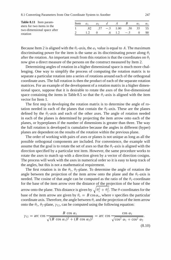
8.1 Converting Parameters from One Coordinate System to Another 247
Table 8.11 Item param-eters for two items in thetwo-dimensional space afterrotation
Item a1 a2 d A B ˛1 ˛1
1 :82 :57 �:5 1:00 :50 35 552 1:2 0 :6 1:2 �:5 0 90
Because Item 2 is aligned with the �1-axis, the a1 value is equal toA. The maximumdiscriminating power for the item is the same as its discriminating power along �1after the rotation. An important result from this rotation is that the coordinates on �1now give a direct measure of the persons on the construct measured by Item 2.
Determining angles of rotation in a higher dimensional space is much more chal-lenging. One way to simplify the process of computing the rotation matrix is toseparate a particular rotation into a series of rotations around each of the orthogonalcoordinate axes. The full rotation is then the product of each of the separate rotationmatrices. For an example of the development of a rotation matrix in a higher dimen-sional space, suppose that it is desirable to rotate the axes of the five-dimensionalspace containing the items in Table 8.5 so that the �1-axis is aligned with the itemvector for Item 1.
The first step in developing the rotation matrix is to determine the angle of ro-tation needed in each of the planes that contain the �1-axis. These are the planesdefined by the �1-axis and each of the other axes. The angle of rotation neededin each of the planes is determined by projecting the item arrow onto each of theplanes, or hyperplanes if the number of dimensions is greater than three. The waythe full rotation is developed is cumulative because the angles in different (hyper)planes are dependent on the results of the rotation within the previous plane.
The order of working with pairs of axes or planes is not unique as long as all thepossible orthogonal components are included. For convenience, the example willassume that the goal is to rotate the set of axes so that the �1-axis is aligned with thedirection specified by a particular test item. However, the same procedure works torotate the axes to match up with a direction given by a vector of direction cosigns.The process will work with the axes in numerical order so it is easy to keep track ofthe angles, but this is not a mathematical requirement.
The first rotation is in the �1, �2-plane. To determine the angle of rotation theangle between the projection of the item arrow onto the plane and the �1-axis isneeded. The cosine of that angle can be computed as the ratio of the �1-coordinatefor the base of the item arrow over the distance of the projection of the base of the
arrow onto the plane. This distance is given byq�21 C �22 . The �-coordinates for the
base of the item arrow are given by �v D B cos˛v, where v specifies the particularcoordinate axis. Therefore, the angle between �1 and the projection of the item arrowonto the �1, �2-plane, �12, can be computed using the following equation:
�12 D arc cosB cos ˛1p
.B cos ˛1/2 C .B cos ˛2/2D arc cos
cos ˛1pcos2 ˛1 C cos2 ˛2
:
(8.10)

248 8 Transforming Parameter Estimates to a Specified Coordinate System
Note that the Bs cancel in the expression. Further, because cos˛v D av
qPa2i ,
where the summation is over all of the a-parameters for the item, (8.11) gives an-other useful expression for the angle. Substituting the expression for cos˛v into(8.10), the result is
�12 D arc cos
2
66664
a1smP
iD1
a2i
sa21mP
iD1a2i
C a22mP
i�1a2i
3
77775
D arc cos
2
64
a1qa21 C a22
3
75 : (8.11)
The expression in the brackets on the right is not the expression for the cosine be-tween the item arrow and the �1-axes because the denominator does not contain allof the elements of the a-vector. It is the angle between the line projected into the �1,�2-plane and the �1-axis.
In general, the angle of rotation needed in each of the �1,�v-planes is given by
�1v D arc cos
2
66664
sv�1PiD1
cos2 ˛i
svP
iD1cos2 ˛i
3
77775
D arc cos
2
66664
sv�1PiD1
a2i
svP
iD1a2i
3
77775; for v D 2; : : : ; m:
(8.12)
Equation (8.12) results in m � 1 angles of rotation; one in each of the planes de-fined by pairing the �1-axis with each of the other axes. Note that while the formof (8.12) is the same for each coordinate axis, v, the number of terms in the sum-mations changes as the angle with each axis is computed. This indicates that theorder of applications of the rotations is important. The second angle is the amountof rotation after the first rotation has been completed. For example, if the goal isto rotate the �1-axis to coincide with the item arrow for Item 1 in Table 8.5 witha-vector [.78 .53 .24 .01 .35], then the angles of rotation computed using (8.12) are34ı, 14ı, :59ı, and 20ı and they need to be applied in that order.
The rotation matrix for the rotation in each plane is similar to (8.8). The matrixis an m � m identity matrix with four cells replaced by the following values: cell11 by cos ��1v, cell 1v by sin ��1v, cell v1 by � sin ��1v, and cell vv by cos ��1v.The negative angles are used to determine the rotation matrices because the axes arerotated to align with the item rather than rotating the item to align with the axes. Itseems more logical to consider the locations of persons and items to be fixed in thespace and the orientation of the axes to be arbitrary than to consider the items andpersons moving each time parameters are estimated.

8.1 Converting Parameters from One Coordinate System to Another 249
The four rotation matrices for this example are
2
666664
:83 �:56 0 0 0
:56 :83 0 0 0
0 0 1 0 0
0 0 0 1 0
0 0 0 0 1
3
777775;
2
666664
:97 0 �:25 0 0
0 1 0 0 0
:25 0 :97 0 0
0 0 0 1 0
0 0 0 0 1
3
777775;
2
666664
:9999 0 0 �:01 0
0 1 0 0 0
0 0 1 0 0
:01 0 0 :9999 0
0 0 0 0 1
3
777775;
and 2
666664
:94 0 0 0 �:340 1 0 0 0
0 0 1 0 0
0 0 0 1 0
:34 0 0 0 :94
3
777775:
These matrices can be applied individually in the sequence shown to perform therotation on the item parameters and the ™-vectors, or they can be multiplied togetherusing matrix multiplication to obtain a single rotation matrix,
Rot DvY
iD2Rot1i ; (8.13)
where Rot1i is the rotation matrix within the plane of �1 and �i . The order of themultiplication is important. Multiplying the rotations together in a different orderwill not give the desired result. For this example, the full rotation matrix is
2
666664
:75 �:56 �:20 �:01 �:27:51 :83 �:14 �:01 �:18:23 0 :97 �:00 �:08:01 0 0 1:00 �:00:34 0 0 0 :94
3
777775:
The item and person parameters after rotation are obtained by postmultiplyingthe a and ™ matrices by the rotation matrix, a Rot and ™Rot. The results of theapplication of the rotation to the a-matrix are given in Table 8.12 and the results forthe ™-matrix are given in Table 8.13.
Table 8.12 Discriminationparameters after rotating toalign �1-axis with the mostdiscriminating direction forItem 1
Item number a1 a2 a3 a4 a5
1 1:04 �:00 �:00 .00 �:002 :92 �:21 :17 .23 :31
3 :66 :14 :17 .03 :38
4 :68 :09 :06 .17 :49
5 :76 �:10 :19 .07 :27
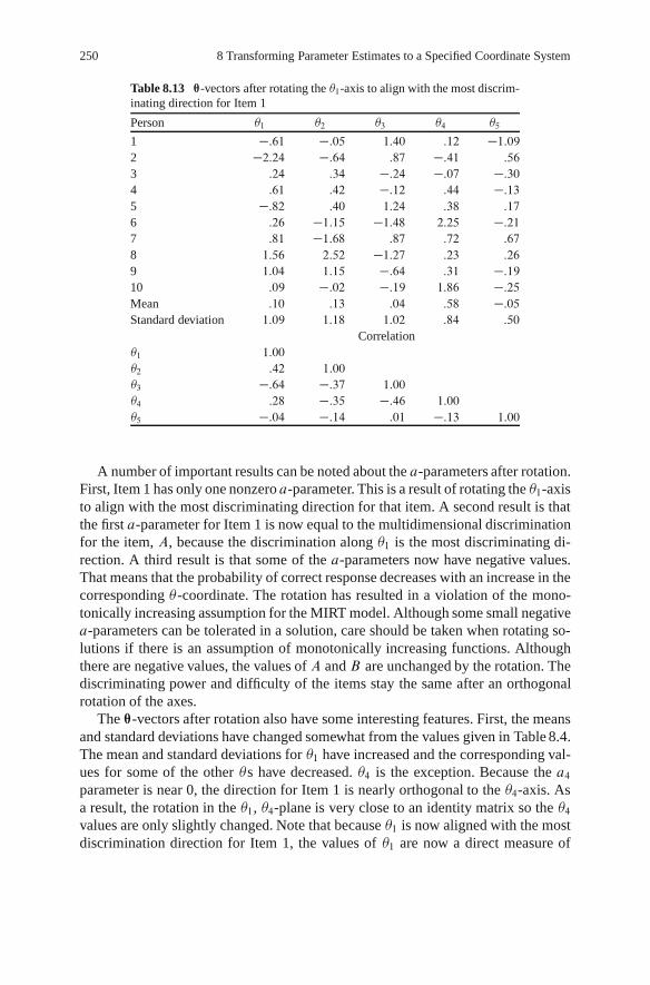
250 8 Transforming Parameter Estimates to a Specified Coordinate System
Table 8.13 ™-vectors after rotating the �1-axis to align with the most discrim-inating direction for Item 1
Person �1 �2 �3 �4 �5
1 �:61 �:05 1:40 :12 �1:092 �2:24 �:64 :87 �:41 :56
3 :24 :34 �:24 �:07 �:304 :61 :42 �:12 :44 �:135 �:82 :40 1:24 :38 :17
6 :26 �1:15 �1:48 2:25 �:217 :81 �1:68 :87 :72 :67
8 1:56 2:52 �1:27 :23 :26
9 1:04 1:15 �:64 :31 �:1910 :09 �:02 �:19 1:86 �:25Mean :10 :13 :04 :58 �:05Standard deviation 1:09 1:18 1:02 :84 :50
Correlation�1 1:00
�2 :42 1:00
�3 �:64 �:37 1:00
�4 :28 �:35 �:46 1:00
�5 �:04 �:14 :01 �:13 1:00
A number of important results can be noted about the a-parameters after rotation.First, Item 1 has only one nonzero a-parameter. This is a result of rotating the �1-axisto align with the most discriminating direction for that item. A second result is thatthe first a-parameter for Item 1 is now equal to the multidimensional discriminationfor the item, A, because the discrimination along �1 is the most discriminating di-rection. A third result is that some of the a-parameters now have negative values.That means that the probability of correct response decreases with an increase in thecorresponding �-coordinate. The rotation has resulted in a violation of the mono-tonically increasing assumption for the MIRT model. Although some small negativea-parameters can be tolerated in a solution, care should be taken when rotating so-lutions if there is an assumption of monotonically increasing functions. Althoughthere are negative values, the values of A and B are unchanged by the rotation. Thediscriminating power and difficulty of the items stay the same after an orthogonalrotation of the axes.
The ™-vectors after rotation also have some interesting features. First, the meansand standard deviations have changed somewhat from the values given in Table 8.4.The mean and standard deviations for �1 have increased and the corresponding val-ues for some of the other �s have decreased. �4 is the exception. Because the a4parameter is near 0, the direction for Item 1 is nearly orthogonal to the �4-axis. Asa result, the rotation in the �1, �4-plane is very close to an identity matrix so the �4values are only slightly changed. Note that because �1 is now aligned with the mostdiscrimination direction for Item 1, the values of �1 are now a direct measure of

8.1 Converting Parameters from One Coordinate System to Another 251
proficiency on the composite of skills and knowledge measured by that test item.These �-values are a projection onto the line defined by the direction of best mea-surement for that item.
The correlations between the �-coordinates have also changed even though anorthogonal rotation was used. For example, the correlation between �2 and �5 isnow �:14. The coordinates from the previous orientation of the axes had a corre-lation of .32. The orthogonal rotation does not maintain any of these properties ofthe �-coordinates. Although the values of both the a- and �-parameters have bothchanged, the matrix product, a™0, has not changed. The probabilities of correct re-sponse predicted by the model are unchanged when rotated parameters are used inthe model.
When MIRT calibration programs such as TESTFACT are used to obtain esti-mates of the item- and person-parameters, the orientation of the axes is fixed byconstraints and optimization procedures built into the programs. This means thatdifferent calibration programs will probably result in coordinate systems that arenot the same. Even the application of the same program to different samples ofitem response data from the same test may lead to different orientations for thecoordinate axes. Therefore, it is important to consider how to determine the rota-tion needed to place axes in the same orientation. The examples given here usedorthogonal rotations to change the orientation of the coordinate axes because thoserotations maintain the same relative location of the person locations in the ™-space.If constant distances between person locations can be assumed for two set of axes,then it is reasonable to determine the rotation between two solutions assumingorthogonality.
A useful procedure for determining the rotation is the Procrustes methodology.This methodology is named after a Greek mythological figure who purportedlywould cut off limbs that were too long, or stretch people to make them exactlyfit a bed (Bulfinch 1855, p. 124). The Procrustes methodology requires the specifi-cation of a target matrix (the bed) and then determines the rotation that minimizesthe squared distance between the rotated points and those in the target. The mathe-matical details of the Procrustes methodology are described in such texts as Gowerand Dijksterhuis (2004).
The orthogonal Procrustes rotation from one matrix to a target matrix is obtainedfrom the singular value decomposition of the matrix product of the two matrices. Ifthe target matrix is the matrix of person location coordinates, ™, and the alternatematrix is the rotated set of coordinates, �, then the singular value decomposition ofthe product is given by
svd�™0� D USV0; (8.14)
where S is a m�m diagonal matrix with positive values in the diagonal, and U andV are m �m orthogonal matrices.
The orthogonal Procrustes rotation, RP, to transform the values in � to values of™ is given by
RP D VU0: (8.15)

252 8 Transforming Parameter Estimates to a Specified Coordinate System
Because exactly the same rotation matrix was used to transform both the ™-matrixof person locations and the a-matrix of discrimination parameters, the singular valuedecomposition of the product of a target a-matrix and a rotated a-matrix can be usedto compute exactly the same rotation matrix. If the target matrix of discriminationparameters is a and the other matrix of discrimination parameters is a, then parallelequations to (8.14) and (8.15) can be specified.
svd�a0a D USV0 and RP D VU0: (8.16)
Under the conditions for the examples given here that do not include estimationerror, the rotation matrix RP will be identical when obtained from the location anddiscrimination matrices.
For the two-dimensional example given previously, the computation of the ro-tation matrix to convert the values in Tables 8.10 and 8.11 back into the values inTables 8.1 and 8.2, respectively, can be done through the following steps:
1. svd .a0a/ D svd
�:26 :97
:92 :77
�0 �:82 :57
1:2 0
�!
D svd
��1:32 :15
1:72 :55
��.
2. svd .a0a/ D USV0 D��:59 �:81
�:81 :59
� �2:22 0
0 :21
� ��:97 �:24�:24 :97
�0:
3. RP D VU0 D��:97 �:24
�:24 :97
� ��:59 �:81�:81 :59
�0D�:77 :64
�:64 :77�:
Note that the matrix RP is the inverse of the matrix given following (8.8) that wasused to perform the rotation of the axes to the new orientation. The results wouldbe exactly the same if the location coordinates for persons had been used. The sameprocess can be used for the five-dimensional example.
8.1.3 Changing the Units of the Coordinate Axes
Two sources of indeterminacy in the MIRT solutions for the compensatory modelhave been presented in the previous two sections – location of the origin of the™-space and the orientation of the coordinate axes in that space. In both cases, the as-pects of the solutions can be changed without violating the principle of invariance.The probabilities of correct response to the test items remain the same if both theitem- and person-parameters are transformed in a consistent way.
There is a third type of indeterminacy in the compensatory MIRT models. Thatindeterminacy is the unit of measurement used along each coordinate axis. Thisunit of measurement is typically set by either specifying the size of the a-parameterin a program like ConQuest, or by setting the standard deviation of the location

8.1 Converting Parameters from One Coordinate System to Another 253
coordinates to a particular value – usually 1.0 – in programs like TESTFACT. Thismeans that the results of different calibrations of the same set of item responsedata may result in different size units for the coordinate axes. For example, if thesame test were administered to two different groups of examinees, one with highvariance on �1 and the other with low variance on �1, a calibration program might setthe �1-scale for both calibrations to have a standard deviation of 1 for the estimated�1-values. The result would be that the unit of measurement on the �1-axis would belarger for the first group than the second. This change in unit would result in quitedifferent values for the item- and person-parameters estimated from the analysis ofthe two data sets. The same result can occur when different programs are used. Thedefaults for setting the units for the scales on the coordinate axes might be differentresulting in estimates that appear to be quite different.
In this section, the item- and person-parameters used in the previous sections areused to show the impact of changing the units for the coordinate axes in the formof a solution. The results are shown while keeping the origin in the same locationand the orientation of the axes the same so that the specific impact of changing unitscan be noted. In the next section, the effects of combinations of shifts in origin,rotations, and change in units are considered.
Suppose that the person location coordinates given in Table 8.1 were from a cal-ibration of a long test to a large, well selected group of examinees. The programused to estimate the parameters of the MIRT model sets the standard deviations ofthe estimated values for each dimension to 1.0, thus setting the units for the coordi-nate axes. Later the response strings for the same ten examinees shown in Table 8.1were used in a second analysis on a subsample of the first examinee sample, but thissubsample has a restricted range on �1 resulting in a standard deviation that was .8as much as the full sample, and an expansion of the range on �2 because of the in-clusion of some extreme examinees. �2 had a standard deviation that is 1.4 as largeas that for the full sample. How would the solution from the first sample compare tothat from the second sample?
Because the calibration program sets the unit for the coordinate scale as onestandard deviation, a person who had a �1-coordinate of .8 in the first analysis wouldhave a coordinate of 1.00 in the second. Because the standard deviation was smaller,the units are smaller, but the numerical value of the coordinate is bigger. This isthe same result as measuring height in feet or inches, or meters or centimeters. Ifa person is 6 ft tall, changing to the smaller inch unit results in 72 in. – a muchlarger number. In this case, all of the �1-coordinates from the first analysis wouldbe multiplied by 1=:8 D 1:25 to get the coordinate value from the second analysis.This is an example of dilation of the coordinate values.
The �2-coordinates for the second analysis show the opposite effect. Because thestandard deviation is larger, the units on the scale will be larger. A person with acoordinate of 1.4 from the first analysis would have a coordinate of 1 in the secondanalysis. The coordinates in the second analysis could be obtained from the first bymultiplying them by 1=1:4 D :714. This is an example of contraction of the scale.
Converting the coordinates using one set of units to those using another set ofunits is done by multiplying by a constant. This can be done in matrix algebra by
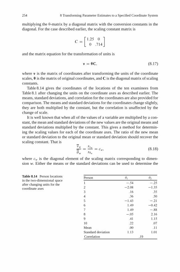
254 8 Transforming Parameter Estimates to a Specified Coordinate System
multiplying the ™-matrix by a diagonal matrix with the conversion constants in thediagonal. For the case described earlier, the scaling constant matrix is
C D�1:25 0
0 :714
�
and the matrix equation for the transformation of units is
� D ™C; (8.17)
where � is the matrix of coordinates after transforming the units of the coordinatescales, ™ is the matrix of original coordinates, and C is the diagonal matrix of scalingconstants.
Table 8.14 gives the coordinates of the locations of the ten examinees fromTable 8.1 after changing the units on the coordinate axes as described earlier. Themeans, standard deviations, and correlation for the coordinates are also provided forcomparison. The means and standard deviations for the coordinates change slightly,they are both multiplied by the constant, but the correlation is unaffected by thechange of scale.
It is well known that when all of the values of a variable are multiplied by a con-stant, the mean and standard deviations of the new values are the original means andstandard deviations multiplied by the constant. This gives a method for determin-ing the scaling values for each of the coordinate axes. The ratio of the new meanor standard deviation to the original mean or standard deviation should recover thescaling constant. That is
�w
�w
D s�w
s�w
D cw; (8.18)
where cw is the diagonal element of the scaling matrix corresponding to dimen-sion w. Either the means or the standard deviations can be used to determine the
Table 8.14 Person locationsin the two-dimensional spaceafter changing units for thecoordinate axes
Person �1 �2
1 �:54 �:252 �2:08 �1:353 :16 :35
4 :36 :50
5 �1:43 �:216 1:49 �0:427 1:49 �:888 �:05 2:16
9 :41 1:15
10 :22 :07
Mean :00 :11
Standard deviation 1:13 1:01
Correlation .19

8.1 Converting Parameters from One Coordinate System to Another 255
scaling constants, but sometimes it is more useful to use one of the statistics thanthe other. For example, if the coordinate values have originally been scaled to havea mean of 0, then multiplying that mean by a constant results in a 0 for the mean ofthe coordinates with the new units. The ratio 0/0 is not defined. In that case, usingthe standard deviations to determine the scaling constants will be more useful.
Determining the scaling constants using the values of the means and standarddeviations from Tables 8.1 and 8.14 identify an important problem with the levelof accuracy used to report the statistics. The values in the tables are rounded totwo decimal places. If they are used to determine the scaling constants, values of.6875 and 1.255 might be obtained instead of .7143 and 1.25, respectively. Thesedifferences are due solely to rounding error. If the means and standard deviationswere computed to more decimal places (e.g., 15), the scaling constants would berecovered with high precision.
To maintain the invariance property of the MIRT model, the item parametersmust be converted after the change in unit for the coordinate axes. To determinethe appropriate conversion for the item parameters, the linear exponent of the com-pensatory MIRT model is considered. The numerical value of that exponent mustremain the same after the change in scale for the probability of response from themodel to remain the same. In the case of change in units on the coordinate scales,the new scale values are given by �jw D cw�jw, were j is the index for person and wis the index for dimension. Then, �jw D �jw=cw. This expression can be substitutedfor the �-variables in the expression for the exponent of the model. In the simpletwo-dimensional case, this yields
a1�1 C a2�2 C d D a1�1
c1C a2
�2
c2C d D a1
c1�1 C a2
c2�2 C d: (8.19)
In this expression, the person index, j , is not included to simplify the notation.Equation (8.19) shows that, to maintain the same value of the exponent, the dis-crimination parameters, aw, are divided by the corresponding scaling constant. Thed -parameter is not changed. In matrix algebra terms, the a-parameters in the ™-spacewith the new units for the coordinate axes can be obtained by multiplying the origi-nal a-parameters by the inverse of the matrix of the scaling constants, aC�1.
The item parameters for the coordinate space with the new units on the coordi-nate axes are given in Table 8.15 along with the other descriptive statistics for thetest items. Note that the multidimensional discrimination, A, the multidimensionaldifficulty,B , and the angles with the coordinate axes are all different than the valuesin Table 8.2. This is a very important observation because it implies that changes in
Table 8.15 Item parameters for two items in the two-dimensionalspace after a change in units on the coordinate axes
Item a1 a2 d A B ˛1 ˛1
1 .21 1.35 �:5 1.37 .37 81 92 .74 1.08 .6 1.31 �:46 56 34

256 8 Transforming Parameter Estimates to a Specified Coordinate System
the units on the scales of the coordinate axes are the equivalent of a nonorthogonalrotation of the axes. The original and new ™-locations and item vectors are shown inFig. 8.6 to help clarify this point.
The scaling constants can be estimated from the original and converted sets ofa-parameters just as they were from the two-sets of ™-coordinates. In theory, thescaling constants can be computed from the two sets of parameters for one item, butfor estimated item parameters, the estimates of the scaling constants will be morestable based on the means of the a-parameters,
cw D Naow
Nanw; (8.20)
where cw is the scaling constant for coordinate axis w, aow is the original set ofa-parameters for dimension w, and anw is the set of a-parameters for dimension wafter change of scale.
A number of the results of the change of scale for the coordinate axes can beobserved in Fig. 8.6. First, the person locations are further from the origin on thehorizontal scale. That is, the variance of the �1-coordinates is larger as a resultof the transformation. This is the dilation of the locations because of the use of asmaller unit on the �1-axis. Correspondingly, the locations are shifted toward theorigin on the vertical scale. The variance of the �2-coordinates is smaller as a resultof the transformation. This is the contraction of the locations because of the use oflarger units on the �2-axis.
–3 –2 –1 0 1 2 3–2
–1.5
–1
–0.5
0
0.5
1
1.5
2
2.5
3
3.5
θ1
θ 2
Fig. 8.6 Person locations and item arrows before and after change of scale of coordinate axes(initial locations – circles; new locations – dots: initial item arrows – dashed lines; new item arrows– solid lines)

8.1 Converting Parameters from One Coordinate System to Another 257
A second result is the shift of the item arrows. The item arrow for Item 1 hasshifted to be closer to the �2-axis and its length has increased indicating a higherlevel of discrimination in the direction of best measurement. The increased lengthreflects the increase in value ofA after the change in units. Because this item is moresensitive to changes along �2 than �1, the use of larger units along �2 means that thetest item is sensitive to smaller changes in numerical values of location along thataxis. This is represented by an increase in the maximum slope for the surface for thattest item. Item 1 has a slight decrease in maximum slope for the opposite reason, theuse of smaller units for the �1-axis. Of course, the locations of the persons and thecharacteristics of the items have not changed. The change in the descriptive statisticsfor the test items is solely the result of the change in units for the coordinate axes.
The change in units for the coordinate axes is accomplished in exactly the sameway for the five-dimensional case. The constants for converting from the originalset of units to the new set of units are placed in the cells of a diagonal matrix thatcorrespond to the appropriate axis. New vectors of ™-coordinates are obtained bypostmultiplying the ™-matrix by the diagonal scaling matrix, C. The a-parametermatrix is postmultiplied by the inverse of the C-matrix.
8.1.4 Converting Parameters Using Translation, Rotation,and Change of Units
The previous three sections have discussed the three types of indeterminacy thatare present in the linear compensatory MIRT models. Each was considered as aseparate type of change to a coordinate system while keeping the other two typesunchanged. This section considers changes to the coordinate system that use allthree kinds of transformations – shift in origin, rotation of axes, and change in unitson the coordinate axes. In all cases, however, four important assumptions are made.
1. The relative locations of the persons in the space defined by the MIRT modelare unchanged. The only thing that is changing is the coordinate system used todescribe the locations of the persons.
2. The capabilities of the test items for distinguishing among person locations re-main unchanged. The statistical descriptions of the items may change because ofchanges in the coordinate system, but these are only different ways of describingthe same characteristics.
3. As a result of 1. and 2., the predicted probability of the observed response foreach person to each test item remains unchanged. This is the invariance propertyof the MIRT model.
4. The coordinate axes in all cases are orthogonal to each other. Only orthogonalrotations have been used to change coordinate systems.
When deciding to change the coordinate system for a solution, a decision mustbe made on the order that the various conversions are used. If a change in the unitsfor the coordinate axes is made first, then a shift in the origin is made in the new

258 8 Transforming Parameter Estimates to a Specified Coordinate System
units. Making the same numerical shift in the coordinates of the origin first usesthe original units for the coordinate axes and a subsequent change in units, evenusing the same multiplicative constants, will give a different result for coordinatesof points in the ™-space. Rotations of the coordinate axes are always made usingthe origin of the ™-space as the center of rotation. As a result, a rotation performedbefore a shift in the origin will result in a different solution than a rotation after ashift in the origin. If there are fixed matrices for rotation of a solution and scalingthe units of the coordinate axes and a fixed vector of distances for a shift in theorigin of the space, there are six possible expressions for transforming the ™-space.Each of the expressions yields a different set of numerical values for the coordinatesrepresenting the location of the same person. Although there are six representationsfor that location, the location itself has not changed – only the orientation of thecoordinate axes and the units on the axes have changes.
The expressions for the six possible transformations are given in (8.21a) through(8.21f) with � representing the matrix of coordinates in the transformed system and™ representing the matrix of original coordinates. The Rot and C matrices and the•-vector have the same definitions as was used when describing the shift in thecoordinate axes. The “1” in the expression is a n � 1 vector of 1s used to produce amatrix with identical rows of shift values for the origin of the coordinate system.
� D .™ � 1•/RotC; (8.21a)
� D .™ � 1•/C Rot; (8.21b)
� D .™Rot � 1•/C; (8.21c)
� D .™C � 1•/Rot; (8.21d)
� D ™Rot C � 1•; (8.21e)
� D ™C Rot � 1•: (8.21f)
To show the effect of each of these transformations, they have been applied tothe ™-matrix given in Table 8.1. The translation, rotation, and scaling transforma-tions are the same as were used in the two-dimensional examples in this chapter.The coordinates for each of the transformations along with the means, standard de-viations, and correlations of the coordinates are given in Table 8.16.
There are a number of important results shown in Table 8.16. First, none of thetransformed coordinates have the same means and standard deviations. Second, eachof the six transformations yields a different set of �-coordinates. Each of the trans-formations gives a uniquely different result. A third important result is the differencein correlations for the different transformations. The original correlation was .19.After the transformations, the correlations are either .44 or �:08. It is clear thatquite different correlations can result from different transformations of the coordi-nate system.
However, there are similarities among various coordinate sets that highlight someof the features of the transformations. Transformations (a), (c), and (e) have the

8.1 Converting Parameters from One Coordinate System to Another 259
Tab
le8.
16C
oord
inat
esbe
fore
and
afte
rsi
xdi
ffer
ent
tran
sfor
mat
ions
in(8
.21)
Pers
onO
rigi
nal
8.21
a8.
21b
8.21
c8.
21d
8.21
e8.
21f
1�:43
�:36
�1:81
1:47
�2:03
2:31
�3:20
:72
�1:47
2:20
�2:70
1:00
�2:58
1:15
2�1:67
�1:89
�4:23
1:19
�3:92
2:46
�5:62
:44
�3:35
2:35
�5:12
:73
�4:46
1:30
3:13
:49
�:60
1:68
�1:11
2:32
�1:99
:93
�:54
2:22
�1:49
1:21
�1:65
1:17
4:29
:70
�:27
1:72
�:86
2:31
�1:66
:97
�:29
2:20
�1:16
1:25
�1:40
1:15
5�1:15
�:29
�2:45
1:83
�2:69
2:91
�3:83
1:08
�2:12
2:81
�3:33
1:37
�3:23
1:76
61:19
�:59
�:44
0:60
�:59
:88
�1:83
�:15
�:02
0:77
�1:33
:13
�1:13
�:28
71:19
�1:23
�:96
0:25
�:88
:53
�2:35
�:50
�:31
0:42
�1:85
�:22
�1:42
�:63
8�:04
3:02
1:28
3:13
�:11
3:84
�:11
2:38
:46
3:73
:39
2:67
�:65
2:68
9:33
1:61
:49
2:20
�:40
2:77
�:89
1:44
:16
2:67
�:39
1:73
�:95
1:62
10:17
:10
�:87
1:44
�1:24
2:07
�2:26
:69
�:68
1:96
�1:76
:97
�1:79
:91
Mea
n:00
:16
�:98
1:55
�1:38
2:24
�2:37
:80
�:82
2:14
�1:87
1:08
�1:93
1:08
Stan
dard
devi
atio
n:90
1:41
1:55
:80
1:17
:95
1:55
:80
1:17
:95
1:55
:80
1:17
:95
Cor
rela
tion
.19
.44
�:08
.44
�:08
.44
�:08

260 8 Transforming Parameter Estimates to a Specified Coordinate System
same value for the correlations as do transformations (b), (d), and (f). The first threetransformations use RotC as the multiplier of ™ while the second set use CRot.Within those same sets of transformations the standard deviations of the coordi-nates are the same as well, while different across the two sets. The reason for thedifferent results is that the rotations are applied to results on different scales. TheRotC transformation performs the rotation on the original ™ coordinates and thentransforms the units for the coordinate axes of the results, while CRot transformsthe units of the coordinate axes first and then does the rotation on the transformedcoordinates. The different transformations of units of the coordinate axes cause thedifferences in the standard deviations and correlations.
To maintain the invariance properties of the MIRT model, each of these trans-formations of ™-coordinates must also be accompanied by a transformation of itemparameters. One way to determine the transformation of the item parameters is tosolve each of the equations in (8.21a) to (8.21f) for ™ and then substitute the resultinto the general expression in the exponent of the MIRT model, a™0 C d1 After thesubstitution, the multiplier of � is the transformed matrix of a-parameters and thesummative term contains the transformed d-parameters. The equations in (8.22a) to(8.22f) are the exponents after the substitution for each of the equations in (8.21a)to (8.21f). Brackets have been placed around the terms that are the converted a- andd-parameters. The expressions are in pairs with the main difference in each pair be-ing a reversal in the order of the product of R and C. The other difference in theexpressions is the multiplier of a in the intercept term. That multiplier is dependenton whether the shift in the origin of the space occurs before, (8.22a) and (8.22b), orafter a rotation or change in unit. To be consistent with the expressions in (8.21), the1 is a n � 1 vector of 1s so the transpose is a 1 � n vector of 1s.
ha.RotC/�10
i�0 C
ha•
0 C di
10
; (8.22a)
ha.CRot/�10
i�0 C
ha•
0 C di
10
; (8.22b)
ha.RotC/�10
i�0 C
ha.•Rot�1/0 C d
i10; (8.22c)
ha.CRot/�10
i�0 C
ha.•C�1/0 C d
i1
0
; (8.22d)
ha.RotC/�10
i�0 C
ha.•.RotC/�1/0 C d
i1
0
; (8.22e)
ha.CRot/�10
i�0 C
ha.•.CRot/�1/0 C d
i1
0
: (8.22f)
Table 8.17 shows the original item parameters and descriptive statistics for theitems from the two-dimensional item set and the transformed item parameters cor-responding to each of (8.22a) to (8.22f). The transformations of the item parametershave a similar pattern to the transformation of the ™-vectors. The d-parameters are

8.2 Recovering Transformations from Item- and Person-Parameters 261
Table 8.17 Initial and transformed item parameters for items in the two-dimensional space
Item a1 a2 d A B ˛1 ˛1
1 :26 :97 �:5 1 :5 75 152 :92 :77 :6 1:2 �:5 40 508.22a :66 :80 �:95 1:04 :91 51 39
:96 0 1:67 :96 �1:74 0 908.22b 1:03 :90 �:95 1:37 :69 41 49
1:26 :35 1:67 1:31 �1:28 16 748.22c :66 :80 :56 1:04 �:54 51 39
:96 0 3:00 :96 �3:12 0 908.22d 1:03 :90 �1:44 1:37 1:05 41 49
1:26 :35 :99 1:31 �:76 16 748.22e :66 :80 :01 1:04 �:01 51 39
:96 0 2:52 :96 �2:63 0 908.22f 1:03 :90 :65 1:37 �:48 41 49
1:26 :35 2:76 1:31 �2:11 16 74
different in every case. There are only two different sets of a-parameters. Thesedepend on the order of the product of R and C. The values of A and ’ follow thepattern of the a-parameters and B follows the pattern of the d-parameters.
8.2 Recovering Transformations fromItem- and Person-Parameters
There are many situations when it is desirable to convert from one coordinatesystem to another, but the form of transformation from one set of person- or item-parameters is unknown. Perhaps the most important case when determining the formof the transformation needed is in linking of multiple calibrations to get the valuesof the parameter estimates in the same ™-space, or for the equating of test forms.These cases will be discussed in detail in Chap. 9. Other cases are when the recov-ery of parameters using various calibration programs is being investigated, or whenthe solutions from different calibrations programs are being compared. These areasof research require that the item- and person-parameter estimates be placed in thesame ™-space before they can be compared.
Two cases will be considered in this section. The first is when two sets of™-vectors are available for the same people. This case holds when two programs thatestimate the ™-vectors are applied to the same item-score matrix, or when there are™s used to generate data and ™-estimates are available from a program. The secondcase is when two sets of item-parameters are available for the same test items. Thisoccurs when there are common items in two test forms that are separately calibratedor when an item parameter recovery study is performed.

262 8 Transforming Parameter Estimates to a Specified Coordinate System
8.2.1 Recovering Transformations from �-vectors
Suppose that a group of individuals have been administered a very long andhigh quality test that allows the accurate estimation of their locations in a five-dimensional proficiency space. Because the test is long and of high quality, and thecalibration program is very good, the estimates of ™-vectors are assumed to have solittle error that the amount of error can be ignored. The ™-vectors are treated as errorfree estimates of location. However, the group of individuals has been included intwo separate convenience samples that are used for calibration. Therefore, becauseof the way that the calibration program deals with the indeterminacy in the model,the location of the origin, orientation of the axes, and units of measurement mightnot be the same. The question of interest is whether the ™-vectors obtained from thetwo calibrations represent the same locations in the ™-space.
The first ten of the ™-vectors from the first calibration are given in Table 8.18along with the means, standard deviations, and correlations for the coordinate esti-mates for each axis. The descriptive statistics are for this sample of ten observations.Because of the small sample, the correlations are not significantly different than 0 atthe .05 level. This set of ™-vectors is arbitrarily selected as the base set and is labeled™b. The goal will be to determine if the second set of ™-vectors can be transformedto be the same as the base set.
The second set of ™-vectors and their descriptive statistics are given in Table 8.19.This alternate set of ™-vectors is represented as the matrix ™a. The descriptive
Table 8.18 ™-vectors for the Base Set
Person �b1 �b2 �b3 �b4 �b5
1 �:43 �:36 1:30 :12 �1:242 �1:67 �1:89 :27 �:43 �:223 :13 :49 �:16 �:07 �:214 :29 :70 :03 :44 :08
5 �1:15 �:29 :99 :37 �:116 1:19 �:59 �1:36 2:25 �:117 1:19 �1:23 :98 :72 :90
8 �:04 3:02 �:89 :24 :76
9 :33 1:61 �:36 :32 :16
10 :17 :10 �:14 1:86 �:20Means :00 :16 :07 :58 �:02Standard deviations :90 1:41 :85 :84 :59
Correlations�b1 1:00
�b2 :19 1:00
�b3 �:40 �:47 1:00
�b4 :63 �:07 �:45 1:00
�b5 :41 :32 �:31 :07 1:00
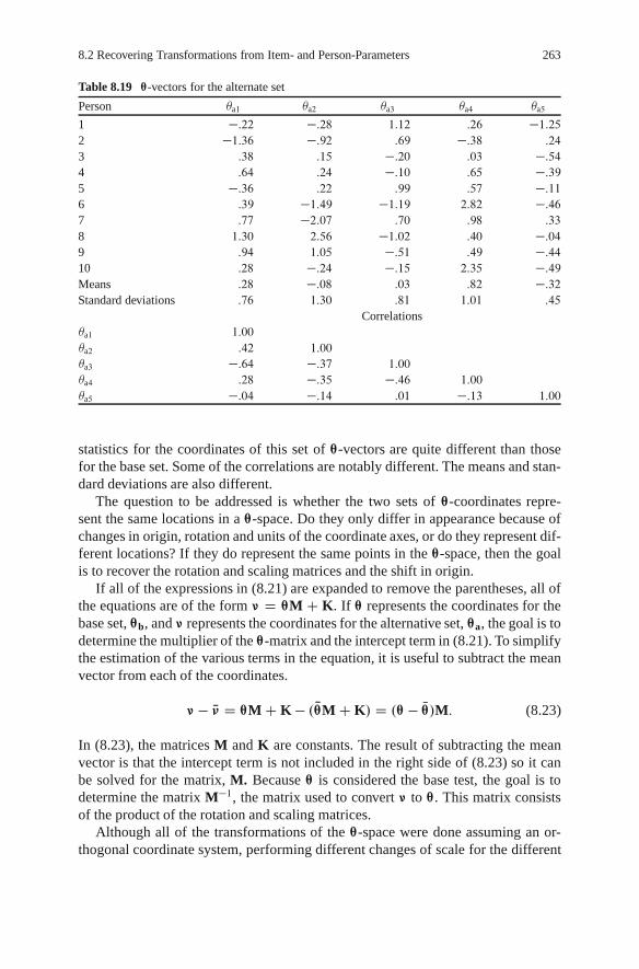
8.2 Recovering Transformations from Item- and Person-Parameters 263
Table 8.19 ™-vectors for the alternate set
Person �a1 �a2 �a3 �a4 �a5
1 �:22 �:28 1:12 :26 �1:252 �1:36 �:92 :69 �:38 :24
3 :38 :15 �:20 :03 �:544 :64 :24 �:10 :65 �:395 �:36 :22 :99 :57 �:116 :39 �1:49 �1:19 2:82 �:467 :77 �2:07 :70 :98 :33
8 1:30 2:56 �1:02 :40 �:049 :94 1:05 �:51 :49 �:4410 :28 �:24 �:15 2:35 �:49Means :28 �:08 :03 :82 �:32Standard deviations :76 1:30 :81 1:01 :45
Correlations�a1 1:00
�a2 :42 1:00
�a3 �:64 �:37 1:00
�a4 :28 �:35 �:46 1:00
�a5 �:04 �:14 :01 �:13 1:00
statistics for the coordinates of this set of ™-vectors are quite different than thosefor the base set. Some of the correlations are notably different. The means and stan-dard deviations are also different.
The question to be addressed is whether the two sets of ™-coordinates repre-sent the same locations in a ™-space. Do they only differ in appearance because ofchanges in origin, rotation and units of the coordinate axes, or do they represent dif-ferent locations? If they do represent the same points in the ™-space, then the goalis to recover the rotation and scaling matrices and the shift in origin.
If all of the expressions in (8.21) are expanded to remove the parentheses, all ofthe equations are of the form � D ™M C K. If ™ represents the coordinates for thebase set, ™b, and � represents the coordinates for the alternative set, ™a, the goal is todetermine the multiplier of the ™-matrix and the intercept term in (8.21). To simplifythe estimation of the various terms in the equation, it is useful to subtract the meanvector from each of the coordinates.
� � N� D ™M C K � . N™M C K/ D .™ � N™/M: (8.23)
In (8.23), the matrices M and K are constants. The result of subtracting the meanvector is that the intercept term is not included in the right side of (8.23) so it canbe solved for the matrix, M. Because ™ is considered the base test, the goal is todetermine the matrix M�1, the matrix used to convert � to ™. This matrix consistsof the product of the rotation and scaling matrices.
Although all of the transformations of the ™-space were done assuming an or-thogonal coordinate system, performing different changes of scale for the different

264 8 Transforming Parameter Estimates to a Specified Coordinate System
coordinate axes can result in a change in the angles between item vectors and achange in the correlation between coordinate axes. As a result, the rotation from� to ™ is determined using the nonorthogonal Procrustes solution (e.g., Gower andDijksterhuis 2004). In this case, the rotation is given by
M�1 D �.� � �/0 .� � �/
�1.� � �/0
�™ � ™
: (8.24)
The matrix M�1 is the product of the rotation matrix Rot�1 and the scaling matrixC�1 and the order of the product is important because matrix multiplication does nothave the commutative property, AB ¤ BA. A different M�1 results from the twopossible orders for the product. For the coordinates presented in Tables 8.18 and8.19, the matrix M�1 is given by
2
666664
1:08 :73 :34 :01 :48
�:51 :75 :00 :00 �:00�:26 �:17 1:21 :00 :00
�:01 �:00 �:00 :83 �:00�:30 �:20 �:09 �:00 1:05
3
777775:
When this matrix is postmultiplied times the matrix of deviations from the coor-dinate means for the alternate coordinate values, � D ™a, the result is exactly thevalues of the deviations from the coordinate means for the base coordinate values,™b. The inverse of this matrix can be used as part of the transformation from ™b to™a. The inverse of matrix, M�1,
�M�1�1 D M is
2
666664
:53 �:62 �:17 �:01 �:24:36 :91 �:11 �:01 �:16:16 :00 :77 �:00 �:07:01 �:00 �:00 1:2 �:00:23 �:00 :00 �:00 :85
3
777775:
The matrix M can also be determined directly by determining the nonorthogonalProcrustes rotation for transforming ™ to �. This transformation is obtained by sub-stituting ™ for � and � for ™ in (8.24).
According to the way that the transformation of the base coordinate system to thealternate coordinate system was conducted, it is known that M is the product of anorthogonal rotation matrix and a diagonal matrix of positive values for convertingthe units on the coordinate axes. A singular value decomposition (e.g., Gentile 1998)factors matrices into component parts that have these properties so it can be used torecover Rot and C. The result of a singular value decomposition is a set of threematrices – U, †, and V – where U and V are orthogonal matrices and † is a diag-onal matrix with positive values such that M D U†V0. The decomposition of theM-matrix given earlier yields

8.2 Recovering Transformations from Item- and Person-Parameters 265
U D
2
666664
:01 �:56 �:27 :21 �:76:00 :83 �:18 :14 �:51:00 :00 �:08 �:97 �:23�1 0 �:00 �:00 �:01:00 :00 :94 �:00 �:33
3
777775;† D
2
666664
1:2 0 0 0 0
0 1:1 0 0 0
0 0 :9 0 0
0 0 0 :8 0
0 0 0 0 :7
3
777775; and
V D
2
666664
0 0 0 0 �1:00 1 �:00 :00 0
:00 :00 �:00 �1 0
�1 0 �:00 :00 0
�:00 :00 1 :00 0
3
777775:
These matrices have interesting properties. Either one of the U or V matricesmight be composed of 0s and C1 s or �1 s. In this case it is matrix V. The matrixwith this form has the function of rearranging the rows, columns, and signs of valuesin the transformation matrix so that the coordinates match on direction of increasingvalues and the appropriate axes match each other. The †-matrix contains the scalingfactors used to change the units on the axes, but for the MATLAB (2007) solutionreported here, these have been ordered from large to small. That order is not nec-essarily the order in the original scaling of the axes. The original ordering can bedetermined multiplying the absolute value of the rearrangement matrix, in this caseV, times a column vector with the diagonal values of †. In this case, the result is theordering of scaling factors of [.7 1.1 .8 1.2 .9]0. Thus, the original scaling matrix, C,is a matrix with these values in the diagonal.
The original rotation matrix, Rot, can be obtained by UV0. The matrix that isthe rearrangement matrix indicates the order of the initial product of Rot and Cproviding the initial transformation from ™ to �. If V is the rearrangement matrix,the order was RotC. If U is the rearrangement matrix, the order is CRot. For theexample given here the recovered matrix
Rot D
2
666664
:75 �:56 �:21 �:01 �:27:51 :83 �:14 �:00 �:18:23 �:00 :97 �:00 �:08:01 �:00 �:00 1:00 �:00:33 �:00 �:00 �:00 :94
3
777775:
This is the matrix used to rotate the �1-axe to align with the direction of greatestdiscrimination for the first item in the example item set.
The transformation from the alternate set of coordinates to the base set of co-ordinates requires another term to account for the shift in origin, K. Solving thegeneral equation for the conversion from one set of coordinates to another for K,� D ™M C K, for K yields K D � � ™M. But, the rows of K are constant since theshift in origin is the same for all ™-points. Therefore, the means of the columns of

266 8 Transforming Parameter Estimates to a Specified Coordinate System
K give the same shift in origin as the individual rows. Thus, a vector of translationof origin values can be obtained from
K D � � ™M: (8.25)
Solving � D ™M C K, for ™ and substituting for K yields
™ D �M�1 � KM�1 D �M�1 � 10 �� � ™M
M�1 D �M�1 C 10 �™ � �M�1 :(8.26)
where 10 is a 1 x n vector of 1s. The last term on the right gives the term that accountsfor the shift in origin. This term is given the variable name, k, resulting in the finalexpression for the conversion of the alternate set of coordinates to the base set as
™ D �M�1 C 10k: (8.27)
For the example, k D Œ�:42 � :04 � :10 � :10 :18. This is not the set of transla-tion values for the initial transformation of the ™-coordinates. The transformationused to produce the alternate ™-coordinates for this example was that given in(8.21c). If that equation is solved for ™ in terms of �, the k term in (8.27) is found tobe equal to •Rot�1. Therefore, multiplying k by Rot will recover the original vectorof values used to translate the origin Œ�:3 :20 � :1 :3. However, there is no way todetermine the terms that are multiplied together to form the k-term in the equation.That term might be •, or • multiplied by the inverse of Rot or C or both.
8.2.2 Recovering Transformations Using Item Parameters
The perspective taken in this chapter has been that the space of interest in MIRTanalysis is the space defined by the location of persons. These locations are indicatedby vectors of ™-coordinates. The origin of the space, the rotation of the axes, and theunits used on the coordinate axes are arbitrary decisions of the person performingthe analysis, or the person writing the estimation program used to obtain estimates ofthe model parameters. Previous sections of this chapter have shown how the ™-spacecan be transformed and how the item parameters need to be transformed to main-tain the invariance property of the MIRT model. The last section showed how therelationship between representations of the same ™-space can be determined usingthe original and alternate sets of ™-coordinates. In many applications of MIRT, twosets of coordinate representations are not available for the same persons. However,item parameter estimates may be available for the same items in the two coordinatesystems. This section shows how to determine the relationship between two coor-dinate systems that represent the same ™-space using item parameters that result ininvariant probabilities of response from the two coordinate systems.

8.2 Recovering Transformations from Item- and Person-Parameters 267
8.2.2.1 Recovery of the Rotation and Scaling Matrices
The transformation of the �-coordinates shown in (8.22a) is used here to providean example of the logic behind the recovery of the rotation matrix, Rot, and thescaling matrix, C. It is assumed that the item parameters for the multidimensionalextension of the two-parameter logistic model were transformed to be consistentwith the transformation of the �-coordinates so that the invariance property of theMIRT model holds. This means that the expressions for the exponents of the modelfor the same person and items should yield identical values. That is,
¤�0 C —1 D a™0 C d1; (8.28)
where ¤ is the matrix of discrimination parameters for the transformed space, � isthe matrix or person parameters after transformation, and — is the intercept parame-ter after transformation. The other parameters are as defined previously.
The relationship between the item parameters before transformation to those aftertransformation can be determined by substituting the expression for the transforma-tion of ™ to obtain � in place of � in (8.28). The result is given in (8.29).
¤�™RotC � 1•0RotC
0 C —1 D ¤ .™RotC/0 � �1•0RotC
0 C —1
D ¤C0Rot0™0 � �1•0RotC
0 C —1: (8.29)
Comparison of the second line of (8.29) with the right side of (8.28) shows that themultiplier of ™0 in (8.29) is the equivalent of a in (8.28).
a D ¤C0Rot0: (8.30)
Because a and ¤ are known, the equation in (8.30) can be solved for C0Rot0. Inthis case, the same nonorthogonal Procrustes procedure is used as was used to de-termine the rotation and scaling of the ™-coordinates. That is, the a-matrix is usedas the target matrix and the nonorthogonal Procrustes rotation is used to determinethe transformation from ¤ to a.
To demonstrate the recovery of the rotation matrix and the scaling matrix, thea-parameters given in Table 8.5 were transformed to be consistent with the trans-formation of the coordinate system in (8.21a). The transformed discriminationparameters are given in Table 8.20. The original parameters in Table 8.5 are usedas the target for the Procrustes rotation procedure and the transformation matrixwas determined for rotating and scaling the parameters in Table 8.20 to match theoriginal set. That is,
C0Rot0 D �¤0¤
�1¤0a: (8.31)

268 8 Transforming Parameter Estimates to a Specified Coordinate System
Table 8.20 Discriminationparameters after rotating toalign �1-axis with the mostdiscriminating direction forItem 1 and changing the unitson the coordinate axes
Item number �1 �2 �3 �4 �5
1 1:48 :00 �:00 .00 �:002 1:32 �:19 :22 .19 :34
3 :94 :13 :21 .02 :42
4 :98 :08 :07 .14 :55
5 1:08 �:09 :24 .06 :30
For the item parameters in the example, the result is
C0Rot0 D
2
666664
:53 :36 :16 :01 :23
�:62 :91 �:00 �:00 �:00�:17 �:11 :77 :00 �:00�:01 �:01 �:00 1:20 �:00�:24 �:16 �:07 �:00 :85
3
777775:
Note that this matrix is the transpose of the matrix, M, used to transform thecoordinate axes (see (8.23)). It can be decomposed into the rotation and scalingmatrices using the singular value decomposition in the same way that was done forM. Postmultiplying � by the matrix given earlier will exactly recover the originala-parameters because in this case all of the values are true parameters without esti-mation error.
8.2.2.2 Recovery of the Translation of Origin
The recovery of the translation of the origin of the ™-space from the differencesin the item parameters is surprisingly difficult. The reason for the difficulty is thatthe item parameters do not give information about whether the translation of originoccurred on the original ™-space before rotation and scaling, or after one or both ofthe rotation and scaling transformations. It is possible to determine the multiplierof the a-matrix in the right hand terms of (8.22a) to (8.22f). In some cases, thismultiplier is the •-vector of values used to translate the origin of the ™-space, butin other cases, the •-vector is multiplied by functions of the rotation and scalingmatrices.
The terms on the right side of (8.22a) to (8.22f) are the possible definitions of theintercept term of the model after transformation of the ™-space. These transformedintercept terms maintain the invariance property of the model. In every case theyare in the form of the a-matrix multiplied times a term plus d. The general symbolused for the multiplier of a is �. Using this notation, the transformed value of theintercept term is given by
Qd D a� C d: (8.32)
The solution for d is simplyQd � a� D d; (8.33)

8.3 Transforming the ™-space for the Partially Compensatory Model 269
but the value of � is needed to transform the intercept parameter from the alternate�-space back to the initial ™-space. Solving for � is complicated slightly by thefact that a is typically not a square matrix so the equation cannot be solved withthe simple inverse of a. However, with a little matrix manipulation, the followingequation can be used to solve for �.
� D �a0a�1
a0 � Qd–d: (8.34)
The matrix that is the result of (8.34) can substituted into (8.33) to recover d from Qd.This may seem like a tautology because (8.34) requires the knowledge of d. How-ever, this equation is often used when � is determined from a subset of all of theitems that have the intercept terms from both representations of the ™-space and thenit can be applied to the items that are not contained in that subset. This applicationof the procedure will be described in more detail in Chap. 9. The same result that isshown here was derived in a different way by Joseph Martineau and that derivationis present in Reckase and Martineau (2004).
It seems that it should be possible to determine the translation of origin of theperson space from the item parameters that yield invariant probabilities. At thispoint in time, the procedure for doing this has not been determined. It is left tothe next generation of psychometricians to work out the finer details about how torecover the translation of origin from the two sets of item parameters.
The relationships presented in this part of the chapter have been developed as-suming the multidimensional generalization of the two-parameter logistic model.They generalize directly to the multidimensional normal ogive model and to otherlogistic models including those for polytomous items. The same relationships alsohold for the multidimensional generalization of the three-parameter logistic modelwhen there is a single c-parameter for each item. That is, there is a single lowerasymptote for the item response surface. It is left to the reader to confirm thegeneralizations.
8.3 Transforming the ™-space for the PartiallyCompensatory Model
The transformation of the proficiency space has quite different effects on the itemparameters for the partially compensatory model than it does on the item parametersfor the compensatory model. Although it is possible to consider the same transfor-mations to the ™-space as those given in Sect. 8.1, the rotation of axes is not allowedby the model. Because the equiprobable contours for the partially compensatorymodel have asymptotes that are parallel to the coordinate axes, rotating the axes,but keeping the location of the item response surface constant would result in amodel that is mathematically unwieldy. Estimation of the item parameters for this

270 8 Transforming Parameter Estimates to a Specified Coordinate System
model fixes the orientation of the coordinate axes. There is still indeterminacy in themodel concerning the origin of the space and the units on the coordinate axes.
The partially compensatory model that was presented in (4.18) is repeated herefor convenience:
P.Uij D 1j™j ; ai ;bi ; ci / D ci C .1 � ci /
mY
`D1
e1:7ai`.�j`�bi`/
1C e1:7ai`.�j`�bi`/
!
: (8.35)
Suppose that the original ™-space is transformed to have a different origin as wasdone in (8.1). That is, the new coordinates for the locations of persons are deter-mined by subtracting shift constants from the coordinates on each axis. The amountof shift need not be the same – � D � � ı. To maintain the invariance property ofthe MIRT model, it is only necessary to add the same shift constant to the difficultyparameters for each dimension. That is, the difficulty parameters in the new personspace are b � •. Substituting the two sets of translated values into (8.35) results inexactly the same probabilities of responses as the original set of parameters.
Similarly, if the units of the coordinate axes are changed by multiplying eachby a constant and the constants are collected into the diagonal of a diagonal matrixC, the coordinates of the locations of persons are multiplied by this matrix, thatis ™C. Then the invariance property of the MIRT model is maintained if the samescaling is performed on b, bC, and the inverse scaling is performed on a, aC�1.These transformations are conceptually the same as those that result in invarianceof probabilities for the unidimensional IRT models.
If coordinates for the same persons are available from the original person spaceand the transformed one, the details of the transformations can be determined inthe same way as described in Sect. 8.2. If the item parameters are available for thesame items as represented in two different coordinate systems, the functions usedto translate from one to the other can be determined by considering each coordinatedimension separately. If the � on a dimension is transformed to a new coordinatesystem by the equation � 0 D c� C ı, then the difficulty parameter for that dimen-sion, b, is transformed in the same way – b0 D cbC ı. If both b and b0 are availablefor a set of items, the linear function that relates them can be determined. If the dif-ficulty parameters are the true model parameters, the correlation between the pairsof difficulty parameters should be 1.0, and all the .b; b0/-points should fall exactlyon the line defined by the linear function. From that line, the slope and interceptterms can be determined. Similarly, the plot of the a-parameters should fall along astraight line with slope 1=c. The fitting of the linear function is done separately foreach dimension in the coordinate space.
The transformations used for each dimension are exactly the same as those usedto transform the parameters of the unidimensional IRT models. Further discussionof this type of transformation of scale can be found in one of the standard textson IRT.

8.4 Exercises 271
8.4 Exercises
1. Four persons have ™-coordinates in a two-dimensional space of .�:6; :9/,.:3; 1:1/, .�1:4; 0/, and .:7; �2/. Plot the locations of these four persons ona Cartesian coordinate system. The origin of the coordinate system is shiftedto .:5; �:7/. List the coordinates of each person’s location in the coordinatesystem after converting to the coordinates system with the new origin. Plot thenew coordinates and tell how they have changed compared to the original set ofcoordinates.
2. Suppose the four persons listed in #1 earlier are administered an item that is fitwell by the multidimensional extension of the two-parameter logistic model. Theparameters of the item in the original coordinate system are a1 D :8, a2 D 1:4, andd D :3. Compute the probability of correct response for the item for each person(include D D 1:7 in the model). What do the parameters for the item have to beafter the shift in the origin of the space to maintain the same probabilities of cor-rect response? Describe how you determined the parameters for the transformed™-space.
3. What would the coordinates of the points in #1 be if the coordinate system weretransformed to have mean coordinates on each dimension equal to 0? Describe howyou determined the new set of coordinates.
4. The units of the coordinate axes from #1 are changed so that units for Axis 1 are1.5 times as large and those for Axis 2 are half as large. What are the coordinatesof the four examinees in the coordinate system after the change of units? Show theprocess of conversion using matrix multiplication. Give the matrices used in thecomputation.
5. Define a coordinate system for locating persons at a particular point in time inyour classroom. What are the coordinate axes? What do you choose as the units formeasuring along the coordinate axes? Where is the origin of your coordinate sys-tem? What is the rationale for these choices? Provide the location of four personsusing this coordinate system. How does your coordinate system relate to other ex-isting coordinate systems such as latitude and longitude or street addresses? Whatare the advantages and disadvantages of the different systems?
6. IRT models are said to have an “invariance” property but at the same time thescales of the IRT models have “indeterminacies.” Explain how something can beinvariant and indeterminate at the same time.

272 8 Transforming Parameter Estimates to a Specified Coordinate System
7. The table below contains the coordinates for the same persons in a two-dimensional space before and after a change of units on the coordinate axes.Determine the scaling constants for the change in units. Explain how you deter-mined the values.
Person Original 1 Original 2 Rescaled 1 Rescaled 2
1 �0:4326 �1:1465 �0:3461 �1:49042 �1:6656 1:1909 �1:3325 1:5482
3 0:1253 1:1892 0:1003 1:5459
4 0:2877 �0:0376 0:2301 �0:0489
8. Matrix O below gives the original coordinates for four persons in a three-dimensional ™-space. Matrix A gives the coordinates for the same four persons aftera transformation of the coordinate system. Determine the rotation matrix and thescaling matrix that converts the values in O into the values of A.
O D
2
664
0:3273 �0:5883 1:0668
0:1746 2:1832 0:0593
�0:1867 �0:1364 �0:09560:7258 0:1139 �0:8323
3
775 ;
A D
2
664
0:4858 �0:3187 1:4612
0:5585 1:0584 �0:1327�0:2258 �0:0504 �0:05770:4937 �0:0089 �1:4914
3
775 :
9. The elements of the pairs of coordinates of a population of examinees in a two-dimensional space have a correlation of .2. The coordinate axes are rotated usingan orthogonal rotation and a new set of coordinates are obtained for the same setof examinees. The distances between all of the locations of the examinees remainexactly the same. What are the possible values of the correlation between the pairsof coordinates after rotation? Explain the reasons for your answer.
10. The origin of a coordinate system is shifted from .0; 0/ to .1; 1/. No otherchanges are made to the coordinate system. How will this translation of origin affectthe a-parameters for items that have been specified in the first system of coordinates?Explain why this is the case.

8.4 Exercises 273
11. The a-parameter matrix for a set of four items in a three-dimensional coordi-nate space is given below. The same four items also have a-parameters in anothercoordinate space where the first item is constrained to measure best along the firstcoordinate axis. This a-matrix is labeled a� below. Find the rotation matrix and scal-ing matrix that will convert the elements of the a�-matrix into the elements of thea-matrix.
a D
2
664
1:1 0:2 0:3
0:3 0:9 0:2
0:1 0:1 0:8
0:7 0:8 0:6
3
775 a� D
2
664
1:6537 0:0000 �0:00000:7034 0:6932 0:0833
0:4566 0:0671 0:8250
1:3698 0:5516 0:4044
3
775 :
12. For what type of transformation of the ™-space will the correlation between the™-coordinates remain the same before and after the transformation? Explain youranswer.

Chapter 9Linking and Scaling
If the application of MIRT were only to single forms of fixed length, there wouldbe no need to consider the issues of linking and scaling. The item-score matrixfrom the administration of the single test form to a large and representative set ofexaminees could be analyzed using one of the MIRT calibration programs and theresults could be interpreted using the methods described in the previous chaptersof this book. But many situations are more complex than this simple case. It issometimes important to develop large sets of test items with item parameters in thesame coordinate system. Such sets of items are needed for computerized adaptivetests (CATs), a methodology that is described in Chap. 10. The number of test itemsneeded for a CAT, usually called an item pool, is much greater than the numberthat can be administered to examinees in one sitting. Therefore, to get the itemparameters into the same coordinate system requires methodology called “linking.”Large sets of test items, also called item banks, are also used to create multiple formsof a test for a testing program. For example, new forms of college admissions testsare produced each year. Items are selected from the item bank to produce multiple,parallel test forms with the goal of developing test forms that will give reportedscores that can be used interchangeably.
There are also situations when it is desirable to use the same coordinate systemfor reporting results from test forms that are not strictly parallel. A common caseis test forms that are designed for use with different grade levels within a school.Policy makers would like to know how much students have changed as a resultof a year of instruction. In the MIRT context, they want to know the difference inlocation of a student’s points in the coordinate system defined by the tests at two ormore times. Determining the amount of change in location requires putting the item-and person-parameter estimates from the two tests into the same coordinate system.This situation also exits when there is a change in the specifications for a test, butthe goal is to report results using the same score reporting system as previous formsof the test. Even though the tests are somewhat different, it is desirable to use thesame coordinate system for reporting.
The position taken in this chapter is consistent with that given in Holland (2007)that all of these situations fall under then general category of procedures called link-ing. However, Holland defines linking as only referring to scores. “The term linkingrefers to the general class of transformations between scores from one test and thoseof another” (p. 6). Here the term will be used to refer to transformations used to put
M.D. Reckase, Multidimensional Item Response Theory, Statistics for Socialand Behavioral Sciences, DOI 10.1007/978-0-387-89976-3 9,c� Springer Science+Business Media, LLC 2009
275
276 9 Linking and Scaling
both item parameters and person locations into the same coordinate system. Equat-ing is a term given to a special case of linking that has a set of properties given byHolland (2007, p. 23). These include that the reported scores represent the same con-structs, that they are measured with equivalent accuracy across different test forms,that the transformation from one coordinate system to the other is symmetric, thatthe examinee is indifferent to the test form that is taken, and that the transformationis population invariant.
This chapter presents a number of methods for linking the calibration resultsfrom two or more tests. It covers two general cases. Linking when the test forms aredesigned to be equivalent and to be used with the same examinee population, andlinking when the test forms do not have the same content and/or statistical specifica-tions and the examinees are not from the same population. The first case correspondsto the case of test equating. The goal is to report information about the locations ofexaminees in the multidimensional space that can be used interchangeably inde-pendent of test form. The second case includes the multidimensional extension ofvertical scaling and reporting results in the same coordinate system when test spec-ifications change. The development of large item pools and item banks also mayrequire the linking of calibrations from nonparallel test forms.
Once the results from different test forms are placed into the same coordinatesystem, the information about the locations of examinees in that coordinate systemcan be reported in a number of different ways. The most commonly reported result isthe vector of coordinates for the location of each person. In the terminology of factoranalysis, these are called factor scores. These scores depend on the orientation of thecoordinate axes in the multidimensional space defined by the analyses of the item-score matrices. The information in the estimates of locations can also be reportedby projecting the locations onto lines defined by the directions of best measurementof sets of test items. In previous chapters, these are called reference composites.Methods for reporting the locations of examinees will be covered in the second partof this chapter.
As in all linking and equating methodology, there are two parts – a data collectiondesign and a statistical methodology for determining the transformation from onespace to the other. No attempt will be made in this chapter to cover all possiblecombinations of data collection designs and statistical linking methods. There arealready very good books on linking and equating (e.g., Kolen and Brennan 2004;Dorans, Pommerich and Holland 2007) and the designs given in those sources canbe generalized to the multidimensional case. This chapter covers the major featuresof the linking problem. The application to specific designs and situations is leftto others.
9.1 Specifying the Common Multidimensional Space
The first step in any application of linking methodology is specifying the base co-ordinate system. The goal is to transform all calibration results into this coordinatesystem. This is true for the unidimensional case as well as the multidimensional

9.1 Specifying the Common Multidimensional Space 277
case. In the unidimensional case, there is the need to specify the location of the ori-gin of the unidimensional scale and the size of units on the scale. UnidimensionalIRT calibration programs do this in two different ways. One way is to set the meanof the estimates of the person locations to 0.0 and the standard deviation of thoselocations to 1.0. A common alternative is to set the mean of the difficulty parameterestimates of the items to 0.0 and the a-parameters of the items to 1.0. Because thea-parameter is related to the slope of the item characteristic curve of the items, set-ting it to a fixed value is the same as setting a unit for the scale because the slope isthe change in probability over a fixed distance on the scale.
The scales set by calibration programs are arbitrarily determined by the sampleof individuals that is tested or the set of items that is calibrated. Unidimensionalscales are often transformed to have origin and units that are related to consciouslyselected aspects of the testing program. For example, the origin might be fixed ata cut score on the scale that is used to determine a pass/fail decision. The unit ofmeasurement might be set to give a convenient number of score points betweentwo performance levels on the scale. The important point is that the base coordinatesystem should be thoughtfully considered rather than selecting the default output ofa calibration program.
Selecting the base coordinate system for the multidimensional case is more com-plex than for the unidimensional case because not only is there the necessity ofdeciding the location for the origin of the space, but there is also the need to setunits of measurement on each of the coordinate axes. Further, the orientation ofthe coordinate axes needs to be determined as well. Of course, the number of co-ordinate axes needs to be determined using the methods described in Chap. 7. It isalways possible to select the default solution from a calibration program to set thebase coordinate system. However, as for the unidimensional case, it might be betterto relate the coordinate system to features of the testing program. There is no sin-gle correct base coordinate system for a testing program, but the following artificialexample sets out some of the possible choices.
Suppose that a new testing program is being developed to measure the Englishlanguage competency of persons learning English as a new language. A competencytest is developed to measure three related constructs – reading, conversation, and vo-cabulary. The reading component uses traditional, reading comprehension test itemswith a reading passage and a series of questions. The conversation component asksthe examinee to take part in a conversation with an examiner and the response toeach part of a script is rated as being either adequate or inadequate. The vocabu-lary component is a traditional multiple-choice test of vocabulary knowledge. Theconversation component of the test does not require any reading, but it does requireknowledge of vocabulary as does the reading test.
This hypothetical test is administered to a large, representative sample of exami-nees from the target population of English language learners who want to have theircompetence certified through the use of the test. The initial form of this test was verycarefully constructed and it will be used to define the base coordinate system for thetesting program. The results from all future test administrations with test forms con-structed to be parallel to the initial form of the test will be transformed back to thisbase coordinate system. The designers of the testing program would like to report

278 9 Linking and Scaling
an overall measure of competency and scores on each of the constructs – reading,conversation, and vocabulary. How should the origin, units of measurement, andorientation of the coordinate axes for the base coordinate system be defined?
The results of the calibration of the test items for this hypothetical test are givenin Table 9.1. The first 30 test items are intended to measure the reading construct, thenext 20 test items the vocabulary construct, and the last 30 test items the speakingconstruct. Note that for the first 30 items, the a1-parameter estimates are three orfour times larger than the a2-parameter estimates. The next 20 items have a1- anda2-estimates that are more similar in magnitude, but the a1-estimates are somewhatlarger than the a2 estimates. Test items 51 to 80 have the a2-parameter estimateslarger than the a1-parameter estimates.
The d -parameter estimates for the test items indicate that there are difficultytrends among the items related to the three constructs. The d -parameter estimatesfor the first 30 test items are moderately positive indicating that these test itemshave a slightly greater than a .5 proportion correct. The next 20 test items haveslightly large d -parameter estimates indicating that they are slightly easier for thisexaminee sample than the first 30 items. The d -parameter estimates for the last 30items all have negative signs indicating that the proportion correct for these itemsare all less than .5 for this examinee sample. They are more difficult than the testitems associated with the other constructs.
The item arrow plot for these test items is given in Fig. 9.1. The plot shows thevocabulary items at the lower left, the reading items as a cluster above and to theright, and the conversation items best discriminating along the �2-axis. However,none of the test item sets are aligned along the coordinate axes and they are not atright angles to each other indicating that the constructs that they best measure arecorrelated.
A cluster analysis using the angles between the item vectors was also performedusing the item parameter estimates. The result of the cluster analysis is given inFig. 9.2. The cluster analysis clearly shows the test items associated with the threeconstructs that are targets for the test. The cluster to the far right contains mostof the vocabulary items. The middle cluster contains the reading items and a fewvocabulary items. All of the conversation items are in the cluster at the left of thedendrogram.
If these results had been obtained from the first operational administration of anactual test, the evidence from the calibration would show that the test developershad been successful at producing a test with a structure that is consistent with theirdesign. The results given here, however, are based on the default settings in theTESTFACT program. Those default settings resulted in ™-vectors with elementscorrelated .08 with a mean vector of Œ�:02 :01 and standard deviations of .96 and.94, respectively. Because of the indeterminacies in the origin of the space, the unitsof measurement along each coordinate axis, and the orientation of the axes, the spacewill be the base for all future test form calibrations and for score reporting can bechanged to be more convenient as long as it is done in such a way as to maintainthe invariance property of the MIRT model. That means that if the item parametersare transformed in some way, the inverse transformation must be applied to the™-estimates.

9.1 Specifying the Common Multidimensional Space 279
Table 9.1 TESTFACT item parameter estimates for the simulated EnglishLanguage Test
Itemnumber
a1 a2 d Itemnumber
a1 a2 d
1 .81 .17 :53 41 .61 .39 1:10
2 .78 .23 :79 42 .69 .40 :80
3 .84 .12 :43 43 .52 .30 :86
4 .64 .18 :26 44 .56 .38 :48
5 .74 .26 :64 45 .60 .39 :87
6 .80 .08 :15 46 .48 .32 :56
7 .63 .09 :16 47 .49 .33 :60
8 .60 .20 :32 48 .69 .38 1:06
9 .83 .16 :38 49 .56 .42 1:17
10 .69 .21 :32 50 .54 .37 :72
11 .78 .12 :46 51 .34 .77 �:2012 .71 .20 :27 52 .11 .71 �:4813 .66 .22 :47 53 .20 .61 �:4414 .63 .21 �:02 54 .33 .79 �:8315 .78 .26 :45 55 .15 .77 �:5316 .61 .19 :37 56 .21 .88 �:3017 .80 .26 :22 57 .23 .77 �:5218 .82 .14 :44 58 .24 .64 �:1919 .67 .12 :42 59 .14 .56 �:3120 .71 .15 :54 60 .26 .68 �:3721 .57 .12 :29 61 .18 .68 �:3622 .50 .09 :45 62 .25 .61 �:2823 .83 .23 :29 63 .27 .73 �:6324 .70 .13 :11 64 .17 .87 �:0525 .80 .09 :58 65 .22 .70 �:4126 .79 .19 :19 66 .17 .60 �:4627 .75 .15 :14 67 .21 .68 �:4928 .63 .15 :59 68 .18 .79 �:5529 .63 .24 :56 69 .17 .63 �:3230 .70 .06 :28 70 .21 .58 �:4131 .52 .36 :71 71 .10 .68 �:4832 .57 .25 :57 72 .27 .71 �:3233 .80 .44 :77 73 .37 .77 �:3634 .68 .29 :67 74 .16 .69 �:3135 .53 .34 :39 75 .21 .71 �:0836 .59 .42 :66 76 .18 .68 �:3437 .53 .24 :46 77 .18 .74 �:4238 .48 .34 :80 78 .29 .88 �:5539 .63 .36 :74 79 .20 .61 �:5740 .72 .42 :93 80 .14 .60 �:24
Suppose that the designers of this testing program have decided that it would bevery useful if the values of the ™-coordinates corresponded to the reading and con-versation constructs. The �1-value could be a direct measure of the reading construct

280 9 Linking and Scaling
Fig. 9.1 Item arrows for thesimulated English LanguageTest
–1.4 –1.2 –1 –0.8 –0.6 –0.4 –0.2 0 0.2 0.4 0.6–1.5
–1
–0.5
0
0.5
1
1.5
θ1
θ 2
5775 6653 67657879515462735872606370527155645677806874 597669 61 1 920 2127 1819 2224 3 7 11 6 2530 2 4 122310162628 5 81417131529323437315044 4746 3541 4536 3849 3348 3940 42430
50
100
150
200
250
300
Item Number
Squ
ared
Dev
iatio
n am
ong
Clu
ster
s
Fig. 9.2 Cluster analysis dendrogram for the simulated English Language Test
and the �2-value a direct value of the conversation construct. Note that the solutionis only in two dimensions so it is not possible to align three different constructs withcoordinate axes. The estimate of the vocabulary construct will have to be producedin a different way. Methods for estimating each person’s location on the vocabularyconstruct will be described in Sect. 9.3 of this chapter.

9.1 Specifying the Common Multidimensional Space 281
One way to align the reading and conversation constructs of the test along thecoordinate axes is to determine the reference composites for the sets of test itemsrelated to each construct and then determine the nonorthogonal Procrustes rotationthat will align the reference composites with the axes. The inverse rotation must beapplied to the ™-vectors to maintain the invariance properties of the MIRT model.
The reference composite for the reading construct was determined by comput-ing the eigenvector that corresponds to the largest eigenvalues of the a0a-matrix forthe reading comprehension items. For this example, the eigenvalues are 16.41 and.10, and the eigenvector corresponding to the largest eigenvalue is Œ:9741 :2262.The MATLAB routine for eigenvalue/eigenvector decomposition gives a result thatscales the elements of the eigenvector so that their squares sum to 1.0. This meansthat they have the characteristics of direction cosines. For the reading construct, theangles with the coordinate axes of the reference composite are 13ı and 77ı respec-tively for �1 and �2. The same procedure results in eigenvalues of 16.43 and .10for the a0a-matrix for the conversation items with an eigenvector of Œ:2898 :9571.The angles of this reference composite with the coordinate axes are 73ı and 17ı,respectively.
The elements of the eigenvectors also serve as a-parameters for the referencecomposites. That is, if items had a-parameters equal to the elements of the eigen-vectors, the item vectors would perfectly align with the reference composites.Therefore, a matrix can be constructed from the eigenvectors with reference com-posites as rows. That matrix in this case is given by
�:9741 :2262
:2898 :9571
�:
If the reference composites were perfectly aligned with the coordinate axes, thismatrix would be �
1 0
0 1
�
so this is the target matrix for determining the rotation. Using the nonorthogonalProcrustes procedure described in Chap. 8, the rotation matrix needed to transformthe observed matrix for the reference composites to the target matrix is
�1:1043 �:2610�:3344 1:1239
�:
This is the�Rot0�1 matix defined in Chap. 8. All of the a-parameter vectors for
the items can be postmultiplied by this matrix to put them into a coordinate systemthat is consistent with the reference composites aligned with the coordinate axes.However, to maintain the invariance property of the MIRT model, the ™-vectors foreach person must be multiplied by the transpose of the inverse of the matrix. This isgiven by �
:9741 :2898
:2262 :9571
�;

282 9 Linking and Scaling
the Rot matrix. In this case, the inverse of the rotation matrix is the matrix of eigen-vectors for the reference composites. This special case occurs because the targetmatrix for the nonorthogonal Procrustes rotation is the identity matrix.
The results from applying the rotation to the a-parameter matrix are presentedin Table 9.2. The item arrows for this solution are given in Fig. 9.3. It is useful tocompare the item arrows in Fig. 9.1 to those in Fig. 9.3 to see the change in theconfiguration of item arrows. The rotated a-parameters show that the items relatedto the reference composites used as the targets for the rotation have elements nearzero for the coordinate axis that was not the target. Some of these values are slightlynegative because the reference composite is aligned to the coordinate axis, not spe-cific items. The a-values along the coordinate axis increase slightly in value. Thed -parameters are unchanged by the rotation.
The item arrows in Fig. 9.3 show the expected results. The item arrows associatedwith the reference composites that are the target of the rotation are now clusteredalong the coordinate axes with some item arrows on either side of the axis. The itemarrows for the third construct in the test point in a direction between the other two.
Transforming the ™-coordinates for each person using the transpose of the inverseof the rotation matrix for items results in a change in the correlation between the™-coordinates. The initial set of coordinates had a correlation of .08. After applyingthe rotation, the correlation is .56. This change in correlation illustrates an impor-tant point about MIRT modeling of the item-score matrix. The item-score matrixcontains certain relationships. Those relationships can be modeled either throughsimilarity of direction of best measurement for test items, or through correlationsbetween ™-coordinates for examinees. If a change is made in the relationships be-tween the directions of best measurement for the test items, a compensating changemust be made in the relationships between the �s, if the invariance property of theMIRT model is to be maintained. The user of the MIRT model has the choice ofhow to represent the relationships in the data. In this case, to have the convenienceof coordinates representing scores on two of the constructs, the reading and conver-sation constructs, the two sets of item vectors have been nonorthogonally rotated toalign with the orthogonal coordinate axes, but to maintain the relationships in theitem-score matrix, the coordinates for the locations of the examinees must have acorresponding rotation that gives them a correlation of .56.
If it is more important to keep the �-coordinates uncorrelated than to have thevalues of the coordinates represent levels on the constructs, the scores on the con-structs can be obtained by projecting the ™-points for each individual in a coordinatespace with 0 intercorrelations onto each reference composites for the constructs. Thevalues of the projections onto the reference composites will have the correlation ob-served here, but the �-coordinates themselves will be uncorrelated. Because of theindeterminacies in the model specification, there is flexibility in the way that rela-tionships in the data can be portrayed. This is a source of confusion, but it is also apowerful feature of the MIRT models.
For this example, the initial calibration of this test is now reoriented so that thecoordinate axes are related to two of the constructs assessed by the test, but the

9.1 Specifying the Common Multidimensional Space 283
Table 9.2 Item parameter estimates for the simulated English Language Testafter rotation
Itemnumber
a1 a2 d Itemnumber
a1 a2 d
1 .84 �:02 :53 41 :55 .28 1:10
2 .79 :05 :79 42 :63 .27 :80
3 .89 �:09 :43 43 :48 .20 :86
4 .65 :04 :26 44 :49 .28 :48
5 .73 :10 :64 45 :53 .28 :87
6 .86 �:12 :15 46 :42 .23 :56
7 .67 �:06 :16 47 :43 .24 :60
8 .60 :07 :32 48 :64 .25 1:06
9 .87 �:03 :38 49 :48 .33 1:17
10 .69 :05 :32 50 :48 .28 :72
11 .82 �:07 :46 51 :12 .77 �:2012 .71 :04 :27 52 �:11 .77 �:4813 .65 :07 :47 53 :01 .63 �:4414 .63 :07 �:02 54 :10 .81 �:8315 .77 :09 :45 55 �:10 .83 �:5316 .61 :05 :37 56 �:06 .93 �:3017 .80 :08 :22 57 �:00 .81 �:5218 .85 �:05 :44 58 :05 .66 �:1919 .70 �:04 :42 59 �:03 .59 �:3120 .74 �:02 :54 60 :07 .69 �:3721 .59 �:02 :29 61 �:02 .72 �:3622 .52 �:03 :45 62 :08 .62 �:2823 .85 :04 :29 63 :05 .75 �:6324 .73 �:03 :11 64 :10 .93 �:0525 .86 �:11 :58 65 :00 .73 �:4126 .81 :01 :19 66 �:01 .63 �:4627 .77 �:02 :14 67 :01 .71 �:4928 .64 :01 :59 68 �:06 .84 �:5529 .62 :11 :56 69 �:02 .66 �:3230 .76 �:11 :28 70 :04 .60 �:4131 .46 :27 :71 71 �:12 .74 �:4832 .55 :23 :57 72 :06 .73 �:3233 .74 :28 :77 73 :16 .77 �:3634 .66 :15 :67 74 �:05 .73 �:3135 .47 :25 :39 75 �:00 .74 �:0836 .51 :32 :66 76 �:03 .71 �:3437 .51 :13 :46 77 �:05 .78 �:4238 .42 :26 :80 78 :03 .92 �:5539 .57 :24 :74 79 :02 .64 �:5740 .66 :28 :93 80 �:04 .63 �:24
origin of the proficiency space and the units of measurement along the coordinateaxes are still those set by defaults in the TESTFACT program. These could be leftat those default values (e.g., set the origin at the means of the coordinates and the

284 9 Linking and Scaling
–2 –1.5 –1 –0.5 0 0.5 1–1.5
–1
–0.5
0
0.5
1
1.5
θ1
θ 2
Fig. 9.3 Item arrows for the simulated English test after rotation
units to the standard deviations of the coordinates) or they can be changed to moremeaningful values for the base calibration of this testing program.
Deciding on an origin and the units for the coordinates is a nontrivial problemthat generally requires extended discussions by interested parties. For this example,it is assumed that the interested parties have decided that it would be useful to havethe 0-points for the coordinate axes be related to standards for proficiency on theconstructs. Those standards might have been determined by using standard settingmethodology on the item sets related to the constructs. Suppose that the agreed uponstandard is a coordinate of �:5 on the �1-coordinate axis after rotation (reading) and.7 on the �2-coordinate axis (conversation). The new origin for the space can beshifted to that point using (8.2) with • D Œ�:5 :7.
The users of the test have also decided that they would like somewhat finergrained scoring on the reading construct than on the conversation construct. Thelatter is more difficult to score and it might not be as reliably measured. Therefore,the units for the reading construct are made slightly smaller (.8 in the original metricis now one unit) meaning that an original coordinate of 1.0 is now 1.25. That is, all�1 coordinates are multiplied by 1.25. For the conversation construct, the units aremade larger so that 1.6 on the original �2-coordinate axis is now equal to 1. Thatis, all �2 coordinates are multiplied by .625. The conversion to the new units on thecoordinate axes are made using (8.17) with
C D�1:25 0
0 :625
�:

9.1 Specifying the Common Multidimensional Space 285
All of these decisions can be implemented by using the transformations of scaleand origin given in Chap. 8, Sect. 8.1.4. In this case, because the rotation was per-formed first and the shift of origin is done before changing the units on the scale, thetransformation to the new framework is given by (8.21c). The “Rot” in that equationis the transpose of the inverse of the rotation obtained when aligning the two refer-ence composites with the coordinate axes. The full transformation of the ™-vectorsfrom the initial calibration of the test data is given by
� D .™Rot � 1•/C D ™RotC � 1•C
D ™
�:9741 :2898
:2262 :9571
� �1:25 0
0 :625
�� 1
��:5 :7� � 1:25 0
0 :625
�(9.1)
D ™
�1:2176 :1811
:2828 :5982
�� 1
��:625 :4375�:
where the 1 is a n�1 vector of 1s that makes the matrix subtraction conform so thatthe same scaling constants are applied to each location vector in ™.
The results of the translation, rotation, and scaling can be seen in the summarystatistics in Table 9.3. After the rotation, the coordinates are correlated .56 insteadof the .08 before the transformation. The means of the coordinates are no longerapproximately 0 because of the shift in origin. They are not exactly equal to theshift in origin because the units for the coordinate axes were changed after the shiftin origin. The standard deviations after the transformation reflect the change in unitsfor the coordinate axes.
In order for the invariance properties of the MIRT model to hold, the item pa-rameters need to be transformed to be consistent with the ™ transformation. Thetransformation of item parameters that corresponds to that used on the ™s is givenin (8.22c). The transformation of the a-matrix is in the left bracket and the transfor-mation of the d-vector is given in the right bracket.
a.RotC/�1
�0 D a
��:9741 :2898
:2262 :9571
� �1:25 0
0 :625
���1!0(9.2)
D a�:8834 �:4177
�:2675 1:7982
�;
Table 9.3 Means, standarddeviations and correlationsfor the initial and transformedcoordinates
�1 �2 �1 �2
�1 1:00
�2 :08 1:00
�1 :98 :30 1:00
�2 :36 :96 :56 1:00
Means �:02 :01 :61 �:44Standard deviations :96 :94 1:21 :60

286 9 Linking and Scaling
a�•Rot�10 C d D a
��:5 :7
� � :9741 :2898
:2262 :9571
��1!0C d
D a��:7349:9539
�C d: (9.3)
The item parameters after transformation are given in Table 9.4. A comparison ofthe parameters in Table 9.4 to those in Table 9.1 will show that they are quite differ-ent. The a2-parameters for the last 20 items are substantially larger than the originalset while many of the a1-parameters are smaller. This is a result of the change inunits on the coordinate axes. The d -parameters are generally more positive. Thischange is due mostly to the shift in the origin of the space, but there is also someeffect of the change in units.
Even though the item parameters after the transformation to the new ™-space arequite different, when used in the model with the transformed ™-vectors, they resultin exactly the same probability of correct response for each test items as the originalitem parameters and ™s. The item vectors based on the transformed item parametersare given in Fig. 9.4. The plot of the arrows clearly shows the shift of the item arrowsas a result of the shift in the origin of the ™-space. In other respects, the plot of thearrows is similar to the result after rotation shown in Fig. 9.3.
The transformed ™-space and the set of item parameter estimates given inTable 9.4 are used as the base for the examples of equating and linking given in thefollowing sections of this chapter. The sets of items related to the three constructsin the test are used in the last section of this chapter to demonstrate computing sub-scores on the reference composites for these item sets.
9.2 Relating Results from Different Test Forms
Many operational testing programs use more than one form of a test. Multiple testforms are usually necessary to maintain test security or to control for memory ofprevious responses in pretest and posttest experimental designs. In most cases, thedifferent forms of the tests are constructed using the same test specifications andthey are intended to be equivalent forms of the test. In that case, putting the resultsfrom the different test forms into the same coordinate system is called equating.
Sometimes the test forms are not constructed according to the same test spec-ifications but there is still a desire to report the results using the same coordinatesystem. A common example is a state testing program that has modified the teststo match a change in the state curriculum. In such cases, the statistical processesfor putting results into a common coordinate system are the same as are used forequating, but the result is called linking or scaling for comparability because the re-sulting estimates of constructs do not have the same level of accuracy and may haveslightly different meaning. There are extensive books on equating and linking ofcalibrations (e.g., Dorans, Pommerich and Holland 2007; Kolen and Brennan 2004)so there is no attempt to give full coverage to these issues here. Instead, three basic
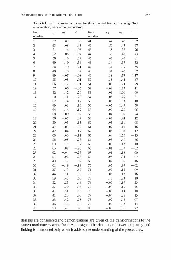
9.2 Relating Results from Different Test Forms 287
Table 9.4 Item parameter estimates for the simulated English Language Testafter rotation, translation, and scaling
Itemnumber
a1 a2 d Itemnumber
a1 a2 d
1 .67 �:03 :09 41 :44 :45 1:02
2 .63 :08 :43 42 :50 :43 :67
3 .71 �:14 �:08 43 :38 :32 :76
4 .52 :06 �:04 44 :39 :45 :43
5 .58 :16 :34 45 :42 :45 :81
6 .69 �:19 �:36 46 :34 :37 :52
7 .54 �:10 �:21 47 :34 :39 :55
8 .48 :10 :07 48 :51 :40 :92
9 .69 �:05 �:08 49 :38 :53 1:17
10 .55 :08 :01 50 :38 :44 :67
11 .66 �:12 �:01 51 :09 1:24 :29
12 .57 :06 �:06 52 �:09 1:23 :11
13 .52 :12 :20 53 :01 1:01 �:0014 .50 :11 �:29 54 :08 1:29 �:3115 .62 :14 :12 55 �:08 1:33 :10
16 .49 :08 :10 56 �:05 1:49 :38
17 .64 :14 �:12 57 �:00 1:29 :05
18 .68 �:09 �:02 58 :04 1:05 :24
19 .56 �:07 :04 59 �:02 :94 :12
20 .59 �:03 :15 60 :05 1:11 :08
21 .47 �:03 �:02 61 �:02 1:15 :16
22 .42 �:04 :17 62 :06 1:00 :12
23 .68 :06 �:11 63 :04 1:20 �:1324 .58 �:05 �:28 64 �:08 1:49 :66
25 .69 �:18 :07 65 :00 1:17 :10
26 .65 :02 �:20 66 �:01 1:00 �:0227 .62 �:04 �:27 67 :01 1:13 :00
28 .51 :02 :28 68 �:05 1:34 :07
29 .49 :17 :32 69 �:02 1:06 :16
30 .61 �:19 �:18 70 :03 :95 �:0231 .37 :43 :67 71 �:09 1:18 :09
32 .44 :21 :39 72 :05 1:17 :16
33 .59 :45 :60 73 :13 1:23 :10
34 .52 :23 :44 74 �:05 1:17 :23
35 .37 :39 :33 75 �:00 1:19 :45
36 .41 :51 :63 76 �:03 1:14 :18
37 .41 :20 :30 77 �:04 1:26 :15
38 .33 :42 :78 78 :02 1:46 :07
39 .46 :38 :62 79 :02 1:02 �:1440 .53 :45 :80 80 �:03 1:01 :22
designs are considered and demonstrations are given of the transformations to thesame coordinate systems for these designs. The distinction between equating andlinking is mentioned only when it adds to the understanding of the procedures.

288 9 Linking and Scaling
–1.2 –1 –0.8 –0.6 –0.4 –0.2 0 0.2 0.4 0.6 0.8–1.5
–1
–0.5
0
0.5
θ1
θ 2
Fig. 9.4 Item arrows for the simulated English test after rotation, translation, and scaling
The three designs that are considered here are: the common-person design; thecommon-item, nonequivalent-groups design (also called the nonequivalent groupanchor test (NEAT) design); and the randomly equivalent-groups design. Thecommon-person design develops the transformation to the same coordinate systemfrom the responses from a set of persons who take both test forms. No test items arein common between the test forms. The common-item nonequivalent-groups designdevelops the transformation to the same coordinate system from the calibration ofthe same set of items in both test forms. The randomly equivalent-groups designuses common reference composites for the tests and the assumption that the originof the space is in the same location because the groups of examinees are randomlyequivalent.
9.2.1 Common-Person Design
Suppose that a testing program has two forms of a test and would like to reportthe results of the tests within the same multidimensional framework. The goal isto put the ™-estimates from the two tests into the same coordinate system. One ap-proach to doing this is to administer both test forms to a sample of examinees underconditions where it can be assumed that no change has occurred to the examineesbetween the administrations of test forms. The two test forms may be administeredin counterbalanced order to control for fatigue or familiarity effects.

9.2 Relating Results from Different Test Forms 289
Because the examinees are assumed to be unchanged for the two test adminis-trations, their relative locations in the ™-space should be the same. Any observeddifferences in location should be because of the arbitrary setting of origin, rotationof axes, and units on the coordinate axes. If a transformation can be identified thatconverts the locations of the examinees from the calibration of one test into the lo-cation from the calibration of another test, then that same transformation can beused to place the ™-points for all examinees taking the second test into the ™-spacedefined by the first test. Functions of the transformation of the ™s can also be usedto put the item parameters into the same framework as the initial test.
For the example given here, the ™-space defined at the end of Sect. 9.1 will beconsidered as the results from the base form and the goal will be to transform the re-sults from a second test form built to the same test specifications to this coordinatesystem. A random sample of 200 examinees from the calibration population for thefirst test form is administered the second test form along with the regular calibra-tion sample for that form of 6,000. The sample of 6,000 may not be from the samepopulation as the sample used to calibrate the first test form. Overall, the calibrationsample for the second test is 6,200. This sample size should give item parametersthat are well estimated, but the coordinate system defined by the second calibrationis not expected to be equivalent to that defined by the calibration of the first testform. The results of the calibration of the items for the second test form are given inTable 9.5. The arrow plot based on the item parameter estimates is given in Fig. 9.5.A comparison of the item parameter estimates and the arrow plot for Form 2 to thosefrom the initial form show that they have a very similar pattern, but they are not ex-actly the same. The results shown here are similar to those that would be obtainedfrom careful construction of test forms to the same table of specifications.
The sample size of 200 used in the example was chosen for convenience. Thisshould not be taken as a recommendation for the sample size for a common-persondesign. There is no research at this time that has investigated the size of sam-ple needed for a common-person design. If the locations of the examinees wereestimated without error, only a small number of examinees would be needed to de-termine the transformation. However, TESTFACT reports that the standard errorsfor the estimates of the coordinates for the examinee locations are in the range from.3 to .5 so a reasonably large sample size is needed to compensate for error in esti-mation when determining the transformation. A sample size of 200 was selected inthis case because that number results in fairly good estimates of correlations.
Once the ™-estimates are obtained for the common examinees, the proceduresdescribed in Chap. 8 are used to determine the transformation that will minimize thesquared difference in the locations of the individuals. The first step is to subtractthe vector of the means of the coordinates from each of the coordinate vectors forthe common examinees. Then a nonorthogonal Procrustes rotation is determinedfor rotating the estimates of the common persons’ locations from the second test tomatch the same persons’ locations in the base coordinate system (i.e., the coordinatesystem after aligning the reference composites to the axes and changing the originand units). This methodology was described in Sect. 8.2.1.

290 9 Linking and Scaling
Table 9.5 TESTFACT item parameter estimates for the simulated EnglishLanguage Test Form 2
Itemnumber
a1 a2 d Itemnumber
a1 a2 d
1 .60 .21 .21 41 .55 .25 :53
2 .64 .22 .30 42 .50 .37 :98
3 .77 .20 .44 43 .67 .28 :85
4 .67 .20 .20 44 .63 .46 :69
5 .71 .13 .50 45 .67 .36 :91
6 .67 .11 .50 46 .79 .53 :83
7 .42 .08 .19 47 .47 .36 :44
8 .63 .24 .29 48 .71 .32 :88
9 .88 .25 .37 49 .46 .37 :69
10 .83 .09 .57 50 .83 .41 1:35
11 .78 .17 .78 51 .28 .63 �:2912 .62 .07 .28 52 .23 .60 �:5813 .92 .13 .79 53 .23 .66 �:4214 .79 .24 .04 54 .13 .58 �:5315 .57 .17 .32 55 .21 .72 �:5316 .61 .10 .34 56 .24 .76 �:3917 .56 .14 .37 57 .29 .78 �:0418 .85 .19 .23 58 .30 .82 :11
19 .74 .17 .25 59 .25 .50 �:1120 .91 .28 .36 60 .18 .96 �:4721 .84 .31 .50 61 .10 .57 �:1522 .73 .15 .59 62 .22 .62 �:4123 .83 .21 .46 63 .18 .81 �:4724 .73 .18 .49 64 .29 .70 �:4125 .59 .17 .45 65 .23 .82 �:0126 .86 .34 .74 66 .12 .54 �:2527 .79 .19 .58 67 .12 .72 �:4628 .90 .25 .51 68 .26 .64 �:5429 .91 .11 .34 69 .22 .65 �:4530 .68 .19 .50 70 .21 .58 �:4031 .64 .40 .85 71 .21 .74 �:4832 .55 .42 .96 72 .20 .55 �:2333 .64 .47 .82 73 .20 .60 �:2834 .66 .34 .88 74 .20 .69 �:5135 .65 .43 .53 75 .10 .56 �:3036 .68 .33 .42 76 .29 .80 �:4237 .67 .34 .75 77 .17 .57 �:2738 .72 .35 .94 78 .13 .73 �:4639 .59 .37 .91 79 .28 .73 �:6440 .55 .41 .77 80 .18 .71 �:30

9.2 Relating Results from Different Test Forms 291
–1 –0.5 0 0.5 1 1.5
–1
–0.5
0
0.5
1
1.5
θ1
θ 2
Fig. 9.5 Item arrows for the simulated English Language Test Form 2
In this case, the transformation matrix, labeled M�1 in (8.24), is
�1:0992 :2089
:2722 :5530
�:
This matrix is the equivalent of RotC in (9.1). It is a fairly close match to thatterm, but it is not exactly the same. The differences are because of a combinationof estimation error in the locations of the 200 common persons and differencesbetween the first and second test forms.
The transformation matrix given earlier only accounts for the difference in theorientation of the coordinates axes between the TESTFACT calibration results andthe base coordinate system that was developed earlier in this chapter. There is also aneed to shift the origin from the results of the TESTFACT calibration to the origin ofthe base coordinate system. The expression for the shift in origin is given in (8.26).For the data used in this example, the value of k is given by
k D N™base � N™Form2 M�1
D �:5385 �:4301 � � ��:0411 :0125
� � 1:0992 :2089
:2722 :5530
�(9.4)
D �:5802 �:4285 � :
The vector obtained here can be compared to the shift in origin from the originaltransformation to the base coordinate system given in (9.1). Note that the signs are

292 9 Linking and Scaling
different because in (9.1) the vector is subtracted while in determining k the termsare summed. The complete transformation for the ™-estimates from the second testis given by
O™base D O™Test
�1:0992 :2089
:2772 :5530
�C Œ:5802 � :4285 : (9.5)
As with the original transformation to the base coordinate system, the item pa-rameters from the second test need to be transformed to the base coordinate systemto maintain the invariance properties of the MIRT model. The a-parameter vectorsmust be multiplied by the transpose of the inverse of the multiplier of the ™-estimatesfrom the second test. That is,
Oabase D OaTest2�M�1�10 D OaTest2M0 D OaTest2
�1:0036 �:4940�:3792 1:9950
�: (9.6)
Similarly, the d -parameter for each item needs to be transformed to the base coor-dinate system. This transformation is given by
Odbase D OdTest2 � OaTest2M0k0: (9.7)
The results of the transformation of the item parameter estimates from the cal-ibration of test Form 2 to the base coordinate system are given in Table 9.6 andFig. 9.6. These results can be compared to those from the conversion of the calibra-tion of the initial form to the base coordinate system. As with the initial conversionof Form 1 to the base coordinate system, the a2-parameter estimates for the first 30test items are now near zero with some negative. Similarly, for the last 30 test items,the a1-parameter estimates are near zero. The item arrows in Fig. 9.6 show the ori-entation of the two item sets along the coordinate axes. This plot can be compared toFig. 9.4 to determine the similarity of the solutions after they have been transferredto the base coordinate system.
9.2.2 Common-Item Design
Although the common-person design is conceptually straight forward, it is not usedvery often for operational linking and equating. There is usually some concern thatthe examinees will not be equally motivated when responding to the two test formsand counterbalancing the administration of the test forms may not be sufficientto balance differences in motivation. There may also be other types of carry-overeffects, such as experience taking the test or fatigue effects, that may affect thecomparability of performance on the two test forms. There may also be difficul-ties recruiting a sufficient size examinee sample to take both test forms. For thesereasons other equating designs are more often implemented.

9.2 Relating Results from Different Test Forms 293
Table 9.6 TESTFACT item parameter estimates for the simulated English Lan-guage Test Form 2 after rotation, translation, and scaling to the base coordinatesystem using the common-person approach
Itemnumber
a1 a2 d Itemnumber
a1 a2 d
1 .52 :13 �:03 41 :46 :23 :37
2 .56 :13 :03 42 :36 :49 :98
3 .70 :02 :04 43 :56 :23 :62
4 .59 :08 �:11 44 :46 :60 :68
5 .67 �:10 :07 45 :54 :39 :77
6 .63 �:10 :09 46 :59 :67 :77
7 .39 �:05 �:06 47 :34 :48 :45
8 .54 :17 :05 48 :59 :29 :67
9 .79 :06 �:07 49 :32 :52 :73
10 .79 �:22 :02 50 :68 :40 1:12
11 .73 �:05 :33 51 :04 1:13 :17
12 .59 �:16 �:13 52 :00 1:08 �:1213 .87 �:20 :20 53 �:02 1:20 :11
14 .70 :10 �:32 54 �:09 1:10 �:0115 .51 :05 :05 55 �:06 1:34 :08
16 .57 �:09 �:03 56 �:05 1:40 :24
17 .51 �:00 :07 57 �:01 1:41 :56
18 .78 �:04 �:24 58 �:01 1:48 :76
19 .68 �:03 �:16 59 :06 :87 :22
20 .81 :12 �:06 60 �:18 1:83 :42
21 .72 :21 :17 61 �:11 1:08 :37
22 .68 �:07 :17 62 �:02 1:14 :09
23 .75 :00 :03 63 �:12 1:52 :26
24 .67 �:00 :10 64 :02 1:26 :12
25 .53 :04 :16 65 �:08 1:52 :69
26 .74 :25 :41 66 �:08 1:01 :23
27 .72 �:01 :15 67 �:15 1:38 :22
28 .80 :06 :07 68 :02 1:14 �:0629 .88 �:23 �:22 69 �:02 1:19 :07
30 .61 :05 :17 70 �:01 1:06 :06
31 .49 :48 :77 71 �:07 1:38 :16
32 .39 :57 :98 72 �:01 1:00 :21
33 .47 :62 :80 73 �:02 1:09 :20
34 .53 :35 :73 74 �:06 1:27 :07
35 .49 :54 :47 75 �:11 1:06 :22
36 .56 :33 :24 76 �:01 1:46 :21
37 .54 :35 :58 77 �:04 1:05 :21
38 .59 :35 :75 78 �:14 1:39 :22
39 .45 :45 :84 79 :01 1:31 �:0940 .40 :54 :77 80 �:09 1:32 :32
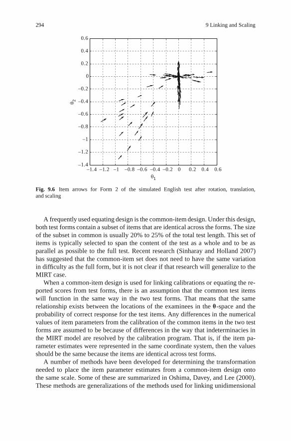
294 9 Linking and Scaling
–1.4 –1.2 –1 –0.8 –0.6 –0.4 –0.2 0 0.2 0.4 0.6–1.4
–1.2
–1
–0.8
–0.6
–0.4
–0.2
0
0.2
0.4
0.6
θ1
θ 2
Fig. 9.6 Item arrows for Form 2 of the simulated English test after rotation, translation,and scaling
A frequently used equating design is the common-item design. Under this design,both test forms contain a subset of items that are identical across the forms. The sizeof the subset in common is usually 20% to 25% of the total test length. This set ofitems is typically selected to span the content of the test as a whole and to be asparallel as possible to the full test. Recent research (Sinharay and Holland 2007)has suggested that the common-item set does not need to have the same variationin difficulty as the full form, but it is not clear if that research will generalize to theMIRT case.
When a common-item design is used for linking calibrations or equating the re-ported scores from test forms, there is an assumption that the common test itemswill function in the same way in the two test forms. That means that the samerelationship exists between the locations of the examinees in the ™-space and theprobability of correct response for the test items. Any differences in the numericalvalues of item parameters from the calibration of the common items in the two testforms are assumed to be because of differences in the way that indeterminacies inthe MIRT model are resolved by the calibration program. That is, if the item pa-rameter estimates were represented in the same coordinate system, then the valuesshould be the same because the items are identical across test forms.
A number of methods have been developed for determining the transformationneeded to place the item parameter estimates from a common-item design ontothe same scale. Some of these are summarized in Oshima, Davey, and Lee (2000).These methods are generalizations of the methods used for linking unidimensional

9.2 Relating Results from Different Test Forms 295
IRT calibrations. Among them are generalizations of the Stocking and Lord (1983)and the Haebara (1980) methods. Oshima, Davey, and Lee (2000) evaluated thesedifferent methods, but only considered a two-dimensional case. It is not clear thatthe results would generalize to item response data modeled using more than twodimensions. It is clear that more research is needed to investigate the functioning ofmethods for putting calibrations into the same coordinate system when the common-item design is used.
To demonstrate the use of the common-item design in this section, the two testforms from the previous section are used. As before, the initial test form is usedto set the base coordinate system for the testing program. Sixteen test items arerandomly selected from the 80 in the test form to produce the common-item linkbetween the two calibrations. Six test items were selected from the first 30 items,four test items from the next 20 items, and six test items from the last 30 items. Thisstratified selection process insured that the common-item set would represent thethree constructs that were the focus of the test.
The second test form is modified for this demonstration by replacing the corre-sponding items in that form with the common items selected from the first form. Theitem parameter estimates from the first form after transformation to the base coor-dinate system are the target for the transformation. The goal of the linking/equatingis to find the transformation that will convert the item parameter estimates from thesecond test form to be as close as possible to those in the base coordinate system.Table 9.7 lists the item numbers for the common items, the item parameter estimatesin the base coordinate system and the item parameter estimates from the calibrationof Form 2 based on a sample of 6,000 examinees.
Table 9.7 Item parameter estimates for the common items from the basecoordinate system and from the initial calibration of Form 2
Itemnumber
Base calibration Form 2 calibrationa1 a2 d a1 a2 d
3 :71 �:14 �:08 .82 .17 :40
6 :69 �:19 �:36 .74 .74 :18
8 :48 :10 :07 .66 .17 :38
16 :49 :08 :10 .59 .20 :33
18 :68 �:09 �:02 .77 .15 :45
21 :47 �:03 �:02 .58 .13 :29
37 :41 :20 :30 .54 .26 :47
44 :39 :45 :43 .55 .38 :48
45 :42 :45 :81 .55 .42 :86
49 :38 :53 1:17 .54 .45 1:17
63 :04 1:20 �:13 .26 .72 �:6370 :03 :95 �:02 .16 .62 �:4271 �:09 1:18 :09 .12 .74 �:5072 :05 1:17 :16 .29 .72 �:3377 �:04 1:26 :15 .18 .70 �:3979 :01 1:02 �:14 .20 .64 �:56

296 9 Linking and Scaling
The transformation from the Test 2 item parameter estimates for the com-mon items to the item parameter estimates on the base coordinate system canbe determined from the equations given in Chap. 8. The rotation and scaling ofthe a-parameters is given by (8.31). The matrix determined by this equation is thenonorthogonal Procrustes rotation of the Test 2 a-parameter estimates to the basecoordinate system a-parameters. For the common items given in Table 9.7, the trans-formation matrix for the a-parameters is
�:9140 �:4705
�:2674 1:7781
�:
The matrix of a-parameters from Test 2 is postmultiplied by this matrix to put theparameters onto the scale of the base coordinate system. The transpose of the in-verse of this matrix can be used to transform the ™-estimates after they have beentranslated to have a mean of 0. The matrix given earlier is comparable to the result of(9.6) for the common-person method of linking calibrations. These matrices are notthe same because the two methods are minimizing different errors. The common-person method is minimizing differences in person locations. The common-itemmethod is minimizing errors in item parameters.
The conversion of the d-parameters from the common items to the base coordi-nate system is done using (8.33). The a-parameters in that equation are those in thebase coordinate system. The value of � is determined from (8.34) using the itemparameter estimates from the items that are common to the two test forms. For theitem parameter estimates given in Table 9.7, � is
�:6285
�:4363�:
Once these two conversion equations have been determined, the full set of itemparameters from Test 2 can be converted to the base coordinate system. There is onecomplication in the use of (8.33). Test Form 2 does not have a-parameters for thenoncommon items from the base coordinate system. Therefore, the a-parameters forthe full Form 2 must first be converted to the base coordinate system as describedearlier, and then the converted a-parameters are used in (8.33). The result of theapplication of (8.33) to the d-parameters is given in Table 9.8.
The results of the transformation of the item parameters from the Test 2 calibra-tion to the base coordinate system can be checked by comparing the item parameterestimates from the common items after transformation with the values from the cali-bration in the base coordinate system. For example, the parameter estimates for Item49 in the base coordinate system were Œ:38 :53 1:17. The results from the Test 2 cal-ibration after transformation are Œ:37 :54 1:17, an extremely close match. Not all ofthe pairs of parameter estimates were this close, but the overall match in this exam-ple is very good.

9.2 Relating Results from Different Test Forms 297
Table 9.8 Test 2 item parameter estimates for the simulated English LanguageTest Form 2 after rotation, translation, and scaling to the base coordinate systemusing the common-item approach
Itemnumber
a1 a2 d Itemnumber
a1 a2 d
1 .49 :03 �:04 41 :44 :28 :36
2 .56 :03 �:03 42 :38 :49 1:00
3 .70 �:08 �:08 43 :51 :22 :58
4 .60 �:05 �:17 44 :41 :41 :40
5 .62 �:12 :09 45 :39 :49 :82
6 .65 �:14 �:29 46 :55 :59 :72
7 .37 �:10 �:07 47 :34 :44 :44
8 .56 �:00 :03 48 :53 :31 :67
9 .75 �:06 �:12 49 :37 :54 1:17
10 .65 �:14 :13 50 :62 :31 1:08
11 .64 �:09 :32 51 :08 :91 :05
12 .49 �:08 �:04 52 :06 :91 �:2213 .76 �:21 :22 53 :03 1:11 :06
14 .69 �:01 �:39 54 �:02 1:07 �:0415 .47 :02 :04 55 :03 1:16 �:0016 .48 :08 :06 56 :02 1:24 :12
17 .47 �:03 :06 57 :04 1:25 :45
18 .65 �:09 �:00 58 :02 1:39 :70
19 .57 �:07 �:13 59 :04 :82 :17
20 .69 :10 �:01 60 �:04 1:48 :25
21 .49 �:04 �:04 61 �:04 :91 :27
22 .60 �:06 :15 62 :02 1:14 :05
23 .67 �:02 :00 63 :05 1:15 �:1524 .57 �:03 :14 64 :08 1:12 :04
25 .52 �:05 :09 65 �:05 1:43 :65
26 .65 :14 :35 66 �:02 :92 :18
27 .64 �:08 :09 67 �:06 1:09 :07
28 .80 �:08 �:02 68 :03 1:09 �:1029 .77 �:13 �:12 69 :05 1:00 �:0430 .59 �:04 :14 70 �:02 1:03 :05
31 .44 :41 :72 71 �:08 1:26 :10
32 .42 :46 :89 72 :07 1:14 :12
33 .47 :59 :81 73 �:00 :99 :19
34 .49 :30 :72 74 �:03 1:21 :04
35 .49 :52 :45 75 �:06 :97 :12
36 .50 :26 :20 76 �:00 1:32 :12
37 .42 :21 :30 77 �:03 1:17 :13
38 .53 :39 :81 78 �:12 1:31 :18
39 .44 :35 :80 79 :02 1:04 �:1240 .39 :44 :72 80 �:02 1:10 :26

298 9 Linking and Scaling
After the item parameter estimates from the test have been converted to the basecoordinate system, the transformation of the ™-vectors can be determined. The trans-formation is derived by noting that the values of the exponents of the model forthe items must remain the same for the invariance property of the MIRT model tohold. Using the notation that ab represents the item discrimination parameters aftertransformation to the base coordinate system, a2 represents the item discriminationparameters for the same items from the initial calibration of Test 2, db and d2 are thecorresponding intercept terms, ™ is the matrix of coordinates in the base coordinatesystem for the examinees used in the calibration, and � is the matrix of coordinatesfor the calibration sample from the Test 2 calibration, the transformation of the Test2 person parameters, �, to the base coordinate system is given in (9.8).
ab™0 C db1 D a2�0 C d21;
ab™0 D a2�0 C d21 � db1;
a0bab™
0 D a0b
�a2�0 C .d2 � db/ 1
�; (9.8)
�a0
bab�1
a0bab™0 D �
a0bab�1
a0b
�a2�0 C .d2 � db/ 1
�;
™0 D �a0
bab�1
a0ba2�0 C �
a0bab�1
a0b .d2 � db/ 1:
The last line of (9.8) has the nonorthogonal Procrustes rotation to a target ofa2 as the multiplier of �. This is the opposite of the rotation of the a2-parametersthat has a target of the rotation of ab. The term on the right of the last line is thesame as (8.34). The equation in the last line of (9.8) can only be used after the itemparameter estimates have been transformed from the Test 2 calibration to the basecoordinate system. At that time, all of the values needed in the equation are availableand the estimates of location in the space defined by the calibration of Test 2 canbe transformed to locations in the base coordinate system.
9.2.3 Randomly Equivalent-Groups Design
The randomly equivalent-groups design is used with some frequency for equatingwhen tests are assumed to be sensitive to differences in examinee performance ona single composite of skills. The examinee sample is randomly divided into two ormore subsamples with the number of samples equal to the number of test forms tobe equated. The assumption is that the distribution of performance on the compositeof skills being assessed should be the same across samples because of the randomassignment of forms to samples and any differences in distributions are because ofslight differences in the characteristics of the tests. Transforming the scores fromthe different forms of the tests to a common scale involves determining the transfor-mation that will yield distributions with the same features for all test forms. Lineartransformations and the equipercentile method are often used with the randomlyequivalent-groups design (see Kolen and Brennan 2004).

9.2 Relating Results from Different Test Forms 299
The randomly equivalent-groups design is effective because carefully con-structed test forms can be assumed to result in score scales that have the sameconceptual meaning. That is, the construct that is represented by the test scores isthe same across all forms. Also, the distributions of performance are assumed to bethe same because of the random assignment to groups. With sufficient sample size,there is statistical justification for the assumption of a common distribution.
The use of the randomly equivalent-groups design for the multidimensional casehas an additional complication over the unidimensional application because the ori-entation of the coordinate axes might not be the same for the calibration of two testforms even when the examinee groups are random samples from the same popula-tion. Also, there are no common test items that can be used to determine the rotationneeded to align the coordinate axes. The use of randomly equivalent groups in themultidimensional case requires developing a criterion for rotating the coordinateaxes to a common orientation.
Future work in MIRT will no doubt come up with other ways of solving thisproblem, but here the solution is determined from the reference composites for theconstructs assessed by the tests. As with the unidimensional case, it is assumed thatthe test forms were constructed to be parallel, or at least be measuring common con-structs. If those constructs can be identified for both test forms, then the coordinateaxes can be transformed to a common orientation by finding the rotation that willalign the reference composites from the tests.
This approach to equating or linking MIRT calibrations has the following steps:
1. For a test with parameters in the base coordinate system, determine the sets oftest items that best measure each of the reference composites. A transformationto the base coordinate system should already be available for this test form.
2. Administer the base test, Test 1, and the new test, Test 2, to randomly eqivalentgroups of examinees.
3. Calibrate Test 1 using this sample and determine the directions of the refer-ence composites in the coordinate space. The direction cosines of the referencecomposites are used as the a-parameters for the reference composites. Theyare collected together into a matrix that will be used as the target to determinethe rotation for the calibration results from Test 2.
4. Calibrate Test 2 using a sample of examinees that is randomly equivalent to thesample for the base test.
5. Using procedures like the cluster analysis described in Sect. 8.3, determine thesets of items that correspond to the reference composites from Test 1.
6. Determine the directions of the reference composites for Test 2 and compute thereference composite a-matrix for Test 2.
7. Determine the nonorthogonal procrustes rotation that will convert the directionsof the reference composites in Test 2 to the directions of the reference compositesfor Test 1.
8. The rotation matix can be used to convert all of the a-parameters on Test 2 tothe coordinate system for Test 1. The inverse rotation can be used to convert thelocation parameters from Test 2.

300 9 Linking and Scaling
After the rotation of the item and person parameters to the Test 1 coordinatesystem, they can be transformed to the base coordinate system using the same trans-formation that was used on Test 1. Because the groups are randomly equivalent,there should be no need to change the origin and units of measurement, but if nec-essary, the same methods used in Sect. 9.2.1 can be applied.
This method of linking calibrations can be demonstrated using the two test formswith item parameter estimates given in Tables 9.1 and 9.5. These two sets of parame-ters were estimated from data generated assuming the same underlying distributionof ™. Therefore, they are equivalent to results from tests calibrated using the ran-domly equivalent-groups design.
Because this is a simulated example, the clusters of test items related to constructsare known. For real tests, the test items are intended to measure specific sets ofcontent and skills, but it is important to verify that test items measuring the sameconstructs cluster together. This can be part of the evidence for the content validityof the test.
For the simulated tests used here, the reference composites for the clusters ofitems were determined for the two test forms. The eigenvectors corresponding tothe largest eigenvalues for each construct are given in Table 9.9. After obtaining theeigenvectors for the reference composites for the two test forms, the nonorthogonalProcrustes rotation was determined for rotating the Test 2 reference composites toalign with the Test 1 reference composites. In this case, the two test forms were veryparallel in construction so the rotation was close to the identity matrix
�1:0036 �:0115�:0056 1:0080
�:
The matrix of eigenvectors from Test 2 is then postmultiplied by this rotation matrixto transform them to the same coordinate system as Test 1. This same rotation matrixwould also be applied to the a-parameter matrix from Test 2 to put the a-parametersinto the Test 1 coordinate system. After this adjustment, the same transformationthat was applied to Test 1 in Sect. 9.1 can be applied to the results for Test 2 to putthem onto the base coordinate system for the testing program.
The results presented here are much better than those obtained for operationaltests. In actual testing situations, it is difficult to identify the sets of items that arebest at measuring each reference composite and the construction of the tests will not
Table 9.9 Eigenvectors for the reference composites for Test 1, Test 2, and Test 2 after nonorthog-onal Procrustes rotation to match Test 1.
Construct Eigenvectors
Test 1 Test 2 Rotated Test 2
1 2 1 2 1 2
Reading .9741 .2262 .9700 .2429 .9722 .2337Vocabulary .8568 .5157 .8590 .5120 .8592 .5062Conversation .2898 .9571 .2933 .9560 .2890 .9603
9.3 Estimating Scores on Constructs 301
likely be as parallel as this example. The quality of the linkage of the calibrationswill depend on how well items can be connected to constructs and how well formshave been constructed.
9.3 Estimating Scores on Constructs
Many tests of cognitive abilities are purposely constructed to assess many differ-ent types of skills and content knowledge. For example, the Mathematics Test ofthe ACT college admissions test battery (ACT, Inc. 2007) includes test items thatare designed to assess prealgebra, elementary algebra, intermediate algebra, coor-dinate geometry, plane geometry, and trigonometry. When tests are constructed tocover a wide variety of skills and content, there is often a desire to report results onthe performance on the full set of test items and on the constructs defined by the sub-sets of items. The common approach to reporting results on the separate constructsin the test design is to create shorter tests from the separate sets of items relatedto each construct and develop proficiency estimates from each test item set. Thisapproach can sometimes lead to inaccurate results when the number of test itemsrelated to a construct is small. But even in those cases, there are often pressuresfrom users of the tests to report those inaccurate results.
The approach to the reporting of scores on separate constructs taken in thissection avoids the problem of using small sets of test items by not estimating pro-ficiency on those sets of items in isolation. Rather, the full set of test items is usedto estimate the location of an individual in the multidimensional space defined bythe matrix of item response data and the MIRT model. The subsets of test itemsthat are of interest for reporting results are used to define reference composites inthe same multidimensional space. Then, the reporting of results on these item setsis accomplished by mapping the estimated location of the person onto each of thereference composites. Two methods for accomplishing this mapping are presentedhere: rotation and projection. These methods are mathematically closely related, butthey are somewhat different from a conceptual viewpoint so they will be describedseparately. To make the description of the methods concrete, the first example fromthis chapter will be used to demonstrate the methods.
Suppose the test described at the beginning of this chapter was administeredto a large sample of examinees and the resulting item-score matrix was calibratedyielding the results given in Table 9.1. The constructs assessed by the test weredescribed in the test specifications and were confirmed using cluster analysis ofthe angular differences yielding the result in Figs. 9.1 and 9.2. The goal is to reportfour measures of performance on this test, a measure of overall performance and ameasure on each of the three constructs described in the test specifications – reading,vocabulary, and conversation.
The ™-vectors estimated from each person obtained from the original calibrationof the item response data do not provide any of the desired measures. The ™-vectorsdo provide estimates of the locations of the individuals in the coordinate system

302 9 Linking and Scaling
–2 –1.5 –1 –0.5 0 0.5 1 1.5 2–2
–1.5
–1
–0.5
0
0.5
1
1.5
2
θ1
θ 2
Fig. 9.7 ™-points (stars) and item arrows from the initial calibration
initially defined by the TESTFACT calibration. The demonstration given here willuse four hypothetical individuals out of the initial calibration sample to show how toderive the reported proficiency estimates. Suppose these four individuals have initial™-vectors of .1; 1/, .1; �1/, .�1; 1/, and .�1; �1/. Each of these ™-vectors fromthe initial calibration will be used to determine the levels of proficiency on each ofthe desired reporting constructs. The locations of these points are given in Fig. 9.7along with the item vectors for the test.
9.3.1 Construct Estimates Using Rotation
When determining the base coordinate system in Sect. 9.1 of this chapter, the ref-erence composites for the reading and conversation constructs were rotated to alignwith the coordinate axes. The result is that if the ™-vectors are transformed using thecorresponding rotations and translations, the new coordinates for the person loca-tions yield the estimates on two of the constructs that were targets of measurementfor this test. Part of the work of getting the estimates of proficiency can be done bytransforming the four ™-vectors to the new base coordinate system using the trans-formations given in (9.1). After this transformation, the �1 values are the estimatesof the reading construct and the �2 values are the estimates of the conversation con-struct. The location of the points for the four hypothetical individuals and the itemarrows after transformation to the base scale is shown in Fig. 9.8.

9.3 Estimating Scores on Constructs 303
–1.5 –1 –0.5 0 0.5 1 1.5 2 2.5–1.5
–1
–0.5
0
0.5
1
1.5
2
2.5
θ1
θ 2
Fig. 9.8 Locations of points (stars) and item arrows after transformation
Although the rotation of the initial calibration to align two of the constructs alongthe coordinate axes solves part of the problem, there is still the need to determinethe estimates for the vocabulary construct and the test as a whole. To do that, the ref-erence composites for the total test and the vocabulary items are needed for the finalreporting coordinate system. These can be determined using the final a-parametersshown in Table 9.4. The eigenvector for the reference composite of the vocabularyitems is Œ:73 :68. This is a direction that is 43ı from the �1-axis. If the axes arerotated around the origin 43ı in a counterclockwise direction, the �1-axis will bealigned with the reference composite for the vocabulary items. Then the coordinatesof the person locations on the �1-axis will give estimates of the proficiency on thevocabulary component of the test.
The rotation required to align the �1-axis with the vocabulary reference com-posite can be determined using (9.8) in this case because the solution is in twodimensions. The rotation matrix to align the vocabulary reference composite withthe �1-axis is �
:73 �:68:68 :73
�:
Postmultiplying the locations of persons in the space with this same matrix resultsin their locations in the rotated coordinate system. The item vector plot and thelocations of the four reference points after the rotation are shown in Fig. 9.9. Afterthis rotation, the vocabulary proficiency can be determined from the projections ofthe locations on the �1-axis.
The same process can be followed to determine the level of performance on thereference composite for the entire test. The eigenvector for the reference compositefor the full test is Œ:100 :995. This corresponds to a reference compose that is at

304 9 Linking and Scaling
–2 –1.5 –1 –0.5 0 0.5 1 1.5–2
–1.5
–1
–0.5
0
0.5
1
1.5
Vocabulary θ
θ 2
Fig. 9.9 Item arrows and locations (stars) after aligning �1 with the vocabulary referencecomposite
84ı with the �1-axis. This reference composite is closely aligned with the directionsof best measurement for the speaking items because of the rescaling that was donethat resulted in higher a-parameters for the �2-coordinate axis. Under this scaling,the total test score estimates will be highly related to the speaking construct. Thetransformation of scale resulted in a higher weighting in the reference composite ofthe speaking construct. The rotation to align the full test reference composite withthe �1-axis is
�:100 �:995:995 :100
�:
The results of the rotation are shown in Fig. 9.10. As with the previous result, thecoordinates of the locations shown by the stars on the �1-axis are now a measure ofthe proficiency of the persons on the full reference composite for the test.
9.3.2 Construct Estimates Using Projection
Another approach to obtaining estimates of the location of examinees on the con-structs defined by sets of test items is to project the locations of the examinees inthe ™-space orthogonally onto the lines for each of the reference composites for thesets of items. Using the example from the previous section, consider the locationsof the four example points in the ™-space and four reference composites for the

9.3 Estimating Scores on Constructs 305
Fig. 9.10 Rotation to alignthe �1-axis with the referencecomposite of the test
–2 –1.5 –1 –0.5 0 0.5 1 1.5–2
–1.5
–1
–0.5
0
0.5
1
1.5
Reference Composite θ
θ 2
Fig. 9.11 Reference compos-ites (solid arrows) with fourpoints in the ™-space (stars)with projections from onepoint to each of the referencecomposites (broken line ar-rows).
–2 –1.5 –1 –0.5 0 0.5 1 1.5 2–2
–1.5
–1
–0.5
0
0.5
1
1.5
2
θ1
θ 2
test – the reference composites for each of vocabulary, reading, conversation, andthe total test. The four points and the four reference composites are shown the basecoordinate system in Fig. 9.11.
Figure 9.11 shows each reference composite as an arrow and the dotted linesshow the extensions of the reference composites to the full space. The arrows drawnwith broken lines in the figure show the orthogonal projections from the .�1; 1/

306 9 Linking and Scaling
Fig. 9.12 Reference com-posites for the test and theset of vocabulary items (darkarrows) and projections froma �-point (star) to the refer-ence composites (shown bylight arrows)
–1.5 –1 –0.5 0 0.5 1 1.5 2 2.5–1
–0.5
0
0.5
1
1.5
2
2.5
3
θ1
θ 2
™-point to each of the reference composites. The remainder of this section will showhow to determine the values of the projections of the points in the ™-space ontoany line specified in the ™-space. To simplify the presentation, a two-dimensionalexample will be used to show the development of the projections, but all of themethods work equally well for projections in higher dimensions.
Reference composites are specified by vectors of direction cosines related to theangles between the coordinate axes and the line indicating the reference composite.Figure 9.12 shows the reference composites for the total test and the vocabularyitems and one ™-point at .1; 2/ in the ™-space. There is also a line in the figure fromthe origin of the space to the ™-point. This line also has angles with the coordinateaxes and corresponding direction cosines. The length of the line from the origin tothe point is given by
L Dvuut
mX
`D1�2` ; (9.9)
and the direction cosines for the line are given by
cos˛` D �`
L; ` D 1 : : :m; (9.10)
where ˛` is the angle between axis ` and the line to the ™-point. For this example,the direction cosines with the two axes are .4472 and .8944. These correspond toangles of 63ı and 27ı with the coordinate axes.
The direction cosines for the vocabulary reference composite are .7305 and .6829with corresponding angles of 43ı and 47ı with the coordinate axes. Thus, the anglebetween the line to the ™-point and the vocabulary reference composite is 20ı. The

9.3 Estimating Scores on Constructs 307
line from the origin to the ™-point, the arrow from the ™-point to the vocabulary ref-erence composite, and the line segment of the reference composite from the originto the projection for the ™-point form a right triangle. The right triangle propertiescan be used to determine the projection of the ™-point onto the reference composite.The distance from the projection of the ™-point on the vocabulary reference com-posite to the origin is simply cos 20ıp
12 C 22 D 2:1. A similar approach can betaken for the reference composite for the full test. The difference in angles is 21ıand the distance of the projection on that reference composite from the origin is alsoabout 2.1.
This process of projection onto a reference composite for ™-points can be donein matrix terms for all of the estimated ™s in a sample. The vector of distances ofthe ™-points from the origin, L, is given by
L Dq
diag�™™0; (9.11)
and the direction cosines for each point are determined by dividing each set of co-ordinates, �j by the corresponding element of L, Lj .
cos ’j D ’j
Lj: (9.12)
The cosine of the angle between the line from the origin to the ™-point and the di-rection of the reference composite can be found by the inner product of the directioncosines from (9.12) and those for the reference composite, cos ’rc. If A is the fullmatrix of angles between the lines from the origin to each ™-point, then the directioncosines for the angles between these lines and the line for each reference composite,A� rc, is given by (see (7.30) in Chap. 7)
cos A� rc D cos A cos ’0rc: (9.13)
The projection of each ™-point onto each reference composite is then given by
RCj D Lj cos ˛j;�rc (9.14)
where RCj is the projection on the reference composite for person j and cos ˛j;�rc
is the j th element of cos A� rc.The projections onto each of the reference composites from the simulated lan-
guage test were determined for each of the four example ™-points used in theprevious section. The results are presented in Table 9.10. These projections givethe same results as the rotation method used in the previous section.
While the projection and rotation methods for determining estimates on the ref-erence composites yield the same results, the projection method is much moreconvenient. A number of reference composites can be specified as rows in a ma-trix of direction cosines and a matrix of ™-values can be projected on each of thereference composites in one operation. The concept of reference composite and the

308 9 Linking and Scaling
Table 9.10 Projections of the four ™-points onto each of the reference composites
�1 �2 Reference compositeTotal Reading Vocabulary Speaking
1 1 1:09 :99 1:41 1:00
1 �1 �:90 1:01 :05 �1:00�1 1 :90 �1:01 �:05 1:00
�1 �1 �1:09 �:99 �1:41 �1:00
projection method provide a practical way for computing subscores from an MIRTanalysis. Meaningful subscores can be identified by finding sets of items that bestmeasure in approximately the same direction in the multidimensional space. Ref-erence composites can be determined for these sets of items. Then, each ™-pointcan be projected onto as many reference composites as have been identified. Thegoal for the testing enterprise is to accurately estimate the location of the personin the ™-space. With an accurate estimate of ™, results on specific composites ofcoordinates can easily be determined.
9.4 Summary and Discussion
This chapter provides a set of tools for reporting the results of MIRT analyses of theitem-score matrices from tests. First, methods are provided for configuring a ™-spacefor reporting results. This ™-space need not be the one that is the default given by acalibration program. The initial calibration can be rotated, translated, and scaled togive a more useful solution. In the example provided in the Sect. 9.1 , the solutionwas rotated so that the coordinate axes aligned with two of the constructs beingmeasured by the test. The result of that rotation is that the values of the coordinatesfor ™-points correspond to measures of the selected constructs. The calibrations werealso scaled to yield the size of units desired for each coordinate axis.
The second section of this chapter, Sect. 9.2, shows how to link the results of cal-ibrations from different tests. This is a necessary step if the results of the tests are tobe reported in a way that has common meaning. Linking calibrations is also neededwhen large sets of test items are needed with comparable item parameter estimates.This is the case for banking test items for use in later test construction and for the de-velopment of item pools for CATs. A number of methods for linking calibrations areprovided, but the common-item item design is the most commonly used. As MIRTapplications become more common, it is likely that additional linking methods willbe developed.
The procedures for linking calibrations and equating tests are essentially thesame, but equating places much stronger requirements on the process. For estimatesof persons’ locations from different test forms that have had item parameter esti-mates transformed to the same ™ coordinate system to be considered equated, theestimates must have the same error in every direction in the space. This places very

9.5 Exercises 309
strong requirements on creating parallel test forms. While it is theoretically possi-ble to perform multidimensional equating using MIRT models, there has been littleresearch that shows that the results meet the theoretical requirements for equating.This is an interesting area for future research.
Section 9.3 showed how to determine estimates of proficiency on composites ofthe coordinate axes. These composites are typically specified by selecting subsetsof test items and determining the direction of best measurement for the set. Thisdirection is called the reference composite for the set. The methodology for gettingestimates on the composite is very general, however. Users can specify any directionin the space and get estimates of performance on the composite that corresponds tothat direction by either rotating a coordinate axis to align with that direction, orprojecting onto a line in that direction. These methods provide very powerful toolsfor subscore reporting. The methods shown here are different than those that fita unidimensional IRT model to the subsets of test items in that information fromall test items are used to estimate ™. All of that information is used to estimatethe location on the reference composite rather than only the information from thelimited set of items.
MIRT procedures for linking calibrations, equating test forms, and reporting ex-aminee scores are still very much in development. It will be interesting to track howthese methods are refined through future research.
9.5 Exercises
1. The randomly equivalent-groups method of linking MIRT calibrations and per-son locations is based on some strong assumptions about the examinee samples andthe characteristics of the test forms. List the assumptions and indicate how the re-sults of the linking will likely be affected if the assumptions do not hold.
2. Specify your own desired orientation for the item calibration results given inTable 9.1. Develop a rotation matrix, translation constants, and scaling constants andapply them to the item parameters. Also, transform two or three ™ vectors. Show thatthe probability of correct response to one of the test items stays the same before andafter the transformation.
3. After the calibration of a set of test items in a two-dimensional ™-space, theangle between the reference composites for two sets of test items is 45ı. The corre-lation between the coordinates for the ™-points for this calibration is 0.0. The resultswere then rotated to align the two reference composites with the coordinate axesso that the angle between them is 90ı. What will be the correlation between the™-coordinates if they are transformed to maintain the invariance properties of themodel?
4. Discuss the results presented in Figs. 9.1 and 9.2. Identify the clusters that corre-spond to the sets of item vectors. Explain how the horizontal lines in the dendrogramrelate to the orientation of the item vectors in Fig. 9.1.

310 9 Linking and Scaling
5. The vocabulary projection in Table 9.10 yields a larger value for the ™-point.1; 1/ than for the projections on the other reference composites. Explain why thatis the case. Can this result be interpreted that the person at .1; 1/ is more proficientin vocabulary than on the other reference composites? Explain why you think youranswer is correct.
6. A reference composite for one of the constructs measured by the items on a testhas direction cosines Œ:53 :59 :08 :60. The estimated location in the ™-space foran examinee is Œ�:4 �1:7 :1 :3. What is the estimated location on the line definedby the reference composite for this examinee?
7. For the point at .�1;�1/ in Fig. 9.11, draw the projection arrows to each ofthe reference composites for the example test. What is the estimate on each of thereference composites for a person located at this point?
8. List the assumptions required by the use of the randomly equivalent-groups de-sign for linking MIRT calibrations and putting ™-estimates into a common ™-space.Suppose one test form does not include any test items sensitive to differences ona construct that is well measured by the items on the other test form. Discuss theproblems that are likely to occur if an attempt is made to link the calibrations fromthese two tests.
9. An examinee has a ™-estimate of .�1:1; 1:2/ on Form 2 of the test used inSect. 9.2.2. What is the ™-estimate on the base form for this examinee?
10. The ™-space defined by one test form is transformed to align with the ™-spacefor another test form using the common-person, nonequivalent-groupsdesign. Whenthis design is used, the ™-estimates after transformation for the two test forms areusually not exactly the same. Explain why that is the case. Suggest a statistic thatwould be useful for indicating the level of similarity of the locations of persons afterthe transformation to a common coordinate system.
11. Refer to the item parameter estimates given in Table 9.5. Assuming that theexaminee population has a standard bivariate normal distribution of ™ with meanvector 0 and the identity matrix for the variance–covariance matrix, what is the itemnumber for the easiest item on the test? Explain how you identified this test item.What test item is most sensitive to differences on the vocabulary construct? Again,explain how you identified that test item.

Chapter 10Computerized Adaptive Testing Using MIRT
Computerized adaptive testing (CAT) is a methodology for constructing a test,administering it to an examinee, and scoring the test using interactive computertechnology. This methodology has a history that is as long as that of interactivecomputing. An early summary of CAT methods is given in Weiss (1974). A de-tailed description of the development of an operational application for the ArmedServices Vocational Aptitude Battery is given in (Sands 1997). There are also sev-eral books available that describe the basic components of CAT procedures (Wainer,Dorans, Flaugher, Green, Mislevy, Steinberg and Thissen 1990; Parshall, Spray andDavey 2002; van der Linden and Glas 2000) so the basic details of the methodologyare not presented here. A review of that literature will show that most of the currentCAT methodology is based on the assumption that a unidimensional IRT model ac-curately represents the interaction between persons and test items. In this chapter,the generalization of the CAT methodology to the multidimensional case is consid-ered. To provide a framework for this material, a brief summary of the conceptualbasis for CAT is provided.
10.1 Component Parts of a CAT Procedure
In the most general case, a computerized adaptive test (also abbreviated as CAT)has a small number of component parts and procedures. The first is a set of testitems that are available for use on the test. These are either a preexisting set of testitems that have been calibrated using an IRT model and that have calibrations in thesame coordinate system, or a set of test items generated by computer software tohave specific item parameters based on an IRT model. The former of these two op-tions is the most commonly used so it will be the approach assumed in this chapter.The collection of test items stored in computer media with their item parameters isusually called an item bank or item pool, but creative psychometricians have alsoused terms such as “item vat” to indicate very large collections of test items. Becauseit is necessary to keep the computer storage of the test items secure and because theCAT methodology will withdraw the items from the computer storage for use, theterm “item bank” is used in this chapter.
M.D. Reckase, Multidimensional Item Response Theory, Statistics for Socialand Behavioral Sciences, DOI 10.1007/978-0-387-89976-3 10,c� Springer Science+Business Media, LLC 2009
311

312 10 Computerized Adaptive Testing Using MIRT
Most CAT procedures have the goal of selecting a set of test items for administra-tion to an examinee that will give information that can be used to accurately locatethe examinee within a ™-coordinate system. Thus, a major component of CAT pro-cedures is the method for selecting a test item from the item bank for administrationto the examinee. This methodology is usually applied in real time based on the in-formation known about the examinee up to that point in time. A CAT proceduretypically uses all of the information from the previously administered test items toestimate relevant characteristics of the person and uses the estimate to select the nexttest item for administration. The process for deciding the next test item for adminis-tration to an examinee is called the item selection rule. Item selection rules generallyare based on either maximizing information about the location of the examinee onthe ™-coordinate system or minimizing the error in the estimate of location.
Most item selection rules are designed to select the next item for administrationto an examinee based on the current estimate of location for the examinee. Otheroptions are also available such as selecting items to maximize decision accuracy, orselecting sets of related items for administration. The methodology for the MIRTversion of CAT has not reached that level of development so only the case of select-ing the next test items to administer to an examinee is included in this chapter. Afruitful area for future research may be to develop MIRT procedures that are gener-alizations of some of the more elaborate item selection rules.
The typical CAT procedure administers the test item selected by the item selec-tion rule to the examinee on a computer screen and it accepts the response to the testitem from some computer input device such as the keyboard or mouse. After the re-sponse is obtained, the estimate of the location of the examinee in the ™-coordinatesystem is updated for use by the item selection rule for the selection of the nexttest item to be administered. The estimate of location typically uses the responsesto all of the test items that have been administered to that point in time. This part ofthe CAT methodology is called the ability estimation procedure. The term “ability”is somewhat inaccurate because the CAT methodology can be used for measuringachievement or personality as well as ability. Here, the term “location estimationprocedure” will be used to emphasize that the estimates are of the location of theexaminee in the ™-coordinate system.
CAT methods usually follow a simple cycle: (1) get an estimate of location, (2)select a test item from the item bank that maximizes or minimizes a criterion relatedto the measurement of location, (3) administer the test item to the examinee and col-lect a response, (4) score the response and update the estimate of location. Then thecycle begins again. In theory, this cycle could continue forever, but for pragmaticreasons, the procedure stops when the estimation of location is sufficiently accuratefor the purpose of test. The method for determining when to stop the cyclic proce-dure is called the “stopping rule.” The stopping rule can be when a specified numberof test items have been administered, when the estimate of location has reached thedesired level of accuracy, or when a decision has been made with the desired levelof confidence. Other criteria for stopping the CAT are likely to be developed in thefuture as well.

10.2 Generalization of CAT to the Multidimensional Case 313
Operation implementations of CAT also include procedures for minimizing thetest items in common between the test for one examinee and the next. These pro-cedures are used to reduce the likelihood that an examinee will gain an unfairadvantage on the test by getting prior information about the test items from otherexaminees. These procedures fall under the general category of exposure control.Most of the exposure control procedures from unidimensional CAT can be usedwith MIRT CAT so they are not included in this chapter.
CAT methods that focus on estimating the location of an examinee in a™-coordinate system are among the purest applications of IRT. It is clear thatthe goal is not to determine the number of test items a person answered correctly.It is also clear that the CAT operates one person at a time and the performance ofother individuals does not enter into the test construction and scoring for the persontaking the CAT. Group data is only needed to obtain calibration information for theitem bank. The basic idea is that there is a level on a construct to be estimated anditems should be selected for use that gives information about an examinee’s locationon the construct. As more information is gained about the location of an examinee,a more refined selection of test items can be made to further hone the estimate oflocation. The decision about when to stop administering test items is directly relatedto the accuracy of the estimate of the examinee’s location.
The generalization of the concept of selecting test items that will give good infor-mation about an examinees location can be generalized in a straight forward way tothe multidimensional case. An item bank is needed that has item calibration infor-mation based on the selected MIRT model. The goal of the test is to determine thelocation of the examinee in the coordinate system for the ™-space. Test items are se-lected that best further the goal of estimating the location. The test is stopped whenthe estimate is of sufficient accuracy for the purpose of the test. While the gener-alization to the multidimensional case is conceptually straightforward, the practicalimplementation of MIRT CAT has a number of technical challenges. It is the prac-tical implementation of MIRT CAT that is the focus of this chapter.
10.2 Generalization of CAT to the Multidimensional Case
When considering how to generalize the conceptual framework for a CAT to themultidimensional case, four basic components must be addressed: (1) the devel-opment of an item bank, (2) the implementation of an item selection rule, (3) theselection of a method for estimating the location of the examinee, and (4) determin-ing when to stop administering test items. It would seem logical to describe each ofthese components in the order listed, but in fact, the desired characteristics of theitem bank are dependent on the other three and sometimes the stopping rule dependson the accuracy of the estimate of location. For these reasons, the procedures for es-timating the location of the examinee in the ™-space will be presented first, followedby the item selection and stopping rules. The development of the item bank will beconsidered last.

314 10 Computerized Adaptive Testing Using MIRT
When this book was being written, MIRT CAT was not being used for anyoperational testing programs so there is little information about the operationalfunctioning of this methodology. There are operation CAT programs that measuremultiple constructs, but they typically estimate locations on each construct sequen-tially, obtaining the estimate of one construct before going on to the next construct.The item banks for the different constructs are kept separate. As MIRT methods be-come more widely known and tested, it is likely that MIRT CAT methodology willbecome more refined and operational examples will become available.
10.2.1 Estimating the Location of an Examinee
The ultimate goal for most CAT procedures is estimating the location of the exami-nee in the multidimensional space defined by the coordinate system used to calibratethe items in the item bank. The development of an item bank and the desired charac-teristics of the item bank are discussed in Sect. 10.2.4. In this section, it is assumedthat the decisions about the number of coordinate axes required to model the inter-action of the examinees with the target test constructs have been made and that testitems have been calibrated within that coordinate system.
The typical CAT methodology begins by assuming an initial estimate of the loca-tion of the examinee in the ™-space, ™0, and then selecting a test item that is optimalaccording to a criterion such as those described in Sect. 10.2.2 and administeringthat test item to the examinee. The response to the test item is then scored and theestimate of location is updated with the information from the response. This sectiondescribes methods that are currently used to update the estimate of location.
The methods that are used are basically the same as those described in Chap. 6:maximum likelihood and Bayesian estimation procedures. The complication tothose methods that is added by their application to CAT is that the methods needto be used when the number of items administered is still small, beginning with aone-item test. Two general classes of methods are typically used with MIRT CATprocedures: maximum likelihood (see, e.g., Lee, Ip and Fuh 2008) and Bayesian.The implementation of a maximum likelihood procedure is described first.
10.2.1.1 Maximum Likelihood Estimation
The basic estimation equation (6.1) for the maximum likelihood method is describedin Sect. 6.1.1. The estimation method searches the ™-space for the ™-point that yieldsa maximum value for the equation given the item parameters and item scores for theadministered test items. In practice, methods often search for the ™-point that min-imizes the negative log likelihood rather than the likelihood itself. This is done forcomputational reasons because the magnitude of the likelihood becomes very smallas the number of test items administered increases. Use of the likelihood directlycan result in error because of the capabilities of computers for storing very smallnumbers.
10.2 Generalization of CAT to the Multidimensional Case 315
A problem that is immediately confronted when using maximum likelihood esti-mation is that the estimates of location are not finite when the number of test itemsis small. This problem is discussed in some detail in Chap. 6. The lack of finiteestimates is not limited to the multidimensional case, it also occurs in unidimen-sional implementations of maximum likelihood estimation to CAT. Two solutionshave been implemented in the unidimensional case to address the problem: updat-ing the estimates of location using a fixed increment when infinite estimates areencountered or using Bayesian methods until the maximum likelihood estimates arefinite. The former approach is described here. The fixed increment approach has notbeen described previously for multidimensional CAT, but it is used here because itis somewhat simpler than alternative methods. It is shown latter in this chapter thatthis method yields comparable results to other methods. The mix of Bayesian andmaximum likelihood is described at the end of Sect. 10.2.1.2.
Suppose that an MIRT CAT is designed to function in a three-dimensional co-ordinate system and the CAT procedure begins the process of the estimation oflocation of an examinee with a starting estimate of Œ0 0 0. A first item is selectedfor administration with a-parameters Œ:5774 :5774 :57741 and d D 0. This test itemprovides some information about the location of the examinee relative to each coor-dinate axis. The examinee provides a correct response to this test item and an attemptis made to get a maximum likelihood estimate of the location of the examinee. For acorrect response to this single item, the maximum likelihood estimate goes to posi-tive infinity for all of the coordinate axes. This result indicates that the true locationof the examinee is likely further out on each coordinate axis than Œ0 0 0 so a fixedstep of .7 is added to each coordinate value resulting in a new estimate of locationof Œ:7 :7 :7. If the estimates had gone to negative infinity, the .7 would have beensubtracted from the initial estimate. The information in all increasing directions inthe ™-space is then computed and the direction with the least information is deter-mined. Then an item is selected that has the most information in that direction andit is administered to the examinee.
The second item administered had parameters a D Œ1 0 0 and d D �7. This is anitem that has a .5 probability of correct response at the current estimate of location.The response to the second item was incorrect and the estimate of �1 went to neg-ative infinity while the estimates of the other two coordinates were still at positiveinfinity. Continuing to use the fixed step-size procedure resulted in a new estimateof location of Œ0 1:4 1:4. The process continued as before. The information at thisnew location was computed in all directions (actually directions at 10ı intervals be-tween 0ı and 90ı) for the two-item tests and the direction with the least informationwas determined. Then an item was selected that had the most information in thatdirection. In this case, it was a D Œ0 1 0 and d D �1:4. For this example, the fixedstep-size process was used to update the estimates until five items were adminis-tered. At that point in the CAT, finite estimates were obtained for the maximumlikelihood procedure.
1 This a-parameter vector has multidimensional discrimination of 1 and best measurement in adirection with equal angles with all three coordinate axes.

316 10 Computerized Adaptive Testing Using MIRT
This maximum likelihood estimation procedure was applied to a simulated adap-tive test assuming that the true location of the examinee was at Œ1 1 1 in thethree-dimensional ™-space. The simulation had the following characteristics. First,all test items had MDISC values of 1. Second, test items were always available thatmet the selection criteria that the item had maximum information in the directiondetermined to have the least information. Finally, the d -parameter for each test itemthat was administered resulted in a .5-probability of correct response at the currentestimate of location. This means that d D �a™0, where ™ is the current estimate oflocation. Table 10.1 shows the successive estimates of the location, the item param-eters for the test items administered, and the responses to the test items for a 60-itemsimulated test.
The columns labeled �1 to �3 in the table show the successive estimates of thelocation of the simulated examinee. The first row has the starting location set bythe MIRT CAT, Œ0 0 0. Each row shows the item parameters for the test item thatwas selected for administration based on the criterion of maximizing the informa-tion at the current estimate in the direction with least information. The last columnshows the item score for the item that was administered. The row following eachitem shows how the location was changed based on the item score and the itemparameters.
There are a number of interesting results in Table 10.1. First, except for the firstitem that was set in the program to have equal values in the a-vector, all of the othertest items have a-parameter vectors that contain a single 1 and the rest 0s. That is,all of the selected items were best at measuring along one coordinate axis. The setof parameters for the administered test item was the result of the item selection rulethat selected the test item that gave the most information in the direction with theleast cumulative information at that point in the MIRT CAT. For every test itemselection, the direction of least information was along a coordinate axis. The endresult was that the MIRT CAT essentially administered three unidimensional CATs.
A second observation from the table is that the ™-coordinates change the mostafter an item has been administered with a 1 for the corresponding a-parameter.This is the expected result because those items are providing the most informationabout that ™-coordinate. It can also be observed that the ™-coordinates are reducedin value after an incorrect response and increase after a correct response, but onlyon the dimension that corresponds to the a-parameter of 1.
Another important observation is that finite maximum likelihood estimates werenot obtained for all three coordinates until after the administration of the sixth testitem. Prior to that point in the test, the estimates of location were updated using thefixed step-size method. The number of test items that need to be administered beforeall estimates of coordinates are finite varies depending on the test items selected bythe procedure and the responses by the examinee. The minimum number of testitems needed to get finite estimates of coordinates for the examinees location forthree dimensions is three, but the number actually required to get finite estimatescan be somewhat larger than that.
Overall, the procedure converges toward the true location of the examinee ofŒ1 1 1. The final estimate from the MIRT CAT is not exactly equal to the true

10.2 Generalization of CAT to the Multidimensional Case 317
Table 10.1 Results from the simulation of a multidimensional CAT using maximum likelihoodestimation
Itemsadministered
�1 �2 �3 a1 a2 a3 d Response
0 0 0 0 0:58 0:58 0:58 0 11 0:70 0:70 0:70 1:00 0 0 �0:70 02 0 1:40 1:40 0 1:00 0 �1:40 13 �0:70 2:10 2:10 0 0 1:00 �2:10 04 �1:40 2:80 1:40 1:00 0 0 1:40 15 �0:35 3:50 0:70 0 1:00 0 �3:50 06 �0:25 2:55 0:27 0 0 1:00 �0:27 17 �0:30 2:50 1:23 1:00 0 0 0:30 18 0:29 2:48 1:21 0 1:00 0 �2:48 09 0:30 1:88 1:23 0 0 1:00 �1:23 010 0:32 1:90 0:68 1:00 0 0 �0:32 011 �0:08 1:91 0:69 0 1:00 0 �1:91 012 �0:07 1:50 0:72 0 0 1:00 �0:71 113 �0:08 1:48 1:09 0 1:00 0 �1:48 014 �0:07 1:13 1:10 1:00 0 0 0:07 115 0:23 1:12 1:09 0 1:00 0 �1:12 016 0:24 0:80 1:10 0 0 1:00 �1:10 017 0:25 0:81 0:82 0 1:00 0 �0:81 018 0:26 0:51 0:83 0 1:00 0 �0:51 019 0:27 0:22 0:84 0 1:00 0 �0:22 120 0:26 0:45 0:83 1:00 0 0 �0:26 121 0:51 0:45 0:82 0 0 1:00 �0:82 122 0:50 0:44 1:05 1:00 0 0 �0:50 023 0:30 0:45 1:06 0 0 1:00 �1:06 124 0:29 0:44 1:25 0 1:00 0 �0:44 125 0:29 0:62 1:25 1:00 0 0 �0:29 126 0:46 0:62 1:24 0 0 1:00 �1:24 027 0:46 0:62 1:07 0 1:00 0 �0:62 128 0:46 0:77 1:07 1:00 0 0 �0:46 129 0:62 0:77 1:07 0 0 1:00 �1:07 030 0:62 0:77 0:92 1:00 0 0 �0:62 131 0:77 0:77 0:92 1:00 0 0 �0:77 132 0:91 0:77 0:92 0 1:00 0 �0:77 033 0:91 0:64 0:92 0 0 1:00 �0:92 134 0:91 0:63 1:05 1:00 0 0 �0:91 135 1:04 0:63 1:05 1:00 0 0 �1:04 036 0:92 0:63 1:05 0 1:00 0 �0:63 137 0:92 0:76 1:05 0 0 1:00 �1:05 038 0:92 0:76 0:93 0 1:00 0 �0:76 039 0:92 0:65 0:93 1:00 0 0 �0:92 140 1:03 0:65 0:93 0 0 1:00 �0:93 041 1:03 0:65 0:83 1:00 0 0 �1:03 042 0:93 0:65 0:83 0 1:00 0 �0:65 143 0:93 0:75 0:83 0 0 1:00 �0:83 0
(continued)

318 10 Computerized Adaptive Testing Using MIRT
Table 10.1 (continued)
Itemsadministered
�1 �2 �3 a1 a2 a3 d Response
44 0:93 0:75 0:73 0 0 1:00 �0:73 145 0:93 0:75 0:82 0 1:00 0 �0:75 146 0:93 0:84 0:82 1:00 0 0 �0:93 147 1:02 0:84 0:82 1:00 0 0 �1:02 148 1:11 0:84 0:82 0 1:00 0 �0:84 149 1:11 0:92 0:82 0 0 1:00 �0:82 150 1:11 0:92 0:90 1:00 0 0 �1:11 151 1:20 0:92 0:90 1:00 0 0 �1:20 052 1:12 0:92 0:90 0 1:00 0 �0:92 153 1:12 1:00 0:90 0 0 1:00 �0:90 054 1:12 1:00 0:82 0 1:00 0 �1:00 055 1:12 0:93 0:82 1:00 0 0 �1:12 156 1:19 0:93 0:82 0 0 1:00 �0:82 157 1:19 0:93 0:90 1:00 0 0 �1:19 158 1:27 0:93 0:90 1:00 0 0 �1:27 159 1:34 0:93 0:90 0 1:00 0 �0:93 060 1:34 0:86 0:90
location, but the results are in line with what is expected given the error in estima-tion from the maximum likelihood approach. The information along each coordinateaxis at the last estimate of location is in the range from 10 to 12, so the standard er-ror of the estimate is approximately .3 for each coordinate. The obtained locationestimates are consistent with that amount of estimation error.
The d -parameters for the items are approximately �1 toward the end of the test.This is the parameter value that will give a probability of correct response of about.5 for ™-locations around Œ1 1 1 when the test items are most sensitive along one ofthe coordinate axes.
A different sense of the functioning of this implementation of an MIRT CAT isa plot of successive estimates of the locations as the test progresses. This plot isshown in Fig. 10.1. In the figure, the true location is represented by a star and theline starting at Œ0 0 0 shows the path of successive estimates of ™. The location ofthe estimates is quite unstable when the number of items administered is small, butafter about 30 test items have been administered, the estimates of location are in theproximity of the true value and further item responses are used to refine the esti-mates. Figure 10.1 shows that the adjustments to the estimates of location are fairlysmall after that point. Note that the changes in estimates of location are usually atright angles to each other. This is a result of the selection of test items to be mea-suring along the coordinate axes. A plot of this type for real item banks would nothave these sharp angles because the items would probably not follow exact simplestructure.
One way to evaluate the functioning of an MIRT CAT design is to simulate theestimation of location a number of times for the same true ™ and then determine

10.2 Generalization of CAT to the Multidimensional Case 319
–1.5 –1 –0.5 0 0.5 1 1.5
0
1
2
3
40
0.5
1
1.5
2
2.5
θ1
θ2
θ 3
Fig. 10.1 Successive ™-estimates for an MIRT CAT with true ™ (star) Œ1 1 1 using maximumlikelihood estimation
Table 10.2 Means and standard deviations of 20 replica-tions of the estimation of location with an MIRT CAT fortrue ™ D Œ1 1 1 using maximum likelihood estimation
�1 �2 �3
Mean 1.02 .94 .90Standard deviation .35 .22 .29
how well the procedure recovers the true coordinates. Comparison of the mean ofthe estimates to the true value gives an indication of estimation bias. The standarddeviation of the estimates gives a measure of the standard error. Table 10.2 showsthe means and standard deviations of the three coordinates for 20 replications of theMIRT CAT procedure described earlier for true ™ of Œ1 1 1.
The mean estimates of the coordinates are all within two standard errors of themean from the true values indicating that the estimates at least appear unbiased. Intheory, maximum likelihood estimates are unbiased and these results support thetheory for this implementation. The standard deviations of the estimates of the co-ordinates are the order of magnitude that is predicted by the MIRT model. Theinformation from the items that were administered ranges from 10 to 12 in the di-rection along the coordinate axes at the location of the final estimates. Because thestandard error of the estimates should be asymptotically equal to the reciprocal ofthe square root of the information, the standard deviations should fall in the rangefrom .28 to .32. The values in Table 10.2 are close approximations to the predictedvalues.

320 10 Computerized Adaptive Testing Using MIRT
Operational MIRT CATs that are based on maximum likelihood estimation willprobably not give results that are as close to the predicted values as this simulationbecause they use estimated rather than true item parameters and the item bank willprobably not include all of the items that are requested by the item selection algo-rithm. Instead, test items that are closest to those with the desired characteristicsare administered. The use of estimates rather than true item parameters and the bestavailable test items will likely degrade the accuracy of the estimates of location.
10.2.1.2 Bayesian Estimation
Maximum likelihood estimation has the problem that finite estimates of coordinatesmay not exist when the number of items that has been administered is small. Theexample in the previous section gives one demonstration of the problem with thatapproach to estimation. To overcome the problem of nonfinite estimates and to sta-bilize the estimation of location, a Bayesian estimation procedure has been proposedby Segall (1996). The procedure used by Segall (1996) is essentially a practical im-plementation in an MIRT CAT environment of the estimation method discussed inChap. 6 and given in (6.3). Only a summary of Segall’s method is provided herebecause the details are available in the original article.
The basic equation for the Bayesian estimation of the location in the multidi-mensional space is the expression for the posterior probability. Equation (10.1) isthe same expression given in (6.3) of Chap. 6.
h.™jUj / D L.Uj j™/f .™/R
�
L.Uj j™/f .™/d™; (10.1)
where f .™/ is the prior probability density function for ™, Uj is the item scorestring for Examinee j , L.Uj j™/ is the probability of the item score string given ™,and h.™jUj / is the posterior probability density of ™ given the item score string.
This is the same expression used by Segall (1996) except that he represents thedenominator as f .U/ to indicate the marginal density of the observed string of itemscores for the test items administered by the MIRT CAT to the examinee at that pointin the test.
Segall (1996) assumes that the prior probability for ™ is the multivariate nor-mal with mean vector � and variance–covariance matrix ˆ. The expression for themultivariate normal density is given by
f .™/ D .2�/�m2 jˆj� 1
2 e� 12.™��/0ˆ�1.™��/
; (10.2)
where m is the number of dimensions and jˆj is the determinant of the variance–covariance matrix. All other symbols have been previously defined. Using (10.2)as the definition of the prior density in (10.1) gives the expression for the posteriordensity. Segall (1996) used the mode of the posterior density as the estimate of

10.2 Generalization of CAT to the Multidimensional Case 321
location because determining the mode required less computation than finding themean vector for the posterior density.
An important aspect of Segall’s development is that he did not assume thatthe prior distribution had uncorrelated � elements. In the example in his article,he uses information about the observed correlation between the constructs that arethe focus of the test to set the covariances in the prior. He points out that this is amajor advantage of the Bayesian estimation procedure because information aboutthe intercorrelations of the coordinates can be used to increase the efficiency of theestimates of ™.
Just as with the maximum likelihood procedure where the log likelihood wasmaximized rather than direct maximization of the likelihood, Segall maximized thelog of the posterior density to estimate the location of the examinee. The expressionhe used is
ln h.™jU/ D lnL.Uj™/� 1
2.™ � �/ˆ�1 .™ � �/0 C C; (10.3)
where ln is the natural logarithm of the function and C is a constant. Because C is aconstant it does not enter into determining the maximum of the function. Note that™ and � are row vectors.
To show the effect of the use of the Bayesian modal estimation method on theMIRT CAT, the same case used for the maximum likelihood example was simu-lated. That is, a 60-item CAT was simulated with true ™ D Œ1 1 1. In this case, themultivariate normal with mean vector Œ0 0 0 and variance–covariance matrix equalto the identity matrix was used as the prior. The results from the simulated test arepresented in Table 10.3.
Comparing the results in Table 10.3 to those in Table 10.1 shows the stabilizingeffect of the Bayesian modal estimation procedure. Even after the administration ofonly one test item, the estimates of the ™-coordinates are finite and near the origin.The estimates then successively move out from the origin and with a 60 item test theinfluence of the prior is relatively minimal. The plot of successive estimates of the™ location is given in Fig. 10.2. The axes have been scaled to be the same length andhave the same orientation as Fig. 10.1 to facilitate comparisons with the maximumlikelihood estimation procedure.
A comparison of the two plots shows the substantial reduction in the variationof the estimates of location early in the adaptive test. The lack of finite estimatesearly in the CAT for the maximum likelihood estimation procedure and the use ofthe fixed step-size procedure for early estimates result in erratic movement of theestimates of location over the ™-space. The Bayesian estimation procedure stabilizesthe early estimates of location.
To further check the functioning of the Bayesian estimation procedure, an MIRTCAT with true ™ of Œ1 1 1was simulated 20 times and the estimates of location fromeach simulation were recorded. Table 10.4 presents the means and standard devia-tions of the estimates of coordinates for the simulations. A comparison between theresults in Tables 10.4 and 10.2 shows that the Bayesian modal estimates are slightly

322 10 Computerized Adaptive Testing Using MIRT
Table 10.3 Results from the simulation of a multidimensional CAT using Bayesian modal esti-mation
Itemsadministered
�1 �2 �3 a1 a2 a3 d Response
0 0 0 0 0:58 0:58 0:58 0 11 0:29 0:29 0:29 1:00 0 0 �0:29 02 �0:17 0:36 0:36 0 1:00 0 �0:36 13 �0:22 0:82 0:29 0 0 1:00 �0:29 14 �0:26 0:78 0:75 1:00 0 0 0:26 05 �0:62 0:81 0:78 0 0 1:00 �0:78 16 �0:65 0:78 1:14 0 1:00 0 �0:78 17 �0:67 1:13 1:12 1:00 0 0 0:67 18 �0:38 1:12 1:10 0 0 1:00 �1:10 09 �0:37 1:13 0:83 0 1:00 0 �1:13 010 �0:36 0:86 0:84 1:00 0 0 0:36 111 �0:14 0:85 0:83 0 0 1:00 �0:83 112 �0:14 0:84 1:05 0 1:00 0 �0:84 113 �0:15 1:06 1:04 0 0 1:00 �1:04 014 �0:14 1:07 0:86 0 1:00 0 �1:07 015 �0:14 0:88 0:86 1:00 0 0 0:14 116 0:05 0:87 0:86 1:00 0 0 �0:05 017 �0:11 0:88 0:86 0 0 1:00 �0:86 118 �0:12 0:87 1:02 0 1:00 0 �0:87 019 �0:11 0:71 1:03 0 0 1:00 �1:03 120 �0:12 0:71 1:17 1:00 0 0 0:12 121 0:03 0:71 1:17 0 1:00 0 �0:71 022 0:03 0:56 1:17 0 0 1:00 �1:17 023 0:04 0:56 1:04 0 1:00 0 �0:56 124 0:03 0:69 1:04 1:00 0 0 �0:03 025 �0:10 0:70 1:04 0 0 1:00 �1:04 126 �0:10 0:69 1:16 1:00 0 0 0:10 127 0:02 0:69 1:16 0 1:00 0 �0:69 028 0:02 0:57 1:16 0 0 1:00 �1:16 129 0:02 0:57 1:27 0 1:00 0 �0:57 130 0:02 0:68 1:27 1:00 0 0 �0:02 131 0:12 0:68 1:27 0 0 1:00 �1:27 132 0:12 0:68 1:37 1:00 0 0 �0:12 133 0:22 0:68 1:37 0 0 1:00 �1:37 034 0:23 0:68 1:27 0 1:00 0 �0:68 135 0:22 0:77 1:27 1:00 0 0 �0:22 136 0:32 0:77 1:27 1:00 0 0 �0:32 137 0:41 0:77 1:27 0 1:00 0 �0:77 138 0:41 0:86 1:27 1:00 0 0 �0:41 139 0:50 0:86 1:27 0 0 1:00 �1:27 040 0:50 0:86 1:18 1:00 0 0 �0:50 141 0:59 0:86 1:18 0 1:00 0 �0:86 142 0:59 0:95 1:18 1:00 0 0 �0:59 143 0:67 0:94 1:18 1:00 0 0 �0:67 1
(continued)

10.2 Generalization of CAT to the Multidimensional Case 323
Table 10.3 (continued)
Itemsadministered
�1 �2 �3 a1 a2 a3 d Response
44 0:76 0:94 1:18 0 0 1:00 �1:18 145 0:76 0:94 1:26 1:00 0 0 �0:76 146 0:84 0:94 1:26 0 1:00 0 �0:94 147 0:84 1:02 1:26 1:00 0 0 �0:84 148 0:92 1:02 1:26 1:00 0 0 �0:92 049 0:84 1:02 1:26 0 0 1:00 �1:26 150 0:84 1:02 1:34 0 1:00 0 �1:02 151 0:84 1:10 1:34 0 0 1:00 �1:34 052 0:84 1:10 1:27 0 1:00 0 �1:10 153 0:84 1:17 1:27 0 1:00 0 �1:17 054 0:84 1:10 1:27 1:00 0 0 �0:84 155 0:91 1:10 1:27 1:00 0 0 �0:91 156 0:98 1:10 1:27 0 0 1:00 �1:27 157 0:98 1:10 1:33 1:00 0 0 �0:98 058 0:92 1:10 1:33 0 1:00 0 �1:10 059 0:92 1:04 1:33 0 0 1:00 �1:33 060 0:92 1:04 1:27
–1.5 –1 –0.5 0 0.5 1 1.5
0
1
2
3
40
0.5
1
1.5
2
2.5
θ1
θ2
θ 3
Fig. 10.2 Successive ™-estimates for an MIRT CAT with true ™ (star) Œ1 1 1 using Bayesian modalestimation
smaller than those from the maximum likelihood procedure. This is the expectedresult because Bayesian estimates tend to be statistically biased toward the meanof the prior. They also tend to have smaller standard errors of estimation. In this

324 10 Computerized Adaptive Testing Using MIRT
Table 10.4 Means and standard deviations of 20 replica-tions of the estimation of location with an MIRT CAT fortrue ™ D Œ1 1 1 using Bayesian modal estimation
�1 �2 �3
Mean .92 .99 .85Standard deviation .21 .31 .33
small sample of 20 simulated values, the reduction in standard errors is not obvious.With an MIRT CAT of 60 items, there seems to be enough information to overcomethe influence of the prior distribution so the bias seems minimal. More research isneeded to determine the influence of the prior distribution for Bayesian estimationin MIRT CAT.
One more example may be helpful for understanding the issues related to the se-lection of the maximum likelihood or Bayesian approaches to estimate the locationof an examinee within the MIRT CAT framework. The previous example used a true™ that was along a line that is consistent with highly correlated ™-coordinates. Thevalues on each coordinate axis were similar. If a Bayesian prior had been used witha variance–covariance matrix with high covariances, it would have facilitated theestimation of the location of this examinee. However, if the true location of the ex-aminee is counter to the characteristics of the prior, there may be an opposite effect.Poorer quality estimates of location might be obtained.
To check for the existence of effects of the prior on the estimation of such points,the simulation procedures were run using a true ™ D Œ1:6 :8 �1:1. This pointwas selected because it was in the range of what could reasonably be expectedwhen ™-coordinates are correlated about .5, but that it was at the extremes of thoseexpectations. This ™-point was used to simulate 50 MIRT CAT tests using three dif-ferent estimation procedures: maximum likelihood, Bayesian modal with an identitymatrix for the variance–covariance matrix, and Bayesian modal with off diagonalvalues of .5 in the variance–covariance matrix and 1s in the diagonal. This last esti-mation procedure uses a prior that assumes correlated coordinates.
The results from the three estimation procedures are summarized in Table 10.5.The results show a clear trend over methods. The means of the maximum likeli-hood estimates are fairly close to the true values, but they also tend to have thelargest standard deviations – estimates of the standard error of the estimation pro-cedure. The Bayesian method with the identity matrix for the variance–covariancematrix also recovers the true ™ fairly well, but all means of the estimates are closerto the prior mean vector than those from the maximum likelihood procedure. TheBayesian method assuming a prior correlations of the �s of .5 had estimates thatare regressed more toward the mean vector of Œ0 0 0 than the other two procedures.Both Bayesian methods tend to have smaller standard deviations than the maximumlikelihood method.
These results are generally consistent with what would be expected for a compar-ison of maximum likelihood and Bayesian estimators. The use of the Bayesian priorresults in statistical bias toward the mean of the prior. This statistical bias diminishes

10.2 Generalization of CAT to the Multidimensional Case 325
Table 10.5 Means and standard deviations of 50 replications of simulatedMIRT CATs for true ™ D Œ1:6 :8 � 1:1 for three estimation procedures
Estimation method �1 �2 �3
Maximum likelihood Mean 1:62 .84 �1:15SD :26 .28 :31
Bayesian modal identity matrix Mean 1:53 .80 �:97SD :24 .24 :21
Bayesian modal .5 correlation Mean 1:35 .64 �:93SD :28 .21 :23
in magnitude as the test length increases. However, the amount of statistical bias isalso dependent on the strength of the prior. In this case, using a prior distributionwith nonzero covariances seems to result in more statistical bias for this case wherethe true ™ is not consistent with the prior. The maximum likelihood estimates shouldbe asymptotically unbiased, but they will tend to have higher standard errors thanthe Bayesian methods.
There are few direct comparisons of these methods in the research literatureso it is difficult to draw any general conclusions about the selection of methods.Tam (1992) compared a number of methods including maximum likelihood and hisown versions of Bayesian procedures, but only for the two-dimensional case andat a time when there was more limited computing power than is common today.He noted the same instabilities in the maximum likelihood procedure noted hereand found that an expected a posteriori (EAP) method and a weighted likelihoodmethod tended to perform well.
More recent studies are based on a single method of ™ estimation rather thancomparing methods because they focus on other aspects of CAT. For example, Li,Ip and Fuh (2008) investigated the control of exposure of test items with an MIRTCAT using a maximum likelihood estimation procedure. Wang and Chen (2005)compared the results of an MIRT CAT using Bayesian estimation with those froma number of individual tests scored using the unidimensional Rasch model. At thistime, it seems that maximum likelihood and Bayesian methods are both common inresearch studies on MIRT CAT.
10.2.1.3 Other ™ estimation procedures
The two approaches to the estimation of the ™-coordinates for a person describedin the previous two sections are not the only estimation methods that have beenimplemented in an MIRT CAT context. One of the first methods investigated forMIRT CAT was a multivariate generalization of the approximation to the Bayesianapproach developed by Owen (1975). This approach was developed and studied byBloxom and Vale (1987). The method uses a standard normal distribution as anapproximation to the posterior density function from the Bayesian updating proce-dure. The estimate of ™ is the centroid (mean vector) of the posterior distribution.

326 10 Computerized Adaptive Testing Using MIRT
Bloxom and Vale (1987) evaluated the method and concluded that the estimates didconverge toward the true ™ as the test length increased. However, they also foundthat the characteristics of the estimates depended on characteristics of the item bankand that poor estimates were sometimes obtained. It was difficult to determine whatcaused the procedure to perform poorly.
The only other implementation of the Bloxom and Vale (1987) procedure wasfound in the doctoral dissertation by Tam (1992). Tam found that the procedureworked well, but there were other methods that worked better. These includedone that was developed for use in the dissertation including a combination of theapproach developed by Bloxom and Vale (1987) and a number theory approachto computing the EAP estimator. The weighted likelihood method developed byWarm (1989) was also found to work well. These methods are not described herebecause no further research was found using these methods. The reader is referredto the Tam (1992) dissertation to get the details of these methods.
A more recent variation on the Bloxom and Vale (1987) estimation methodwas described by Veldkamp and van der Linden (2002). Rather than use a normalapproximation to the posterior distribution, they used the actual posterior and esti-mated each ™-coordinate as the expected value of the marginal posterior distributionof each ™. They provide an example of the application of this method to real testdata assuming a two-dimensional ™-space.
It is clear that many different estimation methods could be used in the context ofMIRT CAT. These methods can also be combined. For example, a CAT could usethe Bayesian modal procedure proposed by Segall (1996) for the early part of thetest and then switch to maximum likelihood once the problem of nonfinite estimatesis under control. At least one operational CAT procedure uses this approach for theunidimensional case. Other combinations of procedures could also be developed.
While it appears that some of these methods function well, thorough comparativestudies were not in the research literature at the time that this chapter was written.With the exception of Tam (1992), there were no studies that compared multiplemethods. Also, most studies considered the two-dimensional case so it is difficultto generalize the results to higher dimensions. Persons interested in developing anMIRT CAT should check the recent research literature to determine if comparativestudies of ™ estimation in an MIRT CAT context have been conducted. Lackingthose studies, it would be best to select two or three promising methods and performstudies that are customized to the characteristics of the test design such as numberof dimensions, length of test, and number of scores to be reported. The results ofsuch studies should be shared with the research community so that we can begin todevelop a better understanding of the estimation process within MIRT CAT.
10.2.2 Selecting the Test Item from the Item Bank
Even the best ™ estimation method will not function well unless appropriate itemsare administered to the examinee. If items that are too hard, or too easy, or that

10.2 Generalization of CAT to the Multidimensional Case 327
provide little information are selected for use, the adaptive test will not functionwell. Therefore, the rule for selecting test items from the item bank for presentationto the examinee is a critical component of the MIRT CAT.
All test item selection rules are based on maximizing or minimizing some crite-rion value at the most recent estimate of ™. The feature that differs across test itemselection rules is the definition of the criterion. This section of the chapter describesa number of the test item selection rules that appear in the research literature, but itstarts with one that was created for this chapter. As with the ™-estimation methods,there are many different test item selection rules and each rule can be combinedwith an estimation method resulting in many possible MIRT CAT procedures. Thefirst method described here has not been used on any operational testing program,but it is a generalization of commonly used maximum information methods for uni-dimensional CAT.
10.2.2.1 Maximize Information in Direction with Minimum Information
As described in Chap. 5, the amount of information provided by a set of test itemsdiffers depending on the direction of interest from a point in the ™-space. If the testcharacteristic surface has a zero slope along the line connecting two points, the in-formation in the direction along that line is zero, even though the test characteristicsurface may be very steep in other directions from the points. If one of the pointsbeing considered is the most recent estimate of ™ from the MIRT CAT, and if theinformation from the test administered up to that time is computed in all directionsfrom the ™-point, it is likely that some directions have less accumulated informationthan others. In those directions from ™, the test discriminates less well than otherdirections. The logic of this test item selection method is to determine the direc-tion from ™ with the least information and select the item that provides the mostinformation in that direction.
An example may help clarify the functioning of this item selection method.Suppose that the 60-item MIRT CAT described in Sect. 10.2.1.1 is being used toestimate the location of a person in a three-dimensional space. Suppose also that30 test items have been administered. The first step in selecting test item 31 is todetermine the number of directions to be checked for the amount of informationprovided by the first 30 test items. In theory, it might be best to consider all possibledirections. In practice the amount of information provided in directions that are veryclose is not very different. Therefore, only a finite number of directions are consid-ered. Further, it is expected that the test items in the item bank will have positivea-parameters. This means that they will have the most information in directions inthe portion of the ™-space with angles with the axes between 0ı and 90ı. For thisexample, the directions were equally spaced at 10ı intervals from the �1-axis andthe �2-axis. The angle from the �3-axis was determined by using the property thatthe sum of the squared cosines of the angles must equal 1. The set of angles usedfor the procedure used in Sect. 10.2.1.1 is given in Table 10.6 along with the amountof information in each direction after 30 test items were administered. The amount

328 10 Computerized Adaptive Testing Using MIRT
Table 10.6 Directionsand information atŒ:56 :75 �1:01 after 30test items
Direction from axis i Information inspecified direction˛1 ˛2 ˛3
0 90 90 5.7810 80 90 5.8410 90 80 5.8420 70 90 5.8520 80 73 5.9420 90 70 5.8630 60 90 5.8230 70 69 5.9730 80 62 5.9230 90 60 5.8240 50 90 5.7440 60 66 5.9440 70 57 5.9240 80 52 5.8540 90 50 5.7550 40 90 5.6350 50 65 5.8550 60 54 5.8750 70 47 5.8350 80 42 5.7450 90 40 5.6460 30 90 5.5060 40 66 5.7260 50 55 5.7660 60 45 5.7560 70 37 5.7060 80 32 5.6160 90 30 5.5070 20 90 5.3670 30 69 5.5670 40 57 5.6270 50 47 5.6370 60 37 5.6170 70 29 5.5570 80 23 5.4770 90 20 5.3780 10 90 5.2480 20 73 5.3980 30 62 5.4680 40 52 5.4980 50 42 5.5080 60 32 5.4780 70 23 5.4180 80 14 5.3380 90 10 5.24
(continued)
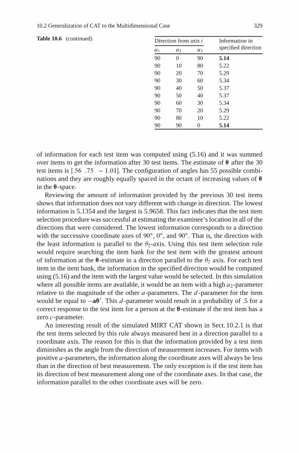
10.2 Generalization of CAT to the Multidimensional Case 329
Table 10.6 (continued) Direction from axis i Information inspecified direction˛1 ˛2 ˛3
90 0 90 5.1490 10 80 5.2290 20 70 5.2990 30 60 5.3490 40 50 5.3790 50 40 5.3790 60 30 5.3490 70 20 5.2990 80 10 5.2290 90 0 5.14
of information for each test item was computed using (5.16) and it was summedover items to get the information after 30 test items. The estimate of ™ after the 30test items is Œ:56 :75 � 1:01. The configuration of angles has 55 possible combi-nations and they are roughly equally spaced in the octant of increasing values of ™
in the ™-space.Reviewing the amount of information provided by the previous 30 test items
shows that information does not vary different with change in direction. The lowestinformation is 5.1354 and the largest is 5.9658. This fact indicates that the test itemselection procedure was successful at estimating the examinee’s location in all of thedirections that were considered. The lowest information corresponds to a directionwith the successive coordinate axes of 90ı, 0ı, and 90ı. That is, the direction withthe least information is parallel to the �2-axis. Using this test item selection rulewould require searching the item bank for the test item with the greatest amountof information at the ™-estimate in a direction parallel to the �2 axis. For each testitem in the item bank, the information in the specified direction would be computedusing (5.16) and the item with the largest value would be selected. In this simulationwhere all possible items are available, it would be an item with a high a2-parameterrelative to the magnitude of the other a-parameters. The d -parameter for the itemwould be equal to �a™0. This d -parameter would result in a probability of .5 for acorrect response to the test item for a person at the ™-estimate if the test item has azero c-parameter.
An interesting result of the simulated MIRT CAT shown in Sect. 10.2.1 is thatthe test items selected by this rule always measured best in a direction parallel to acoordinate axis. The reason for this is that the information provided by a test itemdiminishes as the angle from the direction of measurement increases. For items withpositive a-parameters, the information along the coordinate axes will always be lessthan in the direction of best measurement. The only exception is if the test item hasits direction of best measurement along one of the coordinate axes. In that case, theinformation parallel to the other coordinate axes will be zero.

330 10 Computerized Adaptive Testing Using MIRT
10.2.2.2 Maximize the Determinant of the Fisher Information Matrix
Segall (1996) suggested a method for selecting the next item in a CAT that is basedon properties of the maximum likelihood estimator of ™. He notes that conditionaldistribution of ™-estimates given the true value of ™ is asymptotically multivariatenormal with variance–covariance matrix related to the Fisher information matrixgiven by
Iij
™; O™
�D �E
�@2 ln L
@�i@�j
�; (10.4)
where ™ is the true location of the examinee, O™ is the maximum likelihood estimateof location, �i and �j are the i th and j th elements of the ™-vector, and L is thelikelihood function for the set of responses up to that point in the MIRT CAT.
Specifically, the variance–covariance matrix for the estimate after the kth testitem in the adaptive test, ˙k , is approximated by the inverse of the informationmatrix,
˙k DnI™; O™k
�o�1; (10.5)
where O™k is the estimate of the location of the examinee after k test items.When estimating locations in the ™-space using MIRT models, the information
matrix is given by
Iii
™; O™k
�D
kX
`D1
h@P`.™/
@�i
i2
P` .™/Q` .™/; (10.6)
for the diagonal elements of the matrix, and
Iij
™; O™k
�D
kX
`D1
@P`.™/
@�i
@P`.™/
@�j
P` .™/Q` .™/; (10.7)
for the off diagonal elements. All of the symbols are used as previously defined.The terms within the summations are the terms in the information matrix for singletest items. The test information matrix for the estimates of ™ is the sum of the infor-mation matrices for the single items. It is also interesting to note that the diagonalelements of the information matrix are the same as the unidimensional informationfunctions along a single axis of the coordinate system.
The test item selection criterion suggested by Segall (1996) is based on a rela-tionship between the Fisher information matrix and the confidence region around theestimates of ™ specified by Anderson (1984). Anderson showed that the equivalentof a confidence interval around the estimate of ™ is an ellipsoid in the multivariatespace. The volume of this ellipsoid is a function of ˙k . Segall (1996) showed thatwhen the following expression is maximized, the volume of the confidence ellipsoidaround the ™-estimate is minimized.
ˇˇI™; O™k
�C I .™; ukC1/
ˇˇ : (10.8)
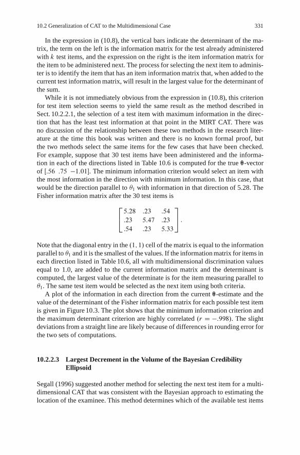
10.2 Generalization of CAT to the Multidimensional Case 331
In the expression in (10.8), the vertical bars indicate the determinant of the ma-trix, the term on the left is the information matrix for the test already administeredwith k test items, and the expression on the right is the item information matrix forthe item to be administered next. The process for selecting the next item to adminis-ter is to identify the item that has an item information matrix that, when added to thecurrent test information matrix, will result in the largest value for the determinant ofthe sum.
While it is not immediately obvious from the expression in (10.8), this criterionfor test item selection seems to yield the same result as the method described inSect. 10.2.2.1, the selection of a test item with maximum information in the direc-tion that has the least test information at that point in the MIRT CAT. There wasno discussion of the relationship between these two methods in the research liter-ature at the time this book was written and there is no known formal proof, butthe two methods select the same items for the few cases that have been checked.For example, suppose that 30 test items have been administered and the informa-tion in each of the directions listed in Table 10.6 is computed for the true ™-vectorof Œ:56 :75 �1:01. The minimum information criterion would select an item withthe most information in the direction with minimum information. In this case, thatwould be the direction parallel to �1 with information in that direction of 5.28. TheFisher information matrix after the 30 test items is
2
45:28 :23 :54
:23 5:47 :23
:54 :23 5:33
3
5 :
Note that the diagonal entry in the .1; 1/ cell of the matrix is equal to the informationparallel to �1 and it is the smallest of the values. If the information matrix for items ineach direction listed in Table 10.6, all with multidimensional discrimination valuesequal to 1.0, are added to the current information matrix and the determinant iscomputed, the largest value of the determinate is for the item measuring parallel to�1. The same test item would be selected as the next item using both criteria.
A plot of the information in each direction from the current ™-estimate and thevalue of the determinant of the Fisher information matrix for each possible test itemis given in Figure 10.3. The plot shows that the minimum information criterion andthe maximum determinant criterion are highly correlated .r D �:998/. The slightdeviations from a straight line are likely because of differences in rounding error forthe two sets of computations.
10.2.2.3 Largest Decrement in the Volume of the Bayesian CredibilityEllipsoid
Segall (1996) suggested another method for selecting the next test item for a multi-dimensional CAT that was consistent with the Bayesian approach to estimating thelocation of the examinee. This method determines which of the available test items

332 10 Computerized Adaptive Testing Using MIRT
169.5 170 170.5 171 171.5 172 172.5 1735.2
5.3
5.4
5.5
5.6
5.7
5.8
5.9
6
6.1
6.2
Determinant of Fisher Information Matrix
Info
rmat
ion
in E
ach
Direc
tion
Fig. 10.3 Plot of test information in each direction and determinant of the Fisher informationcriteria for items selected to measure in each direction at Œ1:74 �:32 �1:75
will result in the largest decrease in the volume of the Bayesian credibility ellipsoidfor the estimate of the location of the person. This method assumes that there isprior information about the distribution of coordinates for the examinee populationand that the variance–covariance matrix for this prior distribution can be specifiedin advance. Segall (1996) assumed that the prior distribution for the ™-coordinateswas multivariate normal with variance–covariance matrix ˆ. He then showed thatthe volume of the Bayesian credibility ellipsoid for the estimate of ™ is related to thefollowing expression:
ˇˇˇI™; O™k
�C I .™; ukC1/C ˆ�1
ˇˇˇ : (10.9)
When this expression is maximized, the volume of the credibility ellipsoid is min-imized. The expression in (10.9) differs from that in (10.8) by the addition of theinverse of the prior variance–covariance matrix term. If the variance–covariancematrix is the identity matrix, it will have no effect on the test item selection process.
To show the influence of the prior distribution on the test item selection process,an adaptive test in three dimensions was simulated using prior variance–covariancematrices of
C1 D2
41 :5 :5
:5 1 :5
:5 :5 1
3
5 and C2 D2
41 :9 :55
:9 1 :15
:55 :15 1
3
5 :

10.2 Generalization of CAT to the Multidimensional Case 333
Table 10.7 The item parameters for the first 15 items of a Bayesian CAT using two different priorvariance–covariance matrices
Item number C1 C2
a1 a2 a3 d a1 a2 a3 d
1 :58 :58 :58 0 .58 :58 :58 0
2 :64 :50 :58 �:43 .64 :77 :00 �:523 :17 :87 :47 �:12 .50 :17 :85 �:404 1:00 0 0 �:01 .64 :77 :00 �:875 0 0 1:00 :08 .34 0 :94 �:676 0 1:00 0 :16 .64 :77 :00 �1:137 1:00 0 0 �:32 .64 :77 :00 �1:198 0 0 1:00 :40 .34 0 :94 �:229 0 1:00 0 �:09 .17 0 :98 �:8410 1:00 0 0 �:56 .64 :77 :00 �:8211 0 0 1:00 :18 .17 0 :98 �:9012 0 1:00 0 �:30 .17 0 :98 �:8813 :98 0 :17 �:78 .64 :77 :00 �:8714 0 0 1:00 �:05 .17 0 :98 �:9315 :50 :87 0 �:51 .64 :77 :00 �:92Estimate of ™ 1:47 :83 �:60 .85 1:61 �1:89
The first variance–covariance matrix is relatively uninformative in that the corre-lations between the coordinates are all of moderate size and they are equal. Thesecond variance–covariance matrix is fairly extreme with high and low correlations.Table 10.7 shows the item parameters for the selected test items for the first 15 testitems for the two different priors for the same true ™-vector of Œ1:6 :8 �1:1. Thelast line of the table shows the estimated ™-vector for each case after a 60-item CATusing Bayesian estimation and item selection.
The results in Table 10.7 show the effect of the selection of the prior distributionon the item selection and ™-estimation. For the C1-case, except for the first few testitems, the test items selected follow the same pattern as for the procedures describedin Sect. 10.2.2.1 and 10.2.2.2. That is, the test items selected tend to alternate beingmost sensitive to differences parallel to each of the coordinate axes. For the C2-case,however, the test items are selected to measure best for a composite of the highlycorrelated dimensions. For this example, the highest correlation is between �1 and�2. Occasionally, a test item is selected to be sensitive to differences mainly along �3.
The estimation of ™ is also different for the two different selections of prior dis-tributions. The C1-case gives ™-estimates that have the correct order of magnitude,although the �3-estimate is quite different from the value used to generate the re-sponses to the test items. Case C2 yields quite a different result for the estimatesof ™. The estimates for all three dimensions show large differences from the val-ues used to generate the responses. These results are likely a function of the largedifference in correlations used in the prior multivariate distribution. While thesecorrelations are quite different and the correlations are relatively large, they are con-sistent with the correlations in the example given by Segall (1996). The results from

334 10 Computerized Adaptive Testing Using MIRT
the example suggest that using a prior distribution with large correlations may re-sult in inaccurate estimates of ™. Little research is present in the literature about thefunctioning of these item selection and estimation methods. More evaluative workneeds to be done on these methods before they can be used with confidence.
10.2.2.4 Maximize Kullback–Leibler Information
Another approach to selecting test items for a multidimensional CAT was proposedby Veldkamp and van der Linden (2002). This method uses a different measureof the sensitivity of test items to differences in persons’ locations in the ™-spacecalled Kullback–Leibler information (Kullback 1968). This approach was proposedby Chang and Ying (1996) for a unidimensional CAT to solve the problem of iden-tifying appropriate test items when estimates of � were poor early in the CAT.Lehmann and Casella (1998, p. 259) indicate that this information statistic indi-cates the amount of information for discriminating between two density functions.For this application, the likelihood functions for two possible ™-locations are usedas the density functions.
Suppose that the true location of an examinee is indicated by ™0 and that there isanother possible location denoted by ™. Then, for item response ui to a test item, theKullback–Leibler information is given by
Ki.™; ™0/ D E
�lnL.™0jui /L.™jui /
�; (10.10)
where ln is the natural logarithm and the likelihood function L is defined as
L.™jui / D Pi .™/uiQi.™/
.1�ui /: (10.11)
When only one test item is considered, the Kullback–Liebler information isgiven by
Ki.™; ™0/ D Pi.™0/ ln
�Pi.™0/
Pi .™/
�C Œ1 � Pi.™0/ ln
�Qi.™0/
Qi.™/
�: (10.12)
For the case when the probability of correct response at ™0 is .5 and the probabilityof correct response at ™ is .7, K D :087. As the likelihoods become more different,the value forK increases. For example, if the probability of a correct response to theitem at ™ is .9, then K D :51. Veldkamp and van der Linden (2002) show that theKullback–Liebler information for n items is equal to the sum of the information forthe individual items if the assumption of local independence holds,
Kn .™; ™0/ DnX
iD1Ki .™; ™0/: (10.13)
10.2 Generalization of CAT to the Multidimensional Case 335
The item selection rule suggested by Veldkamp and van der Linden is to selectthe item that maximizes the posterior expected Kullback–Leibler information. Thisis the information weighted by the posterior density function for the ™ estimate. Theexpression for the expected information is given by
KBi
O™k�1� DZ
™
Ki
™; O™k�1�
f .™ju1; � � � ; uk�1/@™; (10.14)
where KBi is the Bayesian posterior expected information, O™k�1
is the estimate oflocation after k � 1 test items, and f .™ju1; � � � ; uk�1/ is the posterior density afterk � 1 items.
Veldkamp and van der Linden (2002) used Gauss–Hermite quadrature to evaluatethe integral in (10.14), but other quadrature methods can be used as well. The keyfeature of this method is that early in the MIRT CAT test items are selected that aregood at differentiating the current estimate of ™ from other possible ™-vectors overa significant portion of the ™-space. As the estimates of ™ improve, the selection ofthe test items becomes more focused.
The implementation of the item selection based on the Kullback–Leibler infor-mation is somewhat complex because it requires the evaluation of two integrals, onefor estimating the posterior density function for the ™-estimate given the responsestring and the item parameters, and the second for evaluating the expectation givenin (10.14). My own attempts at implementing this item selection methodology inthree dimensions was very computationally slow using the triple integral quadratureprocedure from MATLAB. For that reason, no examples of the item selection re-sults are provided here. This should not be taken as a strong negative factor for thismethod because it is likely that more efficient programming methods are possible.However, as the number of dimensions for the ™-space increases, the evaluation ofthe integrals will no doubt increase the computer processing time. With fast com-puters and efficient programming, that may not be a problem.
10.2.3 Stopping Rules
The stopping rules for a CAT fall into two general categories – fixed length and vari-able length. The fixed length stopping rule is very simple. The total number of testitems to be administered to an examinee is determined in advance of implement-ing the testing procedure, and when that number of test items is reached, the finalability estimate is computed. The number of test items selected for the fixed lengthstopping rule might be based on practical considerations of testing time, or on anevaluation of the desired size for the error ellipse or posterior credibility region forthe test. Another alternative is to determine the desired accuracy for a decision to bemade for the test. The average test length needed for that decision accuracy couldbe selected as the fixed test length. The research studies referenced in this chapterused fixed length multidimensional adaptive tests.

336 10 Computerized Adaptive Testing Using MIRT
Variable length adaptive tests select a statistical criterion to control the length ofthe test. For example, a specified volume of the posterior credibility ellipsoid couldbe used to determine when to stop the test. After each test item is administered, thevolume of the credibility ellipsoid is computed, and if it is less than the specifiedvolume, the test is terminated and a final estimate of the examinees location is com-puted. Information or decision criteria could also be used for determining when tostop administering test items. As the label suggests, variable length adaptive testsadminister different numbers of test items to different examinees. The number willdepend on where the examinee is located in the ™-space, the consistency of the ex-aminee’s responses to the test items, and the amount of information provided by theitem pool in the region near the examinee’s location. Little research was found inthe literature on the features of variable length multidimensional CATs. This is animportant area for future research.
10.2.4 Item Pool
CATs are very sophisticated methodological procedures with substantial theoreticalunderpinnings. It is clear from the work that has been done so far that CATs workwell and that MIRT-CATs have strong potential. However, the best of the CAT pro-cedures will not work well if the items available for selection are not appropriate forthe examinees in the examinee population. Therefore, the design and developmentof the item pool for a CAT is critical for its proper functioning.
No research could be found that specifically addressed the design of item poolsfor MIRT-CAT procedures. Those studies of MIRT-CAT that do appear in the re-search literature use either simulated item pools or real item pools created fromexisting paper-and-pencil tests. For example, Veldkamp and van der Linden (2002)used a 176-item pool from the paper-and-pencil ACT Assessment Program. Lee, Ipand Fuh (2008) used a 480-item simulated item pool with items divided into fourlevels of discrimination. The results of these studies are dependent on the quality ofthe item pool that is used.
In earlier sections of this chapter, demonstrations were presented of MIRT-CATsusing a variety of ™-estimation and item selection procedures. For these demonstra-tions, all items were assumed to have multidimensional discrimination values of 1.0and the directions of best measurement and the multidimensional difficulty weredetermined to optimize the selection criterion. Ideal item sets were identified for theexamples. The item sets shown in Tables 10.1 and 10.3 suggest that an optimal itempool for an MIRT-CAT would have an equal number of test items with directionsof best measurement parallel to the coordinate axes, and a roughly uniform distri-bution of multidimensional difficulty over the range of ™s that is of interest. Realitem pools are not likely to meet these strict requirements. A good target for an itempool would be items with directions of best measurement that are within 15ı of thecoordinate axes and a good spread of difficulty along each axis.

10.3 Future Directions for MIRT-CAT 337
When there is a strong Bayesian prior with relatively high covariances, the itempool needs different specifications. The C2-case in Table 10.7 shows that manyof the items that were selected had directions of best measurement that were forcombinations of �s. An ideal pool for this case would require items that measuredcomposites of �s rather than measuring parallel to the coordinate axes. There wouldalso need to be a spread of difficulties so that the range of ™-vectors in the populationof examinees would be accurately estimated.
The lack of work on item pool design for MIRT-CAT shows that this is anarea that is ripe for future research. Questions such as “How large an item pool isneeded?” and “How does the size of the needed item pool change with the numberof dimensions?” need to be addressed.
10.3 Future Directions for MIRT-CAT
Although development of MIRT began many years ago, practical applications of themethodology are fairly recent. MIRT-CAT is even younger as an area of researchand application so practical applications are likely years in the future. However,progress is being made on practical issues for MIRT-CAT. Lee, Ip and Fuh (2008)investigated exposure control for MIRT-CAT using the a-stratified methodology.Veldkamp and van der Linden (2002) considered content balancing within theMIRT-CAT framework using the shadow test approach. It is likely that much moreresearch will be done on MIRT-CAT with the goal of bringing this methodology tothe point that it can be used for operational testing programs.
Some obvious areas for future research are easy to identify. Most of the publishedresearch is for the special case of two-coordinate axes. It seems unrealistic to assumethat most practical applications will fit within this simple framework. Work needsto be done to determine how well methods work when three or more coordinatesare used to specify the location of individuals in the ™-space. Most of the currentresearch also uses fixed length tests. It will be useful to investigate the number ofitems needed to converge to within a specified distance from the true ™-location.This research may not lead to the implementation of variable length MIRT-CAT, butit would at least provide information on what is the appropriate length for a fixedlength CAT.
Developing guidelines for item pools for MIRT-CAT is another obvious area forfuture research. Of course, this needs to be connected to work on the practical de-velopment of test items to match the specifications for such item pools. If item poolspecifications indicated that test items are needed that measure an equally weightedcomposite of two constructs, will it be possible to construct the required test items?
MIRT-CAT is an exciting area for new development. It will be interesting towatch the research literature and presentations at professional meetings to note thedirections (probably multiple directions) that these developments take.

338 10 Computerized Adaptive Testing Using MIRT
10.4 Exercises
1. Suppose that an MIRT-CAT procedure is designed to function in a ™-space withfour coordinate axes. It was determined that the first item to be administered shouldhave a direction of best measurement that has equal angles with all of the coordi-nate axes. If the multidimensional discrimination for this item is 1.0, what is thea-parameter vector for this item and what is the angle for the item vector for thisitem with each coordinate axis?
2. The third sentence below (10.9) indicates that if the prior variance–covariancematrix is the identity matrix, then selecting a test item to minimize the volume ofthe credibility ellipsoid will give the same result as maximizing the determinant ofFisher information matrix. Explain why this is the case.
3. Consider the results given in Table 10.7. How do the second items in the testsusing the different prior distributions differ in what they best measure? Explain whydifferent items were selected when both tests had the same first item and the sameresponse from the examinee.
4. Draw a diagram that shows the processes that need to be performed in a CAT andthe connections between the processes. Clearly label each of the parts of the diagramand show the flow of the testing process with arrows connecting the processes.
5. How do the diagonal entries of the Fisher information matrix relate to unidi-mensional estimates of information? Also, how does the information in differentdirections in the ™-space relate to the Fisher information matrix?
6. In Table 10.6, which direction of measurement has the greatest amount of infor-mation at the current estimate of ™? How much does the information in the directionof most information differ from that with the least information? What does thisdifference indicate about the success or failure of the MIRT-CAT process after theadministration of 30 test items? Would it be desirable to have a larger difference inthe amount of information in the different directions from the current estimate?
7. When using maximum likelihood estimation for an MIRT-CAT, why is it appro-priate to minimize the negative log likelihood rather than maximize the likelihood?Provide an example to support your argument.
8. Compare the results after two items have been administered in Tables 10.1 and10.2. How do the items selected to be administered third in the test differ? Howdo the ™-estimates after two items have been administered differ? Explain why theestimates are different.
9. Does (10.7) indicate that the Fisher information matrix is a symmetric matrix?Explain your reasoning.

10.4 Exercises 339
10. Select a test battery that contains a number of tests. Suppose that you wouldlike to create an MIRT-CAT to estimate an examinee’s performance on all of thetests at the same time using a Bayesian estimation and test item selection method.What variance–covariance matrix would you specify for the prior distribution forthis MIRT-CAT? Explain how you arrived at this prior distribution and defend yourselection.

References
Abrahamowicz M, Ramsay JO (1992) Multicategorical spline model for item response theory.Psychometrika 57:5–27
Ackerman TA (1992) A didactic explanation of item bias, item impact, and item validity from amultidimensional perspective. Journal of Educational Measurement 29:67–91
Ackerman TA (1996) Graphical representation of multidimensional item response theory analyses.Applied Psychological Measurement 20:311–329
Ackerman TA, Gierl MJ, Walker CM (2003) Using multidimensional item response theory toevaluate educational and psychological tests. Educational Measurement: Issues and Practice22:37–51
ACT, Inc. (2007) The ACT technical manual. ACT, Inc., Iowa City, IAAdams RJ, Wilson M, Wang W (1997) The multidimensional random coefficients multinomial
logit model. Applied Psychological Measurement 21:1–24Anderson TW (1984) An introduction to multivariate statistical analysis (2nd ed.). John Wiley,
New YorkAndrich D (2004) Controversy and the Rasch model: A characteristic of incompatible paradigms?
Medical Care 42:I-7–I-16Apostle TM (1957) Mathematical analysis. Addison-Wesley, Reading, MAAsimov I (1972) Asimov’s new guide to science. Basic Books, New YorkBai J, Ng S (2002) Determining the number of factors in approximate factor models. Econometrica
70:191–221Baker FB, Kim S-H (2004) Item response theory: Parameter estimation techniques (2nd edition,
revised and expanded). Marcel Dekker, New YorkBayes, T (1793) An essay towards solving a problem in the doctoring of chances. Philosophical
Transactions of the Royal Society of London 53:370–418Beguin AA, Glas CAW (2001) MCMC estimation and some model-fit analysis of multidimensional
IRT models. Psychometrika 66:541–561Bejar II (1977) An application of the continuous response level model to personality measurement.
Applied Psychological Measurement 1:509–521Binet A, Simon T (1913) A method of measuring the development of intelligence in children
(Translated from the French by CH Town). Chicago Medical Book Company, ChicagoBirnbaum A (1968) Some latent trait models and their use in infering an examinee’s ability. In FM
Lord MR Novick (eds.) Statistical theories of mental test scores. Addison-Wesley, Reading,MA
Bloxom B Vale CD (1987) Multidimensional adaptive testing: an approximate procedure forupdating. Paper presented at the annual meeting of the Psychometric Society, Montreal
Bock RD, Aitkin M (1981) Marginal maximum likelihood estimation of item parameters: Appli-cations of an EM algorithm. Psychometrika 46:443–459
Bock RD, Gibbons R, Muraki E (1988) Full information item factor analysis. Applied Psycholog-ical Measurement 12:261–280
341
342 References
Bock RD, Schilling SG (2003) IRT based item factor analysis. In M du Toit (ed) IRT from SSI:BILOG-MG, MULTILOG, PARSCALE, TESTFACT (pp. 584–591). Scientific Software Inter-national, Lincolnwood, IL
Bolt DM, Lall VF (2003) Estimation of compensatory and noncompensatory multidimensionalitem response models using Markov chain Monte Carlo. Applied Psychological Measurement27:395–414
Bulfinch T (1855) The age of fable. Reprinted in Bulfinch’s mythology. The Modern Library,New York
Burgess MA (1921) The measurement of silent reading. Russell Sage Foundation, New YorkCamilli G (1994) Origin of the scaling constant d = 1.7 in item response theory. Journal of Educa-
tional and Behavioral Statistics 19:293–295Camilli G, Wang M, Fesq J (1995) The effects of dimensionality on equating the Law School
Admissions Test. Journal of Educational Measurement 32:79–96Carroll JB (1945) The effect of difficulty and chance success on correlations between items or
between tests. Psychometrika 10:1–19Carroll JB (1993) Human cognitive abilities: A survey of factor analytic studies. Cambridge
University Press, New YorkChang H-H, Ying Z (1996) A global information approach to computerized adaptive testing.
Applied Psychological Measurement 20:213–230Chib S, Greenberg E (1995) Understanding the Metropolis-Hastings algorithm. The American
Statistician 49:327–335Christoffersson A (1975) Factor analysis of dichotomized variables. Psychometrika 40:5–32Davey TC, Ackerman TA, Reckase MD, Spray JA (1989) Interpreting score differences when item
difficulty and discrimination are confounded. Paper presented at the meeting of the Psychome-tric Society, Los Angeles
Davey TC, Oshima TC (1994) Linking multidimensional calibrations. Paper presented at the an-nual meeting of the National Council on Measurement in Education, New Orleans
Deese J (1958) The psychology of learning (2nd edition). McGraw-Hill, New YorkDeGroot MH (1970) Optimal statistical decisions. McGraw-Hill, New YorkDempster AP, Laird NM, Rubin DB (1977) Maximum likelihood from incomplete data via the EM
algorithm (with discussion). Journal of the Royal Statistical Society Series B 39:1–38Dorans NJ, Pommerich M, Holland PW (eds) (2007) Linking and aligning scores and scales.
Springer, New YorkDrasgow F, Parsons CK (1983) Applications of unidimensional item response theory to multidi-
mensional data. Applied Psychological Measurement 7:189–199Ebbinghaus H (1885) Uber das Gedachtnis: Untersuchungen zur experimentalen Psychologie.
Duncker and Humbolt, LeipzigEmbretson SE (1991) A multidimensional latent trait model for measuring learning and change.
Psychometrika 56:495–515Fischer GH (1995a) Derivations of the Rasch model. In Fischer GH and Molenaar IW (eds) Rasch
models: Foundations, recent developments and applications. Springer-Verlag, New YorkFischer GH (1995b) Linear logistic test models for change. In Fischer GH and Molenaar IW (eds)
Rasch models: Foundations, recent developments and applications. Springer-Verlag, New YorkFischer GH, Molenaar IW (eds) (1995) Rasch models: Foundations, recent developments, and
applications. Springer-Verlag, New YorkFisher RA (1925) Theory of statistical estimation. Proceedings of the Cambridge Philosophical
Society 22:700–725Fraser C (1998) NOHARM: A Fortran program for fitting unidimensional and multidimensional
normal ogive models in latent trait theory. The University of New England, Center for Behav-ioral Studies, Armidale, Australia
Frederiksen N, Glaser R, Lesgold A, Shafto MG (eds) Diagnostic monitoring of skill and knowl-edge acquisition. Lawrence Erlbaum Associates, Hillsdale, NJ
Galton F (1870) Hereditary genius: An inquiry into its laws and consequences. D. Appleton,London

References 343
Gamerman D, Lopes HF (2006) Markov chain Monte Carlo: Stochastic simulation for Bayesianinference (2nd edition). Chapman & Hall, Boca Raton, FL
Geman S, Geman D (1984) Stochastic relaxation, Gibbs distributions, and the Bayesian restorationof images. IEEE Transactions on Pattern Analysis and Machine Intelligence 6:721–741
Gentle JE (1998) Numerical linear algebra for applications in statistics. Springer, New YorkGessaroli ME, De Champlain AF (1996) Using an approximate chi-square statistic to test the
number of dimensions underlying the responses to a set of items. Journal of Educational Mea-surement 33:157–179
Glas CAW (1992) A Rasch model with a multivariate distribution of ability. In Wilson M (ed)Objective measurement: Theory into practice volume 1. Ablex, Norwood, NJ
Glas CAW, Vos HJ (2000) Adaptive mastery testing using a multidimensional IRT model andBayesian sequential decision theory (Research Report 00-06). University of Twente, Enschede,The Netherlands
Gosz JK, Walker CM (2002) An empirical comparison of multidimensional item response theorydata using TESTFACT and NOHARM. Paper presented at the annual meeting of the NationalCouncil for Measurement in Education, New Orleans
Gower JC, Dijksterhuis GB (2004) Procrustes problems. Oxford University Press, Oxford, EnglandGulliksen H (1950) Theory of mental tests. Wiley, New YorkHaberman SJ (1977) Log-linear models and frequency tables with small expected cell counts.
Annals of Statistics 5:1148–1169Haebara T (1980) Equating logistic ability scales by a weighted least squares method. Japanese
Psychological Research 22:144–149Haley DC (1952) Estimation of the dosage mortality relationship when the dose is subject to error
(Technical Report No. 15). Stanford University Applied Mathematics and Statistics Laboratory,Stanford, CA
Hambleton R, Swaminathan H (1983) Item response theory: principles and applications. Kluwer,Boston
Harman HH (1976) Modern factor analysis (3rd edition revised). The University of Chicago Press,Chicago
Hastings WK (1970) Monte Carlo simulation methods using Markov chains and their applications.Biometrika 57:97–109
Healy AF, McNamara DS (1996) Verbal learning and memory: Does the modal model still work?In Spence JT, Darley JM, Foss DJ (eds) Annual Review of Psychology 47:143–172
Holland PW (2007) A framework and history for score linking. In Dorans NJ, Pommerich M,Holland PW (eds) Linking and aligning scores and scales. Springer, New York
Holzinger KJ, Harman HH (1941) Factor analysis: A synthesis of factorial methods. The Universityof Chicago Press, Chicago
Horn JL (1965) A rationale and test for the number of factors in factor analysis. Psychometrika32:179–185
Horst P (1965) Factor analysis of data matrices. Holt, Rinehart & Winston, New YorkHulin CL, Drasgow F, Parsons CK (1983) Item response theory: application to psychological mea-
surement. Dow Jones-Irwin, Homewood, ILJang EE, Roussos L (2007) An investigation into the dimensionality of TOEFL using conditional
covariance-based nonparametric approach. Journal of Educational Measurement 44:1–21Kallon AA (1916) Standards in silent reading. Boston Department of Educational Investigation
and Measurement Bulletin No. 12, School Document 18. BostonKelderman H (1994) Objective measurement with multidimensional polytomous latent trait mod-
els. In Wilson M (ed) Objective measurement: Theory into practice, Vol. 2. Ablex, NorwoodNJ
Kelderman H, Rijkes CPM (1994) Loglinear multidimensional IRT models for polytomouslyscored items. Psychometrika 59:149–176
Kendall MG, Stuart A (1961) The advanced theory of statistics. Hafner, New YorkKim HR (1994) New techniques for the dimensionality assessment of standardized test data. Un-
published doctoral dissertation, University of Illinois, Champaign-Urbana, IL

344 References
Kim J-P (2001) Proximity measures and cluster analyses in multidimensional item response theory.Unpublished doctoral dissertation, Michigan State University, East Lansing, MI
Kirisci L, Hsu T, Yu L (2001) Robustness of item parameter estimation programs to assumptionsof unidimensionality and normality. Applied Psychological Measurement 25:146–162
Kolen MJ, Brennan RL (2004) Test equating, scaling, and linking: Methods and practices (2ndedition) Springer, New York
Kulback S (1968) Information theory and statistics (2nd edition). Dover, New YorkLedesma RD, Valero-Mora P (2007) Determining the number of factors to retain in EFA: an easy-
to-use computer program for carrying out parallel analysis. Practical Assessment, Research &Evaluation 12:1–11
Lehmann EL, Casella G (1998) Theory of point estimation (2nd edition). Springer-Verlag,New York
Lee Y-H, Ip EH, Fuh C-D (2008) A strategy for controlling item exposure in multidimensionalcomputerized adaptive testing. Educational and Psychological Measurement 68:215–232
Lord FM (1980) Applications of item response theory to practical testing problems. LawrenceErlbaum Associates, Hillsdale, NJ
Lord FM, Novick MR (1968) Statistical theories of mental test scores. Addison-Wesley, Reading,MA
MacCorquidale K, Meehl PE (1948) On a distinction between hypothetical constructs and inter-vening variables. Psychological Review 55:95–107
Maris E (1995) Psychometric latent response models. Psychometrika 60:523–547Masters GN (1982) A Rasch model for partial credit scoring. Psychometrika 47:149–174Masters GN, Wright BD (1997) The partial credit model. In WJ van der Linden RK Hambleton
(eds.) Handbook of modern item response theory. Springer, New YorkMaydeu-Olivares A (2001) Multidimensional item response theory modeling of binary data: Large
sample properties of NOHARM estimates. Journal of Educational and Behavioral Statistics26:51–71
McCall WA (1922) How to measure in education. The Macmillan Company, New YorkMcDonald RP (1967) Nonlinear factor analysis. Psychometric Monograph 15McDonald RP (1985) Factor analysis and related methods. Lawrence Erlbaum Associates, Hills-
dale, NJMcDonald RP (1997) Normal-ogive multidimensional model. In WJ van der Linden and
RK Hambleton (eds) Handbook of modern item response theory. Springer, New YorkMcDonald RP (1999) Test theory: A unified treatment. Lawrence Erlbaum Associates, Mahwah,
NJMcKinley RL, Reckase MD (1982) The use of the general Rasch model with multidimensional
item response data (Research Report ONR 82-1). American College Testing, Iowa City, IAMetropolis N, Rosenbluth AW, Rosenbluth MN, Teller AH, Teller E (1953) Equations of state
space calculations by fast computing machines. Journal of Chemical Physics 21:1087–1091Miller MD, Linn RL (1988) Invariance of item characteristic functions with variations in instruc-
tional coverage. Journal of Educational Measurement 25:205–219Miller TR (1991) Empirical estimation of standard errors of compensatory MIRT model parameters
obtained from the NOHARM estimation program (Research Report ONR 91-2). AmericanCollege Testing Program, Iowa City, IA
Miller TR, Hirsch TM (1992) Cluster analysis of angular data in applications of multidimensionalitem response theory. Applied Measurement in Education 5:193–211
Millman J, Greene J (1989) The specification and development of tests of achievement and ability.In Linn RL (ed) Educational measurement (3rd edition). American Council on Education andMacmillan, New York
Moulton MH (2004) One use of a non-unidimensional scaling (NOUS) model: Transferring infor-mation across dimensions and subscales. Educational Data Systems, Morgan Hill, CA
Mroch AA, Bolt DM (2006) A simulation comparison of parametric and nonparametric dimen-sionality detection procedures. Applied Measurement in Education 19:67–91

References 345
Mulaik SA (1972) A mathematical investigation of some multidimensional Rasch models for psy-chological tests. Paper presented at the annual meeting of the Psychometric Society, Princeton,NJ
Muraki E, Carlson JE (1993) Full-information factor analysis for polytomous item responses. Paperpresented at the annual meeting of the American Educational Research Association, Atlanta
Muraki E, Englelhard G Jr (1985) Full-information item factor analysis: applications of EAPscores. Applied Psychological Measurement 9:417–430
Muthen B (1978) Contributions to factor analysis of dichotomous variables. Psychometrika43:551–560
Oshima TC, Davey TC, Lee K (2000) Multidimensional linking: Four practical approaches. Journalof Educational Measurement 37:357–373
Osterland SJ (1990) Toward a uniform definition of a test item. Educational Research Quarterly14:2–5
Owen RJ (1975) A Bayesian sequential procedure for quantal response in the context of adaptivemental testing. Journal of the American Statistical Association, 70:351–356
Parshall CG, Spray JA, Davey T (2002) Practical considerations in computer-based testing.Springer, New York
Patz RJ, Junker BW (1999) A straightforward approach to Markov chain Monte Carlo methods foritem response models. Journal of Educational and Behavioral Statistics 24:146–178
Perie M, Grigg W, Donahue P (2005) The Nation’s Report Card: Reading 2005 (NCES 2006-451). U.S. Department of Education, National Center for Education Statistics, U.S. GovernmentPrinting Office, Washington, DC
Rasch G (1960) Probabilistic models for some intelligence and attainment tests. Danmarks Paeda-gogiske Institut, Copenhagen
Rasch G (1962) On general laws and the meaning of measurement in psychology. Proceedings ofthe fourth Berkeley symposium on mathematical statistics and probability 4:321–334
Reckase MD (1972) Development and application of a multivariate logistic latent trait model.Unpublished doctoral dissertation, Syracuse University, Syracuse, NY
Reckase MD (1985) The difficulty of test items that measure more than one ability. Applied Psy-chological Measurement 9:401–412
Reckase MD, Ackerman TA, Carlson JE (1988) Building a unidimensional test using multidimen-sional items. Journal of Educational Measurement 25:193–204
Reckase MD, Davey TC, Ackerman TA (1989) Similarity of the multidimensional space definedby parallel forms of a mathematics test. Paper presented at the meeting of the American Edu-cational Research Association, San Francisco
Reckase MD, Hirsch TM (1991) Interpretation of number-correct scores when the true numbers ofdimensions assessed by a test is greater than two. Paper presented at the annual meeting of theNational Council on Measurement in Education, Chicago
Reckase MD, McKinley RL (1991) The discriminating power of items that measure more than onedimension. Applied Psychological Measurement 15:361–373
Reckase MD, Stout W (1995) Conditions under which items that assess multiple abilities will be fitby unidimensional IRT models. Paper presented at the European meeting of the PsychometricSociety, Leiden, The Netherlands
Reise SP, Waller NG, Comrey AL (2000) Factor analysis and scale revision. Psychological Assess-ment 12:287–297
Rijmen F, De Boeck P (2005) A relationship between a between-item multidimensional IRT modeland the mixture Rasch model. Psychometrika 70:481–496
Roberts JS, Donoghue JR, Laughlin JE (2000) A general item response theory model for unfoldingunidimensional polytomous responses. Applied Psychological Measurement 24:3–32
Rosenbaum PR (1984) Testing the conditional independence and monotonicity assumptions ofitem response theory. Psychometrika 49:425–435
Roussos LA, Ozbek OY (2006) Formulation of the DETECT population parameter and evaluationof DETECT estimation bias. Journal of Educational Measurement 43:215–243

346 References
Roussos LA, Stout WF, Marden JL (1998) Using new proximity measures with hierarchical clusteranalysis to detect multidimensionality. Journal of Educational Measurement 35:1–30
Samejima F (1969) Estimation of latent ability using a response pattern of graded scores. Psycho-metric Monograph Supplement, 34 (Monograph No. 17)
Samejima F (1974) Normal ogive model on the continuous response level in the multidimensionalspace. Psychometrika 39:111–121
Samejima F, Livingston P (1979) Method of moments as the least squares solution for fitting apolynomial (Research Report 79-2). Univerrsity of Tennessee, Knoxville, TN
Sands WA, Waters BK, McBride JR (eds.) (1997) Computerized adaptive testing: from inquiry tooperation. American Psychological Association, Washington, DC
Savalei V (2006) Logistic approximation to the normal: the KL rationale. Psychometrika 71:763–767
Schilling S, Bock RD (2005) High-dimensional maximum marginal likelihood item factor analysisby adaptive quadrature. Psychometrika 70:533–555
Segall DO (1996) Multidimensional adaptive testing. Psychometrika 61:331–354Sinharay S, Holland PW (2007) Is it necessary to make anchor tests mini-versions of the tests being
equated or can some restrictions be relaxed? Journal of Educational Measurement 44:249–275Sokal RR, Michener CD (1958) A statistical method for evaluating systematic relationships. Uni-
versity of Kansas Science Bulletin 38:1409–1438Spiegelhalter D, Thomas A, Best N (2000) WinBUGS version 1.3 (Computer program). MRC
Biostatistics Unit, Institute of Public Health, Cambridge, EnglandSpray JA, Davey TC, Reckase MD, Ackerman TA, Carlson JE (1990) Comparison of two logis-
tic multidimensional item response theory models (Research Report ONR90-8). ACT, Inc.,Iowa City, IA
Stern W (1914) The psychological methods of testing intelligence. Warwick & York, BaltimoreStevens SS (1946) On the theory of scales of measurement. Science 103:677–680Stevens SS (1951) Mathematics, measurement, and psychophysics. In SS Stevens (ed) Handbook
of experimental psychology (pp. 1–49). Wiley, New YorkStigler SM (1986) The history of statistics: The measurement of uncertainty before 1900. Belknap
Press, Cambridge, MAStocking LM, Lord FM (1983) Developing a common metric in item response theory. Applied
Psychological Measurement 7:201–210Stone CA, Yeh C-C (2006) Assessing the dimensionality and factor structure of multiple-choice ex-
ams: An empirical comparison of methods using the Multistate Bar Examination. Educationaland Psychological Measurement 66:193–214
Stout W (1987) A nonparametric approach for assessing latent trait dimensionality. Psychometrika52:589–617
Stout W, Douglas B, Junker B, Roussos L (1999) DIMTEST [Computer software]. The WilliamStout Institute for Measurement, Champaign, IL
Stout W, Froelich AG, Gao F (2001) Using resampling to produce and improved DIMTEST pro-cedure. In Boomsma A, van Duijn MAJ, Snijders TAB (eds.) Essays on item response theory(pp. 357–375). Springer-Verlag, New York
Sympson JB (1978) A model for testing with multidimensional items. In Weiss DJ (ed) Proceedingsof the 1977 Computerized Adaptive Testing Conference, University of Minnesota, Minneapolis
Tam SS (1992) A comparison of methods for adaptive estimation of a multidimensional trait. Ph.D.thesis, Columbia University
Tate R (2003) A comparison of selected empirical methods for assessing the structure of responsesto test items. Applied Psychological Measurement 27:159–203
Thissen D, Wainer H (2001) Test scoring. Lawrence Erlbaum Associates, Mahwah, NJThorndike EL (1904) An introduction to the theory of mental and social measurements. The Sci-
ence Press, New YorkThurstone LL (1947) Multiple-factor analysis: A development and expansion of The Vectors of
Mind. The University of Chicago Press, Chicago

References 347
Timm NH (1975) Multivariate analysis with applications in education and psychology. Brooks/Cole, Monterey, CA
van der Ark LA (2001) Relationships and properties of polytomous item response theory models.Applied Psychological Measurement 25:273–282
van der Linden WJ (2005) Linear models of optimal test design. Springer, New Yorkvan der Linden WJ, Glas CAW (eds) (2000) Computerized adaptive testing: theory and practice.
Kluwer Academic, Dordrecht, The Netherlandsvan der Linden WJ, Hambleton RK (eds.) (1997) Handbook of modern item response theory.
Springer, New YorkVeldkamp BP, van der Linden WJ (2002) Multidimensional adaptive testing with constraints on
test content. Psychometrika 67:575–588Vernon P (1950) The structure of human abilities. Methuen, LondonVerhelst ND, Verstralen HHFM (1997) Modeling sums of binary responses by the partial credit
model (Measurement and Research Department Reports 97-7). Cito, Arnhem, The NetherlandsVolodin N, Adams RJ (2002) The estimation of polytomous item response models with many
dimensions. Unpublished report, University of Melbourne, Victoria, AustraliaWainer DJ, Dorans DJ, Flaugher R, Green BF, Mislevy L, Steinberg L, Thissen D (1990) Comput-
erized adaptive testing: A primer. Lawrence Erlbaum Associates, Hillsdale, NJWang M (1985) Fitting a unidimensional model to multidimensional item response data: The effect
of latent space misspecification on the application of IRT (Research Report MW: 6-24-85).University of Iowa, Iowa City, IA
Wang M (1986) Fitting a unidimensional model to multidimensional item response data. Paperpresented at the Office of Naval Research Contractors Meeting, Gatlinburg, TN
Wang W-C, Chen P-H (2004) Implementation and measurement efficiency of multidimensionalcomputerized adaptive testing. Applied Psychological Measurement 28:295–316
Wang W, Wilson M (2005) Exploring local item dependence using a random-effects facet model.Applied Psychological Measurement 29:296–318
Ward JH (1963) Hierarchical grouping to optimize an objective function. Journal of the AmericanStatistical Association 58:236–244
Warm TA (1989) Weighted likelihood estimation of ability in item response theory. Psychometrika54:427–450
Weiss DJ (1974) Strategies of adaptive ability measurement (Research Report 74-5). PsychometricMethods Program, University of Minnesota, Minneapolis
Whipple GM (1910) Manual of mental and physical tests. Warwick & York, BaltimoreWhitely SE (1980a) Measuring aptitude processes with mutlicomponent latent trait models (Tech-
nical Report No. NIE-80-5). University of Kansas, Lawrence, KSWhitely SE (1980b) Multicomponent latent trait models for ability tests. Psychometrika 45:
479–494Wilson M, Adams R (1995) Rasch models for item bundles. Psychometrika 60:181–198Wu ML, Adams RJ, Wilson MR (1997) ConQuest: Generalized item response modeling software.
ACER, Victoria, AustraliaYao L (2003) BMIRT: Bayesian multivariate item response theory. CTB/McGraw-Hill, Monterey,
CAYao L, Schwarz R (2006) A multidimensional partial credit model with associated item and
test statistics: An application to mixed-format tests. Applied Psychological Measurement 30:469–492
Yen WM (1984) Effects of local dependence on the fit and equating performance of the three-parameter logistic model. Applied Psychological Measurement 8:125–145
Yoakum CS, Yerkes RM (1920) Army mental tests. Henry Holt, New YorkZhang JM, Stout W (1999a) Conditional covariance structure of generalized compensatory multi-
dimensional items. Psychometrika 64:129–152Zhang JM, Stout W (1999b) The theoretical DETECT index of dimensionality and its application
to approximate simple structure. Psychometrika 64:213–249Zimowski MF, Muraki E, Mislevy RJ, Bock RD (2003) BILOG-MG for Windows. Scientific Soft-
ware International, Inc., Lincolnwood, IL
Index
AAckerman, T.A., 75, 124Adams, R.J., 92, 94, 100, 105, 162–165Aitken, M., 165Aitkin, M., 67, 68, 70Anderson, 330Andrich, D., 21Asimov, I., 57
BBai, J., 181Baker, F.B., 23, 138Base coordinate system, 264, 276–278, 289,
291–293, 295–300, 302, 305Base test, 263, 299Bayesian estimation, 144–146, 149, 314,
320–325, 333, 339Bayesian modal, 321–326Bejar II., 70Bias, 74, 146, 209, 210, 319, 324, 325BILOG-MG, 216Binet, A., 62Birnbaum, 21, 26, 47Biserial correlation, 21, 28–31, 81, 82Bloxom, 325, 326Bock, R.D., 67, 68, 70, 149, 151, 157, 165,
218, 219Bolt, D.M., 100, 102, 176, 182
CCalibration, 36, 71, 75, 157, 159, 161, 164,
176, 190, 193, 198, 234, 235, 239,241, 243, 244, 251, 253, 261, 262,275–278, 282, 284–286, 288, 289,291, 292, 294–296, 298–303, 308,309, 311, 313
Camilli, G., 95Carlson, J.E., 102, 107, 120
Carroll, J.B., 61Cartesian coordinate, 6, 8Casella, G., 334CAT. See Computerized adaptive testing (CAT)Category response function, 39–41, 52,
108–110Centroid plot, 131–134Chang, H.-H., 334Chen, P.-H., 325Christoffersson, A., 65Clam shell plot, 123, 130, 131Cluster analysis, 74, 220, 226–228, 278, 280,
299, 301Common factor, 31, 67, 70, 180Compensatory, 79, 80, 86–102, 104, 109, 114,
121, 126, 127, 137–139, 152, 158,171, 172, 194–196, 198, 201, 203,208, 211, 238, 244, 252, 255, 257,269, 270
Computerized adaptive testing (CAT), 275,311–337
Conditional standard error of measurement, 48Confidence interval, 47, 330Content balancing, 337Continuum, 2–5, 193Contour plot, 88, 91, 101, 113, 118, 119, 122,
127, 130, 139Coordinate
axes/axis, 6, 63, 80, 83, 86, 89, 90, 96,116, 118, 119, 121, 126, 127,134, 138, 152, 161, 173, 179, 180,183, 185, 189, 191, 193, 198, 201,202, 205, 218, 220, 221, 225, 238,239, 244–258, 260, 263, 268, 282,284–286, 291, 299, 302–304, 306,309, 315, 316, 318, 326, 333, 336
Cumulative category response function, 39, 40,52, 108
349

350 Index
DDavey, T.C., 75, 294, 295De Boeck, P., 69Dempster, A.P., 151Dichotomous items, 35, 36, 73, 85, 102, 106DIF. See Differential item functioning (DIF)Differential item functioning (DIF), 75Difficulty parameter(s), 17, 19, 22, 27, 35, 39,
40, 65, 70, 81, 89, 93, 99, 106, 113,164, 179, 243, 270, 277
Dijksterhuis, G.B., 251Dilation, 253, 256Dimension, 4, 5, 68, 69, 79, 82, 87, 89, 90, 93,
97, 104–106, 115, 127, 131, 132,140, 150, 152, 154, 157, 163–167,172–175, 180, 182, 184, 187, 189,190, 192, 201, 205, 206, 208, 215,219, 220, 226, 227, 238, 242, 243,254–256, 270, 316
DIMTEST, 12, 208–212, 214, 215, 224, 228,229
Direction cosine(s), 221, 281, 299, 306, 307Discriminating power, 2, 20, 21, 23, 31, 36, 62,
119, 157, 247, 250Discrimination, 21, 28–31, 36, 37, 39, 40, 63,
68, 71, 74, 81, 83, 86, 89, 100, 108,113–121, 123, 126, 133, 134, 152,159, 162, 183, 186, 189–192, 198,208, 221, 222, 245, 246, 249, 250,252, 255, 257, 265, 267, 268, 298,331, 336
Discrimination parameter(s), 36, 37, 39, 40,68, 73, 81, 83, 86, 89, 108, 113,118, 126, 134, 162, 164, 190, 246,249, 252, 255, 267, 268, 298
Distance formula, 5, 6, 8, 115
EEbbinghaus, H., 57Eigenvalue(s), 126, 184, 215–218, 229, 281,
300Eigenvector(s), 126, 127, 184, 215, 281, 282,
300, 303Englelhard, G. Jr., 152Equating, 71, 75, 202, 235, 243, 261, 276, 286,
287, 292, 294, 295, 298, 299, 308,309
Equi-probable contour(s), 113, 118, 119, 139,238
Expected number-correct score, 125Expected score, 29, 46, 104–107, 109, 110,
125Expected score curve, 35, 42, 43Exposure control, 313, 337
FFactor analysis, 11, 63–68, 70, 71, 74, 80, 149,
179, 180, 210, 215, 276Factor loading, 31, 65, 179Factor scores, 276Fischer, G.H., 11, 69Fisher information, 330–332Fisher, R.A., 51Fixed step size, 315, 316, 321Fraser, C., 158Fuh, C.-D., 325, 336, 337Full information factor analysis, 70
GGalton, F., 58Gamerman, D., 138General Rasch model, 69, 92Generalized partial credit model, 32, 36–38,
51, 52, 55, 102–104, 110Gessaroli, M.E., 225Gibbons, R., 68, 149, 151Glas, C.A.W., 69Gower, J.C., 251Graded response model
multidimensional, 107, 110, 120unidimensional, 107
Greene, J., 62Gulliksen, H., 62
HHaebara, T., 295Haley, D.C., 95Hambleton, R.K., 11, 32, 48Harman, H.H., 6, 63, 179, 221Hirsch, T.M., 70, 74Holland, P.W., 275, 276Holzinger, K.J., 179Horn, J.L., 215Horst, P., 65Hulin, 11Hyperplane, 238, 247Hypothetical construct, 3, 4, 29, 59, 69, 79–82,
108, 137
– 3,51 5

Index 351
IICC. See Item characteristic curve (ICC)Indeterminacy, 106, 152, 158, 160, 167, 168,
172, 175, 233–235, 239, 244, 252,257, 262, 270
InformationInformation function(s), 43, 47–53, 122,
123, 213, 330Information surface, 122, 123, 129, 130
Invariance property, 235, 242, 243, 255, 257,266–268, 270, 278, 281, 282, 298
Ip, E.H., 325, 336, 337IRT. See Item response theory (IRT)Item bank, 71, 275, 311–314, 320, 326–335Item characteristic curve (ICC), 17–27, 29, 35,
46, 97, 113, 114, 118, 277Item pool, 275, 311, 336–337Item response theory (IRT), 9, 12, 13, 17, 21,
25–27, 29, 30, 32, 43, 44, 47, 48,51–54, 59, 60, 63, 67, 68, 70, 71, 74,75, 81, 82, 102, 126, 129, 133, 134,144, 172, 184, 185, 189, 194, 196,198–200, 209, 212, 215, 233, 234,246, 270, 277, 295, 309, 311, 313
Item score string, 139, 145–150, 152, 164, 320Item statistics, 26–32Item vectors, 180, 183, 185, 186, 190, 198,
199, 201, 203, 205, 206, 221, 222,224, 235, 239, 241, 245, 256, 257,264, 278, 280–282, 284, 286, 288,291, 292, 294, 302–304
JJang, E.E., 213Junker, B.W., 165
KKelderman, H., 69, 104, 110Kendall, 47Kim, J.-P., 221Kim, S.-H., 23, 138Kullback-Leibler information, 53, 334–335
LLaird, N.M., 151Lall, V.F., 100, 102, 176Ledesma, 215, 216Lee, K., 294, 295Lee, Y.-H., 325, 336, 337Lehmann, E.L., 334Linking, 71, 75, 261, 275–309
Local independence, 9, 12–14, 50, 66, 67, 69,77, 84, 195, 199, 212, 334
log likehihood, 142, 314, 321Logistic model
three-parameter, 23–26, 44, 46, 49, 62, 81,91, 142, 269
two-parameter, 21–25, 28, 36, 38–40, 46,49, 73, 86, 89, 92, 95, 96, 108, 113,122, 123, 128, 149, 183, 185, 194,198, 235, 238, 267, 269
Lopes, H.F., 138Lord, F.M., 11, 15, 21, 44, 46–52, 68–70, 91,
295Lower asymptote, 17, 23–25, 31–32, 46, 50,
91, 96–98, 104, 269Lower asymptote parameter, 23, 27, 31, 32, 99,
142, 149, 216
MM2pl model. See Multidimensional extension
of the two-parameter logistic (M2pl)model
Maris, E., 99Martineau, J., 269Masters, 35, 36MATLAB, 216, 265, 281, 335Maximum information, 52, 123, 130, 131, 316,
327, 331Maximum likelihood, 20, 23, 47, 49–51, 55,
139, 140, 142–146, 148–151, 163,167, 314–321, 323–326, 330
Maximum slope, 19–25, 113, 116–119, 123,257
McCall, W.A., 62McDonald, R.P., 66, 67, 70, 85, 158McKinley, R.L., 74, 123Miller, T.R., 74Millman, J., 62Molenaar, I.W., 11, 69Monotonicity, 9, 12, 13, 15, 84, 93Mroch, A.A., 182Mulaik, S.A., 71, 72Multidimensional difficulty, 117, 118, 120,
152, 190, 198, 243, 255, 336Multidimensional extension of the two-
parameter logistic (M2pl) model,86, 90–92, 113–116
Multivariate normal, 145, 152, 154, 158, 183,190, 235, 320, 321, 330, 332
Muraki, E., 51, 68, 102, 107, 120, 149, 151,152
Muthen, B., 65, 66

352 Index
NNEAT. See Nonequivalent group anchor test
(NEAT)Ng, S., 181NOHARM. See Normal-Ogive harmonic
analysis robust method (NOHARM)Non-orthogonal rotation, 244, 256Nonequivalent group anchor test (NEAT), 288Normal ogive model
two-parameter, 28, 96, 108, 149Normal-Ogive harmonic analysis robust
method (NOHARM), 125, 148,158–163, 165–167, 172, 174–176,212, 224–226
Novick, M.R., 46, 69, 70
OOne-parameter logistic model, 15–23, 27, 28,
36, 49, 92, 100Origin of the ™-space, 90, 114, 115, 117–119,
122, 123, 127, 134, 138, 152, 212,229, 233, 234, 239–244, 252, 258,260, 266, 268–270, 277, 278, 283,286, 288, 291, 306
Orthogonal rotation, 127, 128, 244, 245, 250,251, 256, 257, 264, 272
Oshima, T.C., 75, 294, 295
Pp-value, 27, 28, 101, 198PARSCALE, 37Partial credit model
multidimensional, 104–107Partial credit model unidimensional, 32, 33,
35–38, 40, 42, 51, 52Partially compensatory, 79, 80, 96–102, 114,
121, 137, 195, 196, 269–270Patz, R.J., 165Point of inflection, 25, 36Point-biserial correlation, 28, 81, 82Polynomial model, 67Polytomous, 44, 51, 52, 70, 80, 85, 92, 94,
102, 104, 120, 125, 169, 269Posterior, 139, 144–148, 152, 165, 169, 170,
320, 321, 325, 326, 335Posterior credibility ellipsoid, 336Prior, 73, 144–146, 152, 174, 179, 313, 316,
320, 321, 323–325, 332–334, 337Procrustes, 71, 251, 264, 267, 284, 300Projection, 126, 129, 133, 182, 208, 247, 251,
282, 301, 303–308
Q™-space, 82, 83, 89, 98, 102, 113–115,
117–119, 121–127, 129, 130, 134,138, 140, 142, 146, 149, 152, 168,183, 184, 188–190, 195, 198, 200,201, 203–207, 210, 212, 213, 218,221, 238, 239, 244, 251, 252, 255,258, 261–263, 266, 268–270, 286,289, 294, 304–306, 308, 313–316,321, 326, 327, 329, 330, 334–337
RRandomly equivalent groups, 288, 298–301Rasch model, 17, 20, 21, 35, 36, 50, 69, 71,
92–94, 96, 100, 104, 162, 176, 325Rasch, G., 15, 17, 68Rating scale, 32, 107Rearrangement matrix, 265Reckase, M.D., 12, 69–71, 73–75, 123, 190,
198, 269Regression, 29, 31, 43, 44, 67, 76, 121, 124,
132, 146, 167, 193Reise, S.P., 181Rijkes, C.P.M., 104, 110Rijmen, F., 69Rosenbaum, 14Rotation matrix, 128, 129, 184, 244, 245,
247–249, 252, 264, 265, 267, 272,281, 282, 300, 303
Roussos, L.A., 213, 221Rubin, D.B., 151
SSamejima, F., 39, 51, 70, 108Scaling constant, 213, 254–256, 285Scaling factors, 265Scaling matrix, 254, 257, 265, 267, 272Schilling, S.G., 149, 157, 218, 219Schwarz, R., 103Score characteristic function, 33, 34Scree plot, 181, 216–218Segall, D.O., 320, 326, 330–333Simon, T., 62Simulation, 169, 175, 218, 221, 316, 317,
320–322, 324, 329Singular value decomposition, 128, 251, 252,
264, 268Slope, 17–25, 27, 30, 36, 38, 40, 43, 46, 68,
86, 87, 89, 103, 113, 114, 116–123,127, 134, 142, 151, 167, 244, 257,270, 277, 327
Spray, J.A., 100

Index 353
Standard errorestimate, 47–49, 172, 289, 318, 319,
323–325measurement, 48, 152
Step difficulty, 40, 121Stern, W., 62Stevens, S.S., 15, 17Stocking, L.M., 295Stout, W., 12, 14, 208–210, 212, 214Stuart, 47Subscore, 228, 286, 308, 309Summed score, 44, 46, 47Swaminathan, 11Sympson, J.B., 71, 72, 95, 97
TTam, S.S., 325, 326TCC. See Test characteristic curve (TCC)TCS. See Test characteristic surface (TCS)Test characteristic curve (TCC), 43–48, 124Test characteristic surface (TCS), 124, 125,
127, 327TESTFACT, 149–168, 172, 174–176,
184–193, 212, 215, 216, 218, 230,239, 241, 251, 253, 278, 279, 283,289–291, 293, 302
Testlet, 69, 73Tetrachoric correlation, 31, 64, 66, 149, 158,
215, 216Thissen, D., 62Thorndike, E.L., 62Three-parameter logistic model, 23–26, 44, 46,
49, 62, 81, 91, 142, 269Threshold parameter, 33–37, 65, 103Thurstone, L.L., 180Total score, 28, 31, 32, 44, 81Translation, 239–244, 257–261, 266, 268–269,
272, 285, 287, 288, 293, 294, 297,302, 309
Two-parameter logistic model, 21–25, 36, 38,40, 46, 49, 73, 86, 89, 92, 95, 122,123, 128, 183, 185, 194, 198, 235,238, 267, 269
UUIRT. See Unidimensional item response
theory (UIRT)Unidimensional item response theory (UIRT),
11–54, 75, 85, 86, 89–92, 96, 99,100, 103, 104, 113, 114, 118, 121,124, 125, 132, 142, 228
VVale, 325, 326Valero-Mora, 215, 216van der Ark, L.A., 32, 110van der Linden, W.J., 11, 32, 62, 326, 334–337Veldkamp, B.P., 326, 334–337Vernon, P., 60Volodin, N., 163–165Vos, H.J., 69
WWainer, H., 62Wang, M., 126, 184Wang, W.-C., 325Wang, W., 162, 165Ward, J.H., 221Warm, T.A., 326Weiss, D.J., 311Whipple, G.M., 61Whitely, S.E., 71, 72, 99, 100Wilson, M., 162, 165Wright, 35
YYao, L., 103Ying, Z., 334
ZZhang, J.M., 208, 212, 214