patterns and drivers of zoogeographical regions of ... · pdf filepatterns and drivers of...
TRANSCRIPT

ORIGINALARTICLE
Patterns and drivers of zoogeographicalregions of terrestrial vertebrates inChinaJiekun He1,2, Holger Kreft2, Erhu Gao3, Zhichen Wang3 and
Haisheng Jiang1*
1School of Life Sciences, South China Normal
University, 510631 Guangzhou, China,2Biodiversity, Macroecology and Biogeography,
Faculty of Forest Sciences and Forest Ecology,
University of G€ottingen, 37077 G€ottingen,
Germany, 3Academy of Forest Inventory and
Planning, State Forestry Administration of
P.R. China, 10074 Beijing, China
*Correspondence: Haisheng Jiang, School of
Life Sciences, South China Normal University,
510631 Guangzhou, China.
E-mail: [email protected]
ABSTRACT
Aim Zoogeographical regionalizations have recently seen a revived interest,
which has provided new insights into biogeographical patterns. However, few
quantitative studies have focused on zoogeographical regions of China. Here,
we analyse zoogeographical regions for terrestrial vertebrates in China and how
these regions relate to environmental and geological drivers and evaluate levels
of cross-taxon congruence.
Location China.
Methods We applied hierarchical clustering and non-metric multidimensional
scaling ordination to bsim dissimilarity matrices to delineate zoogeographical
regions of China, based on the species distribution of 2102 terrestrial verte-
brates in 50 9 50 km grid cells. We used generalized linear models and
deviance partitioning to investigate the roles of current climate, past climate
change, vegetation and geological processes in shaping the zoogeographical
regions. Finally, we used Mantel and Kruskal–Wallis tests to evaluate the levels
of cross-taxon congruence.
Results Cluster analyses revealed 10 major zoogeographical regions: South
China, the Yungui Plateau, Taiwan, North China, Northeast China, the Inner
Mongolia Plateau, Northwest China, the Longzhong Plateau, the Tibetan Pla-
teau and East Himalaya. In contrast to previous regionalizations, a major split
was identified by clustering grid cell assemblages and dividing the eastern and
western parts of China, followed by the northern part of China. Deviance par-
titioning showed that current climate and geological processes explained most
of the deviance both jointly and independently. Congruence in species compo-
sition of endotherms and ectotherms was surprisingly low.
Main conclusions We propose new zoogeographical regions for China based
on our quantitative methods. In contrast to previous regionalizations, we con-
sider Central China as a part of South China and identify the Longzhong Pla-
teau and Taiwan as independent regions. While our results strongly support
the notion of a broad biogeographical transition zone in East Asia, they also
suggest a major south–north-oriented Palaearctic-Oriental boundary in China.
Keywords
bioregionalization, China, fauna, Oriental, Palaearctic, species composition,
terrestrial vertebrate, transition zone
INTRODUCTION
Biogeographical regions are useful for understanding the
origin of and relationship between distinct fauna, for
exploring species distributions in space and time and in
providing a spatial framework for questions regarding bio-
geography, evolutionary ecology and conservation (Morrone,
2009; Kreft & Jetz, 2010). The study of biogeographical
regions has a rich history (Sclater, 1858; Wallace, 1876),
and with increasing availability of species distribution data,
1172 http://wileyonlinelibrary.com/journal/jbi ª 2016 John Wiley & Sons Ltddoi:10.1111/jbi.12892
Journal of Biogeography (J. Biogeogr.) (2017) 44, 1172–1184

taxonomic and phylogenetic information, and novel multi-
variate algorithms (Kreft & Jetz, 2010; Carstensen et al.,
2012; Holt et al., 2013; Vilhena & Antonelli, 2015), it has
experienced a revived interest in recent years. Recent studies
of biogeographical regionalization have covered continental
to global scales and focused on different taxonomic groups
(Kreft & Jetz, 2010; Rueda et al., 2010, 2013; Linder et al.,
2012; Proches� & Ramdhani, 2012; Holt et al., 2013; Hattab
et al., 2015).
Although bioregionalization has witnessed an innovation
at the continental to global extents and provided fresh per-
spectives in global biogeography (Kreft & Jetz, 2010; Holt
et al., 2013; Vilhena & Antonelli, 2015), delineating the zoo-
geographical regions of China and other broad transition
zones has proved to be challenging (Kreft & Jetz, 2013).
China extends from the tropical to the boreal zone and
shows a pronounced longitudinal gradient in precipitation
from rain forests in the south-east to the Gobi desert in the
north-west. China also shows a great geological complexity.
For instance, the phased uplift of the Tibetan Plateau caused
significant changes in climate, topography and faunistic com-
position since the late Eocene (c. 38 Ma; Favre et al., 2015;
Renner, 2016). Particularly during the Pleistocene (c. 2.6 Ma
to 11.7 ka), eastern China served as a bidirectional faunistic
migration corridor with episodic and repeated interchange
between Palaearctic and Oriental faunas (Norton et al.,
2011). In response to climatic oscillation, species were
pushed southward during glacial periods and expanded
northward during warmer interglacial periods (Zhang et al.,
2000). This resulted in gradual species turnover from south
to north and formed a broad faunistic transition zone
(Zhang, 1999; Proches� & Ramdhani, 2012). Such diverse
environmental gradients and its intricate geological history
make China one of the most zoogeographically complex
regions in the world (Proches� & Ramdhani, 2012; Holt et al.,
2013; Kreft & Jetz, 2013).
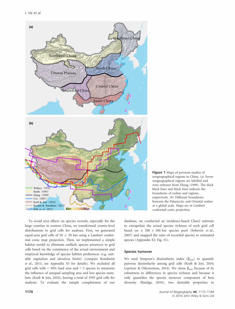
Traditionally, China has been divided into seven broad
zoogeographical regions: Northeast China, North China,
Northwest China, the Tibetan Plateau, Central China, South-
west China and South China (Zhang, 1999; Fig. 1a). Most
previous zoogeographical schemes were based on expert
opinions (Cheng & Chang, 1956; Zhang & Zhao, 1978;
Zhang, 1998). Recently, the number of quantitative zoogeo-
graphical studies of China has increased rapidly, but most of
these have been lineage-specific (Xie et al., 2004; Chen & Bi,
2007; P€ackert et al., 2012), used coarse grain sizes (Xiang
et al., 2004; Heiser & Schmitt, 2013), or focussed on the local
scale (Chen et al., 2008). Studies have been based on diverse
area sizes and operational geographical units (e.g. physio-
graphical regions), varying taxa and different methods, result-
ing in ongoing disagreement. Consequently, a quantitative
national-scale investigation based on fine resolution data for
several lineages of terrestrial vertebrates is needed to
understand and update the zoogeographical regions of China.
Global zoogeographical regionalizations traditionally
divided China into the Palaearctic and Oriental realms
(Sclater, 1858; Wallace, 1876; Cox, 2001; Kreft & Jetz, 2010;
Morrone, 2015). Wallace (1876) placed the Palaearctic-
Oriental boundary at c. 30° N, and most expert-based
schemes followed this proposition with only slight modifica-
tions (Zhang, 1999; Cox, 2001; Fig. 1b). Using comprehen-
sive mammal distribution data and clustering algorithms,
Kreft & Jetz (2010) suggested a more northern placement of
this boundary at c. 40° N (see also Rueda et al., 2013),
whereas Proches� & Ramdhani (2012) suggested that a much
more southern location (at c. 20° N). Most recently, by inte-
grating species distributions and phylogenetic information,
Holt et al. (2013) proposed a new ‘Sino-Japanese’ realm to
lie between c. 25° N and 40° N in East Asia (including most
of eastern China, the Tibetan Plateau and Japan). In sum,
there is considerable disagreement among previous studies
(Fig. 1b), and the location of the East Asian boundary
between the Palaearctic and Oriental realms has oscillated
c. 2000 km from c. 20° N to 40° N.
Here, we used the quantitative framework described in
Kreft & Jetz (2010) to identify zoogeographical regions for
China based on a large species dataset of terrestrial verte-
brates and specifically investigated the location of the
Palaearctic-Oriental boundary. We used multiple regression
analyses to investigate the current and historical environmen-
tal drivers shaping zoogeographical regions. Finally, we
evaluated the level of cross-taxon congruence.
MATERIALS AND METHODS
Species distribution data
Species distributions of terrestrial vertebrates (amphibians,
reptiles, birds and mammals) for the 2499 counties of
China (based on a 1 : 250,000 national digitized database
updated in 2002 with a median range size of 1780 km2 and
5% and 95% quartiles of 252 km2 and 12,771 km2, respec-
tively) were compiled from (1) The First National Terres-
trial Animal Survey database (11,165 species records) and
76 Nature Reserve Reports (13,918 species records), both of
which were obtained from the State Forestry Administra-
tion and (2) books on fauna published before 2012 (72,853
species records), including Fauna of China (20 issues of 28
volumes for terrestrial vertebrates), as well as national and
regional atlases and books (a full reference list is provided
in Appendix S1 in the Supporting Information). In total,
we included 97,936 species-county records in this study.
We excluded all bats (120 species) because of incomplete
distribution information as well as all birds with only win-
tering ranges in China (156 species) because their migratory
behaviour is of limited usefulness for regionalization
(Rueda et al., 2013). This resulted in a total of 2102 species
for analysis, including 329 amphibians, 361 reptiles, 1008
birds and 404 mammals (see Appendix S2: Table S1 for
details). Additionally, combining the species distributions in
each genus and family produced higher taxonomic rank
analyses.
Journal of Biogeography 44, 1172–1184ª 2016 John Wiley & Sons Ltd
1173
Zoogeographical regions of China
To avoid area effects on species records, especially for the
large counties in western China, we transformed county-level
distributions to grid cells for analyses. First, we generated
equal-area grid cells of 50 9 50 km using a Lambert confor-
mal conic map projection. Then, we implemented a simple
habitat model to eliminate unlikely species presences in grid
cells based on the consistency of the actual environment and
empirical knowledge of species habitat preferences (e.g. suit-
able vegetation and elevation limits) (compare Rondinini
et al., 2011; see Appendix S3 for details). We excluded all
grid cells with < 50% land area and < 5 species to minimize
the influence of unequal sampling area and low species num-
bers (Kreft & Jetz, 2010), leaving a total of 3595 grid cells for
analyses. To evaluate the sample completeness of our
database, we conducted an incidence-based Chao2 estimate
to extrapolate the actual species richness of each grid cell
based on a 200 9 200 km species pool (Sober�on et al.,
2007) and mapped the ratio of recorded species to estimated
species (Appendix S2: Fig. S1).
Species turnover
We used Simpson’s dissimilarity index (bsim) to quantify
pairwise dissimilarity among grid cells (Kreft & Jetz, 2010;
Leprieur & Oikonomou, 2014). We chose bsim because of its
robustness to differences in species richness and because it
only quantifies the species turnover component of beta
diversity (Baselga, 2010), two desirable properties in
Wallace 1876Smith 1983Zhang 1999Cox 2001Kreft & Jetz 2010Proches & Ramdhani 2012Holt 2013et al HighLow
Northwest China
Tibetan Plateau
Southwest China
South China
Central China
North China
Northeast China
(a)
(b)
Figure 1 Maps of previous studies ofzoogeographical regions in China. (a) Seven
zoogeographical regions are labelled and
were redrawn from Zhang (1999). The thickblack lines and black lines indicate the
boundaries of realms and regions,respectively. (b) Different boundaries
between the Palaearctic and Oriental realmsat a global scale. Maps are in Lambert
conformal conic projection.
Journal of Biogeography 44, 1172–1184ª 2016 John Wiley & Sons Ltd
1174
J. He et al.

bioregionalization (Kreft & Jetz, 2010). The bsim index calcu-
lates the species dissimilarity distance between two grid cells
as follows:
bsim ¼ 1� a
minðb; cÞ þ a
where a is the number of shared species and b and c are the
number of species unique to each grid cell. bsim ranges from
0 to 1, with smaller values indicating lower dissimilarity.
Cluster analysis
We applied unweighted pair-group method using arithmetic
averages (UPGMA) hierarchical clustering to the dissimilarity
matrix. UPGMA produces a dendrogram displaying the hier-
archical relationships of all grid cells and has been shown to
consistently perform best in global-scale biogeographical
regionalization (Kreft & Jetz, 2010). We assessed the perfor-
mance of UPGMA in transferring the dissimilarity matrices
into dendrograms using cophenetic correlation coefficients.
Three UPGMA results were produced and compared using
(1) grid-based species (genus/family) assemblages; (2) regio-
nal taxa lists of the grid-based outputs; and (3) weighted dis-
similarity matrices relative to the species numbers (0.35 for
amphibians, 0.30 for reptiles, 0.10 for birds and 0.25 for
mammals).
To compare our results to previous studies and to test for
levels of cross-taxon congruence, we used three criteria in
choosing a suitable cut-off point in the dendrograms: (1)
regions should not be disjunct; (2) the number of regions
should vary between 6 and 10, following Zhang (1999); and
(3) the number of regions should perform best with sum-of-
squares (Krzanowski & Lai, 1988).
Ordination analysis
Non-metric multidimensional scaling (NMDS) was performed
to investigate whether a zoogeographical transition zone exists
in eastern China. Grid cells in the NMDS ordination plots
were coloured based on UPGMA cluster membership to visu-
alize the relative distance between zoogeographical regions.
Additionally, we plotted external environmental factors as vec-
tors onto NMDS plots (Gonz�alez-Orozco et al., 2013) to
detect underlying relationships between faunistic dissimilarity
and dominant environmental gradients. We used stress values
to assess the fit between the NMDS and the original dissimilar-
ity matrix. Stress values ranged from 0 to 1, with smaller values
indicating better NMDS results. Finally, the NMDS results
were rotated and rescaled to maximize comparability with
geography.
Environmental variables
We investigated four main categories of predictor variables
that potentially determine zoogeographical regions: (1) cur-
rent climate (Buckley & Jetz, 2008), (2) past climate change
(Dobrovolski et al., 2012), (3) vegetation (Mac Nally et al.,
2004) and (4) geological processes (Badgley, 2010). Current
climatic predictors included mean annual temperature (°C;MAT), mean annual precipitation (mm; PRE), temperature
seasonality (°C; TS) and precipitation seasonality (%; PS).
The average climatic conditions for each grid cell were
derived from the WorldClim dataset (~1 9 1 km resolution;
Hijmans et al., 2005; http://www.worldclim.org). Past climate
change predictors included temperature change (°C, TC) andprecipitation change (°C, PC), which were calculated
according to the standard deviation of four climate periods:
Current (1950–2000), Last Interglacial (LIG; ~120,000–140,000 yr bp), Last Glacial Maximum (LGM; ~21,000 yr
bp) and Mid-Holocene (~6000 yr bp). Dominant vegetation
types were sourced from the vegetation map of China
(Zhang et al., 2007; Appendix S2: Fig. S2). Topographic pre-
dictors, including mean elevation (m, ELE) and elevation
range (m, ELER), were derived from digital elevation data
(~90 9 90 m resolution) downloaded from the Consortium
for Spatial Information (http://www.cgiar-csi.org/data/
srtm-90m-digital-elevation-database-v4-1). Tectonic plates
(TEC) were obtained from Kusky et al. (2007)
(Appendix S2: Fig. S3) and were digitized using a geographi-
cal information system (ArcInfo version 9.3., ESRI, 2008).
These data resulted in eight continuous and two categorical
variables.
Among the 28 pairwise Pearson correlations of the eight
continuous predictors (Appendix S2: Table S2), only two
(MAT and PRE; MAT and ELE) were above the commonly
used threshold of |r| = 0.7 (Dormann et al., 2013). Addition-
ally, we selected predictors based on the Akaike information
criterion (AIC) and R2 values that were not affected by
collinearity (Burnham & Anderson, 2002; Cohen et al.,
2003). All continuous variables were standardized to have a
mean of zero and a variance of one.
Drivers of zoogeographical regions
We used generalized linear models (GLMs) with multinomial
logit-link functions to model UPGMA group membership as
a multinomial response variable (Rueda et al., 2010). Models
including all possible combinations of the 10 variables were
calculated and model selection was based on corrected
Akaike’s information criterion (AICc) scores (Johnson &
Omland, 2004). We selected the best model according to the
commonly accepted criterion of DAICc < 2 (Burnham &
Anderson, 2002). Next, we used deviance partitioning to
identify the amount of independent and joint deviance
explained by each predictor (Rueda et al., 2010). Only
predictors retained in the best models were included.
Cross-taxon congruence
To evaluate the level of cross-taxon congruence, we first car-
ried out separate clustering analyses for the four individual
lineages to visualize spatial patterns. Next, we used Mantel
Journal of Biogeography 44, 1172–1184ª 2016 John Wiley & Sons Ltd
1175
Zoogeographical regions of China

tests (Mantel, 1967) to calculate the correlation coefficients
(rm) for pairs of dissimilarity matrices (bsim). Statistical sig-nificance was calculated with a Mantel Carlo permutation
test using 999 permutations. We used Kruskal–Wallis tests to
test for differences in geographical range sizes among the
four lineages which may cause differences in biogeographical
regionalizations. The geographical range size was measured
as the latitudinal extent and the longitudinal extent occupied
by each species (Gaston, 1996).
All analyses were conducted in r version 3.1.2 (R Develop-
ment Core Team, 2015), using the packages ‘vegan’ (Oksanen
et al., 2015), ‘betapart’ (Baselga et al., 2013), ‘NbClust’ (Char-
rad et al., 2014), ‘nnet’ (Venables & Ripley, 2002), ‘MuMIn’
(Barto�n, 2016) and ‘ecodist’ (Goslee & Urban, 2007).
RESULTS
Zoogeographical regions
The UPGMA clustering of grid-based species assemblages
yielded 10 major zoogeographical regions for China (Fig. 2a,
b): South China, the Yungui Plateau, Taiwan, North China,
Northeast China, the Inner Mongolia Plateau, Northwest
China, the Longzhong Plateau, the Tibetan Plateau and East
Himalaya. A high cophenetic correlation coefficient (r > 0.8)
indicated good agreement between cluster assignments and
the original bsim matrix. The grid cell assemblages of the 10
major zoogeographical regions included a range of bsim val-
ues of c. 0.93–0.67 (Fig. 2a,b). The boundary between the
traditionally accepted Palaearctic and Oriental realms in east-
ern China (c. 30° N) emerged at a height of c. 0.84 in the
dendrogram (Fig. 2a: node 6). Taiwan merged with the
nearby mainland at c. 0.91 (Fig. 2a: node 8) and the regions
of western China and eastern China merged last at c. 0.93
(Fig. 2a: node 9). Two small clusters, coloured with grey and
nested among South China and North China, were excluded
from further discussion.
Clustered regions were also separated in the NMDS
(Fig. 2c). The stress value of 0.17 indicated relatively good
projection of the dissimilarity matrix into the two-dimen-
sional ordination space. The change in faunistic composition
in western China was discontinuous: Northwest China, the
Tibetan Plateau, the Longzhong Plateau and East Himalaya
were distinctly separated from each other (Fig. 2b,c). Con-
versely, there was a gradual transition in faunistic composi-
tion in eastern China. In particular, grid cells belonging to
North China largely overlapped with grid cells belonging to
Northeast China and South China.
The UPGMA clustering of grid cell assemblages based on
a higher taxonomic level showed some differences. At the
family level, only four large clusters were identified, but the
major separation between western China and eastern China
remained valid (Fig. 3a). At the genus level, clustering
showed geographical patterns similar to those at the species
level with two exceptions: the Longzhong Plateau and East
Himalaya merged and the Yungui Plateau and South China
merged at the genus level (compare Fig. 3b with Fig. 2b),
yielding eight major regions.
Drivers of zoogeographical regions
When relating environmental factors to the NMDS ordina-
tion, mean annual precipitation, temperature seasonality and
mean elevation emerged as the most important factors
(Fig. 2c). The vector for PRE separated grid cells located in
Southeast China, where the climate was strongly monsoonal
with high precipitation from grid cells in the very dry envi-
ronment of Northwest China. Alpine environments in the
TS
MAT
PREPC
ELE
ELER
PS TC
1
1
0 NMDS 1
NM
DS
2
7
43
Taiwan
South China
Yungui Plateau
Northeast China
North China
East Himalaya
Tibetan Plateau
Longzhong Plateau
Northwest China
Inner Mongolia Plateau
sim10.65
(b)(a)
TS
MAT
PREPC
ELE
ELER
PS TC
10 NMDS 1
NM
DS
2
0 8 0 6 0 4 0 2 0.01 0 (c)
species 5
28
9
6
5
1
Figure 2 Zoogeographical regionalization for the terrestrial vertebrates of China. (a) Dendrogram from UPGMA hierarchical clustering
of grid-based species assemblages. The phenon line indicates the cut-off location and nine main nodes are labelled in sequence. Thecophenetic correlation coefficient is 0.82. (b) Map showing the results from UPGMA clustering on a 50 9 50 km grid. The map is in
Lambert conformal conic projection. (c) NMDS ordination based on the bsim dissimilarity matrix of grid cell assemblages and the stressvalue is 0.17. The grid cells with less than five species are not shown in the ordination. The NMDS result is rotated and rescaled to
maximize consistency with geography. Eight continuous environmental variables are fitted to interpret the ordination. All variables inthis analysis are highly significant (P < 0.001).
Journal of Biogeography 44, 1172–1184ª 2016 John Wiley & Sons Ltd
1176
J. He et al.

Genus
Taiwan
Yungui Plateau
East Himalaya
Northwest China
Northeast China
Tibetan Plateau
Inner Mongolia Plateau
North China
sim10
0 0 0 2 0 4 0 6 0 8
taxa 5
Family
South China
Northwest China
Northeast China
Tibetan Plateau &Inner Mongolia Plateau
0 0 0 1 0 2 0 3 0 50 4(a)
(b)
Longzhong Plateau &
South China &
Figure 3 Dendrograms and maps of UPGMA clustering for terrestrial vertebrates at the (a) family and (b) genus levels. Cophenetic
correlation coefficients for cluster analyses are 0.50 for the family level and 0.73 for the genus level. The maps are based on a50 9 50 km grid and are in Lambert conformal conic projection.
Journal of Biogeography 44, 1172–1184ª 2016 John Wiley & Sons Ltd
1177
Zoogeographical regions of China

Tibetan Plateau were characterized by positive mean eleva-
tion vectors and elevation range vectors.
In single-predictor GLMs (Table 1), factors reflecting vege-
tation types explained the highest amounts of deviance
(57%). Geological processes ranked high in explaining
deviance, with tectonic plates ranking second (55% of the
deviance explained) and mean elevation ranking fourth (42%
of the deviance explained). Current climate, which included
temperature seasonality, mean annual precipitation and
mean annual temperature, also explained large amounts of
the deviance (45%, 40% and 39%, respectively). When all
ten factors were considered in multiple regression GLMs
(Table 1, Appendix S2: Table S3), the best model
(DAICc < 7; Akaike weight = 0.98) explained 90% of the
deviance and included all predictors except vegetation types,
mean annual temperature and precipitation change.
According to the deviance partitioning analysis (Fig. 4),
geological processes accounted for most of the deviance
explained independently (8.3%) followed by current climate
(7.1%). These two groups of predictors also jointly explained
the highest percentage of deviance (61.0%). Past climate
change explained only 0.8% of deviance independently and
7.6% of deviance jointly with current climate and geological
processes.
Cross-taxon congruence
Mantel tests on the bsim matrices showed the highest correla-
tion between mammals and birds (rm = 0.74, P < 0.001), fol-
lowed by mammals and reptiles (rm = 0.71, P < 0.001), and
the lowest correlation between mammals and amphibians
(rm = 0.58, P < 0.001; Table 2). When controlling for spatial
autocorrelation (geographical distance), the pairwise partial
correlation coefficients were weaker yet highly significant
(P < 0.001). The combined dissimilarity matrix corre-
sponded strongly to mammals and birds (both rm = 0.91)
and represented all four lineages well (all rm > 0.75,
P < 0.001). The four vertebrate lineages showed significant
differences in range size (Kruskal–Wallis test, P < 0.001;
Fig. 5). Mammals and birds occupied relatively larger spatial
extents (the medians were 13.4 longitudes, 8.3 latitudes for
mammals and 13.4 longitudes, 8.7 latitudes for birds) than
reptiles and amphibians (the medians were 8.4 longitudes,
5.8 latitudes for reptiles and 3.5 longitudes, 2.9 latitudes for
amphibians). Moreover, the dendrograms and maps of the
four individual groups yielded noteworthy differences in the
topologies and assignments of zoogeographical regions (see
Table 1 Results from generalized linear models investigating the
effects of current climate, past climate change, vegetation andgeological processes on zoogeographical regions in China.
Variables Best model
Variable
importance R2
Mean annual temperature – 0.02 0.39
Mean annual precipitation + 1 0.40
Temperature seasonality + 1 0.45
Precipitation seasonality + 1 0.18
Temperature change + 1 0.14
Precipitation change – <0.01 0.22
Vegetation types – <0.01 0.57
Mean elevation + 1 0.42
Elevation range + 0.98 0.09
Tectonic elements + 1 0.55
AICc 1671.7 – –Akaike weight 0.98 – –R2
model 0.90 – –
‘+’ indicates variables included in the best model (DAICc ≤ 2); AICc
is Akaike’s information criterion corrected for a small sample size;
Akaike weight is the probability of one model being in favoured over
alternative models; R2model is the deviance explained by the best
model; Variable importance is the relative importance of each vari-
able calculated by the sum of the Akaike weight of models including
them; R2 is the deviance explained by each factor in single-predictor
models.
0.8
7.1 8.361.0
2.6 3.17.6
U=9.5
C G
PFigure 4 Partitioned deviances of the three main categories
used in investigating the assignment of the zoogeographicalregions. Predictors are derived from the best model in GLMs: C
(current climate: mean annual precipitation + precipitationseasonality + temperature seasonality); G (geological processes:
mean elevation + elevation range + tectonic elements); P (pastclimate change: temperature change); U (unexplained).
Table 2 Mantel correlation coefficients (rm) among pairs of
taxa measured by Mantel (above diagonal) and partial Mantel(below diagonal) tests based on bsim matrices. Spatial
autocorrelation was accounted for in the partial Mantel test byincluding a geographical distance matrix. All tests were highly
significant (P < 0.001).
Combined Mammals Birds Reptiles Amphibians
Combined – 0.91 0.91 0.81 0.76
Mammals 0.86 – 0.74 0.71 0.58
Birds 0.86 0.62 – 0.66 0.63
Reptiles 0.70 0.56 0.47 – 0.60
Amphibians 0.68 0.43 0.51 0.44 –
Journal of Biogeography 44, 1172–1184ª 2016 John Wiley & Sons Ltd
1178
J. He et al.

Appendix S2: Fig. S4 for details). The dendrograms of mam-
mals and birds divided China into a western part and an
eastern part, whereas the dendrograms of reptiles split the
Tibetan Plateau and the dendrograms of amphibians spilt
Taiwan from the rest of China. Reptiles and amphibians
tended to have more divided regions in the tropical–subtrop-ical zone, but the configurations of regions for mammals
and birds were more balanced.
DISCUSSION
Zoogeographical regions
The zoogeographical regions revealed by UPGMA clustering
(Fig. 2b) were largely consistent with the expert-based
scheme of Zhang (1999) (Fig. 1a). For example, Northeast
China and North China matched well with Zhang (1999),
and Northwest China and the Inner Mongolia Plateau
combined coincided with Zhang’s Northwest China region
(compare Fig. 2b to Fig. 1a). However, some discrepancies
emerged. First, we did not find support for a distinction
between South China and Central China (Fig. 1a, Fig. 2),
and the UPGMA only identified a single South China region
(Fig. 2). This finding was consistent with other mammalian
studies claiming that the boundary between Central China
and South China is not significant and that Central China is
best considered as part of a larger South China region (Xiang
et al., 2004). Second, Taiwan was previously regarded as a
subregion of South China (Fig. 1a; Zhang, 1999). However,
UPGMA clustering identified Taiwan as a distinct region due
to the island’s unique fauna and high levels of endemism
(Lei et al., 2007; Fig. 2a,b). The distinct position of Taiwan
was detected for the combined dataset, for each individual
vertebrate group, and occurred at the species and genus
levels (Figs 2 & 3b; Appendix S2: Fig. S4). Although the rela-
tionships between Taiwan and South China were closer at
the genus level, the status of Taiwan as a distinct region
appears to be justified. High avian endemism for Taiwan has
been reported before (Lei et al., 2003), and recent phyloge-
netic studies on birds provide evidence that a considerable
number of Taiwanese endemic species originated from Indo-
china rather than from the nearby mainland (Wang et al.,
2013; Chen et al., 2015), supporting Taiwan as a distinct
region. Third, and also unexpectedly, the Longzhong Plateau,
which was not previously regarded as a distinct region, was
clearly separated from the Tibetan Plateau in hierarchical
clustering (Fig. 2). Even at the genus level, the combined
Longzhong Plateau and East Himalaya regions were identi-
fied (Fig. 3b), indicating distinct fauna from surrounding
regions. This distinction occurred because the Longzhong
Plateau region is located at the point of convergence of lin-
eages from the north–south and east–west and is character-
ized by a uniquely mixed species composition instead of
high levels of endemism (Appendix S2: Table S4). Such an
area may also be considered a transition zone (Ferro & Mor-
rone, 2014; Morrone, 2015), but following the classical
regionalization system, we regard the Longzhong Plateau as
an independent region.
Noteworthily, some differences emerged when contrasting
the three UPGMA results produced by the grid cells
(Fig. 2a), regional lists (Appendix S2: Fig. S6a) and weighted
dissimilarity matrix (Appendix S2: Fig. S6b). For instance,
the Yungui Plateau recognized in the grid-based analysis was
divided into three parts in the weighted dissimilarity matrix
analysis (Appendix S2: Fig. S6b). Due to greater weights for
amphibians and reptiles, species turnover in the combined
weighted dissimilarity matrix produced sharper changes
between tropical and mountainous areas and resulted in
unbalanced assignments of zoogeographical regions (temper-
ate regions were much bigger than tropical regions). There-
fore, unless dealing with a specific question related to the
impact of weighted species numbers or weighted species
occurrences on bioregionalization, the traditionally accepted
grid-based approach without weights is preferable (Linder
0 10 20 30 40 50 60
010
2030
40
Longitude
Latit
ude
Mammals
Birds
Reptiles
Amphibians
Figure 5 Species geographical range sizesfor each lineage in China. Geographical
range size is estimated as the latitudinalextents and longitudinal extents occupied by
each species. Ellipses indicate 95%confidence intervals. Vertical and horizontal
box-and-whisker plots stand for the
latitudinal extents and longitudinal extentsoccupied by the four groups. Outliers are
not shown. The range sizes (i.e. latitudinalextents and longitudinal extents) between
endotherms and ectotherms are significantlydifferent (Kruskal–Wallis test, P < 0.001).
Journal of Biogeography 44, 1172–1184ª 2016 John Wiley & Sons Ltd
1179
Zoogeographical regions of China
et al., 2012). Furthermore, the Yungui Plateau had a closer
affinity to South China in the grid-based result, whereas in
the analysis based on regional lists, the Yungui Plateau was
closer to East Himalaya. This may be attributed to the fact
that zoogeographical regions based on whole regional lists
share more linking species than single grid cells (Kreft & Jetz,
2010). Although there were inevitably discrepancies among
the different approaches, the assignments of the main zoo-
geographical regions were consistent. The most important
boundary, at c. 105° E, first split western China and eastern
China, followed by the latitudinal boundary at c. 30° E,
which split eastern China into South China and North
China. Next, western China was separated into Northwest
China, the Tibetan Plateau and East Himalaya. Taiwan was
identified consistently in all approaches. We, therefore, advo-
cate the grid-based scheme because of its objective opera-
tional geographical units (Kreft & Jetz, 2010) and equal
weight for each individual species (Linder et al., 2012).
Palaearctic-Oriental boundary
East Asia is a region with complex interchange between
tropical Oriental and temperate Palaearctic faunas (Proches�& Ramdhani, 2012; Morrone, 2015). Thus, establishing a
discrete boundary between these two realms is very difficult
and has resulted in many different proposals owning to dif-
ferences in methods, taxa, taxonomic ranks, grain sizes or
spatial extents (Wallace, 1876; Hoffmann, 2001; Kreft & Jetz,
2010; Heiser & Schmitt, 2013; Holt et al., 2013). According
to our results, however, the traditionally accepted boundary
at c. 30° N only emerged at bsim = c. 0.84, whereas the
boundary between western and eastern China emerged at
bsim = c. 0.93 and was located at c. 105° E, indicating that
northern and southern China had smaller dissimilarity than
western and eastern China (Fig. 2a). A strong east–west sep-aration was also supported at a higher taxonomic rank
(Fig. 3). This situation may be attributed to the interchange
between northern and southern fauna caused by unstable
climate change in eastern China during the Pleistocene per-
iod (Norton et al., 2011). However, due to the elevational
barrier of the Tibetan Plateau and the very dry environment
of Northwest China, species dissimilarity between eastern
China and western China is greater. Therefore, as hierarchi-
cal clustering first distinguished eastern China and western
China (Fig. 2a,b), we suggest that the Palaearctic-Oriental
boundary in China is more likely to be of north–south ori-
entation than the traditionally accepted east–west orienta-
tion. This finding is generally consistent with the global
scheme proposed by Kreft & Jetz (2010) (compare Fig. 2
and Fig. 3 to Fig. 1).
Drivers of zoogeographical regions
Current climate emerged as a major determinant of zoogeo-
graphical regions in general and as a determinant of the
strong east–west differentiation in particular. These results
were consistent with previous findings by Wang et al. (2012)
who found that environmental effects determined longitudi-
nal patterns of woody plants in China. Because of its pro-
nounced aridity, Northwest China is inhabited mainly by
drought-tolerant species, and the Tibetan Plateau is charac-
terized by a fauna adapted to high altitudes, excessive
drought, severe coldness and low oxygen levels (Yin, 1994).
South China, in contrast, harbours numerous arboreal verte-
brate species that are confined to the subtropical zone, which
reaches its limit at ~30 °N in eastern China (Zhang, 1999).
Our results also highlight a strong role of geological pro-
cesses in shaping zoogeographical regions. For instance,
although environmental conditions in Taiwan are similar to
those in the nearby mainland (Appendix S2: Fig. S5), Taiwan
was clearly identified as a distinct region due to the geo-
graphical isolation caused by its island setting. Tectonic plate
membership, as a surrogate for historical effects (Keith et al.,
2013), had high R2 value in our single-predictor models and,
together with the two elevation-related variables, indepen-
dently explained the highest deviance in the multi-predictor
GLMs (Table 1, Fig. 4). Tectonic plates and continent
boundaries are important in understanding the underlying
relationships between geological events and the formation of
zoogeographical regions (Wallace, 1876; Kreft & Jetz, 2010),
but their effect on geological history at the regional scale is
less clear. Our faunistic regions showed a good match to
geological elements in China. For example, the border of the
Tibetan Plateau region was strikingly similar to the borders
of the Alpine–Himalaya orogen, the Songpan Ganzi orogen
and the Central China orogen. South China matched the
Yangtze Craton and the Cathaysia Craton, and North China
matched to the North China Craton (Kusky et al., 2007;
compare Fig. 2b to Appendix S2: Fig. S3).
Cross-taxon congruence
Congruence between endotherms and ectotherms was rela-
tively low and the individual UPGMA dendrograms showed
considerable differences (Table 2; Appendix S2: Fig. S4).
These patterns may be attributed to different basic underly-
ing traits, particularly sensitivity to environmental conditions
(Buckley & Jetz, 2007), range size and dispersal ability
(Rueda et al., 2010; Fig. 5). Ectotherms are assumed to have
higher sensitivity to climatic conditions (Buckley & Jetz,
2007) and lower dispersal ability (Fig. 5). Therefore, zoogeo-
graphical regions based on ectotherms tended to be smaller
in tropical–subtropical and mountainous areas (e.g. the Yun-
gui Plateau) and tended to be bigger in temperate and flat
areas (e.g. Northwest China) (Appendix S2: Fig. S4; compare
Chen & Bi, 2007). Mammals and birds, in contrast, have lar-
ger ranges (Pimm et al., 2014) and were less influenced by
the environment. Consequently, changes in species composi-
tion were more gradual (Appendix S2: Table S4). Together,
these results explain the low congruence between endotherms
and ectotherms. Interestingly, the regionalization for mam-
mals generally corresponded most closely to the combined
Journal of Biogeography 44, 1172–1184ª 2016 John Wiley & Sons Ltd
1180
J. He et al.

regionalization (compare Appendix S2: Fig. S4a to Fig. 2b;
Table 2), supporting the use of mammals as a model group
for zoogeographical regionalization (Wallace, 1876; Hagmeier
& Stults, 1964; Smith, 1983; Heikinheimo et al., 2007; Kreft
& Jetz, 2010; Escalante et al., 2013).
Potential caveats
Our study has several limitations. First, grid cells with less
than five species (particularly for amphibians and reptiles)
caused by either ecologically restricted environments or defi-
cient sampling would bias our results. Distributions derived
from field surveys and faunistic books were also prone to
spatial differences in sampling effort (compare Meyer et al.,
2015). In particular, vertebrates sampling was incomplete in
southeastern China and the North China Plain (Yang et al.,
2013) due to the low collection intensity (Appendix S2:
Fig. S1). The robustness of the simple habitat model that
converted county-level records into grid cells also repre-
sented a potential problem. Fine-scale mapping of species
distributions in China is a challenging and ongoing mission
(Yang et al., 2013), but despite these shortcomings, our
study was the first to use a grid-based database consisting of
nearly all terrestrial vertebrates to delineate zoogeographical
regions of China. Second, similarity measures might fail to
reveal historical relationships among zoogeographical regions
(Escalante et al., 2013), meaning that regions obtained by
cluster analyses lack evolutionary support. For historical bio-
geography, analyses under the criterion of endemism (e.g.
parsimony analysis of endemicity and endemicity analysis)
should be used (Morrone, 2015). It should be noted that to
understand the current spatial patterns of biodiversity in
China, we defined a biogeographical region as a regional spe-
cies pool with a maximum internal similarity and with maxi-
mum differences compared with other regions (Kreft & Jetz,
2010; Linder et al., 2012). From this point of view, biogeo-
graphical regionalizations based on species (genus/family)
similarity proved to be valid (Cox, 2010; Kreft & Jetz, 2010;
Proches� & Ramdhani, 2012). Finally, from a methodological
point of view, although hierarchical clustering is an effective
tool for bioregionalization, it has an inherent limitation in
dealing with transition zones (Kreft & Jetz, 2013). Refining
and combining different approaches, such as clustering (Kreft
& Jetz, 2010), ordination (Williams et al., 1999) and network
analyses (Vilhena & Antonelli, 2015), are promising for
future studies.
CONCLUSIONS
Biogeographical regionalizations, based on detailed species
distributions from different lineages and multivariate tech-
niques, provide new insights into biogeography and put bio-
geography on a quantitative footing. Here, we used a
quantitative framework and proposed an updated scheme for
the zoogeographical regions of China, a country with out-
standing vertebrate diversity.
Our study yielded four main results: (1) In contrast to pre-
vious studies, we found support for Central China being a
part of South China, and the Longzhong Plateau and Taiwan
were identified as two new regions. (2) Overall, our results
provide ample support for a broad biogeographical transition
zone in East Asia and provide a fresh, regional perspective
suggesting that the Palaearctic-Oriental boundary inside
China has a more strongly south–north orientation rather
than the conventionally accepted east–west orientation. (3)
The zoogeographical regions for China are significantly influ-
enced by complex interplay between topography, geological
context and current climate. (4) Although the configurations
of zoogeographical regions for the four lineages showed some
discrepancies, our scheme held up well for each group.
ACKNOWLEDGEMENTS
We gratefully thank Peter Linder, Brett Riddle, Juan J.
Morrone, Syd Ramdhani and an anonymous referee for their
reviews and constructive comments on an earlier version of
this manuscript. We thank Y.C. Long and X. Liu for valuable
discussions and comments that substantially improved this
manuscript. We also thank S.L. Lin, Y. Xu, C. Meyer and A.
Stein for technical assistance and helpful suggestions. H.K.
acknowledges funding from the German Research Founda-
tion (DFG) and the University of G€ottingen within the scope
of the Excellence Initiative. This study was a part of J.H.’s
Master’s programme partly supported by State Forestry
Administration of P.R. China.
REFERENCES
Badgley, C. (2010) Tectonics, topography, and mammalian
diversity. Ecography, 33, 220–231.Barto�n, K. (2016) MuMIn: multi-model inference. R package
version 1.15.6. Available at: http://CRAN.R-project.org/
package=MuMIn
Baselga, A. (2010) Partitioning the turnover and nestedness
components of beta diversity. Global Ecology and Biogeog-
raphy, 19, 134–143.Baselga, A., Orme, D., Villeger, S., Bortoli, J.D. & Leprieur,
F. (2013) betapart: partitioning beta diversity into turnover
and nestedness components. R package version 1.3. Avail-
able at: http://CRAN.R-project.org/package=betapart
Buckley, L.B. & Jetz, W. (2007) Environmental and historical
constraints on global patterns of amphibian richness. Pro-
ceedings of the Royal Society B: Biological Sciences, 274,
1167–1173.Buckley, L.B. & Jetz, W. (2008) Linking global turnover of
species and environments. Proceedings of the National
Academy of Sciences USA, 105, 17836–17841.Burnham, K.P. & Anderson, D.R. (2002) Model selection and
multimodel inference: a practical information-theoretic
approach, 2nd edn. Springer, New York.
Carstensen, D.W., Dalsgaard, B., Svenning, J.-C., Rahbek, C.,
Fjelds�a, J., Sutherland, W.J. & Olesen, J.M. (2012)
Journal of Biogeography 44, 1172–1184ª 2016 John Wiley & Sons Ltd
1181
Zoogeographical regions of China

Biogeographical modules and island roles: a comparison of
Wallacea and the West Indies. Journal of Biogeography, 39,
739–749.Charrad, M., Ghazzali, N., Boiteau, V. & Niknafs, A. (2014)
NbClust: an R package for determining the relevant num-
ber of clusters in a data set. Journal of Statistical Software,
61, 1–36.Chen, Y. & Bi, J. (2007) Biogeography and hotspots of
amphibian species of China: implications to reserve
selection and conservation. Current Science, 92, 480–489.
Chen, L., Song, Y. & Xu, S. (2008) The boundary of
Palaearctic and Oriental realms in western China. Progress
in Natural Science, 18, 833–841.Chen, D., Chang, J., Li, S.H., Liu, Y., Liang, W., Zhou, F.,
Yao, C.T. & Zhang, Z. (2015) Was the exposed continental
shelf a long-distance colonization route in the ice age? The
Southeast Asia origin of Hainan and Taiwan partridges.
Molecular Phylogenetics and Evolution, 83, 167–173.Cheng, T. & Chang, Y. (1956) On tentative scheme for divid-
ing zoogeographical regions of China. Acta Geographica
Sinica, 22, 93–109 (in Chinese).
Cohen, J., Cohen, P., West, S.G. & Aiken, L.S. (2003) Applied
multiple regression/correlation analysis for the behavioral
sciences. Lawrence Erlbaum Associates, Hillsdale, New Jersey.
Cox, C.B. (2001) The biogeographic regions reconsidered.
Journal of Biogeography, 28, 511–523.Cox, C.B. (2010) Underpinning global biogeographical
schemes with quantitative data. Journal of Biogeography,
37, 2027–2028.Dobrovolski, R., Melo, A.S., Cassemiro, F.A.S. & Diniz-Filho,
J.A.F. (2012) Climatic history and dispersal ability explain
the relative importance of turnover and nestedness com-
ponents of beta diversity. Global Ecology and Biogeography,
21, 191–197.Dormann, C.F., Elith, J., Bacher, S., Buchmann, C., Carl, G.,
Carr�e, G., Marqu�ez, J.R.G., Gruber, B., Lafourcade, B. &
Leit~ao, P.J. (2013) Collinearity: a review of methods to
deal with it and a simulation study evaluating their perfor-
mance. Ecography, 36, 27–46.Escalante, T., Morrone, J.J. & Rodr�ıguez-Tapia, G. (2013)
Biogeographic regions of North American mammals based
on endemism. Biological Journal of the Linnean Society,
110, 485–499.ESRI (2008) ArcGIS 9.3. Environmental Systems Research
Institute Inc., Redlands, CA.
Favre, A., P€ackert, M., Pauls, S.U., J€ahnig, S.C., Uhl, D.,
Michalak, I. & Muellner-Riehl, A.N. (2015) The role of the
uplift of the Qinghai-Tibetan Plateau for the evolution of
Tibetan biotas. Biological Reviews, 90, 236–253.Ferro, I. & Morrone, J.J. (2014) Biogeographical transition
zones: a search for conceptual synthesis. Biological Journal
of the Linnean Society, 113, 1–12.Gaston, K.J. (1996) Species-range-size distributions: patterns,
mechanisms and implications. Trends in Ecology and Evo-
lution, 11, 197–201.
Gonz�alez-Orozco, C.E., Laffan, S.W., Knerr, N. & Miller, J.T.
(2013) A biogeographical regionalization of Australian
Acacia species. Journal of Biogeography, 40, 2156–2166.Goslee, S.C. & Urban, D.L. (2007) The ecodist package for
dissimilarity-based analysis of ecological data. Journal of
Statistical Software, 22, 1–19.Hagmeier, E.M. & Stults, C.D. (1964) A numerical analysis
of the distributional patterns of North American mam-
mals. Systematic Zoology, 13, 125–155.Hattab, T., Albouy, C., Ben Rais Lasram, F., Le Loc’h, F.,
Guilhaumon, F. & Leprieur, F. (2015) A biogeographical
regionalization of coastal Mediterranean fishes. Journal of
Biogeography, 42, 1336–1348.Heikinheimo, H., Fortelius, M., Eronen, J. & Mannila, H.
(2007) Biogeography of European land mammals shows
environmentally distinct and spatially coherent clusters.
Journal of Biogeography, 34, 1053–1064.Heiser, M. & Schmitt, T. (2013) Tracking the boundary
between the Palaearctic and the Oriental region: new
insights from dragonflies and damselflies (Odonata). Jour-
nal of Biogeography, 40, 2047–2058.Hijmans, R.J., Cameron, S.E., Parra, J.L., Jones, P.G. & Jarvis,
A. (2005) Very high resolution interpolated climate sur-
faces for global land areas. International Journal of Clima-
tology, 25, 1965–1978.Hoffmann, R.S. (2001) The southern boundary of the
Palaearctic realm in China and adjacent countries. Acta
Zoologica Sinica, 47, 121–131.Holt, B.G., Lessard, J.-P., Borregaard, M.K., Fritz, S.A., Ara�ujo,
M.B., Dimitrov, D., Fabre, P.-H., Graham, C.H., Graves,
G.R., Jønsson, K.A., Nogu�es-Bravo, D., Wang, Z., Whit-
taker, R.J., Fjelds�a, J. & Rahbek, C. (2013) An update of
Wallace’s zoogeographic regions of the world. Science, 339,
74–78.Johnson, J.B. & Omland, K.S. (2004) Model selection in
ecology and evolution. Trends in Ecology and Evolution,
19, 101–108.Keith, S.A., Baird, A.H., Hughes, T.P., Madin, J.S. & Con-
nolly, S.R. (2013) Faunal breaks and species composition
of Indo-Pacific corals: the role of plate tectonics, environ-
ment and habitat distribution. Proceedings of the Royal
Society B: Biological Sciences, 280, 20130818.
Kreft, H. & Jetz, W. (2010) A framework for delineating bio-
geographical regions based on species distributions. Journal
of Biogeography, 37, 2029–2053.Kreft, H. & Jetz, W. (2013) Comment on “An update of Wal-
lace’s zoogeographic regions of the world”. Science, 341, 343.
Krzanowski, W.J. & Lai, Y. (1988) A criterion for determin-
ing the number of groups in a data set using sum-of-
squares clustering. Biometrics, 44, 23–34.Kusky, T.M., Windley, B.F. & Zhai, M.-G. (2007) Tectonic
evolution of the North China Block: from orogen to cra-
ton to orogen. Geological Society, London, Special Publica-
tions, 280, 1–34.Lei, F.-M., Qu, Y.-H., Lu, J.-L., Liu, Y. & Yin, Z.-H. (2003)
Conservation on diversity and distribution patterns of
Journal of Biogeography 44, 1172–1184ª 2016 John Wiley & Sons Ltd
1182
J. He et al.

endemic birds in China. Biodiversity and Conservation, 12,
239–254.Lei, F.-M., Wei, G.-A., Zhao, H.-F., Yin, Z.-H. & Lu, J.-L.
(2007) China subregional avian endemism and biodiversity
conservation. Biodiversity and Conservation, 16, 1119–1130.Leprieur, F. & Oikonomou, A. (2014) The need for richness-
independent measures of turnover when delineating bio-
geographical regions. Journal of Biogeography, 41, 417–420.Linder, H.P., de Klerk, H.M., Born, J., Burgess, N.D., Fjelds�a,
J. & Rahbek, C. (2012) The partitioning of Africa: statisti-
cally defined biogeographical regions in sub-Saharan
Africa. Journal of Biogeography, 39, 1189–1205.Mac Nally, R., Fleishman, E., Bulluck, L.P. & Betrus, C.J.
(2004) Comparative influence of spatial scale on beta
diversity within regional assemblages of birds and butter-
flies. Journal of Biogeography, 31, 917–929.Mantel, N. (1967) The detection of disease clustering and a
generalized regression approach. Cancer Research, 27, 209–220.
Meyer, C., Kreft, H., Guralnick, R. & Jetz, W. (2015) Global
priorities for an effective information basis of biodiversity
distributions. Nature Communications, 6, 8221.
Morrone, J.J. (2009) Evolutionary biogeography: an integrative
approach with case studies. Columbia University Press,
New York.
Morrone, J.J. (2015) Biogeographical regionalisation of the
world: a reappraisal. Australian Systematic Botany, 28, 81–90.
Norton, C.J., Jin, C., Wang, Y. & Zhang, Y. (2011) Rethink-
ing the Palearctic-Oriental biogeographic boundary in
Quaternary China. Asian paleoanthropology (ed. by C.J.
Norton and D.R. Braun), pp. 81–100. Springer, New York.
Oksanen, J., Blanchet, F.G., Kindt, R., Legendre, P., Minchin,
P.R., O’Hara, R.B., Simpson, G.L., Solymos, P., Stevens,
M.H.H. & Wagner, H. (2015) vegan: community ecology
package. R package version 2.3-2. Available at: http://
CRAN.R-project.org/package=vegan.
P€ackert, M., Martens, J., Sun, Y., Severinghaus, L.L., Nazar-
enko, A.A., Ting, J., T€opfer, T. & Tietze, D.T. (2012) Hori-
zontal and elevational phylogeographic patterns of
Himalayan and Southeast Asian forest passerines (Aves:
Passeriformes). Journal of Biogeography, 39, 556–573.Pimm, S.L., Jenkins, C.N., Abell, R., Brooks, T.M., Gittle-
man, J.L., Joppa, L.N., Raven, P.H., Roberts, C.M. & Sex-
ton, J.O. (2014) The biodiversity of species and their rates
of extinction, distribution, and protection. Science, 344,
1246752.
Proches�, S�. & Ramdhani, S. (2012) The world’s zoogeo-
graphical regions confirmed by cross-taxon analyses.
BioScience, 62, 260–270.R Development Core Team (2015). R: a language and envi-
ronment for statistical computing. Version 3.1.2. R Founda-
tion for Statistical Computing, Vienna, Austria. Available
at: http://www.R-project.org/
Renner, S.S. (2016) Available data point to a 4-km-high
Tibetan Plateau by 40 Ma, but 100 molecular-clock papers
have linked supposed recent uplift to young node ages.
Journal of Biogeography, 43, 1479–1487.Rondinini, C., Di Marco, M., Chiozza, F., Santulli, G., Bais-
ero, D., Visconti, P., Hoffmann, M., Schipper, J., Stuart,
S.N., Tognelli, M.F., Amori, G., Falcucci, A., Maiorano, L.
& Boitani, L. (2011) Global habitat suitability models of
terrestrial mammals. Philosophical Transactions of the Royal
Society B: Biological Sciences, 366, 2633–2641.Rueda, M., Rodr�ıguez, M.�A. & Hawkins, B.A. (2010)
Towards a biogeographic regionalization of the European
biota. Journal of Biogeography, 37, 2067–2076.Rueda, M., Rodr�ıguez, M.�A. & Hawkins, B.A. (2013) Identi-
fying global zoogeographical regions: lessons from Wallace.
Journal of Biogeography, 40, 2215–2225.Sclater, P.L. (1858) On the general geographical distribution
of the members of the class Aves. Journal of the Proceed-
ings of the Linnean Society of London: Zoology, 2, 130–145.Smith, C.H. (1983) A system of world mammal faunal
regions. I. Logical and statistical derivation of the regions.
Journal of Biogeography, 10, 455–466.Sober�on, J., Jim�enez, R., Golubov, J. & Koleff, P. (2007)
Assessing completeness of biodiversity databases at differ-
ent spatial scales. Ecography, 30, 152–160.Venables, W.N. & Ripley, B.D. (2002) Modern applied statis-
tics using S, 4th edn. Springer, New York.
Vilhena, D.A. & Antonelli, A. (2015) A network approach
for identifying and delimiting biogeographical regions.
Nature Communications, 6, 6848.
Wallace, A.R. (1876) The geographical distribution of animals.
Harper & Brothers, New York.
Wang, W., McKay, B.D., Dai, C., Zhao, N., Zhang, R., Qu,
Y., Song, G., Li, S.-H., Liang, W., Yang, X., Pasquet, E. &
Lei, F. (2013) Glacial expansion and diversification of an
East Asian montane bird, the green-backed tit (Parus
monticolus). Journal of Biogeography, 40, 1156–1169.Wang, Z., Fang, J., Tang, Z. & Lin, X. (2012) Relative role of
contemporary environment versus history in shaping
diversity patterns of China’s woody plants. Ecography, 35,
1124–1133.Williams, P.H., Klerk, H.M. & Crowe, T.M. (1999) Interpret-
ing biogeographical boundaries among Afrotropical birds:
spatial patterns in richness gradients and species replace-
ment. Journal of Biogeography, 26, 459–474.Xiang, Z.-F., Liang, X.-C., Huo, S. & Ma, S.-L. (2004) Quan-
titative analysis of land mammal zoogeographical regions
in China and adjacent regions. Zoological Studies, 43, 142–160.
Xie, Y., MacKinnon, J. & Li, D. (2004) Study on biogeo-
graphical divisions of China. Biodiversity and Conservation,
13, 1391–1417.Yang, W., Ma, K. & Kreft, H. (2013) Geographical sampling
bias in a large distributional database and its effects on
species richness–environment models. Journal of Biogeogra-
phy, 40, 1415–1426.Yin, H. (1994) The palaeobiogeography of China. Oxford
University Press, Oxford.
Journal of Biogeography 44, 1172–1184ª 2016 John Wiley & Sons Ltd
1183
Zoogeographical regions of China

Zhang, Y. (1998) The second revision of zoogeographical
regions of China. Acta Zootaxonomica Sinica, 23, 207–222(in Chinese).
Zhang, R. (1999) China animal geography. Science Press,
Beijing (in Chinese).
Zhang, Y. & Zhao, K. (1978) On the zoogeographical regions
of China. Acta Zoologica Sinica, 24, 196–202 (in Chinese).
Zhang, D., Liu, F. & Bing, J. (2000) Eco-environmental effects
of the Qinghai-Tibet Plateau uplift during the Quaternary
in China. Environmental Geology, 39, 1352–1358.Zhang, X., Sun, S., Yong, S., Zhou, Z. & Wang, R. (2007)
Vegetation map of the People’s Republic of China
(1: 1,000,000). Geological Publishing House, Beijing (in
Chinese).
SUPPORTING INFORMATION
Additional Supporting Information may be found in the
online version of this article:
Appendix S1 Data source of species distributions.
Appendix S2 Additional information of analyses.
Appendix S3 Framework of habitat suitability model.
BIOSKETCH
Jiekun He is a PhD student with interests in biogeography
and biodiversity. He specifically focuses on distribution
patterns of terrestrial vertebrate and gradients of biodiversity.
Author contribution: H.K. and J.H. conceived the ideas for
this study; H.J., E.G., Z.W. and J.H. contributed the data;
J.H., H.K. and H.J. analysed the data; and J.H., H.K. and
H.J. led the writing.
Editor: Brett Riddle
Journal of Biogeography 44, 1172–1184ª 2016 John Wiley & Sons Ltd
1184
J. He et al.