The 2017 World Congress on Advances in Structural Engineering and Mechanics (ASEM17) Ilsan(Seoul), Korea, August 28 - September 1, 2017

1

PBEE in a Moderate-Seismicity Region: South Korea

*Han Seon Lee1)

1) School of Civil, Environmental and Architectural Engineering, Korea University,

Seoul 02841, Korea 1)

hslee@korea.ac.kr

ABSTRACT

Performance-Based Earthquake Engineering (PBEE) has been developed mainly for the region of high seismicity for the last three decades. Though abundant information on PBEE is available throughout the world, the application of this PBEE to the moderate-seismicity regions such as their maximum considered earthquake being less than magnitude 6.5 is not always straightforward because some portion of the PBEE may not be appropriate in these regions due to the environment different from the high-seismicity regions. This paper reviews the state-of-art in PBEE briefly. Then, the seismic hazard in moderate-seismicity regions including Korean Peninsula is introduced with its unique characteristics. With this seismic hazard, representative low-rise RC MRF structures and high-rise RC residential wall structures are evaluated by using PBEE approach. Also, the range of forces and deformations of the representative building structures in Korea is given. Based on these reviews, some ideas for the use of PBEE to improve the state-of-practice in moderate-seismicity regions are proposed.

1. INTRODUCTION The conventional engineering design in many fields has been conducted by

satisfying all the requirements in the codes corresponding to the field of engineering. We call this design procedure the design to the prescriptive codes.

Prescriptive earthquake design codes currently in use are based on the traditional design philosophy preventing structural and nonstructural elements of buildings from any damage in low-intensity earthquakes, limiting the damage in these elements to reparable levels in medium-intensity earthquakes, and preventing the overall or partial collapses of buildings in high-intensity earthquakes. After the 1994 Northridge and 1995 Kobe earthquakes, the structural engineering community realized that the almost of damage, economic loss due to downtime, and repair cost of the structure was unacceptably high even though those structures complied with available seismic codes based on the above traditional philosophy.

1)

Professor

Keynote Paper

2

This realization led to the development of the concept of the first-generation performance-based earthquake engineering (PBEE) through Vision 2000 report (SEAOC 1995) in the US where the performance-based earthquake design is defined as a design framework by designating the desired system performance at various intensity levels of seismic hazard. The designer and owner consult to select the desired combination of performance and hazard levels to use as design criteria. In subsequent documents of the first-generation PBEE such as ATC 40 (1996), FEMA 273(1996), FEMA 356(2000), and ASCE 41-13(2013), the element deformation and force acceptability criteria corresponding to the performance are specified for different structural and non-structural elements for linear, nonlinear, static, and dynamic analysis. These criteria do not possess probability distributions on the both sides of demand and supply. Also, the element performance evaluation is not tied to the global performance.

Considering the shortcomings of the first-generation procedures that are incapable of probabilistic calculation of system performance measures, such as monetary losses, downtime, and causalities, which are expressed regarding the direct interest of various stakeholders, the second generation PBEE has been developed by Pacific Earthquake Engineering Research Center (PEER) in the US. The key feature of the methodology is the calculation of performance in a rigorous probabilistic manner. Accordingly, uncertainty in earthquake intensity, ground motion characteristics, structural response, physical damage, and economic and human losses are explicitly considered in this approach.

The second-generation PBEE (such as PEER PBEE) methodology consists of four successive analyses: hazard, structural, damage, and loss. However, those analyses have been performed only for strong-seismicity regions such as California in the US. This paper reviews the state-of-art in PBEE briefly. Then, the seismic hazard in moderate-seismicity regions including Korean Peninsula is introduced with its unique characteristics. With this seismic hazard, representative low-rise RC MRF structures and high-rise RC residential wall structures are evaluated by using PBEE approach. Also, the range of forces and deformations of the representative building structures in Korea is given. Based on these reviews, some ideas for the use of PBEE to improve the state-of-practice in moderate-seismicity regions are proposed. 2. HISTORY OF PBEE

2.1 Introduction (excerpted from Porter 2003)

PBEE implies design, evaluation, construction, monitoring the function and loads responds to the diverse needs and objectives of owners-users and society. It is based on the premise that performance can be predicted and evaluated with quantifiable confidence to make, together with the client, intelligent and informed trade-offs based on life-cycle considerations rather than construction costs alone. (Krawinkler and Miranda 2004)

Performance-based earthquake engineering (PBEE) in one form or another may supersede load-and-resistance-factor design (LRFD) as the framework under which many new and existing structures are analyzed for seismic adequacy. A key distinction between the two approaches is that LRFD seeks to assure performance primarily in terms of failure probability of individual structural components (with some system aspects considered, such as the strong-column-weak-beam requirement), whereas PBEE

3

attempts to address performances primarily at the system level in terms of risk of collapse, fatalities, repair costs, and post-earthquake loss of function.

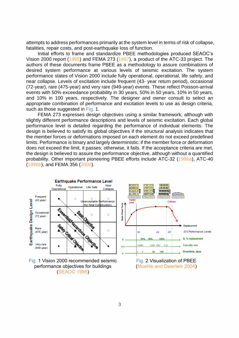
Initial efforts to frame and standardize PBEE methodologies produced SEAOC’s Vision 2000 report (1995) and FEMA 273 (1997), a product of the ATC-33 project. The authors of these documents frame PBEE as a methodology to assure combinations of desired system performance at various levels of seismic excitation. The system performance states of Vision 2000 include fully operational, operational, life safety, and near collapse. Levels of excitation include frequent (43- year return period), occasional (72-year), rare (475-year) and very rare (949-year) events. These reflect Poisson-arrival events with 50% exceedance probability in 30 years, 50% in 50 years, 10% in 50 years, and 10% in 100 years, respectively. The designer and owner consult to select an appropriate combination of performance and excitation levels to use as design criteria, such as those suggested in Fig. 1.

FEMA 273 expresses design objectives using a similar framework, although with slightly different performance descriptions and levels of seismic excitation. Each global performance level is detailed regarding the performance of individual elements. The design is believed to satisfy its global objectives if the structural analysis indicates that the member forces or deformations imposed on each element do not exceed predefined limits. Performance is binary and largely deterministic: if the member force or deformation does not exceed the limit, it passes; otherwise, it fails. If the acceptance criteria are met, the design is believed to assure the performance objective, although without a quantified probability. Other important pioneering PBEE efforts include ATC-32 (1996a), ATC-40 (1996b), and FEMA 356 (2000).

Fig. 1 Vision 2000 recommended seismic performance objectives for buildings

(SEAOC 1995)

Fig. 2 Visualization of PBEE (Moehle and Deierlein 2004)

4

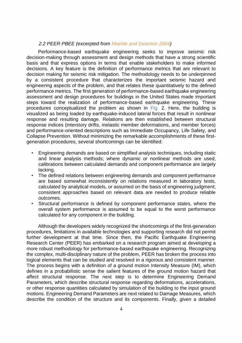
2.2 PEER PBEE (excerpted from Moehle and Deierlein 2004)

Performance-based earthquake engineering seeks to improve seismic risk decision-making through assessment and design methods that have a strong scientific basis and that express options in terms that enable stakeholders to make informed decisions. A key feature is the definition of performance metrics that are relevant to decision making for seismic risk mitigation. The methodology needs to be underpinned by a consistent procedure that characterizes the important seismic hazard and engineering aspects of the problem, and that relates these quantitatively to the defined performance metrics. The first generation of performance-based earthquake engineering assessment and design procedures for buildings in the United States made important steps toward the realization of performance-based earthquake engineering. These procedures conceptualized the problem as shown in Fig. 2. Here, the building is visualized as being loaded by earthquake-induced lateral forces that result in nonlinear response and resulting damage. Relations are then established between structural response indices (interstory drifts, inelastic member deformations, and member forces) and performance-oriented descriptions such as Immediate Occupancy, Life Safety, and Collapse Prevention. Without minimizing the remarkable accomplishments of these first-generation procedures, several shortcomings can be identified:

• Engineering demands are based on simplified analysis techniques, including static and linear analysis methods; where dynamic or nonlinear methods are used, calibrations between calculated demands and component performance are largely lacking.

• The defined relations between engineering demands and component performance are based somewhat inconsistently on relations measured in laboratory tests, calculated by analytical models, or assumed on the basis of engineering judgment; consistent approaches based on relevant data are needed to produce reliable outcomes.

• Structural performance is defined by component performance states, where the overall system performance is assumed to be equal to the worst performance calculated for any component in the building.

Although the developers widely recognized the shortcomings of the first-generation

procedures, limitations in available technologies and supporting research did not permit further development at that time. Since then, the Pacific Earthquake Engineering Research Center (PEER) has embarked on a research program aimed at developing a more robust methodology for performance-based earthquake engineering. Recognizing the complex, multi-disciplinary nature of the problem, PEER has broken the process into logical elements that can be studied and resolved in a rigorous and consistent manner. The process begins with a definition of a ground motion Intensity Measure (IM), which defines in a probabilistic sense the salient features of the ground motion hazard that affect structural response. The next step is to determine Engineering Demand Parameters, which describe structural response regarding deformations, accelerations, or other response quantities calculated by simulation of the building to the input ground motions. Engineering Demand Parameters are next related to Damage Measures, which describe the condition of the structure and its components. Finally, given a detailed

5

probabilistic description of damage, the process culminates with calculations of Decision Variables, which translate the damage into quantities that enter into risk management decisions. Consistent with current understanding of the needs of decision-makers, the decision variables have been defined in terms of quantities such as repair costs, downtime, and casualty rates (Fig. 2). Underlying the methodology is a consistent framework for representing the inherent uncertainties in earthquake performance assessment.

While full realization of the methodology in professional practice is still years away, important advances are being made through research in PEER. Some specific highlights are presented in the following text.

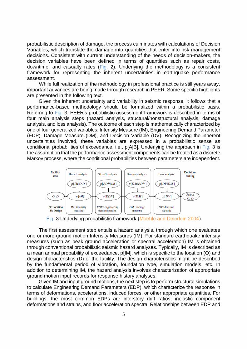
Given the inherent uncertainty and variability in seismic response, it follows that a performance-based methodology should be formalized within a probabilistic basis. Referring to Fig. 3, PEER’s probabilistic assessment framework is described in terms of four main analysis steps (hazard analysis, structural/nonstructural analysis, damage analysis, and loss analysis). The outcome of each step is mathematically characterized by one of four generalized variables: Intensity Measure (IM), Engineering Demand Parameter (EDP), Damage Measure (DM), and Decision Variable (DV). Recognizing the inherent uncertainties involved, these variables are expressed in a probabilistic sense as conditional probabilities of exceedance, i.e., p[A|B]. Underlying the approach in Fig. 3 is the assumption that the performance assessment components can be treated as a discrete Markov process, where the conditional probabilities between parameters are independent.

Fig. 3 Underlying probabilistic framework (Moehle and Deierlein 2004)

The first assessment step entails a hazard analysis, through which one evaluates

one or more ground motion Intensity Measures (IM). For standard earthquake intensity measures (such as peak ground acceleration or spectral acceleration) IM is obtained through conventional probabilistic seismic hazard analyses. Typically, IM is described as a mean annual probability of exceedance, p[IM], which is specific to the location (O) and design characteristics (D) of the facility. The design characteristics might be described by the fundamental period of vibration, foundation type, simulation models, etc. In addition to determining IM, the hazard analysis involves characterization of appropriate ground motion input records for response history analyses.

Given IM and input ground motions, the next step is to perform structural simulations to calculate Engineering Demand Parameters (EDP), which characterize the response in terms of deformations, accelerations, induced forces, or other appropriate quantities. For buildings, the most common EDPs are interstory drift ratios, inelastic component deformations and strains, and floor acceleration spectra. Relationships between EDP and

6

IM are typically obtained through inelastic simulations, which rely on models and simulation tools in areas of structural engineering, geotechnical engineering, SSFI (soil-structure-foundation-interaction), and non-structural component and system response.

The next step in the process is to perform a damage analysis, which relates the EDPs to Damage Measures, DM, which in turn describes the physical damage to a facility. The DMs include descriptions of damage to structural elements, non-structural elements, and contents, in order to quantify the necessary repairs along with functional or life safety implications of the damage (e.g., falling hazards, the release of hazardous substances, etc.). These conditional probability relationships, p(DM|EDP), can then be integrated with the EDP probability, p(EDP), to give the mean annual probability of exceedance for the DM, i.e., p(DM).

The final step in the assessment is to calculate Decision Variables, DV, in terms that are meaningful for decision makers. Generally speaking, the DVs relate to one of the three decision metrics discussed above with regard to Fig. 2, i.e., direct dollar losses, downtime (or restoration time), and casualties. In a similar manner as done for the other variables, the DVs are determined by integrating the conditional probabilities of DV given DM, p(DV|DM), with the mean annual DM probability of exceedance, p(DM).

The methodology just described and shown in Fig. 3 is an effective integrating construct for both the performance-based earthquake engineering methodology. The methodology can be expressed in terms of a triple integral based on the total probability theorem, as stated in Eq. 1.

ν(𝐷𝑉) =∭𝐺⟨𝐷𝑉|𝐷𝑀⟩|𝑑𝐺⟨𝐷𝑀|𝐸𝐷𝑃⟩|𝑑𝐺⟨𝐸𝐷𝑃|𝐼𝑀⟩|𝑑𝜆(𝐼𝑀) (1)

Though this equation form of the methodology might be construed as a minimalist

representation of a very complex problem, it nonetheless serves a useful function by providing researchers with a clear illustration of where their discipline-specific contribution fits into the broader scheme of performance-based earthquake engineering and how their research results need to be presented. The equation also emphasizes the inherent uncertainties in all phases of the problem and provides a consistent format for sharing and integrating data and models developed by researchers in the various disciplines.

The proposed methodology is intended to serve two related purposes. The first of these is as a performance engine to be applied in full detail to the seismic performance assessment of a facility. As illustrated in Fig. 2, the application would result in a comprehensive statement of the probabilities of various losses (in terms of dollars, downtime, and casualties) for events or time frames of interest to the owner or decision maker for that facility. Though illustrated in an apparent static loading domain in Fig. 2, this is for illustrative purposes only; the intent is to apply the methodology using a fully nonlinear dynamic analysis.

It leads to the second intended purpose of the methodology. Presuming it can be used to provide reliable results for a complete facility analysis, the methodology then can be used as a means of calibrating simplified procedures that might be used for the advancement of future building codes. It is in this application that the methodology is likely to have its largest potential impact.

7

3. SEISMIC HAZARD IN MODERATE-SEISMICITY REGIONS 3.1 Definition of moderate seismicity region (excerpted from Scholz 2002)

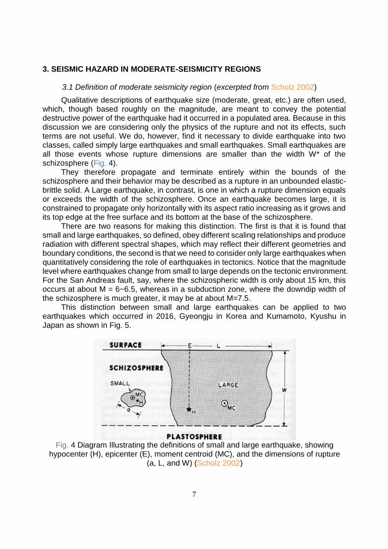
Qualitative descriptions of earthquake size (moderate, great, etc.) are often used, which, though based roughly on the magnitude, are meant to convey the potential destructive power of the earthquake had it occurred in a populated area. Because in this discussion we are considering only the physics of the rupture and not its effects, such terms are not useful. We do, however, find it necessary to divide earthquake into two classes, called simply large earthquakes and small earthquakes. Small earthquakes are all those events whose rupture dimensions are smaller than the width W* of the schizosphere (Fig. 4).

They therefore propagate and terminate entirely within the bounds of the schizosphere and their behavior may be described as a rupture in an unbounded elastic-brittle solid. A Large earthquake, in contrast, is one in which a rupture dimension equals or exceeds the width of the schizosphere. Once an earthquake becomes large, it is constrained to propagate only horizontally with its aspect ratio increasing as it grows and its top edge at the free surface and its bottom at the base of the schizosphere.

There are two reasons for making this distinction. The first is that it is found that small and large earthquakes, so defined, obey different scaling relationships and produce radiation with different spectral shapes, which may reflect their different geometries and boundary conditions, the second is that we need to consider only large earthquakes when quantitatively considering the role of earthquakes in tectonics. Notice that the magnitude level where earthquakes change from small to large depends on the tectonic environment. For the San Andreas fault, say, where the schizospheric width is only about 15 km, this occurs at about M = 6~6.5, whereas in a subduction zone, where the downdip width of the schizosphere is much greater, it may be at about M=7.5.

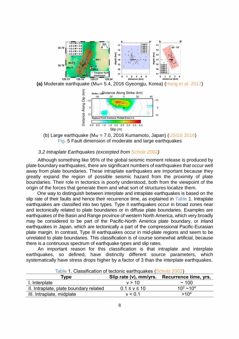
This distinction between small and large earthquakes can be applied to two earthquakes which occurred in 2016, Gyeongju in Korea and Kumamoto, Kyushu in Japan as shown in Fig. 5.

Fig. 4 Diagram Illustrating the definitions of small and large earthquake, showing

hypocenter (H), epicenter (E), moment centroid (MC), and the dimensions of rupture (a, L, and W) (Scholz 2002)

8

(a) Moderate earthquake (MW= 5.4, 2016 Gyeongju, Korea) (Hong et al. 2017)

(b) Large earthquake (MW = 7.0, 2016 Kumamoto, Japan) (USGS 2016)

Fig. 5 Fault dimension of moderate and large earthquakes

3.2 Intraplate Earthquakes (excerpted from Scholz 2002)

Although something like 95% of the global seismic moment release is produced by plate boundary earthquakes, there are significant numbers of earthquakes that occur well away from plate boundaries. These intraplate earthquakes are important because they greatly expand the region of possible seismic hazard from the proximity of plate boundaries. Their role in tectonics is poorly understood, both from the viewpoint of the origin of the forces that generate them and what sort of structures localize them.

One way to distinguish between interplate and intraplate earthquakes is based on the slip rate of their faults and hence their recurrence time, as explained in Table 1. Intraplate earthquakes are classified into two types. Type II earthquakes occur in broad zones near and tectonically related to plate boundaries or in diffuse plate boundaries. Examples are earthquakes of the Basin and Range province of western North America, which very broadly may be considered to be part of the Pacific-North America plate boundary, or inland earthquakes in Japan, which are tectonically a part of the compressional Pacific-Eurasian plate margin. In contrast, Type III earthquakes occur in mid-plate regions and seem to be unrelated to plate boundaries. This classification is of course somewhat artificial, because there is a continuous spectrum of earthquake types and slip rates.

An important reason for this classification is that intraplate and interplate earthquakes, so defined, have distinctly different source parameters, which systematically have stress drops higher by a factor of 3 than the interplate earthquakes.

Table 1. Classification of tectonic earthquakes (Scholz 2002)

Type Slip rate (v), mm/yrs. Recurrence time, yrs.

I. Interplate ν > 10 ~ 100

II. Intraplate, plate boundary related 0.1 ≤ ν ≤ 10 102 ~104

III. Intraplate, midplate ν < 0.1 >104

9

3.3 Characteristics of the seismic hazard in moderate seismicity regions

Either very infrequent major earthquakes or infrequent moderate earthquakes are known to have occurred in east northern America (ENA). In either case, the more recent seismic activity is minor. An example might be a region with a single recorded occurrence of a magnitude 7 or larger earthquake, and no damaging earthquake since (e.g., Memphis, Charleston, or Boston) or a string of earthquakes of magnitude 5 to 5.5 and sufficient geologic evidence to imply the possibility of a rare larger event. (Nordenson and Bell 2000)

• The localities are not expecting nor are generally prepared for an earthquake, and the buildings are, for the most part, not earthquake resistant.

• Typically, these regions are located away from tectonic plate boundaries, and major faults, and so the source of earthquakes is less well understood and hazards assessments are more difficult.

• The ground shaking caused by earthquakes diminishes, or “attenuates,” much less with increasing distance from the earthquake. That means that for a given magnitude the “felt area” and extent of damage is much greater in most moderate seismic regions than in high seismic regions.

• There are few active faults, for which there is an average historic slip rate of 1 mm per year or more and evidence of seismic activity within Holocene times (the past 11,000 years), and all the faults are hidden faults.

• Charleston earthquake (1886) was an exceptionally large magnitude earthquake without any surface rupture in Fig. 6. The shaking effects of the 31 August 1886 Charleston, South Carolina, earthquake indicate that it was a major shock. Moment magnitude estimates range from Mw 6.9 (Bakun and Hopper 2004) to Mw 7.3 (Johnston 1996). The fault movement that was the cause of the 1886 South Carolina earthquake did not rupture the Earth's surface, but rather was confined to its interior. Therefore, an important piece of direct field evidence, the direction of the trend (termed by geologists the "strike") of the fault surface was not provided for this earthquake nor was the direction of movement on the fault; that is, vertical, horizontal, or some combination.

(a) Reported intensities (Johnston 1996) (b) Damage and collapse of buildings

Fig. 6 The 1886 Charleston earthquake

10

3.4 Background seismic hazard maps in moderate seismicity regions

CENA in U.S.A. (excerpted from Frankel 1995)

Fig. 7 diagrams the four-model method used for the hazard map in Central and Eastern (CENA) U.S.A. Three alternative models of hazard are used for this magnitude range (Fig. 7 left). Model 1 is based on spatially-smoothed a-values derived from the magnitude 3 and larger earthquakes since 1924. Here a is the activity level in the Gutenberg-Richter equation log N = a-bM, where N is the number of events with magnitudes greater or equal to M. In this model, the magnitude 3 and greater events are assumed to illuminate areas of faulting which can produce destructive events.

Fig. 7 Chart of four models to make seismic hazard maps in the CENA in U.S.A.

(Frankel 1995) The areas of large ground motions in Fig. 8(a) simply indicate areas with larger

numbers of magnitude 3 and larger events since 1924. This map does not contain the hazard from events with magnitudes larger than 7.0, so it underestimates the probabilistic ground motions for New Madrid and Charleston.

A trial map of probabilistic ground motions for model 3 (Fig. 7) is shown in Fig. 8(b). The 25 cm/sec 2 contour line basically follows the boundary of the source zone. The area within the 25 cm/sec2 contour (Fig. 8(b)) has a probabilistic ground motion of about 30 cm/ sec2 (3% g), for 10% PE in 50 years.

(a) model 1 (b) model 3

Fig. 8 Trial ground-motion map for models 1 and 3, 10% probability of exceedance in 50years (Values are peak ground acceleration in cm/sec2) (Frankel 1995)

11

A simple background seismic hazard in Korean Peninsula

PSHA is composed of 4 steps as shown in Fig. 9. The first step is the identification of all the sources of earthquakes. Second is the statistical representation of the relation between the magnitude of the earthquake and its frequencies by the Gutenberg-Richter recurrence law. The third is the establishment of the attenuation law between the ground motion parameters and the rupture or epicentral distance where the median and standard deviation of ground motion parameters are to be obtained. Finally, the fourth step is to derive the hazard curve represented by the relation between the hazard parameter and the probability of exceedance of the specific parameter value.

Fig. 9 Four steps of a probabilistic seismic hazard analysis (Kramer 1996)

Uniform background zone in Fig. 8(b) assumes that the probability of occurrence of

the earthquake (Fig. 10) is uniform all over the region, so the number of occurrence for each level of the earthquake is distributed uniformly as shown in Table 2.

Fig. 10 Probability of occurrence of earthquake

Table 2. Number of M 5 intraplate earthquake events on land in a 50 years period (Lam 2014) Country Land Area

(km) N(M5) in 50 years

[Recorded Number] N(M5) in 50 years

[Recorded Number Normalized to 1,000,000 km2]

Australia 7,692,024 45 6

Brazil 8,515,767 33 4

Eastern US 2,291,043 13 5 6

Eastern & Central China 1,550,974 14 9

France 674,843 4 6

Southern India 635,780 3 5

Germany 357,021 1 3

British Isles 315,134 3 9 10

Peninsular Malaysia 131,598 <1 <1

Korean Peninsula 223,348 3 13

Total = 22,387,532 = 120 Average = 5

Site

R

=Area Area

RiRi-1

• Rmax =200 km

• Area(Total)

=125,664 km2

12

The earthquake recurrence relationship (Fig. 11) assuming a doubly-truncated exponential function can be expressed as follows:

𝜆𝑚 = 𝜈exp[−𝛽(𝑚−𝑚0)] −exp[−𝛽(𝑚𝑚𝑎𝑥−𝑚0)]

1−exp[−𝛽(𝑚𝑚𝑎𝑥−𝑚0)] (2)

𝑚0 ≤ 𝑚 ≤ 𝑚𝑚𝑎𝑥, 𝑚0 = 4

𝜈 = exp(𝛼 − 𝛽𝑚0) 𝛼 = 2.303a 𝛽 = 2.303𝑏

Fig. 11 Earthquake recurrence relationship where 𝜆𝑚 is the number of earthquakes with magnitude greater than M, occurring in a fixed time interval and within the circular source area of radius Rmax. ν is the total number of earthquakes with magnitude greater than Mmin, occurring in a fixed time interval and within the circular source area. β=2.3b, in which b is the slope of the Gutenberg-Richter relationship. The corresponding probability density function is defined as follows:

𝑓(𝑀) =𝛽 exp[−𝛽(𝑀 −𝑀𝑚𝑖𝑛)]

1 − exp[−𝛽(𝑀𝑚𝑎𝑥 −𝑀𝑚𝑖𝑛)] (3)

The probability distribution of PHA in Korea is assumed to be same as that given by GMPE of Boore (2008) in Fig. 12. For each combination of epicentral distance, magnitude, and PGA, the probability of exceedance (PGA ≥ y*) can be obtained using Eq. (4).

P[𝑃𝐺𝐴 > 𝑦∗|𝑚, 𝑟] = 1 − 𝐹𝑌 (ln𝑦∗=ln𝑃𝐺𝐴

𝜎ln𝑃𝐺𝐴) (4)

Fig. 12 Relationship between epicentral distance and PGA

0.00001

0.0001

0.001

0.01

0.1

1

4 5 6 7 8

λm

Magnitude, m

Constant seismicity rate

mmax 6 6.5 7 8

0

0.05

0.1

0.15

0.2

0.25

0.3

0.35

0.4

0 50 100 150 200

PG

A (

g)

Epicentral distance (km)

Attenuation relation (Boore 2008)

m = 6.25

Mean =

±1σ = ±0.5

13

For every combination of M and R, seismic intensities are predicted by employing suitable ground motion prediction equations (GMPEs). Finally, the total seismic hazard of the site encompassing all the considered M-R combinations can be computed using the conventional Cornell-McGuire approach (Cornell 1968, McGuire 1976) which is represented by the following integral:

𝜆𝑦∗ = 𝜈∑∑𝑃[𝑌 > 𝑦∗|𝑚𝑗 , 𝑟𝑘] 𝑃[𝑚𝑗] 𝑃[𝑟𝑘]

𝑁𝑅

𝑘=1

𝑁𝑀

𝑗=1

(5)

The probability of exceedance, or, the annual frequency of PGA ≥ y* is shown in

Fig. 13, where PGA’s corresponding to the probability of exceedance 10% and 2% in 50 years are 0.0253 and 0.0541g, respectively. The value of 0.025g for the probability of 10% in 50 years is similar to the value of 2.5%g in the uniform background zone in Fig. 8(b). these PGA’s are compared with the effective PGA in KBC 2016 (Table 4) where PGA’s in KBC 2016 are about four times larger than those based on uniform background zone in Korean Peninsula.

Fig. 13 Mean annual rate of exceedance of PGA for Korean Peninsula

Table 3. Comparison between Effective PGA in KBC 2016 and Background Hazard

Return periods (year) KBC 2016 Background Hazard

500 0.11g 0.0253g

2500 0.22g 0.0541g

The disaggregation for PGA 0.05g and PGA 0.11g (Fig. 14) are shown as

histograms on the epicentral distance and the magnitude. It can be found in this figure that most of the contribution comes from within the distance less than 50 km and from the magnitude ranging from M 4.5 to 6.5. In moderate seismicity regions such as ENA and Korean Peninsula, the hazard derived from uniform background zone serve as the lower bound for the probabilistic seismic hazard map.

(0.11g, 0.0000549 )

RP. 18200 yrs.

(0.05g, 0.000490 )

RP. 2043 yrs.

(0.0541g, 0.000404)

RP. 2476 yrs.

(0.0253g, 0.00212)

RP. 475 yrs

1E-09

1E-08

0.0000001

0.000001

0.00001

0.0001

0.001

0.01

0.1

0 0.05 0.1 0.15 0.2

Mea

n a

nnual

rat

e o

f ex

ceed

ance

of

PG

A

Peak Ground Acceleration (PGA, g)

Seismic Hazard Curve

(지진재해도곡선)

14

(a) 0.05 g (b) 0.11 g

Fig. 14 Disaggregation for PGA: 0.05g and 0.11g 3.5 Seismicity and seismic hazard map in Korean Peninsula

Historical earthquakes were recorded in various historical sources including Samgooksagi, Koryosa, and Choseon-wangjosillog, which were listed in various studies (e.g., Wada, 1912; Lee and Yang, 2006). The seismic intensities and source information of historical events during 2–1904 A.D. are collected from Lee and Yang (2006). The number of earthquakes during the period of the Three Kingdoms is 56, earthquakes during the period of the Unified Silla is 33, earthquakes during the period of the Koryo dynasty is 158, and earthquakes during the period of the Choseon dynasty is 1938 (Fig. 15(a)).

The historical earthquake records during the Choseon dynasty comprise about 89% of the total historical earthquake records. Large-size events with seismic intensities of VIII to IX are recorded mostly in the periods before the Choseon dynasty. On the contrary, earthquakes with seismic intensities greater than IV were recorded well during the Choseon dynasty (Fig. 15).

Fig. 15 (a) Temporal distribution and seismic intensities of historical earthquake

during 2-1904 A.D.; (b) Histogram for the numbers of records for every 50-year period; and (c) Gutenberg-Richter recurrence law between magnitude and frequency

(Houng and Hong 2013) From these data, Gutenberg-Richter recurrence law between magnitude and

frequency is shown in Fig. 15(c). However, the maximum magnitude is estimated to be 7.45±0.04, which appears to be an excessive overestimation due to the fact that no active fault having surface rupture regarding this maximum event could be identified, and the range of the region of the damage and casualties were not nationwide.

4.25

5.25

6.25

0.00E+00

1.00E-05

2.00E-05

3.00E-05

4.00E-05

5.00E-05

7 16 25 35 45 55 65 75 85 95 105 115

Mag

nit

ud

e

λm

Distance (km)

Annaual rate of exceedance of a PGA 0.05g

4.0~4.54.5~5.0

5.0~5.55.5~6.0

6.0~6.5

4.25

5.25

6.25

0.00E+00

2.00E-06

4.00E-06

6.00E-06

8.00E-06

1.00E-05

7 16 25 35 45 55 65 75 85 95 105 115

Mag

nit

ud

e

λm

Distance (km)

Annaual rate of exceedance of a PGA 0.11g

4.0~4.54.5~5.0

5.0~5.55.5~6.0

6.0~6.5

(c)

15

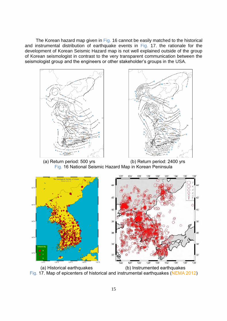
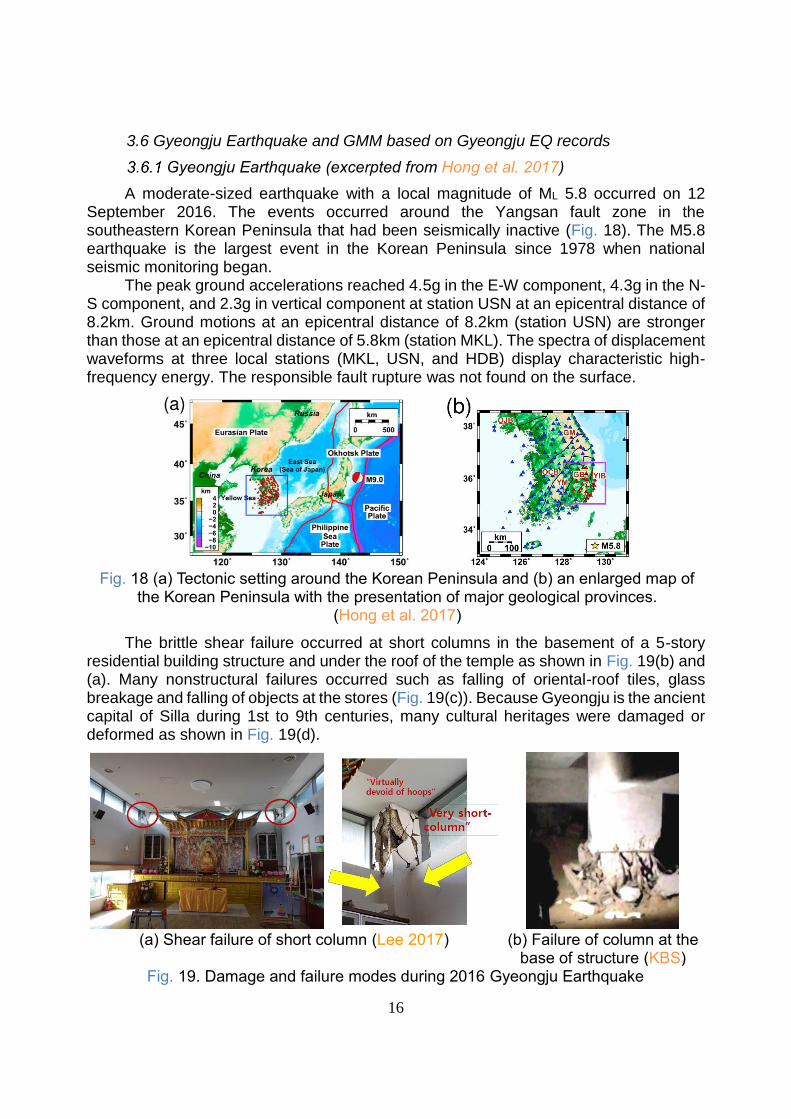
The Korean hazard map given in Fig. 16 cannot be easily matched to the historical and instrumental distribution of earthquake events in Fig. 17. the rationale for the development of Korean Seismic Hazard map is not well explained outside of the group of Korean seismologist in contrast to the very transparent communication between the seismologist group and the engineers or other stakeholder’s groups in the USA.

(a) Return period: 500 yrs (b) Return period: 2400 yrs

Fig. 16 National Seismic Hazard Map in Korean Peninsula

(a) Historical earthquakes (b) Instrumented earthquakes

Fig. 17. Map of epicenters of historical and instrumental earthquakes (NEMA 2012)

16

3.6 Gyeongju Earthquake and GMM based on Gyeongju EQ records

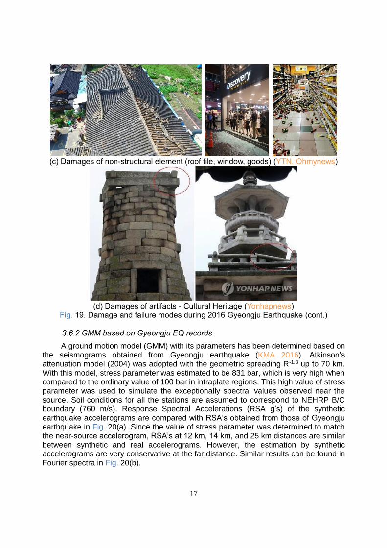
Gyeongju Earthquake (excerpted from Hong et al. 2017)

A moderate-sized earthquake with a local magnitude of ML 5.8 occurred on 12 September 2016. The events occurred around the Yangsan fault zone in the southeastern Korean Peninsula that had been seismically inactive (Fig. 18). The M5.8 earthquake is the largest event in the Korean Peninsula since 1978 when national seismic monitoring began.

The peak ground accelerations reached 4.5g in the E-W component, 4.3g in the N-S component, and 2.3g in vertical component at station USN at an epicentral distance of 8.2km. Ground motions at an epicentral distance of 8.2km (station USN) are stronger than those at an epicentral distance of 5.8km (station MKL). The spectra of displacement waveforms at three local stations (MKL, USN, and HDB) display characteristic high-frequency energy. The responsible fault rupture was not found on the surface.

Fig. 18 (a) Tectonic setting around the Korean Peninsula and (b) an enlarged map of

the Korean Peninsula with the presentation of major geological provinces. (Hong et al. 2017)

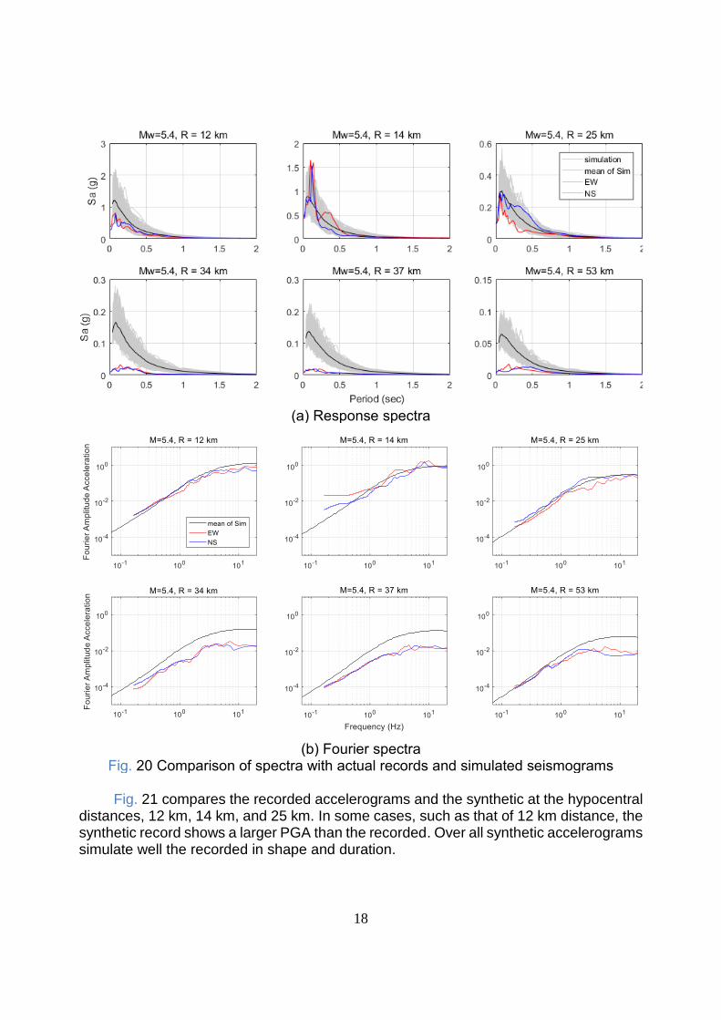
The brittle shear failure occurred at short columns in the basement of a 5-story residential building structure and under the roof of the temple as shown in Fig. 19(b) and (a). Many nonstructural failures occurred such as falling of oriental-roof tiles, glass breakage and falling of objects at the stores (Fig. 19(c)). Because Gyeongju is the ancient capital of Silla during 1st to 9th centuries, many cultural heritages were damaged or deformed as shown in Fig. 19(d).

(a) Shear failure of short column (Lee 2017) (b) Failure of column at the

base of structure (KBS) Fig. 19. Damage and failure modes during 2016 Gyeongju Earthquake

17

(c) Damages of non-structural element (roof tile, window, goods) (YTN, Ohmynews)

(d) Damages of artifacts - Cultural Heritage (Yonhapnews)

Fig. 19. Damage and failure modes during 2016 Gyeongju Earthquake (cont.)

GMM based on Gyeongju EQ records

A ground motion model (GMM) with its parameters has been determined based on the seismograms obtained from Gyeongju earthquake (KMA 2016). Atkinson’s attenuation model (2004) was adopted with the geometric spreading R-1.3 up to 70 km. With this model, stress parameter was estimated to be 831 bar, which is very high when compared to the ordinary value of 100 bar in intraplate regions. This high value of stress parameter was used to simulate the exceptionally spectral values observed near the source. Soil conditions for all the stations are assumed to correspond to NEHRP B/C boundary (760 m/s). Response Spectral Accelerations (RSA g’s) of the synthetic earthquake accelerograms are compared with RSA’s obtained from those of Gyeongju earthquake in Fig. 20(a). Since the value of stress parameter was determined to match the near-source accelerogram, RSA’s at 12 km, 14 km, and 25 km distances are similar between synthetic and real accelerograms. However, the estimation by synthetic accelerograms are very conservative at the far distance. Similar results can be found in Fourier spectra in Fig. 20(b).

18

(a) Response spectra

(b) Fourier spectra

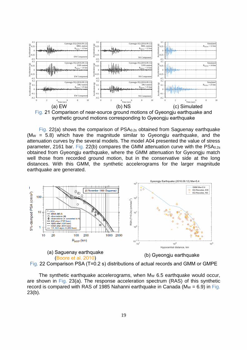
Fig. 20 Comparison of spectra with actual records and simulated seismograms Fig. 21 compares the recorded accelerograms and the synthetic at the hypocentral

distances, 12 km, 14 km, and 25 km. In some cases, such as that of 12 km distance, the synthetic record shows a larger PGA than the recorded. Over all synthetic accelerograms simulate well the recorded in shape and duration.

19

(a) EW (b) NS (c) Simulated

Fig. 21 Comparison of near-source ground motions of Gyeongju earthquake and synthetic ground motions corresponding to Gyeongju earthquake

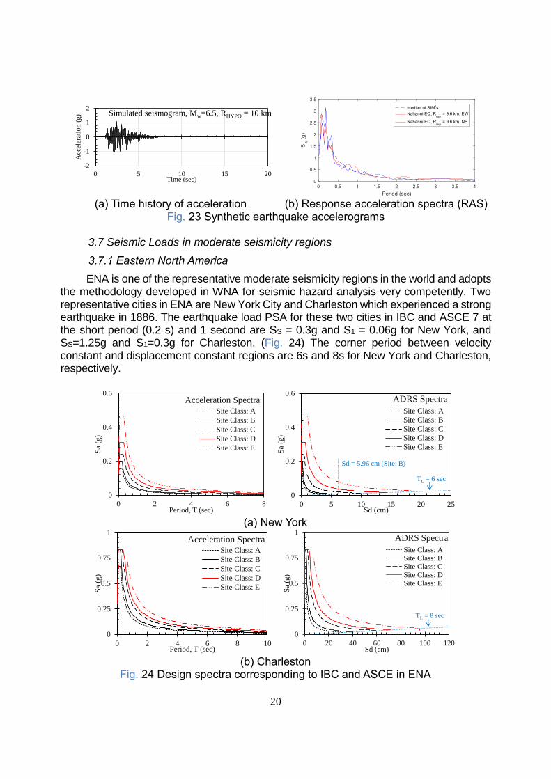
Fig. 22(a) shows the comparison of PSA0.2s obtained from Saguenay earthquake

(MW = 5.8) which have the magnitude similar to Gyeongju earthquake, and the attenuation curves by the several models. The model A04 presented the value of stress parameter, 2161 bar. Fig. 22(b) compares the GMM attenuation curve with the PSA0.2s obtained from Gyeongju earthquake, where the GMM attenuation for Gyeongju match well those from recorded ground motion, but in the conservative side at the long distances. With this GMM, the synthetic accelerograms for the larger magnitude earthquake are generated.

(a) Saguenay earthquake (Boore et al. 2010)

(b) Gyeongju earthquake

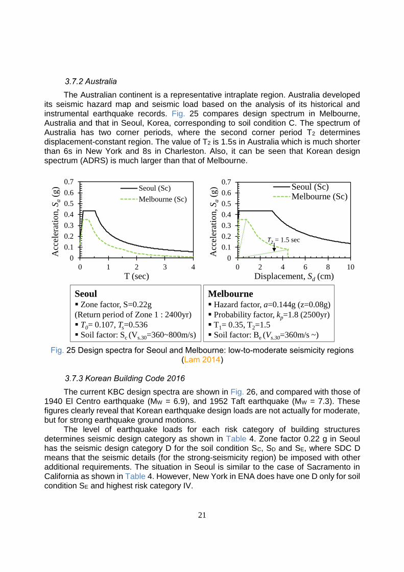
Fig. 22 Comparison PSA (T=0.2 s) distributions of actual records and GMM or GMPE The synthetic earthquake accelerograms, when MW 6.5 earthquake would occur,

are shown in Fig. 23(a). The response acceleration spectrum (RAS) of this synthetic record is compared with RAS of 1985 Nahanni earthquake in Canada (MW = 6.9) in Fig. 23(b).

-0.5

-0.25

0

0.25

0.5

0 2 4 6 8 10

Acc

eler

atio

n (

g)

Time (sec)

Gyeongju EQ (2016.09.12)

MKL station

RHYPO = 12 km

EW Component

-0.5

-0.25

0

0.25

0.5

0 2 4 6 8 10

Acc

eler

atio

n (

g)

Time (sec)

Gyeongju EQ (2016.09.12)

USN station

RHYPO = 14 km

EW Component

-0.2

-0.1

0

0.1

0.2

0 2 4 6 8 10

Acc

eler

atio

n (

g)

Time (sec)

Gyeongju EQ (2016.09.12)

DKJ station

RHYPO = 25 km

EW Component

-0.5

-0.25

0

0.25

0.5

0 2 4 6 8 10

Acc

eler

atio

n (

g)

Time (sec)

Gyeongju EQ (2016.09.12)

MKL station

RHYPO = 12 km

NS Component

-0.5

-0.25

0

0.25

0.5

0 2 4 6 8 10

Acc

eler

atio

n (

g)

Time (sec)

Gyeongju EQ (2016.09.12)

USN station

RHYPO = 14 km

NS Component

-0.2

-0.1

0

0.1

0.2

0 2 4 6 8 10

Acc

eler

atio

n (

g)

Time (sec)

Gyeongju EQ (2016.09.12)

DKJ station

RHYPO = 25 km

NS Component

-0.5

-0.25

0

0.25

0.5

0 2 4 6 8 10

Acc

eler

atio

n (

g)

Time (sec)

Simulated

RHYPO = 12 km

-0.5

-0.25

0

0.25

0.5

0 2 4 6 8 10

Acc

eler

atio

n (

g)

Time (sec)

Simulated

RHYPO = 14 km

-0.2

-0.1

0

0.1

0.2

0 2 4 6 8 10

Acc

eler

atio

n (

g)

Time (sec)

Simulated

RHYPO = 25 km

20

(a) Time history of acceleration (b) Response acceleration spectra (RAS)

Fig. 23 Synthetic earthquake accelerograms 3.7 Seismic Loads in moderate seismicity regions

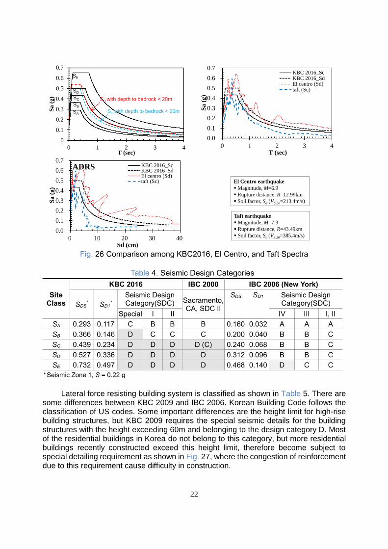
Eastern North America

ENA is one of the representative moderate seismicity regions in the world and adopts the methodology developed in WNA for seismic hazard analysis very competently. Two representative cities in ENA are New York City and Charleston which experienced a strong earthquake in 1886. The earthquake load PSA for these two cities in IBC and ASCE 7 at the short period (0.2 s) and 1 second are SS = 0.3g and S1 = 0.06g for New York, and SS=1.25g and S1=0.3g for Charleston. (Fig. 24) The corner period between velocity constant and displacement constant regions are 6s and 8s for New York and Charleston, respectively.

(a) New York

(b) Charleston

Fig. 24 Design spectra corresponding to IBC and ASCE in ENA

-2

-1

0

1

2

0 5 10 15 20

Acc

eler

atio

n (

g)

Time (sec)

Simulated seismogram, Mw=6.5, RHYPO = 10 km

0

0.2

0.4

0.6

0 2 4 6 8

Sa

(g)

Period, T (sec)

Acceleration Spectra

Site Class: A

Site Class: B

Site Class: C

Site Class: D

Site Class: E

0

0.2

0.4

0.6

0 5 10 15 20 25

Sa

(g)

Sd (cm)

ADRS Spectra

Site Class: A

Site Class: B

Site Class: C

Site Class: D

Site Class: E

TL = 6 sec

Sd = 5.96 cm (Site: B)

0

0.25

0.5

0.75

1

0 2 4 6 8 10

Sa

(g)

Period, T (sec)

Acceleration SpectraSite Class: A

Site Class: B

Site Class: C

Site Class: D

Site Class: E

0

0.25

0.5

0.75

1

0 20 40 60 80 100 120

Sa

(g)

Sd (cm)

ADRS Spectra

Site Class: ASite Class: BSite Class: CSite Class: DSite Class: E

TL = 8 sec

21

Australia

The Australian continent is a representative intraplate region. Australia developed its seismic hazard map and seismic load based on the analysis of its historical and instrumental earthquake records. Fig. 25 compares design spectrum in Melbourne, Australia and that in Seoul, Korea, corresponding to soil condition C. The spectrum of Australia has two corner periods, where the second corner period T2 determines displacement-constant region. The value of T2 is 1.5s in Australia which is much shorter than 6s in New York and 8s in Charleston. Also, it can be seen that Korean design spectrum (ADRS) is much larger than that of Melbourne.

Fig. 25 Design spectra for Seoul and Melbourne: low-to-moderate seismicity regions

(Lam 2014)

Korean Building Code 2016

The current KBC design spectra are shown in Fig. 26, and compared with those of 1940 El Centro earthquake (MW = 6.9), and 1952 Taft earthquake (MW = 7.3). These figures clearly reveal that Korean earthquake design loads are not actually for moderate, but for strong earthquake ground motions.

The level of earthquake loads for each risk category of building structures determines seismic design category as shown in Table 4. Zone factor 0.22 g in Seoul has the seismic design category D for the soil condition SC, SD and SE, where SDC D means that the seismic details (for the strong-seismicity region) be imposed with other additional requirements. The situation in Seoul is similar to the case of Sacramento in California as shown in Table 4. However, New York in ENA does have one D only for soil condition SE and highest risk category IV.

0

0.1

0.2

0.3

0.4

0.5

0.6

0.7

0 1 2 3 4

Acc

eler

atio

n, S

a(g

)

T (sec)

Seoul (Sc)

Melbourne (Sc)

0

0.1

0.2

0.3

0.4

0.5

0.6

0.7

0 2 4 6 8 10

Acc

eler

atio

n, S

a(g

)

Displacement, Sd (cm)

Seoul (Sc)Melbourne (Sc)

T2 = 1.5 sec

0.0

0.1

0.2

0.3

0.4

0.5

0 5 10 15 20

Sa

(g

)

Sd (cm)

ADRSSeoul (Sc)

Melbourne (Sc)

0.0

0.1

0.2

0.3

0.4

0.5

0 1 2 3 4

Sa

(g

)

T (sec)

Design spectrum

Seoul (Sc)

Melbourne (Sc)

0

10

20

30

40

50

60

0 1 2 3 4

Sv

(cm

/s)

T (sec)

Design spectrum Seoul (Sc)

Melbourne (Sc)

Seoul▪ Zone factor, S=0.22g

(Return period of Zone 1 : 2400yr)

▪ T0= 0.107, Ts=0.536

▪ Soil factor: Sc (Vs.30=360~800m/s)

0

5

10

15

20

25

30

0 1 2 3 4

Sd

(cm

)

T (sec)

Design spectrum

Seoul (Sc)

Melbourne (Sc)

Melbourne▪ Hazard factor, a=0.144g (z=0.08g)

▪ Probability factor, kp=1.8 (2500yr)

▪ T1= 0.35, T2=1.5

▪ Soil factor: Be (Vs.30=360m/s ~)

22

Fig. 26 Comparison among KBC2016, El Centro, and Taft Spectra

Table 4. Seismic Design Categories

Site Class

KBC 2016 IBC 2000 IBC 2006 (New York)

SDS* SD1

*

Seismic Design Category(SDC) Sacramento,

CA, SDC II

SDS SD1 Seismic Design Category(SDC)

Special I II IV III I, II

SA 0.293 0.117 C B B B 0.160 0.032 A A A

SB 0.366 0.146 D C C C 0.200 0.040 B B C

SC 0.439 0.234 D D D D (C) 0.240 0.068 B B C

SD 0.527 0.336 D D D D 0.312 0.096 B B C

SE 0.732 0.497 D D D D 0.468 0.140 D C C

* Seismic Zone 1, S = 0.22 g

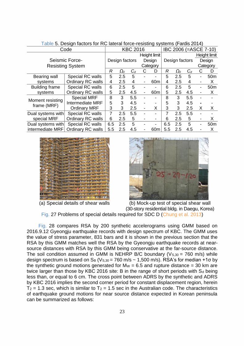
Lateral force resisting building system is classified as shown in Table 5. There are

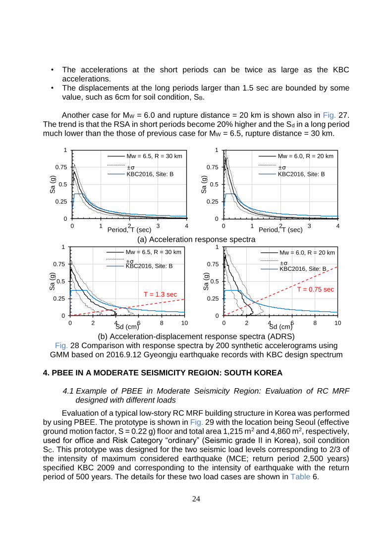
some differences between KBC 2009 and IBC 2006. Korean Building Code follows the classification of US codes. Some important differences are the height limit for high-rise building structures, but KBC 2009 requires the special seismic details for the building structures with the height exceeding 60m and belonging to the design category D. Most of the residential buildings in Korea do not belong to this category, but more residential buildings recently constructed exceed this height limit, therefore become subject to special detailing requirement as shown in Fig. 27, where the congestion of reinforcement due to this requirement cause difficulty in construction.

0

0.1

0.2

0.3

0.4

0.5

0.6

0.7

0 1 2 3 4

Sa (

g)

T (sec)

SE

SD

SC

SB

SA

SD with depth to bedrock < 20m

SC with depth to bedrock < 20m

0.0

0.1

0.2

0.3

0.4

0.5

0.6

0.7

0 1 2 3 4

Sa

(g

)

T (sec)

KBC 2016_ScKBC 2016_SdEl centro (Sd)taft (Sc)

0.0

0.1

0.2

0.3

0.4

0.5

0.6

0.7

0 10 20 30 40

Sa

(g

)

Sd (cm)

ADRS KBC 2016_ScKBC 2016_SdEl centro (Sd)taft (Sc) Taft earthquake

▪ Magnitude, M=7.3

▪ Rupture distance, R=43.49km

▪ Soil factor, Sc (VS.30=385.4m/s)

El Centro earthquake

▪ Magnitude, M=6.9

▪ Rupture distance, R=12.99km

▪ Soil factor, Sd (VS.30=213.4m/s)

0.0

0.2

0.4

0.6

0.8

0 1 2 3 4

Sa

(g

)

T (sec)

Design spectrum KBC 2009_Sc

KBC 2009_Sd

El centro (Sd)

taft (Sc)

0

20

40

60

80

100

120

0 1 2 3 4

Sv

(cm

/s)

T (sec)

Design spectrumKBC 2009_Sc

KBC 2009_Sd

El centro (Sd)

taft (Sc)

0

10

20

30

40

50

60

0 1 2 3 4

Sd

(cm

)

T (sec)

Design spectrum KBC 2009_Sc

KBC 2009_Sd

El centro (Sd)

taft (Sc)

0.0

0.2

0.4

0.6

0.8

0 10 20 30 40

Sa

(g

)

Sd (cm)

ADRS KBC 2009_Sc

KBC 2009_Sd

El centro (Sd)

taft (Sc)

Taft earthquake

▪ Magnitude, M=7.3

▪ Rupture distance, R=43.49km

▪ Soil factor, Sc (VS.30=385.4m/s)

El Centro earthquake

▪ Magnitude, M=6.9

▪ Rupture distance, R=12.99km

▪ Soil factor, Sd (VS.30=213.4m/s)

0.0

0.2

0.4

0.6

0.8

0 1 2 3 4

Sa

(g

)

T (sec)

Design spectrum KBC 2009_Sc

KBC 2009_Sd

El centro (Sd)

taft (Sc)

0

20

40

60

80

100

120

0 1 2 3 4

Sv

(cm

/s)

T (sec)

Design spectrumKBC 2009_Sc

KBC 2009_Sd

El centro (Sd)

taft (Sc)

0

10

20

30

40

50

60

0 1 2 3 4

Sd

(cm

)

T (sec)

Design spectrum KBC 2009_Sc

KBC 2009_Sd

El centro (Sd)

taft (Sc)

0.0

0.2

0.4

0.6

0.8

0 10 20 30 40

Sa

(g

)

Sd (cm)

ADRS KBC 2009_Sc

KBC 2009_Sd

El centro (Sd)

taft (Sc)

23

Table 5. Design factors for RC lateral force-resisting systems (Fardis 2014)

Code KBC 2016 IBC 2006 (=ASCE 7-10)

Seismic Force- Resisting System

Design factors

Height limit

Design factors

Height limit

Design Category

Design Category

R Ω0 Cd C D R Ω0 Cd C D

Bearing wall systems

Special RC walls 5 2.5 5 - - 5 2.5 5 - 50m Ordinary RC walls 4 2.5 4 - 60m 4 2.5 4 - X

Building frame systems

Special RC walls 6 2.5 5 - - 6 2.5 5 - 50m Ordinary RC walls 5 2.5 4.5 - 60m 5 2.5 4.5 - X

Moment resisting frame (MRF)

Special MRF 8 3 5.5 - - 8 3 5.5 - - Intermediate MRF 5 3 4.5 - - 5 3 4.5 - -

Ordinary MRF 3 3 2.5 - X 3 3 2.5 X X

Dual systems with special MRF

Special RC walls 7 2.5 5.5 - - 7 2.5 5.5 - - Ordinary RC walls 6 2.5 5 - - 6 2.5 5 - X

Dual systems with intermediate MRF

Special RC walls 6.5 2.5 5 - - 6.5 2.5 5 - 50m Ordinary RC walls 5.5 2.5 4.5 - 60m 5.5 2.5 4.5 - X

(a) Special details of shear walls (b) Mock-up test of special shear wall

(30-story residential bldg. in Daegu, Korea) Fig. 27 Problems of special details required for SDC D (Chung et al. 2013)

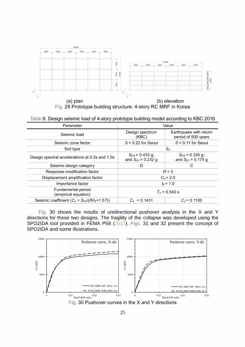
Fig. 28 compares RSA by 200 synthetic accelerograms using GMM based on

2016.9.12 Gyeongju earthquake records with design spectrum of KBC. The GMM uses the value of stress parameter, 831 bars and it is shown in the previous section that the RSA by this GMM matches well the RSA by the Gyeongju earthquake records at near-source distances with RSA by this GMM being conservative at the far-source distance. The soil condition assumed in GMM is NEHRP B/C boundary (VS,30 = 760 m/s) while design spectrum is based on SB (VS,30 = 760 m/s ~ 1,500 m/s). RSA’s for median +1σ by the synthetic ground motions generated for MW = 6.5 and rupture distance = 30 km are twice larger than those by KBC 2016 site: B in the range of short periods with Sd being less than, or equal to 6 cm. The cross point between ADRS by the synthetic and ADRS by KBC 2016 implies the second corner period for constant displacement region, herein T2 = 1.3 sec, which is similar to T2 = 1.5 sec in the Australian code. The characteristics of earthquake ground motions for near source distance expected in Korean peninsula can be summarized as follows:

24

• The accelerations at the short periods can be twice as large as the KBC accelerations.

• The displacements at the long periods larger than 1.5 sec are bounded by some value, such as 6cm for soil condition, SB. Another case for MW = 6.0 and rupture distance = 20 km is shown also in Fig. 27.

The trend is that the RSA in short periods become 20% higher and the Sd in a long period much lower than the those of previous case for MW = 6.5, rupture distance = 30 km.

(a) Acceleration response spectra

(b) Acceleration-displacement response spectra (ADRS)

Fig. 28 Comparison with response spectra by 200 synthetic accelerograms using GMM based on 2016.9.12 Gyeongju earthquake records with KBC design spectrum

4. PBEE IN A MODERATE SEISMICITY REGION: SOUTH KOREA

4.1 Example of PBEE in Moderate Seismicity Region: Evaluation of RC MRF

designed with different loads

Evaluation of a typical low-story RC MRF building structure in Korea was performed by using PBEE. The prototype is shown in Fig. 29 with the location being Seoul (effective ground motion factor, S = 0.22 g) floor and total area 1,215 m2 and 4,860 m2, respectively, used for office and Risk Category “ordinary” (Seismic grade II in Korea), soil condition SC. This prototype was designed for the two seismic load levels corresponding to 2/3 of the intensity of maximum considered earthquake (MCE; return period 2,500 years) specified KBC 2009 and corresponding to the intensity of earthquake with the return period of 500 years. The details for these two load cases are shown in Table 6.

0

0.25

0.5

0.75

1

0 1 2 3 4

Sa (

g)

Period, T (sec)

Mw = 6.5, R = 30 km

±σKBC2016, Site: B

0

0.25

0.5

0.75

1

0 1 2 3 4

Sa (

g)

Period, T (sec)

Mw = 6.0, R = 20 km

±σKBC2016, Site: B

0

0.25

0.5

0.75

1

0 2 4 6 8 10

Sa (

g)

Sd (cm)

Mw = 6.5, R = 30 km

±σKBC2016, Site: B

T = 1.3 sec

0

0.25

0.5

0.75

1

0 2 4 6 8 10

Sa (

g)

Sd (cm)

Mw = 6.0, R = 20 km

±σKBC2016, Site: B

T = 0.75 sec

25

(a) plan (b) elevation

Fig. 29 Prototype building structure: 4-story RC MRF in Korea

Table 6. Design seismic load of 4-story prototype building model according to KBC 2016

Parameter Value

Seismic load Design spectrum

(KBC) Earthquake with return

period of 500 years

Seismic zone factor S = 0.22 for Seoul S = 0.11 for Seoul

Soil type SC

Design spectral accelerations at 0.2s and 1.0s SDS = 0.433 g;

and SD1 = 0.232 g SDS = 0.330 g;

and SD1 = 0.174 g

Seismic design category D C

Response modification factor R = 3

Displacement amplification factor Cd = 2.5

Importance factor IE = 1.0

Fundamental period (empirical equation)

Ta. = 0.540 s

Seismic coefficient (Cs = SD1/(R/IE×1.5T)) Cs = 0.1431 Cs = 0.1100

Fig. 30 shows the results of unidirectional pushover analysis in the X and Y

directions for these two designs. The fragility of the collapse was developed using the SPO2IDA tool provided in FEMA P58 (2012). Figs. 31 and 32 present the concept of SPO2IDA and some illustrations.

Fig. 30 Pushover curves in the X and Y directions

Y

X

9000

54000

9000

7500

7500

22500

9000

7500

90009000 9000

90009000

3600

9000

Z

3600

90009000

54000

X

3600

14400

3600

9000

0

5000

10000

15000

0 0.01 0.02 0.03

Vx (

kN

)

Roof drift ratio

Pushover curve, X-dir

RC-MRF (RP. 500yr, Sc)

RC-MRF (KBC2009, Sc)0

5000

10000

15000

0 0.01 0.02 0.03

Vx (

kN

)

Roof drift ratio

Pushover curve, Y-dir

RC-MRF (RP. 500yr, Sc)

RC-MRF (KBC2009, Sc)

26

Fig. 31 Concept of SPO2IDA using the results of pushover analysis and IDA (FEMA-P58 2012)

Fig. 32 Illustration of SPO2IDA for the prototype buildings

The fragility curves of collapse can be obtained by using IDA results in SPO2IDA

as shown in Fig. 33, where the value of abscissa, Sa, represents the spectral acceleration at the fundamental period of the prototype, T = 0.89 s. According to this fragility curves for the MCE represented by Sa = 0.39 g (SC) Design I for the intensity of earthquake with the return period of 500 years shows the probability of collapse 0.916 %, while Design II for the intensity of 2/3 of the earthquake with the return period of 2,500 years reveals the probability of 0.0889%.

Fig. 33 Fragility curves of collapse of prototype

0

500

1000

1500

2000

2500

3000

0 0.5 1 1.5 2 2.5

Bas

e s

he

ar (

kip

s)

Roof displacement (ft)

pushover

fit

0

0.2

0.4

0.6

0.8

1

0 0.5 1 1.5 2 2.5 3

Pro

babili

ty

Spectral Acceleration (T = 0.89 s) (g)

Collapse fragility

Design for earthquake with return period 500 years

Design per 2/3 of intensity of MCE

0.91%0.089%

Sa for MCE (SC)for

27

When the developed fragility of collapse is input to PACT provided in FEMA P58, the economic loss can be predicted. Fig. 34 describes the procedure for the loss estimation. Three options of assessment type provided in FEMA P58 are Intensity, Scenario, and Time-based assessment. In this study, the type of Intensity assessment was used. Earthquake hazard is defined as that for the MCE with the return period of 2,500 years in Korea. Building response was analyzed using the simplified method such as SPO2IDA or nonlinear response method. Building performance model can be defined in PACT, and the results from this model are also provided in PACT. Table 7 shows the input items of structural and nonstructural elements for the prototype.

Fig. 34 Procedure for the loss estimation (FEMA-P58 2012)

Table 7. Input items of structural and nonstructural elements for the prototype

(FEMA-P58 2012)

Component Type Quantity (unit) / story Demand

Parameter X dir. Y dir.

Column & beam joint

ACI 318 SMF, Concrete Column & beam = 24" x 24", Beam both sides

28 (EA) 28 (EA) IDR

Window

Curtain Walls - Generic Midrise Stick-Built Curtain wall, Config: Monolithic, Lamination:

Unknown, Glass Type: Unknown, Details: Aspect ratio = 6:5, Other details Unknown

69.73 (SF 30)

29.03 (SF 30)

IDR

Stair Non-monolithic precast concrete stair assembly with concrete stringers and

treads with no seismic joint. 2 (EA) 2 (EA) IDR

Ceiling Suspended Ceiling, SDC A,B, Area (A):

1000 < A < 2500, Vert support only 7.27

(SF 1800) Floor

Acceleration

Wall Partition

Wall Partition, Type: Gypsum with metal studs, Full Height, Fixed Below, Fixed

Above

2.36 (LF 100)

2.70 (LF 100)

IDR

Obtain Site and Building Description

Define Earthquake Hazard

Analyze Building Response

(Simplified or Nonlinear Response method)

Assemble Building Performance Model

Review Results for Selected Performance Measures

Select Assessment Type and Performance Measure

28

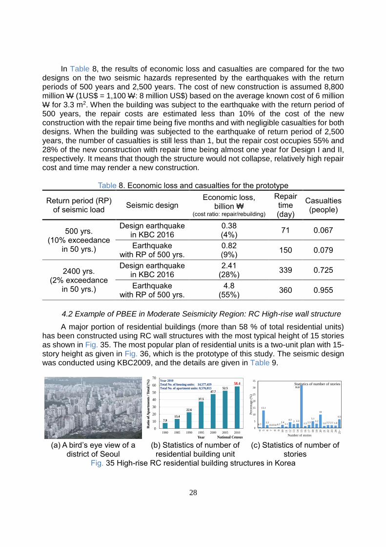
In Table 8, the results of economic loss and casualties are compared for the two designs on the two seismic hazards represented by the earthquakes with the return periods of 500 years and 2,500 years. The cost of new construction is assumed 8,800 million W (1US$ = 1,100 W: 8 million US$) based on the average known cost of 6 million W for 3.3 m2. When the building was subject to the earthquake with the return period of 500 years, the repair costs are estimated less than 10% of the cost of the new construction with the repair time being five months and with negligible casualties for both designs. When the building was subjected to the earthquake of return period of 2,500 years, the number of casualties is still less than 1, but the repair cost occupies 55% and 28% of the new construction with repair time being almost one year for Design I and II, respectively. It means that though the structure would not collapse, relatively high repair cost and time may render a new construction.

Table 8. Economic loss and casualties for the prototype

Return period (RP) of seismic load

Seismic design Economic loss,

billion ₩ (cost ratio: repair/rebuilding)

Repair time (day)

Casualties (people)

500 yrs. (10% exceedance

in 50 yrs.)

Design earthquake in KBC 2016

0.38 (4%)

71 0.067

Earthquake with RP of 500 yrs.

0.82 (9%)

150 0.079

2400 yrs. (2% exceedance

in 50 yrs.)

Design earthquake in KBC 2016

2.41 (28%)

339 0.725

Earthquake with RP of 500 yrs.

4.8 (55%)

360 0.955

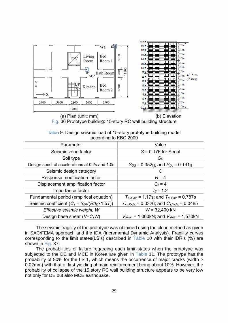
4.2 Example of PBEE in Moderate Seismicity Region: RC High-rise wall structure

A major portion of residential buildings (more than 58 % of total residential units) has been constructed using RC wall structures with the most typical height of 15 stories as shown in Fig. 35. The most popular plan of residential units is a two-unit plan with 15-story height as given in Fig. 36, which is the prototype of this study. The seismic design was conducted using KBC2009, and the details are given in Table 9.

(a) A bird’s eye view of a district of Seoul

(b) Statistics of number of residential building unit

(c) Statistics of number of stories

Fig. 35 High-rise RC residential building structures in Korea

7.9

13.4

22.6

37.5

47.752.5

58.4

0

10

20

30

40

50

60

70

1980 1985 1990 1995 2000 2005 2010

Rati

o o

f A

part

men

ts / T

ota

l (%

)

Year

Year 2010

Total No. of housing units: 14,577,419

Total No. of apartment units: 8,576,013

National Census

0.7

13.1

2.20.4 0.4 0.7

2.41.1

4.33 3.3

31.8

1.5 2.3

5.13.2

10

1.6 2.2 2.1 1.8

6.5

0

5

10

15

20

25

30

35

-4 5 6 7 8 9

10

11

12

13

14

15

16

17

18

19

20

21

22

23

24

25~

Per

centa

ge

(%)

Number of stories

Statistics of number of stories

29

(a) Plan (unit: mm) (b) Elevation Fig. 36 Prototype building: 15-story RC wall building structure

Table 9. Design seismic load of 15-story prototype building model according to KBC 2009

Parameter Value

Seismic zone factor S = 0.176 for Seoul

Soil type SC

Design spectral accelerations at 0.2s and 1.0s SDS = 0.352g; and SD1 = 0.191g

Seismic design category C

Response modification factor R = 4

Displacement amplification factor Cd = 4

Importance factor IE = 1.2

Fundamental period (empirical equation) Ta,X-dir. = 1.17s; and Ta,Y-dir. = 0.787s

Seismic coefficient (Cs = SD1/(R/IE×1.5T)) Cs,X-dir. = 0.0326; and Cs,Y-dir. = 0.0485

Effective seismic weight, W W = 32,400 kN

Design base shear (V=CsW) VX-dir. = 1,060kN; and VY-dir. = 1,570kN

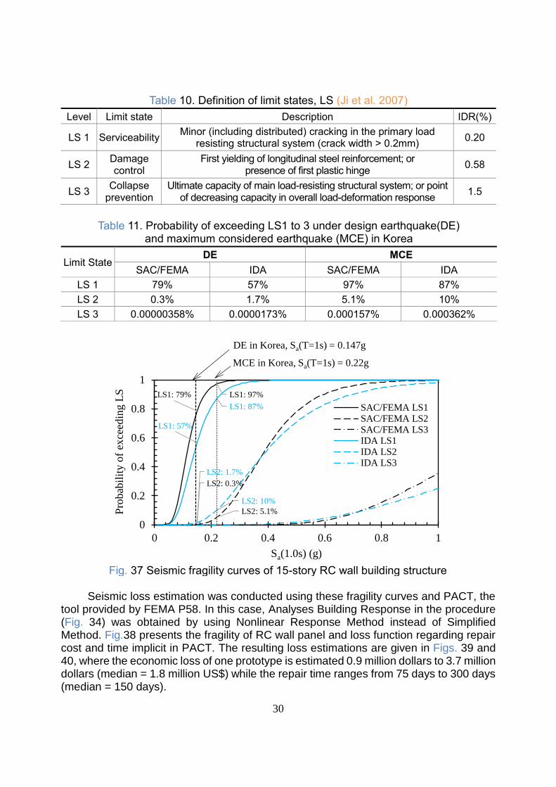
The seismic fragility of the prototype was obtained using the cloud method as given

in SAC/FEMA approach and the IDA (Incremental Dynamic Analysis). Fragility curves corresponding to the limit states(LS’s) described in Table 10 with their IDR’s (%) are shown in Fig. 37.

The probabilities of failure regarding each limit states when the prototype was subjected to the DE and MCE in Korea are given in Table 11. The prototype has the probability of 90% for the LS 1, which means the occurrence of major cracks (width > 0.02mm) with that of first yielding of main reinforcement being about 10%. However, the probability of collapse of the 15 story RC wall building structure appears to be very low not only for DE but also MCE earthquake.

30

Table 10. Definition of limit states, LS (Ji et al. 2007)

Level Limit state Description IDR(%)

LS 1 Serviceability Minor (including distributed) cracking in the primary load

resisting structural system (crack width > 0.2mm) 0.20

LS 2 Damage control

First yielding of longitudinal steel reinforcement; or presence of first plastic hinge

0.58

LS 3 Collapse

prevention Ultimate capacity of main load-resisting structural system; or point

of decreasing capacity in overall load-deformation response 1.5

Table 11. Probability of exceeding LS1 to 3 under design earthquake(DE) and maximum considered earthquake (MCE) in Korea

Limit State DE MCE

SAC/FEMA IDA SAC/FEMA IDA

LS 1 79% 57% 97% 87%

LS 2 0.3% 1.7% 5.1% 10%

LS 3 0.00000358% 0.0000173% 0.000157% 0.000362%

Fig. 37 Seismic fragility curves of 15-story RC wall building structure

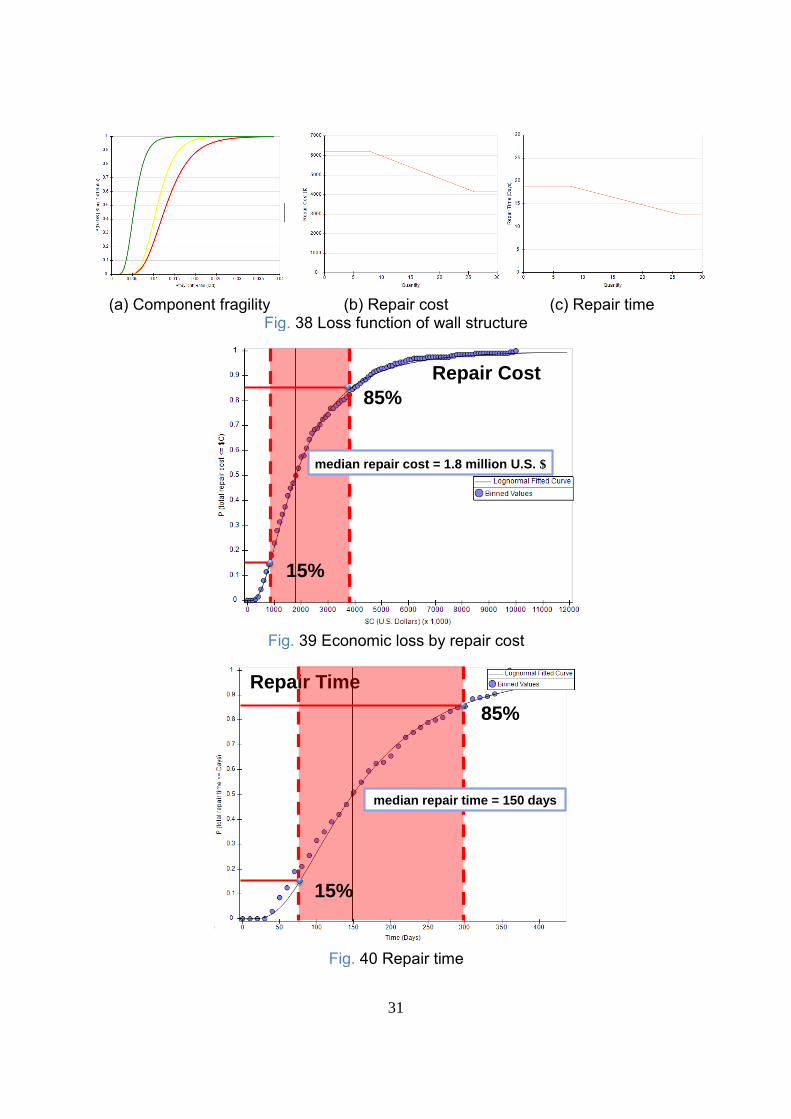
Seismic loss estimation was conducted using these fragility curves and PACT, the

tool provided by FEMA P58. In this case, Analyses Building Response in the procedure (Fig. 34) was obtained by using Nonlinear Response Method instead of Simplified Method. Fig.38 presents the fragility of RC wall panel and loss function regarding repair cost and time implicit in PACT. The resulting loss estimations are given in Figs. 39 and 40, where the economic loss of one prototype is estimated 0.9 million dollars to 3.7 million dollars (median = 1.8 million US$) while the repair time ranges from 75 days to 300 days (median = 150 days).

LS1: 79% LS1: 97%

LS2: 0.3%

LS2: 5.1%

LS1: 57%

LS1: 87%

LS2: 1.7%

LS2: 10%

0

0.2

0.4

0.6

0.8

1

0 0.2 0.4 0.6 0.8 1

Pro

bab

ilit

y o

f ex

ceed

ing L

S

Sa(1.0s) (g)

SAC/FEMA LS1SAC/FEMA LS2SAC/FEMA LS3IDA LS1IDA LS2IDA LS3

MCE in Korea, Sa(T=1s) = 0.22g

DE in Korea, Sa(T=1s) = 0.147g

31

(a) Component fragility (b) Repair cost (c) Repair time

Fig. 38 Loss function of wall structure

Fig. 39 Economic loss by repair cost

Fig. 40 Repair time

Repair Time

median repair time = 150 days

median repair cost = 1.8 million U.S. $

15%

85% 85%

15%

Repair Cost

Repair Time

median repair time = 150 days

median repair cost = 1.8 million U.S. $

15%

85% 85%

15%

Repair Cost

32

4.3 Expected range of force and deformation in a moderate seismicity region: South Korea

The experimental researches through the earthquake simulation tests to identify the seismic weakness of reinforced concrete (RC) nonseismic building structures designed only for gravity loads and to observe the seismic performance of RC residential building structures designed per the recent Korean seismic code are presented. Based on all these observations, expected ranges of force and deformation are summarized for code writers or engineers in moderate seismicity regions.

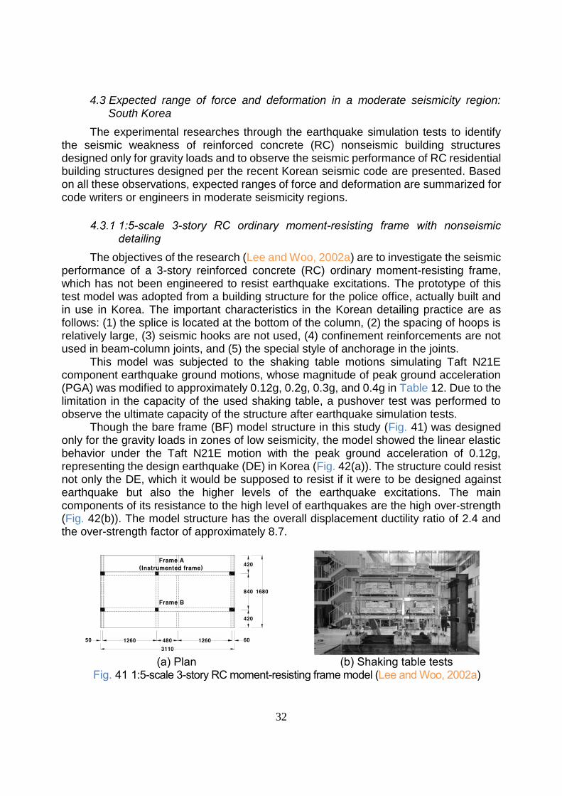
1:5-scale 3-story RC ordinary moment-resisting frame with nonseismic detailing

The objectives of the research (Lee and Woo, 2002a) are to investigate the seismic performance of a 3-story reinforced concrete (RC) ordinary moment-resisting frame, which has not been engineered to resist earthquake excitations. The prototype of this test model was adopted from a building structure for the police office, actually built and in use in Korea. The important characteristics in the Korean detailing practice are as follows: (1) the splice is located at the bottom of the column, (2) the spacing of hoops is relatively large, (3) seismic hooks are not used, (4) confinement reinforcements are not used in beam-column joints, and (5) the special style of anchorage in the joints.

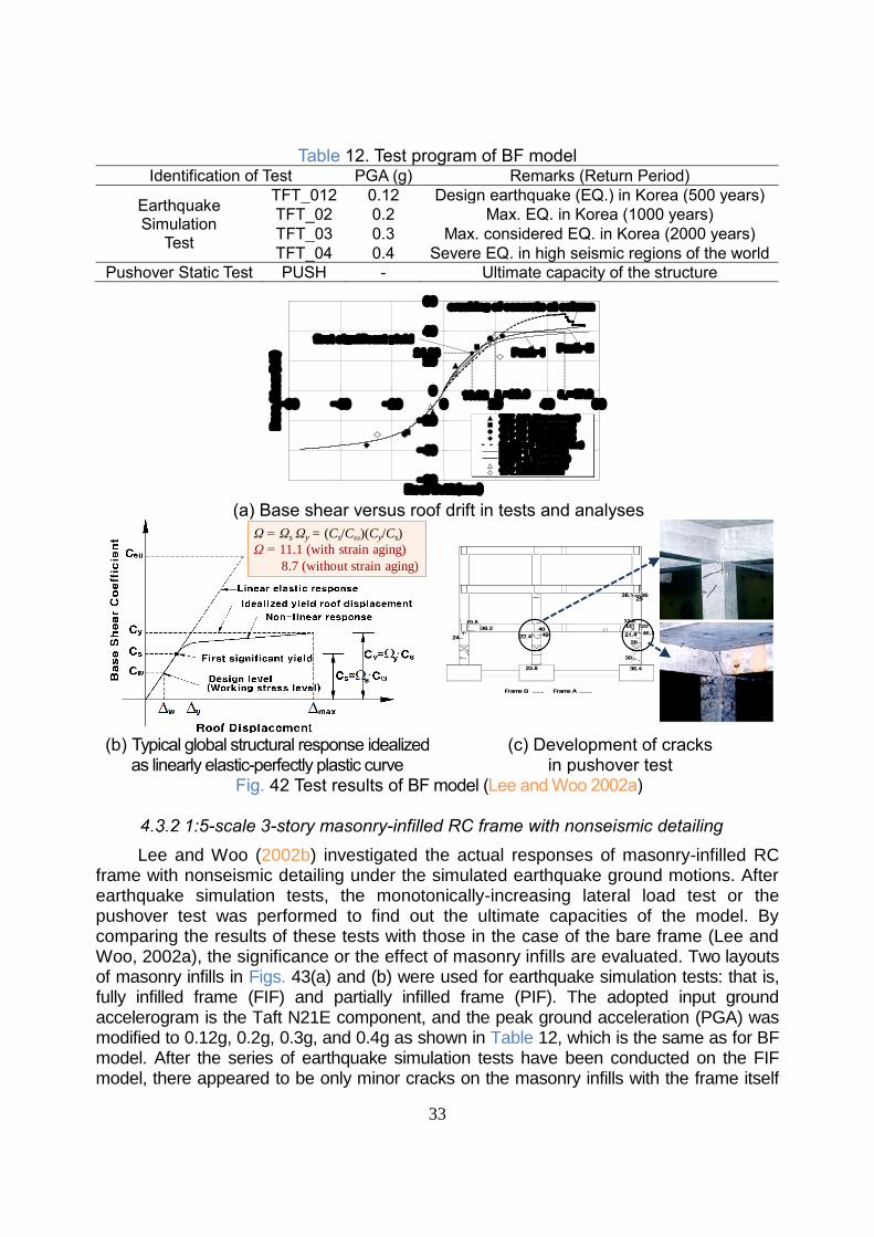
This model was subjected to the shaking table motions simulating Taft N21E component earthquake ground motions, whose magnitude of peak ground acceleration (PGA) was modified to approximately 0.12g, 0.2g, 0.3g, and 0.4g in Table 12. Due to the limitation in the capacity of the used shaking table, a pushover test was performed to observe the ultimate capacity of the structure after earthquake simulation tests.

Though the bare frame (BF) model structure in this study (Fig. 41) was designed only for the gravity loads in zones of low seismicity, the model showed the linear elastic behavior under the Taft N21E motion with the peak ground acceleration of 0.12g, representing the design earthquake (DE) in Korea (Fig. 42(a)). The structure could resist not only the DE, which it would be supposed to resist if it were to be designed against earthquake but also the higher levels of the earthquake excitations. The main components of its resistance to the high level of earthquakes are the high over-strength (Fig. 42(b)). The model structure has the overall displacement ductility ratio of 2.4 and the over-strength factor of approximately 8.7.

(a) Plan (b) Shaking table tests

Fig. 41 1:5-scale 3-story RC moment-resisting frame model (Lee and Woo, 2002a)

3110

12601260 480

840

420

420

1680

6050

Frame A

(Instrumented frame)

Frame B

33

Table 12. Test program of BF model Identification of Test PGA (g) Remarks (Return Period)

Earthquake Simulation

Test

TFT_012 0.12 Design earthquake (EQ.) in Korea (500 years)

TFT_02 0.2 Max. EQ. in Korea (1000 years)

TFT_03 0.3 Max. considered EQ. in Korea (2000 years)

TFT_04 0.4 Severe EQ. in high seismic regions of the world

Pushover Static Test PUSH - Ultimate capacity of the structure

(a) Base shear versus roof drift in tests and analyses

(b) Typical global structural response idealized as linearly elastic-perfectly plastic curve

(c) Development of cracks in pushover test

Fig. 42 Test results of BF model (Lee and Woo 2002a)

1:5-scale 3-story masonry-infilled RC frame with nonseismic detailing

Lee and Woo (2002b) investigated the actual responses of masonry-infilled RC frame with nonseismic detailing under the simulated earthquake ground motions. After earthquake simulation tests, the monotonically-increasing lateral load test or the pushover test was performed to find out the ultimate capacities of the model. By comparing the results of these tests with those in the case of the bare frame (Lee and Woo, 2002a), the significance or the effect of masonry infills are evaluated. Two layouts of masonry infills in Figs. 43(a) and (b) were used for earthquake simulation tests: that is, fully infilled frame (FIF) and partially infilled frame (PIF). The adopted input ground accelerogram is the Taft N21E component, and the peak ground acceleration (PGA) was modified to 0.12g, 0.2g, 0.3g, and 0.4g as shown in Table 12, which is the same as for BF model. After the series of earthquake simulation tests have been conducted on the FIF model, there appeared to be only minor cracks on the masonry infills with the frame itself

-60

-40

-20

0

20

40

60

-60 -40 -20 0 20 40 60

Roof Drift(mm)

Base S

hear(

kN

)

TFT_012 (Experiment)TFT_02 (Experiment)TFT_03 (Experiment)TFT_04 (Experiment)Pushover (Experiment)PUSH-I (Analysis)PUSH-II (Analysis)TFT_012(Analysis)TFT_04(Analysis)

y=20.0 u=47.2

crushing of concrete at column

first significant yield

10.82

24.33 Push-IPush-II

Ω = Ωs Ωy = (Cs/Cω)(Cy/Cs)

Ω = 11.1 (with strain aging)

8.7 (without strain aging)

34

remaining intact. Therefore, a portion of masonry infills was removed as shown in Fig. 43(b) and then this model, defined as PIF, was again subjected to the same series of earthquake simulation tests as the FIF.

The masonry infills can be beneficial to the seismic performance of the structure since the amount of the increase in strength appears to be greater than that in the induced earthquake inertia forces, while the deformation capacity of the global structure remains almost same regardless of the presence of the masonry infills. The maximum base shear of FIF, PIF, and BF under DE in Korea (TFT_012) was 32.0 kN, 37.3 kN, and 17.6 kN, respectively, in Fig. 44(a). These are 2.5 to 5.3 times the design base shear, 7.03 kN, according to the Korean seismic code. In Fig. 44(b), maximum interstory drift indices (IDI) in the FIF and PIF models under the varying peak input accelerations are shown and compared with those measured in the case of BF. The drifts of the PIF are greater than those of the FIF under the same level of input ground motions. However, IDI of neither FIF nor PIF exceeds the maximum value of 1.5% allowed in the Korean seismic code even under TFT_04.

Frame B

Frame A: Instrumented frame

Infill wall

Frame B

Frame A: Instrumented frame

Infill wall

(a) Shaking table test of FIF (b) Pushover test of PIF

Fig. 43 1:5-scale 3-story masonry-infilled RC frame model (Lee and Woo, 2002b)

(a) Base shear versus roof drift in tests (b) Change of maximum interstory drift

Fig. 44 1:5-scale 3-story masonry-infilled RC frame model (Lee and Woo, 2002b)

TFT_012 (design EQ.)

1.08

0.1880.1110.1060.042

0.51

0.30.28

0.24

1.68

0.77

0.26

0

0.4

0.8

1.2

1.6

2

TFT_012 TFT_02 TFT_03 TFT_04

Inte

rsto

ry d

rift

in

dex(%

)

FIF

PIF

BF

the maximum allowable under design earthquake: 1.5%

35

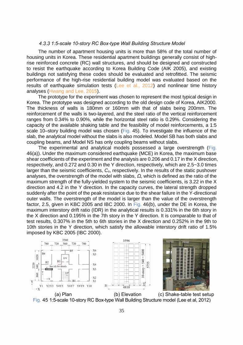
1:5-scale 10-story RC Box-type Wall Building Structure Model

The number of apartment housing units is more than 58% of the total number of housing units in Korea. These residential apartment buildings generally consist of high-rise reinforced concrete (RC) wall structures, and should be designed and constructed to resist the earthquake according to Korea Building Code (AIK 2005), and existing buildings not satisfying these codes should be evaluated and retrofitted. The seismic performance of the high-rise residential building model was evaluated based on the results of earthquake simulation tests (Lee et al., 2012) and nonlinear time history analyses (Hwang and Lee, 2015).

The prototype for the experiment was chosen to represent the most typical design in Korea. The prototype was designed according to the old design code of Korea, AIK2000. The thickness of walls is 180mm or 160mm with that of slabs being 200mm. The reinforcement of the walls is two-layered, and the steel ratio of the vertical reinforcement ranges from 0.34% to 0.90%, while the horizontal steel ratio is 0.29%. Considering the capacity of the available shaking table and the feasibility of model reinforcements, a 1:5 scale 10–story building model was chosen (Fig. 45). To investigate the influence of the slab, the analytical model without the slabs is also modeled. Model SB has both slabs and coupling beams, and Model NS has only coupling beams without slabs.

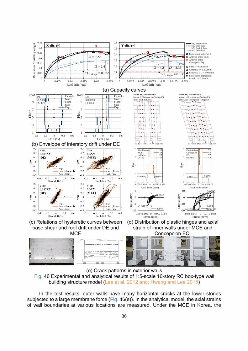
The experimental and analytical models possessed a large overstrength (Fig. 46(a)). Under the maximum considered earthquake (MCE) in Korea, the maximum base shear coefficients of the experiment and the analysis are 0.206 and 0.17 in the X direction, respectively, and 0.272 and 0.30 in the Y direction, respectively, which are 2.5~3.0 times larger than the seismic coefficients, Cs, respectively. In the results of the static pushover analyses, the overstrength of the model with slabs, Ω, which is defined as the ratio of the maximum strength of the fully-yielded system to the seismic coefficients, is 3.22 in the X direction and 4.2 in the Y direction. In the capacity curves, the lateral strength dropped suddenly after the point of the peak resistance due to the shear failure in the Y-directional outer walls. The overstrength of the model is larger than the value of the overstrength factor, 2.5, given in KBC 2005 and IBC 2000. In Fig. 46(b), under the DE in Korea, the maximum interstory drift ratio (IDR) in the analytical results is 0.331% in the 6th story in the X direction and 0.195% in the 7th story in the Y direction. It is comparable to that of test results, 0.307% in the 5th to 6th stories in the X direction and 0.252% in the 9th to 10th stories in the Y direction, which satisfy the allowable interstory drift ratio of 1.5% imposed by KBC 2005 (IBC 2000).

(a) Plan (b) Elevation (c) Shake-table test setup

Fig. 45 1:5-scale 10-story RC Box-type Wall Building Structure model (Lee et al, 2012)

36

(a) Capacity curves

(b) Envelope of interstory drift under DE

(c) Relations of hysteretic curves between

base shear and roof drift under DE and MCE

(d) Distribution of plastic hinges and axial strain of inner walls under MCE and

Concepcion EQ.

(e) Crack patterns in exterior walls

Fig. 46 Experimental and analytical results of 1:5-scale 10-story RC box-type wall building structure model (Lee et al. 2012 and; Hwang and Lee 2015)

In the test results, outer walls have many horizontal cracks at the lower stories

subjected to a large membrane force (Fig. 46(e)). In the analytical model, the axial strains of wall boundaries at various locations are measured. Under the MCE in Korea, the

0

0.05

0.1

0.15

0.2

0.25

0.3

0.35

0 0.005 0.01 0.015 0.02 0.025

Bas

e sh

ear

/ B

uil

din

g w

eig

ht

Roof drift (ratio)

SB, flexible-baseSB, fixed-baseNS, flexible-baseNS, fixed-base

X-dir. (+)

Cs, design = 0.072

Ω = 3.22

Ω = 2.4

0

0.1

0.2

0.3

0.4

0.5

0.6

0 0.0025 0.005 0.0075 0.01 0.0125 0.015

Bas

e sh

ear

/ B

uil

din

g w

eig

ht

Roof drift (ratio)

SB, flexible-baseSB, fixed-baseNS, flexible-baseNS, fixed-base

Y-dir. (+)

Cs, design = 0.108

Ω = 4.2 Ω = 3.36 Steel, ε = 0.002m/m

Shear stress degradation

in wall, ε = 0.01m/m

Concrete, ε = 0.002m/m

Concrete, εc,ult = 0.006m/m

Experiment under MCE

Analysis under MCE

Analysis under

Concepcion EQ.

1

3

5

7

9

11

-0.6 -0.3 0 0.3 0.6

Flo

or

Drift (%)

Flexible-

baseFixed-

baseExp.

RoofDE

in Korea

(X-dir.)

Roof

1

3

5

7

9

11

-0.6 -0.3 0 0.3 0.6

Flo

or

Drift (%)

Flexible-

baseFixed-

baseExp.

RoofDE

in Korea

(Y-dir.)

Roof Model SB, Flexible-base

Instant: 2.31s (max. roof drift (-X))

under MCE in Korea

Y1 Y2Y3 Y4Y5 Y6Y7 Y8Y9 Y10 Y1 Y2Y3 Y4Y5 Y6Y7 Y8Y9 Y10

Model SB, Flexible-base

Instant: 10.81s (max. roof drift (-X))

under 2010 Concepcion earthquake

-0.00119 0.00215

1

2

3

4

5

-0.003 -0.0015 0 0.0015 0.003

Flo

or

Axial Strain (m/m)

Y2

Y4

Y7

Y9

Flexible-base

MCE

in Korea

(2.31s)

-0.0154 0.0236

1

2

3

4

5

-0.03-0.02-0.01 0 0.01 0.02 0.03

Flo

or

Axial Strain (m/m)

Y2

Y4

Y7

Y9

Flexible-base

Concepcion

EQ.

(10.81s)

-0.0012

0.0015

-20

-10

0

10

-0.004-0.002 0 0.002 0.004

Str

ess

(M

Pa)

Strain (m/m)

X4Y4

0.0250

-0.0155-20

-10

0

10

-0.03-0.015 0 0.015 0.03

Str

ess

(MP

a)

Strain (m/m)

X4Y49s to 12s

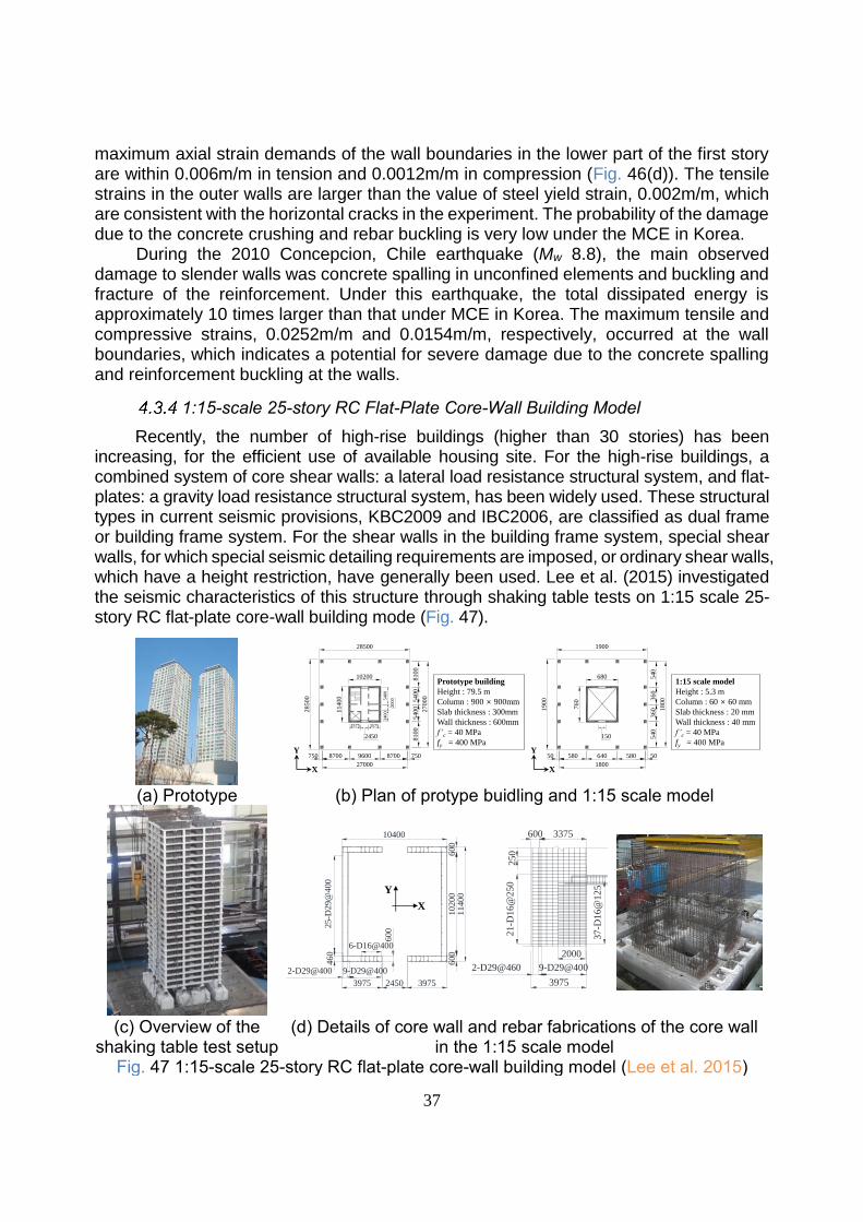
37

maximum axial strain demands of the wall boundaries in the lower part of the first story are within 0.006m/m in tension and 0.0012m/m in compression (Fig. 46(d)). The tensile strains in the outer walls are larger than the value of steel yield strain, 0.002m/m, which are consistent with the horizontal cracks in the experiment. The probability of the damage due to the concrete crushing and rebar buckling is very low under the MCE in Korea.

During the 2010 Concepcion, Chile earthquake (Mw 8.8), the main observed damage to slender walls was concrete spalling in unconfined elements and buckling and fracture of the reinforcement. Under this earthquake, the total dissipated energy is approximately 10 times larger than that under MCE in Korea. The maximum tensile and compressive strains, 0.0252m/m and 0.0154m/m, respectively, occurred at the wall boundaries, which indicates a potential for severe damage due to the concrete spalling and reinforcement buckling at the walls.

1:15-scale 25-story RC Flat-Plate Core-Wall Building Model

Recently, the number of high-rise buildings (higher than 30 stories) has been increasing, for the efficient use of available housing site. For the high-rise buildings, a combined system of core shear walls: a lateral load resistance structural system, and flat-plates: a gravity load resistance structural system, has been widely used. These structural types in current seismic provisions, KBC2009 and IBC2006, are classified as dual frame or building frame system. For the shear walls in the building frame system, special shear walls, for which special seismic detailing requirements are imposed, or ordinary shear walls, which have a height restriction, have generally been used. Lee et al. (2015) investigated the seismic characteristics of this structure through shaking table tests on 1:15 scale 25-story RC flat-plate core-wall building mode (Fig. 47).

(a) Prototype (b) Plan of protype buidling and 1:15 scale model

(c) Overview of the shaking table test setup

(d) Details of core wall and rebar fabrications of the core wall in the 1:15 scale model

Fig. 47 1:15-scale 25-story RC flat-plate core-wall building model (Lee et al. 2015)

28500

28500

8700 9600 8700 750

8100

5400

5400

8100

750

27000

27000

10200

11400

3400

20005

400

2450

35753575

Prototype building

Height : 79.5 m

Column : 900 × 900mm

Slab thickness : 300mm

Wall thickness : 600mm

f’c = 40 MPa

fy = 400 MPaY

X

1:15 scale model

Height : 5.3 m

Column : 60 × 60 mm

Slab thickness : 20 mm

Wall thickness : 40 mm

f’c = 40 MPa

fy = 400 MPaY

X

1900

1900

580 640 580 50

540

360

360

540

50

1800

1800

680

760

150

6-D16@400

60

0

9-D29@4002-D29@400

25

-D2

9@

40

04

60

60

01

02

00

60

01

14

00

3975 2450 3975

10400

Y

X

21

-D1

6@

25

0

37

-D1

6@

12

5

9-D29@4002-D29@460

3375

25

0

600

3975

2000

38

In Fig. 48(a), under the design earthquake in Korea (DE, 0.187XY), the base shear coefficients were 0.0361 in the X direction and 0.0518 in the Y direction, which are 1.5- and 2-fold larger than the design base shear coefficient of 0.0253, respectively. The strength increased gradually with the significant decrease of stiffness, and a large over-strength occurred (Fig. 48(b)). Under the DE (0.187XY), the maximum inter-story drift ratio was 0.31% from the 10th to 13th stories in the X direction and 0.30% from the 18th to 21th stories in the Y direction in Fig. 48(c), which satisfy the allowable inter-story drift ratio of 1.5% imposed by KBC 2009 (IBC 2006).

(a) Correlation between maximum roof drift and base shear coefficient

(b) Hysteretic relation of the base shear and roof displacement

(c) Envelope of interstory drift ratio (d) Distribution of story shear

(e) Strain distribution of the core wall

at the bottom of the first story under MCE (f) Relation of the moment and curvature (M-φ)

in core wall (X-dir.)

Fig. 48 Shake-table test results of a 1:15-scale 25-story RC flat-plate core-wall building model (Lee et al. 2015)

0

0.02

0.04

0.06

0.08

0.1

0 20 40 60

Bas

e sh

ear co

effi

cien

t, C

s

Roof displacement (mm)

XY ExcitationX Excitation

X-dir.

0.035g0.07g

0.154g 0.187g

0.3g0.4g

Ω = 1.43Cs, design = 0.0253

0

0.02

0.04

0.06

0.08

0.1

0 20 40 60

Bas

e sh

ear co

effi

cien

t, C

s

Roof displacement (mm)

XY ExcitationY Excitation

Y-dir.

0.035g

0.07g

0.154g0.187g 0.3g

0.4g

Ω = 2.05

Cs, design = 0.0253

-100

-50

0

50

100

-60 -30 0 30 60

Bas

e sh

ear

(kN

)

Roof displacement (mm)

Table

ExcitationNo

Excitation

0.07XY

Vmax = - 23.9kN

k = 4.71 kN/mm

X-dir.

-100

-50

0

50

100

-60 -30 0 30 60

Bas

e sh

ear

(kN

)

Roof displacement (mm)

Table

ExcitationNo

Excitation

0.187XY

Vmax = 41.9kN

k = 2.36 kN/mm

X-dir.

-100

-50

0

50

100

-60 -30 0 30 60

Bas

e sh

ear

(kN

)

Roof displacement (mm)

Table

ExcitationNo

Excitation

0.3XY

Vmax = - 67.9kN

k = 1.61 kN/mm

X-dir.

-100

-50

0

50

100

-60 -30 0 30 60

Bas

e sh

ear

(kN

)

Roof displacement (mm)

Table

ExcitationNo

Excitation

0.4XY

Vmax = - 70.5kN

k = 0.97 kN/mm

X-dir.

-100

-50

0

50

100

-60 -30 0 30 60

Bas

e sh

ear

(kN

)

Roof displacement (mm)

Table

Excitation

No

Excitation

0.07XY

Vmax = 26.5kN

k = 5.26 kN/mm

Y-dir.

-100

-50

0

50

100

-60 -30 0 30 60

Bas

e sh

ear

(kN

)

Roof displacement (mm)

Table

Excitation

No

Excitation

0.187XY

Vmax = 60.2kN

k = 3.67 kN/mm

Y-dir.

-100

-50

0

50

100

-60 -30 0 30 60

Bas

e sh

ear

(kN

)

Roof displacement (mm)

Table

Excitation

No

Excitation

0.3XY

Vmax = 79.9kN

k = 2.55 kN/mm

Y-dir.

-100

-50

0

50

100

-60 -30 0 30 60

Bas

e sh

ear

(kN

)

Roof displacement (mm)

Table

Excitation

No

Excitation

0.4XY

Vmax = 83.3kN

k = 1.79 kN/mm

Y-dir.

02468

1012141618202224262830

-0.02 -0.01 0 0.01 0.02

Sto

ry

Interstory drift ratio (rad)

0.187XY0.3XY0.4XY

Roof

22

18

14

10

6

X-dir.

No Excitation

1.5%

02468

1012141618202224262830

-0.02 -0.01 0 0.01 0.02

Sto

ry

Interstory drift ratio (rad)

0.187XY0.3XY0.4XY

Roof

22F

18F

14F

10F

6F

Y-dir.

No Excitation

1.5%38.5 -34.8

02468

1012141618202224262830

-90 -60 -30 0 30 60 90

Sto

ry

Shear force (kN)

0.187XY0.3XY0.4XY

Roof

22

18

14

10

6

Max. Roof Accel. Table Excitation

X-dir.

49.3 -77.5

02468

1012141618202224262830

-90 -60 -30 0 30 60 90

Flo

or

Shear force (kN)

0.187XY0.3XY0.4XY

Roof

22F

18F

14F

10F

6F

Max. Roof Accel. Table Excitation

Y-dir.

0.0014

-0.000180.0058

0.00078

0.00094

-0.00018

0.0078

0.0013

X-dir. (0.3XY)

인장변형(+)

압축변형(-)

Vx = 58.8 kN

Vy = 12.8 kN

Time = 14.04 secTension (+)

Compression (-)

X-dir.

Y-dir.φx-dir. = 0.0085rad/m

φx-dir.= 0.034rad/m(tension)

(compression)

-60

-30

0

30

60

-0.15 -0.075 0 0.075 0.15

Mo

men

t (k

Nm

)

Curvature (rad/m)

1.0 DLDL/3.59εy = 0.002εc = 0.003εc = 0.006

Short wall

φu = 0.041

φx-dir.=0.0085

φcl = 0.019

φx-dir. = 0.034

φy = 0.0104

εy

εc

εc

39

The model displayed behavior in the first mode during free vibration after the termination of excitation, and the maximum values of the base shear and roof drift in this duration can be either similar to or larger than the values of the maximum responses during the table excitation. The higher modes were observed in both the X and Y directions in the vertical distribution of story shear. When the roof acceleration reached a maximum, the effect of the second and third modes governed, and the largest story shear was apparent from the 14th to 21st stories instead of the first story (Fig. 48(d)).

In accordance with the displacement-based design method proposed in ACI 318-05, special boundary details were imposed on the short wall in the first story with the expected plastic rotation of θp = 0.00537 rad (Fig. 48(e)). No significant plastic deformation was observed under the MCE in Korea. At the bottom 70 mm of the first story, the measured maximum curvature when the end of the boundary element in the short wall is in compression is φx-dir. = 0.0085 rad/m, which is approximately 21% of 0.041 rad/m, the ultimate curvature corresponding to the expected compressive strain of 0.00638 m/m (Fig. 48(f)). This result, together with the findings mentioned above, implies that the design requirements on the boundary elements of the walls given in ACI 318-05 may be overly conservative, particularly for the wall design of high-rise RC building frames or dual-frame structures with more than 20 stories.

5. SUMMARY AND CONCLUSIONS

5.1 Summary

Characteristics of earthquake ground motions in moderate seismicity regions are as follows:

• The probability of collapse can be very low in moderate seismicity regions with that of non-structural damage being very high.

• The damages were concentrated to the region within the short epicentral distance.

• The duration is relatively short, so resonance effect can be minor. And, intensity of high-frequency contents is very high at near field but decays very rapidly as the epicentral distance increases.

• Spectral accelerations of high frequency are very high and can cause the brittle failure such as shear failure of short columns and crushing of window glasses.

• Spectral displacement can be significantly small when compared to the spectral acceleration. Therefore, flexible structures generally have a low probability of large inelastic excursions.

• The impact of high-frequency ground motions to the lower-frequency structures can cause non-vibratory unidirectional overload to the shear-critical members such as short columns.

• Typical building structures in a moderate seismicity region such as South Korea, which were not designed seismically, have retained a large overstrength, so it is not reasonable to assume all the non-seismically designed building structures would collapse as many media rouse the public to the unjustified fear.

40

The success of PBEE in high-seismicity regions as well as in moderate-seismicity regions depends on how we can estimate the actual behavior and loss reasonably. That is, every assumption in the analysis should be verified with experimental observation of structures. Estimation of earthquake load should be ascertained by the real records of EQ ground motions and the rationale for extrapolation of the ground motion prediction equation to the maximum magnitude earthquake should be provided. The followings are considered to be prerequisites for the success of PBEE in any cases.

• Estimation of actual seismic demands on the structural and nonstructural responses can be possible only by the provision of seismic hazard curves for all structures. Also, guides to input ground motions to be used for the linear and nonlinear analysis should be provided.

• Database of existing structures regarding design, construction, and maintenance should be established. Moreover, database of the mathematical behavior models, resistance capacity for all kinds of major structural and non-structural elements should be set up with their probability distributions.

• The linear and nonlinear behavior models of elements and joints should be verified through experiments, and the reliability in the prediction of overall structural behaviors using these models should be confirmed. Also, the user of the nonlinear software should have a full understanding of the nonlinear analysis and the limitations of the used software.

• Database should be set up for the derivation of fragility curves of structural and nonstructural elements and for estimation of economic losses due to the damages.

• To ensure the true realization of PBEE, the inspection process on the quality of design, construction, and maintenance should be established. For this, a reliable system of peer review should be provided.

5.2 Conclusions

• PBEE can be used as a tool to evaluate the appropriateness of the existing seismic code, which was developed mainly for the high-seismicity regions, and to adapt this code to the moderate-seismicity regions. To do this, first, the design of structures according to the requirements of the current codes, second, perform first- and second-generation PBEE on these designed structures. For example, each building structures (infilled masonry, or masonry structure, RC moment frame, steel moment frame, wall structure, dual structure, so on) designed exactly per the current prescriptive seismic codes are evaluated using PBEE procedure. Based on these results, appropriateness of performance factors such as R, Cd and Ω will be verified regarding the actual behaviors through PBEE procedure. Also, the maximum deformations in moderate-seismicity regions are estimated with the probability distribution and used to determine the appropriate requirements for seismic details, which will clearly lead to the alleviation of requirements for seismic details made mainly for the high-seismicity regions.

• September 12, 2016, Gyeongju earthquake has provided valuable data of earthquake ground motions representing the moderate-seismicity region. By analyzing and utilization of these data, it becomes possible to establish the

41

seismological model in Korean Peninsula. It is necessary to build up the seismic hazard map appropriate for Korean Peninsula by simulating the earthquake ground motion with this developed the seismological model and the probability theory. The research on the faults in Korean Peninsula should cover not only paleoseismic geological study on the faults developed over several million years, but also provide the information on the faults behaviors which occurred within Holocene period (11,000 years), including the return period of 2,500 years, 500 years, and much shorter durations because this information only can make a meaningful contribution to seismic design and retrofit.

• The earthquake tectonics in Korean Peninsula does not belong to the plate boundary or the plate boundary related intraplate, but belongs to the category of intraplate or mid-plate regions, whose slip rate is less than 0.1 mm/year. The earthquake in these regions are called small earthquakes whose maximum magnitudes will generally be 6.0~6.5, and do not show the surface ruptures with hidden faults. Because the historical catalog over the past 2,000 years in Korea cannot be used reliably to predict the maximum magnitude earthquakes in the return period of 2,500 years, it seems more reasonable to determine the design earthquake having the return period as short as possible, such as 500 years (10% probability of exceedance in 50 years).

• Because any building structure retains some minimum level of earthquake resistant capacity, it is a good approach to evaluate this level of resistance and to use this information for the seismic strengthening for the target maximum earthquake. Though there has been almost no severe earthquake disaster over the past several centuries in Korea, the news of devastated cities around the world due to the severe earthquakes might cause unjustified fears to Korean people and lead to over- or unnecessary design and construction, which should be avoided anyway.

• One example of the over- or unnecessary design and construction may be the use of dampers to retrofit low-rise school buildings in Korea. As shown on Sept. 12, 2016, Gyeongju earthquake, the characteristics of the near-source earthquake (maximum magnitude Mw ≤6.5) in moderate-seismicity regions can be described as an impulsive load. However, the efficacy of damper for this type of load is questionable and should be reevaluated and, if the response of the structure appears to be unsatisfactory, redesign and reconstruction should be conducted.

• Also, low-rise and high-frequency structures, subjected to a very high impulsive or implosive earthquake load due to the near-source earthquake, can lead to brittle shear failure of the critical beams and columns. Special design requirements to ensure the safety against this failure should be developed.

• Although the probability of collapse of building structures appears to be very low in moderate-seismicity regions, the failure of windows, dislocation of ceilings and falling of roof tiles were shown to be highly probable. Since a major portion of the economic loss is due to these non-structural failures, it is necessary to develop appropriate design requirements specific to the moderate-seismicity regions.

42

ACKNOWLEDGMENTS The research presented herein was supported by the National Research Foundation of Korea (NRF-2009-0078771), the Ministry of Land, Infrastructure and Transport of Korea (17AUDP-B066083-05), the Ministry of Public Safety and Security of Korea (MPSS-NH-2013-70), and the Korea University Grant. The authors are grateful for these supports. REFERENCES References are listed alphabetically for each part as follows: Building codes and guidelines:

ACI Committee 318 (2005) Building code requirements for structural concrete and commentary (ACI 318-05), American Concrete Institute, Detroit.

AIK (2000), AIK 2000, Architectural Institute of Korea (AIK), Seoul, Korea. (in Korean) AIK (2005), Korean Building Code. KBC 2005, Seoul, Korea. (In Korean) AIK (2009), Korean Building Code. KBC 2009, Seoul, Korea. (In Korean) AIK (2016), Korean Building Code. KBC 2016, Seoul, Korea. (In Korean) ASCE (2010), Minimum design loads for buildings and other structures, ASCE/SEI 7-10,

American Society of Civil Engineers (ASCE), Reston, Virginia, US. ASCE (2013), Seismic evaluation and retrofit of existing buildings, ASCE 41-13,

American Society of Civil Engineers (ASCE), Reston, Virginia, US. ATC (1996a), Improved Seismic Design Criteria for California Bridges: Provisional

Recommendations: ATC-32. National Bureau of Standards: Washington DC, 1996. ATC (1996b), Seismic evaluation and retrofit of existing concrete buildings: ATC-40,

Applied Technology Council (ATC), Redwood City, CA. FEMA (1996), NEHRP guidelines for the seismic rehabilitation of buildings, FEMA 273

Commentary, Federal Emergency Management Agency (FEMA), Washington DC. FEMA (2000), Prestandard and commentary for the seismic rehabilitation of buildings.

Report No. FEMA-356, Washington, DC, 2000. FEMA (2012), Seismic performance assessment of buildings. Report FEMA P-58,

Federal Emergency Management Agency, Washington DC, U.S.A. ICC (2000) International Building Code, IBC 2000, International Code Council, Country Club Hills, IL. ICC (2006) International Building Code, IBC 2006, International Code Council, Country Club Hills, IL. SEAOC (1995), Vision 2000, Performance based seismic engineering of buildings, Vols.

I and II: Conceptual framework, Structural Engineers Association of California (SEAOC), Sacramento, CA.

Chapter 1:

Par. 2, Page 1 ~ Par. 2, Page 2 excerpted from: Günay, S., & Mosalam, K. M. (2013) PEER performance-based earthquake engineering

methodology, revisited. Journal of Earthquake Engineering, 17(6), 829-858.

43

Chapter 2:

Par. 4, Page 2 excerpted from: Krawinkler, H., & Miranda, E. (2004). Performance-based Earthquake Engineering.

Chapter 9 of Earthquake Engineering: from Engineering Seismology to Performance-based Engineering. Bozorgnia and VV Bertero, Editors, CRC Pres.

Par. 5, Page 2 ~ Par. 2, Page 3 excerpted from: Porter, K. A. (2003). “An overview of PEER’s performance-based earthquake

engineering methodology,” Proceedings of ninth international conference on applications of statistics and probability in civil engineering.

Par. 1, Page 4 ~ Par. 6, Page 6 excerpted from:

Moehle, J., & Deierlein, G. G. (2004). “A framework methodology for performance-based earthquake engineering”, The 13th world conference on earthquake engineering, Paper No. 679, pp. 3812-3814, August 1-6, Vancouver, B.C., Canada.

Chapter 3:

Pars. 1~3, Page 7 / Pars. 1~3, Page 8 excerpted from: Scholz, C. H. (2002). The mechanics of earthquakes and faulting. Cambridge university press.

Pars. 1~5, Page 9 excerpted from: Nordenson, G. J., & Bell, G. R. (2000), “Seismic design requirements for regions of

moderate seismicity”, Earthquake spectra, 16(1), 205-225.

Pars. 1~3, Page 10 excerpted from: Frankel, A. (1995). “Mapping seismic hazard in the central and eastern United

States”. Seismological Research Letters, 66(4), 8-21.

Pars. 1~2, Page 14 excerpted from: Houng, S.E., & Hong, T.K. (2013). “Probabilistic analysis of the Korean historical earthquake

records,” Bulletin of the Seismological Society of America, 103(5), 2782-2796.

Pars. 1~3, Page 16 excerpted from: Hong, T.K., Lee, J.H., Kim, W.H., Hahm, I.K., Woo, N.C., & Park, S.J. (2017). “The 12

September 2016 ML 5.8 midcrustal earthquake in the Korean Peninsula and its seismic implications,” Geophysical Research Letters. 44(7), 3131-3138.

Others: Bakun, W. H., and M. G. Hopper (2004). “Magnitudes and locations of the 1811-1812

New Madrid, Missouri and the 1886 Charleston, South Carolina, earthquakes,” Bull. Seismol. Soc. Am. 94, 64–75.

Boore, D. M., Atkinson, G. M. (2008) “Ground-Motion Prediction Equations for the Average Horizontal Component of PGA, PGV, and 5%-Damped PSA at Spectral Periods between 0.01 s and 10.0 s,” Earthquake Spectra. 24(1), pp 99-138.

Boore, D. M., Campbell, K. W., & Atkinson, G. M. (2010). “Determination of stress parameters for eight well-recorded earthquakes in eastern North America,” Bulletin of the Seismological Society of America. 100(4), 1632-1645.

Cornell, C. A. (1968) “Engineering seismic risk analysis,” Bulletin of the Seismological Society of America. 58(5), pp. 1583-1606.

Fardis, M.N. (2014) Comments on the seismic design provisions of the Korean Building Code 2009. (Opinion paper)

44

Johnston, A. C. (1996). “Seismic moment assessment of earthquakes in stable continental regions—III. New Madrid 1811-1812, Charleston 1886 and Lisbon 1755,” Geophys. J. Int., 126, 314–344.

Korean Broadcasting System (KBS), available from: http://news.kbs.co.kr/news/view.do?ncd=3366101, last accessed 29 June 2017. (in Korean)

Korea Meteorological Administration (KMA), available from: http://www.kma.go.kr/, last accessed October 2016. (in Korean)

Kramer, S. L. (1996). Geotechnical Earthquake Engineering, Prentice Hall. New York. Lam, N. (2014) Displacement based assessment of structures for low and moderate

seismic regions (Opinion paper). Lee, C.H. (2017) “Earthquake Engineering Analysis of Ground Accelerations Measured

in the 912 Gyeong-ju Earthquake,” Journal of the Koran society of Civil Engineers, 65(4), 8-13. (in Korean)

McGuire, R. K. (1976) “Probabilistic seismic hazard analysis and design earthquakes: closing the loop,” Bulletin of the Seismological Society of America, 85(5), pp. 1275-1284.

NEMA (2012), Active fault map and seismic hazard map. National Emergency Management Agency, Report No. NEMA-NH-2009-24. (in Korean)

Ohmynews, available from: http://www.ohmynews.com/NWS_Web/View/at_pg.aspx?CNTN_CD=A0002243576, last accessed 29 June 2017. (in Korean)

USGS, available from: https://earthquake.usgs.gov/earthquakes/eventpage/us20005iis#finite-fault, last accessed 29 June 2016. (in Korean)

Yonhapnews, available from: http://www.yonhapnews.co.kr/bulletin/2016/09/19/0200000000AKR20160919070351053.html, last accessed 29 June 2017. (in Korean)

YTN, available from: http://www.ytn.co.kr/_ln/0115_201609131800184070, last accessed 29 June 2017. (in Korean)

Chapter 4:

Chung, K.R., Chung, H.J., Kang, M.S., Kim, S.H., and Park, K.M. (2013) "Eliminating special seismic boundary of special shear wall system using NLTHA." Korea Concrete Institute Conference, 2013 Fall. Sokcho, Korea: Korea Concrete Institute. (in Korean)

Ji, J., Elnashai, A.S., & Kuchma, D.A. (2009). Seismic fragility relationships of reinforced concrete high‐rise buildings. The Structural Design of Tall and Special Buildings, 18(3), 259-277.

Hwang, K. R., & Lee, H. S. (2015). Seismic performance of a 10-story RC box-type wall building structure. Earthquake and Structures, 9(6), 1193-1219.

Lee, H. S., and Woo, S. W. (2002a) “Seismic performance of a 3-story RC frame in a low-seismicity region”, Engineering Structures, 24(6), 719-734.

Lee, H. S., and Woo, S. W. (2002b). “Effect of masonry infills on seismic performance of a 3‐storey R/C frame with non‐seismic detailing”, Earthquake Engineering & Structural Dynamics, 31(2), 353-378.

Lee, H. S., Hwang, S. J., Lee, K. B., Kang, C. B., Lee, S. H., and Oh, S. H. (2012). “Earthquake Simulation Tests on a 1: 5 Scale 10-Story RC Residential Building Model,” The 15th World Conference on Earthquake Engineering (15WCEE), Lisbon, Portugal.

Lee, H. S., Hwang, K. R., & Kim, Y. H. (2015). “Seismic performance of a 1: 15‐scale 25‐story RC flat‐plate core‐wall building model,” Earthquake Engineering & Structural Dynamics, 44(6), 929-953.