pdf (434 kb) - iopscience - institute of physics

Journal of Physics Conference Series

OPEN ACCESS

Determination of Distance from a 2D PictureTo cite this article J Gravesen et al 2006 J Phys Conf Ser 52 005

View the article online for updates and enhancements

You may also likeDark matter spin-dependent limits forWIMP interactions on 19F by PICASSOBerta Beltran and the Picassocollaboration

-

(g-2) factors for muon and electron andthe consequences for QEDF H Combley

-

New insights into particle detection withsuperheated liquidsS Archambault F Aubin M Auger et al

-

This content was downloaded from IP address 1267714251 on 23122021 at 2059

Determination of Distance from a 2D Picture

J Gravesen15 B Lassen2 R Melnik26 B Picasso3 R Piche4

N Radulovic2 and L X Wang2

1 Department of Mathematics Technical University of DenmarkMatematiktorvet Building 303S DK-2800 Kgs Lyngby Denmark2 Mads Clausen Institute University of Southern Denmark Grundvigs Alle 150DK-6400 Soslashnderborg Denmark3 Scuola Normale Superiore Pisa Italy4 Department of Mathematics Tampere University of Technology FIN-33101 TampereFinland

E-mail JGravesenmatdtudk bennymcisdudk rmelnikwluca

radullemcisdudk wanglinxiangmcisdudk bpicassosnsit

robertpichetutfi

Abstract An optical device is used to scan a cavity In a single incident the scanner produceswhat can be considered a blurred image of the intersection curve between a plane and the cavityMathematically the image represents an intensity function and that is obtained by integratinga certain kernel along the intersection curve

We suggest methods to determine the kernel and subsequently the intersection curve giventhe image The methodology is tested with some success using an artificial but realistic kerneland some synthetic images produced by this kernel

Keywords Optical distance measurement inverse problemMSC 65K10 68T45 78A55

1 The problem

At the 47th Study Group with Industry in Grasten Denmark Martin Valvik from UnisensorInc presented a problem concerning an optical scanner (Figure 1)

The scanner is meant to be moved inside a cavity and find its shape The idea is first todetermine a sequence of cross sections and then assemble these cross sections to give the fullinner surface of the cavity The plane which defines the cross section is fixed relative to thescanner so the position of the scanner needs to be known in order to place the cross sectioncorrectly in space This is not the problem that concerns us here though We only want to findthe cross section relative to the scanner

The scanner is (approximately) axisymmetric and light is transmitted in a ring round theaxis down to a cone from where it is reflected radially out in a plane (approximately) If weimagine that the scanner is inserted into some cavity then the light from the scanner will hit (apart of) the sides of the cavity and form a ldquocurve of lightrdquo the above mentioned cross sectionThe light will be reflected back from the sides of the cavity to the cone where it will be reflectedupwards through a lens and finally make an image in the image plane

5 Corresponding author6 Present address Wilfrid Laurier University 75 University Avenue West Waterloo Ontario N2L 3C5 Canada

Institute of Physics Publishing Journal of Physics Conference Series 52 (2006) 46ndash57doi1010881742-6596521005 Mathematics for Industry in Denmark

46copy 2006 IOP Publishing Ltd

Image plane

r

Light plane

Side of cavity

Light ray

Lens

yx

z

θr

Figure 1 The scanner inside a cavity the light path and cylinder coordinates

The problem is to determine the cross section from the image So we know the intensityfunction I(x y) where (x y) are coordinates in the image plane and we want to determine thefunction r(θ z) where r is the distance from the axis of the scanner θ is an angle around thecenter-axis (the z-axis) ie (r θ z) are cylinder coordinates

We assume that the light is transmitted in a plane so the z dependence disappears and weare left with the task of determining the univariate function r(θ) from the intensity functionI(x y) = I(ρ cos θ ρ sin θ) where (ρ θ) are polar coordinates in the image plane

The paper is organized as follows In Section 2 we explain the methodology presently used bythe company and the assumptions the method is based upon and using the same assumptions wesuggest an improvement to the method in Section 3 we make a model based on more generalassumptions Mathematically we assume that the image is created by integration a certainkernel along the intersection curve In Section 4 we explain how the kernel can be determinedexperimentally We note that the problem at hand is related to shape-from-shading problemsand we explore this connection further in Section 5 In this section we also explain how by usingthe kernel mentioned above we can obtain the intersection curve from an image by solving anoptimization problem In Section 6 we give an example of this procedure and the results arepresented in Section 8 We did not have enough data to determine the kernel so instead wepostulated a kernel we deemed reasonable In Section 7 we use the singular value decompositionto check how well the postulated kernel could explain the image created by a point sourceFinally in Section 9 we have the conclusions

The people working on the problem was Ole Brink-Kjaeligr Kasper Doring Jens Graven JensKarlsson Poul G Hjorth Benny Lassen Roderick Melnik Henrik Gordon Petersen BrunoPicasso Robert Piche Janis Rimshans Nenad Radulovic Peter Roslashgen Martin Valvik LinxiangWang Stefan Wolff

We will like take this opportunity to thank Unisensor and in particular Martin Valvik forcontributing the problem answering many questions during the study group and even organizingnew measurements when requested

2 The present method and an improvement

The methodology presently used by the company builds upon a number of assumptions

(i) It is assumed that the light from the scanner is reflected in a plane orthogonal to the axisso the only part of the cavity that can be ldquoseenrdquo is the intersection of the cavity with thisplane ie we only need to determine a function of one variable r(θ)

(ii) More severely it is assumed that the image intensity along a radial ray ie I(x y) =I(ρ cos θ ρ sin θ) depends only on the distance r = r(θ) in this direction

47

The point of view is that the point ρmax where the function I(ρ) = I(ρ cos θ ρ sin θ) has itsmaximum is the image of the point r(θ) and that there is a one-to-one correspondence betweenr and ρmax The function ρmax rarr r can subsequently be determined experimentally Thescanner will never be exactly axisymmetric but that only means that ρmax also depends on θie we need to experimentally determine the function (θ ρmax) rarr r

Given the assumptions 1) and 2) above the basic problem is to determine the maximumintensity I(ρ) = I(ρ cos θ ρ sin θ) along a radial ray First of all it is necessary to smooth thefunction before the maximum is determined cf Figure 4 where the lefthand graph shows theintensity along a radial ray Furthermore the intensity function is often flat and hence it can bedifficult and error prone to determine the maximum

Instead of considering the maximum as the image of the point r(θ) it is better to considerthe whole function I(ρ) = I(ρ cos θ ρ sin θ) as the result of a measurement and then use a morerobust and easily calculated number to characterize the function An obvious choice is to usethe first moment (center of mass)

ρ0 =

intinfin

0 ρI(ρ) dρintinfin

0 I(ρ) dρ (1)

as ρ0 is insensitive to noise there is no need to perform any smoothing The two functionsr(ρ0) and r(ρmax) are both decreasing and exhibit the same qualitative behaviour It is ofcourse possible to incorporate asymmetry in this setting too and determine the function r(θ ρ0)experimentally

3 The basic model

We consider a cavity given by the equation r = r(θ z) and assume that the light from thescanner is reflected diffusively with intensity α(r z) from the point with cylinder coordinates(r(θ z) θ z) If (x y) rarr G0(x y r θ z) is the intensity function created by a (unit) light sourcesituated at the point (r θ z) then the intensity in the image plane created by the intensityfunction α(r z) is found by integrating G(x y r θ z) = α(r z)G0(x y r θ z) over the surfaceof the cavity

I(x y) =

int 2π

0

intinfin

minusinfin

G(x y r(θ z) θ z) dz dθ (2)

A small remark is appropriate here The intensity α at a point on the surface depends not onlyon the distance but also on the angle between the light ray and the normal of the surface Alsothe integration should be with respect to surface area and not dz dθ What happens is thatlight transmitted in small angle ∆θ∆z can be distributed on a larger area of the surface andthus the intensity falls but when we then integrate with respect to surface area we regain allthe intensity so the two corrections cancels each other and (2) is correct

In practice there would only be a small z-interval where G(x y r(θ z) θ z) = 0 If we canassume that the light from the scanner only emits light in a plane orthogonal to the symmetryaxis then we can drop the z dependence and we have diffuse light emitted from a curve withequation r = r(θ) and we have a kernel G(x y r θ) = α(r)G0(x y r θ) where α(r) = 1r Theintensity is now

I(x y) =

int 2π

0G(x y r(θ) θ) dθ (3)

and we want to determine the function r(θ) There are now two tasks

(i) Determine the kernel G(x y r θ)

(ii) Provide a procedure that determines the function r(θ) from the intensity I(x y)

48

Figure 2 Inverted images the reference the thin stick and the difference

4 The kernel

If we assume that the scanner is symmetric then we have

G(x y r θ) = G(x cos θ minus y sin θ x sin θ + y cos θ r 0) (4)

so we need only to determine G(x y r 0)It is tempting to try to calculate the kernel from first principles It is indeed possible to use

geometric optics and follow a ray from a point in the ldquolightrdquo-plane through the scanner until ithits the image plane This gives a map from a sphere centered at the light source to the imageplane and the area deformation gives (a part of) the intensity ie the kernel The actuallycomputations are rather involved and it will be hard (but not impossible) to get a usable result

Unfortunately there is a more severe and fundamental problem When the ray hits a boundarybetween two media eg at the cone or at the outside of scanner a fraction of the light istransmitted and the other fraction gets reflected These fractions depends not only on the anglebetween the ray and the surface normal but also on the polarization of the light cf [7] Thatin turn depends on the light source the material of the cavity and optical details of the scannerand would in practice be impossible to determine

Instead we suggest to determine the kernel experimentally The method would be to use thescanner not to make a ldquopicturerdquo of a cavity but to make a series of pictures of a thin stick inknown distances rk from the axis of the scanner If the stick is sufficiently thin then we cansubtract a reference picture (a picture of nothing) and get a direct measurement of the kernelG(xi yj rk 0) where (xi yj) are the coordinates of the pixels of the CCD-camera see Figure 2Sufficiently thin would mean thinner than the final resolution that the scanner is supposed toprovide

After obtaining the values G(xi yj rk 0) the next step is to approximate the kernel functionwith a suitable smooth function for example a trivariate tensor product B-spline

For a fixed r we can see from Figure 2 that the support of the kernel is concentrated in arelatively small area Hence we concentrate the knots in that same area cf Figure 3 Whenwe now let r vary two things happens The shape of the intensity function changes and theposition of the support is shifted along the x-axis We have two suggestions to model the kernelThe first is as a straight forward B-spline cf [3]

G(x y r 0) asymp f(x y r) =sumijk

f ijkNn1

i (xx)Nn2

j (yy)Nn3

k (r r) (5)

where Nni (t t) denotes the ith basis function of degree n on the knot vector t and the knots x

in the x-direction is chosen such that they can accommodate all positions of the support The

49

coefficients f ijk are chosen such that they minimize the 2-normsumijk

(f(xi yj rk) minus G(xi yj rk 0))2 (6)

This is a linear problem which is easily solved For the second suggestion we shift the origin tothe first moment (the center of mass) of the intensity function and propose an approximationto the kernel of the following form

G(x y r 0) asymp f(x minus x0(r) y r) (7)

where x0 and f are B-splines

x0(r) =sum

i

xi0N

n0

i (r r0) (8)

f(x y r) =sumijk

f ijkNn1

i (xx)Nn2

j (yy)Nn3

k (r r) (9)

The coefficients xi0 and f ijk are chosen such that they minimize the 2-norm

sumk

(x0(rk) minus

sumij xiG(xi yj rk 0)sumij G(xi yj rk 0)

)2

(10)

and sumijk

(f(xi minus x0(rk) yj rk) minus G(xi yj rk 0))2 (11)

This leads to two linear problems which are easily solved It will in both cases be necessary toexperiment with the degrees (n0) n1 n2 n3 and the number and placements of the knots (r0)xy r The first suggestion needs more coefficients but the structure is simpler so subsequentcalculations are easier

There is potentially another advantage of the form (5) Suppose the r-dependents of thekernel is so simple that it can be approximated by a low degree polynomial of degree K Thenit is possible to pre-compute some values we will later need in a minimization procedure wherewe try to find the function r(θ) that makes

intG(xi yj r(θ) θ) dθ fits the measurement best

Indeed if r(θ) is a uniform B-spline r(θ) =sum

alNm (θ minus 2πn) then

G(xi yj r(θ) θ) = f(xi cos θ minus yj sin θ xi sin θ + yj cos θ r(θ))

=sumijk

f ijkNn1

i (xi cos θ minus yj sin θ)Nn2

j (xi sin θ + yj cos θ)

(sum

aNm

(θ minus

2π

n

))k

For θ isin [2πn 2π( + 1)n] only m + 1 of the basis functions Nm

(θ minus 2π

n

)are non-zero so we

have int 2π

0G(xi yj r(θ) θ) dθ =

Ksumk=1

sum1k

G12k

ij a1a2 ak (12)

where the inner sum is over sequences 1 le 2 le le k with lk minus l1 le m and where the

coefficients G11k

ij can be precomputed If the degrees m and K are sufficiently small then

the number of coefficients G11k

ij is manageable

50

0

50

100

Figure 3 To the left the rotated image with the knots lines to the right the quadratic B-splineapproximating the intensity

As a small test we have rotated the image in Figure 2 with 600 times 600 pixels and valuesbetween 0 and 117 We have used a quadratic tensor product B-spline to approximate theintensity function and the knot-vectors were

x = 0 400 450 470 490 510 530 550 570 600

y = 0 200 250 280 290 300 310 320 350 400 600

The result can be seen in Figure 3 The approximation error measured in the max-norm the2-norm and the 1-norm became

I minus finfin = 156 I minus f2 = 127 I minus f1 = 050

5 The procedure

We now have our approximation of the kernel G(x y r θ) ie we assume that

G(x y r θ) = f(x cos θ minus y sin θ x sin θ + y cos θ r) or (13)

G(x y r θ) = f((x minus x0(r)) cos θ minus y sin θ (x minus x0(r)) sin θ + y cos θ r) (14)

Given measured intensities I(xi yj) we want to determine a function r(θ) such that (3) issatisfied This is a non-trivial problem which is closely related to the so-called shape-from-shading problems In what follows we highlight briefly this connection Recall that our originalproblem described in Section 1 requires determining the shape of an object (a cavity in our case)from its two-dimensional images In its essence this is a special case of the classical shape-from-shading problem that has been discussed extensively in the literature [4 10 12 9 6 13] Basicsteps upon which the model construction for this problem and the procedure for its solution canbe based are as follows As before we will denote by I(x y) the intensity function of the imageIn order to determine the shape (a surface) of the object on the basis of the given image(s)one could relate the intensity (or the brightness) function of the image (given for exampleat each pixel (xi yj)) and the reflectance map that keeps the information on the real three-dimensional object The form of the reflectance map under which the images are generatedfrom the (unknown) 3D depth map has to be assumed as the only measurements producedby the scanner that can be analysed are the images themselves [13] A natural way to relatesuch images to the 3D object is via the surface depth (the distance or the hight) function in

51

the z-direction denoted further by u(x y) Then images of the same object given in the (xy)-plane will differ from each other by shape gradients ζ1 = partupartx and ζ2 = partuparty which areessential characteristics of the 3D object Hence one can view the information based on the setof functions u(x y) ζ1 and ζ2 as the information from which among other things the shapeof cavity can be extracted As the cavity shape is modelled in (2) by using function r(θ z)that enters the kernel of the integral equation the development of specific algorithms to obtainr from (u ζ1 ζ2) would be dependent on the specific form of kernel approximation in model(2) In order to determine u (and hence ζ1 and ζ2) recall that ldquoshadingrdquo a 2D characteristic ofthe object is represented mathematically by the image intensity I(x y) while ldquoshaperdquo a 3Dcharacteristic of the object is represented by the surface reflectance denoted here by H(ζ1 ζ2)The latter specifies the reflectance of a surface under consideration as a function of its orientationand both functions are related to each other by the image irradiance equation (eg [4])

I(x y) = H(ζ1(x y) ζ2(x y)) ζ1 = partupartx ζ2 = partuparty (15)

Problem (15) can be reformulated as the first order partial differential equation underappropriate assumptions on function H According to the Unisensor representative theassumption of perfectly matt (Lambertian) surface is reasonable hence we can use Lambertrsquos lawto determine a possible approximation to H In particular if a part of the surface with normalvector n = (minusuxminusuy 1) is illuminated in the direction l = (l1 l2 l3) the emitted radiance (thatwill determine the image produced by the scanner) is given by the cosine of the angle betweenn and l namely by (l3 minus l1ux minus l2uy)(u

2x + u2

y + 1)12 Therefore if for example l = (0 0 1)then under the assumption of unit albedo and unit power of the source light we arrive at theHamilton-Jacobi equation of the form (eg [9])

(u2x + u2

y + 1)minus12 = I(x y) (16)

In a more general situation l = (sin σl cos τl sin σl sin τl cos σl) where σl and τl are slant andtilt angles [2] The latter expression can be simplified if we consider cross-sectional areas onlyas depicted in Fig 2 to l = (cos τl sin τl 0) Then accounting for the surface albedo (denotedby λ) and the incident light flux (denoted by ρ) we obtained the following approximation tofunction H(ζ1 ζ2)

H(ζ1 ζ2) = λρminusζ1 cos τl minus ζ2 sin τlradic

1 + ζ21 + ζ2

2

(17)

Given (15) and (17) we obtain the first order PDE with respect to the distance (or surface depth)function u(x y) According to the Unisensor representative all parameters in this equation aremeasurable including grayness of the surface λ the incident light flux ρ (a characteristic of thescanner) while σl and τl can be estimated on the basis of the image intensity map (given by thecompany) physical characteristics of the surface and the scanner (eg [12 13] and referencestherein) A natural way to solve the resulting problem is by applying the variational approach(eg [4 8]) In this case the cost functional can be defined as follows

W =

int intΩ

[I minus H]2 + micro1

[(part2u

partx2

)2

+ 2

(part2u

partxparty

)2

+

(part2u

party2

)2]

+ micro2Φ

dxdy rarr min (18)

where the second term (known as the ldquodeparture-from-smoothnessrdquo error) is a regularizing termas the problem at hand is an ill-posed problem (see [4 12 5]) The first term (known as theldquoring of lightrdquo or ldquobrightnessrdquo error) comes into consideration directly from equation (15) whilethe third term is added to ensure integrability of the constrained optimization problem

Models (2) and (17) are related in a sense that both are attempts to construct a model thatrelates the information about a 3D object and the information about 2D images of that object

52

While in the former case we use a geometric analysis of the problem to construct the modelthe latter approach is ultimately based on a more conventional idea of using energy functionals(eg [1]) In our case instead of using a more conventional approximation (17) we attempt toapproximate the kernel of the reflectance map as it is stated by our formula (2) In this casewe model r(θ) (rather than function u(x y)) as a uniform periodic B-spline

r(θ) =

nsumk=1

akNm

( n

2πθ minus k

) (19)

where N is the B-spline of degree m on the uniform knot sequence minus1 0 1 and n issufficiently large to give the resolution we want The coefficients ak are chosen such that the2-norm sum

ij

(I(xi yj) minus

int 2π

0G(xi yj r(θ) θ) dθ

)2

is minimized As the integral in (18) is replaced by a finite sum the third term (18) is not neededFurthermore since the problem will be solved in terms of coefficients ak which will determiner(θ) by (19) we use the quadratic term ak

2 to regularize the problem In its essence ourapproach has some similarities with the Greenrsquos function approach to shape-from-shading (eg[11]) Now the task at hand is the following optimisation problem

minimizesumij

(I(xi yj) minus

int 2π


)2

+ microak2 (20)

where micro is a parameter and middot is a suitable seminorm common choices include

ak2 =

sumk

a2k ak

2 =sum

k

(ak minus akminus1)2 ak

2 =sum

k

(ak minus 2akminus1 + akminus2)2

An important aspect of this type of problems is to obtain a good initial guess for r(θ) Thescanner will be moved slowly inside the cavity so we would have a series of images ie intensityfunctions from which we want to determine planar sections of the cavity ie r(θ) We expectthe planar section of two subsequent measurements to be very similar so the result of theoptimization of one measurement would be a very good initial guess for the next To bootstrapthis procedure and have a good guess for the very first image one could use prior knowledge ofthe cavity or the simplified procedure suggested in section 2

In Section 6 we give an example of this procedure We did not have sufficient data to makea reasonable B-spline model of the kernel so instead we postulate a kernel with an exponentialdecay and a 1r dependence

We conclude this section with the following remark The problem at hand is a strongly non-linear problem and it would be advantageous to reduce it (at least for some special cases) to asequence of linear problems For model (17) it can be done if we use the assumption that thereal shape of the object is smooth Then the equation I(x y) = H(ζ1 ζ2) can be approximatedby using Taylorrsquos expansion of the reflectance function (eg [10]) As a result it is easy to findthe Fourier transforms Fζ1 and Fζ2 in terms of the Fourier transform of of u(x y) This allowsto relate the Fourier spectrum of the image and the Fourier transform of the surface FindingFourierrsquos inverse of Fu will allow to estimate the object shape This simplification should beuseful when the Unisensor needs to analyse sufficiently smooth surfaces without substantialirregularities

53

0 20 40 60 80 100 1200

01

02

03

04

05

06

07

08

0 50 100 150 200 250 300 350 4000

02

04

06

08

1

12

14

Figure 4 To the left the radial part f(ρ) and to the right the angular part g(α) of intensitydistribution I(ρ α)

6 Case study example

For the case study we make some changes to the situation in Section 5 Instead of Cartesiancoordinates (x y) in the image plane we use polar coordinates (ρ α) and instead of using B-splines to describe the kernel we just postulate a kernel of the form

G(ρ α r θ) = Aeminusk1(ρminusk3r)2minusk2(αminusθ)2 = Aeminusk1(ρminusk3r)2eminusk2(αminusθ)2 (21)

ie the product of two Gaussian The parameters A k1 and k2 are chosen such that theGaussian approximates the the functions f(ρ) and g(α) from Figure 4 The result was A = 345k1 = 0002 and k2 = 001 We had only data for three unknown values of r so we had no waysof estimating k3 and we just put k3 = 1 This gives us a predicted intensity as follows

H =

int 2π

0345eminus0002(ρminus1r(θ))2minus001(αminusθ)2 dθ (22)

The function r is represented by a vector r = (r1 r2 rn) (can be thought as a discretisationin θ) and as regularization term we chose r2 = 2π

n

sumni=1(ri)

2 So the functional to minimisehas the following form int

infin

ρ=0

int 2π

α=0

[I minus H]2 + micror2

dαdρ rarr min (23)

where I(α ρ) is the measured image intensityAt this stage we took r = 1 corresponding to a unit circular object and created a synthetic

image using (22) We then tested the optimization procedure by letting the initial guess of r berandomly chosen around r = 1 with a relative error of 5 The maximal initial relative errorwe have tried is 20 Numerical experiments show that the optimization gives a quite goodestimation of the actual value of r as shown in figure 6 to 8

7 Considerations regarding the Singular Values Decomposition

In this section we provide details of our SVD-based procedure to verify how well the kernelpostulated in Section 6 can explain the image created by a point source We have discretized ρand α

ρ = ρi i = 1 N

α = αj j = 1 M

54

Figure 5 The assumption that I(ρ α) factors as is given by (24)

The intensity distribution I(x y) obtained processing the CCD picture generated by a sourcein position (r θ) has been transformed into a discrete polarndashcoordinate function I(ρi αj) we

denote by I isin RNtimesM the matrix Iij equiv I(ρi αj)

The assumption (see Fig5) that I(ρ α) factors as

I(ρ α) = f(ρ) middot g(α) (24)

corresponds to the fact that the matrix I has rank 1 Of course the numerical matrix I has fullrank anyway we can get a measure of ldquohow farrdquo is that matrix from having rank 1 by analysingthe singular values decomposition (SVD) of I In fact

I = USV t with U isin RNtimesN S isin R

NtimesM V isin RMtimesM

where U and V are unitary matrices and S = diag(σi) i = 1 minNM The numbers

σ1 ge σ2 ge middot middot middot ge 0 are the singular values of I Denote by ui and vi the ith column of the matricesU and V respectively If σ2 σ1 then I is well approximated by the matrix I1 = σ1 middotu1v

t1 which

has rank 1 it holds that I minus I12 le σ2 In this case σ1 middot u1 and v1 can be taken as a discreteversion of f(ρ) and g(α) respectively

Indeed our calculations showed that there were at least 10 singular values not negligible inthat case the matrix is well approximated by I10 =

sum10i=k σkukv

tk that has rank 10 and is such

that I minus I102 le σ11 If it is possible to find ten pairs of simple functions (fk gk) such thatσkuk asymp fk(ρi) and vk asymp gk(αi) then

sumk fk(ρ)gk(α) is a good approximation to the kernel This

has not been investigated in further detail Note also that for this procedure to be useful inpractice the r-dependence of the kernel should be simple

8 Results of computations

To find optimal values for micro and n in (23) we chose to fix micro and then carry out calculations forn = 20 40 and 80 We did calculations for micro = 10minus6 10minus3 005 and 01 In order to estimatethe error in the minimized function we used the L2 norm on the difference between the exactfunction (Z = 1) and the minimized function Those numbers are shown in Table 1 togetherwith the time it took to carry out the minimizations The best value we found was micro = 005 andthe more discretisation points the better In Figure 6 to 8 the initial guess and the minimizedfunction are shown for different values of micro

The target function is extremely simple (a constant) as is the kernel so it is not possibleto draw any hard conclusions regarding the usuability of the procedure That will require morerealistic data and extensive testing

55

0 100 200 300096

097

098

099

1

101

102

103

104

Angle (degree)

Dis

tanc

e

MinimizedInitial guess

210

240

270

300


Figure 6 To the left a plot of the initial guess and the minimized distance function as afunction of angle to the right a section of a plot the initial guess and minimized function formicro = 10minus6 and n = 80

0 100 200 300097

098

099

1

101

102

103

104

Angle (Degree)

Dis

tanc

e


10

240

270

300

3


Figure 7 To the left a plot of the initial guess and the minimized distance function as afunction of angle to the right a section of a plot the initial guess and minimized function formicro = 005 and n = 80

Figure 8 A plot of the the initial guess and minimized function for micro = 005 and n = 80 Theinitial guess was generated with 20 random noise

9 Discussion and conclusion

We have demonstrated that the image produced by the scanner can be calculated by integratinga kernel along the ldquocurve of lightrdquo cf (3) The kernel can for a fixed r be represented well bya tensor product B-spline of a reasonable size cf (5) or (7)

56

micro n 20 40 8010minus1 022 17 sec 016 61 sec 011 464 sec005 017 12 sec 012 52 sec 008 90 sec10minus3 029 6 sec 015 36 sec 009 179 sec10minus6 03 5 sec 027 6 sec 017 80 sec

Table 1 The relative error and timing for different values of n and micro

As an other approach the singular value decomposition suggest that it is possible to describethe kernel as the sum of the products of ten pairs of univariate functions cf Section 7 So itmight be possible to use something more simple than the tensor product B-spline descriptionsthe univariate functions above would have to be described by a few parameters But we havenot investigated that

We did not have enough data to model the r dependence of the kernel so there is a need formore work here first of all images of ldquopoint sourcesrdquo in known distances are needed

Using a variational approach we have shown that it is possible to recapture the ldquocurve of lightrdquofrom the image As the r dependence was unknown we used an artificial but realistic kerneland we expect to get similar results using a more correct kernel Once more it is necessary todo extensive testing with real data

The timings given in Section 8 are not encouraging but improvements can be made Thefunction r(θ) depends linearly on the coefficients ak so it is not hard to get the gradient andHessian of the objective function given in (20) all it takes is to differentiate (13) or (14) withrespect to r ie we only have to differentiate a number of B-splines Access to the gradient andHessian will speed the optimization up substantially as will an implementation in C or FortranAlso it is perhaps possible to pre-compute a substantial part of the objective function cf (12)Finally since we deal with an inverse problem some prior knowledge of the cavity should helpimprove the performance of the methodologies developed and tested in this contribution

References[1] Chan TF Variational PDE models in image processing Notices of the AMS 50(1) 2003 14ndash26[2] Chojnacki W Brooks MJ Gibbins D Revisiting Pentlandrsquos estimator of light source direction J Opt

Soc Am A 11 1994 118ndash124[3] de Boor C A Practical Guide to Splines Springer-Verlag New York 2001[4] Horn BKP and Brooks MJ Shape from Shading MIT Press Cambridge MA 1989[5] Hsieh J-W et al Wavelet-based shape from shading Graphical Models and Image Processing 57(4) 1995

343ndash362[6] Jones AG and Taylor CJ Robust shape from shading Image and Vision Computing 12(7) 1994

411ndash421[7] Landau LD and Lifshitz EM Electrodynamics of Continuous Media Course of Theoretical Physics

Vol 8 Pergamon Press Oxford 1960[8] Lepsky O Hu C and Shu C-W Analysis of the discontinuous Galerkin method for Hamilton-Jacobi

equations Appl Numerical Mathematics 33 2000 423ndash434[9] Lions PL Rouy E and Tourin A Shape-from-Shading viscosity solutions and edges Numerische

Mathematik 64(3) 1993 323ndash353[10] Pentland AP Linear shape from shading Int J of Computer Vision 4 1990 153ndash162[11] Torreao J R A A Greenrsquos function approach to shape from shading Pattern Recognition 34 2001

2367ndash2382[12] Zheng Q and Chellappa R Estimation of illuminant direction albedo and shape from shading IEEE

Trans on Pattern Analysis and Machine Intelligence 13(7) 1991 680ndash702[13] Zhao W and Chellappa R Symmetric shape-from-shading using self-ratio image Int J of Computer

Vision 45(1) 2001 55ndash75

57

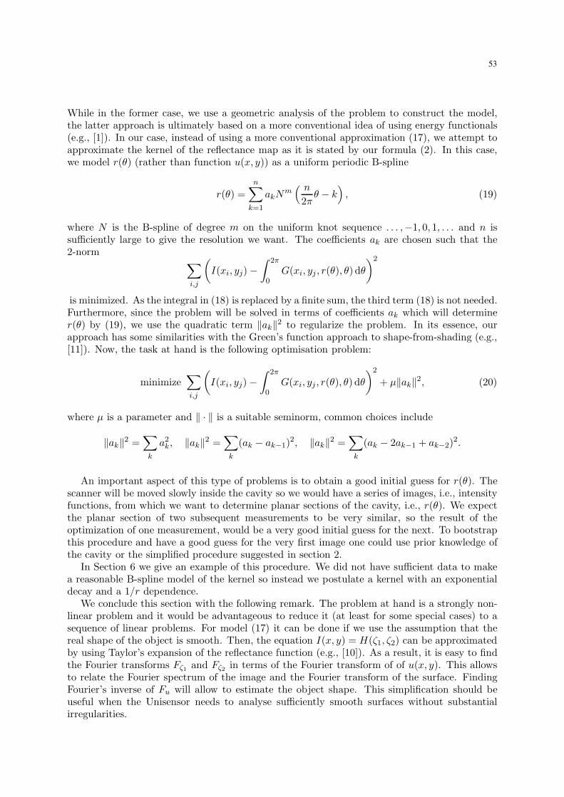
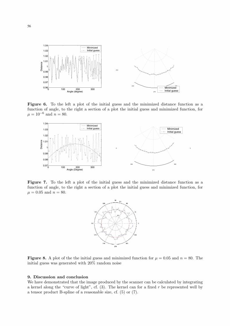
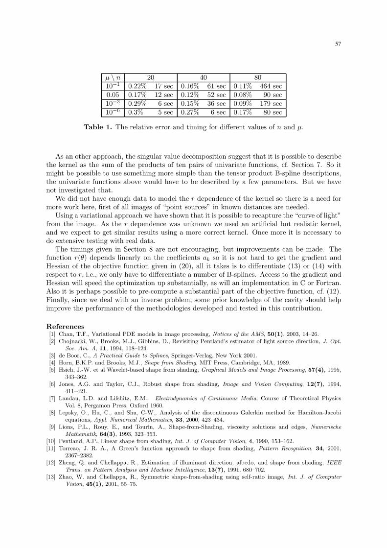Determination of Distance from a 2D Picture

J Gravesen15 B Lassen2 R Melnik26 B Picasso3 R Piche4

N Radulovic2 and L X Wang2

1 Department of Mathematics Technical University of DenmarkMatematiktorvet Building 303S DK-2800 Kgs Lyngby Denmark2 Mads Clausen Institute University of Southern Denmark Grundvigs Alle 150DK-6400 Soslashnderborg Denmark3 Scuola Normale Superiore Pisa Italy4 Department of Mathematics Tampere University of Technology FIN-33101 TampereFinland

E-mail JGravesenmatdtudk bennymcisdudk rmelnikwluca

radullemcisdudk wanglinxiangmcisdudk bpicassosnsit

robertpichetutfi

Abstract An optical device is used to scan a cavity In a single incident the scanner produceswhat can be considered a blurred image of the intersection curve between a plane and the cavityMathematically the image represents an intensity function and that is obtained by integratinga certain kernel along the intersection curve

We suggest methods to determine the kernel and subsequently the intersection curve giventhe image The methodology is tested with some success using an artificial but realistic kerneland some synthetic images produced by this kernel

Keywords Optical distance measurement inverse problemMSC 65K10 68T45 78A55

1 The problem

At the 47th Study Group with Industry in Grasten Denmark Martin Valvik from UnisensorInc presented a problem concerning an optical scanner (Figure 1)

The scanner is meant to be moved inside a cavity and find its shape The idea is first todetermine a sequence of cross sections and then assemble these cross sections to give the fullinner surface of the cavity The plane which defines the cross section is fixed relative to thescanner so the position of the scanner needs to be known in order to place the cross sectioncorrectly in space This is not the problem that concerns us here though We only want to findthe cross section relative to the scanner

The scanner is (approximately) axisymmetric and light is transmitted in a ring round theaxis down to a cone from where it is reflected radially out in a plane (approximately) If weimagine that the scanner is inserted into some cavity then the light from the scanner will hit (apart of) the sides of the cavity and form a ldquocurve of lightrdquo the above mentioned cross sectionThe light will be reflected back from the sides of the cavity to the cone where it will be reflectedupwards through a lens and finally make an image in the image plane

5 Corresponding author6 Present address Wilfrid Laurier University 75 University Avenue West Waterloo Ontario N2L 3C5 Canada

Institute of Physics Publishing Journal of Physics Conference Series 52 (2006) 46ndash57doi1010881742-6596521005 Mathematics for Industry in Denmark

46copy 2006 IOP Publishing Ltd

Image plane

r

Light plane

Side of cavity

Light ray

Lens

yx

z

θr











47




ρ0 =

intinfin


0 I(ρ) dρ (1)


3 The basic model


I(x y) =

int 2π

0

intinfin

minusinfin




I(x y) =

int 2π

0G(x y r(θ) θ) dθ (3)




48


4 The kernel










f ijkNn1

i (xx)Nn2

j (yy)Nn3

k (r r) (5)



49






x0(r) =sum

i

xi0N

n0

i (r r0) (8)

f(x y r) =sumijk

f ijkNn1

i (xx)Nn2

j (yy)Nn3

k (r r) (9)


sumk

(x0(rk) minus


)2

(10)

and sumijk








=sumijk

f ijkNn1



(sum

aNm

(θ minus

2π

n

))k


(θ minus 2π

n

)are non-zero so we

have int 2π


Ksumk=1

sum1k

G12k

ij a1a2 ak (12)


coefficients G11k



ij is manageable

50

0

50

100



x = 0 400 450 470 490 510 530 550 570 600

y = 0 200 250 280 290 300 310 320 350 400 600



5 The procedure





51




2x + u2


(u2x + u2

y + 1)minus12 = I(x y) (16)



1 + ζ21 + ζ2

2

(17)


W =

int intΩ


[(part2u

partx2

)2

+ 2

(part2u

partxparty

)2

+

(part2u

party2

)2]

+ micro2Φ

dxdy rarr min (18)



52


r(θ) =

nsumk=1

akNm

( n

2πθ minus k

) (19)


ij

(I(xi yj) minus

int 2π


)2



minimizesumij

(I(xi yj) minus

int 2π


)2

+ microak2 (20)


ak2 =

sumk

a2k ak

2 =sum

k


2 =sum

k





53

0 20 40 60 80 100 1200

01

02

03

04

05

06

07

08

0 50 100 150 200 250 300 350 4000

02

04

06

08

1

12

14






H =

int 2π



n

sumni=1(ri)


infin

ρ=0

int 2π

α=0







ρ = ρi i = 1 N

α = αj j = 1 M

54











t1 which



sum10i=k σkukv








55

0 100 200 300096

097

098

099

1

101

102

103

104

Angle (degree)

Dis

tanc

e


210

240

270

300



0 100 200 300097

098

099

1

101

102

103

104

Angle (Degree)

Dis

tanc

e


10

240

270

300

3






56

















57

Image plane

r

Light plane

Side of cavity

Light ray

Lens

yx

z

θr











47




ρ0 =

intinfin


0 I(ρ) dρ (1)


3 The basic model


I(x y) =

int 2π

0

intinfin

minusinfin




I(x y) =

int 2π

0G(x y r(θ) θ) dθ (3)




48


4 The kernel










f ijkNn1

i (xx)Nn2

j (yy)Nn3

k (r r) (5)



49






x0(r) =sum

i

xi0N

n0

i (r r0) (8)

f(x y r) =sumijk

f ijkNn1

i (xx)Nn2

j (yy)Nn3

k (r r) (9)


sumk

(x0(rk) minus


)2

(10)

and sumijk








=sumijk

f ijkNn1



(sum

aNm

(θ minus

2π

n

))k


(θ minus 2π

n

)are non-zero so we

have int 2π


Ksumk=1

sum1k

G12k

ij a1a2 ak (12)


coefficients G11k



ij is manageable

50

0

50

100



x = 0 400 450 470 490 510 530 550 570 600

y = 0 200 250 280 290 300 310 320 350 400 600



5 The procedure





51




2x + u2


(u2x + u2

y + 1)minus12 = I(x y) (16)



1 + ζ21 + ζ2

2

(17)


W =

int intΩ


[(part2u

partx2

)2

+ 2

(part2u

partxparty

)2

+

(part2u

party2

)2]

+ micro2Φ

dxdy rarr min (18)



52


r(θ) =

nsumk=1

akNm

( n

2πθ minus k

) (19)


ij

(I(xi yj) minus

int 2π


)2



minimizesumij

(I(xi yj) minus

int 2π


)2

+ microak2 (20)


ak2 =

sumk

a2k ak

2 =sum

k


2 =sum

k





53

0 20 40 60 80 100 1200

01

02

03

04

05

06

07

08

0 50 100 150 200 250 300 350 4000

02

04

06

08

1

12

14






H =

int 2π



n

sumni=1(ri)


infin

ρ=0

int 2π

α=0







ρ = ρi i = 1 N

α = αj j = 1 M

54











t1 which



sum10i=k σkukv








55

0 100 200 300096

097

098

099

1

101

102

103

104

Angle (degree)

Dis

tanc

e


210

240

270

300



0 100 200 300097

098

099

1

101

102

103

104

Angle (Degree)

Dis

tanc

e


10

240

270

300

3






56

















57




ρ0 =

intinfin


0 I(ρ) dρ (1)


3 The basic model


I(x y) =

int 2π

0

intinfin

minusinfin




I(x y) =

int 2π

0G(x y r(θ) θ) dθ (3)




48


4 The kernel










f ijkNn1

i (xx)Nn2

j (yy)Nn3

k (r r) (5)



49






x0(r) =sum

i

xi0N

n0

i (r r0) (8)

f(x y r) =sumijk

f ijkNn1

i (xx)Nn2

j (yy)Nn3

k (r r) (9)


sumk

(x0(rk) minus


)2

(10)

and sumijk








=sumijk

f ijkNn1



(sum

aNm

(θ minus

2π

n

))k


(θ minus 2π

n

)are non-zero so we

have int 2π


Ksumk=1

sum1k

G12k

ij a1a2 ak (12)


coefficients G11k



ij is manageable

50

0

50

100



x = 0 400 450 470 490 510 530 550 570 600

y = 0 200 250 280 290 300 310 320 350 400 600



5 The procedure





51




2x + u2


(u2x + u2

y + 1)minus12 = I(x y) (16)



1 + ζ21 + ζ2

2

(17)


W =

int intΩ


[(part2u

partx2

)2

+ 2

(part2u

partxparty

)2

+

(part2u

party2

)2]

+ micro2Φ

dxdy rarr min (18)



52


r(θ) =

nsumk=1

akNm

( n

2πθ minus k

) (19)


ij

(I(xi yj) minus

int 2π


)2



minimizesumij

(I(xi yj) minus

int 2π


)2

+ microak2 (20)


ak2 =

sumk

a2k ak

2 =sum

k


2 =sum

k





53

0 20 40 60 80 100 1200

01

02

03

04

05

06

07

08

0 50 100 150 200 250 300 350 4000

02

04

06

08

1

12

14






H =

int 2π



n

sumni=1(ri)


infin

ρ=0

int 2π

α=0







ρ = ρi i = 1 N

α = αj j = 1 M

54











t1 which



sum10i=k σkukv








55

0 100 200 300096

097

098

099

1

101

102

103

104

Angle (degree)

Dis

tanc

e


210

240

270

300



0 100 200 300097

098

099

1

101

102

103

104

Angle (Degree)

Dis

tanc

e


10

240

270

300

3






56

















57


4 The kernel










f ijkNn1

i (xx)Nn2

j (yy)Nn3

k (r r) (5)



49






x0(r) =sum

i

xi0N

n0

i (r r0) (8)

f(x y r) =sumijk

f ijkNn1

i (xx)Nn2

j (yy)Nn3

k (r r) (9)


sumk

(x0(rk) minus


)2

(10)

and sumijk








=sumijk

f ijkNn1



(sum

aNm

(θ minus

2π

n

))k


(θ minus 2π

n

)are non-zero so we

have int 2π


Ksumk=1

sum1k

G12k

ij a1a2 ak (12)


coefficients G11k



ij is manageable

50

0

50

100



x = 0 400 450 470 490 510 530 550 570 600

y = 0 200 250 280 290 300 310 320 350 400 600



5 The procedure





51




2x + u2


(u2x + u2

y + 1)minus12 = I(x y) (16)



1 + ζ21 + ζ2

2

(17)


W =

int intΩ


[(part2u

partx2

)2

+ 2

(part2u

partxparty

)2

+

(part2u

party2

)2]

+ micro2Φ

dxdy rarr min (18)



52


r(θ) =

nsumk=1

akNm

( n

2πθ minus k

) (19)


ij

(I(xi yj) minus

int 2π


)2



minimizesumij

(I(xi yj) minus

int 2π


)2

+ microak2 (20)


ak2 =

sumk

a2k ak

2 =sum

k


2 =sum

k





53

0 20 40 60 80 100 1200

01

02

03

04

05

06

07

08

0 50 100 150 200 250 300 350 4000

02

04

06

08

1

12

14






H =

int 2π



n

sumni=1(ri)


infin

ρ=0

int 2π

α=0







ρ = ρi i = 1 N

α = αj j = 1 M

54











t1 which



sum10i=k σkukv








55

0 100 200 300096

097

098

099

1

101

102

103

104

Angle (degree)

Dis

tanc

e


210

240

270

300



0 100 200 300097

098

099

1

101

102

103

104

Angle (Degree)

Dis

tanc

e


10

240

270

300

3






56

















57






x0(r) =sum

i

xi0N

n0

i (r r0) (8)

f(x y r) =sumijk

f ijkNn1

i (xx)Nn2

j (yy)Nn3

k (r r) (9)


sumk

(x0(rk) minus


)2

(10)

and sumijk








=sumijk

f ijkNn1



(sum

aNm

(θ minus

2π

n

))k


(θ minus 2π

n

)are non-zero so we

have int 2π


Ksumk=1

sum1k

G12k

ij a1a2 ak (12)


coefficients G11k



ij is manageable

50

0

50

100



x = 0 400 450 470 490 510 530 550 570 600

y = 0 200 250 280 290 300 310 320 350 400 600



5 The procedure





51




2x + u2


(u2x + u2

y + 1)minus12 = I(x y) (16)



1 + ζ21 + ζ2

2

(17)


W =

int intΩ


[(part2u

partx2

)2

+ 2

(part2u

partxparty

)2

+

(part2u

party2

)2]

+ micro2Φ

dxdy rarr min (18)



52


r(θ) =

nsumk=1

akNm

( n

2πθ minus k

) (19)


ij

(I(xi yj) minus

int 2π


)2



minimizesumij

(I(xi yj) minus

int 2π


)2

+ microak2 (20)


ak2 =

sumk

a2k ak

2 =sum

k


2 =sum

k





53

0 20 40 60 80 100 1200

01

02

03

04

05

06

07

08

0 50 100 150 200 250 300 350 4000

02

04

06

08

1

12

14






H =

int 2π



n

sumni=1(ri)


infin

ρ=0

int 2π

α=0







ρ = ρi i = 1 N

α = αj j = 1 M

54











t1 which



sum10i=k σkukv








55

0 100 200 300096

097

098

099

1

101

102

103

104

Angle (degree)

Dis

tanc

e


210

240

270

300



0 100 200 300097

098

099

1

101

102

103

104

Angle (Degree)

Dis

tanc

e


10

240

270

300

3






56

















57

0

50

100



x = 0 400 450 470 490 510 530 550 570 600

y = 0 200 250 280 290 300 310 320 350 400 600



5 The procedure





51




2x + u2


(u2x + u2

y + 1)minus12 = I(x y) (16)



1 + ζ21 + ζ2

2

(17)


W =

int intΩ


[(part2u

partx2

)2

+ 2

(part2u

partxparty

)2

+

(part2u

party2

)2]

+ micro2Φ

dxdy rarr min (18)



52


r(θ) =

nsumk=1

akNm

( n

2πθ minus k

) (19)


ij

(I(xi yj) minus

int 2π


)2



minimizesumij

(I(xi yj) minus

int 2π


)2

+ microak2 (20)


ak2 =

sumk

a2k ak

2 =sum

k


2 =sum

k





53

0 20 40 60 80 100 1200

01

02

03

04

05

06

07

08

0 50 100 150 200 250 300 350 4000

02

04

06

08

1

12

14






H =

int 2π



n

sumni=1(ri)


infin

ρ=0

int 2π

α=0







ρ = ρi i = 1 N

α = αj j = 1 M

54











t1 which



sum10i=k σkukv








55

0 100 200 300096

097

098

099

1

101

102

103

104

Angle (degree)

Dis

tanc

e


210

240

270

300



0 100 200 300097

098

099

1

101

102

103

104

Angle (Degree)

Dis

tanc

e


10

240

270

300

3






56

















57




2x + u2


(u2x + u2

y + 1)minus12 = I(x y) (16)



1 + ζ21 + ζ2

2

(17)


W =

int intΩ


[(part2u

partx2

)2

+ 2

(part2u

partxparty

)2

+

(part2u

party2

)2]

+ micro2Φ

dxdy rarr min (18)



52


r(θ) =

nsumk=1

akNm

( n

2πθ minus k

) (19)


ij

(I(xi yj) minus

int 2π


)2



minimizesumij

(I(xi yj) minus

int 2π


)2

+ microak2 (20)


ak2 =

sumk

a2k ak

2 =sum

k


2 =sum

k





53

0 20 40 60 80 100 1200

01

02

03

04

05

06

07

08

0 50 100 150 200 250 300 350 4000

02

04

06

08

1

12

14






H =

int 2π



n

sumni=1(ri)


infin

ρ=0

int 2π

α=0







ρ = ρi i = 1 N

α = αj j = 1 M

54











t1 which



sum10i=k σkukv








55

0 100 200 300096

097

098

099

1

101

102

103

104

Angle (degree)

Dis

tanc

e


210

240

270

300



0 100 200 300097

098

099

1

101

102

103

104

Angle (Degree)

Dis

tanc

e


10

240

270

300

3






56

















57


r(θ) =

nsumk=1

akNm

( n

2πθ minus k

) (19)


ij

(I(xi yj) minus

int 2π


)2



minimizesumij

(I(xi yj) minus

int 2π


)2

+ microak2 (20)


ak2 =

sumk

a2k ak

2 =sum

k


2 =sum

k





53

0 20 40 60 80 100 1200

01

02

03

04

05

06

07

08

0 50 100 150 200 250 300 350 4000

02

04

06

08

1

12

14






H =

int 2π



n

sumni=1(ri)


infin

ρ=0

int 2π

α=0







ρ = ρi i = 1 N

α = αj j = 1 M

54











t1 which



sum10i=k σkukv








55

0 100 200 300096

097

098

099

1

101

102

103

104

Angle (degree)

Dis

tanc

e


210

240

270

300



0 100 200 300097

098

099

1

101

102

103

104

Angle (Degree)

Dis

tanc

e


10

240

270

300

3






56

















57

0 20 40 60 80 100 1200

01

02

03

04

05

06

07

08

0 50 100 150 200 250 300 350 4000

02

04

06

08

1

12

14






H =

int 2π



n

sumni=1(ri)


infin

ρ=0

int 2π

α=0







ρ = ρi i = 1 N

α = αj j = 1 M

54











t1 which



sum10i=k σkukv








55

0 100 200 300096

097

098

099

1

101

102

103

104

Angle (degree)

Dis

tanc

e


210

240

270

300



0 100 200 300097

098

099

1

101

102

103

104

Angle (Degree)

Dis

tanc

e


10

240

270

300

3






56

















57











t1 which



sum10i=k σkukv








55

0 100 200 300096

097

098

099

1

101

102

103

104

Angle (degree)

Dis

tanc

e


210

240

270

300



0 100 200 300097

098

099

1

101

102

103

104

Angle (Degree)

Dis

tanc

e


10

240

270

300

3






56

















57

0 100 200 300096

097

098

099

1

101

102

103

104

Angle (degree)

Dis

tanc

e


210

240

270

300



0 100 200 300097

098

099

1

101

102

103

104

Angle (Degree)

Dis

tanc

e


10

240

270

300

3






56

















57

















57

pdf (434 kb) - iopscience - institute of physics

Documents