pdf (author's version)
TRANSCRIPT

Open Archive TOULOUSE Archive Ouverte (OATAO) OATAO is an open access repository that collects the work of Toulouse researchers and makes it freely available over the web where possible.
This is an author-deposited version published in : http://oatao.univ-toulouse.fr/ Eprints ID : 10288
To link to this article : DOI:10.1080/17415977.2013.823414 URL : http://dx.doi.org/10.1080/17415977.2013.823414
To cite this version : Jaafar, Amine and Belouda, Malek and Sareni, Bruno and Roboam, Xavier and Belhadj, Jamel Synthesis of compact wind profiles using evolutionary algorithms. (2013) Inverse Problems in Science and Engineering . pp. 1-19. ISSN 1741-5977
Any correspondance concerning this service should be sent to the repository
administrator: [email protected]

Synthesis of compact wind profiles using evolutionary algorithms
Amine Jaafara, Malek Beloudab, Bruno Sarenia*, Xavier Roboama and Jamel Belhadjb
aUniversité de Toulouse, LAPLACE, (UMR CNRS-INP-UPS), ENSEEIHT, Toulouse Cedex,France; bUniversity of Tunis El Manar, LSE-ENIT, Tunis, Tunisia
In this paper, the authors face the problem of wind speed processing asenvironmental variable of a wind turbine system. Generally, the informationon wind speed measurements is processed over long periods of time to berelevant with respect to the site characteristics (average and maximum speeds,statistics). Subsequent large scale profiles of wind speed lead to longprocessing time for simulation analysis and especially for optimization designthat penalises the search of optimal solutions. An original synthesis approachof a compact and representative wind speed profile using an EvolutionaryAlgorithm (EA) is proposed. This approach is compared to a purely statisticalapproach based on random number generators. It allows reducing the actualwind profile duration with compression ratios greater (two months of windspeed measurements are compressed in only 1 h). Then, the synthesisapproach by EA is applied to the sizing of an autonomous hybrid systembased on wind turbine with battery storage for stand-alone energy systems. Ithas proven its effectiveness in reducing 200 days of wind speed measurementsin only 10 days, allowing sizing the storage system with a significant gain interms of computing time in the framework of the optimization process.
Keywords: wind profile synthesis; evolutionary algorithm; inverse problem;statistical analysis; wind turbine system
1. Introduction
This study is part of a system design approach for a wind turbine for which the sizingenvironmental variable is the wind speed. Because of its intermittent and fluctuatingfeatures, it is mandatory to assess the statistical characteristics of this primary energyvector. For that purpose, various methods have been then developed in order to providetemporal wind profiles.[1–5] Nevertheless, those approaches generally require thesimulation of wind over long periods of time in order to evaluate the efficiency of agiven system. This can be an important drawback in a context of integrated design byoptimization [6] where the system simulations have to be repeated according to designvariable variations. This issue was particularly shown in [7,8] through the example of apassive wind turbine sized from an optimization approach. In such case, the computingtime required for sizing optimal wind turbine solutions strongly depends on the windspeed profile duration used to characterise the system behaviour and its efficiency.
*Corresponding author. Email: [email protected]

Therefore, it is thus advisable to consider a wind speed profile of minimum durationbut which remains relevant with regard to the objectives and constraints in theintegrated design process.
In [9], the authors propose to solve this problem by generating a wind speed profilewith a reduced duration based on the use of classification methods. Their approachconsists in merging into one class, temporal sequences characterised by similar statisticaldistributions. The similarity between the distributions of temporal sequences to be classi-fied can be described by the first statistical moment (average, standard deviation) or moreprecisely by the overall characteristics of the statistical distribution by considering all sta-tistical moments.[10] The representative temporal profile of each class is a real sequenceof 10min duration. Three classes of typical wind were identified from 106 temporal windspeed sequences of 10min measured at the site of ‘Petit Canal’ in Guadeloupe.[10]
In this paper, two synthesis approaches of wind speed profile with reduced durationare studied. The first concerns a purely statistical approach established in [11] and isbased on random number generators for which the associated probability densityfunctions are derived from the statistical distribution of real wind speed measurements.Complementary to this study, the authors propose a more realistic consideration of thefast wind speed dynamics characteristic of the turbulence phenomenon. The secondapproach is based on a synthesis process of a representative and compact wind speedprofile. It consists of generating a fictitious compact profile for which the characteriza-tion indicators (maximum and average speeds, wind energy content) correspond to thereal data reference characteristics. This compact and simplified profile is obtained bysolving an inverse problem by aggregating elementary segments whose parameters aredetermined using an Evolutionary Algorithm (EA). The suggested EA-based approachcan be viewed as a ‘compaction’ method but is radically different from traditionalcompression techniques used in signal and image processing described in [12]. It onlypreserves some signal features represented by typical targets or indicators that can beuseful in a particular context (e.g. wind speed features which are relevant with regardto the sizing of electrical components of wind turbines).
Finally a comparative study of both approaches for the same simulation cost is estab-lished and the synthesis process of wind speed representative profile is applied for sizingan autonomous hybrid system based on wind turbine and batteries as storage elements.
2. Statistical based synthesis approach
The first synthesis method of a wind speed profile is based on a purely statisticalapproach. It consists in generating a continuous temporal profile from the statisticaldistribution of the measured wind speed. Among the probability rules (density) thatcan characterise the statistical distribution of the average wind speed, we note thelog-ormal distribution, the Gaussian distribution and the Weibull distribution.[13–15]This latter distribution is often more appropriate to describe statistical properties of theaverage wind speed.[16,17] The expression of the probability density of the Weibulldistribution according to the average wind speed (�v) is:
f ð�vÞ ¼ k
c
�v
c
� �k�1
exp � �v
c
� �k !
ð1Þ

where k is the shape factor and c is the scale parameter related to the average windspeed.
The Figure 1 shows the wind speed distribution for two months of measurementson the site of ‘Petit Canal’ in Guadeloupe with a sampling step of 10min. This distribu-tion is identified as a Weibull distribution (k = 3.03 and c= 10.62) from a standard leastmean square algorithm.
In a previous study,[11] the instantaneous wind speed has been decomposed in twodifferent dynamics: a slow dynamic, which characterises the variation of the averagewind speed according to a Weibull distribution and a fast dynamic characterising theturbulence phenomenon according to a Gaussian distribution [18] (see Figure 2). Notethat the wind turbulence is an important phenomenon because it is coupled tomechanical stress of wind turbines.
According to the slow dynamic, the statistical approach consists in generating awind speed signal satisfying a statistical distribution established from data of theaverage wind speed measured in intervals of 10min.[19] A certain number of samplesis generated with a random number generator according to the established statisticaldistribution.
In the case of a Weibull distribution, the random number generator W(c, k) isdefined from the inverse transformation of the cumulative distribution functionassociated with the probability density given by Equation (1). Referring to a randomnumber generator with uniform density in the interval [0, 1] (U(0, 1)) and knowing theparameters of the Weibull distribution (c and k), the expression of the random numbergenerator W (c, k) is given by Equation (2).[20]
W ðc; kÞ ¼ c � lnUð0; 1Þð Þ1k ð2Þ
The continuous temporal profile is then obtained by the interpolation of the Ne
generated samples. The integration of the wind turbulence in the temporal profile isperformed according to the fast dynamic. On each sampling period Te of the slowdynamics, wind turbulence is modelled by a Gaussian noise with a mean equals to zero( μ= 0) and a standard deviation σ. The representative signal of the turbulence isgenerated from a random number generator with Gaussian density. The same principle
0 5 10 15 20 240
0.05
0.1
0.15
Speed (m/s)
Real distributionIdentified Weibull distribution
Figure 1. Identification of the wind speed statistical distribution on the site of ‘Petit Canal’ at aWeibull distribution.
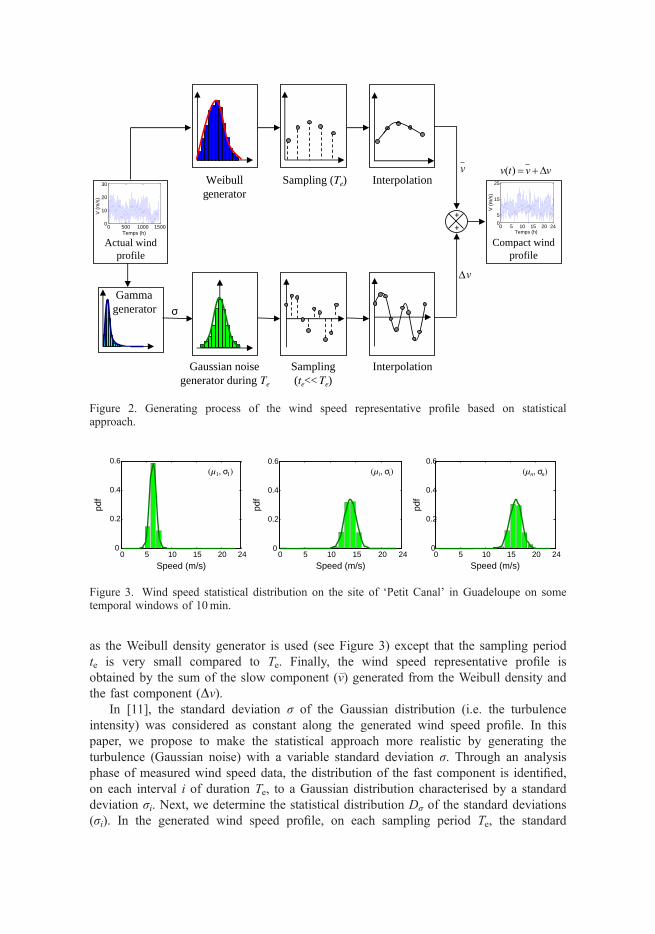
as the Weibull density generator is used (see Figure 3) except that the sampling periodte is very small compared to Te. Finally, the wind speed representative profile isobtained by the sum of the slow component (�v) generated from the Weibull density andthe fast component (Dv).
In [11], the standard deviation σ of the Gaussian distribution (i.e. the turbulenceintensity) was considered as constant along the generated wind speed profile. In thispaper, we propose to make the statistical approach more realistic by generating theturbulence (Gaussian noise) with a variable standard deviation σ. Through an analysisphase of measured wind speed data, the distribution of the fast component is identified,on each interval i of duration Te, to a Gaussian distribution characterised by a standarddeviation σi. Next, we determine the statistical distribution Dσ of the standard deviations(σi). In the generated wind speed profile, on each sampling period Te, the standard
Gaussian noise generator during Te
InterpolationSampling(te<< Te)
Actual windprofile
Sampling (Te) Interpolation
Compact windprofile
Weibullgenerator
Gamma generator
v
v
0 5 10 15 20 2405
15
25
Temps (h)
V (m
/s)
0 500 1000 15000
10
20
30
Temps (h)
V (m
/s)
Figure 2. Generating process of the wind speed representative profile based on statisticalapproach.
0 5 10 15 20 240
0.2
0.4
0.6
0 5 10 15 20 240
0.2
0.4
0.6
0 5 10 15 20 240
0.2
0.4
0.6
Speed (m/s)Speed (m/s)
Speed (m/s)
Figure 3. Wind speed statistical distribution on the site of ‘Petit Canal’ in Guadeloupe on sometemporal windows of 10min.

deviation of the Gaussian noise is determined from a random number generator basedon the same probability density as the statistical distribution of standard deviations (Dσ)(see Figure 2).
The Figure 3 shows the wind speed statistical distribution on the site of ‘PetitCanal’ in Guadeloupe on some temporal windows of 10min. We verify that thesedistributions follow a Gaussian function with parameters ( μ, σ), centred on the meanvalue of the slow component of the wind speed over the temporal window of 10min:
f ðvÞ ¼ 1
rffiffiffiffiffiffi2p
p exp �ðv� lÞ22r2
!ð3Þ
The statistical distribution Dσ of standard deviations (σi) on two months of windspeed measurements on the site of ‘Petit Canal’ is given by the histogram of Figure 4.This distribution is identified from a standard least mean square method with a Gammadensity with α= 7.9 and β= 11.3 as parameters. The corresponding probability density f(σ) is given by Equation (4).[20]
f ðrÞ ¼ ba
CðaÞ ra�1 expð�brÞ ð4Þ
where Г is the Gamma function. The inversion of the cumulative distribution functionassociated with this probability density allows generating the turbulence intensity in thesynthesis process of Figure 2. Three simulation results of the statistical approach for thegeneration of a wind speed profile (12, 24 and 48 h duration) are given in Figure 5(a):these synthesised profiles are representative of two months of wind speed measurementson the site of ‘Petit Canal’. The sampling period of the wind slow component Te is setto 10min and that of the fast dynamics (turbulence) te is fixed to 1 s. Those values arein accordance with the corresponding frequencies issued from the well-known Van derHoven’s spectral distribution.[21,22] We then obtain respectively 72, 144 and 288samples by the Weibull generator (k = 3.03 and c = 10.65) and 600 samples by theGaussian generator for each time interval Te. The Figure 5(b) shows a comparisonbetween the statistical distribution functions ( pdf ) of the generated (12, 24 and 48 h
0 1 2 3 4 50
0.5
1
1.5
1.8
Standard deviation (m/s)
Standard deviations histogramIdentification with a Gammadistribution
Figure 4. Statistical distribution of standard deviations associated with the turbulence.

duration) and original (2months duration) profiles. The more duration increases (thenumber of sample increases), the more generated profile pdf is similar to the referencepdf. We conclude that the statistical approach requires long durations to better representthe actual profile.
Through an analysis of the fast dynamic of the obtained profile, it is shown that thestatistical distribution of some temporal windows of 10min does not exactly follow aGaussian distribution. This difference is due to the strong wind speed variationsbetween two successive samples obtained from the Weibull generator and distant of aperiod Te. This phenomenon modifies the statistical distribution of the fast componentof wind speed (initially a Gaussian distribution). To rectify this problem, one solution isto increase the sampling time of the Weibull generator (for example 5Te instead of Te)
0 2 4 6 8 10 120
5
10
15
20
25
Time (h)
Spee
d (m
/s)
0 5 10 15 20 240
0.02
0.04
0.06
0.08
0.1
0.12
0.14
0.16
Speed (m/s)
Generated profile pdfReference pdf
0 5 10 15 20 240
5
10
15
20
25
Time (h)
Spee
d (m
/s)
0 5 10 15 20 240
0.02
0.04
0.06
0.08
0.1
0.12
0.14
0.16
Speed (m/s)
Generated profile pdfReference pdf
0 10 20 30 40 480
5
10
15
20
25
Time (h)
Spee
d (m
/s)
0 5 10 15 20 240
0.02
0.04
0.06
0.08
0.1
0.12
0.14
0.16
Speed (m/s)
Generated profile pdfReference pdf
(a) Generated profile (b) Statistical distribution functions
Figure 5. Results of the statistical approach for a three time horizon: 12, 24 and 48 h.

in order to enhance the decoupling of slow and fast dynamics. However, this solution islimited in terms of representative profile duration. Indeed, the choice of a samplingperiod multiple of Te increases the generated profile duration and therefore increases thecomputing time of design models, being especially critical in an optimization context.
We present in Figure 6, a simulation of the statistical approach with a samplingperiod of 5Te (the samples obtained by Weibull generator are separated by5Te = 50min). We obtain a profile with a duration of 120 h (5 days) having a statisticaldistribution ( pdf ) very similar to the reference distribution that characterises the twomonths of wind speed measurements on the site of ‘Petit Canal’ (see Figure 6(b)).Furthermore, one can verify that the statistical distribution of the generated fast dynam-ics follows a Gaussian distribution on each temporal window of 10min (see Figure 7).
In conclusion, this statistical approach allows generating wind speed profiles whichare relatively realistic as long as the duration of the synthesised profiles is sufficientlyhigh. However, it does not guarantee to be relevant with regard to the air massacceleration. In other words, no constraints are imposed on the wind speed variationsbetween two successive samples of the random number generators.
3. Compact and representative synthesis approach by EA
In this section, a second approach is proposed for synthesising a compact andrepresentative profile of an actual wind speed profile. This approach consists ingenerating a fictitious wind speed profile by fulfilling some constraints (typically
0 20 40 60 80 100 1200
5
10
15
20
25
Time (h)
Spee
d (m
/s)
0 5 10 15 20 240
0.02
0.04
0.06
0.08
0.1
0.12
Speed (m/s)
Generated profile pdf
Reference pdf
(a) Generated profile (b) Statistical distribution functions
Figure 6. Results of the statistical approach for a time horizon of 120 h.
0 5 10 15 20 240
0.050.1
0.150.2
0.250.3
0.35
Speed (m/s)
0 5 10 15 20 240
0.050.1
0.150.2
0.250.3
0.35
Speed (m/s)pd
f0 5 10 15 20 24
00.050.1
0.150.2
0.250.3
0.35
Speed (m/s)
Figure 7. Wind speed statistical distribution on some temporal windows of 10min of thegenerated profile (120 h).

minimum, maximum and average values, and probability distribution function). Theseconstraints are expressed in terms of target indicators that can be evaluated from a setof actual profiles or from a single reference profile of large duration (for example somemonths/years of data).
3.1. Principle
The synthesis process of compact wind profiles is based on the approach developed in[23] for railway driving missions. It consists in generating a fictitious profile of anyenvironmental variable (e.g. temperature, wind speed, solar irradiation) by fulfillingsome constraints related to the variables (typically minimum, maximum and averagevalues and probability distribution function). These constraints are expressed in termsof target indicators that can be evaluated from a set of real cycles or from a single realcycle of large duration. The fictitious profile is obtained by aggregating elementarypatterns (segments) as shown in Figure 8. Each segment is characterised by itsamplitude ΔSn (ΔSmin ref6ΔSn6ΔSmax ref) and its duration Δtn (06Δtn6Δtcompact). Atime scaling step is performed after the profile generation in order to fulfil the constraintrelated to the time duration, i.e. ΣΔtn=Δtcompact. Finding a compact fictitious profile ofan environmental variable consists in finding all segment parameters so that thegenerated profile fulfils all target indicators on the reduced duration Δtcompact. Thisresults in solving an inverse problem with 2Nm parameters where Nm denotes thenumber of segments in the compact profile. This can be done using EAs [24,25] andespecially with the clearing method [26] well suited to treat this kind of problem withhigh dimensionality and high multimodality.
In addition to the choice of the parameters of each pattern, the EA is encoded sothat the number of segments (Nm) can be itself optimised through a self-adaptiveprocedure.[23] Indeed, contrary to the classical chromosome encoding strategies whichencods the same number of patterns for all individuals in the population (Figure 9(a)), asecond strategy allowing the parallel investigation of signal configurations with distinctnumber of patterns is proposed (Figure 9(b)). It consists in encoding in the chromosomean additional gene representing the number of patterns. This number can vary from 1 toNm max, Nm max denoting the maximum number of patterns. However, it should be notedthat the chromosome is identical for all individuals in the population, containing theparameters associated with Nmmax patterns. Then, only a part of the chromosome isconsidered in the individual decoding according to value of the gene associated with
ttn
Sn
Sn
S1S2
S3
S4
S5
S6S7
t
S
(a) Profile generated by segments (b) Pattern parameters: Sn and tn
Figure 8. Principle of the profile generation.

the number of patterns. The other genes are not expressed and can be considered as‘recessive’. They are not used in the individual decoding but participate to crossoverand mutation operations. Moreover, the EA is implemented using real-encoded decisionvariables, standard binary tournament selection, classical BLX-0.5 crossover [27] withmaximum crossover rate ( pc = 1) and random mutation with probability pm= 1/n wheren denotes the total number of decision variables. The clearing procedure used as nich-ing method is coded with a niche capacity of 1 and with a classical elitism scheme.[26]
The synthesis process of wind speed profile by means of optimization is given inFigure 10. The aim is to minimize the error function ɛ expressed by Equation (5). Thisfunction represents the overall gap between the reference values of specific indicators(Ij ref) from the actual wind speed profile and those of the generated profile (Ij). Theseindicators will be detailed in the following subsection.
e ¼Xj
IjðXÞ � Ij refIj ref
� �2
ð5Þ
3
2
Nbr of patterns
1st pattern parameters
2nd pattern parameters
3rd pattern parameters
4th pattern parameters
…
…
…
…
Nm max pattern parameters
1st pattern parameters
2nd pattern parameters
3rd pattern parameters
Nm pattern parameters
“Dominant genes" “Recessive genes"
(a) Encoding with fixed number of patterns (Nm) (b) Encoding with variable number of patterns (Nm [1, Nm max])
Figure 9. Individual genotype according to the chromosome encoding strategy (with fixed orvariable number of patterns).
Evaluation of indicators
andcontraints
Construction of the S(t)
profile from elementary
patterns
EvolutionaryAlgorithm
1
.
.
.
Nm max
S(t)
Indicators
Contraints
Chromosome X
Ij ref
1
Nm max
tcompact
Figure 10. Synthesis optimization process of wind speed representative profile.

In addition to the error function minimization, it may be necessary to impose someconstraints on the generated profile (minimum and maximum values of standarddeviation). These constraints (Ck) are formulated in terms of inequalities (Ck(X)6 0)and integrated into the error function in the form of penalties:
e ¼Xj
IjðXÞ � Ij refIj ref
� �2
þXk
kk maxð0;CkðXÞÞ2 ð6Þ
where λk is a penalty factor associated to the kth constraint and X denotes an individualchromosome (real encoded vector containing the parameters of the elementary patterns).
3.2. Specific indicators of wind speed
An analysis phase of the wind speed in the temporal and statistical plan allowed us topropose a set of specific indicators related to the main design criteria of wind turbinesystems:
• Maximum speed value: Vmax
This indicator takes account of wind gusts when sizing the wind turbine.
Vmax ¼ maxt2½0 Dtprofile �
V ðtÞ ð7Þ
where Δtprofile denotes the duration of the reference wind profile.
• Average cubic wind speed value: hV3iThe average cubic wind speed value hV3i is used instead of the average wind speedvalue hVi because the power produced by the wind turbine (PWT) is directlyproportional to the cubic wind speed value as shown in Equation (8).
PWT ¼ 1
2qCpSV
3 ð8Þ
where ρ denotes the air density in kgm�3, S indicates the area swept by the windturbine blades in m2, Cp represents the power coefficient defined by the ratio betweenthe power captured by the wind turbine and the initial power of the air mass flowingthrough the area S at the speed V.
• Probability density function: pdfIt is relevant to take account of the wind speed statistical distribution ( pdf ) in the windturbine design. The representative profile to be generated must then fulfil the samestatistical distribution as the actual wind speed measured over a longer duration.
• The wind turbulence: IturbWind turbulence is a crucial phenomenon in the estimation of the wind turbine lifetime(mechanical stress). It is then important to integrate an indicator to characterise theturbulence in the representative temporal profile. We then characterise the wind

turbulence, on each interval i of duration Te = 10min, by the standard deviation σi.[28]We define the turbulence indicator Iturb of the wind profile by the average value ofstandard deviations σi.
Iturb ¼ hrii where i ¼ 1; integer partðDtprofile=TeÞ� � ð9Þ
3.3. Results of the synthesis process of the representative profile
As previously, the reference values of the indicators are determined from two months ofwind speed measurements on the site of ‘Petit Canal’ in Guadeloupe. Nevertheless, thechoice of the representative profile duration is not obvious. Although the specificindicators of wind speed do not impose any minimum duration, the generated profilemust include a sufficient number of samples in order to fulfil the reference statisticaldistribution ( pdfref). The error function to be optimised is given by the followingexpression:
e ¼ VmaxðXÞ � Vmax ref
Vmax ref
� �2
þ hV ðXÞ3i � hV 3irefhV 3iref
!2
þ IturbðXÞ � Iturb refIturb ref
� �2
þ estat ð10Þ
where ɛstat represents the mean square error between the reference statistical distribution(pdfref) and that of the generated profile (pdfgen) evaluated from 20 equal intervals ofwidth Vmax ref/20.
estat ¼ 1
20�X20k¼1
pdfgenðX; kÞ � pdfref ðkÞpdfref ðkÞ
� �2
ð11Þ
The Figure 11 gives a process result of a representative profile with a 3 h duration(compared with the initial duration of two months, i.e. almost 1500 h). The EApopulation size is set to 100 and the generation number is equal to 105. The obtainednumber of elementary patterns (number of segments) is 217.
0 0.5 1 1.5 2 2.5 30
5
10
15
20
25
Time (h)
Spee
d (m
/s)
5 10 15 20 24
0.02
0.04
0.06
0.08
0.1
0.12
Speed (m/s)
Generated profile pdfReference pdf
0
(a) Generated profile (b) Statistical distribution functions
Figure 11. Synthesis process result of representative profile of a 3 h duration.

The characteristics of the generated wind speed profile are given in Table 1. Theobtained results are perfect in the sense of specific indicators while two months of windspeed measurements (�1500 h) are compacted in a ratio 500 (�1500/3).
A second solution to enhance compacity of the generated profile duration is tointegrate the phenomenon of turbulence as a constraint in the synthesis optimizationprocess. Instead of imposing an average standard deviation as turbulence indicator, arange of variation of the standard deviation between a minimum and a maximum valuerespectively σmin and σmax has been considered. The turbulence indicator is no longerrepresented by an optimization criterion but instead by the two constraints σmin andσmax. For two months of wind speed measurements on the site of ‘Petit Canal’, thestandard deviation of wind speed intervals (Te = 10min) varies between σmin = 0.05m s�1
and σmax = 4.9m s�1. An illustration of this solution for one hour generated profileduration is given in Figure 12(a). This wind speed profile is obtained by the concatena-tion of 105 segments. The generation number is equal to 15,000 which onlycorresponds to 5 hours of computation with a standard computer (Core Duo 2 GHz).Note that, despite the complexity of the inverse problem (211 parameters), the EAconverges towards a very convenient solution respecting the constraint related to theturbulence phenomenon. Indeed, the Figure 12(b) shows that the statistical distributionof the generated profile perfectly corresponds with the reference distribution. TheTable 2 also shows the low difference between the reference indicators and thegenerated profile indicators.
Finally, the synthesis approach by EA is very efficient in terms of accuracy andreduction of the real wind speed profile duration. Indeed, two months of wind speedmeasurements are compressed in 1 h only. Consequently, this reduction provides asignificant gain in terms of computing time which is particularly useful in theframework of wind turbine system design by optimization.
Table 1. Comparison of the generated profile indicators to the reference indicators.
Reference indicators Generated profile indicators Error (%)
Vmax (m s�1) 23.1 23.1 0.0hV3i (m3 s�3) 1076 1076 0.0Iturb 0.72 0.74 2.7
0 0.2 0.4 0.6 0.8 10
5
10
15
20
25
Time (h)
Spee
d (m
/s)
0 5 10 15 20 240
0.02
0.04
0.06
0.08
0.1
0.12
0.14
0.16
Speed (m/s)
Generated profile pdf
Reference pdf
(a) Generated profile (b) Statistical distribution functions
Figure 12. Synthesis process result of representative profile of a 1 h duration.

4. Comparison of the two synthesis approaches
In this section, the statistical synthesis approach is compared with the EA-basedsynthesis approach by considering the same conditions in terms of computation timewith the same computer. 5 h of computation time are chosen which corresponds to theconvergence time required for synthesis approach by EA to generate a representativeprofile from two months of wind speed measurements on the site of ‘Petit Canal’ inGuadeloupe. Regarding the statistical synthesis approach, we proceed to generate awind speed profile by successive iterations during 5 h of computation time. At eachiteration, the obtained profile is retained if it improves the same error function ɛ used inthe synthesis approach by EA (see Equation (12)). This error function aims atsimultaneously optimising the maximum wind speed value, the average cubic windspeed value and the statistical distribution. In order to simplify this comparison, theturbulence indicator has not been considered here. The error function evolution over 5 hof computation is given in Figure 13.
e ¼ Vmax � Vmax ref
Vmax ref
� �2
þ hV 3i � hV 3irefhV 3iref
� �2
þ 1
20�X20k¼1
pdf ðkÞ � pdfref ðkÞpdfref ðkÞ
� �2
ð12Þ
The representative profile duration is set to 1 h in the synthesis approach by EA and5 days (120 h) in the statistical synthesis approach. This difference between thedurations of representative profiles is related to the characteristics of each approach.Indeed, the statistical approach is not very relevant with short durations due to lownumber of samples while the synthesis approach by EA allows obtaining short duration
Table 2. Comparison of the generated profile indicators to the reference indicators.
Reference indicators Generated profile indicators Error (%)
Vmax (m s�1) 23.1 23.1 0.0hV3i (m3 s�3) 1076 1078 0.2
0 1 2 3 4 5
10-1
100
Simulation time (h)
Erro
r
Statistical approachEA approach
Figure 13. Error function evolution for the two synthesis approaches.

profiles (1 h). The characteristics of the representative profiles obtained after 5 h ofcomputing time on a standard PC (Core Duo 2 GHz) are given in Figure 14 andTable 3.
The obtained results show that the EA-based synthesis approach provides a betteraccuracy with respect to all indicators. In particular, the statistical distribution of theobtained profile perfectly follows the reference statistical distribution. Converselysignificant differences can be observed in the case of the statistical approach (seeFigure 14). In addition, the synthesis approach by EA leads to more compact durationof the representative profile. Indeed, two months of wind speed measurements are onlyrepresented by a profile of one hour duration.
0 0.2 0.4 0.6 0.8 10
5
10
15
20
25
Time (h)
Spee
d (m
/s)
0 20 40 60 80 100 1200
5
10
15
20
25
Time (h)
Spee
d (m
/s)
0 5 10 15 20 240
0.02
0.04
0.06
0.08
0.1
0.12
0.14
0.16
Speed (m/s)
Generated profile pdf
Reference pdf
0 5 10 15 20 240
0.02
0.04
0.06
0.08
0.1
0.12
0.14
0.16
Speed (m/s)
Generated profile pdfReference pdf
(a) Synthesis approach by EA (b) Statistical Synthesis approach
Figure 14. Comparison of generated profiles by the two synthesis approaches – time series andassociated distributions.
Table 3. Comparison of generated profiles characteristics by the two synthesis approaches.
Vmax (m s�1) hV3i (m3 s�3)
Reference indicators 23.1 1076Generated profile indicatorsEA approach 23.1 1078Statistical approach 22.2 1077
Error (%)EA approach 0 0.2Statistical approach 3.9 0.1

5. Application of the synthesis approach by EA to a stand-alone wind systemhybridised with storage
In this section, the interest of the compact and representative synthesis approach of awind speed profile is illustrated on the sizing of a simple stand-alone system. Thesystem is composed of a given 8 kW passive wind turbine [7,29] hybridised with a leadacid battery pack. The system is supposed to supply a periodic load profile Pload (24 hperiod). The problem here only consists in sizing the battery bank considering a givenwind turbine and a wind farm potential represented by a reference wind profile resultingfrom 200 days of wind speed measurements. Unlike the previous case where theindicators are directly related to the wind speed characteristics, the indicators used inthis application are also related to the sizing constraints on the storage system. Threeparticular indicators are considered: PBTmax, PBTmin and Es which respectively denotethe maximum and the minimum storage powers in the battery and the storage usefulenergy defined by Equation (13).[30] These indicators represent the physical variablesrequired for the battery bank sizing.
The reference values of these indicators are extracted from the simulation of thewind speed actual profile of 200 days duration (see Figures 15 and 16). Note that thereference value of the storage useful energy Esref is defined as follows:
Esref ¼ maxEBTðtÞ �minEBTðtÞ ð13Þ
where EBTðtÞ ¼R t0 PBTðsÞds ¼
R t0 ðPWTðsÞ � PloadðsÞÞds t 2 ½0; 200 days�
PBT, PWT and Pload are respectively the battery power, the power supplied by thewind turbine and the load power.
It should be noted that EBT(t) is a saturated integral with 0 as upper limit so that thebattery storage is only sized in discharge mode to avoid its oversizing during wide chargeperiod (huge winds with reduced load). An additional target indicator is considered totake account of statistic features of the reference wind cycle. We use the cumulativedistribution function cdfref computed from the corresponding probability density functionpdfref related to the reference wind speed behaviour.[31] The pdfref is evaluated from 20equally spaced intervals between 0 and the maximum wind speed value.
Finally, the global error ɛ to be minimised in the synthesis profile process can beexpressed as:
e ¼ PBTmax � PBTmax ref
PBTmax ref
� �2
þ PBTmin � PBTmin ref
PBTmin ref
� �2
þ Es � Es ref
Esref
� �2
þestat ð14Þ
where the statistic error ɛstat denotes the mean squared error between both cdfs relativeto reference and generated wind speed profiles:
estat ¼ 1
20�X20k¼1
cdf ðkÞ � cdfref ðkÞcdfref ðkÞ
� �2
ð15Þ
All ‘ref’ indexed variables are based on the reference wind profile of Figure 16.The inverse problem has been solved with the ‘clearing’ algorithm using a populationsize of 100 individuals and a number of generations of 500,000. Multiple optimization

runs were performed with different compaction time Δtcompact. In particular, theminimum compaction time (i.e. min (Δtcompact)) was determined using dichotomoussearch in order to ensure a global error ɛ less than 10�2. The Table 4 shows the valuesof the global error ɛ vs. the compaction time. It can be seen that the lowest value forΔtcompact ensuring the fulfilment of the target indicators with sufficient accuracy is about10 days. The Figure 17 shows the characteristics of the generated wind profile obtainedfrom the aggregation of 109 elementary segments fulfilling all target indicators. It canbe seen from this figure that the cdf of this compact wind profile closely coincides withthat of the reference wind profile.
Batteries
Actual windprofile (200 days)
Passive windturbine
Load profile
PBTmax ref , PBTmin ref , Esref , cdfref
Extraction of indicators reference values
PBT
PloadPWT
Figure 15. Extraction of indicator reference values from the actual wind speed profile of200 days duration.
0 50 100 150 2000
10
20
30
Spee
d (m
/s)
0 50 100 150 200
0
20
40
PBT
(kW
)
0 50 100 150 200-40
-20
0
Time (day)
E (k
Wh)
Figure 16. Actual reference wind speed profile and corresponding storage power/energy.

The Table 5 compares the values of the target indicators related to the battery sizingfor the reference and the fictitious profile generated with the ‘clearing’ algorithm. Agood agreement between those values indicates that the compact wind profile wouldlead to the same battery sizing as the reference wind profile with longer duration(200 days).
6. Conclusion
In this paper, two different approaches have been developed for compacting wind speedprofiles. The first concerns a purely statistical approach based on random numbergenerators with probability density functions derived from the statistical distribution ofactual wind speed data. The authors have proposed a more realistic consideration of thefast wind speed dynamics representative of the turbulence phenomenon.
In a second approach, a synthesis process of representative wind speed profile ofreduced duration has been developed. This process is based on the aggregation orconcatenation of elementary patterns which the number and the parameters aredetermined by an EA optimization. It allows synthesising a fictive and compact windspeed profile which verifies a set of pertinent indicators with regard to design criteria
Table 4. Influence of Δtcompact on the global error ɛ.
Δtcompact (days) 40 20 10 5
Global error ɛ ≈8� 10�3 ≈9� 10�3 ≈9� 10�3 ≈7� 10�2
0 2 4 6 8 100
5
10
15
20
25
30
Time (days)
Spee
d (m
/s)
0 5 10 15 20 240
0.2
0.4
0.6
0.8
1
Speed (m/s)cd
f
Generated profile cdfReference cdf
(a) Generated profile (b) Cumulative distribution functions
Figure 17. Synthesis process result of representative profile over a 10 days duration.
Table 5. Target indicators of the generated wind speed profile.
Reference indicators Generated profile indicators Error (%)
PBTmax (kW) 30 30 0.0PBTmin (kW) �5.88 �5.82 0.1Es (kWh) 32.36 32.4 0.12

and constraints. Two months of wind speed measurements are compressed in only 1 h.Consequently, this reduction provides a significant gain in terms of computing time inthe framework of the optimization process of wind turbines.
Then, a comparative study of the two synthesis approaches for the same computingcost has been established. Note that the synthesis approach by EA gives the advantageof a more compact duration of representative profiles.
Finally, the synthesis approach by EAwas applied for sizing a stand-alone hybrid sys-tem based on wind turbine and batteries as storage elements. The indicators considered inthis application are related to storage device features. The synthesis approach by EA hasproven its effectiveness in reducing 200 days of wind speed measurements in only10 days, allowing sizing the storage system with a significant gain in terms of computingtime in the framework of the optimization process. Note that this synthesis approach isvery generic, which can exceed the particular field of wind turbines design to be appliedin the whole range electrical engineering applications and even beyond, by processingany types of environmental variables (wind speed but also temperature, sun irradiation,etc.) or for example of railway driving profiles as proposed in [23].
AcknowledgmentThe authors would like to thank the GRER (Renewable Energy Research Group – AntillesGuyane) for availability of wind speed sequences measured at the site of ‘Petit Canal’ inGuadeloupe.
References
[1] Feijoo AE, Cidras J, Dornelas JLG. Wind speed simulation in wind farms for steady-statesecurity assessment of electrical power systems. IEEE Trans. Energy Convers.1999;14:1582–1588.
[2] Dobigeon N, Tourneret JY. Joint segmentation of wind speed and direction using ahierarchical model. Comput. Stat. Data Anal. 2007;51:5603–5621.
[3] Mohandes M, Rehman S, Halawani TO. A neural networks approach for wind speedprediction. Renewable Energy J. 1998;13:345–354.
[4] Damousis IG, Alexiadis MC, Theocharis JB, Dokopoulos PS. A fuzzy model for wind speedprediction and power generation in wind parks using spatial correlation. IEEE Trans. EnergyConvers. 2004;19:352–361.
[5] Slootweg JG, de Haan SWH, Polinder H, Kling WL. General model for representingvariable speed wind turbines in power system dynamics simulations. IEEE Trans. PowerSyst. 2003;18:144–151.
[6] Roboam X, editor. Integrated design by optimization of electrical energy systems. London(UK): Wiley ISTE; 2012. Available from: http://www.eu.wiley.com/WileyCDA/WileyTitle/productCd-1848213891.html
[7] Tran DH, Sareni B, Roboam X. Integrated optimal design of a passive wind turbine system:an experimental validation. IEEE Trans. Sustainable Energy. 2010;1:48–56.
[8] Abdelli A, Sareni B, Roboam X. Model simplification and optimization of a passive windturbine generator. Renewable Energy J. 2009;34:2640–2650.
[9] Calif R, Blonbou R, Deshaies B. Wind velocity measurements analysis for time scales smal-ler than 1 hour: application to wind energy forecasting. Proceedings of the 24th AIAA/ASME Wind Energy Symposium, Reno (NV); 2005.

[10] Calif R, Emilion R, Soubdhan T. Classification of wind speed distributions using a mixtureof Dirichlet distributions. Renewable Energy. 2011;36:3091–3097.
[11] Roboam X, Abdelli A, Sareni B. Optimization of a passive small wind turbine based onmixed Weibull-turbulence statistics of wind. Québec: Electrimacs; 2008.
[12] Sayood K. Introduction to data compression. 4th ed. Waltham (MA): Morgan-Kaufmann;2012.
[13] Joseph P, Hennessey J. Some aspects of wind power statistics. J. Appl. Meteorol. Climatol.1977;16:119–128.
[14] Celik AN. A statistical analysis of wind power density based on the Weibull and Rayleighmodels at southern region of Turkey. Renewable Energy. 2003;29:593–604.
[15] Weisser D. A wind energy analysis of Grenada: an estimation using the ‘Weibull’ densityfunction. Renewable Energy. 2003;28:1803–1812.
[16] Keller JK. Simulation of wind with ‘K’ parameter. Wind Eng. 1992;16:307–312.[17] Carta JA, Ramírez P, Velázquez S. A review of wind speed probability distributions used in
wind energy analysis: case studies in the Canary Islands. Renew. Sustain. Energy Rev.2009;13:933–955.
[18] Straroon DA, Stengelz RF. Stochastic prediction techniques for wind shear hazardassessment. J. Guid. Control Dyn. 1990;15:1224–1229.
[19] Nichita C, Luca D, Dakyo B, Ceanga E. Large band simulation of the wind speed for realtime wind turbine simulators. IEEE Trans. Energy Convers. 2002;17:523–529.
[20] Law AM, Kelton WD. Simulation modeling and analysis. 2nd ed. New York: McGraw Hill;1991.
[21] Van der Hoven I. Power spectrum of horizontal wind speed in the frequency range from0.0007 to 900 cycles per hour. J. Atmos. Sci. 1957;14:160–164.
[22] Bianchi FD, Batista H, Mantz RJ. Wind turbine control systems: principle, modeling andgain scheduling design, advances in industrial control series. London: Springer-Verlag; 2010.
[23] Jaafar A, Sareni B, Roboam X. Signal synthesis by means of evolutionary algorithms.Inverse Prob. Sci. Eng. 2012;20:93–104.
[24] Schwefel HP. Evolution and optimum seeking. New York (NY): Wiley; 1995.[25] Sareni B, Krähenbühl L. Fitness sharing and niching methods revisited. IEEE Trans. Evol.
Comput. 1998;3:97–106.[26] Petrowski A. A clearing procedure as a niching method for genetic algorithms. Proceedings
of the IEEE International Conference on Evolutionary Computation; 1996; Nagoya, Japan.[27] Eshelman LJ, Schaffer JD. Real-coded genetic algorithms and interval schemata. In Whitley
D, editor. Foundations of genetic algorithms II; 1993. P. 187–202.[28] Frandsen S, Thogersen M. Integrated fatigue loading for wind turbines in wind farms by
combining ambient turbulence and wakes. J. Wind Eng. 1999;23:327–339.[29] Belouda M, Belhadj J, Sareni B, Roboam X. Battery sizing for a stand-alone passive wind
system using statistical techniques. 8th IEEE International Multi-conference on Systems,Signals and Devices (SSD); 2011; Hammamet, Tunisia.
[30] Belouda M, Belhadj J, Sareni B, Roboam X, Jaafar A. Synthesis of a compact wind profileusing evolutionary algorithms for wind turbine system with storage. 16th IEEEMediterranean Electrotechnical Conference; 2012; Medina, Yasmine Hammamet-Tunisia.
[31] Bagul AD, Salameh ZM, Borowy BS. Sizing of a stand-alone hybrid wind-photovoltaic sys-tem using a three-event probability density approximation. Sol. Energy. 1996;56:323–335.