examination of potential benefits of an energy … the western interconnection m. milligan and k....
TRANSCRIPT

NREL is a national laboratory of the U.S. Department of Energy, Office of Energy Efficiency & Renewable Energy, operated by the Alliance for Sustainable Energy, LLC.
Contract No. DE-AC36-08GO28308
Examination of Potential Benefits of an Energy Imbalance Market in the Western Interconnection M. Milligan and K. Clark National Renewable Energy Laboratory
J. King and B. Kirby Consultants
T. Guo and G. Liu Energy Exemplar
Technical Report NREL/TP-5500-57115 March 2013

NREL is a national laboratory of the U.S. Department of Energy, Office of Energy Efficiency & Renewable Energy, operated by the Alliance for Sustainable Energy, LLC.
National Renewable Energy Laboratory 15013 Denver West Parkway Golden, Colorado 80401 303-275-3000 • www.nrel.gov
Contract No. DE-AC36-08GO28308
Examination of Potential Benefits of an Energy Imbalance Market in the Western Interconnection M. Milligan and K. Clark National Renewable Energy Laboratory
J. King and B. Kirby Consultants
T. Guo and G. Liu Energy Exemplar
Prepared under Task Nos. DP08.7010, SM12.2011
Technical Report NREL/TP-5500-57115 March 2013

NOTICE
This report was prepared as an account of work sponsored by an agency of the United States government. Neither the United States government nor any agency thereof, nor any of their employees, makes any warranty, express or implied, or assumes any legal liability or responsibility for the accuracy, completeness, or usefulness of any information, apparatus, product, or process disclosed, or represents that its use would not infringe privately owned rights. Reference herein to any specific commercial product, process, or service by trade name, trademark, manufacturer, or otherwise does not necessarily constitute or imply its endorsement, recommendation, or favoring by the United States government or any agency thereof. The views and opinions of authors expressed herein do not necessarily state or reflect those of the United States government or any agency thereof.
Available electronically at http://www.osti.gov/bridge
Available for a processing fee to U.S. Department of Energy and its contractors, in paper, from:
U.S. Department of Energy Office of Scientific and Technical Information P.O. Box 62 Oak Ridge, TN 37831-0062 phone: 865.576.8401 fax: 865.576.5728 email: mailto:[email protected]
Available for sale to the public, in paper, from:
U.S. Department of Commerce National Technical Information Service 5285 Port Royal Road Springfield, VA 22161 phone: 800.553.6847 fax: 703.605.6900 email: [email protected] online ordering: http://www.ntis.gov/help/ordermethods.aspx
Cover Photos: (left to right) PIX 16416, PIX 17423, PIX 16560, PIX 17613, PIX 17436, PIX 17721
Printed on paper containing at least 50% wastepaper, including 10% post consumer waste.

iii
Acknowledgments The National Renewable Energy Laboratory gratefully acknowledges the support of Larry Mansueti, Jon Worthington, and the Department of Energy Office of Electricity Delivery and Energy Reliability as well as Kevin Lynn, Venkat Banunarayanan, and the U.S. Department of Energy Solar Energy Technologies Office SunShot Intitative for funding this work.
The National Renewable Energy Laboratory also thanks Victoria Ravenscroft previously of the Western Interstate Energy Board of the Western Governors’ Association, Doug Larson of the Western Interstate Energy Board of the Western Governors’ Association, and the Public Utility Commissions Energy Imbalance Market task force for their organizational support and assistance in engaging stakeholders.
And many thanks to the members of the technical review committee for their insightful comments and assistance. Participation in the technical review committee does not imply agreement with the project findings. The technical review committee included:
• Jamie Austin, Pacificorp • Venkat Banunarayanan, U.S. Department of Energy Solar Program • Steve Beuning, Xcel Energy • Patrick Damiano, Columbia Grid • Jeanine Divis, Arizona Public Service • Brent Guyer, Avista Corp. • Paul Humberson, Western Area Power Authority • Brendan Kirby, Consultant • JJ Jamieson, Versify Solutions • Rebecca Johnson, Colorado Public Utilities Commission • Gary Lawson, Sacramento Municipal Utility District • Michael McGowan, Northwestern Energy • Michelle Mizumori, Western Electricity Coordinating Council • Carl Monroe, Southwest Power Pool • Tony Montoya, Western Area Power Authority • Jack Moore, Energy and Environmental Economics • Arne Olson, Energy and Environmental Economics • Jim Price, California Independent System Operator • David Schiada, Southern California Edison • Justin Thompson, Arizona Public Service.

iv
Finally, the National Renewable Energy Laboratory thanks the many members of the broader stakeholder community for their comments on the interim presentations and draft report. Comments provided by reviewers represent the opinions of the individual reviewers, and their participation does not imply agreement with the project findings. Reviewers of the interim presentations and draft report included:
• Elise Caplan, American Public Power Association • David Crowell, Salt River Project • Jeanine Divis, Arizona Public Service for the Southwest Variable Energy Resource
Initiative • Kris Mayes, Kris Mayes Law Firm for Interstate Renewable Energy Council • Clint Kalich, Avista Corp. • Brendan Kirby, consultant • Jimmy Lindsay, Renewable Northwest Project • Paul McCurley, National Rural Electric Cooperative Association • Nancy Norris, Powerex • Gregory Miller, Public Service of New Mexico • Jim Price, California Independent System Operator • Ken Rose, independent consultant • Kevin Smith, Braun Blaising McLaughlin & Smith for Sacramento Municipal Utility
District and the Balancing Authority of Northern California • John Stout, Mariner Consulting Services • Brian Whalen, NV Energy • Tom Veselka, Argonne National Laboratory for Western Area Power Administration.
The National Renewable Energy Laboratory regrets any inadvertent omission of any project participants and contributors.

v
List of Acronyms ACE area control error ADI ACE Diversity Interchange AESO Alberta Electric System Operator AVA Avista AZPS Arizona Public Service BA balancing authority BAA balancing authority area BANC Balancing Area of Northern California BAU business as usual BCTC British Columbia Transmission Corp. BPA Bonneville Power Administration CAISO California Independent System Operator CC combined cycle CFE Comision Federal de Electricidad CHPD Public Utility District No. 1 of Chelan County CSP concentrating solar power CT combustion turbine DC direct current DCOPF direct current optimal power flow DOPD Public Utility District No. 1 of Douglas County E3 Energy and Environmental Economics EIM energy imbalance market EPE El Paso Electric FRCC Florida Reliability Coordinating Council GCPD Public Utility District No. 1 of Grant County GW gigawatt GWh gigawatt-hour IID Imperial Irrigation District IPC Idaho Power Corp. ISO independent system operator ISO-NE ISO New England ITAP Intra-Hour Transaction Accelerator Platform LADWP Los Angeles Department of Water and Power LMP locational marginal pricing MAGIC Magic Valley MRO Midwest Reliability Organization NEVP Nevada Power NPCC Northwest Power Coordinating Council NREL National Renewable Energy Laboratory NWE Northwest Energy NWMT Northwest Montana NWPP Northwest Power Pool PACE Pacificorp East PACE_ID Pacificorp Idaho PACE_UT Pacificorp Utah

vi
PACE_WY Pacificorp Wyoming PACW Pacificorp West PC planning case PG&E Pacific Gas and Electric PGN Portland General Electric PNM Public Service Company of New Mexico PMA power marketing administration PSCO Public Service Company of Colorado PSE Puget Sound Energy PV photovoltaic(s) PUD public utility district RFC ReliabilityFirst Corp. SCE Southern California Edison SCED security-constrained economic dispatch SCL Seattle City Light SCUC security-constrained unit commitment SDGE San Diego Gas and Electric SERC Southeastern Electric Reliability Council SMUD Sacramento Municipal Utility District SPP Southwest Power Pool SPPC Sierra Pacific Power Co. SRP Salt River Project SUNY State University of New York SVERI Southwest Variable Energy Resource Initiative TEP Tucson Electric Power TEPPC Transmission Expansion Planning and Policy Committee TES thermal energy storage TID Turlock Irrigation District TPWR Tacoma Power TRE Texas Reliability Entity TREAS Treasure Valley WACM Western Area Colorado Missouri WALC Western Area Lower Colorado WAPA Western Area Power Administration WAUM Western Area Upper Missouri WECC Western Electricity Coordinating Council WWSIS Western Wind and Solar Integration Study

vii
Executive Summary In the Western Interconnection, there is significant interest in improving approaches to wide-area coordinated operations of the bulk electric power system, in part because of the increasing penetration of variable generation. These approaches include, but are not limited to, area control error pooling (area control error diversity interchange), advanced approaches to dynamic scheduling (dynamic scheduling system), and an Intra-Hour Transaction Accelerator Platform. They also include more recent analysis and proposals from the Northwest Power Pool Market Assessment and Coordination Committee and the Southwest Variable Energy Resource Initiative. In addition, an energy imbalance market (EIM) has been proposed as a way to improve wide-area coordination. This study focused on that approach alone, with the goal of identifying the potential benefits of an EIM in the year 2020.
The primary objective of an EIM is to quickly dispatch generation to meet load across a broad geographic region. The economic dispatch of the EIM would operate every 5 minutes, allowing for a more economic balancing than would result if regulating resources were used for all imbalance inside the hour. Part of the generation-load imbalance that needs to be addressed derives from the variability and uncertainty associated with wind and solar generation. An EIM takes advantage of the reduction in wind and solar generation variability that is achieved via the geographic diversity inherent across a wide area. An EIM also allows a broader geographic range of generation resources to contribute to the economic balancing of generation and load. Thus, the EIM is intended to provide better generation-load balancing by being both big and fast. Participation in the EIM would be voluntary—as determined by each balancing authority and the generation resources within each balancing authority area.
A series of studies, largely requested or encouraged by Western state electricity regulators and other state officials, has focused on the potential impact of an EIM. In 2011, the Western Electricity Coordinating Council (WECC) evaluated a proposed EIM in partnership with Energy and Environmental Economics (E3). The study was based on the Transmission Expansion Planning and Policy Committee (TEPPC) Planning Case 0 (PC0), which included annual energy penetrations of 8% wind and 3% solar in the year 2020.i A large industry group provided guidance. The study evaluated only the electricity production cost savings of the EIM based on hourly time-step simulations (i.e., capital and other costs were excluded). Societal benefits—those accruing to the entire interconnection—were defined as the reduction in electricity production cost because of the EIM.
In early 2012, a group of public utility commissioners in the West expressed interest in additional analyses of the potential operational benefits of an EIM. The Public Utility Commissions Energy Imbalance Market (PUC EIM) Group,ii facilitated by the Western Interstate Energy Board, was formed. The PUC EIM Group asked the U.S. Department of Energy’s Office of Electricity Delivery and Energy Reliability to fund the National Renewable Energy Laboratory to perform the work.
i The wind and solar penetration levels in WECC’s TEPPC PC0 were estimates of the generation needed to meet individual state renewable portfolio standard requirements. See http://www.wecc.biz/library/StudyReport/Documents/ Assumptions%20Matrix%20for%20the%202020%20TEPPC%20Dataset.pdf. ii Additional information about the PUC EIM Group can be found at http://www.westgov.org/PUCeim.

viii
Four key factors bound the scope of this study.
1. This analysis was designed as an extension of the WECC-E3 study and, therefore, adopted all the assumptions of that study.
2. This study used an electricity production simulation model, PLEXOS, with 10-minute time-step capability, rather than the hourly time-step of the WECC-E3 study, to better represent the 5-minute dispatch interval of the proposed EIM.
3. This study was limited to an evaluation of the potential operational savings of the EIM and did not include an assessment of EIM implementation or other costs.
4. This study evaluated the potential benefits of an EIM with full participation and an EIM with a reduced level of participation and included selected sensitivity analyses.
Decision-makers may want to consider additional factors outside the scope of this report to determine whether participation in an EIM would be advantageous for their individual balancing authority areas.
Study Limitations Modeling any large system, especially one with the physical characteristics and existing market relationships of the Western Interconnection, is complex. In addition, all studies have limitations and are subject to input data assumptions and modeling approximations. For example, this study examines only the potential production cost savings of an EIM for a specific set of study cases based on the TEPPC PC0 model and assumptions. Limitations include the lack of:
• Bilateral power purchase agreement data • Detailed operational constraints in the hydro generation models • Capability to simultaneously model different dispatch intervals in different balancing
authority areas • Real-time quick-start generation commitment procedures.
There are also uncertainties surrounding:
• Future cooperation and/or subhourly dispatch across the interconnection • The amount and location of variable generation • Transmission system additions • Generation additions and retirements • Gas and coal prices • The EIM participation level.
Lack of contractual data has a significant impact on the commitment and dispatch performed by the production simulation software. Without such data, the software develops a minimum production cost commitment and dispatch, subject only to generating unit operating limits, transmission path ratings, and other performance constraints. Therefore, all individual balancing authority area benefits should be considered rough estimates.

ix
Today’s Western Grid Operation The Western Interconnection, shown as part of the overall U.S. power system in Figure i, is composed of more than 30 balancing authorities. Superimposed on this structure are other levels of coordination, such as reserve-sharing groups that coordinate contingency reserve obligations, not shown on the map. There are also several subregional transmission planning groups—such as the group formed by Columbia Grid, Northern Tier Transmission Group, and WestConnect—that coordinate transmission plans.
Source: North American Electric Reliability Corp.
Figure i. North American Electric Reliability Corp. regions and balancing authorities
Unit commitment and economic dispatch are not performed uniformly across the West; however, the objectives are the same. The process of committing generating units and dispatching their output optimizes for the least-cost generation dispatch to meet load, given the various physical, contractual, and institutional constraints inherent in any electric power system.
In general, each balancing authority performs its own unit commitment the day before real-time operation. On the day of real-time operation, balancing authorities dispatch the committed generation to meet the actual load in a number of ways. California and Alberta have large independent system operators with centrally organized electricity markets that include fast (e.g., 5-minute) economic dispatch. Other balancing authorities that own generation can dispatch units within the hour, either systematically (e.g., every 15 or 30 minutes) or on an as-needed basis. Still

x
other balancing authorities may use self-schedules from independent generation owners and bilateral agreements for energy exchange on an hourly basis. Such hourly interchange schedules typically operate with a 20-minute period at the top of the hour to allow units to move to their new operating points. However, there are exceptions. For example, Bonneville Power Administration and the California Independent System Operator are running field trials of shorter interchange intervals. And, as noted above, there are other efforts to better coordinate operations across wider areas.
What Is the Proposed EIM? The primary objective of the proposed EIM is to quickly dispatch generation to meet load across a broad geographic region. The EIM would perform a regional security-constrained economic dispatch,iii for all participating generation, every 5 minutes solely to manage imbalances between generation and load and relieve transmission constraints. The EIM assumes each participant will continue to provide sufficient resources to cover its own obligations (i.e., commit sufficient generation to meet load, reserve requirements, and interchange agreements). EIM power flows would receive the lowest transmission service priority. Therefore, EIM flows would not displace reserved transmission service.
Unlike other regional markets in which transmission service for market delivery is provided under a regional network service tariff, EIM flows would be accompanied by an imputed service compensation after the fact to participating transmission providers. At this stage of development, the specific terms for the transmission service revenue target and revenue allocation among participating transmission providers have not been established.
Figure ii illustrates the timeline of the security-constrained economic dispatch of an EIM. It would take 10 minutes from the time a system snapshot is taken until units have moved to their new set point. This process would repeat every 5 minutes.
Figure ii. EIM schedule for calculating dispatch set points
and moving generation within 10 minutes
iii Security-constrained economic dispatch is defined as “the operation of generation facilities to produce energy at the lowest cost to reliably serve consumers, recognizing any operation limits of generation and transmission facilities.” See http://www.ferc.gov/industries/electric/indus-act/joint-boards/south-recom.pdf.

xi
Study Methods The data requirements for this study included load, wind power, and solar power profiles and forecasts. The 2006 time series of load, wind power, and solar power profiles were used so common weather impacts would be maintained. The 2006 data were mapped to the simulation year 2020. WECC provided hourly load profile data projected for 2020 based on the 2006 load shapes, from which Pacific Northwest National Laboratory synthesized 10-minute load profiles. Wind data were obtained from NREL’s Western Wind and Solar Integration Study database (3TIER 2010). Solar data were developed by NREL. As noted previously, the variable renewable scenarioiv was defined by WECC TEPPC PC0 and includes approximately 8% wind and 3% solar penetration (by energy) in the Western Interconnection.
There were two primary analytical components to this study. First, a statistical data analysis was performed to determine the flexibility reserves required to meet the variability and uncertainty of wind and solar generation. Second, production simulation analysis was performed to evaluate grid operation over a full year for various study scenarios to identify potential EIM operational savings benefits.
Flexibility reserves are a new type of reserve specifically designed to address the variability and uncertainty of wind and solar generation. They are separate and distinct from the reserves the power system already requires to address load variability and contingencies (Ela et al. 2011). Similar resources can fulfill both needs and come from the same resource pool (e.g., conventional generation and responsive load), but this analysis does not use contingency or other existing reserves to provide flexibility reserves. Flexibility reserves are in addition to those reserves.
Flexibility reserves are a function of the time-synchronized expected variability of wind and solar power, which is, in turn, a function of wind or solar output. For example, if wind power output is at or near maximum, then there is relatively little variability and, therefore, relatively small flexibility reserve requirements. Conversely, if wind power output is in the middle of the operating range, then its variability is higher, and the flexibility reserve requirements are higher. The flexibility reserve requirements are therefore calculated for every hour of the year for each study scenario.
For this study, the flexibility reserve requirements were divided into three classes based on the type of resources required to fulfill them:
1. Regulation covers fast changes of wind and solar power within the forecast interval. These changes can be up or down and happen minute-to-minute. This class of flexibility reserve covers minute-to-minute wind and solar variability and short-term forecast errors. Regulation requires resources on automatic generation control.
2. Spinning reserves cover larger, less-frequent variations primarily caused by longer-term forecast errors. Spinning reserves are provided by resources (generation and responsive load) that are spinning and can fully respond within 10 minutes. These resources do not necessarily require automatic generation control.
iv This study analyzed only variable renewable generation (i.e., wind and solar). Other renewable generation (e.g., geothermal, hydro, and biomass) are included in TEPPC PC0 but were not germane to this analysis.

xii
3. Non-spinning and supplemental reserves cover large, slower-moving, infrequent events such as unforecasted ramping events. Non-spinning reserves can be available within 10 minutes and can come from quick-start resources and responsive load. Supplemental reserves can be made available within 30 minutes.
Because of software limitations, flexibility regulation and flexibility spinning reserves are represented as additional spinning reserves in the simulations. Non-spinning reserves could not be represented.
Production simulation analysis simulates actual bulk power system operations using time-synchronized load, wind, and solar data for each balancing authority; the associated flexibility reserve requirements; existing contingency reserve requirements; the TEPPC PC0 transmission system topology and constraints (e.g., path limits and nomograms); and operating characteristics for each unit in the generation portfolio. The simulation software solves the cost-minimization problem while respecting various input constraints. PLEXOS production simulation software was used for this study because of its hourly and subhourly simulation time-step capability. The subhourly capability was used with a 10-minute time-step to match the load, wind, and solar input data resolution and approximate the EIM’s dispatch interval of 5 minutes.
Production simulations produce an enormous volume of output data, which include generator commitment and dispatch, emissions, costs, and transmission path flows for each time-step of the year. Production costs are a key simulation output and consist of the fuel and variable operations and maintenance costs for the generation fleet. Fixed costs (e.g., power plant construction costs) are not included.
To evaluate the potential operational savings of an EIM, two simulations were required: a business-as-usual (BAU) case and an EIM case. The societal (total throughout the West) savings from the EIM is the difference in production cost between these two cases, as shown in Figure iii.
Figure iii. EIM benefit formula
Additional analysis was required to determine how these societal benefits should flow to individual EIM participants. In the WECC-E3 study, a method was developed to evaluate how those benefits would be allocated. This method was referred to as the Benefits Allocation Roadmap. The calculations are based on the specific results from the production cost modeling and additional information, such as total load served and generation owned, supplied by the participants. Individual balancing authorities can potentially refine the allocation results by accounting for confidential bilateral and other contracts not included in the production simulations.
The study examined several scenarios representing different EIM participation levels, hourly and 10-minute BAU cases, alternative natural gas prices, and reduced flexibility reserve requirements.
EIM
Benefit Production cost of BAU
Production cost of EIM

xiii
Flexibility Reserve Reduction Flexibility reserve requirements can be reduced by an EIM. Figure iv shows the average flex reserve requirements under alternative EIM scenarios and dispatch interval/forecast lockdown assumptions. The right panel shows the flex reserves calculated for a range of BAU dispatch intervals (10–60 minutes) and forecast lockdown periods (10–40 minutes). The forecast lockdown period is the time between the last available forecast and actual operation. The middle panel shows the impact of three subregional EIMs on flexibility reserve requirements. The left panel shows the impact of a full EIM on flexibility reserve requirements. Flexibility reserve requirements decrease with shorter dispatch interval/forecast lockdown times and with larger EIMs.
Figure iv. Effect of dispatch interval and aggregation size on reserve requirements

xiv
Faster Dispatch Faster dispatch intervals for generating plants can reduce total production costs. Today, it is common in the West for dispatch and interchange functions to be performed hourly. However, some areas are experimenting with subhourly dispatch, and Federal Energy Regulatory Commission Order 764 stipulates that 15-minute schedules be offered. Figure v shows the total production cost difference—approximately $1.3 billion—between an hourly BAU case and a 10-minute BAU case. (Note that the y-axis minimum on this and subsequent figures is not zero. The total y-axis range remains the same across all figures for ease of comparison.)
Figure v. Potential impact of BAU assumptions on total production cost
19,000
20,000
21,000
22,000
Tota
l Pro
duct
ion
Cost
($M
)
Hourly BAU10-minute BAU
~ $1.3 B

xv
Full-Footprint EIM Full EIM participation can reduce total production costs. The total production costs for the hourly and 10-minute BAU cases and the associated 10-minute full-EIM cases are shown in Figure vi. Note that each EIM case uses the unit commitment developed by its associated BAU case. Full EIM participation includes all balancing authority areas in the Western Interconnection except the California and Alberta independent system operators.
The full EIM with the hourly BAU commitment results in a savings of $294 million/year over the hourly BAU case. The full EIM with the 10-minute BAU commitment results in a savings of $146 million/year over the 10-minute BAU case.
Figure vi. Full-footprint EIM results under alternative BAU and commitment assumptions
19,000
20,000
21,000
22,000
Hourly 10-minute
Tota
l Pro
duct
ion
Cost
($M
)
BAU
Full EIM~ $300 M
~ $150 M
~ $1.3 B

xvi
Reduced EIM Participation The production cost savings from an EIM can vary with participation level. The total production costs for the hourly and 10-minute BAU cases and the associated 10-minute reduced-participation EIM cases are shown in Figure vii. Note that each EIM case uses the unit commitment developed by its associated BAU case. For the reduced-EIM participation cases, which were requested by the PUC EIM Group, Bonneville Power Administration and two of the three Western Area Power Administration balancing authority areas are omitted. Several public utility districts, along with Seattle City Light and Tacoma Power, are embedded in Bonneville Power Administration and, therefore, were also removed from EIM participation.
The reduced EIM with the hourly BAU commitment results in a savings of $276 million/year over the hourly BAU case. The reduced EIM with the 10-minute BAU commitment results in a savings of $95 million/year over the 10-minute BAU case. These savings are less than those achieved with full EIM participation.
Figure vii. Reduced-footprint EIM benefits for hourly and 10-minute unit commitment
19,000
20,000
21,000
22,000
Hourly 10-minute
Tota
l Pro
duct
ion
Cost
($M
)
BAU
Reduced Participation EIM
~ $300 M
~ $100 M
~ $1.3 B

xvii
Low Natural Gas Prices The production cost savings from an EIM can also vary with natural gas price. A nominal natural gas benchmark price of $7.28/MMBtu, consistent with the TEPPC 2020 planning case, was used for most of the analysis. By today’s standards, this is a high price. Therefore, a lower price of $4.50/MMBtu was used to evaluate the impact of lower natural gas prices on EIM benefits. The latest Energy Information Administration forecast shows approximately $4.60/MMBtu (2011 dollars) natural gas prices for the electric power sector from 2016 on (U.S. Energy Information Administration 2012). The total production costs for the hourly BAU case and the associated 10-minute full-EIM case with the lower gas price are shown in Figure viii. The full EIM benefit is $281 million/year, which is a slight reduction from the $294 million/year of operational benefit achieved at the higher gas price.
Figure viii. Comparison of EIM benefits using the hourly BAU/EIM and $4.50/MMBtu natural gas
15,000
16,000
17,000
18,000
Tota
l Pro
duct
ion
Cost
($M
)
Hourly BAU with lower gas price
Full EIM with lower gas price
~ $300 M

xviii
Summary of West-Wide Results This study shows an annual West-wide operating benefit of between $146 million and $294 million for the EIM with full participation. An additional benefit of approximately $1.3 billion is associated with moving from an hourly dispatch interval to a 10-minute dispatch interval. Therefore, the total benefit of a faster dispatch interval and shared flexibility reserves could be as high as $1.46 billion. Summaries of these West-wide results are shown in Figure ix and Table i.
Figure ix. Comparison of West-wide EIM benefits
Table i. West-Wide Annual EIM Benefits
Case Annual Savings
($ Millions) Full EIM with hourly BAU commitment compared with hourly BAU 294 Full EIM with 10-minute BAU commitment compared with 10-minute BAU 146 Reduced EIM with hourly BAU commitment compared with hourly BAU 275 Reduced EIM with 10-minute BAU commitment compared with 10-minute BAU 95 Lower-gas-price, full EIM with hourly BAU commitment compared with hourly BAU 281 10-minute BAU compared with hourly BAU 1,312
294 275 281
146 95
1,312
-
200
400
600
800
1,000
1,200
1,400
Full EIM ReducedParticipation EIM
Full EIM at LowerGas Price
Faster Dispatch
Tota
l Pro
duct
ion
Cost
Sav
ings
($M
) Hourly
10-minute
From hourly to 10-minute

xix
The largest benefit ($1.3 billion/year) is achieved by moving from hourly to 10-minute dispatch across the entire Western Interconnection. This faster dispatch is a main component of the EIM. The other component is sharing flexibility reserves across a wide area to take advantage of the reduced wind and solar variability associated with geographic diversity. Therefore, the 10-minute BAU could be considered a step along the path to the full-EIM implementation in which fast dispatch is adopted before the rest of the EIM. The potential benefits associated with the rest of the EIM range from $95 million/year to $294 million/year, depending on the BAU dispatch interval, EIM participation level, and natural gas price assumption. The lower estimate with full-EIM participation ($146 million/year) is based on the assumption that all balancing authority areas practice 10-minute dispatch in the BAU case. The upper estimate with full-EIM participation ($300 million/year) is based on the assumption of hourly dispatch in the BAU case. With a lower level of participation, the annual benefit of the EIM ranges from $95 million to $275 million. The potential benefits of all EIM variations compared with an hourly BAU case are approximately $300 million/year.
Individual Balancing Authority Area Results EIM benefits were allocated to individual balancing authority areas by calculating an adjusted production cost for each balancing authority area. This method has its roots in work performed at the Southwest Power Pool (2005) and in the Eastern Wind Integration and Transmission Study (EnerNex Corp. 2010) and was refined by E3 (2011). It takes into account not only the change in production cost but also the changes in imports and exports and calculates an adjusted production cost accordingly. The adjusted production cost decreased in the majority (21 of 29) of the balancing authority areas, showing a potential EIM benefit. Conversely, eight balancing authority areas showed an increase in adjusted production cost for a potential EIM cost.
Lack of contractual data among generators, transmission providers, and load serving-entities has a significant impact on the commitment and dispatch performed by the production simulation software. Without such data, which can show how much spare transmission capacity is available, the software develops a minimum production cost commitment and dispatch, subject only to generating unit operating limits, transmission path ratings, and other performance constraints. The EIM modeled in this study assumes that physically available transmission capacity can be used for EIM transactions but with a lower priority than all other transmission uses. Physical limitations on transmission use are included in the modeling; however, contractual information is not. Therefore, all individual balancing authority area benefits should be considered rough estimates.
Individual balancing authority areas could refine the allocation results by accounting for confidential bilateral and other contractual mechanisms. For example, if a balancing authority area has contractual obligations to sell a given amount of energy during a year at a specified price, the revenue from those sales will not be affected by potential EIM transactions. Likewise, if a balancing authority area holds contracts for purchases at a specified price, the EIM would have no impact on that cost.
Future Work As in any complex modeling and analysis of future conditions, additional questions surfaced as the work progressed. Therefore, additional analysis on the following topics is recommended:

xx
• Power purchase agreements, if they could be made available
• Alternative nonvariable generation mixes, including alternative assumptions regarding coal plant retirements
• Alternative wind and solar energy penetration levels and locations
• Alternative EIM participation scenarios
• Multiple EIMs
• Alternative fuel price and/or emissions prices and regulations
• Alternative seams management with EIM nonparticipants to explore nonparticipant benefits
• Broader use of subhourly scheduling (e.g., Joint Initiative Intra-Hour Transaction Accelerator Platform, Federal Energy Regulatory Commission Order 764)
• Alternative future transmission projects
• Improved generation modeling (e.g., unit-specific rather than generic data).
This project pushed the state of the art for electricity production simulation modeling to the limit, evaluated potential EIM benefits under a range of conditions, and identified areas for future research. Further analysis and model refinements are recommended to more fully assess the impact of the proposed EIM on the Western Interconnection. Such an effort could provide additional insight into the modeling of a large, complex system such as the Western Interconnection and the potential benefits of various operational changes.

xxi
Table of Contents 1 Introduction ........................................................................................................................................... 1
1.1 Today’s Western Grid Operations ................................................................................................... 2 1.2 Why an EIM? ................................................................................................................................... 3 1.3 Overview of the Proposed EIM ....................................................................................................... 3 1.4 Prior EIM Analyses.......................................................................................................................... 6
2 Study Approach .................................................................................................................................... 7
2.1 Input Data ........................................................................................................................................ 9 2.2 Reserves Calculation Method ........................................................................................................ 16 2.3 Modeling Limitations..................................................................................................................... 22 2.4 Study Cases .................................................................................................................................... 24 2.5 Production Simulation Model ........................................................................................................ 32
3 Impact of an EIM ................................................................................................................................. 44
3.1 Reserve Calculation Results .......................................................................................................... 44 3.2 PLEXOS Model Alignment to WECC-E3 Results ........................................................................ 48 3.3 Full EIM ......................................................................................................................................... 53 3.4 Gas Price Sensitivity ...................................................................................................................... 60 3.5 Reduced-Participation EIM Sensitivity ......................................................................................... 63 3.6 Additional Sensitivity Cases .......................................................................................................... 66 3.7 Comparison of Hourly and 10-Minute BAU Cases ....................................................................... 68
4 Allocation of EIM Benefits to Participants ....................................................................................... 71
4.1 Allocation Method ......................................................................................................................... 71 4.2 Allocation of Benefits for EIM Under Hourly BAU ..................................................................... 73 4.3 Allocation of Benefits for EIM Compared With the 10-Minute BAU .......................................... 82
5 Conclusions ........................................................................................................................................ 88
6 References .......................................................................................................................................... 91

xxii
List of Figures Figure 1. Operation timeline for the EIM toolkit ..........................................................................4 Figure 2. EIM schedule for calculating dispatch set points and moving generation within
10 minutes ......................................................................................................................5 Figure 3. Cycle of calculations and unit ramping .........................................................................5 Figure 4. The EIM footprint, which effectively pools variability .................................................6 Figure 5. Overview of the study approach ....................................................................................7 Figure 6. EIM benefit formula ......................................................................................................8 Figure 7. Example correction of the third-day anomaly in the Western Wind and Solar
Integration Study wind data set ....................................................................................12 Figure 8. Actual load, hourly average, and interpolated load for 2009 .......................................15 Figure 9. Imposing the 2009 load variability on the 2020 interpolated load ..............................15 Figure 10. Example persistence forecast for 10-minute dispatch .................................................18 Figure 11. Short-term forecast error standard deviation as a function of wind production
level ..............................................................................................................................18 Figure 12. Hour-ahead forecast error standard deviation as a function of wind production
level ..............................................................................................................................20 Figure 13. Effect of hourly dispatch and 40-minute forecast lead on forecast error .....................21 Figure 14. Effect of dispatch interval and aggregation size on reserve requirements ...................22 Figure 15. PLEXOS security-constrained unit commitment and economic dispatch algorithm ..33 Figure 16. Hydro dispatch comparison between this study and TEPPC results ...........................40 Figure 17. WECC BAA map with subregional groups .................................................................43 Figure 18. Reserve requirements for sample BA for three study scenarios ..................................45 Figure 19. Flex reserve duration plot for sample BA for three study scenarios ............................46 Figure 20. Flex reserve requirements duration for full-EIM footprint for three study
scenarios .......................................................................................................................47 Figure 21. Flex reserve requirements as a function of dispatch interval and forecast lead
time ..............................................................................................................................48 Figure 22. Comparison of total energy production between PLEXOS and GridView in the
BAU alignment case ....................................................................................................49 Figure 23. Comparison of total production cost between PLEXOS and GridView in the
BAU alignment case ....................................................................................................50 Figure 24. Comparison of total energy production between PLEXOS and GridView for the
full-EIM alignment case ..............................................................................................51 Figure 25. Comparison of total production cost between PLEXOS and GridView for the
full-EIM alignment case ..............................................................................................52 Figure 26. Comparison of total production cost for the full-EIM participation and the hourly
dispatched BAU ...........................................................................................................54 Figure 27. Comparison of annual energy production by generation class in the hourly
dispatched BAU and full EIM cases ............................................................................56 Figure 28. Comparison of total production cost for the full-EIM participation and the
10-minute dispatched BAU..........................................................................................58 Figure 29. Comparison of annual energy production by generation class in the 10-minute
dispatched BAU and full-EIM cases ............................................................................59 Figure 30. Comparison of total production cost by generation class for reduced-gas-price
hourly BAU and EIM cases .........................................................................................61

xxiii
Figure 31. Comparison of generation for reduced-gas-price cases ...............................................62 Figure 32. LMP map for hourly BAU case ...................................................................................77 Figure 33. LMP map for full-EIM case with hourly BAU unit commitment ...............................79 Figure 34. LMP map of LMP changes from hourly BAU to full EIM with hourly unit
commitment .................................................................................................................80 Figure 35. LMP map for 10-minute BAU case .............................................................................84 Figure 36. LMP map for full-EIM case with 10-minute BAU unit commitment .........................86 Figure 37. LMP map of LMP changes from 10-minute BAU to full EIM with 10-minute
unit commitment ..........................................................................................................87

xxiv
List of Tables Table 1. BAAs Defined for This Study .......................................................................................10 Table 2. Variable Generation Penetration (by Energy) for Each BAA .......................................11 Table 3. Case-Naming Convention .............................................................................................25 Table 4. Summary of Study Cases ..............................................................................................31 Table 5. Order of Constraint Relaxation .....................................................................................34 Table 6. Nomograms That Are Enforced ....................................................................................36 Table 7. Hurdle Rates Between BAAs ........................................................................................37 Table 8. Regional Coal Prices .....................................................................................................39 Table 9. Hydro Energy Represented by Each Type of Model ....................................................39 Table 10. Hoover Hydro Power Plant Joint Ownership ................................................................41 Table 11. Colstrip Thermal Power Plant Joint Ownership ............................................................41 Table 12. BAAs Defined for This Study .......................................................................................42 Table 13. Annual Summary of Flex Reserve Requirements for Sample BA for Three Study
Scenarios .......................................................................................................................45 Table 14. Summary of Flex Reserves Requirements for the Full EIM Footprint for Three
Study Scenarios .............................................................................................................46 Table 15. Energy Production by Generation Class for the BAU Alignment Case .......................49 Table 16. Production Cost by Generation Class for the BAU Alignment Case ............................50 Table 17. Energy Production by Generation Class for the Full-EIM Alignment Case ................51 Table 18. Production Costs by Generation Class for the Full-EIM Alignment Case ...................52 Table 19. EIM Production Cost Savings Compared With BAU Alignment Case .......................53 Table 20. Production Cost and Savings for Full EIM Over Hourly Dispatched BAU ................55 Table 21. Generation by Resource Type for the Hourly Dispatched BAU and
Full-EIM Cases ..............................................................................................................56 Table 22. Change in Emissions for Hourly Dispatched BAU and Full-EIM Case ......................57 Table 23. Production Costs and Savings for Full EIM Over 10-Minute Dispatched BAU .........58 Table 24. Energy Production by Generation Class for the 10-Minute Dispatched BAU and
Full-EIM Cases ..............................................................................................................59 Table 25. Change in Emissions for 10-Minute Dispatch BAU and Full EIM .............................60 Table 26. Production Costs and Savings for Full EIM Over Hourly Dispatched BAU With
Low Gas Prices ..............................................................................................................61 Table 27. Energy Production by Generation Class for Full EIM Over Hourly Dispatched
BAU With Low Gas Prices ...........................................................................................62 Table 28. Change in Emissions for Low-Gas-Price Sensitivity Cases .........................................63 Table 29. Production Cost and Savings by Generation Class for Reduced-Participation EIM
Over Hourly Dispatched BAU ......................................................................................64 Table 30. Annual Energy Production by Generation Class for Reduced-Participation EIM
Compared With Hourly Dispatched BAU .....................................................................64 Table 31. Change in Emissions for Hourly Dispatch BAU and Reduced-Participation EIM ......65 Table 32. Production Cost and Changes for Reduced-Participation EIM and 10-Minute
Dispatched BAU ............................................................................................................65 Table 33. Change in Emissions for 10-Minute Dispatch BAU and Reduced-Participation
EIM ................................................................................................................................66 Table 34. Effect of Reduced Flex Reserve Requirements on Production Cost .............................67

xxv
Table 35. Comparison of Production Costs for 1-Hour Time-Step Simulation Versus 10-Minute Time-Step Simulation of Full EIM ..............................................................68
Table 36. Comparison of Production Costs and Savings by Generation Class for 1-Hour and 10-Minute Dispatched BAU Cases ...............................................................................69
Table 37. Total Energy Production by Generation Class for 1-Hour and 10-Minute Dispatched BAU Cases .................................................................................................69
Table 38. Savings Associated With Fast Dispatch and EIM .........................................................70 Table 39. Approximate Production Savings Associated With Faster Dispatch and EIM ............70 Table 40. Allocation of EIM Benefits (With the Hourly BAU Unit Commitment) to EIM
Participants ....................................................................................................................74 Table 41. Allocation of EIM Benefits (With the Hourly BAU Unit Commitment) to EIM
Nonparticipants .............................................................................................................76 Table 42. Average Weighted LMP for Hourly BAU Case ...........................................................78 Table 43. Average Weighted LMP for Full-EIM Case With Hourly BAU Unit Commitment ...79 Table 44. Average Weighted LMP Changes From Hourly BAU to Full EIM With Hourly
Unit Commitment ..........................................................................................................81 Table 45. Allocation of EIM Benefits (With the 10-Minute BAU Unit Commitment) to EIM
Participants ....................................................................................................................83 Table 46. Allocation of EIM Benefits (With the 10-Minute BAU Unit Commitment) to EIM
Nonparticipants .............................................................................................................84 Table 47. Average Weighted LMP for 10-Minute BAU Case ......................................................85 Table 48. Average Weighted LMP for Full-EIM Case With 10-Minute BAU Unit
Commitment ..................................................................................................................86 Table 49. Average Load-Weighted LMP Changes From 10-Minute BAU to Full EIM With
10-Minute Unit Commitment ........................................................................................88 Table 50. Summary of EIM Savings .............................................................................................89

xxvi
List of Equations Equation 1. Calculation of short-term wind standard deviation ................................................19 Equation 2. Calculation of regulation flexibility reserve requirement ......................................19 Equation 3. Sample calculation of hour-ahead wind standard deviation ..................................20 Equation 4. Calculation of spinning flexibility reserve requirement ........................................20 Equation 5. Calculation of non-spinning flexibility reserve requirement .................................21

1
1 Introduction In early 2012, a group of public utility commissions in the West expressed interest in additional analysis of an energy imbalance market (EIM) through an ad hoc group formed under the auspices of the Western Governors’ Association’s Western Interstate Energy Board. In turn, that group asked the U.S. Department of Energy to fund the National Renewable Energy Laboratory (NREL) to conduct such analysis, which culminated in this report. This study extends prior work but leans heavily on the assumptions in the Western Electricity Coordinating Council (WECC) and Energy and Environmental Economics (E3) studies (2011b and 2011c), which, in turn, used the assumptions of the WECC Transmission Expansion Planning and Policy Committee (TEPPC) Planning Case 0 (PC0) for the year 2020.
This study focuses on the potential operational benefits of an EIM in 2020 by using production simulation software to simulate future scenarios. Production simulations determine operating costs, which include fuel, variable operating and maintenance costs, startup costs, and other variable costs. The capital costs of generation and transmission infrastructure, the costs of implementing an EIM (e.g., hardware, software, and communications), and any other direct or indirect costs of an EIM, which may or may not be significant, are not included. Additional detail on the limitations of production simulation model accuracy is provided in Section 2.3. Modeling any large system, especially one with the physical characteristics and existing market relationships of the Western Interconnection, is complex and difficult to capture appropriately. Therefore, the results of this study must be interpreted as one possible outcome, not as a definitive forecast.
This study evaluates potential EIM benefits across the Western Interconnection (societal benefits) and on a balancing authority area-by-balancing authority area (BAA) basis. It explores:
• The benefit of an EIM using 10-minute economic dispatch • Alternative business-as-usual (BAU) cases (one assuming hourly dispatch and the other
assuming 10-minute dispatch) • Alternative EIM participation levels • Alternative flexibility reserve requirements • Alternative natural gas prices.
Three potential operational benefits of the proposed EIM are:
1. The larger electrical footprint results in the reduction of variability and uncertainty in load and solar and wind energy because of increased geographic diversity.
2. The larger footprint allows access to a wider selection of generation, which can result in more cost-effective dispatch.
3. Five-minute dispatch allows for economic adjustments of generation at the time they are needed, which allows ramping to be distributed among more generators and across the hour. General operating practice today in the West constrains ramping to the 20-minute window surrounding the top of the hour, though that may change with Federal Energy Regulatory Commission Order 764.

2
A detailed analysis of the ramping and flexibility reserve implications of several configurations of an EIM is provided in an earlier study (King et al. 2012). This report builds on that work and uses the flexibility reserve calculations to perform a full security-constrained unit commitment and economic dispatch to provide insight into the potential operational benefit of an EIM under alternative participation levels.
1.1 Today’s Western Grid Operations The Western Interconnection is composed of approximately 30 BAAs—most of which do not participate in centrally organized electricity markets that perform economic dispatch on 5- or 10-minute time-steps. The exceptions are market areas in California and Alberta that are full-fledged independent system operators (ISOs) and not the focus of this study. The nonmarket areas of the Western Interconnection do have some market mechanisms, primarily bilateral, that are used by many entities on a regular basis. Much of the interchange energy is exchanged via long-term bilateral contracts and delivered in hourly blocks, which corresponds to the general practice of hourly interchange between balancing authority areas.
Security-constrained economic dispatch (SCED) is not performed uniformly in each Western BAA, just as it is not uniform among regional transmission organizations and ISOs. Balancing authorities (BAs) that own generation can dispatch units within the hour, either systematically or on an as-needed basis. An example of this is Public Service Company of Colorado. Conversely, some BAs do not have the institutional means to request dispatch service from units that are electrically within the BAA but not owned by the BA. One example of this is Bonneville Power Administration (BPA), which can control hydro generation subject to physical and environmental constraints but is unable to access thermal generation within its BAA on a subhourly basis.
Interchange schedules typically operate hourly, with a 20-minute period at the top of the hour in which units move to their new operating points. BPA and California Independent System Operator (CAISO) recently began a 30-minute scheduling field trial with the objective of demonstrating the benefit of faster scheduling steps to help manage wind variability and uncertainty surrounding large wind exports. The initiative spreads ramping more evenly across the hour instead of restricting all ramping activity to the top of the hour.
Other mechanisms allow for similar schedule adjustments within the hour. As part of their Joint Initiative, WestConnect, Columbia Grid, and Northern Tier Transmission Group defined the Intra-Hour Transaction Accelerator Platform (ITAP), which allows for bilateral, on-demand schedule changes on the half-hour. Subscribers to ITAP can create a schedule modification with short notice once a counterparty is identified and agrees to the change. Other aspects of the Joint Initiative include a dynamic scheduling system, which allows participants to create a dynamic schedule on short notice, and the area control error (ACE) Diversity Interchange (ADI), which nets regulation across the participating BAAs.

3
More recently, the Northwest Power Pool began a Market Assessment and Coordination Committee Initiative1 to analyze (1) regulation sharing, (2) expanded use of an ITAP platform, (3) dynamic scheduling, (4) intra-hour pre-scheduling, (5) flexible bilateral contracts, and (6) a potential EIM in the Northwest Power Pool footprint. Even more recently, seven utilities in the Southwest formed the Southwest Variable Energy Resource Initiative.
In June 2012, the Federal Energy Regulatory Commission issued Order 764, which requires, among other things, that transmission operators offer 15-minute scheduling. Because this ruling has not yet been implemented in Western BAAs, it is not clear whether it will induce sufficient counterparties, including wind and solar generation owners, to change scheduling practice from 1-hour blocks to 15-minute schedules. However, some entities in the West believe that, in the future, 15-minute schedules will be the norm.
1.2 Why an EIM? As penetrations of variable generation increase, there is interest in the West in exploring options to efficiently manage it. There are many possible options, including those described above. Outside of the organized markets of California and Alberta, there are no regional transmission operators in the West. However, the WECC Seams Issues Subcommittee proposed in 2010 an EIM similar to the energy imbalance service adopted by the Southwest Power Pool (SPP).
1.3 Overview of the Proposed EIM2 The EIM uses SCED to provide two functions:
• Balancing service This service redispatches generation every 5 minutes to maintain balance between generation and load. For deliveries scheduled in advance, the effect is that the market supplies deviations from schedules in generator output and errors in load schedules.
• Congestion redispatch service This service redispatches generation to relieve overload constraints on the grid. Information provided to the EIM from the enhanced curtailment calculator ensures correct allocation of the costs of redispatch.
An enhanced curtailment calculator, which allocates transmission service curtailments based on service priority for power flow impacts on the grid, would evaluate flows and pass relevant curtailment information to the EIM.
Federal Energy Regulatory Commission pro forma tariff schedules 4 (energy imbalance) and 9 (generation imbalance) provide the approach used by the WECC BAs for balancing services. The proposed EIM replaces part of the BA services and results in a “virtual consolidation” because of a wide-area SCED that covers imbalances. The congestion redispatch service is new to the nonmarket portions of the Western Interconnection.
1 See http://www.westgov.org/PUCeim/meetings/present/nwpp.pdf. 2 This section is adapted from (E3 2011b)..

4
The EIM design includes a feature different from most regional markets in the United States in which internal resources are subject to a “must offer” requirement. Instead, the default operating assumption is that each market participant provides sufficient resources to cover its own obligations (as is the case today) and the regional economic dispatch is provided by any resource that voluntarily offers responsive capability and is cleared by the SCED process. Most transmission service deliveries would continue to use traditional reserved transmission service. The EIM, however, would not use pre-reserved transmission. Instead, the EIM flow would receive the lowest transmission service curtailment priority. By this mechanism, EIM flows would not displace reserved transmission service.
Unlike other regional markets in which transmission service for market delivery is provided under a regional network service tariff, the EIM flows would be accompanied by an imputed service compensation after the fact to participating transmission providers. At this stage of development of the efficient dispatch toolkit, the specific terms for the transmission service revenue target and revenue allocation among participating transmission providers have not been established.
The EIM function adds operational steps to the practices of the Western Interconnection. Functionally, the operating steps for the proposed EIM track closely with the operating process established in the SPP in its Energy Imbalance Service market. Figure 1 illustrates the timeline of the proposed efficient dispatch toolkit.
Figure 1. Operation timeline for the EIM toolkit
Schedule Day - Ahead and up to 30 Minutes Prior to Operating Hour
Real - Time Dispatch Post - Operating
Time
Forecast and unit commit
Generators self - schedule
Generators voluntarily submit offers
Demand-side management resources voluntarily submit offers
Prepare and finalize pre - dispatch schedules
Perform security - constrained economic dispatch to keep balance
Provide redispatch if any congestion occurs
Send dispatch set points to generators
Coordinate any contingency reserve deployments with EIM dispatch
Market Participant : EIM Market Operator
Gather meter data to support settlements
Provide settlement statement and invoices
Transmission Provider
Provide meter data to support settlements

5
Figure 2 shows the sequence of taking the system data, calculating the expected conditions and required set points for the next interval, communicating those set points to generators and responsive loads, and ensuring responsive resources move to the new set points—all in 10 minutes.
Figure 2. EIM schedule for calculating dispatch set points
and moving generation within 10 minutes
Figure 3 shows how continually repeating the process shown in Figure 2 results in meeting a new system dispatch point every 5 minutes based on information that is only 10 minutes old.
Figure 3. Cycle of calculations and unit ramping

6
The EIM would effectively implement some aspects of a virtual BAA across all or some of the Western Interconnection. California and Alberta would not be included because they already have centrally organized energy markets. Imbalances would be netted out, much as they would be in a single BAA. As proposed, the EIM does not result in a coordinated unit commitment, nor does it pool regulation, which remains a service at the local BA level. However, the netting of energy imbalance—which includes impacts of load, solar, and wind energy—is expected to be significant. Figure 4 illustrates the concept, with each of the small bubbles representing a single BAA. The arrows between the BAAs indicate bilateral energy flows that would still occur. Under an EIM, however, only the net imbalance of the EIM footprint must be managed. This results in less net variability within the local BAAs and less ramping across the footprint.
Figure 4. The EIM footprint, which effectively pools variability
1.4 Prior EIM Analyses There have been other analyses of a proposed Western EIM.
NREL examined the ramping and flexibility reserve implications of an EIM using a 30% wind energy penetration from the Western Wind and Solar Integration Study (King et al. 2011) and performed a follow-up study using data from WECC’s PC0 with 8% wind energy and 3% solar energy (King et al. 2012). A simplistic analysis, using representative pricing for the various types of flexibility reserves, provided a rough estimate of the reserve deployment savings.
WECC commissioned E3 to undertake a production simulation analysis of the proposed EIM. NREL provided the chronological flexibility reserves to E3, and these reserves were modeled as a constraint in the GridView model (E3 2011). The WECC-E3 study found the benefit of the EIM to be $141.4 million, assuming full participation from all nonmarket areas of the West. This study also found that removing Pacific Northwest, BC Hydro, and Western Area Power Administration (WAPA) from the EIM reduced the total benefit to $54 million. Full coordination with CAISO had an estimated benefit of $182 million.
EIM Footprint
EIM Tool: SCED
Intra-hour variability is captured and allocated in real time within the entire region, limited by the physical capability of the wires. Diversity benefit
reduces operating costs for balancing

7
Some entities performed follow-up analyses of the WECC-E3 study, but these are generally not publically available.
2 Study Approach Although greater detail is presented later, this overview provides perspective on the extensive analysis and modeling performed for this project.
The original EIM benefits study, undertaken by E3 on behalf of WECC, was built on TEPPC PC0. PC0 was developed by various WECC stakeholders and includes future trajectories for generation and transmission build-out, plant retirements, and wind-solar energy siting and penetration. The wind-solar energy build-out used in this study is thus a product of the TEPPC process, which resulted in the location of potential wind and solar plants in the BAAs of the Western Interconnection. Ten-minute wind and solar energy production models were developed at NREL and based on various weather system models.
The analysis in this study required several steps, as shown in Figure 5. Generally, the analysis was divided into (1) data analysis, including the development of flexibility reserve requirements, and (2) production simulation modeling. These are represented by the two columns in the figure.
Figure 5. Overview of the study approach
Historical wind and solar data
Statistical analysis
Equations that predict next-period variability based on current values of
wind and solar Analysis data for study , wind and solar profiles
Hourly reserve time series synchronized to load , wind, and solar
Production cost modeling GridView and PLEXOS
Production modeling results analysis, including production cost savings
and BAA benefits
Definition of flex reserve sharing areas ( e . g ., BAA or EIM )
NREL Reserves Analysis WECC - E 3 and NREL - Benefits Studies

8
Production simulation models, such as PLEXOS, calculate power system operating costs, which include fuel, variable operating and maintenance costs, startup costs, and other variable costs. The capital costs of generation and transmission infrastructure, the costs of implementing an EIM (e.g., hardware, software, and communications), and any other direct or indirect costs of an EIM are not included. These models solve a cost-minimization problem, subject to the large number of physical and institutional constraints of the power system.
Before the simulation tool, PLEXOS, was run, the flexibility reserve requirements were calculated from the wind and solar power time series data. This flex reserve, which is a relatively new concept, is separate and distinct from contingency reserve and is based on the variability and uncertainty of the wind/solar generation. Flexibility reserves are also a function of geographic aggregation and the dispatch time-step. The process is described in more detail in Section 2.2, but it essentially resulted in hourly or 10-minute reserve requirements for flex regulation and flex spin, which were then input to PLEXOS. For the BAU cases, the process was repeated for every BAA. For the EIM cases, it was performed for the specific EIM participation level under study. The current practices for holding and using contingency reserves are not affected by these flexibility reserves, and contingency reserves cannot be called on to help manage the wind/solar power variability or uncertainty.
Once the flexibility reserves were input to PLEXOS, a day-ahead, security-constrained unit commitment (SCUC) and SCED were calculated for the entire Western Interconnection. This effort used wind and solar power forecasts much as they would be used in actual unit commitment decisions. However, units committed day-ahead cannot generally be de-committed, which reflects actual constraints on these units. Finally, a real-time economic dispatch that used all the information from the prior commitment was run. In real time, “actual” wind and solar power data were used for the dispatch, whereas forecasts of wind and solar power were used in the commitment. This reflects reality. Day-ahead, actual variable generation output is not known with certainty, so real-time operation is constrained by the units that have been previously committed.
This security-constrained unit commitment and economic dispatch simulation minimized operational costs within the given constraints. To evaluate the potential operational savings of the EIM, two simulations were required: a BAU case and an EIM case. The societal (total West) savings from the EIM is the difference in production cost between these two cases, as shown in Figure 6.
Figure 6. EIM benefit formula
The E3 modeling and assumptions were adopted for the NREL study as completely as possible. The E3 study assumed that BAU operation in the Western Interconnection in 2020 would be based on 10-minute dispatch within BAAs and that interchange would continue to occur largely as it does today. The E3 model used an hourly time-step; thus, the equivalent cases in this study also modeled 10-minute dispatch at an hourly time-step. This was done by calculating the flexibility reserves (described below) assuming 10-minute dispatch.
EIM
Benefit Production cost of BAU
Production cost of EIM

9
To answer additional questions about the potential benefit of the EIM, the NREL study added 10-minute dispatch cases with 10-minute time-steps. This 10-minute modeling time-step approximates the operation of the proposed EIM, which would operate on 5-minute time-steps. Thus, there are two types of cases: those run with an hourly time-step to match WECC-E3 and those that are actually simulated with a 10-minute time-step. In the discussion of the 10-minute cases below, it will be necessary to keep in mind these variations.
Further description—of the input data, reserves calculation method, production simulation modeling, and study cases—of the study approach and assumptions is provided in the following sections.
2.1 Input Data The data requirements for this study included load, wind power, and solar power profiles and forecasts. The 2006 time series load, wind power, and solar power profiles were used so common weather impacts would be maintained. The 2006 data were mapped to the simulation year 2020. In this report, “profile” is the actual power production from a wind or solar plant, and “forecast” is the forecasted power production. Both the profiles and forecasts are synthesized and are either hourly or 10-minute values for the entire year, depending on the modeling case in question.
WECC provided hourly load profile data projected for 2020 based on the 2006 load shapes, from which Pacific Northwest National Laboratory synthesized 10-minute load profiles.
Wind data were obtained from NREL’s Western Wind and Solar Integration Study database (3TIER 2010). Solar data were developed by NREL (Orwig et al. 2011). The renewable scenario was defined by the WECC TEPPC PC0 and includes approximately 8% wind and 3% solar penetration (by energy) in the Western Interconnection.
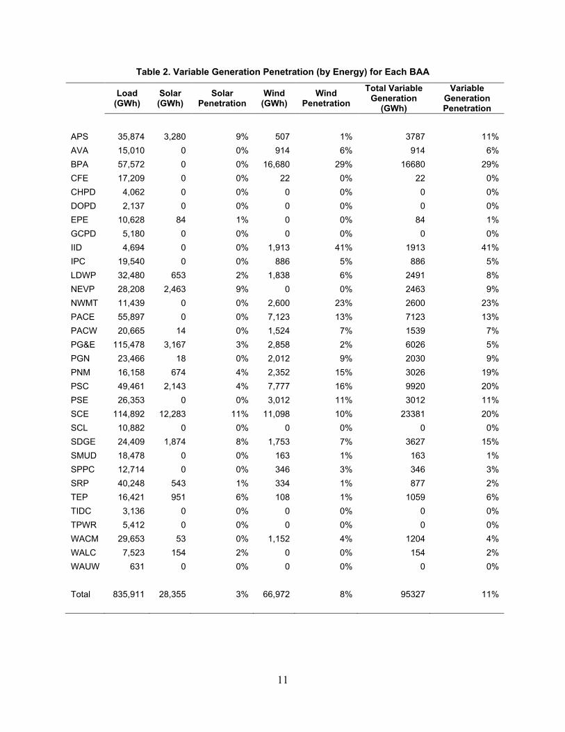
The BAAs were also defined in accordance with the TEPPC case and are shown in Table 1. Table 2 shows the variable generation for each BAA in the study.

10
Table 1. BAAs Defined for This Study
BAAs BAAs Alberta Electric System Operator (AESO) Imperial Irrigation District (IID) Arizona Public Service (AZPS) Los Angeles Department of Water and Power (LADWP) Avista (AVA) Nevada Power (NEVP) Balancing Area of Northern California (BANC) Northern Nevada [Sierra Pacific Power Co. (SPPC)]
Sacramento Municipal Utility District (SMUD) Northwest Energy (NWE) Turlock Irrigation District (TID) Northwest Montana (NWMT)
Bonneville Power Administration (BPA) Western Area Upper Missouri (WAUM) PUD No. 1 of Chelan County (CHPD) Pacificorp East (PACE) PUD No. 1 of Douglas County (DOPD) Pacificorp Idaho (PACE_ID) PUD No. 1 of Grant County (GCPD) Pacificorp Utah (PACE_UT) Seattle City Light (SCL) Pacificorp Wyoming (PACE_WY) Tacoma Power (TPWR) Pacificorp West (PACW)
British Columbia Transmission Corp. (BCTC) or BC Hydro
Portland General Electric (PGN)
California Independent System Operator (CAISO) Public Service Company of Colorado (PSCO) Pacific Gas and Electric (PG&E) Public Service Company of New Mexico (PNM) Southern California Edison (SCE) Puget Sound Energy (PSE) San Diego Gas and Electric (SDGE) Salt River Project (SRP) Comision Federal de Electricidad (CFE) Tucson Electric Power (TEP)
El Paso Electric (EPE) Western Area Colorado Missouri (WACM) Idaho Power Corp. (IPC) Western Area Lower Colorado (WALC)
Far East (FAR EAST) Magic Valley (MAGIC) Treasure Valley (TREAS)
11
Table 2. Variable Generation Penetration (by Energy) for Each BAA
Load (GWh)
Solar (GWh)
Solar Penetration
Wind (GWh)
Wind Penetration
Total Variable Generation
(GWh)
Variable Generation Penetration
APS 35,874 3,280 9% 507 1% 3787 11% AVA 15,010 0 0% 914 6% 914 6% BPA 57,572 0 0% 16,680 29% 16680 29% CFE 17,209 0 0% 22 0% 22 0% CHPD 4,062 0 0% 0 0% 0 0% DOPD 2,137 0 0% 0 0% 0 0% EPE 10,628 84 1% 0 0% 84 1% GCPD 5,180 0 0% 0 0% 0 0% IID 4,694 0 0% 1,913 41% 1913 41% IPC 19,540 0 0% 886 5% 886 5% LDWP 32,480 653 2% 1,838 6% 2491 8% NEVP 28,208 2,463 9% 0 0% 2463 9% NWMT 11,439 0 0% 2,600 23% 2600 23% PACE 55,897 0 0% 7,123 13% 7123 13% PACW 20,665 14 0% 1,524 7% 1539 7% PG&E 115,478 3,167 3% 2,858 2% 6026 5% PGN 23,466 18 0% 2,012 9% 2030 9% PNM 16,158 674 4% 2,352 15% 3026 19% PSC 49,461 2,143 4% 7,777 16% 9920 20% PSE 26,353 0 0% 3,012 11% 3012 11% SCE 114,892 12,283 11% 11,098 10% 23381 20% SCL 10,882 0 0% 0 0% 0 0% SDGE 24,409 1,874 8% 1,753 7% 3627 15% SMUD 18,478 0 0% 163 1% 163 1% SPPC 12,714 0 0% 346 3% 346 3% SRP 40,248 543 1% 334 1% 877 2% TEP 16,421 951 6% 108 1% 1059 6% TIDC 3,136 0 0% 0 0% 0 0% TPWR 5,412 0 0% 0 0% 0 0% WACM 29,653 53 0% 1,152 4% 1204 4% WALC 7,523 154 2% 0 0% 154 2% WAUW 631 0 0% 0 0% 0 0% Total 835,911 28,355 3% 66,972 8% 95327 11%

12
2.1.1 Wind Profiles and Forecasts This study used hourly and 10-minute wind power profiles as well as hourly day-ahead wind forecasts.
As part of the NREL Western Wind and Solar Integration Study, 3TIER Group developed a large wind speed and wind power database (2010). It applied a numerical weather prediction model to re-create the weather and synthesize high-resolution wind speed and power data (every 10 minutes for a 3-year period on a 2-km spatial resolution) across the Western Interconnection. The resulting data set captures the chronological behavior of the wind that would be seen at locations around the West. This high-resolution data set was then used to construct the wind scenario for this study.
The numerical weather prediction model of the Western Interconnection contained geographic and temporal seams that could not be entirely eliminated. This resulted in unrealistic wind energy ramps near the temporal boundaries, which occurred every 3 days. To make the reserves and ramping analysis complete, a continuous annual record was needed, so a method to smooth those ramps below statistical significance was required. To do this, the wind data were analyzed in detail surrounding the anomalies.
The anomalies occurred at approximately the same time, 3 p.m., every third day, starting with the first day of data for all wind plants in the data set. Anomalous data were seen up to 3 hours before this time and 3 three hours after—a side effect of the blending of model runs to mitigate the seams. These anomalous data caused 10-minute ramps more than double that seen anywhere else in the data sets. Figure 7 shows a scatter plot of 10-minute interval changes verses the interval number of a 3-day period. The red dots show where the anomalous data are found. The spikes near 90 on the x-axis show the peak interval changes on the first day. The similar time, 3 p.m., on the second and third days are near 230 and 380 and do not show similar peaks.
Figure 7. Example correction of the third-day anomaly
in the Western Wind and Solar Integration Study wind data set

13
The time range and magnitude of the anomalies were determined. Statistics for similar time periods not affected by the seam were computed. Several moving average filters were designed to push the magnitude of the anomalies below a threshold consistent with statistics from the nonaffected times. The blue dots show the results of the filtering. Although some artifacts of the filtering are observed, the overall shape of the envelope is similar to that of days 2 and 3.
Hourly wind power profiles were developed from the 10-minute profiles by calculating the average of six 10-minute intervals.
Day-ahead, hourly wind power forecasts were also synthesized from a numerical weather prediction model but used a different input data set to ensure independence from the synthesized wind power production profiles. The actual power profiles were driven by the National Center for Environmental Prediction–National Center for Atmospheric Research reanalysis data set, while the forecasts were driven by the Global Forecast System. One consequence of using different data sets was that the total annual energy of the wind forecasts was 10%–20% higher than the total annual energy of the power profiles. Removing this bias is beyond the scope of the current study.
The WECC TEPPC mapped each 2020 PC0 wind plant location to the best available match in this wind database and created aggregate profiles for the work. A total of 29,084 MW of wind plants were included in this case to achieve the 8% (by energy) wind penetration level. The TEPPC wind profiles were disaggregated back to the bus level by Pacific Northwest National Laboratory for use in this study.
2.1.2 Solar Profiles and Forecasts This study used hourly and 10-minute solar power profiles and hourly day-ahead solar forecasts.
Solar power profiles for this study were generated at NREL based on the hourly, satellite-derived data from State University of New York–Clean Power Research and a statistical model to synthesize subhourly variations (Orwig et al. 2011). Power production data were developed for multiple solar technologies, including 50-MW fixed photovoltaics, 50-MW one-axis tracking photovoltaics, and 100-MW concentrating solar power plants with and without thermal energy storage. The data were developed for 1,488 grid locations that correspond to Western Renewable Energy Zones.
Hourly solar power profiles for concentrating solar power were generated using the State University of New York irradiance data and then the System Advisor Model to convert irradiance to power. These 1-hour profiles were interpolated to generate 10-minute concentrating solar power profiles.
For photovoltaics, the procedure for developing the subhourly data included the following steps:
• Classify the cloud regime based on the State University of New York hourly data.
• Use the 1-minute irradiance ground observations to build ramp distributions for each cloud regime.
• Synthesize 1-minute irradiance data for each selected grid cell.

14
• Filter the irradiance data to represent the spatial smoothing.
• Use PVWatts® to convert irradiance to power.
Both the 10-minute and hourly profiles used in this study were generated by averaging the 1-minute data.
Because solar power forecasting is a relatively immature field, the hourly solar power profiles were also used as the day-ahead forecasts. Thus, the solar forecasts were perfect in the unit commitment stage of the production simulations (Section 2.5). Persistence forecasts were used in the calculation of the flexibility reserves (Section 2.2).
The WECC TEPPC mapped each 2020 PC0 solar plant location to the best available match in this solar database and created aggregate profiles for the work. A total of 7023 MW of photovoltaic plants, 1835 MW of concentrating solar power with 6 hours of thermal energy storage, and 5741 MW of concentrating solar power without storage were included in this case to achieve the 3% (by energy) solar penetration level. The TEPPC solar profiles were disaggregated back to the bus level by Pacific Northwest National Laboratory for use in this study.
2.1.3 Load Profiles and Forecasts Because no load data with 10-minute resolution were provided for the study year 2020, these data were generated by Pacific Northwest National Laboratory using a method developed for the WECC Variable Generation Subcommittee study (Samaan 2012). The available load data for the 32 balancing authorities include (1) hourly load for the year 2020 from PROMOD and (2) minute-by-minute load data for the year 2009. Therefore, the following procedures were applied to generate the required load data for the study year 2020. The idea was to impose the minute-to-minute variability of the 2009 load data onto the 2020 data. The procedure was:
• Compute the hourly average load data time series for all 32 BAAs in 2009 with 1-minute resolution.
• Apply MATLAB’s nonlinear interpolation method to obtain a new interpolated load series, as shown in Figure 8.
• Calculate the error between the actual load and interpolated load, normalize it based on the peak load in 2009 for each BAA individually, and scale it by multiplying by the peak load in 2020.
• Interpolate the provided hourly load data in 2020 to obtain 1-minute resolution load data.
• Apply the scaled 2020 error to the 1-minute-resolution 2020 load data to obtain the desired load curves, as shown in Figure 9.
This procedure was applied to the 32 BAAs. For this study, the 1-minute data were averaged to create the needed 10-minute data.

15
Figure 8. Actual load, hourly average, and interpolated load for 2009
Figure 9. Imposing the 2009 load variability on the 2020 interpolated load
Error

16
2.2 Reserves Calculation Method The increased variability and uncertainty from wind and solar power increases the need for operating reserves (e.g., flexible generation and responsive load) that help manage that variability. The additional reserves required are calculated dynamically and are a function of the time-synchronized expected variability of wind and solar power. A method to estimate the requirements for regulation with wind variability was developed in the Eastern Wind Integration and Transmission Study (King et al. 2011, EnerNex Corp. 2010). That method was used to calculate the reserve requirements for this study.
The technique uses statistical analysis of 3 years of simulated historical wind and solar generation to estimate the reserve requirements at periods both faster (to provide regulation) and slower (to follow longer unforecasted changes in variable generation output) than the dispatch interval. These flexibility reserves are in addition to, not instead of, existing contingency reserves and reserve-sharing group arrangements. The flexibility reserves are calculated for each hour of the year to create a dynamic reserve that can be deployed to manage variability and uncertainty over various time scales.
2.2.1 Definition of Flexibility Reserves For this study, the flexibility reserve3 requirements were divided into three classes based on the type of resources required to fulfill them:
1. Regulation covers fast changes of wind and solar power within the forecast interval. These changes can be up or down and happen minute-to-minute. This class of flexibility reserve covers minute-to-minute wind and solar variability and short-term forecast errors. Regulation requires resources on automatic generation control.
4. Spinning reserve covers larger, less-frequent variations primarily caused by longer-term forecast errors. Spinning reserve is provided by resources (generation and responsive load) that are spinning and can fully respond within 10 minutes. These resources do not necessarily require automatic generation control.
5. Non-spinning and supplemental reserves cover large, slower-moving, infrequent events such as unforecasted ramping events. Non-spinning reserve can be available within 10 minutes and can come from quick-start resources and responsive load. Supplemental reserve can be available within 30 minutes.
Note that flexibility reserves are a new type of reserve, specifically designed to address the variability and uncertainty of wind and solar generation. They are separate and distinct from the reserves the power system already requires to address load variability and contingencies. The names are the same (regulation, spinning reserve, and non-spinning reserve) because the same types of resources are required to provide flexibility reserves and contingency reserves. Flexibility reserves are distinct because they address the variability and uncertainty of wind and solar generation—instead of conventional generation contingencies. Large wind and solar ramp events are similar to conventional contingencies in that they are large and infrequent. They are 3 Use of the term flexibility reserves is not consistent with other recent studies such as the NREL Western Wind and Solar Integration Study Phase 2. That study uses the term to describe only one component of what is referred to here as flex reserves.

17
different because they are slower. Similar resources can fulfill both needs and come from the same resource pool (e.g., conventional generation and responsive load), but this analysis does not use contingency reserves to provide flexibility reserves. Flexibility reserves are in addition to contingency reserves. Unless specifically stated otherwise, all references in this report to reserves apply to flexibility reserves.
Longer-term (an hour or more) forecast errors can be managed by bringing additional generation on line, which is done via the unit commitment process. Faster-responding spinning and non-spinning reserves are required to bridge the time from when it becomes evident to the system operator that a large, slow ramping event is unfolding to when the additional resources are available. The use of slower-responding reserves would reduce reserve costs, but this benefit has not been quantified.
The total flexibility reserve requirement would be the simple sum of the three components: regulation, spinning, and non-spinning flexibility reserves. However, limitations in production simulation tools affected how these reserves were used in the analysis. For instance, non-spinning reserves are not represented in production simulation software, so that class of flexibility reserves was not included. In addition, production simulations can only approximate the provision of regulation services because the time frame (e.g., ones to tens of seconds) is outside the applicability of the tool. Therefore, both flexibility regulation and flexibility spinning reserves were represented as spinning reserves in the simulation software for this study.
Note that these flexibility reserve calculations incorporate only wind and solar variability. Load also varies but was not included in these calculations. It was assumed that load variability is covered by existing reserve requirements. This is a conservative assumption because the net load (load minus wind minus solar) variability would be less than the simple sum of load, wind, and solar variability. Therefore, a flexibility reserve calculation covering net load would be less than the simple sum of the wind and solar flexibility reserve calculations below and the existing reserves that cover load variability (Milligan 2003).
2.2.2 Regulation Flexibility Reserve Requirement Calculation Regulation flexibility reserves cover short-term variability. Such variability is challenging because it is difficult to fully anticipate the fluctuations and schedule changes that must be covered with regulation flexibility reserves. Minute-to-minute fluctuations are uncorrelated among individual variable generation plants (Ela et al. 2011). As such, these fluctuations result in only a small contribution to regulation requirements and are neglected in this analysis. In a system with 10-minute or faster dispatch time-steps, it is common to use a persistence forecast. Such a forecast predicts constant wind or solar output for the next interval, based on the past 10 to 20 minutes. An example of a persistence forecast is shown in Figure 10. Although the forecast remains constant, the wind and solar power will vary over the 10 minutes. Thus, the short-term forecast error (the difference between the actual wind and solar power output and the forecasted value) drives the regulation component of the flexibility reserve requirement.

18
Figure 10. Example persistence forecast for 10-minute dispatch
In this study, a statistical approach was used to characterize the short-term variability in the wind and solar data and estimate the reserve requirements. The first step was to calculate the difference in aggregate wind (or solar) power output between one 10-minute interval and the next. This essentially represents the short-term forecast error between the actual output and a 10-minute persistence forecast. Next, the errors were sorted into deciles based on the 10-minute wind (or solar) power production at the same time as the error. Using the Eastern Wind Integration and Transmission Study (EnerNex 2010) assumption that the short-term forecast error is normally distributed over a large geographic footprint, the standard deviation (sigma, or σ) of these 10-minute errors was calculated. One standard deviation covers about 68% of normally distributed errors, two standard deviations cover about 95%, and three standard deviations cover greater than 99%.
The variability of wind output, as measured by this standard deviation, is shown by the blue line in Figure 11. Each marker on that line represents the standard deviation of a particular decile of wind production. The variability is a function of wind production level, with the most variability in the middle of the operating range and the least variability at maximum or minimum output.
Figure 11. Short-term forecast error standard deviation as a function of wind production level
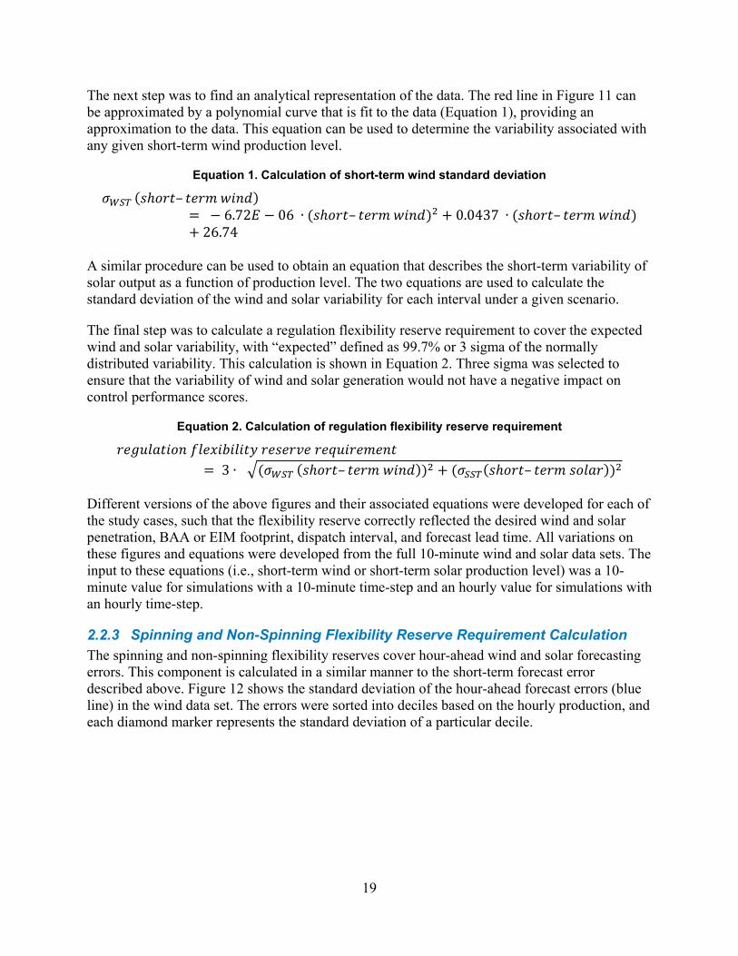
19
The next step was to find an analytical representation of the data. The red line in Figure 11 can be approximated by a polynomial curve that is fit to the data (Equation 1), providing an approximation to the data. This equation can be used to determine the variability associated with any given short-term wind production level.
Equation 1. Calculation of short-term wind standard deviation
𝜎𝑊𝑆𝑇 (𝑠ℎ𝑜𝑟𝑡– 𝑡𝑒𝑟𝑚 𝑤𝑖𝑛𝑑)= − 6.72𝐸 − 06 ∙ (𝑠ℎ𝑜𝑟𝑡– 𝑡𝑒𝑟𝑚 𝑤𝑖𝑛𝑑)2 + 0.0437 ∙ (𝑠ℎ𝑜𝑟𝑡– 𝑡𝑒𝑟𝑚 𝑤𝑖𝑛𝑑)+ 26.74
A similar procedure can be used to obtain an equation that describes the short-term variability of solar output as a function of production level. The two equations are used to calculate the standard deviation of the wind and solar variability for each interval under a given scenario.
The final step was to calculate a regulation flexibility reserve requirement to cover the expected wind and solar variability, with “expected” defined as 99.7% or 3 sigma of the normally distributed variability. This calculation is shown in Equation 2. Three sigma was selected to ensure that the variability of wind and solar generation would not have a negative impact on control performance scores.
Equation 2. Calculation of regulation flexibility reserve requirement
𝑟𝑒𝑔𝑢𝑙𝑎𝑡𝑖𝑜𝑛 𝑓𝑙𝑒𝑥𝑖𝑏𝑖𝑙𝑖𝑡𝑦 𝑟𝑒𝑠𝑒𝑟𝑣𝑒 𝑟𝑒𝑞𝑢𝑖𝑟𝑒𝑚𝑒𝑛𝑡= 3 ∙ �(𝜎𝑊𝑆𝑇 (𝑠ℎ𝑜𝑟𝑡– 𝑡𝑒𝑟𝑚 𝑤𝑖𝑛𝑑))2 + (𝜎𝑆𝑆𝑇(𝑠ℎ𝑜𝑟𝑡– 𝑡𝑒𝑟𝑚 𝑠𝑜𝑙𝑎𝑟))2
Different versions of the above figures and their associated equations were developed for each of the study cases, such that the flexibility reserve correctly reflected the desired wind and solar penetration, BAA or EIM footprint, dispatch interval, and forecast lead time. All variations on these figures and equations were developed from the full 10-minute wind and solar data sets. The input to these equations (i.e., short-term wind or short-term solar production level) was a 10-minute value for simulations with a 10-minute time-step and an hourly value for simulations with an hourly time-step.
2.2.3 Spinning and Non-Spinning Flexibility Reserve Requirement Calculation The spinning and non-spinning flexibility reserves cover hour-ahead wind and solar forecasting errors. This component is calculated in a similar manner to the short-term forecast error described above. Figure 12 shows the standard deviation of the hour-ahead forecast errors (blue line) in the wind data set. The errors were sorted into deciles based on the hourly production, and each diamond marker represents the standard deviation of a particular decile.

20
Figure 12. Hour-ahead forecast error standard deviation as a function of wind production level
The red line in Figure 12 is a curve fit polynomial (Equation 3) that approximates the data. This equation can be used to determine the standard deviation of the forecast error associated with a previous hour’s production (persistence forecast).
Equation 3. Sample calculation of hour-ahead wind standard deviation
𝜎𝐻𝐴𝑊𝑖𝑛𝑑(ℎ𝑜𝑢𝑟𝑙𝑦 𝑤𝑖𝑛𝑑)= − 2.985𝐸 − 05 ∙ (ℎ𝑜𝑢𝑟𝑙𝑦 𝑤𝑖𝑛𝑑)2 + 0.1895 ∙ (ℎ𝑜𝑢𝑟𝑙𝑦 𝑤𝑖𝑛𝑑) + 103.2
A similar procedure can be used to obtain an equation that describes the hour-ahead forecast error of solar output as a function of production level. The two equations were used to calculate the standard deviation of the wind and solar forecast error for each interval under a given study scenario. Each study scenario had its own set of equations based on the number of BAAs represented and the aggregate wind and solar in each BAA.
Both spinning and non-spinning flexibility reserves cover the probable wind and solar forecast error. Spinning reserves cover one standard deviation of the forecast errors, or approximately 68%. Non-spinning reserves cover two standard deviation of the forecast errors, or approximately 95%. Equation 4 shows the calculation for the spinning reserves, and Equation 5 shows the calculation for the non-spinning reserves.
Equation 4. Calculation of spinning flexibility reserve requirement
𝑠𝑝𝑖𝑛𝑛𝑖𝑛𝑔 𝑓𝑙𝑒𝑥𝑖𝑏𝑖𝑙𝑖𝑡𝑦 𝑟𝑒𝑠𝑒𝑟𝑣𝑒 𝑟𝑒𝑞𝑢𝑖𝑟𝑒𝑚𝑒𝑛𝑡 = � 𝜎𝐻𝐴𝑊𝑖𝑛𝑑(𝑝𝑟𝑒𝑣𝑖𝑜𝑢𝑠 ℎ𝑜𝑢𝑟 𝑤𝑖𝑛𝑑)2 + 𝜎𝐻𝐴𝑆𝑜𝑙𝑎𝑟(𝑝𝑟𝑒𝑣𝑖𝑜𝑢𝑠 ℎ𝑜𝑢𝑟 𝑠𝑜𝑙𝑎𝑟)2

21
Equation 5. Calculation of non-spinning flexibility reserve requirement
𝑛𝑜𝑛 -𝑠𝑝𝑖𝑛𝑛𝑖𝑛𝑔 𝑓𝑙𝑒𝑥𝑖𝑏𝑖𝑙𝑖𝑡𝑦 𝑟𝑒𝑠𝑒𝑟𝑣𝑒 𝑟𝑒𝑞𝑢𝑖𝑟𝑒𝑚𝑒𝑛𝑡 = 2 ∗ � 𝜎𝐻𝐴𝑊𝑖𝑛𝑑(𝑝𝑟𝑒𝑣𝑖𝑜𝑢𝑠 ℎ𝑜𝑢𝑟 𝑤𝑖𝑛𝑑)2 + 𝜎𝐻𝐴𝑆𝑜𝑙𝑎𝑟(𝑝𝑟𝑒𝑣𝑖𝑜𝑢𝑠 ℎ𝑜𝑢𝑟 𝑠𝑜𝑙𝑎𝑟)2
Three-sigma total coverage was selected to ensure that the uncertainty associated with variable generation will not negatively affect control performance scores. The 1 sigma-2 sigma split for spinning and non-spinning resources was determined through an analysis of variable generation ramping data and the timeframes in which those ramps occur.
2.2.4 Effect of Forecast and Dispatch Timing on Forecast Error and Reserve Requirements
The discussion in the previous sections assumes a particular timing for forecast and dispatch. The short-term error example assumed that the forecast would be made 10 minutes before the beginning of the dispatch interval, which would last 10 minutes before a new dispatch would take effect. The method developed can be used to evaluate other timing as well.
Figure 13 shows how a different set of timings can affect forecast errors. In this example, the forecast for the next hour-long dispatch period is taken 40 minutes before the beginning of that period. That forecast is assumed valid throughout the entire hour of the dispatch. The difference between the hourly forecast and the actual wind and solar profile is a variation on the short-term forecast error shown in Figure 10.
Figure 13. Effect of hourly dispatch and 40-minute forecast lead on forecast error
Using the forecast error determined from the hourly persistence forecast, the flexibility reserve requirements can be calculated using the reserves method described above. These requirements are much higher because the reserves must of sufficient magnitude to cover the variability seen in an hour instead of 10 minutes, as seen in the earlier example.

22
Figure 14 shows the impact of geographic size and dispatch frequency on flexibility reserve requirements. The left box shows the flexibility reserve need from the full-participation EIM at alternative dispatch and forecast time-steps. The middle box shows the reserve implication of three regional EIM implementations, and the right box shows BAU. The time-steps are shown in the legend by two numbers. The first number is the dispatch time-step, and the second number is the forecast lead time or notification. For example 30-10 is a 30-minute dispatch with 10-minute-ahead forecast and notification. This graph shows that large BAAs with fast economic dispatch have smaller flexibility reserve requirements than small BAAs with slow economic dispatch.
Figure 14. Effect of dispatch interval and aggregation size on reserve requirements
2.3 Modeling Limitations It is not possible to model the Western Interconnection exactly as it will operate in 2020—either with or without the EIM. Limitations on the modeling include:
• A lack of data on bilateral power purchase agreements in place today or that will be in place in 2020. Lack of contractual data between generators, transmission providers, and load-serving entities has a significant impact on the commitment and dispatch performed by the production simulation software. Without such data, the software develops a minimum production cost commitment and dispatch, subject only to generating unit operating limits, transmission path ratings, and other performance constraints. Even if these agreements were made available for this study, it is possible that the terms of the energy exchanges could change by 2020. Thus, even if current agreements were modeled precisely, there is uncertainty regarding their future form. Because power purchase information is not available, the generally accepted approach is to use hurdle rates to provide transactional friction and limit economic power flows. The WECC-E3 study developed hurdle rates for each pair of BAAs so that flows in the model were closely aligned with actual flows from 2006. Those hurdle rates were also used in this analysis.

23
• Uncertainty regarding the use of other new or proposed tools to better coordinate wide-area operations in the West. Some of these tools, such as the dynamic scheduling system and ITAP, are designed to be used on an as-needed basis and therefore cannot be systematically captured in a modeling framework. Further, no data regarding the extent to which ITAP will be used were available for this study. This study focuses on the potential benefits of the EIM and does not evaluate other means of operational coordination that may emerge before 2020.
• Uncertainty regarding the impact of Federal Energy Regulatory Commission Order 764. This order requires transmission operators to offer 15-minute (or faster) transmission scheduling. However, the ruling does not appear to require the use of 15-minute schedules, only that transmission operators offer 15-minute scheduling to generators—including wind and solar generation owners. Therefore, it is not possible to know which entities will use these faster schedules or the extent to which the schedules will be used. The specific dispatch interval assumptions for both the BAU and EIM cases evaluated in this study are described in Section 2.4.
• Uncertainty regarding the amount and location of variable generation such as wind and solar energy. These assumptions are key drivers of the study results, and although alternative wind-solar scenarios were not evaluated with PLEXOS, prior work on flexibility reserves has shown a significant impact of penetration on reserve requirements (King et al. 2012). This study adopted the assumptions from TEPPC PC0 and the WECC-E3 study, which were vetted by WECC’s public stakeholder process. The 8% wind and 3% solar penetrations for 2020 were included in these assumptions.
• Uncertain transmission additions. New transmission may alleviate existing transmission constraints or allow more access to remote but economic generation. In addition, EIM transactions would flow at the lowest level of transmission service and therefore be subject to curtailment. If transactional curtailment were to be significantly more (or less) than expected, this would reduce (or increase) the value of the EIM. TEPPC PC0 assumptions regarding future transmission were incorporated.
• Uncertain generation additions and retirements between now and 2020. Specifically, there is significant uncertainty regarding coal retirements—which may be stimulated by new Environmental Protection Agency rules regarding emissions. These retirements would alter the future nonvariable generation mix, its flexibility characteristics, and fuel costs and therefore impact study results. The TEPPC PC0 assumptions regarding future generation were incorporated.
• Potential changes in the way hydro generation will be operated (e.g., because of drought) in the future. Hydro modeling is described in Section 2.5.2.3. The PLEXOS hydro model results were somewhat closer to the WECC TEPPC results than were the WECC-E3 results.

24
• Software limitations. Currently, CAISO and AESO operate 5-minute economic dispatch with compensation from energy markets. The rest of the interconnection generally operates on hourly schedules. The current generation of production simulation models cannot model different dispatch intervals within a single simulation. Thus, it is not possible to simultaneously model the 5-minute market and hourly nonmarket areas of the Western Interconnection.
• Uncertainty about gas and coal prices. The EIM will result in more efficient dispatch, thus reducing generation on the margin of the dispatch curve. When fuel prices are unknown, the value of the new dispatch is not known with certainty. Two gas price scenarios were evaluated.
• Uncertainty regarding which BAAs and generators would participate in the EIM. Both full and reduced EIM participation were evaluated.
• Ten-minute resolution load, wind, and solar data. The EIM would operate at a 5-minute time-step, so the use of 10-minute data gives slightly conservative results. A longer dispatch interval means higher flex reserve requirements for the EIM scenario and, therefore, less of a difference between it and the BAU case.
• The fact that quick-start units, similar to other thermal units, are committed in the day-ahead unit commitment step of PLEXOS simulations. That commitment is maintained throughout the SCED step. This results in committed combustion turbines (CTs) operating at minimum generation during the real-time dispatch. An improved model of quick-start CTs would allow these units to start and stop during real time rather than maintaining the day-ahead commitment and enforcing minimum generation operation.
Each of these items will have an impact on the BAU simulation results, the EIM simulation results, and the benefit calculation of the EIM. One set of study assumptions and modeling approximations, as described in this section, was used in this study to represent the key elements of the BAU and EIM study scenarios. Other assumptions and approximations could be analyzed in future studies. Therefore, the results of this study must be interpreted in the proper context as one possible outcome and not as a definitive forecast.
2.4 Study Cases Study cases were developed to identify the potential benefits of an EIM under various system conditions and assumptions and to confirm the consistency of this study’s results with those of the E3 study. For clarity, the cases are grouped in the following sections according to their purpose. Thus, the E3 alignment cases are described in Section 2.4.1, and the EIM benefit cases are described in Section 2.4.2.
To facilitate the following discussion, a naming convention for the simulation cases was developed. To minimize confusion, both the overall description of the case in question and the case name is used in the discussion. For example, E3BAU is a BAU case that aligns with the WECC-E3 study and uses an hourly time-step in the production simulations, whereas PLHBAU is a new PLEXOS BAU case that uses an hourly time-step.

25
Table 3. Case-Naming Convention
Part 1 Part 2 and/or 3 E3 Aligns with the WECC-E3 study,
hourly time-step BAU Business as usual
PL PLEXOS case, 10-minute time-step
EIM1 EIM using PLHBAU day-head commitment
PLH PLEXOS case, hourly time-step EIM2 EIM using E3BAU day-ahead commitment PMA1 Federal power marketing administrations excluded
from EIM, using PLHBAU day-head commitment PMA2 Similar to PMA1 but with E3BAU day-head
commitment RES Reduced reserve GAS Lower gas price
2.4.1 E3 Alignment Cases Two cases were developed to check the alignment of the results of this study, which used 10-minute simulations and PLEXOS software, with those of the E3 study, which used 1-hour simulations and GridView software. Regardless of the simulation time-step, the alignment cases are referred to as 10-minute cases because the flexibility reserves were calculated assuming a 10-minute dispatch interval and a 10-minute forecast lead time.
The first case, E3BAU is an hourly simulation with few changes to Western Interconnection operating procedures between now and 2020. Thus, it is termed a BAU case and acts as a benchmark for comparison with the case of the full EIM footprint. This case includes:
• Hourly simulation time-step • Hourly dispatch of generation • 10-minute lockdown or lead time for forecasts • 10-minute flex reserve requirements.
In this case:
• Individual BAs perform their own unit commitment to meet their own load and reserve requirements with their own generation
• Individual BAs perform their own dispatch to balance load and generation
• All BAA hurdle rates are implemented.
The forecast lead time, also referred to as the forecast lockdown time, is the time period between when the forecast for the load and variable generation is fixed for a given dispatch interval and the beginning of that dispatch interval. In this study, the forecast for variable generation is taken as a persistence forecast. That is, the value of wind or solar generation is assumed to be constant over the dispatch interval as measured at the forecast lead time.

26
The hourly unit commitment is developed from the hourly wind forecast, hourly actual solar, and hourly actual load. Thus, the solar and load forecasts used are perfect. Each BA commits its units to meet its forecasted net load (actual load minus forecasted wind minus actual solar) and reserve requirements. The economic dispatch step uses hourly actual wind, solar, and load data. It results in a chronological hourly dispatch and interchange results for the study year. Each BA dispatches its units to meet its actual net load (actual load minus actual wind minus actual solar) and reserve requirements.
Reserve requirements include the standard contingency reserve and the new flexibility reserve necessary to accommodate the variability and uncertainty of wind and solar power. These flex reserve requirements are calculated using the hourly wind or solar production level as an input to a case-specific set of equations based on the 10-minute data, as described in the previous section. As noted above, the flexibility reserve calculations must be performed for each region or aggregation of regions studied. For this BAU case, each BA within the study footprint is responsible for managing the variability within its boundaries. These calculations are performed on the data specific to each BAA, such as the aggregate wind and solar production profiles. These profiles are aggregated from individually modeled plants and thus fully represent the geographic and temporal diversity of their BAA. The result of this analysis is 8760 hours of combined flex regulation and flex spin for each BA, which are used in the production simulation analysis.
The second alignment case, E3EIM, represents the operation of the EIM with full participation. The full EIM footprint consists of the Western Interconnection without the areas that already have markets in place (CAISO and AESO). A comparison of this case with the benchmark, E3BAU, will show the potential EIM benefits under study assumptions similar to those of the E3 study. This case includes:
• Hourly simulation time-step • Hourly dispatch of generation • 10-minute lockdown or lead time for forecasts • 10-minute flex reserve requirements.
In this case:
• Individual BAs perform their own unit commitment to meet their own load and reserve requirements with their own generation
• Dispatch of imbalance is performed across the full EIM footprint to balance load and generation
• The hurdle rates between the BAAs within the EIM footprint are removed. Hurdle rates remain between the EIM participants (e.g., SRP) and nonparticipants (e.g., CAISO).
The flex reserve requirements are calculated using the hourly wind or solar production level as an input to a set of equations specific to the 10-minute data for the entire EIM footprint.

27
2.4.2 EIM Benefit Cases The majority of cases were developed to explore the potential benefits of an EIM. Given the inherent difficulty of predicting the future, the primary objective in designing these cases was to cover a range of possible scenarios.
One series of cases uses the E3BAU case, described in the previous subsection, as a benchmark. The three other cases in this series represent system operation with full EIM participation, reduced EIM participation, and reduced flexibility reserves. Regardless of the simulation time-step, these cases are referred to as 10-minute cases because the flexibility reserves are calculated assuming a 10-minute dispatch interval and a 10-minute forecast lead time.
The PLEIM2 case examines the operation with full EIM participation, which means the Western Interconnection without the areas that already have markets (i.e., CAISO and AESO). A comparison of this case with the benchmark, E3BAU, will show the potential benefit of the full EIM footprint for one set of assumptions. It includes:
• 10-minute simulation time-step • 10-minute dispatch of generation • 10-minute lockdown or lead time for forecasts • 10-minute flex reserve requirements.
In this case:
• The same unit commitment as E3BAU is used
• Dispatch is performed across the full EIM footprint to balance load and generation
• The hurdle rates between the BAAs within the EIM footprint are removed. Hurdle rates remain between the EIM participants and nonparticipants.
For this and other EIM cases, the wind and solar production profiles for each BAA are further aggregated into profiles for a given EIM footprint. Again, the geographic and temporal diversity of the data are preserved. A different set of combined flex regulation and flex spin reserves will result for this case. Aggregating the variable generation reduces the overall variability of the combined regions. This leads to lower aggregate reserve requirements.
The PLEIM-PMA2 case was designed to explore the sensitivity of the potential EIM benefits to reduced participation in the EIM. The full EIM included participation of the entire Western Interconnection except those areas that already have markets. Requested by the Public Utility Commission Energy Imbalance Market (PUC EIM) Group, this reduced footprint excludes BPA and two of the three Western Area Power Administration (WAPA) BAs. Several entities (CHPUD, DOPUD, GCPUD, Seattle City Light, and Tacoma Power) embedded in BPA are also excluded. This case includes:
• 10-minute simulation time-step • 10-minute dispatch of generation • 10-minute lockdown or lead time for forecasts • 10-minute flex reserve requirements.

28
In this case:
• The same unit commitment as E3BAU is used
• Dispatch is performed across the reduced EIM footprint to balance load and generation
• The hurdle rates between the BAAs within the EIM footprint are removed. Hurdle rates remain between the EIM participants and nonparticipants.
The final case in this series, PLRES, carries reduced flexibility reserves across the full EIM footprint. Only the regulation component of the flexibility reserves is used. (This assumes flex spin can be released in real time.) This case, developed at the suggestion of industry stakeholders, provides information about the sensitivity of results to the potential release of non-spin, which contrasts with other cases. This case includes:
• 10-minute simulation time-step • 10-minute dispatch of generation • 10-minute lockdown or lead time for forecasts • 10-minute flex reserve requirements for regulation only.
In this case:
• The same unit commitment as E3BAU is used
• Dispatch is performed across the full EIM footprint to balance load and generation
• The hurdle rates between the BAAs within the EIM footprint are removed. Hurdle rates remain between the EIM participants and nonparticipants.
A second series of cases begins with a different benchmark case: PLHBAU. PLHBAU is an hourly simulation with few changes to Western Interconnection operating procedures between now and 2020. It is referred to as an hourly case because the flexibility reserves are calculated assuming an hourly dispatch interval and a 40-minute forecast lead time. This hourly BAU case and the 10-minute BAU case (E3BAU, described above) act as bookends to the range of possible scenarios. This case includes:
• Hourly simulation time-step • Hourly dispatch of generation • 40-minute lockdown or lead time for forecasts • Hourly flex reserve requirements.
In this case:
• Individual BAs perform their own unit commitment to meet their own load and reserve requirements with their own generation
• Individual BAs perform their own dispatch to balance load and generation
• All BAA hurdle rates are implemented.

29
The forecast lead time, also referred to as the forecast lockdown time, is the time period between when the forecast for load and variable generation is fixed for a given dispatch interval and the beginning of that dispatch interval. In this study, the forecast for variable generation is taken as a persistence forecast. That is, the value of wind or solar generation is assumed to be constant over the dispatch interval as measured at the forecast lead time. For this hourly BAU case, the forecast lockdown was 40 minutes. Therefore, this forecast will be 1 hour and 40 minutes out of date by the end of the dispatch interval.
The hourly unit commitment is developed from the hourly wind forecast, hourly actual solar, and hourly actual load. Thus, the solar and load forecasts used are perfect. Each BA commits its units to meet its forecasted net load (actual load minus forecasted wind minus actual solar) and reserve requirements. The economic dispatch step uses hourly actual wind, solar, and load data. It results in a chronological hourly dispatch and interchange results for the study year. Each BA dispatches its units to meet its actual net load (actual load minus actual wind minus actual solar) and reserve requirements.
Reserve requirements include the standard contingency reserve and the new flexibility reserve necessary to accommodate the variability and uncertainty of wind and solar. These flex reserve requirements are calculated using the hourly wind or solar production level as an input to a case-specific set of equations, as described in the previous section. As noted above, the flexibility reserve calculations must be performed for each region or aggregation of regions studied. For this BAU case, each BA within the study footprint is responsible for managing the variability within its boundaries. These calculations are performed on the 10-minute data specific to each BAA, such as the aggregate wind and solar production profiles as well as the forecast lead time. These profiles are aggregated from individually modeled plants and thus fully represent the geographic and temporal diversity of their BAA. The result of this analysis is 8760 hours of combined flex regulation and flex spin for each BA. This is used in the production simulation analysis.
Two EIM cases are included in this series. PLEIM1 examines operation with full EIM participation. It is similar to PLEIM2 in its assumptions but starts with a different unit commitment. It includes:
• 10-minute simulation time-step • 10-minute dispatch of generation • 10-minute lockdown or lead time for forecasts • 10-minute flex reserve requirements.
In this case:
• The same unit commitment as PLHBAU is used
• Dispatch is performed across the full EIM footprint to balance load and generation
• The hurdle rates between the BAAs within the EIM footprint are removed. Hurdle rates remain between the EIM participants and nonparticipants.

30
The PLEIM-PMA1 case was designed to explore the sensitivity of the potential EIM benefits to reduced participation in the EIM. This reduced footprint excludes BPA, its embedded utilities (CHPUD, DOPUD, GCPUD, SCL, and TPWR), and two of the three WAPA BAs. It is similar to the PLEIM-PMA2 case in its assumptions but starts with a different unit commitment. This case includes:
• 10-minute simulation time-step • 10-minute dispatch of generation • 10-minute lockdown or lead time for forecasts • 10-minute flex reserve requirements.
In this case:
• The same unit commitment as PLHBAU is used
• Dispatch is performed across the reduced EIM footprint to balance load and generation
• The hurdle rates between the BAAs within the EIM footprint are removed. Hurdle rates remain between the EIM participants and nonparticipants.
A final pair of sensitivity cases was designed to evaluate the impact of reduced natural gas prices on potential EIM benefits. The WECC TEPPC 2020 planning case that is the basis of this analysis uses a gas price of $7.28/MMBtu. A lower price of $4.50/MMBtu (Henry Hub benchmark) was used for the final cases. This lower gas price is consistent with the newer TEPPC 2022 cases, which included a natural gas price of $4.60/MMBtu. The first case, PLGASBAU, is similar to the PLHBAU case but with a lower gas price. This case includes:
• Hourly simulation time-step • Hourly dispatch of generation • 40-minute lockdown or lead time for forecasts • Hourly flex reserve requirements.
In this case:
• Individual BAs perform their own unit commitment to meet their own load and reserve requirements with their own generation
• Individual BAs perform their own dispatch to balance load and generation
• All BAA hurdle rates are implemented.
The second case, PLGASEIM, examines operation with full EIM participation. A comparison of this case to the benchmark, PLGASBAU, will show the potential benefit of full EIM participation at the lower gas price. This case includes:
• 10-minute simulation time-step • 10-minute dispatch of generation • 10-minute lockdown or lead time for forecasts • 10-minute flex reserve requirements.
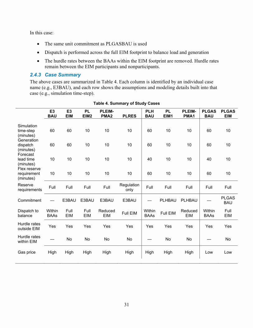
31
In this case:
• The same unit commitment as PLGASBAU is used
• Dispatch is performed across the full EIM footprint to balance load and generation
• The hurdle rates between the BAAs within the EIM footprint are removed. Hurdle rates remain between the EIM participants and nonparticipants.
2.4.3 Case Summary The above cases are summarized in Table 4. Each column is identified by an individual case name (e.g., E3BAU), and each row shows the assumptions and modeling details built into that case (e.g., simulation time-step).
Table 4. Summary of Study Cases
E3 BAU
E3 EIM
PL EIM2
PLEIM-PMA2 PLRES
PLH BAU
PL EIM1
PLEIM-PMA1
PLGAS BAU
PLGAS EIM
Simulation time-step (minutes)
60 60 10 10 10 60 10 10 60 10
Generation dispatch (minutes)
60 60 10 10 10 60 10 10 60 10
Forecast lead time (minutes)
10 10 10 10 10 40 10 10 40 10
Flex reserve requirement (minutes)
10 10 10 10 10 60 10 10 60 10
Reserve requirements Full Full Full Full Regulation
only Full Full Full Full Full
Commitment — E3BAU E3BAU E3BAU E3BAU — PLHBAU PLHBAU — PLGAS BAU
Dispatch to balance
Within BAAs
Full EIM
Full EIM
Reduced EIM Full EIM Within
BAAs Full EIM Reduced EIM
Within BAAs
Full EIM
Hurdle rates outside EIM Yes Yes Yes Yes Yes Yes Yes Yes Yes Yes
Hurdle rates within EIM — No No No No — No No — No
Gas price High High High High High High High High Low Low

32
2.5 Production Simulation Model A production cost model simulates the operation of the interconnected generation and transmission system by solving at each time interval the least-cost solution to generating sufficient energy to meet demand. The solution is influenced by transmission constraints [direct current (DC) optimal power flow (DCOPF) on the nodal system representation], generator operation properties (e.g., start-up costs, ramp rates, and maintenance outages), and reserve requirements for meeting intra-interval generation-demand imbalances. Operators run production cost models for planning purposes (e.g., to test capacity expansion feasibility) and during daily/hourly operation to schedule generating units.
For this study, a commercial production simulation tool, PLEXOS, was used. The production simulations were performed by the software developer, Energy Exemplar Ltd. PLEXOS has hourly and subhourly simulation capability. Both were used in this study. Hourly simulations were used to emulate current operating practices in the Western Interconnection, and subhourly simulations were used to capture the impact of subhourly operations as well as the subhourly variability and uncertainty of wind and solar.
A multistage simulation process was used to emulate power system operation. The first stage developed an initial profile for hydro generation based on monthly energy production while respecting minimum and maximum capacity. The second stage mimicked the hourly day-ahead SCUC, and the third stage mimicked the real-time SCED using the unit commitment schedules and hydro profiles from the prior stages. The time interval for the first and third stages was either hourly or 10 minutes, depending on the study scenario. The second stage or unit commitment used a 1-hour time interval.
2.5.1 PLEXOS Software Overview PLEXOS has three levels of simulation: a long-term plan for capacity expansion simulations; a medium-term schedule for optimizing hydro storage, fuel supplies, or emissions; and a short-term schedule for chronological unit commitment and dispatch. The latter two capabilities were used in this study.
The medium-term schedule was used to develop hourly (or 10-minute) hydro profiles based on monthly energy requirements and unit minima and maxima. This logic performs the co-optimization of energy and ancillary services for an entire month at the regional level. The hours in a month are grouped into 90 time blocks in the descending order of a load duration curve, with each time block an interval in the optimization. The outputs of this step are hydro generation profiles that honor the monthly hydro energy constraints. Chronological hydro unit constraints, such as ramp rate limitations, are not enforced in this part of the process.

33
The short-term schedule was used once for the SCUC to emulate the day-ahead commitment process and a second time for the SCED to emulate real-time operation. The SCUC-SCED simulation algorithm is illustrated in Figure 15.
Figure 15. PLEXOS security-constrained unit commitment and economic dispatch algorithm
The unit commitment-economic dispatch logic performs the energy-ancillary services co-optimization by mixed integer programming, while enforcing all resource and operation constraints. The unit commitment-economic dispatch algorithm commits and dispatches resources to balance system energy demand and meet system reserve requirements. The hydro generation profiles developed in the first step are input to this step in the simulation process. The hydro schedules may be modified in this second step to respect chronological hydro unit constraints (e.g., ramp rates) or to respond to price signals.
The resource schedules from the unit commitment-economic dispatch logic are passed to the network application logic. The network application logic solves the DCOPF to enforce the power flow limits (i.e., transmission line or interface limits) and nomograms (i.e., limits based on a specific relationship between generation, load, transmission topology, and/or interface power flows). The network application logic also performs a contingency analysis for defined contingencies, although none were defined for this study. If there are transmission limit violations, the limits are passed to the unit commitment-economic dispatch logic for a re-run. The iteration continues until all transmission limit violations are resolved. Thus, the co-optimized solution of energy-ancillary services-DCOPF is reached.
DC - OPF solves network power flow for the resource schedules passed from unit
Perform s contingency power flow analysis Enforce s transmission line limits , interface limits , and nomograms
Energy - a n c i l l a r y s e r v i c e co - optimization by mixed integer programming Enforce s resource chronological constraints, transmission constraints passed from network applications, and other constraints Solutions include resource on - line status, loading levels, and a n c i l l a r y s e r v i c e provisions
Unit Commitment- Economic Dispatch
Resource Schedule
Violated Transmission Constraints
Network Applications
commitment-economic dispatch

34
Shortages of generating capacity, over-supply of energy, and transmission congestion are recognized and measured in terms of unserved energy, spilled energy, and reserve shortfall. When this occurs, the energy balance constraint or reserve requirement constraint is relaxed. The order of the relaxation of these constraints is determined by the slack penalty prices of the constraints. The constraints with a smaller slack penalty price are relaxed first. As shown in Table 5, the order of relaxation is: (1) spill energy, (2) contingency spinning reserve shortfall, (3) flexibility reserve shortfall, and (4) unserved energy.
Table 5. Order of Constraint Relaxation
Constraints Slack Variables Penalty Price Energy balance
Spill energy -$20/MWh
Contingency reserve
Spin shortfall $250/MWh
Flexibility reserve
Flexibility shortfall $400/MWh
Energy balance Unserved energy $500/MWh
In this study, the wind and solar generation were treated as noncurtailable.
The day-ahead SCUC optimizes over 24 hours, with an hourly interval. Input data include:
• Forecasted wind generation profiles
• Actual load and solar generation profiles (i.e., perfect forecasts)
• Detailed generator characteristics
• Contingency reserve, regulation reserve, and flexibility reserve for each specified BAA or group of BAAs
• Transmission hurdle rates between BAAs
• Detailed nodal transmission network of the Western Interconnection.
The day-ahead SCUC simulation results in an hourly unit commitment and resource schedule for the entire interconnection. Each BA commits enough online capacity to cover its own load and reserve requirements at any hour.
For hourly cases, the real-time SCED optimizes over the hour with no look-ahead. For 10-minute cases, the real-time SCED optimizes over 10 minutes with a look-ahead of five 10-minute intervals. Input data for either include:
35
• The actual load, wind, and solar profiles
• Unit commitment schedules from the day-ahead SCUC
• Detailed generator characteristics
• Contingency reserve, regulation reserve, and flexibility reserve for each specified BAA or group of BAAs
• Transmission hurdle rates between BAAs
• The detailed nodal transmission network of the Western Interconnection.
The real-time SCED simulation results in either an hourly or 10-minute dispatch for the interconnection.
The flexibility reserves to cover the renewable variability and uncertainty are included in both the day-ahead SCUC and the real-time SCED. For the day-ahead simulations, the flexibility reserves are defined at the BAA level. For the 10-minute real-time simulations, the flexibility reserves are defined at the BAA level for the BAU scenario and at the EIM footprint level for EIM scenarios.
2.5.2 System Model The WECC TEPPC 2020 PC0 system model was used in this study. It was converted directly from the TEPCC PROMOD format to PLEXOS format. This model includes the transmission and generation systems as well as the regional definitions used for contingency reserves. Each is described in more detail below. The PLEXOS version of this model is essentially the same as the original TEPPC model. In addition, study assumptions were drawn from the E3 study to enable comparisons of results. Modifications made for the purposes of this study are reported below.
2.5.2.1 Transmission System Model The transmission network model represents the entire Western Interconnection and includes:
• More than 17,500 nodes • More than 22,590 transmission lines and transformers • 1043 transmission lines and transformer limits that are enforced • 44 phase shifters modeled as control variables • More than 120 interfaces whose limits are enforced • 8 nomograms, including several multisegment ones • 39 regions.
The interfaces that were enforced and their limits are shown in the appendix. The nomograms are shown in Table 6.
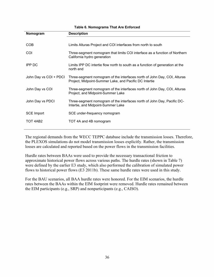
36
Table 6. Nomograms That Are Enforced
Nomogram Description
COB Limits Alturas Project and COI interfaces from north to south
COI Three-segment nomogram that limits COI interface as a function of Northern California hydro generation
IPP DC Limits IPP DC intertie flow north to south as a function of generation at the north end
John Day vs COI + PDCI Three-segment nomogram of the interfaces north of John Day, COI, Alturas Project, Midpoint-Summer Lake, and Pacific DC Intertie
John Day vs COI Three-segment nomogram of the interfaces north of John Day, COI, Alturas Project, and Midpoint-Summer Lake
John Day vs PDCI Three-segment nomogram of the interfaces north of John Day, Pacific DC-Intertie, and Midpoint-Summer Lake
SCE Import SCE under-frequency nomogram
TOT 4AB2 TOT 4A and 4B nomogram
The regional demands from the WECC TEPPC database include the transmission losses. Therefore, the PLEXOS simulations do not model transmission losses explicitly. Rather, the transmission losses are calculated and reported based on the power flows in the transmission facilities.
Hurdle rates between BAAs were used to provide the necessary transactional friction to approximate historical power flows across various paths. The hurdle rates (shown in Table 7) were defined by the earlier E3 study, which also performed the calibration of simulated power flows to historical power flows (E3 2011b). These same hurdle rates were used in this study.
For the BAU scenarios, all BAA hurdle rates were honored. For the EIM scenarios, the hurdle rates between the BAAs within the EIM footprint were removed. Hurdle rates remained between the EIM participants (e.g., SRP) and nonparticipants (e.g., CAISO).

37
Table 7. Hurdle Rates Between BAAs
There are many transmission rights in the Western Interconnection. Only those transmission rights with complete information were modeled. The transmission reconfiguration used to model these transmission rights is described below. These changes were necessary to allow the unit commitment to be performed accurately in the affected areas.
From BAA To BAA $/MWh
From BAA To BAA $/MWh
Forward Backward Forward Backward Alberta British Columbia 4.72 3.63 New Mexico EPE 5.43 5.63 Alberta NWE 4.72 3.63 New Mexico WALC 5.43 3.64 AVA British Columbia 4.07 3.63 NNV California 6.04 3.88 AVA BPA 4.07 3.26 NNV LADWP 40 9.68 AVA PACW 4.07 5.06 NNV NVP 6.04 3.03 AVA PGN 4.07 1.62 NWE AVA 14.72 4.07 AZPS California 9.62 3.88 NWE BPA 14.72 3.26 AZPS IID 2.12 4.13 NWE PACE 14.72 5.06 AZPS LADWP 9.62 9.68 NWE WACM 12.22 7.27 AZPS New Mexico 2.12 5.43 PACE AZPS 12.56 3.62 AZPS SRP 2.12 2.98 PACE California 40 9.68 AZPS TEP 2.12 4.88 PACE IPC 5.06 3.86 AZPS WALC 2.12 3.64 PACE LADWP 40 9.68 BPA BANC 8.94 5.99 PACE NVP 12.56 2.03 BPA British Columbia 3.26 3.63 PACE NNV 5.06 6.04 BPA California 11.44 7.29 PACE WACM 10.06 7.27 BPA LADWP 8.94 9.68 PACE WALC 12.56 2.64 BPA NNV 6.44 6.04 PACW California 10.06 3.88 BPA PACW 3.26 5.06 PACW PGN 5.06 1.62
BPA PGN 3.26 1.62
PSCO New Mexico 9.22 5.43
BPA PSE 3.26 0.96 PSCO WALC 11.72 3.64 California BANC 3.88 5.99 SRP California 7.98 3.88 EPE California 20.13 10.88 SRP TEP 2.98 4.88 IID California 4.13 3.88 SRP WALC 2.98 3.64 IPC AVA 11.36 4.07 TEP EPE 4.88 5.63 IPC BPA 11.36 3.26 TEP New Mexico 2.38 5.43 IPC NNV 11.36 6.04 WACM New Mexico 14.77 5.43 IPC PACW 11.36 5.06 WACM PSCO 14.77 4.22 IPC PGN 11.36 1.62 WACM WALC 14.77 3.64 LADWP California 9.68 3.88 WALC California 8.64 3.88 NVP California 8.03 3.88 WALC IID 3.64 4.13 NVP LADWP 8.03 9.68 WALC LADWP 8.64 9.68 NVP WALC 3.03 3.64 WALC TEP 3.64 4.88

38
2.5.2.2 Modifications to the Transmission Network SMUD has transmission rights to the California-Oregon Transmission Project. To capture that in the simulations, the California-Oregon Transmission Project from Captain Jack (BPA Bus 45035) to Olinda (PG&E Bus 30020) was reconfigured to terminate at an adjacent SMUD bus (Olinda West 37565). This line is subject to the hurdle rates between BPA and SMUD in the BAU and reduced-EIM participation cases but is not subject to the hurdle rate in the full-EIM participation case.
CAISO has transmission rights to the Pacific Northwest DC tie. To capture that in the simulations, one of the two DC lines from Celilo (BPA) to Sylmar (LADWP) was reconfigured to terminate at Sylmar (Bus 24147). Because this is an SCE bus and SCE is part of CAISO, this method represents CAISO’s transmission rights. Each DC line has a rated capacity of 1550 MW. The BPA-LADWP DC line is subject to the hurdle rate between BPA and LADWP in the BAU and the reduced-EIM participation cases but is not subject to the hurdle rate in the full-EIM participation case. The BPA-SCE DC line is subject to the hurdle rate between BPA and CAISO in all cases.
CAISO also has transmission rights to the Intermountain DC tie. The DC line from Intermountain (Bus 26114 LADWP) to Adelanto (Bus 26003 LADWP) was split into two DC lines. One DC line, with a capacity of 2064 MW, still terminates at the LADWP Adelanto bus. The second DC line, with a capacity 1526 MW, terminates at Lugo, which is an SCE bus (24086). The Intermountain-LADWP DC line is not subject to the hurdle rate in any case. The Intermountain-SCE DC line is subject to the hurdle rate between LADWP and CAISO in all cases.
IID has transmission rights to the Southwest Power Link. To capture this in the simulations, a fictitious DC line was created with the capacity of 195 MW from SRP (Bus 15090) to IID (Bus 21025). The fictitious line is in the interface AZPS-IID, which was subject to the SRP-IID hurdle rate in the BAU case and is not subject to this hurdle rate in the EIM cases.
2.5.2.3 Generation System Model There are also more than 2200 generators representing the Western Interconnection in the database. All generator characteristics were modeled in the PLEXOS simulations: minimum and maximum capacity, minimum up and down times, maximum ramp rates up and down, startup costs, etc.
The variable renewable resources (i.e., wind and solar) were modeled with either the forecasted or actual generation profiles, as appropriate for either the unit commitment or economic dispatch modules.
All thermal generators were modeled with heat rate and designated fuels with specified fuel prices and variable operating and maintenance charges. All heat rate and ramp rate data were generic, rather than unit-specific, as supplied by WECC TEPPC PC0.
The combined-cycle (CC) plants were modeled at the plant level, consistent with the original WECC TEPPC database. This means a single generator with appropriate data represented the combination of steam and CT generators that make up a CC plant.

39
In the PLEXOS database, the Henry Hub gas price of $7.28/MMBTU (2009 dollars) was used to derive the regional gas prices on a monthly basis in the same manner as in the E3 study. For the lower gas price sensitivity scenario, $4.50/MMBTU (2009 dollars) at Henry Hub was used to derive the regional gas prices. The regional coal prices are shown in Table 8. No carbon tax was used.
Table 8. Regional Coal Prices
Region $/MMBTU AESO 1.49 APS 1.88 BPA 2.12 FAR EAST 1.49 LDWP 1.21 NEVP 1.73 NWMT 1.04 PACE_UT 1.21 PACE_WY 0.98 PG&E_BAY 1.73 PG&E_VLY 1.73 PGN 2.12 PNM 1.38 PSC 1.42 SCE 1.73 SPPC 1.73 SRP 1.88 TEP 1.88 WACM 1.42 WALC 1.88
Two types of hydro models were used in the production simulation. The first represents a hydro plant’s annual production as a fixed generation profile. The second represents a more dispatchable hydro plant with a PLEXOS model that approximates the hydro-thermal coordination approach used to dispatch hydro in the Western Interconnection. The amount of hydro energy represented as fixed hourly generation profiles and the amount dispatched by PLEXOS is shown in Table 10.
Table 9. Hydro Energy Represented by Each Type of Model
Fixed Profile Dispatchable GWhr 58,696 188,169 % 24% 76%
The fixed hydro generation profiles were included in the TEPPC model and directly converted into PLEXOS.

40
The dispatchable hydro schedules were developed in a multistage process. First, the medium-term schedule was used to develop hourly (or 10-minute) hydro profiles based on monthly energy requirements and unit minima and maxima. This logic performs the co-optimization of energy and ancillary services for an entire month at the regional level. The hours in a month are grouped into 90 time blocks in the descending order of a load duration curve, with each time block an interval in the optimization. The output of this step is hydro generation profiles that honor the monthly hydro energy constraints. Chronological hydro unit constraints, such as ramp rate limitations, are not enforced in this part of the process. Second, the short-term schedule was used for the SCUC-SCED to commit and dispatch resources to balance the system energy demand and meet the system reserve requirements. The hydro generation profiles developed in the first step are input to this step in the simulation process. The hydro schedules may be modified in this second step to respect chronological hydro unit constraints (e.g., ramp rates), respond to price signals, or respect any transmission limits. The dispatchable hydro model was tuned to better match prior TEPPC simulation results, as shown in Figure 16.
Figure 16. Hydro dispatch comparison between this study and TEPPC results
To calculate the societal benefit of the EIM, detailed information regarding plant ownership and power purchase agreements are not critical inputs. However, because this study calculates the benefit of the EIM to each BAA, more specific data are required. There are many jointly owned generation resources in the Western Interconnection. When a generation resource is outside the owner’s BAA, additional modeling detail is required to ensure that the simulated commitment and dispatch of that unit is realistic. Complete ownership information was provided for only four generating plants: BPA, Hoover, Colstrip, and Mid-Columbia. The joint-ownership models for those plants are described below.
Because the owners of the BPA hydro power plants are already within the BPA BAA, there was no need to model the ownership explicitly to achieve a realistic commitment and dispatch.

41
The owners of the Hoover hydro power plant are listed in Table 10. The ownership is officially defined as a percentage of the entire power plant capacity and energy. The assignment of individual unit ownership is for the convenience of the modeling.
Because the Hoover plant is connected radially to the rest of the system, it was decided that each unit could be connected to the nearest bus of the owner through a fictitious DC line with minimal impact to surrounding power flows. The unit capacity is included in the owner’s commitment and reserve requirement constraints, and the power flows from Hoover hydro plant to the owners are not subject to the BAA hurdle rates.
Table 10. Hoover Hydro Power Plant Joint Ownership
Region Hoover Unit % Ownership WALC HOOVERA3_1 6% APS HOOVERA4_1 6% SRP HOOVERA5_1, HOVRA8A9_A8 9% NEVP HOOVERA6_1, HOOVERA7_1, HOVRA1A2_A1, HOVRA1A2_A2 25% LADWP HOVRA8A9_A9, HOVRN1N2_N1, HOVRN1N2_N2, 16% CAISO HOVRN3N4_N3, HOVRN3N4_N4, HOVRN5N6_N5, HOVRN5N6_N6,
HOVRN7N8_N7, HOVRN7N8_N8 37% The owners of the Colstrip Thermal Power Plant are listed in Table 11. For this plant, the ownership is defined as a percentage of individual units. Because of the interconnected transmission network around the Colstrip plant, no fictitious DC lines were used to connect these units to their owner’s system. The potential impact of such fictitious lines on parallel power flows was deemed too high. The unit capacity is included in the owner’s commitment and reserve requirement constraints. However, the power flows from Colstrip to the owners are subject to any BAA hurdle rates.
Table 11. Colstrip Thermal Power Plant Joint Ownership
Owner % Ownership Units NWMT 50 Colstrip #1 and #2 PSE 50 AVA 15
Colstrip #3 and #4 NWMT 30 PACE 10 PGN 20 PSE 25
Information about the joint ownership of the Mid-Columbia hydro power plants was also provided. The majority (50%–75%) of the owners of those units—BPA, SCL, TPWR, CHPD, DOPD, and GCPD—are within the BPA BAA. The remainder (25%–50%)—AVA, PACW, PGN, and PSE—are outside the BPA BAA. No fictitious DC lines were used to connect these

42
hydro units to the minority owners. Therefore, the unit capacity is included in the owner’s commitment and reserve requirement constraints. The power flow from Mid-Columbia to the majority owners is not subject to BAA hurdle rates. However, the power flow to the minority owners is subject to any BAA hurdle rates.
2.5.2.4 Regional Definitions For this study, 24 individual BAAs were represented across the Western Interconnection, as shown in Table 12 (repeated from Table 1). Several are aggregations of the 39 original load regions in the database. For example, the BPA area includes five embedded utilities—Chelan County Public Utility District, Douglas County Public Utility District, Grant County Public Utility District, Seattle City Light, and Tacoma Power—and is treated as a single large entity. BAAs that did not contain load were consolidated with the nearest BAA with load.
Table 12. BAAs Defined for This Study
BAAs BAAs Alberta Electric System Operator (AESO) Imperial Irrigation District (IID) Arizona Public Service (AZPS) Los Angeles Department of Water and Power (LADWP) Avista (AVA) Nevada Power (NEVP) Balancing Area of Northern California (BANC) Northern Nevada [Sierra Pacific Power Co. (SPPC)]
Sacramento Municipal Utility District (SMUD) Northwest Energy (NWE) Turlock Irrigation District (TID) Northwest Montana (NWMT)
Bonneville Power Administration (BPA) Western Area Upper Missouri (WAUM) PUD No. 1 of Chelan County (CHPD) Pacificorp East (PACE) PUD No. 1 of Douglas County (DOPD) Pacificorp Idaho (PACE_ID) PUD No. 1 of Grant County (GCPD) Pacificorp Utah (PACE_UT) Seattle City Light (SCL) Pacificorp Wyoming (PACE_WY) Tacoma Power (TPWR) Pacificorp West (PACW)
British Columbia Transmission Corp. (BCTC) or BC Hydro
Portland General Electric (PGN)
California Independent System Operator (CAISO) Public Service Company of Colorado (PSCO) Pacific Gas and Electric (PG&E) Public Service Company of New Mexico (PNM) Southern California Edison (SCE) Puget Sound Energy (PSE) San Diego Gas and Electric (SDGE) Salt River Project (SRP) Comision Federal de Electricidad (CFE) Tucson Electric Power (TEP)
El Paso Electric (EPE) Western Area Colorado Missouri (WACM) Idaho Power Corp. (IPC) Western Area Lower Colorado (WALC)
Far East (FAR EAST) Magic Valley (MAGIC) Treasure Valley (TREAS)

43
Figure 17 shows a map of the BAAs.
Figure 17. WECC BAA map with subregional groups
2.5.2.5 Reserve Sharing Groups and Contingency Reserves In the E3 study, seven contingency reserve regions were formed from the 39 regions:
• AESO
• BANC (includes SMUD and TID)
• BCTC (or BC Hydro)
• California (includes PG&E, CFE, SCE, and SDGE)
• Northwest (includes FAR EAST, MAGIC, PACE, SPPC, TREAS, AVA, BPA, CHPD, DOPD, GCPD, NWMT, PACW, PGN, PSE, SCL, TPWR, and WAUM)
• Rockies (includes PSCO and WACM)
• Southwest (includes AZPS, EPE, NEVP, PNM, SRP, TEP, WALC, IDD, and LADWP).
The contingency reserve requirement was set to 4% of the hourly regional load. These seven contingency reserve regions and the contingency reserve requirement were also used in this

44
study. In all cases, these contingency reserve requirements are enforced based on the reserve sharing groups listed above.
3 Impact of an EIM 3.1 Reserve Calculation Results The reserve calculation method described in the previous section was used to generate appropriate hourly or 10-minute flexibility reserve data for each case to correctly reflect the desired wind and solar penetration, BAA or EIM footprint, dispatch interval, and forecast lead time.
For BAU cases, each BA is responsible for balancing the variability within its own boundaries. The ownership of load and conventional generation is based on the ownership of the bus where the load or generation resource is connected. The ownership of variable generation resources is based on the TEPPC 2020 PC0 specifications, and these resources are used as a basis for flex reserve requirements within the BAA. These assignments are not necessarily boundary-based. The owning BA is responsible for balancing resources assigned to it, whether local or remote. Each BA is responsible for both day-ahead scheduling and “real-time” dispatch of enough resources to cover its flexibility needs on its own. There is no pooling of flexibility reserves or real-time assistance to meet flexibility needs.
For EIM cases, each BA commits enough generation to cover its load and flexibility requirements in the day-ahead commitment. In the “real-time” economic dispatch, however, the flexibility requirements are pooled across all participants in the EIM. The resources of any of these may be economically dispatched to cover those requirements. This pooling of requirements and resources, along with the faster 10-minute economic dispatch cycle, gives rise to the EIM savings.
Figure 18 illustrates the impact of the study scenario on the magnitude of the flexibility reserve requirement for an example BAA. The flexibility reserve requirement combines the regulation component and spin component into a single flex reserve. Flex reserves, as well as the wind and solar production, for three cases are plotted in this figure.
The highest reserves are for the PLHBAU case, which assumes an hourly dispatch and a 40-minute lockdown on the forecast information. The middle curve is for the E3BAU case, which assumes a 10-minute dispatch but no EIM. The lowest curve is for the reserves calculated for the full EIM footprint, PLEIM. Because the reserve requirements were calculated for the entire footprint, rather than on a BAA-by-BAA basis, they needed to be allocated to the BAA level for this plot. The asterisk indicates that this allocation was adapted from an Oak Ridge National Laboratory report (Kirby and Hirst 2000) and further developed by NREL (King et al. 2012). The allocation attempts to divide the total requirement for the EIM to the participants in a fair way, based on the variability each BAA contributes to the whole.
In all three cases, the reserves have the same general shape because that is dictated by the wind and solar production profiles. As demonstrated in the previous section, the reserve requirements for wind tend to be greatest in the middle range of production and lowest at low and high production. Solar flex reserve requirements have a slightly different pattern. For solar, the maximum requirements happen at low to medium output, particularly at sunrise and sunset. Similar to wind, the lowest requirements for solar are seen near peak production.

45
Figure 18. Reserve requirements for sample BA for three study scenarios
A comparison of annual average and annual maximum flex reserves for the EIM and two BAU cases is shown in Table 13. The reserve requirements associated with implementing the EIM relative to an hourly BAU (PLHBAU) are reduced by about 77%, or 730 MW versus 166 MW. Moving from the 10-minute BAU (PLBAU) to the EIM results in a reserve requirement reduction of about 44%, or 298 MW versus 166 MW.
If the 10-minute BAU is treated as a step along the path to the EIM, then the reduction in dispatch interval from the hourly to the 10-minute BAU case reduces the reserve requirement from 730 MW to 298 MW. The additional step of implementing the EIM reduces the 10-minute BAU reserve requirement of 298 MW to 166 MW. The consequences of these reserve requirement reductions on production cost savings are discussed more in following sections.
Table 13. Annual Summary of Flex Reserve Requirements for Sample BA for Three Study Scenarios
PLHBAU Flex Reserves (MW)
E3BAU Flex Reserves (MW)
PLEIM* Flex Reserves (MW)
Average 730 298 166 Maximum 1123 446 485 *Reserves calculated for EIM footprint and allocated to sample BA using Oak Ridge National Laboratory-NREL procedure
0
500
1000
1500
2000
2500
3000
0:00 12:00 0:00 12:00 0:00 12:00 0:00
Prod
uctio
n or
Fle
x Re
serv
es (M
W)
Time of Day
Wind Prod.
Solar Prod.
ReservesPLHBAU
46
A duration plot of the hourly flex requirements for the three study scenarios for the sample BA is shown in Figure 19. This duration plot shows the number of hours that the flex requirement is at a particular value or higher. For instance, the PLEIM requirements are expected to be above 200 MW for about 2750 hours per year. A change in the slope of a curve at either end of the plot indicates a small number of hours have significantly different flex reserve requirements compared with the rest of the year.
Figure 19. Flex reserve duration plot for sample BA for three study scenarios
To see a fuller picture of the reserves, the following tables and figures focus on the full-EIM footprint rather than on a sample BA. Reductions in the annual average and annual maximum flex reserve requirements for the entire footprint are shown in Table 14. The average flex requirement for the EIM (PLEIM) is about 79% less than the hourly BAU case (PLHBAU) and 56% less than the 10-minute BAU case (E3BAU).
Again, a large savings is associated with moving from the hourly dispatched BAU (PLHBAU) to the 10-minute dispatch BAU (PLBAU): 2790 MW. If the E3BAU is again considered a step along the path to the EIM implementation, this is the majority of the total flex reduction of 4187 MW from PLHBAU to the EIM. This shows that the majority of savings are associated with the faster dispatch component of the EIM rather than the wide-area pooling of variability that the EIM also provides.
Table 14. Summary of Flex Reserves Requirements for the Full EIM Footprint for Three Study Scenarios
PLHBAU Flex Reserves
(MW) E3BAU Flex Reserves
(MW) PLEIM Flex Reserves
(MW) Average 5275 2485 1088 Maximum 8626 4071 1578
0
200
400
600
800
1000
1200
0
500
1000
1500
2000
2500
3000
3500
4000
4500
5000
5500
6000
6500
7000
7500
8000
8500
Flex
Res
erve
s (M
W)
Hours
PLHBAU
E3BAU
PLEIM*

47
Figure 20 shows a duration plot of the flex reserve requirements across the entire EIM footprint for the three cases. Note the overall reduction in flex reserve requirements, as well as a flattening of the curve, as a faster dispatch interval and the EIM are implemented. The PLEIM curve, with full EIM participation, shows no increase in slope at the y-axis. This flatter curve indicates a reduction in the number of hours with a significantly different flex reserve requirement from the rest of the year.
Figure 20. Flex reserve requirements duration for full-EIM footprint for three study scenarios
The dispatch interval and forecast lead time are important influences on the reserve requirements. The dispatch interval is how frequently new dispatch instructions are sent to the generation fleet. This corresponds to how frequently any economic dispatch application is run. The forecast lead time, also referred to as the forecast lockdown time, is the time period from when the forecast for the load and variable generation is fixed for a given dispatch interval to the beginning of that dispatch interval. In this study, the forecast for variable generation is taken as a persistence forecast. That is, the value of wind or solar generation is assumed to be constant (as measured at the forecast lead time) over the ensuing dispatch interval.
The EIM is designed to have a 5-minute dispatch interval with a 5-minute forecast lead time. In this study, which has 10-minute resolution wind and solar data, it is represented as a 10-minute dispatch with a 10-minute lead time. Current practices for dispatch and lead time vary across the Western Interconnection, with the most conservative practices having an hourly dispatch interval and a forecast lead time of as much as 40 minutes. The dispatch interval and forecast lead time have significant influence on flexibility reserve requirements, as shown in Figure 21.
0
1000
2000
3000
4000
5000
6000
7000
8000
9000
10000
Flex
Res
erve
s (M
W)
Hours
PLHBAU
E3BAU
PLEIM

48
This figure shows the average flex reserve requirements for a number of dispatch interval and forecast lead time combinations. The flex reserve requirement for the hourly dispatch with 40-minute lead time is more than three times larger than that of the 10-minute dispatch interval with a 10-minute lead time. In this study, these two conditions are the bookends for determining EIM benefits.
Figure 21. Flex reserve requirements as a function
of dispatch interval and forecast lead time
3.2 PLEXOS Model Alignment to WECC-E3 Results As this study grew out of the earlier WECC-E3 EIM benefits study (E3 2011c), cases were designed to explore the alignment of the study results. Both studies were based on the WECC TEPPC 2020 PC0 model in Ventyx PROMOD format. The E3 study used ABB GridView software, and this study used PLEXOS software. The primary goal of the alignment cases was to compare the study results and understand the differences.
The cases used to examine the alignment of the two models were the BAU case, E3BAU, and the full-EIM case, E3EIM. Both use an hourly time-step in the simulation but assume 10-minute dispatch in the flex reserve calculations. The details of each of these cases are presented in Section 2.4.
An important difference between the two models is the handling of losses. In the WECC-E3 GridView model, losses were determined as part of the production cost model and therefore included in the total generation. In the PLEXOS model, losses were determined after the production simulations (i.e., post-processed from the production simulation results). These post-processed losses were then added to the total energy production from the PLEXOS model to compare results. The cost of these post-processed losses is calculated at the average production cost of the BAA in which the losses occur.
0
500
1000
1500
2000
2500
3000
3500
4000
4500
5000
10/10 30/10 30/20 30/30 60/20 60/30 60/40
Aver
age
Flex
Res
erve
Req
uire
men
t (M
W)
Dispatch Interval/Forecast Lead Time

49
Figure 22 compares the total energy production as calculated by PLEXOS and GridView for the BAU alignment case. The “Losses” bar represents the transmission losses post-processed from the PLEXOS solution that are embedded in the production calculation for the WECC-E3 solution. The “Other” bar represents generation by nuclear, biomass, geothermal, gas steam, petroleum coke, and demand-side management resources. The two cases have nearly identical total energy. The biggest generation differences are observed for CC and coal.
Figure 22. Comparison of total energy production
between PLEXOS and GridView in the BAU alignment case
As shown in Table 15, the difference in CC energy production is 15 TWh, or about 1.5% of the total energy production. The difference in coal energy production is 11 TWh, or about 1% of the total energy production.
Table 15. Energy Production by Generation Class for the BAU Alignment Case
PLEXOS Generation
(TWh)
WECC-E3 Generation
(TWh)
Difference (TWh)
CC 189 204 15 Coal 298 309 11 Hydro 254 255 1 CT 26 27 1 Solar 32 32 0 Wind 80 82 2 Other 144 145 1 Losses 35 0 -35 Total 1057 1055 -3
1,057 TWh 1,055 TWh
0
200
400
600
800
1000
1200
PLEXOS WECC/E3
Gen
erat
ion
(TW
h) Losses
Other
Wind
Solar
CT
Hydro
Coal
CC

50
Figure 23 compares the total production cost as calculated by PLEXOS and GridView for the BAU alignment cases. The difference between the two cases is about $600 million, or 3%. Table 16 breaks down the production cost by generation class. The largest difference is observed for the CC generation. The production cost difference between the PLEXOS and GridView cases for the CC generation is about $1.1 billion, or 5% of the total production cost.
Figure 23. Comparison of total production cost
between PLEXOS and GridView in the BAU alignment case
Table 16. Production Cost by Generation Class for the BAU Alignment Case
PLEXOS Generation ($ millions)
WECC-E3 Generation ($ millions)
Difference ($ millions)
CC 10,547 11,672 -1,125 Coal 5,020 5,211 -191 CT 2,047 1,960 87 Other 2,061 2,033 27 Losses 593 0 593 Total 20,268 20,876 -609
A similar comparison was made between the full-EIM alignment case (E3EIM) and the equivalent WECC-E3 case. This EIM alignment case was simulated with a 1-hour time-step to match the WECC-E3 analysis. Note that the alignment case (E3EIM) is used only for this comparison and is not part of the EIM evaluation. Most of the analysis (described below) uses 10-minute time-step simulations for EIM cases.
$20.3 billion $20.9 billion
0
5
10
15
20
25
PLEXOS WECC/E3
Prod
uctio
n Co
st
($bi
llion
)
Losses
Other
Wind
Solar
CT
Hydro
Coal
CC

51
Figure 24 and Table 17 compare the energy production by class of generation for the EIM alignment cases. The total production differs by about 5 TWh hours, or about 0.5%. Similar to the BAU case alignment, the majority of the difference between the models is in the CC and coal production.
Figure 24. Comparison of total energy production
between PLEXOS and GridView for the full-EIM alignment case
Table 17. Energy Production by Generation Class
for the Full-EIM Alignment Case
PLEXOS Generation
(TWh)
WECC-E3 Generation
(TWh)
Difference (TWh)
CC 185 202 -16.5 Coal 303 313 -10.1 Hydro 254 255 -0.8 CT 26 27 -0.9 Solar 32 32 0.0 Wind 80 82 -2.5 Other 143 145 -2.2 Losses 38 0 38.3 Total 1061 1056 5.3
1,061 TWh 1,055 TWh
0
200
400
600
800
1000
1200
PLEXOS WECC/E3
Gen
erat
ion
(T
Wh)
Losses
Other
Wind
Solar
CT
Hydro
Coal
CC

52
Figure 25 and Table 18 compare the production costs for the EIM alignment cases. As was the case with the BAU comparisons, the production costs for the PLEXOS solution are less than those for the WECC-E3. The difference is about $600 million, or about 3%.
Figure 25. Comparison of total production cost
between PLEXOS and GridView for the full-EIM alignment case
Table 18. Production Costs by Generation Class
for the Full-EIM Alignment Case
PLEXOS Generation ($ millions)
WECC-E3 Generation ($ millions)
Difference ($ millions)
CC 10,345 11,524 -1,179 Coal 5,069 5,265 -197 CT 2,031 1,926 105 Other 2,021 2,019 2 Losses 637 0 637 Total 20,104 20,735 -631
$20.1 billion $20.7 billion
0
5
10
15
20
25
PLEXOS WECC/E3
Prod
uctio
n Co
st
($bi
llion
)
Losses
Other
Wind
Solar
CT
Hydro
Coal
CC

53
The potential EIM benefit was calculated as the production cost savings between the BAU and the full-EIM alignment cases, as shown in Table 19. These results are comparable given the differences in the models.
Table 19. EIM Production Cost Savings Compared With BAU Alignment Case
Production Cost ($ million)
BAU EIM EIM
Savings PLEXOS 20,268 20,104 164 WECC-E3 20,876 20,735 141
Multiple factors drive the differences between the simulation results. First, the PLEXOS model and software are inherently different from the ABB GridView model and software. For example, the software packages use different models for complex generation types such as CC modes. Second, there are small differences in the base system models such as coal plant retirements and wind generation. Third, transmission losses are handled in different ways in the two models. The combination of these factors was judged to explain the difference observed between the simulation results. Notwithstanding these differences in generation and production costs, the models were determined to be similar enough to compare results.
3.3 Full EIM The purpose of this study is to determine the potential benefits of an EIM that would cover various portions of the Western Interconnection. The EIM analyzed in this section contains all load-serving BAAs in the Western Interconnection except those included in CAISO and AESO. Section 2.5.2.4 details the BA included in each case of the study.
To evaluate the potential savings associated with the EIM, a BAU case needs to be established as a benchmark. That BAU case should reflect the system conditions (e.g., dispatching practices and variable generation) that would exist without an EIM. The EIM case will share most characteristics with the BAU but will also model the dispatch timing and market rules of the EIM. The savings are then calculated as the difference in variable production costs between the BAU and the EIM cases. Fixed costs are not considered as part of this study and are not addressed by the EIM.
There are many scheduling practices across the BAs in the Western Interconnection. It was not within the scope of this study to collect and analyze each of these or to accurately model them within the simulation. Instead, a bookend approach was used with two BAU cases. One represents the most conservative scheduling practice currently in use, and the other represents a less-conservative approach. The more-conservative approach uses a full hourly dispatch and a 40-minute lockdown or lead time for the persistence forecasts of variable generation. The less-conservative bookend anticipates the continuous evolution of operating practices independent of the EIM initiative and uses a 10-minute dispatch with a 10-minute lead time on the forecast. Section 3.1 above showed that the flexibility reserve requirements for the

54
hourly dispatch with 40-minute lead time can be as much as three times greater than that for the 10-minute dispatch case.
Neither condition represents the system exactly as it operates now or will operate in the future. The reality will lie somewhere between these two points. Two BAU cases provide a range of operating conditions and, therefore, a range of potential EIM savings. It also allows the savings associated with the shorter dispatch interval to be separated from those associated with an EIM operating cooperatively across multiple BAAs. That issue is discussed in Section 3.7. The potential savings of an EIM compared with the two BAU cases is discussed below.
3.3.1 EIM Benefits From an Hourly Dispatched BAU Case The hourly dispatched BAU case (PLHBAU) assumes that the generation throughout the Western Interconnection is dispatched once an hour and the forecasts for that dispatch are fixed 40 minutes prior to the beginning of the dispatch interval. The EIM case is constrained to use the day-ahead unit commitment determined by this hourly BAU case. This means that all units committed in the day-ahead unit commitment for the hourly BAU case must stay committed in the EIM case.
The total production cost for full-EIM participation compared with the hourly BAU is shown in Figure 26. The full EIM reduces total annual production costs by $294 million, or about 1.4%. The transmission losses for these cases are post-processed and therefore added to the generation stack to show the total energy production.
Figure 26. Comparison of total production cost
for the full-EIM participation and the hourly dispatched BAU
0
5
10
15
20
25
PLHBAU PLEIM1
Prod
uctio
n Co
st
($ b
illio
n)
Losses
Other
Wind
Solar
CT
Hydro
Coal
CC

55
Detailed differences in production cost by generation class are shown in Table 20. Most of the savings are due to a 3% reduction in CC plant production. The cost of coal-supplied electricity increases by about 1% because it is displacing the CC plants. Losses are greater with the EIM because there is more long-distance power flow. The increased losses reduce the EIM savings by $20 million.
The change in production costs is seen for all BAAs in the study, not just those participating in the EIM. In this case, CAISO, AESO, and CFE also see changes of approximately $100 million in savings. The remainder of the savings is seen by participants in the EIM.
Table 20. Production Cost and Savings for Full EIM Over Hourly Dispatched BAU
PLHBAU ($ million)
PLEIM1 ($ million)
EIM Savings
($ million)
EIM Savings
(%)
CC 10,519 10,216 303 2.9% Coal 4799 4843 (44) -0.9% CT 3541 3541 1 0.0% Other 2121 2067 54 2.6% Losses 600 620 (20) -3.4% Total 21,580 21,286 294 1.4%
The change in energy output from the different types of resources is also of interest. Figure 27 shows the annual energy production by generation class for the BAU and EIM cases. As one would expect, the total energy for the two cases is nearly identical, differing only by the larger losses in the EIM case. The differences are clearer in Table 21, which shows the detailed annual energy production by generation class. CC generation decreased by 6 TWh for the year, while coal generation increased by the same amount. The less-expensive coal resources are displacing the more-expensive CC plants in the EIM implementation, as shown in Table 20. The difference in coal production may be distorted by the hurdle rates. Some energy from coal plants may have transmission rights that are not subject to the hurdle rates in reality but are subject to them in the simulation of BAU. This may cause the production of those coal plants to be lower in the BAU, leading to a greater difference between the BAU and EIM than would otherwise occur. The data in the model were not sufficiently detailed to explore this effect.
Losses in the EIM case were also 4 TWh higher than in the BAU case, which reduced the savings.

56
Figure 27. Comparison of annual energy production
by generation class in the hourly dispatched BAU and full EIM cases
Table 21. Generation by Resource Type
for the Hourly Dispatched BAU and Full-EIM Cases
PLHBAU
(TWh) PLEIM1 (TWh)
EIM Savings (TWh)
EIM Savings
(%)
CC 187 181 6 3.0% Coal 286 292 -6 -2.2% Hydro 253 254 0 -0.1% CT 43 43 0 -0.2% Solar 32 32 0 0.0% Wind 80 80 0 0.0% Other 143 142 1 0.7% Losses 33 37 -4 -10.9% Total 1056 1060 -4 -0.4%
0
200
400
600
800
1000
1200
PLHBAU PLEIM1
Gen
erat
ion
(T
Wh)
Annual Generation Comparison for Full EIM over Hourly Dispatched BAU by Resource Type
Losses
Other
Wind
Solar
CT
Hydro
Coal
CC

57
Table 22 shows the emissions calculated for the BAU and EIM cases. The emission results reflect the increase in coal-fueled production discussed above.
Table 22. Change in Emissions for Hourly Dispatched BAU and Full-EIM Case
CO2 (ktons)
NOx (ktons)
SO2 (ktons)
PLHBAU 473,913 697 461 PLEIM1 477,457 708 468 Increase (ktons) 3544 11 6 Increase (%) 0.7 1.5 1.4
3.3.2 EIM Benefits From a 10-Minute Dispatched BAU Case The 10-minute dispatched BAU case, E3BAU, assumes that the generation throughout the Western Interconnection is dispatched every 10 minutes and the forecasts for that dispatch are fixed 10 minutes prior to the beginning of the dispatch interval. The reserve requirements for this BAU case are substantially less than those for the hourly dispatch BAU case. The average flex reserve requirement is 53% less for the 10-minute dispatch BAU case than the hourly dispatch case. This BAU reflects a future in which all BAs are dispatching at 10 minutes but no EIM is in place.
The EIM case is again constrained to use the unit commitment case as determined by the 10-minute dispatch BAU case. This means that all units committed to run in the day-ahead unit commitment must stay committed in EIM real time. No additional units can be committed in real time. All committed units are assumed to be spinning, synchronized, and operating at minimum generation except non-spinning reserves. (No quick-start units are modeled.)
The savings achieved by the EIM case compared with the 10-minute dispatch BAU case were calculated as $148 million, or approximately 50% of the savings achieved in comparison with the hourly dispatch BAU case. The $148 million represents a 0.7% reduction in the overall production cost.
Again, production cost changes are seen by all BAAs in the Western Interconnection, including those not participating in the EIM. In this case, the nonparticipants—CAISO, AESO, and CFE—see approximately $75 million of the savings, with the remaining savings for the EIM participants.

58
Figure 28 shows the annual production costs for the EIM and BAU cases by generation class. The transmission losses for these cases are post-processed and therefore added to the generation stack to show the total energy production. Table 23 shows these results in more detail. Most of the savings are because of less use of CC units, with less-expensive coal units making up the difference. The cost of transmission losses increases with the EIM—in this case, by about $27 million. This is a similar increase to that in the hourly dispatched BAU case.
Figure 28. Comparison of total production cost
for the full-EIM participation and the 10-minute dispatched BAU
Table 23. Production Costs and Savings
for Full EIM Over 10-Minute Dispatched BAU
E3BAU
($ million) PLEIM
($ million) EIM
Savings ($ million)
EIM Savings
(%)
CC 10,547 10,357 190 1.8% Coal 5020 5067 (47) -0.9% CT 2047 2051 (4) -0.2% Other 2061 2026 34 1.7% Losses 593 620 (27) -4.6% Total 20,268 20,122 146 0.7%
0
5
10
15
20
25
E3BAU PLEIM2
Prod
uctio
n Co
st
($bi
llion
)
Total Annual Production Cost Comparion for Full EIM over 10-Minute Dispatched BAU by Resource Type
Losses
Other
Wind
Solar
CT
Hydro
Coal
CC

59
Figure 29 shows the breakdown of energy production by generation class for these cases. As noted above, gas-fired CC units are displaced by less-expensive coal resources. The changes are relatively small and therefore difficult to discern in the figure. Table 24 shows the data in detail.
Figure 29. Comparison of annual energy production
by generation class in the 10-minute dispatched BAU and full-EIM cases
CC use is reduced by 3.5 TWh (3500 GWh), and other generation (geothermal, biomass, steam, etc.) is reduced by 1 TWh. This is made up with an increase in coal resources of 4.8 TWh. Losses associated with the EIM are about 2.4 TWh, or about 7%, greater than those in the BAU case. The increase in losses is associated with the additional movement of energy from the lower-cost resources in the northeastern area of the Western Interconnection.
Table 24. Energy Production by Generation Class for the 10-Minute Dispatched BAU and Full-EIM Cases
E3BAU (TWh)
PLEIM (TWh)
EIM Savings (TWh)
EIM Savings
(%)
CC 189 186 4 1.9% Coal 298 303 -5 -1.6% Hydro 254 254 0 0.0% CT 26 26 0 -0.1% Solar 32 32 0 0.0% Wind 80 80 0 0.0% Other 144 143 1 0.7% Losses 35 37 -2 -7.0% Total 1057 1060 -3 -0.2%
0
200
400
600
800
1000
1200
E3BAU PLEIM2
Gen
erat
ion
(T
Wh)
Annual Generation Comparison for Full EIM over 10-Minute
Dispatched BAU by Resource Type
Losses
Other
Wind
Solar
CT
Hydro
Coal
CC

60
Table 25 shows the emissions calculated for the EIM and BAU cases. The emissions are slightly higher for the EIM because of the increased use of coal described above.
Table 25. Change in Emissions for 10-Minute Dispatch BAU and Full EIM
CO2 (ktons)
NOx (ktons)
SO2 (ktons)
E3BAU 478,749 713 483 PLEIM2 481,585 722 487 Increase (ktons) 2,836 9 5 Increase (%) 0.6 1.2 1.0
3.4 Gas Price Sensitivity Fuel prices are a key variable in production cost analyses. They are also difficult to forecast because they can fluctuate widely in short periods of time. This is especially true for natural gas, though some claim that the wide availability of shale gas may provide relatively stable gas prices for decades.
The WECC TEPPC 2020 planning case, which is the basis for this analysis and was developed in 2009, uses a benchmark price of $7.28/MMBtu. By today’s standards, this is a high price. In fact, the newer TEPPC 2022 cases use a reduced price of $4.60/MMBtu. Therefore, a lower price of $4.50/MMBtu (Henry Hub benchmark) was used in a pair of sensitivity cases to evaluate the effects of lower natural gas prices on potential EIM benefits. Note that these prices are in 2009 dollars. The latest Energy Information Administration forecast shows approximately $4.60/MMBtu (2011 dollars) natural gas prices for the electric power sector from 2016 on (U.S. Energy Information Administration 2012).
Both the hourly dispatched BAU and the full-EIM cases were modified to include the lower gas prices. This means that the low-gas-price BAU (PLGASBAU) case uses a 60-minute dispatch with a 40-minute forecast lockdown. The low-gas-price EIM case (PLGASEIM) includes full EIM participation. All BAAs—except those with existing markets (i.e., CAISO and AESO)—are participating in the EIM.
The EIM case is again constrained to use the day-ahead unit commitment determined by the hourly BAU case. This means that all units committed in the day-ahead unit commitment for the hourly BAU case must stay committed in EIM.
The savings associated with the EIM are approximately $281 million, about a 2% savings in production cost compared with the hourly BAU case. This can be compared with the equivalent nominal-gas-price scenario, in which the savings were approximately $294 million.
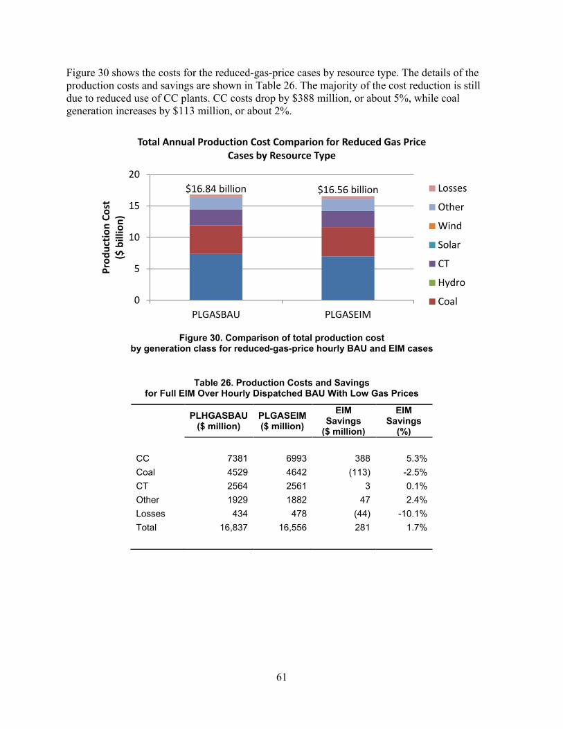
61
Figure 30 shows the costs for the reduced-gas-price cases by resource type. The details of the production costs and savings are shown in Table 26. The majority of the cost reduction is still due to reduced use of CC plants. CC costs drop by $388 million, or about 5%, while coal generation increases by $113 million, or about 2%.
Figure 30. Comparison of total production cost
by generation class for reduced-gas-price hourly BAU and EIM cases
Table 26. Production Costs and Savings
for Full EIM Over Hourly Dispatched BAU With Low Gas Prices
PLHGASBAU
($ million) PLGASEIM ($ million)
EIM Savings
($ million)
EIM Savings
(%)
CC 7381 6993 388 5.3% Coal 4529 4642 (113) -2.5% CT 2564 2561 3 0.1% Other 1929 1882 47 2.4% Losses 434 478 (44) -10.1% Total 16,837 16,556 281 1.7%
$16.84 billion $16.56 billion
0
5
10
15
20
PLGASBAU PLGASEIM
Prod
uctio
n Co
st
($ b
illio
n)
Total Annual Production Cost Comparion for Reduced Gas Price Cases by Resource Type
Losses
Other
Wind
Solar
CT
Hydro
Coal

62
Figure 31 shows the change in energy production by generation class for the low-gas-price cases. The total energy is nearly identical for the BAU and EIM cases. The details are shown in Table 27. CTs and CC plants are reduced—in this case, by a total of about 11 TWh, or 5%—and coal plant production increases by about 11 TWh, or 4%.
Figure 31. Comparison of generation for reduced-gas-price cases
Table 27. Energy Production by Generation Class
for Full EIM Over Hourly Dispatched BAU With Low Gas Prices
PLHGASBAU
(TWh) PLGASEIM
(TWh) EIM Savings
(TWh) EIM
Savings (%)
CC 200 190 11 5.4% Coal 270 281 -11 -4.2% Hydro 254 254 0 -0.1% CT 46 46 0 -0.1% Solar 32 32 0 0.0% Wind 80 80 0 0.0% Other 141 140 1 0.6% Losses 36 36 -1 -1.5% Total 1056 1060 -4 -0.4%
The savings for this low-gas-price sensitivity case (about $281 million annually) are slightly lower than those for the nominal-gas-price case, which were $294 million. One might expect the difference to be larger with lower savings for the reduced-gas-cost case. This is because the overall production costs are lower, and thus the savings should be lower.
0200400600800
10001200
PLGASBAU PLGASEIM
Gen
erat
ion
(T
Wh)
Annual Generation Comparison for Reduced Gas Price Cases
by Resource Type
Losses
Other
Wind
Solar
CT
Hydro

63
There is a larger shift from CC to coal generation in the low-gas-price case than in the nominal-gas-price cases. In the BAU case, the combination of the low gas prices and hurdle rates leads to higher use of CC units—200 TWh versus 187 TWh for the nominal gas price. Remote coal units are displaced by local gas-fired units to a greater extent because average prices for CC generation drop nearly $20/MWh with the lower gas price, making it a more attractive alternative than some remote coal generation with hurdle rates included. Therefore, overall coal use is less than in the nominal-gas-price case.
However, coal use increases more from the low-gas-price BAU case to the low-gas-price EIM than it did in the nominal BAU and EIM cases. As shown in Table 27, coal increases 11 TWh when the EIM is implemented under the low-gas-price scenario. In the nominal-gas-price case, the coal increase was 6 TWh, as shown in Table 21. This occurs because the gas-fired generation is no longer competitive with remote coal generation when the hurdle rates are removed—even at the low gas price. This results in a larger shift to coal for the low-gas-price case. Again, there is still more energy generated by gas in the low-gas case than in the nominal case. It is the increase in coal when implementing the EIM that is greater.
The emissions cases reflect the change in the relative use of gas and coal in the BAU and EIM cases, as shown in Table 28. Carbon is increased in the EIM case because of the shift from gas to coal discussed above.
Table 28. Change in Emissions for Low-Gas-Price Sensitivity Cases
CO2 (ktons)
NOx (ktons)
SO2 (ktons)
PLGASBAU 463,556 668 435 PLGASEIM 470,275 688 448 Increase (ktons) 6719 20 13 Increase (%) 1.4 2.9 2.9
3.5 Reduced-Participation EIM Sensitivity Another sensitivity case was developed to evaluate the impact of reduced participation in the EIM.
The full-EIM footprint includes participation by all BAAs in the Western Interconnection, except those areas with existing markets (CAISO and AESO). The sensitivity case reduced the level of participation by removing BPA and two of the three WAPA BAs. Several PUDs, as well as Seattle City Light and Tacoma Power, are embedded in BPA and, therefore, were also removed from EIM participation in this sensitivity case.
The reduced-participation sensitivity case was first compared with the hourly dispatched BAU case, PLHBAU. This BAU case uses an hourly dispatch with a 40-minute forecast lead time. The reduced-EIM sensitivity case was constrained to use the day-ahead unit commitment from the BAU case. This means all units committed as part of the solution to the hourly BAU case are

64
committed in the EIM. The comparison of these simulations provides the value of the EIM for the reduced-participation case relative to the hourly BAU case.
Table 29 shows the resulting production costs and savings by generation class. The overall production cost savings with reduced EIM participation is $276 million annually, or about 1.4% of total production cost. For comparison, the savings associated with the full EIM was $294 million. The reduced-EIM-participation case produces $18 million less benefit than the full-EIM-participation case.
As in other cases, the savings are dominated by the reduction in CC use, which contributed $321 million, or about 3% of total CC production cost, to the savings. Coal production costs increased by $81 million. Table 30 shows the details of the annual energy production by generation class. The reduction in CC is offset primarily by the increase in coal generation.
Table 29. Production Cost and Savings by Generation Class for Reduced-Participation EIM Over Hourly Dispatched BAU
PLHBAU ($ million)
PLEIM-PMA1
($ million)
EIM Savings
($ million)
EIM Savings
(%)
CC 10,519 10,198 321 3.1% Coal 4,799 4,880 (81) -1.7% CT 3,541 3,542 (1) 0.0% Other 2,121 2,072 49 2.3% Losses 600 612 (12) -2.0% Total 21,580 21,305 276 1.3%
Table 30. Annual Energy Production by Generation Class
for Reduced-Participation EIM Compared With Hourly Dispatched BAU
PLHBAU
(TWh) PLEIM-PMA1 (TWh)
EIM Savings (TWh)
EIM Savings
(%)
CC 187 181 6 3.2% Coal 286 292 -6 -2.2% Hydro 253 254 0 -0.2% CT 43 43 0 -0.3% Solar 32 32 0 0.0% Wind 80 80 0 0.0% Other 143 142 1 0.6% Losses 33 34 -1 -3.1% Total 1056 1060 -4 -0.4%

65
The change in emissions for the hourly BAU and reduced-participation EIM are shown in Table 31. Again, there is an increase because of the increased use of coal, as seen above.
Table 31. Change in Emissions for Hourly Dispatch BAU and Reduced-Participation EIM
CO2 (ktons)
NOx (ktons)
SO2 (ktons)
PLHBAU 473,913 697 461 PLEIM-PMA1 477,530 708 472 Increase (ktons) 3,618 11 11 Increase (%) 0.8 1.6 2.3
The reduced-EIM-participation sensitivity case was also compared with the 10-minute dispatched BAU case, E3BAU. This BAU case uses a 10-minute dispatch with a 10-minute forecast lead time. As in other comparisons, the reduced-EIM sensitivity case was constrained to use the day-ahead unit commitment from the BAU case. This means all units committed for the hourly BAU case are committed in the EIM.
This case comparison gives a lower estimate of savings because the BAU already includes a 10-minute dispatch. The total savings are about $95 million. For comparison, the savings for the full EIM relative to the 10-minute BAU were $146 million. The details of the production costs and savings are shown in Table 32.
Table 32. Production Cost and Changes for Reduced-Participation EIM and 10-Minute Dispatched BAU
E3BAU
($ million) PLEIM-PMA2
($ million)
EIM Savings
($ million)
EIM Savings
(%)
CC 10,547 10,400 146 1.4% Coal 5020 5071 (50) -1.0% CT 2047 2055 (8) -0.4% Other 2061 2046 14 0.7% Losses 593 600 (7) -1.2% Total 20,268 20,173 95 0.5%

66
Table 33 shows that the EIM increases emissions. This is because of the increased use of coal in the EIM case.
Table 33. Change in Emissions for 10-Minute Dispatch BAU and Reduced-Participation EIM
CO2 (ktons)
NOx (ktons)
SO2 (ktons)
E3BAU 478,749 713 483 PLEIM-PMA2 480,740 720 488 Increase (ktons) 1,991 6 6 Increase (%) 0.4 0.9 1.2
3.6 Additional Sensitivity Cases Additional sensitivity analyses of the impact of reduced flexibility reserve requirements and hourly simulation tools were performed. These cases were based on the full-participation EIM.
3.6.1 Reduced Flexibility Reserves Requirements in Economic Dispatch This sensitivity case involved reducing the reserve requirements in the real-time economic dispatch phase of the simulations. The idea is that spinning reserves withheld as part of the unit commitment process could be released during the economic dispatch to compensate for any deviations from schedule.
This sensitivity case is based on the full-EIM case, which uses the 10-minute BAU unit commitment, as described in Section 3.3. This new case differs from the prior case in that only the regulation component of the flexibility reserves is maintained in the economic dispatch. The spinning reserves are released in real time. This scenario represents a potential operating practice. The day-ahead unit commitment ensures that the flex-spin requirements are available in case of a large wind or solar ramp or a deviation from forecast. However, if the flex spin is not needed in real time, there is no reason to keep it, and it can be released to help manage wind and solar variability.

67
Table 34 shows the impact of the reduced reserve requirements on total production cost by comparing the EIM cases with and without the flex-spin component. The reserves reduction saves about $6.9 million of production cost—and about $7.6 million if transmission losses are taken into account.
Table 34. Effect of Reduced Flex Reserve Requirements on Production Cost
Production Cost ($ k)
Cost of Transmission Losses ($ k)
Total Cost ($ k)
EIM case with flex-spin component (PLEIM2) 19,500,959 620,441 20,121,400
EIM case with reduced reserves (PLRES) 19,494,066 619,758 20,113,824
Savings 6893 683 7576
This study did verify that release of the flex spin would not result in significant reserve shortfalls in real time. As such, this sensitivity case demonstrates that the reserve assumptions for the main cases are conservative and some additional savings could be expected if the flex-spin release were done in all cases. The actual result would be different for each EIM case because there is a unique dispatch for each.
3.6.2 Effect of Simulating Short Dispatch Cycles With 1-Hour Time-Step Software
Until recently, no commonly used production simulation software could simulate dispatch periods of less than 1 hour because they all used a 1-hour simulation time-step. Therefore, the WECC-E3 and other studies had to approximate subhourly dispatch by running an hourly time-step simulation with reserve requirements consistent with a 5- or 10-minute dispatch. As discussed Section 3.1, flexibility reserve requirements drop dramatically as the dispatch interval shortens. Hence, these hourly simulations do incorporate some of the effects of fast timing. However, these hourly methods likely understate the effects of intra-hour variability because they cannot account for the extra dispatch movements at the subhourly level. Therefore, they also likely understate production cost.
PLEXOS is a relatively new tool that does have the ability to simulate a subhourly dispatch with a subhourly time-step. As part of the alignment with the WECC-E3 study (Section 3.2), a full-EIM case with10-minute dispatch and 10-minute flexibility reserves was simulated with a 1-hour time-step. A sensitivity case that used a 10-minute time-step was also developed. The same flexibility reserve requirements and unit commitment were used in both cases.

68
Table 35 shows the production cost, cost of transmission losses, and total cost for each case. The 1-hour time-step simulation understated the production cost by about $34 million. Because of a difference in the cost of transmission losses, the understatement of total cost was reduced to slightly more than $17 million.
Table 35. Comparison of Production Costs for 1-Hour Time-Step Simulation Versus 10-Minute Time-Step Simulation of Full EIM
Production Cost ($ k)
Cost of Transmission Losses ($ k)
Total Cost ($ k)
EIM case solved at 1-hour time-step (E3EIM)
19,466,671 637,296 20,103,967
EIM case solved at 10-minute time-step (PLEIM2)
19,500,959 620,441 20,121,400
Increase 34,288 -16,855 17,433
3.7 Comparison of Hourly and 10-Minute BAU Cases Two BAU cases were developed for this study: a 1-hour and a 10-minute dispatch. Until now, comparisons were made between a BAU and an EIM case to estimate savings associated with the EIM. Comparing the two BAU cases is also of interest.
One can think of the 10-minute BAU as a step along the path to the full-EIM implementation in which fast dispatch is adopted before the rest of the EIM. In that sense, movement to the 10-minute BAU represents efficiency improvement, similar to the existing and emerging ITAP, dynamic scheduling system, and ADI. Although these methods are different from a 10-minute dispatch, they qualitatively represent efficiency improvements that would lessen the benefit of an EIM. A comparison of the hourly and 10-minute BAU cases allows the savings associated with the shorter dispatch interval to be separated from those associated with an EIM operating cooperatively across multiple BAAs. In this comparison, all savings are associated with the reduction in reserve requirements and the faster dispatch of the system resources, not the aggregation of variability resulting from an EIM. Section 3.1 showed the reserves for a sample BA decreased 53% on average when operation changed from a 1-hour dispatch with a 40-minute forecast lockdown to a 10-minute dispatch with 10-minute lockdown.
In this sensitivity analysis, the 10-minute and hourly BAU cases were compared. The unit commitment was optimized for each case. This case comparison illustrates the sensitivity of the results to the unit commitment.

69
Table 36 shows the total production costs and savings by generation class for the two BAU cases. The total savings because of the faster dispatch are about $1.3 billion. The savings are primarily from the reduced use of CTs.
Increases in coal generation make up the majority of the energy difference between the two cases, as shown in Table 37. Generation by CTs decreased by 16 TWh annually, and generation by coal increased by 13 TWh.
Table 36. Comparison of Production Costs and Savings by Generation Class for 1-Hour and 10-Minute Dispatched BAU Cases
PLHBAU ($ million)
E3BAU ($ million)
Fast Dispatch Savings
($ million) CC 10,519 10,547 -28 Coal 4799 5020 -221 CT 3541 2047 1494 Other 2121 2061 60 Losses 600 600 0 Total 21,580 20,275 1306
Table 37. Total Energy Production by Generation Class for 1-Hour and 10-Minute Dispatched BAU Cases
PLHBAU (TWh)
E3BAU (TWh)
Fast Dispatch Savings (TWh)
CC 187 189 -2.6 Coal 286 298 -12.6 Hydro 253 254 -0.5 CT 43 26 16.4 Solar 32 32 0.0 Wind 80 80 0.0 Other 143 144 -0.6 Losses 33 35 -1.2 Total 1056 1060 -3.8

70
This comparison shows only the savings associated with the faster dispatch. The total savings from switching to faster dispatch and the EIM can be estimated by comparing the hourly dispatched BAU (PLHBAU) case with the full-EIM case that uses the 10-minute BAU commitment (PLEIM1). This comparison shows a total savings of $1.46 billion. Table 38 shows the production cost by class of generation for these two cases. A comparison of this table and Table 36 shows most of the savings are realized when going from hourly to 10-minute dispatch.
These savings can be compared with the savings associated with the EIM cases discussed in Section 3.3. The EIM using the hourly BAU commitment saw savings of $294 million, and the EIM with the 10-minute BAU commitment saw savings of $146 million.
Table 38. Savings Associated With Fast Dispatch and EIM
PLHBAU ($ million)
PLEIM1 ($ million)
Dispatch and EIM Savings
($ million) CC 10,519 10,357 162 Coal 4799 5067 -268 CT 3541 2051 1490 Other 2121 2026 94 Losses 600 620 -20 Total 21,580 20,122 1458
Table 38 shows the how production changes when change in dispatch is combined with the EIM. CT use drops, with coal and CC generation making up that energy.
Table 39. Approximate Production Savings Associated With Faster Dispatch and EIM
PLHBAU (TWh)
PLEIM1 (TWh)
Dispatch and EIM Savings (TWh)
CC 187 186 1.0 Coal 286 303 -17.4 Hydro 253 254 -0.4 CT 43 26 16.4 Solar 32 32 0.0 Wind 80 80 0.0 Other 143 143 0.4 Losses 33 37 -3.7 Total 1056 1060 -3.8

71
4 Allocation of EIM Benefits to Participants The results presented in the previous section show the overall societal savings associated with an EIM. Additional analysis is required to determine how these benefits would flow to the EIM participants. In the WECC-E3 study, a method was developed to evaluate how those benefits would be allocated. This method was referred to as the Benefits Allocation Roadmap (E3 2011a). The calculations are based on the specific results from the production cost modeling and additional information, such as total load served and generation owned, supplied by the participants.
A number of factors affect the accuracy of roadmap calculations. First and foremost is the fidelity of the production cost model to the actual operations of the Western Interconnection. This study is based on the publicly available WECC TEPPC planning model for the year 2020. There are known limitations to this model—such as the simplification of the trading relationships between the BAs; the use of generic heat rates for generation units; and the inaccuracies inherent in forecasting future load, generation, and transmission system topology. Most of these limitations can be overlooked because the analysis compares two similar cases at a macro scale. These issues and how they affect the outcome are discussed in detail in the report from the WECC-E3 EIM benefits analysis study (E3 2011c).
A critical factor in understanding the allocation of EIM benefits to the participants is the omission of bilateral contract information in the model. Lack of contractual data has a significant impact on the commitment and dispatch performed by the model. In all the EIM and BAU cases that were modeled and analyzed, PLEXOS minimized production cost subject to the many constraints imposed by unit operating limits, transmission limits, and other inputs and did not consider contracts between entities in the West because that information was not available. Therefore, the individual benefits presented below are based on an optimal dispatch of the BAU and EIM cases.
Individual BAs can potentially refine these allocation results significantly. For example, if a BA has contractual obligations to sell given amounts of energy during a year at a specified price, the revenue from those sales will not be affected by potential EIM transactions. Likewise, if a BA holds contracts for purchases at a specified price, the EIM would have no impact on that cost. Thus, individual BAs would likely have the ability to post-process the modeling data to account for bilateral and other contractual mechanisms that are not part of the model.
4.1 Allocation Method The method developed for the WECC-E3 EIM benefits study has its roots in even earlier work. Similar methods were used in the Cost Benefits Analysis for the Southwest Power Pool (2005) and, to some extent, in the Eastern Wind Integration and Transmission Study’s (2010) Adjusted Production Cost.
The goal of the allocation procedure is to fairly allocate the savings (or cost) incurred because of the implementation of an EIM. The first thought might be to just determine the change in production costs for each participant. There is more to the story, however. The implementation of an EIM results in changes in the import and export of energy between the participants. One participant may generate and export more energy in the EIM case than in the base case. Therefore, the increased production costs are due to the extra energy sold as well as to the EIM.

72
Similarly, a participant may import more energy under an EIM. Its production cost is reduced, but it is also purchasing more energy. The allocation procedure must account for energy sales and purchases as well as production costs.
The approach used in the referenced studies has been called modified generation cost or adjusted production cost, which is used in this report. The idea is to calculate the cost of serving participants’ load by netting out transactions and valuing imports and exports in such a way as to determine an effective production cost.
To properly value imports and exports, some pricing mechanism is necessary. The PLEXOS model economically dispatched generation and recorded prices at each node of the system. These are called locational marginal prices, or LMPs. Although the West does not use LMPs, the basic calculation of LMPs by PLEXOS provides a good way to represent the value of energy imports and exports4.
The adjusted production cost for a BA is calculated as:
adjusted production cost = prorated production cost for all units owned or contracted by the BA
+ net imports priced at load-weighted LMP - Net exports priced at generation-weighted LMP.
Production costs are calculated as the sum of prorated production costs for units owned or contracted by the BA, including units that are remote from the BAA but whose output is partially or fully owned or contracted by the BA. It also includes partially owned units within the BAA boundaries. The ownership information was primarily derived from the TEPPC 2020 PC0 model, with additional ownership information obtained from Energy Information Administration Form 860 (2010) and stakeholders. Net imports and exports are calculated each interval (1-hour or 10-minute) by determining the total generation associated with the BA and subtracting the total load responsibility of the BA. If the difference is positive, then excess energy is available in the BA, and it is sold at that interval’s generator-weighted LMP for the BA. If the difference is negative, there is less generation than required, and the difference is purchased at that interval’s load-weighted LMP for the BA. The load- and generation-weighted LMPs are calculated for each BA in each interval from the production simulation results.
The value of transmission losses must also be added to the above components because the generator production costs do not include these losses. The value of the losses is calculated by obtaining an interval’s (hour or 10-minute) losses for all transmission at 115 kV and above and pricing them at the interval’s average production cost for the area that owns the transmission.
4 LMPs are used solely to illustrate simulation results. Although LMPs are also used in the operation of centrally organized electricity markets (e.g., regional transmission organizations and ISOs), the use of LMPs in this report does not imply the need for a regional transmission organization in the West.

73
Similar to the societal saving calculations, the adjusted production costs for each BA were calculated first for the BAU case and then for the EIM case. The allocated savings are the differences between the EIM and BAU adjusted production costs for each BA. In the following sections, each component of the adjusted production cost is calculated individually to illuminate the nature of the savings for each BA.
4.2 Allocation of Benefits for EIM Under Hourly BAU The allocation of benefits for the hourly dispatched BAU and full-EIM case pair (presented in Section 3.3.1) is discussed in this section. The BAU case uses an hourly dispatch, with a forecast that is set 40 minutes prior to the beginning of the hour. All BAAs in the Western Interconnection participate in the EIM except those with existing markets (i.e., CAISO and AESO).
The allocation of benefits for all EIM participants is shown in Table 40. For each BA, the change in production cost, purchases, and exports as well as the adjusted production cost savings is shown. Savings are indicated by positive numbers, and cost increases are negative. Imports are reported as positive for reductions in import costs. Exports are reported as positive for increases in revenue. For instance, AZPS has a $27-million reduction in production cost for all generation, $14 million in additional purchases of energy, and $12 million less in export revenue. This results in a total adjusted production cost savings of $0.8 million. Avista has a $4.5-million reduction in production cost, $33.6 million less in import costs, and an $87-thousand increase in export revenue. This results in a total adjusted production cost savings of $38 million.

74
Table 40. Allocation of EIM Benefits (With the Hourly BAU Unit Commitment) to EIM Participants
Reduction in Production Cost ($ k)
Decrease in Import Cost
($ k)
Increase in Export
Revenue ($ k)
Adjusted Production
Cost Savings ($ k)
APS 27,000 (14,000) (12,000) 1,000 AVA 5000 34,000 0 38,000 BCTC 6500 (4600) (27,900) (26,100) BPA 40,900 0 (354,100) (313,300) CHPD 0 (1500) (7900) (9400) DOPD 0 (1200) (2700) (4,000) EPE 12,800 (2700) (1300) 8700 GCPD 0 2500 (4500) (1900) IID 2400 (100) (16,900) (14,500) IPC (2,300) 3400 (3000) (1900) LADWP 20,400 32,300 (3500) 49,200 NEVP 33,500 (10,100) (17,000) 6300 NWE (23,600) 6200 41,100 23,700 PACE (97,300) 19,500 156,800 79,000 PACW 10,800 49,200 100 60,000 PGN 11,100 64,600 0 75,700 PNM (13,000) 800 17,600 5500 PSCO 39,700 46,600 6600 92,900 PSE (10,300) 107,600 300 97,500 SCL 0 24,300 (200) 24,100 SMUD 28,700 10,900 0 39,600 SPPC 10,300 10,500 (100) 20,600 SRP 51,900 4600 0 56,500 TEP 13,200 7000 (4600) 15,600 TID 3800 7500 0 11,300 TPWR 0 8800 (500) 8300 WACM (6500) 3000 3900 400 WALC 11,000 (100) (32,100) (21,200) WAUM 0 0 7400 7400

75
The high reserve requirements of these cases lead to significant CT commitment to cover the flexibility needs of the BAAs. This is particularly true for BAAs with high solar penetration because those requirements are relatively more demanding. This leads to significant out-of-merit-order commitment because high-cost CTs are frequently not needed for energy because lower-cost units are available. They are committed and running at minimum generation only to provide necessary reserves. Because the day-ahead commitment decisions of the SCUC must be honored in the EIM to be sure the BAs are capable of self-sufficiency, those CTs remain committed in the EIM, which limits the savings possible in many BAAs. If these CTs were instead taken offline when not needed, and started when needed, then the results could change significantly.
There are several patterns in the results. First, there are BAs whose production costs are cut substantially because of the reduction of reserve requirements and the use of more-economical resources without significantly changing imports or exports. SRP is an example of this. Its production costs are reduced by $52 million with the EIM. A relatively small decrease in both import costs and export revenue leaves it with a net benefit of $56 million.
Next, there are BAs with low-cost coal resources that increase exports with the reduced transactional friction between BAs in the EIM case. PACE is an example of this. Its production costs increase by $97 million, but its export revenues increase by $157 million. This results in an overall savings from the EIM of $79 million.
Another group of BAs sees decreases in production costs but increases in imports and/or decreases in export revenues. Typically, these are BAs with high renewable energy penetration levels that benefit from the reduced EIM reserve requirements. APS is a good example of such a BA. Its production cost is reduced by $27 million, purchases increase by $14 million, and sales decrease by $12 million. The net benefit to the BA is $1 million.
Yet another group has relatively small changes in production cost but relatively large savings on purchased energy. The purchased energy savings are due to the reduction in overall LMPs across most of the Western Interconnection with the EIM. These BAs tend to be smaller areas that import a significant amount of their energy. PGN is an example. There is a reduction of $11 million in production cost but a larger decrease in purchases of $65 million. This gives a total savings of $76 million. SMUD also falls into this category, with a reduction of $29 million in production costs and $11 million in energy purchase costs, even though it imports an additional 250 GWh in the EIM case.
Finally, there are BAs that see small benefits or penalties to production cost but large decreases in export revenue. BPA is an example of this group. The value of BPA’s exports decline because of the overall decrease in LMP throughout the Western Interconnection and a slight rise in generator-weighted LMP in BPA. The value of the exports decreases by $354 million, while production cost savings are $40 million. This results in a net increase in costs of $314 million.
The EIM also impacts nonparticipants, such as the CAISO utilities, AESO, and CFE. Table 41 shows the results of the benefits allocation roadmap for those entities.

76
Table 41. Allocation of EIM Benefits (With the Hourly BAU Unit Commitment) to EIM Nonparticipants
Reduction in Production Cost ($ k)
Decrease in Import Cost
($ k)
Increase in Export
Revenue ($ k)
Adjusted Production
Cost Savings ($ k)
AESO (9100) (9400) (700) (19,200) CFE 7700 (4900) (2200) 600 PGE 43,200 63,000 (11,700) 94,600 SCE 45,100 60,000 (6200) 98,900 SDGE 17,200 12,700 (6500) 23,400
About 60% of the societal benefit calculated as the production cost savings for the EIM belongs to the participants of the EIM. The other 40% is realized by nonparticipants, such as the CAISO utilities and AESO. To understand why such large benefits go to nonparticipants, it is important to understand that all entities are going from a 1-hour to a 10-minute dispatch interval. Therefore, they also see the benefits of faster schedules. Areas such as CAISO are also able to import more energy under the EIM at prices well below that of the CTs needed for the BAU flexibility reserve requirements.
SCE, for instance, sees a $45 million reduction in production costs when 10-minute dispatch is implemented. This is primarily because of a reduction in CC use—about $35 million representing about 644 GWh of energy. There are also reductions in coal, biomass, and steam generation totaling 416 GWh. This results in an additional production cost savings of $14 million. The energy is replaced through additional purchases and reduced sales of approximately 1100 GWh for an additional savings of $60 million. This is possible because the price paid for all purchased energy falls by about $5/MWh on average.
To understand the factors driving the changes in generation patterns, it is useful to consider the LMP for the entire Western Interconnection and observe the LMP-driven flows between the BAs. To visualize this data, an LMP map was developed. Each map has a background that shows the average annual bus LMPs across the Western Interconnection, where the colors indicate the value of the LMP. These plots are frequently called “heat maps” because the color tells the “temperature” of the variable being plotted. For the annual average LMP, cooler colors indicate lower LMPs, and warmer colors indicate higher LMPs. The color scales and associated LMP values are shown on each plot.
On top of the LMP map are bubbles for each BA in the PLEXOS model. The arrows between the bubbles indicate the average hourly power flows between BAs. The width of the arrows is a coarse indication of the magnitude of the flow and gives a sense of the big picture. The detailed flow data are on top of the arrows. For clarity, flows between BAs of less than 100 MW are not shown.

77
Figure 32 shows the LMP map for the hourly BAU (PLHBAU) case. The LMPs are highest in California, with an average near $50/MWh. LMPs are lowest in the northeastern part of the Western Interconnection, with an average in the low $20s/MWh in NWE. Elsewhere, the prices tend to be in the mid-$30s/MWh. There is a clear pattern of energy moving from low- to high-price areas, with movement generally from east to west and north to south.
Figure 32. LMP map for hourly BAU case
The average generator-weighted and load-weighted LMPs for each of the BAs are shown in Table 42 for the hourly dispatched BAU case. The highest prices are seen in BANC, NEVP, and PSC. The lowest prices are seen in NWMT, WACM, and PACE. NWMT has low LMP because of the hydro, wind, and coal facilities.
1-Hour BAU LMP($/MWh)
55504540353025
BCTC AESO
NWE
AVA
BPA
PSE
PGE
PACW
BANC
CAISO
LADWP
IID
WACM
PSCO
WALC
IPC
PACE
APS
TEP
SRP
PNM
EPE
NEVP
891
626
178
1181
607
1111
SPP
153
602100
116
105
891
179
857
777 2633
393
216
1139
2274840
705
324
489
113
431261
386
788
197265
718
492
560
204
Hourly BAUAnnual Average Nodal LMPAnd Regional Flows above
100MWThickness of lines indicates magnitude of
flow
173
101

78
Table 42. Average Weighted LMP for Hourly BAU Case
Area Generation-Weighted
LMP ($/MWh)
Load-Weighted
LMP ($/MWh)
Area Generation-Weighted
LMP ($/MWh)
Load-Weighted
LMP ($/MWh)
AESO 55.69 60.61 PGE 49.26 49.32 APS 32.82 33.30 PGN 36.16 38.49 AVA 31.61 34.51 PNM 31.79 32.32 BCTC 39.37 39.13 PSCO 39.91 41.09 BPA 35.20 35.73 PSE 33.84 39.62 CFE 51.32 51.32 SCE 45.65 48.20 CHPD 35.35 35.32 SCL 29.19 36.21 DOPD 35.35 35.24 SDGE 45.29 45.80 EPE 35.48 37.86 SMUD 47.91 48.21 GCPD 35.20 35.18 SPPC 38.48 38.46 IID 39.89 40.47 SRP 34.45 34.85 IPC 31.04 31.58 TEP 33.47 33.56 LADWP 41.09 43.10 TID 48.31 48.31 NEVP 43.22 44.48 TPWR 35.69 35.94 NWMT 21.05 20.40 WACM 27.98 27.81 PACE 27.79 27.98 WALC 35.79 35.71 PACW 35.46 37.10 WAUM 20.50 22.40
As shown in Figure 33, the effect of the full EIM is to reduce the range of LMPs across the Western Interconnection, raising the price in low-cost generation regions and lowering the price in others. The color scale is identical to the previous plot of the BAU case. Significantly higher prices are observed in NWE and, to a lesser extent, PACE and WACM. Table 43 shows the average generator-weighted and load-weighted LMP values for each area.

79
Figure 33. LMP map for full-EIM case with hourly BAU unit commitment
Table 43. Average Weighted LMP for Full-EIM Case With Hourly BAU Unit Commitment
Area Generation-Weighted
LMP ($/MWh)
Load-Weighted
LMP ($/MWh)
Area Generation-Weighted
LMP ($/MWh)
Load-Weighted
LMP ($/MWh)
AESO 55.79 60.69 PGE 44.52 44.62 APS 30.43 30.96 PGN 30.17 30.91 AVA 26.39 26.36 PNM 30.32 30.06 BCTC 37.31 37.00 PSCO 29.55 29.54 BPA 30.47 31.11 PSE 30.74 32.22 CFE 50.12 50.12 SCE 41.25 43.41 CHPD 30.95 30.92 SCL 25.58 32.05 DOPD 30.95 30.80 SDGE 40.80 41.23 EPE 31.18 31.66 SMUD 40.95 41.96 GCPD 30.72 30.71 SPPC 31.28 31.37 IID 36.01 36.33 SRP 31.36 30.80 IPC 30.33 30.42 TEP 30.85 30.72 LADWP 31.76 37.12 TID 42.47 42.47 NEVP 37.59 38.42 TPWR 31.23 31.65 NWMT 27.33 27.21 WACM 29.50 29.44 PACE 29.81 30.11 WALC 33.38 32.89 PACW 30.46 30.87 WAUM 27.58 28.72
Full EIM with 1-Hour BAU LMP($/MWh)
55504540353025
BCTC AESO
NWE
AVA
BPA
PSE
PGE
PACW
BANC
CAISO
LADWP
IID
WACM
PSCO
WALC
IPC
PACE
APS
TEP
SRP
PNM
EPE
NEVP
839
615
116
1384
623
1463
238
SPP
182
775
181
102
864
182
857
911 2098
1124
1138
22731222
701
925
117
556
198
132
471353
447
817
178
187288
854
464
486
314
Case PLEIM with 1-Hr BAUAnnual Average Nodal LMPAnd Regional Flows above
100MWThickness of lines indicates magnitude of
flow
128
150

80
Figure 34 shows both the change in LMPs and the change in flows between the EIM and BAU cases. The color scale indicates the increase or decrease in the LMPs associated with the implementation of the EIM. Only power flow changes of more than 50 MW are shown. Flows that decrease are in red. In general, the flow increases from east to west. It follows both the low-to-high LMP differential and the removal of hurdle rates in the EIM case.
Although the average flow directly from BPA to CAISO decreases by 549 MW, that flow is made up with additional flow from BPA through LADWP and BANC. This is because the hurdle rate from BPA to CAISO is $11.44, while that from LADWP to CAISO is $9.68 and from BANC to CAISO is $5.99. With the EIM in place, there are no hurdle rates from BPA to either LADWP or BANC, which makes these paths less expensive. In addition, significant energy comes in from NEVP, which also has a lower hurdle rate at $8.03 than the BPA path.
Figure 34. LMP map of LMP changes from hourly BAU to full EIM with hourly unit commitment
Table 44 shows the change in annual average generator-weighted and load-weighted LMP values for each area. As shown in Figure 34, the largest changes are in the low-cost northeastern areas of NWE, PACE, and WACM. Without the EIM, these areas have long periods with very low LMP values because of large amounts of wind. With the EIM, more energy can move out of the northeastern region, which reduces the time when LMPs are below the marginal costs of the lowest-cost thermal generators in the region. In NWE, the LMP is below the marginal cost for Colstrip for about 2800 hours/year in the BAU case and around 1200 hours in the EIM case.
Change in LMP ($/MWh)1-Hour BAU to Full EIM
20151050
-5-10
BCTC AESO
NWE
AVA
BPA
PSE
PGE
PACW
BANC
CAISO
LADWP
IID
WACM
PSCO
WALC
IPC
PACE
APS
TEP
SRP
PNM
EPE
NEVP
-63
203
68
106
352
186
SPP
88
81
-88
134 -535
732
382
64
601
67
103
92
136
-74
110
FULL EIM Compared to Hourly BAUAnnual Average Nodal LMP Changes
And Regional Flows Increases above 50 MWThickness of lines indicates magnitude of change of flow
Red lines indicate reduction of flow in EIM Case
81
173
-52
-155
173
72

81
Table 44. Average Weighted LMP Changes From Hourly BAU to Full EIM With Hourly Unit Commitment
Area Generation-Weighted
LMP ($/MWh)
Load-Weighted
LMP ($/MWh)
Area Generation-Weighted
LMP ($/MWh)
Load-Weighted
LMP ($/MWh)
AESO 0.10 0.08 PGE -4.74 -4.70 APS -2.39 -2.34 PGN -5.99 -7.58 AVA -5.22 -8.16 PNM -1.47 -2.26 BCTC -2.06 -2.13 PSCO -10.36 -11.55 BPA -4.74 -4.62 PSE -3.10 -7.40 CFE -1.20 -1.20 SCE -4.40 -4.79 CHPD -4.40 -4.41 SCL -3.61 -4.15 DOPD -4.40 -4.44 SDGE -4.49 -4.57 EPE -4.31 -6.20 SMUD -6.97 -6.25 GCPD -4.48 -4.47 SPPC -7.20 -7.08 IID -3.87 -4.14 SRP -3.10 -4.05 IPC -0.72 -1.16 TEP -2.62 -2.84 LADWP -9.33 -5.98 TID -5.83 -5.83 NEVP -5.63 -6.05 TPWR -4.46 -4.29 NWMT 6.28 6.81 WACM 1.53 1.64 PACE 2.01 2.13 WALC -2.41 -2.82 PACW -5.00 -6.23 WAUM 7.08 6.32
PSCO has a significant reduction in LMP because of the reduction of reserve requirements and the removal of hurdle rates to allow additional imports from WACM.
The effect of the EIM is less noticeable in the southwest (APS, PNM, and SRP), where significant amounts of CTs are committed and running to cover the high reserve requirements associated with the high penetration of solar resources. For example, there are approximately 100,000 hours of CT operation, mostly at minimum generation, in APS for both the hourly BAU and EIM cases. Note that the EIM case was constrained to use the hourly BAU commitment. Therefore, running high-cost resources at minimum generation limits the ability of the BA to find lower-cost energy from neighbors even with hurdle rates eliminated in the EIM. An improved model of quick-start CTs would allow these units to start and stop during real time rather than maintaining the day-ahead commitment and enforcing minimum generation.
LADWP sees a sizable reduction in LMP because of its relatively high LMP in the BAU case and the new resources available at much lower cost when hurdle rates are removed in the EIM case. As shown in Figure 34, flows from BPA and the southwestern BAs into LADWP increase with the EIM.

82
4.3 Allocation of Benefits for EIM Compared With the 10-Minute BAU The allocation of benefits for the 10-minute dispatched BAU and full-EIM case pair (presented in Section 2.4.2) is discussed in this section. The BAU case uses a 10-minute dispatch with a forecast that is set 10 minutes prior to the beginning of a dispatch interval. All BAs in the Western Interconnection participate in the EIM except those with existing markets (i.e., CAISO and AESO). The changes from a 10-minute BAU to the EIM are likely to be more modest than for the hourly BAU because the savings associated with reserve reductions are much smaller. With the lower reserves in the 10-minute dispatch BAU case, the largest differences would be expected for BAs with higher variable generation penetrations and thus higher reserve requirements.
The allocation results for this pair of cases are shown in Table 45. Savings are indicated by positive numbers, and cost increases are negative. Imports are reported as positive for reductions in import costs. Exports are reported as positive for increases in revenue.
The reductions in production costs are primarily due to the reduction of reserve requirements with the EIM. Also, there are additional exchanges of energy from lower-cost areas to higher-cost areas because of the elimination of hurdle rates in the EIM and the accompanying general reduction in LMP.
Several patterns are evident in the results. The largest group sees small to moderate changes in production cost but a substantial reduction in purchased energy cost. This is because of a general lowering of prices across most of the Western Interconnection. PGN, PSE, and AVA are typical of this group. They tend to have fairly low levels of variable generation in their portfolios and import significant amounts of their energy requirements.
A group of BAs (NWE, PACE, and WACM) sees production cost rise because its members are low-cost producers and export more energy when hurdle rates are removed. The additional export revenues more than offset the increase in production cost, giving a net savings with the EIM.
PSCO and LADWP are examples of BAs that have lower production costs primarily because of the reduction of reserve requirements from the EIM. These BAs have significant variable generation assigned to their territories. The pooling in the EIM of variability from that variable generation leads to the reduction. They are also able to purchase additional energy in the EIM because of the elimination of hurdle rates with their neighbors.
PNM is typical of a group that sees relatively small change in production cost. In PNM’s case, there is a small increase in production cost because of an increase in exports. This increase in exports occurs because of the removal of hurdle rates with the EIM.

83
Table 45. Allocation of EIM Benefits (With the 10-Minute BAU Unit Commitment) to EIM Participants
Reduction in Production Cost ($ k)
Decrease in Import Cost ($
k)
Increase in Export
Revenue ($ k)
Adjusted Production
Cost Savings ($ k)
APS 10,400 6700 1500 18,700 AVA 1800 22,100 200 24,000 BCTC 2900 (7500) 8600 4000 BPA 31,500 0 (206,600) (175,000) CHPD 0 0 (5200) (5100) DOPD 0 (400) (2000) (2400) EPE 11,600 (4800) (700) 6000 GCPD 0 1100 (2500) (1,300) IID 400 0 (5600) (5300) IPC (5700) 2100 7200 3600 LADWP 13,700 16,100 (400) 29,400 NEVP 8000 9300 6500 23,700 NWE (19,200) 3800 42,200 26,800 PACE (59,500) 8900 144,700 94,200 PACW 4100 28,500 100 32,700 PGN 10,000 41,900 0 51,900 PNM (7200) 3000 16,400 12,200 PSCO 38,400 29,200 3300 70,900 PSE (9100) 77,000 400 68,300 SCL 0 11,800 100 11,900 SMUD 16,500 4900 (200) 21,200 SPPC 6800 6300 (100) 13,100 SRP 32,400 10,500 0 42,900 TEP 0 7900 10,200 18,100 TID 3500 2000 0 5400 TPWR 0 4100 (100) 4000 WACM (17,500) 9500 13,400 5400 WALC (3500) 0 3400 (100) WAUM 0 0 10,600 10,600
Table 46 shows the allocation of benefits for BAs not participating in the EIM. As with the participant benefits, there is generally a decline in these benefits compared with the hourly dispatch case. Unlike the hourly dispatch case, in which the majority of savings were due to the reduction in reserve requirements in areas with substantial variable generation, the savings here are primarily due to the general lowering in the cost of energy throughout the Western Interconnection.

84
Table 46. Allocation of EIM Benefits (With the 10-Minute BAU Unit Commitment) to EIM Nonparticipants
Reduction in Production
Cost ($ k)
Decrease in Import Cost
($ k)
Increase in Export
Revenue ($ k)
Adjusted Production
Cost Savings ($ k)
AESO (25,600) 41,600 200 16,200 CFE 8000 (9000) (2700) (3800) PGE 30,100 52,900 (4800) 78,100 SCE 39,200 19,100 (2100) 56,300 SDGE 23,700 2900 (5500) 21,100
The LMP map for the 10-minute BAU (E3BAU) case is shown in Figure 35. (A description of this type of figure and its interpretation is in Section 4.2.) It looks similar to the hourly BAU (PLHBAU) shown in Figure 32 and discussed in the previous section. However, a comparison of these two figures shows that the LMP values are higher in the 10-minute BAU than in the hourly BAU. In fact, they are higher in nearly every BA by about $6/MWh on average. Although it seems backward, the hourly BAU has lower LMPs because of the out-of-merit-order commitment of CTs to cover flex reserve requirements. There are enough CTs running at minimum load to push down the loading on more-efficient generators, making those the marginal units.
Figure 35. LMP map for 10-minute BAU case
Full EIM with 10-Min BAU LMP($/MWh)
55504540353025
BCTC AESO
NWE
AVA
BPA
PSE
PGE
PACW
BANC
CAISO
LADWP
IID
WACM
PSCO
WALC
IPC
PACE
APS
TEP
SRP
PNM
EPE
NEVP
937
648
223
844
632
1318
SPP
140
715124
107
862
216
832
843 2997
478
1049
2263967
647
322
444
181
111
245311
383
778
357326
730
371
613
276
Case E3BAU with 10-Minute BAUAnnual Average Nodal LMPAnd Regional Flows above
100MWThickness of lines indicates magnitude of
flow
105
107
114
161
174

85
Flows between BAs are, in general, a bit lower in the hourly dispatch case. This is because each BA has higher reserve requirements in the 1-hour case, which forces more units to be committed locally. In the 10-minute case with lower reserve requirements, fewer high-cost units are committed, and a more optimal dispatch is possible.
Table 47 shows annual average generation-weighted and load-weighted LMP values for each of the study areas. Again, NWMT, PACE, IPC, WAUM, and WACM show the lowest average LMPs because of the mix of low-cost generation such as coal, hydro, and wind compared with the relatively low load levels found in these areas. The highest U.S. prices are found in PG&E at $53/MWh and BANC at $51/MWh.
Table 47. Average Weighted LMP for 10-Minute BAU Case
Area Generation-Weighted
LMP ($/MWh)
Load-Weighted
LMP ($/MWh)
Area Generation-Weighted
LMP ($/MWh)
Load-Weighted
LMP ($/MWh)
AESO 56.11 60.92 PGE 53.26 53.34 APS 38.39 38.67 PGN 37.77 40.28 AVA 33.13 36.31 PNM 36.53 36.94 BCTC 41.40 41.15 PSCO 41.71 42.92 BPA 37.08 37.67 PSE 35.38 41.55 CFE 54.48 54.46 SCE 49.63 52.12 CHPD 37.25 37.22 SCL 30.21 38.13 DOPD 37.24 37.14 SDGE 49.89 50.30 EPE 41.35 44.05 SMUD 50.62 50.98 GCPD 37.09 37.08 SPPC 40.64 40.63 IID 44.39 45.06 SRP 38.97 40.03 IPC 32.28 32.81 TEP 37.89 38.26 LADWP 44.64 46.35 TID 51.11 51.11 NEVP 46.83 48.31 TPWR 37.61 37.86 NWMT 21.94 21.42 WACM 29.34 29.15 PACE 28.91 29.08 WALC 39.73 39.82 PACW 36.50 38.21 WAUM 21.53 23.42
Figure 36 shows the LMP map and major energy flows for the EIM case with the 10-minute BAU commitment. The effect of the EIM is to even out the LMPs across the Western Interconnection by raising the price in low-cost generation regions and lowering the price in others. The color scale is identical to the previous plot of the BAU case. Note the significantly higher prices in NWE and WAUM and, to a lesser extent, PACE, WACM, and IPC. Table 48 shows the average generator-weighted and load-weighted LMP values for each area.

86
Figure 36. LMP map for full-EIM case with 10-minute BAU unit commitment
Table 48. Average Weighted LMP for Full-EIM Case With 10-Minute BAU Unit Commitment
Area Generation-Weighted
LMP ($/MWh)
Load-Weighted
LMP ($/MWh)
Area Generation-Weighted
LMP ($/MWh)
Load-Weighted
LMP ($/MWh)
AESO 56.78 61.50 PGE 51.19 51.27 APS 37.25 37.47 PGN 34.41 35.12 AVA 30.76 30.83 PNM 36.42 36.09 BCTC 40.92 40.63 PSCO 34.69 34.65 BPA 34.74 35.31 PSE 34.91 36.36 CFE 55.71 55.69 SCE 47.60 49.86 CHPD 35.19 35.13 SCL 29.20 36.20 DOPD 35.19 35.02 SDGE 47.35 47.77 EPE 38.57 39.83 SMUD 46.58 47.69 GCPD 34.97 34.93 SPPC 36.18 36.24 IID 42.54 42.86 SRP 37.69 37.37 IPC 34.80 34.85 TEP 37.37 37.40 LADWP 36.97 43.05 TID 48.26 48.23 NEVP 43.45 44.40 TPWR 35.45 35.82 NWMT 31.58 31.46 WACM 34.57 34.47 PACE 34.46 34.65 WALC 39.71 39.30 PACW 34.72 35.10 WAUM 31.87 32.81
Full EIM with 10-Min BAU LMP($/MWh)
55504540353025
BCTC AESO
NWE
AVA
BPA
PSE
PGE
PACW
BANC
CAISO
LADWP
IID
WACM
PSCO
WALC
IPC
PACE
APS
TEP
SRP
PNM
EPE
NEVP
923
663
181
953
651
128
102
1503
249
SPP
176
816
177
108
813
249
847
949 2352
1173
1083
22691243
169
658
956
125
529
249
131
265363
439
843
185
361376
870
373
541
330
Full EIM with 10-Min BAUAnnual Average Nodal LMPAnd Regional Flows above
100MWThickness of lines indicates magnitude of
flow
121
102

87
Figure 37 shows the change in LMPs and average flows between BAAs between the 10-minute BAU case and the EIM case. Black lines show flows that increase with the EIM, and red lines indicated flows that decrease. The thickness of the lines roughly indicates the magnitude of the change in flow. Again, flow increases from the northeastern section of the Western Interconnection to the west and southwest. This indicates that lower-cost energy is flowing from areas of lower costs to areas of higher with the removal of hurdle rates with the EIM. There is a large decrease in sales from BPA to CAISO. This energy is made up through smaller increases in flows from a number of BAAs. This happens because the hurdle rate from BPA to CAISO is $11.44—higher than the hurdle rates from other BAAs.
Figure 37. LMP map of LMP changes from 10-minute BAU
to full EIM with 10-minute unit commitment
As in the hourly dispatch case, nearly all BAs see lower LMPs with the EIM. The exceptions are the low-cost areas of NWMT, PACE, IPC, and WACM. These areas see substantial increases in LMP values. Table 49 shows the change in LMP values for each area from the 10-minute BAU case to the EIM case.
Change in LMP ($/MWh)10-Min BAU to Full EIM
20151050
-5-10
BCTC AESO
NWE
AVA
BPA
PSE
PGE
PACW
BANC
CAISO
LADWP
IID
WACM
PSCO
WALC
IPC
PACE
APS
TEP
SRP
PNM
EPE
NEVP
109
58
185
181
SPP
74
53
107 -645
696
202276
64
634
85
56
52
65
50
140
-72
54
Full EIM compared to 10-Minute BAUAnnual Average Nodal LMP Changes
And Regional Flows Increases above 50 MWThickness of lines indicates magnitude of change of flow
Red lines indicate reduction of flow in EIM Case
77
78
-93 101
56
50

88
Table 49. Average Load-Weighted LMP Changes From 10-Minute BAU to Full EIM With 10-Minute Unit Commitment
Area Generation-Weighted
LMP ($/MWh)
Load-Weighted
LMP ($/MWh)
Area Generation-Weighted
LMP ($/MWh)
Load-Weighted
LMP ($/MWh)
AESO 0.67 0.57 PGE -2.07 -2.07 APS -1.15 -1.19 PGN -3.35 -5.16 AVA -2.37 -5.47 PNM -0.11 -0.85 BCTC -0.48 -0.52 PSCO -7.03 -8.26 BPA -2.34 -2.35 PSE -0.47 -5.19 CFE 1.23 1.23 SCE -2.03 -2.25 CHPD -2.06 -2.09 SCL -1.01 -1.93 DOPD -2.06 -2.12 SDGE -2.54 -2.52 EPE -2.78 -4.23 SMUD -4.03 -3.28 GCPD -2.12 -2.14 SPPC -4.46 -4.39 IID -1.85 -2.19 SRP -1.28 -2.67 IPC 2.52 2.04 TEP -0.52 -0.86 LADWP -7.67 -3.30 TID -2.85 -2.88 NEVP -3.38 -3.91 TPWR -2.16 -2.04 NWMT 9.64 10.04 WACM 5.23 5.31 PACE 5.54 5.58 WALC -0.02 -0.51 PACW -1.79 -3.11 WAUM 10.34 9.39
5 Conclusions This study was performed at the request of the Western Interstate Energy Board’s PUC EIM working group. The primary objective of the analysis was to build upon prior work by WECC and E3 to further evaluate the potential benefits of an EIM.
Any study, including this one, necessarily involves assumptions and approximations to compensate for missing data, software limitations, and the inherent uncertainty of the future. Modeling any large system, especially one with the physical characteristics and existing market relationships of the Western Interconnection, is complex and difficult. One set of study assumptions and modeling approximations, as described in Section 2, was used in this study to represent the key elements of the BAU and EIM study scenarios. Other assumptions and approximations could be analyzed in future studies. Therefore, the results of this study represent a possible outcome rather than a definitive forecast. Flexibility reserve requirements, societal (system-wide) benefits, and individual BAA results were calculated.
Flexibility reserves are in addition to, not instead of, existing contingency reserve requirements and are intended to help manage wind, solar, and load variability. This additional reserve requirement is a function of the time-synchronized expected variability of wind and solar power, which is, in turn, a function of the wind and solar output. For example, if wind power output is at

89
or near maximum, then there is relatively little variability and, therefore, relatively small flexibility reserve requirements. Conversely, if wind power output is in the middle of the operating range, then its variability is higher and the flexibility reserve requirements are higher. The flex reserve requirements decrease with shorter dispatch interval/forecast lockdown times and with larger EIM participation.
This study shows an annual societal operating benefit of between $146 million and $300 million for the EIM with full participation. There is an additional benefit of approximately $1.3 billion associated with moving from an hourly dispatch interval to a 10-minute dispatch interval. Some of these large benefits may be achieved through implementation of Federal Energy Regulatory Commission Order 764 as well. Therefore, the total benefit of a faster dispatch interval and shared flexibility reserves could be as high as $1.46 billion.
Table 50. Summary of EIM Savings
Case Savings ($ millions)
Full EIM with hourly BAU commitment compared with hourly BAU 294
Full EIM with 10-min BAU commitment compared with 10-minute BAU 146
Reduced EIM with hourly BAU commitment compared with hourly BAU 276 Reduced EIM with 10-minute BAU commitment compared with 10-minute BAU 95 Lower-gas price, full EIM with hourly BAU commitment compared with hourly BAU 281 Reduced-reserve, full EIM with 10-minute BAU commitment compared with 10-minute BAU 7.6
10-minute BAU compared with hourly BAU 1,306
Full EIM with 10-minute BAU commitment compared with hourly BAU 1,458
The range of societal EIM benefits occurs because of the uncertainty surrounding future efficiency improvements with or without an EIM. The lower estimate ($146 million) is based on the assumption that BAs practice 10-minute dispatch internally; the upper estimate ($300 million) is based on the assumption of hourly dispatch throughout. With a lower level of participation, the annual benefit of the EIM ranges from $94 million to $276 million. The EIM benefit varies with the level of participation and other factors, as described in this report.
Allocation of EIM benefits to individual BAAs was performed by calculating an adjusted production cost for each BAA. This method has its roots in work done in the Southwest Power Pool and in the Eastern Wind Integration and Transmission Study. It was refined by E3 for the WECC-E3 study. The method takes into account not only the change in production cost but also the changes in imports and exports and calculates an adjusted production cost accordingly. The adjusted production cost decreased in the majority of the BAAs (21 of 29), showing a potential

90
EIM benefit. Conversely, eight BAAs showed an increase in adjusted production cost for a potential EIM cost.
Lack of contractual data has a significant impact on the commitment and dispatch performed by the production simulation software. Without such data, the software develops a minimum production cost commitment and dispatch, subject only to generating unit operating limits, transmission path ratings, and other performance constraints. Therefore, all individual BAA benefits should be considered rough estimates.
Individual BAAs could refine the allocation results by accounting for confidential bilateral and other contractual mechanisms. For example, if a BAA has contractual obligations to sell a given amount of energy during the year at a specified price, the revenue from those sales will not be affected by potential EIM transactions. Likewise, if a BAA holds contracts for purchases at a specified price, the EIM would have no impact on that cost.
As with any complex modeling and analysis of future conditions, additional questions surfaced as the work progressed. Therefore, additional analysis on the following topics is recommended:
• Power purchase agreements, if they could be made available
• Alternative nonvariable generation mixes, including alternative assumptions regarding coal plant retirements
• Alternative wind/solar energy penetration rates and locations
• Alternative EIM participation scenarios
• Multiple EIMs
• Alternative fuel price and/or emissions prices and regulations
• Alternative seams management with EIM nonparticipants to explore nonparticipant benefits
• Broader use of subhourly scheduling (e.g., Joint Initiative ITAP and Federal Energy Regulatory Commission Order 764)
• Alternative future transmission projects
• Improved generation modeling (e.g., unit-specific, not generic data).
This project has pushed the state of the art for electricity production simulation modeling to the limit, evaluated potential EIM benefits under a range of conditions, and identified areas for future research. Further analysis and model refinements are recommended to more fully assess the impact of the proposed EIM on the Western Interconnection. Such an effort could provide additional insight into the modeling of a large, complex system such as the Western Interconnection and the potential benefits of various operational changes.

91
6 References 3TIER. (2010) Development of Regional Wind Resource and Wind Plant Output Datasets. NREL/SR-550-47676. Work performed by 3TIER. Golden, CO: National Renewable Energy Laboratory. http://www.nrel.gov/docs/fy10osti/47676.pdf.
E3. (2011a). “Technical Memo: Roadmap for Estimating Benefits for Individual EIM Participants.” San Francisco, CA: Energy and Environmental Economics Inc. http://www.wecc.biz/committees/EDT/EDT%20Results/ Participant%20Benefits%20Calculation/E3_EIM_Benefits_Study-Roadmap_for_Participant_Benefit_Estimation_2011-07-14.pdf.
E3. (2011b). WECC EDT Phase 1 EIM Benefits Analysis and Results. Work performed by Energy and Environmental Economics Inc., San Francisco, CA. Western Electricity Coordinating Council. http://www.wecc.biz/committees/EDT/ EDT%20Results/E3_EIM_Benefits_Study-Phase_1_Report-20apr2011.pdf.
E3. (2011c) WECC EDT Phase 2 EIM Benefits Analysis and Results, October 2011 Revision. San Francisco, CA: Energy and Environmental Economics Inc. http://www.wecc.biz/committees/EDT/EDT%20Results/ E3_EIM_Benefits_Study-Phase_2_Report_RevisedOct2011_CLEAN2[1].pdf.
Ela, E.; Milligan, M.; Kirby, B. (2011). Operating Reserves and Variable Generation. A Comprehensive Review of Current Strategies, Studies, and Fundamental Research on the Impact That Increased Penetration of Variable Renewable Generation Has on Power System Operating Reserves. NREL/TP-5500-51978. Golden, CO: National Renewable Energy Laboratory. http://www.nrel.gov/docs/fy11osti/51978.pdf.
EnerNex Corp. (2010). Eastern Wind Integration and Transmission Study. NREL/SR-5500-47078. Work performed by EnerNex Corp., Knoxville, TN. Golden, CO: National Renewable Energy Laboratory. http://www.nrel.gov/docs/fy11osti/47078.pdf.
King, J.; Kirby, B.; Milligan, M.; Beuning, S. (2011). Operating Reserve Implication of Alternative Implementations of an Energy Imbalance Service on Wind Integration in the Western Interconnection. NREL/TP-5500-52330. Golden, CO: National Renewable Energy Laboratory. http://www.nrel.gov/docs/fy12osti/52330.pdf.
King, J.; Kirby, B.; Milligan, M.; Beuning, S. (2012). Operating Reserve Reductions From a Proposed Energy Imbalance Market With Wind and Solar Generation in the Western Interconnection. NREL/TP-5500-54660. Golden, CO: National Renewable Energy Laboratory. http://www.nrel.gov/docs/fy12osti/54660.pdf.
Kirby, B.; Hirst, E. (2000). Customer-Specific Metrics for the Regulation and Load Following Ancillary Services. ORNL/CON-474. Oak Ridge, TN: Oak Ridge National Laboratory. http://www.consultkirby.com.

92
Milligan, M. (2003). “Wind Power Plants and System Operation in the Hourly Time Domain.” Preprint. Prepared for WINDPOWER 2003, May 18–21, 2003. NREL/CP-500-33955. Golden, CO: National Renewable Energy Laboratory. http://www.nrel.gov/docs/fy03osti/33955.pdf.
Orwig, K.; Hummon, M.; Hodge, B.M.; Lew, D. (2011). “Solar Data Inputs for Integration and Transmission Planning Studies.” NREL/PO-5500-52985. Golden, CO: National Renewable Energy Laboratory.
Samaan, N.; Milligan, M.; Makarov, Y.V.; Hunsaker, M.; Nguyen, T.; Jin, C.; Diao, Ma, J.; Hafen, R; Guo, X.; Lu, N. (2012) “Evaluation of Balancing Authorities Consolidation Benefits in the Western Interconnection Under High Wind and Solar Penetration.” Proceedings of WINDPOWER 2012; June 3–6, 2012, Atlanta, Georgia.
Southwest Power Pool. (2005). Cost-Benefit Analysis Performed for the SPP Regional State Committee, Final Report. Boston, MA: Charles River Associates. http://www.spp.org/ publications/CBARevised.pdf.
U.S. Energy Information Administration. (2012). “Energy Prices by Sector and Source, United States.” http://www.eia.gov/oiaf/aeo/tablebrowser/#release=AEO2013ER&subject=0-AEO2013ER&table=3-AEO2013ER®ion=1-0&cases=full2012-d020112c,early2013-d102312a.
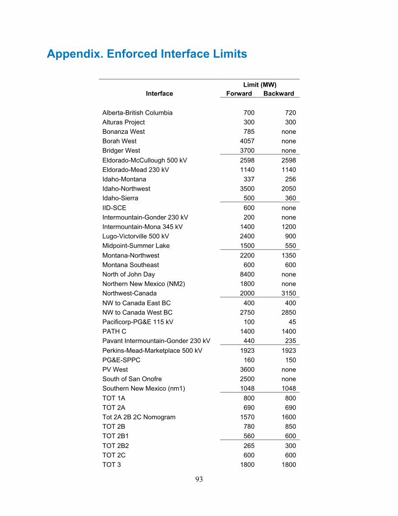
93
Appendix. Enforced Interface Limits
Interface Limit (MW)
Forward Backward Alberta-British Columbia 700 720 Alturas Project 300 300 Bonanza West 785 none Borah West 4057 none Bridger West 3700 none Eldorado-McCullough 500 kV 2598 2598 Eldorado-Mead 230 kV 1140 1140 Idaho-Montana 337 256 Idaho-Northwest 3500 2050 Idaho-Sierra 500 360 IID-SCE 600 none Intermountain-Gonder 230 kV 200 none Intermountain-Mona 345 kV 1400 1200 Lugo-Victorville 500 kV 2400 900 Midpoint-Summer Lake 1500 550 Montana-Northwest 2200 1350 Montana Southeast 600 600 North of John Day 8400 none Northern New Mexico (NM2) 1800 none Northwest-Canada 2000 3150 NW to Canada East BC 400 400 NW to Canada West BC 2750 2850 Pacificorp-PG&E 115 kV 100 45 PATH C 1400 1400 Pavant Intermountain-Gonder 230 kV 440 235 Perkins-Mead-Marketplace 500 kV 1923 1923 PG&E-SPPC 160 150 PV West 3600 none South of San Onofre 2500 none Southern New Mexico (nm1) 1048 1048 TOT 1A 800 800 TOT 2A 690 690 Tot 2A 2B 2C Nomogram 1570 1600 TOT 2B 780 850 TOT 2B1 560 600 TOT 2B2 265 300 TOT 2C 600 600 TOT 3 1800 1800

94
Interface Limit (MW)
Forward Backward TOT 4A 810 810 TOT 4B 680 680 TOT 5 1675 1675 West of Cascades-North 10200 none West of Cascades-South 7700 none Wyoming-Utah 1700 none Z1-Hassayampa-N. Gila 1905 none Z1-Palo Verde to Devers 2338 none Z2-SDGE Import Limit 4000 none Z2-SCIT 17700 17700 Z2-WOR 11823 none Z4-Moenkopi-El Dorado 1900 1645 Z4-Navajo-Crystal 1900 1900 Z4-Perkins-Mead 1238 1238 Z6-Path 26 4000 3000 Z7-Miguel-Tijuana 912 912 Z7-Imperial Valley-La Rosita 797 797 Z7-Path 45 408 800 Z9-HA-Red Butte PS 300 300 Z9-Pinto-4 Corners PS 600 600 Z9-Shiprock-Lost Canyon PS 400 400 Z9-Sigurd-Glen Canyon PS 300 300 Alberta-Saskatchewan 150 150 Brownlee East 1850 none California ISO-Mexico (CFE) 408 408 Cascade Crossing 2000 2000 Centennial 3000 none Cholla-Pinnacle Peak 1200 none COI 4800 3675 Combined 4a 4b 1096 none Coronado-Silver King-Kyrene 1600 none Coronado West 1494 1364 Crystal-Allen 950 950 Eagle Mtn 230 161 kV-Blythe 16 kV 72 218 East of Colorado River (EOR) 9300 none Four Corners 345 kV/500 kV 1000 1000 Inyo-Control 115 kV Tie 56 56 IPP DC Line 2400 1400 Midway-Los Banos 5400 3265 Montana Alberta Tie Line 325 300 North of Hanford 4100 none North of San Onofre 2440 none

95
Interface Limit (MW)
Forward Backward Northern-Southern California 4000 3000 Pacific DC Intertie South 2780 3100 pacific DC Intertie 3100 2780 SDG&E-Mexico (CFE) 408 800 Silver Peak-Control 55 kV 17 17 South of Alston 4100 none Southern CA Imports 14750 none Southern Navajo 3200 none Southwest of Four Corners 2325 none Sunrise Powerlink 1000 none TOT 7 890 none WALC Blythe-SCE Blythe 161 kV 218 218 West of Broadview 2573 none West of Colorado River (WOR) 10623 none West of Colstrip 2598 none West of Crossover 2598 none West of Hatwai 4277 none West of John Day 3450 none West of McNary 4500 none West of Slatt 5500 none WOR-n-El Dorado to Lugo 2754 none WOR-n-McCullough to Victorville 2592 none Z1-N. Gila-Imperial Valley 1905 none Z1-Imperial Valley to Miguel 2200 none Z1-Miguel Bank No. 1 1120 1120 Z1-Miguel Bank No. 2 1120 1120 Z1-North of Miguel 2000 none Z2: South of Lugo 6100 6100 Z3-Eldorado-Lugo 1645 1645 Z3-Market Place-Adelanto 1636 1636 Z3-Mccullough-Victorville 1385 1385 Z3-Mohave-Lugo 1386 1386 Z4-Jojoba-Kyrene 1732 1732 Z4-Peacock-Mead 508 508 Z5-Navajo-Moenkopi 1411 none Z5-South of Navajo 2264 none Z6-East of PV 8010 8010 Z8-Crystal-H Allen 500 kV PS 1300 none Z8-Crystal-H Allen 230 kV PS 950 None