quality loss function and tolerance design - nutek …nutek-us.com/qitt02 - taguchi loss function...

Quality Loss Function and Tolerance Design

A method to quantify savings from improved product and process designs


Nutek, Inc. All Rights Reserved Quality Loss Function and Tolerance Design www.Nutek-us.com Version: 8.1

2

Overview Attempts to define quality have demystified quality experts of all times. While many have forwarded numerous interpretations of quality is all about, Dr. Genichi Taguchi of Japan has proposed an intriguing definition of quality that covers a broader aspects than others. Dr. Taguchi defined quality as the ill effects (loss to the society) of un-quality of products and services the entire life of service in the hands of consumers. He further offered a mathematical formulation to quantify the magnitude of such effects, which he calls loss to the society, in terms of monetary units. Today, for all activities engaged in quality improvement of products and processes, the proposed concept of Loss Function is used mainly in the following tow ways:

- Quantify and compare merits of design improvements in terms of monetary values.

- Fine tune designs (Tolerance Design) based on optimum conditions obtained by Parameter Design.

Introduction

Evaluating and establishing improvements we achieve in performance, cost or quality is common tasks we perform at end of a project completion. Generally, we also express such improvements achieved in terms of percentage of the current level of performance. However, when asked to quantify the same improvement in terms of dollars we seem to have difficult time. Fortunately, the Loss Function formulation proposed by Dr. Genechi Taguchi allows us to translate the expected performance improvement in terms of savings expressed in dollars. Using the Loss Function concept, the expected savings from the improvement in quality, i.e., reduced variation in performance around the target can be easily transformed into cost. This session will present a quick review of the product and process design improvement using the Taguchi design of experiment (DOE) and discuss how the Loss Function is used to convert the improved performance in to expected dollar saving. Basic theories are covered and application demonstrated through examples. You would benefit most from this sessions if you have working knowledge of the DOE/Taguchi approach and wish to express improvements in terms of dollars.



3

TOPICS OF DISCUSSIONS 1. INTRODUCTION - Concepts - Math model - Purpose and application areas 2. EVALUATION OF $ LOSS - With target value - General quality characteristics - When other distribution parameters are known 3. COMPUTATION OF SAVINGS FROM CHANGES IN - S/N ratio - Mean Squared Deviation (MSD) - Std. Deviation and Average Value 4. RELATIONSHIPS BETWEEN LOSS AND PROCESS CAPABILITY (cpk) 5. GENERAL APPLICATION EXAMPLES 6. APPLICATION TO ACTUAL PROJECTS



4

SYMBOLS AND ABBREVIATIONS Y = Measured value of quality characteristic (QC) Ya = Average value of measured quality characteristic Yo = Target value of quality characteristic Tol = Tolerance of Y (in case of Nominal the best) Tc = Consumer Tolerance (in case of Bigger and Smaller characteristics) Ymin = Minimum value of Y Ymax = Maximum value of Y UCL = Upper control limit LCL = Lower control limit SDc = Standard déviation (conventional definition) SDT = Standard deviation (used in Taguchi method) MSD = Mean squared deviation S/N = Signal to ratio of measured data (QC) Cpk = Performance index L = Loss in terms of dollars Lc = Consumer Loss (cost of rejects when part is out of tolerance) K = A constant dependent on production parameters SQRT = Square root of the quantity within {}



5

1.0 INTRODUCTION Loss = $ value of a nonfunctioning single part (cost of rejects, rework, warranty, etc.) How to calculate loss? Conventional practice: Consider a BEARING HOUSING (Part)

Process Machine bearing seat to 2 +/- .003” Cost of machining each piece = $ 18.00/part Part dimension (Y) Loss (L) 2.0001 0 2.0015 0 1.998 0 2.004 $18.00 1.999 0 1.996 $18.00

2 +/- 0.003

FIG. 1 Bearing Housing

FIG. 2 Tolerance Limits

2 +/- 0.003

FIG. 3 Loss with Specification Limits

Y

Loss = $/Part

$18



6

KEY OBSERVATIONS Conventional practice: 1. If all parts are made within specification limits (SL), say at 2.001, theoretically, no part is wasted and thus no loss. 2. If all parts are made at or outside the SL, the entire cost of making a part is attributed to loss. Note: From no loss at just before 2.003 to $18 loss at just over 2.003 produces the step jump in loss (see FIG. 3) Taguchi Approach (Loss Function) There is loss even if the part is made within the SL. In other words there is loss as long as the part deviates from the target. (There is a warranty cost even if all parts are made to specification. Why?) Now let’s compare the two schools of thought.

Conventional Approach LOSS NO LOSS NO LOSS LOSS

LCL Target UCL FIG.4 Loss Zones with Specification Limits

Taguchi Approach LOSS Target UCL

FIG. 5 Loss zone with Taguchi Approach

Note: Loss at Y = Yo =/- Tol (At UCL) is same for both.



7

Basis for mathematical formulation - Assumption: Loss is continuous from target to UCL or LCL. It can be linear, quadratic or higher order. Taguchi formulated something that’s not relatively simpler yet worked well. His choice to express loss as L = K (Y - Yo)

2 where K is a constant Consider the case of Bearing housing machining process Yo = 2.000, Tol = .003 Cost of rejection, i.e., Loss when Y = UCL or LCL = $18.00 Since UCL = Yo + Tol Therefore L = K (Yo + Tol - Yo)

2 at point A or 18 = K(.003)2 or K = 2.00 x 106 $/sq. in or L = 2.00 x 106 (Y - Yo)

2 Thus when Y = 2.002 L = $2.00 and for Y = 2.003 L = $ 18.00

$18 LOSS NO LOSS NO LOSS LOSS

$ 2.00

LCL Target UCL FIG . 6 Loss Function



8

Examine how the loss formula works. L = K (Y - Y0)-

2 Assume Y = 5, tol = .02 Cost of reject = $6.00 Thus 6 = K (Yo +/- .02 - Yo)-

2 or K = 6/(.02 x .02) = 15,000 or L = 15,000 (Y - Y0)

2 Thus when Y = 5.005 L = 15,000 (5.005 - 5.00)2 = 0.375 etc. Y $ Loss 5.00 0 5.005 0.375 5.01 1.500 5.015 3.375 5.02 6.000

6. Loss (L) 4 2 0___________________________________________ 5.00 5.005 5.010 5.015 5.02 Measured QC, Y =>

FIG. 7 Loss with Positive Deviations



9

Terms and Units of Loss Parameters L + Loss is always expressed in terms of cost per unit of part Loss is same as cost of rejection when a part is made at UCL 0 < L < cost of rejection/making one part Y = Measured value of part QC, any defined units K = A constant. Unit is in $/Sq.in Tol = UCL or LCL - Yo

Yo = Target value of QC (in the same unit as Y) Total or average loss for a population of part: For a population of part produced at different dimensions, say, Y1, Y2, Y3, etc. average loss per product can be express as

( ) ( ) ( )[ ]L = K Y Y Y Y Y Y1 o 2 o n 0− + − + ⋅ ⋅ ⋅ ⋅ ⋅ + −2 2 2

/ N

or L = K (MSD) [by definition of MSD] Note: 1. L is always expressed as amount per part regardless of single or multiple unit of part information. If there is more than one part involved then instead of (Y - Yo)

2 MSD of the parts is used. 2. K = L/MSD or L/(Tol)2 implies that K should be found from either expression depending on the information available.

3. If tolerance is known then L = cost of rejection. When MSD is known loss needs to be computed from total cost of rejection and production rate.



10

Loss Function – Nominal the best This can be shown to be, MSD = σ 2 + ( Ya - Y0 )

2 Or

L = K (Y – Y 0)

2

0 Y0 Y0 - Tol Y0 + Tol

(Y1 – Y0)2

n 1 = + . . . + Σ

n

i = 1 MSD = (Y i – Y0)

2

(Y1 – Y0)2

(Yn – Y0)

2

K (Y – Y0)2 for one piece of data

L = K (MSD) for multiple (n) pieces of data

Where K = Lc / Tol2

Variability around average

L = K [σ 2 + ( Ya - Y0 )2 ]

Variability of the average from the target



11

Loss Function – Smaller is better This can be shown to be, MSD = σ 2 + Ya

2 Or

L = K Y 2

0

Y12

n 1 + . . . + Σ

n

i = 1 MSD = (Y i)

2

Y12

Yn

2

L = K [σ 2 + Ya2 ]

K (Y)2 for one piece of data L =

K (MSD) for multiple (n) pieces of data Where K = Lc / Tc

2



12

Loss Function – Bigger is better

Y0 Y0 - Tol Y0 + Tol

L = K [ 1/Y 2 ]

0

Y i2

1 Σ n

i = 1 MSD = n

1 =

Y12

1 Y3

2 1

Y22

1 Yn

2 1

+ + . . . +

K (1/Y)2 for one piece of data L =

K (MSD) for multiple (n) pieces of data Where K = Lc Tc

2



13

2.0 EVALUATION OF LOSS EXAMPLE 1 A machine makes 5000 parts at a cost of $3.00 each. Upon inspection 200 parts are rejected. Determine the loss per part. SOLUTION Total cost of rejection = 200 x $3.00 = $600 Average loss per part (L) = 600/5000 = $0.12/part (If all 500 parts were rejected, then loss (L) would become L = 3 x 5000/5000 = $ 3.00/part) EXAMPLE 2 A production process makes batteries for 9 +/- .25 volts applications at a cost of $0.75 each. Determine: a. Complete expression for loss function b. Loss when a part is made at 9.10 SOLUTION a) L = K (Y - Yo)

2 when Y = Y0 +/- .25 (at UCL or LCL) L = $.075 Thus .75 = K(.25)2 or K = .75/.0625 = 12 or L = 12 (Y - Y0 )

2 b) L = 12 (9.10 - 9.0)2 = $.12/part



14

EXAMPLE 3 A machine produces 10,000 6” long coil springs per day at a current production loss of $.30/part (overhead & rejection). Samples examined before and after improvement are as follows: Length BEFORE: 6.1 5.8 6.3 6.4 5.7 (5 examples) Length AFTER: 6.15 6.2 5.9 6.1 6.05 5.8 (6 examples) Calculate expected savings. SOLUTION BEFORE: MSD = [(6.2 - 6.0)2 + (5.8 - 6.0)2 + ....]/5 = .0772 S/N = - 10 log (.0772) = 11.12 L = K (MSD) or K = L/MSD = .30/.0772 = 3.886 or L = 3.886 (MSD) AFTER: MSD = [(6.15 - 6.0)2 + (5.8 - 6.0)2 + .....]/5 + .0772 S/N = 16.76 Since L = 3.886 (MSD) (constant K found earlier) L = 3.886 x .021 = $.08/part Therefore, Savings = (loss before - loss after)x monthly production = (.30 - .08) x 10,000 = $2,200/per month



15

EXAMPLE 4 A newly installed machine has the following performance characteristics: Part specifications: Y = 12 +/- .70, Cost per part = $1.50

production rate = 60,000 units/month Last month’s production: Std. Dev. = .25, Ya = 11.90 (10 samples) Current production: Std. Dev. = .21, Ya = 11.95 (12 samples) Determine saving expected. SOLUTION L = K (Y - Yo)

2 or 1.5 = K(O.70)2 or K = 1.5/(.70 x .70) = 3.06 Thus L = 3.06 x (Y - Yo)

2 also L = K (MSD) Last month: MSD = SDT

2 + M2 = SDc

2 x (N - 1)/N + M2 = (.25 x .25) (10 - 1)/10 + (12 - 11.9)2 = .066 Thus, loss L = 3.061 x (.066) = $0.20 Current condition: MSD = (.21 x .21) x (12 - 1)/12 + (.05 x .05) = .043 Thus, loss L = 3.061 x .043 = $0.13 Therefore, savings = (0.20 - 0.13) x 60,000 = $4,200/month



16

3.0 COMPUTATION OF SAVING FROM IMPROVEMENT IN S/N EXAMPLE 5 Old production status: Loss = $.20/part, MSD = .75 New production status: MSD = .50 Find $ savings as a percentage of loss in old production method. SOLUTION L = K ( MSD) Thus K = L/MSD = .20/.75 = 0.266 (from old production data) or L = 0.266 x (MSD) Loss in new production L = .266 x .50 = $ 0.133 % Savings = 100 x (Old loss - new loss)/old loss = 100 x (.20 - .133)/.20 = 33.5% EXAMPLE 6 A newly purchased milling machine was credited with improvement in S/N ratios of the machined parts from -18.5(before) to -12.5 (after). Determine the expected savings as a percentage of the loss before improvement. SOLUTION let SN2 = S/N (before) = -18.5 and SN1 = S/N (after) = -12.5 % Savings = [1 - 10-(SN2 - SN1)/10] x 100 = [1 - 10-(12.5 - (-18.5))/10] x 100 = [1 - 10-0.6] x 100 = [1 - .251] x 100 = 74.88%



17

4.0 RELATIONSHIPS BETWEEN LOSS AND PROCESS CAPABILITY INDEX CONTROL CHARACTERISTIC (Cpk)

( )

( )

C Y Y

3 x SD if Y Y

CY Y

3 x SD if Y Y

pk

a min

ca o

pk

max a

ca o

=−

<

=−

>

When Stand deviation is not known, but other production parameters are known, then Cpk can be calculated using the following relations M = Yo - Ya SDt = SQRT [(N -1)/N} x Sdc where SQRT = Square root {} MSD = Sdt

2 + M2 S/N = - 10 log (MSD) Loss L = K (MSD)

Ymin Ya Yo Ymax

FIG. 8 Cpk FORMULATION

X Cpk = X / (3 σ )



18

TABLE 1. RELATIONSHIPS AMONG COMMON PRODUCTION PA RAMETERS Assume that Yo = 40, Ymax = 45, Ymin = 35, N = 10 Cost of rejection = $2.50 and Loss constant K = 2.50/(5x5) = 0.10 For a given set of Ya and Sdc, all other parameters shown in the table can be calculated as shown below. Ya(1) SDc(2)_ Cpk(3)_ SDt(4) M(5) MSD(6) S/N(7) $L(8)

39 1.0 1.33 0.949 1.00 1.9006 -2.79 0.190

39 1.5 0.89 1.423 1.00 3.027 -4.81 0.300

39.5 1.0 1.50 0.949 0.50 1.151 -0.61 0.110

40.25 0.5 3.17 0.474 0.25 0.288 5.41 0.029

40 0.5 3.33 0.474 0.000 0.225 6.48 0.022

40 0.25 6.67 0.237 0.00 0.056 12.50 0.005

Sample calculation (first row of table 1) Given Ya = 39 and Sdc = 10 (3) Cpk = (39 -35)/(3x1) = 4/3 = 1.33 (4) SDT = SDcSQRT {9/10} = 0.949 (5) M + Yo - Ya = 40 - 39 = 1.0 (6) MSD = SDT

2 + M2 = (.949 x .949) + (1 x 1) = 1.900 (7) S/N = - 10 log (MSD) = -2.79 Using the value of loss constant, K, calculated above (8) L = K (MSD) = 0.10 x 1.900 (K = .10)



19 APPENDIX A DEVELOPMENT OF RELATIONSHIPS AMONG VARIOUS LOSS STATISTICS By definition Standard deviation SDc = ....(1) Mean Squared Deviation MSD = .... (2) In Taguchi approach, variation around the target is calculated as (Total sum of squares) ST = (Yi - Yo)

2 = = = = N x SDT

2 + N x M2

ST = N x (SDT2 + M2) .... (3)

where M = (Ya - Yo) N x SDT

2 = (Yi - Ya)2

that is SDT = .... (4) (Standard deviation as used in Taguchi approach which differs from the standard definition by a factor square root of. (N-1/N) Comparing the definitions of ST and MSD, ST = N x MSD ....... (5) therefore, MSD = SDT

2 + M2 ....... (6) 5.0 GENERAL APPLICATION EXAMPLES (Workout examples to facilitate application of certain formulae) 6.0 APPLICATION CASE STUDIES (Problems specific to the organization. Projects/data attendees bring to the class)



20 VII. EXERCISES (ON LOSS FUNCTION AND Cpk) For a machining operation the conditions presented as “GIVEN” are known. Calculate the quantities listed under “FIND”. The answers are as shown within ( ). Assume N = 24 if unspecified. 1. a) GIVEN: SDc = 2, N = 20 FIND: SDT = ? (1.924) b) GIVEN: SDc = 0.4, N = 12 FIND: SDT = ? (3.830) 2. a) GIVEN: SDT = 0.32, N = 8 FIND: SDc = ? (0.342) b) GIVEN: SDT = 6.0, N = 35 FIND: Sdc = ? (6.088) 3. a) GIVEN: MSD = 0.0025 FIND: S/N = ? (26.020) b) GIVEN: MSD = 135.5 FIND: S/N = ? (-21.32) c) GIVEN: MSD = 2.5 FIND: S/N = ? (-3.980) 4. a) GIVEN: S/N = -15.0 FIND: MSD = ? (32.6228) b) GIVEN: S/N = 0.50 FIND: MSD = ? (0.8913) c) GIVEN: S/N = 3.20 FIND: MSD = ? (0.4786) d) GIVEN: S/N = 12.5 FIND: MSD = ? (0.0562) 5. a) GIVEN: SDT = 2.5, FIND: MSD = ? (6.8125) M = 0.75 S/N = ? (-8.33) b) GIVEN: SDT = 0.03, FIND: MSD = ? (0.0011) M = 0.015 S/N = ? (29.49) 6. a) GIVEN: SDc = 95, FIND: MSD = ? (8561.9) M = 17 N = 12 S/N = ? (-39.33) b) GIVEN: SDc = 0.03, FIND: MSD = ? (0.0013) M = .02 N = 24 S/N = ? (28.29) 7. a) GIVEN: SDc = 0.5 LCL = 8 FIND: Cpk = ? (0.57) Yo = 9.00 Ya = 8.85 S/N = ? (6.06)



21 EXERCISE (Cont’d.) b) GIVEN: SDc = .03 UCL = 6.1 FIND: Cpk = ? (0.67) Yo = 9.00 Ya = 8.85 S/N = ? (6.06) c) GIVEN: SDc = 4.25 LCL = 6.1 FIND: Cpk = ? (1.65) Yo = 225 Ya = 221 S/N = ? (-15.09) d) GIVEN: SDc = 3.5 LCL = 200 FIND: Cpk = ? (2.00) Yo = 225 Ya = 221 S/N = ? (-14.32) e) GIVEN: SDc = 3.5 LCL = 200 FIND: Cpk = ? (2.29) Yo = 250 Ya = 226 S/N = ? (-10.80) 8. a) GIVEN: S/N = 8.75 UCL = 9.50 FIND: Cpk = ? (0.30) Yo = 9.0 Ya = 163 MSD = ? (0.1334) b) GIVEN: S/N = -12.5 UCL = 175 FIND: Cpk = ? (1.28) Yo = 160 Ya = 163 MSD = ? (17.783) 9. a) GIVEN: MSD = 3.2 UCL = 85 FIND: Cpk = ? (0.83) Yo = 80 Ya = 80.75 S/N = ? (-5.05) b) GIVEN: MSD = 1.3 UCL = 85 FIND: Cpk = ? (1.56) Yo = 80 Ya = 80.75 S/N = ? (-1.14) c) GIVEN: MSD = 3.2 UCL = 90 FIND: Cpk = ? (1.80) Yo = 80 Ya = 80.75 S/N = ? (-5.05) 10. a) GIVEN: S/N (before) = -13.2, S/N (after) = -8.75 FIND: Savings as a % of loss before experiment. (64.11%) b) GIVEN: S/N (before) = 5.5 S/N (after) = 8.9 FIND: Savings as a % of loss before experiment (54.29%) c) GIVEN: S/N (before) = -2.1 S/N (after) = 3.7 FIND: Savings as a % of loss before experiment (73.70%)



22

PRACTICE PROBLEMS (Loss Function Seminar)

1.1 A milling machine (M1) produces specimens whose surface finish readings (Bigger is better) are as follows: 8, 7, 8.5, 9.5, 9.3, 7.5, 8.6 (7 samples) Find: a) Average value [8.34] b) Standard Deviation [classical, .910] c) Standard Deviation - Taguchi form [.710] d) MSD [.0148] d) S/N [18.28] 1.2 The machine (M1) in problem 1.1 produces 1,500 parts per month at a cost of $175 per part. Historically 30 parts/month are returned by the assembly division which makes use of the part. Determine: a) Loss per part [$3.5] b) Monthly loss [$5250] c) Loss constant, K [Ans: 3.5 / 0.148 = 236.4, MSD = 0.0148] 1.3 To improve the milling process, the machine of problem 1.1 was equipped with a new tool holder at a cost of $3,500. The new process produced the following samples: 8.8, 9.5, 8.6, 8.9, 7.9, 9.2, 9.4 and 8.6 Determine: a) MSD [.01286] b) Loss at improved condition [L = K MSD =……. = $3.04/part] c) Monthly Loss [$4560] d) Monthly savings [$630] e) Effective annual savings [$630x12 - 3500 = $4060] 2.1 A manufacturer of a small servo motor spends $4,500 to reduce the operating noise of his product. The following noise reading (dB) were available from monthly production volume of 6,000 units. The total warranty and reject cost for the month $2500. Old Process: 75, 72, 67, 81, 80 and 74 New Process: 76, 66, 63, 58, 67, 56 and 60



23 Find: a) Loss before improvement [$.416/unit] b) MSD before [5622] c) Loss constant, K [7.4 x 10^-5] d) MSD after [4098] e) Loss after..[$.304/unit] f) Savings [$673] g) Return on investment (ROI) [$6.68 months] 2.2 Another sample taken from the improved process of problem 2.1 shows a S/N = -35.00. Using the same Loss constant, K = 7.4x10^-5, determine: a) Loss associated with this sample ($.234/part) b) If the cost to produce one motor is $25, what is the expected number of rejects out of monthly production of 6,000 units [56]. 3.1 A machine shop supplies castings for inner race of a certain roller bearing of size 12.50 +/- .200. The shop produces 15,000 units monthly at a total cost $45000. A sample part dimensions were as follows: 12.5, 12.4, 12.6, 12.55 and 12.7 Find: a) S/N [19.45] b) Loss constant [ 3/(0.2)^2 = 75] c) Loss [L = K MSD = 75 x 106-1.9 =$.851/unit] d) Loss per month [ 0.851 x 15000 = $12,769] e) Percent of part out of tolerance [28.36] 3.2 To improve the casting process of problem 3.1, the owner purchased a new molding equipment at a cost of $76,000. The new mold produced casting which shows S/N = 26.5. Determine: a) Loss [$.167] b) Monthly savings ($10,260) c) ROI [7.4 months] e) % of parts out of specs [5.56%]



24 3.3 A manufacturer of Tennis rackets intends to set 45 Lbs. tension in one of his product lines. The company spends $80,000 for total warranty (merchandise returned for out of specs tension). A sample data from monthly production of 35000 rackets show the following readings: 43, 48, 52, 44, 45, and 46 Lbs. To improve the product, the owner invested $250,000 in a new assembly operation which produced the following samples: 46, 43, 44, 45, 44, 44.5 and 45 Lbs. Determine: a) Loss constant [(80000/35000)/10.66) = .214] b) Loss from new production [ 0.214 x 1.03 = $.22/unit] c) New savings during the year. [(8000-7700) x 12 - 25000 = 614,500] 4.1 Cannons from three test tanks were shooting for a target 32,000 feet away. Determine the statistically superior performer by comparing their S/N (consider a sample of 10 shots for each). Cannon A: Cannon B: Cannon C: Average 32,200 feet 32,100 32,150 Std. Dev. 110 feet 200 120 FIND S/N Cannon A: Cannon B: Cannon C: Ans: [cannon C:S/n = -45, -45 > -46.89 > -47.17] 4.2 A pumpkin farmer finds his yield bringing the most returns when all pumpkins are of 20 Lbs. In the year 1989 his crop averaged 18 Lbs. with a Std. Deviation of 2.5 Lbs. His loss in that year due to unsold pumpkins was $2,400. The following year, the farmer employed a new agricultural method which improved yield to average 19 Lbs with Std. Deviation of 2.0. Determine the savings expected to result as a percent of loss in 1989. [Ans: 52.2%, 2,400 x 52.2 = $1,252.80]



25 5.1 A 25 cm gun barrel which bears a machining specification 25 +/- .250 costs $450 per piece to fabricate. Based on a sample of 20, the following statistics were computed: Average = 25.080 and Std. Dev. = .045 Determine: a) Cpk [1.26] b) Loss function [L = 7200 (y-25)2] c) Std. Dev.-Taguchi [.044] d) MSD [.044] e) S/N [20.788] f) Loss [$60/unit] ____________________________ _ _______________________________________ Answers:

(a) Cpk = (25.25 -25.080) /(3x o.o45) = 1.26 (b) K ==450 / (.250)^2 = 7200 (c) 0.045 (19/20)^.5 = 0.044 (d) (.044)^2 + (25.080 – 25 )^2 = 1.936 x 10^-3 + 6.4 x 10^-3 = 0.00834 (e) S/N = - 10 Log (0.00834) = 20.788 (f) L = K MSD = 7200 x 0.00834 = $ 60/unit



26

TOLERANCE DESIGN

by

Ranjit K. Roy, Ph.D.,P.E., PMP

Nutek, Inc. Bloomfield Hills, Michigan, USA.

E-mail: [email protected] Web Site: http://Nutek-us.com



27

Overview Tolerance Design is the third and final phases in the Taguchi quality improvement strategies. Starting with the System Design at the concept level that follows the Parameter Design, Tolerance Design is used to put the final touch by fin tuning the optimum factor selections identified in the previous phase. In Tolerance Design, the system is studied using current tolerances (factors at 2 or 3 levels) to determine which one to tighten and which one to be left alone. This is done by comparing the savings from quality improvement with the cost of upgrade. Approach Tolerance Design makes use of experimental designs with orthogonal arrays and the Taguchi Loss Function. The following are common steps in Tolerance Design. Step 1: Run experiments setting factors at current tolerance limits and perform ANOVA.

Step 2: Calculate loss for the current system performance [ L = K (MSD), or L = K VT , where VT = ST /(DOF)T ] Step 3: Determine potential savings (loss after – loss before) by adjusting factor levels:

• Calculate current loss using ANOVA (P%) • Estimate the new loss with upgraded factor level (better grade of

materials, part, etc.) Step 4: Calculate net gain (4) from savings from all factors at the improved condition.



28

Example: In a design for display control by a single-sided circuit board, the circuit output as potential difference between two critical points was measured as:

Y = Voltage as millivolt (mv)

The target voltage is 250 mv with +/- 20 mv. When the circuit is rejected due to performance outside the limits, the average rework costs is $42. The optimum nominal values of the factors determined from parameter design studies and the existing tolerances are as shown below. Figure T.1 Factors, Nominal Values and Tolerances Notation Factor Description Nominal Value Tolerance (σ) A Resistor – Left 40K Ohms 5% B Resistor - Right 120K Ohms 5% C Transistor 160 (hFE) 50 D Oscillator 555 5% E Jumper Pin 0.80 5%



29 The quality/grade of the parts under study can be upgraded to better quality (lower tolerances) with costs shown in the table below. Figure T.2 Upgrade Costs and Tolerances Type of Part Grades Cost Tolerance (σ) Resistor Low grade

High Grade Base Price 1.75

5% 1%

Transistor Low grade High Grade

Base Price 3.00

50 25

Oscillator Low grade High Grade

Base Price 1.90

5% 2%

Jumper Pin Low grade High Grade

Base Price 1.20

5% 1%

TOLERANCE DESIGN

Step 1: Run experiments setting factors at current tolerance limits and perform ANOVA.

To study the 5 factors, an experiment is designed using an L-8 array. The five factors A, B, C, D, and E each are assigned two levels of the factor as shown below: Level 1 = Nominal value – Tolerance (σ) Level 2 = Nominal value + Tolerance (σ)

Note: When a factor is assigned 3 levels, the nominal value makes one level and the other

two levels are assigned Nominal +/- 2/3 x Tolerance. Figure T.3 Factor Levels Studied



30

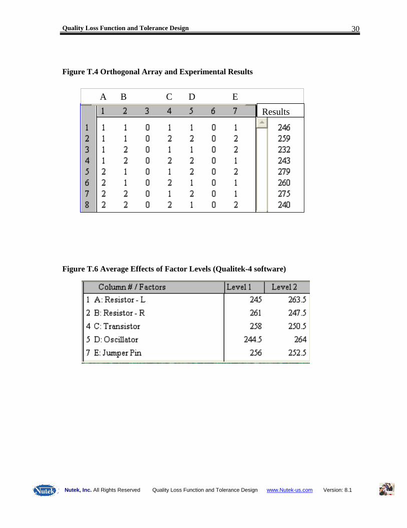
Figure T.4 Orthogonal Array and Experimental Results

Figure T.6 Average Effects of Factor Levels (Qualitek-4 software)

A B C D E

Results



31 ANOVA Calculations Correction Factor CF = ( 246 + 259 + 232 + 243 + 279 + 260 + 275 + 240)2/8

= 517,144 ST = 2462 + 2592 + 2322 + 2432 + 2792 + 2602 + 2752 + 2402 - CF = 519,136 - 517,144 = 1992 (Note that the hand calculations show difference in round-off from Qualitek-4 software out put shown in Fig. T.7) Since the Degrees of Freedom is 7, from Sums of Squares, ST, Variance can be calculated as: VT = 1992/ 7 = 284.6 Individual factor sums of squares can now be calculated for the significant factors as: (Factor average effects needed for factor sums of squares are shown in Fig. T.6) SA = 4 x (2452 + 263.52 ) - CF (4 results are used to calculate average effects) = 517,829 - 517,144 = 685 SB = 4 x (2612 + 247.52 ) - CF = 517,509 - 517,144 = 365 SC = 4 x (2582 + 250.52 ) - CF = 517,257 - 517,144 = 113 SD = 4 x (2442 + 2642 ) - CF = 517,905 - 517,144 = 761 SE = 4 x (2562 + 252.52 ) - CF = 517,169 - 517,144 = 25 (This factor is pooled or considered insignificant)



32 The error term is formed by pooling factor E and the effects from the two empty columns. Se = ST - ( Sum of squares of all significant factors, A, B, C & D) = 1992 – (685+365+113 + 761) = 1992 – 1924 = 68 The pooled degrees of freedom (DOF), fe becomes: fe = Total DOF – (DOF of all significant factors, A, B, C & D) = 7 – 4 = 3 Which gives the error variance, Ve, as: Ve = Se / fe = 68 /3 = 23 (approximately)

From the error sums of squares and DOF, the pure sum of squares, S’, for the factors can be calculated. SA

’ = SA - Ve x fA

= 685 – 23 x 1 = 662 which allows calculation of the relative contribution of factor A as: PA = SA

’ / ST

= 662/1992 = 33% Similarly, relative percent influence of all other factors is calculated as shown in the software output of ANOVA in Fig. T.7 and Fig. T.7a.

(PA = 33.2%, PB = 17.1%, PC = 4.4%, and PD = 37.0%)



33 Figure T.7 ANOVA

Figure T.7a Pie Chart Showing Relative Influence of Significant Factors



34

Step 2: Calculate loss for the current system performance The system response/output in this case, y = potential difference (mv), the tolerance, TOL = 20, and the average repair cost is $42 ( Lc). This specified values allows calculation of the loss constant, K, as: K = ( Lc)/(TOL)2

= 42/((20)2 = 0.105 [ L = K (MSD), or L = K VT , where VT = ST /(DOF)T ] Using the loss function in terms of variance, the current loss (from all factors/components) for the system now can be written as: L T(Current) = 0.105 x VT = 0.105 x 284.6 = 29.9 ($/Circuit board)

Step 3: Determine potential savings (loss after – loss before) by adjusting factor levels: • Calculate current loss using ANOVA (P%) • Estimate the new loss with upgraded factor level (better grade of

materials, part, etc.)

3a. Current loss from Factors Using ANOVA (P%) Since loss is proportional to the variance and since the relative percentage of factor influences (in right column in ANOVA) is based on the individual factor variances, the contribution to the total loss by individual factor can be calculated using the percentage of influence. LA = L T(Current) x PA = 29.9 x 33.2% = 29.9 x 0.332 = 9.93 ($/Circuit board)



35

LB = L T(Current) x PB = 29.9 x 17.1% = 29.9 x 0.171 = 5.11 ($/Circuit board)

LC = L T(Current) x PC = 29.9 x 4.4% = 29.9 x 0.044 = 1.32 ($/Circuit board)

LD = L T(Current) x PD = 29.9 x 37% = 29.9 x 0.37 = 11.06 ($/Circuit board) 3b. New Loss with Upgraded Parts The cost of upgraded parts and the new tolerances for each significant factor are shown in Fig. T.8 below. This data can be used to calculate the potential savings when parts of better grade are incorporated in the design. For example, when part is replaced by one with better grade at a cost of $1.75, the savings from such design can be calculated as: LA(New) = L A(Current) x (1% / 5% )2 (Loss is proportional to variance)

= 9.93 x 0.04 = 0.40 ($/Circuit board, loss is reduce from $9.93/board) Thus the quality improvement (QA) from part A in terms of dollars is: (QA)A = L A(Current) - LA(New) = 9.93 - 0.40 = $ 9.53 Of course, this improvement comes at cost of the upgraded part which for part A is $ 1.75. Thus, the net gain from selection of better grade part A is: (Net Gain)A = $ 9.53 - $1.75 = $7.78



36 Similarly, the net gain from all other parts can be calculated as shown below. (Net Gain)B = [L B(Current) - L B(Current) x (1% / 5% )2 ] - Upgrade Cost = [5.11 – 5.11 x 0.04] – 1.75 = [5.11 – 0.20] - 1.75 = $3.16 (Net Gain)C = [L C(Current) - L C(Current) x (25/ 50)2 ] - Upgrade Cost = [1.32 – 1.32 x 0.25] – 3.00 = [ 1.32 – 0.33] – 3.00 = - $2.01 (negative savings) Factor C has a negative savings which does not make it worthwhile to upgrade and will not be considered in the new design. (Net Gain)D = [L D(Current) - LD(Current) x (2% / 5% )2 ] - Upgrade Cost = [11.06 – 11.06 x 0.16] – 1.90 = [ 11.06 – 1.77] – 1.90 = $7.39 Figure T.8 Upgrade Costs and Tolerances for Significant Factors Type of Part Grades Cost Tolerance (σ) Resistor (A & B) Low grade

High Grade Base Price 1.75

5% 1%

Transistor (C) Low grade High Grade

Base Price 3.00

50 25

Oscillator (D) Low grade High Grade

Base Price 1.90

5% 2%

Step 4: Calculate net gain (4) from savings from all factors at the improved condition.

Based on the potential savings, only factors A, B, and D

Total Quality Improvement = 9.53 + 4.90 + 9.29 = 23.72 ($/Circuit board) Total Upgrade Cost (A, B, & D) = 1.75 + 1.75 + 1.90



37 = 5.40 ($/Circuit board) Total Net Gain = Total Improvement – Cost of Improvement = 23.72 - 5.40 = 18.32 ($/Circuit board) Figure T.9 Calculated Loss, Upgrade Cost and Net Gain Data Factor P% Loss -

current Loss – New $

Saving $

Upgrade Cost $

Net Gain $

Comment

A Resistor – L 33.2 9.93 0.40 9.53 1.75 7.78 Upgraded

B Resistor – R 17.1 5.11 0.20 4.90 1.75 3.16 Upgraded

C Transistor 4.4 1.32 0.33 0.99 3.00 -2.01 Not upgraded

D Oscillator 37 11.06 1.77 9.29 1.90 7.39 Upgraded

E Jumper Pin 0 0 -- -- 1.20 --

TOTAL 100 29.9 23.72 5.40 18.32 If the monthly production of this business unit is 4,500 Circuit boards per month (production volume), There will be potential to save 4,500 x $18.32 = $82,440 per month from this improvement obtained from TOLERANCE DESIGN study. Considerations for Applying Tolerance Designs for Your System

1. Completed optimizing your product or process using parameter design. 2. Identify a key response characteristic for which you know the TOLERANCE and

the LOSS sustained when performance is out of specification limits. 3. Identify factors to study for which there are better quality (grades) alternatives

available at a cost. 4. Have resources to carry out simpler experiments designed using orthogonal

arrays 5. Know how to perform ANOVA on results and be familiar with loss function.

quality loss function and tolerance design - nutek …nutek-us.com/qitt02 - taguchi loss function...

Documents