penalized nonparametric mean square estimation of the coefficients of diffusion processes

International Statistical Institute (ISI) and Bernoulli Society for MathematicalStatistics and Probability

Penalized Nonparametric Mean Square Estimation of the Coefficients of Diffusion ProcessesAuthor(s): Fabienne Comte, Valentine Genon-Catalot and Yves RozenholcSource: Bernoulli, Vol. 13, No. 2 (May, 2007), pp. 514-543Published by: International Statistical Institute (ISI) and Bernoulli Society for Mathematical Statisticsand ProbabilityStable URL: http://www.jstor.org/stable/25464888 .

Accessed: 24/06/2014 22:43

Your use of the JSTOR archive indicates your acceptance of the Terms & Conditions of Use, available at .http://www.jstor.org/page/info/about/policies/terms.jsp

.JSTOR is a not-for-profit service that helps scholars, researchers, and students discover, use, and build upon a wide range ofcontent in a trusted digital archive. We use information technology and tools to increase productivity and facilitate new formsof scholarship. For more information about JSTOR, please contact [email protected].

.

International Statistical Institute (ISI) and Bernoulli Society for Mathematical Statistics and Probability iscollaborating with JSTOR to digitize, preserve and extend access to Bernoulli.

http://www.jstor.org

This content downloaded from 185.2.32.106 on Tue, 24 Jun 2014 22:43:35 PMAll use subject to JSTOR Terms and Conditions

http://www.jstor.org/action/showPublisher?publisherCode=isibs

http://www.jstor.org/action/showPublisher?publisherCode=isibs

http://www.jstor.org/stable/25464888?origin=JSTOR-pdf

http://www.jstor.org/page/info/about/policies/terms.jsp


Bernoulli 13(2), 2007, 514-543 DOI: 10.3150/07-BEJ5173

Penalized nonparametric mean square estimation of the coefficients of

diffusion processes FABIENNE COMTE*, VALENTINE GENON-CATALOT** and YVES ROZENHOLC1

Laboratoire MAP5 (CNRS UMR 8145), UFR de Mathematiques et Informatique, Universite Paris 5 Rene

Descartes, 45 rue des Saints Peres, 75270 Paris Cedex 06, France.

E-mail: [email protected]; [email protected];

*yves. rozenholc @ math-info, univ-paris5.fr

We consider a one-dimensional diffusion process (Xt) which is observed at n + 1 discrete times with regular

sampling interval A. Assuming that (Xt) is strictly stationary, we propose nonparametric estimators of the

drift and diffusion coefficients obtained by a penalized least squares approach. Our estimators belong to a

finite-dimensional function space whose dimension is selected by a data-driven method. We provide non

asymptotic risk bounds for the estimators. When the sampling interval tends to zero while the number of

observations and the length of the observation time interval tend to infinity, we show that our estimators

reach the minimax optimal rates of convergence. Numerical results based on exact simulations of diffusion

processes are given for several examples of models and illustrate the qualities of our estimation algorithms.

Keywords: adaptive estimation; diffusion processes; discrete time observations; drift and diffusion

coefficients; mean square estimator; model selection; penalized contrast; retrospective simulation

1. Introduction

In this paper, we consider the following problem. Let (Xt)t>o be a one-dimensional diffusion

process with dynamics described by the stochastic differential equation:

dXt=b(Xt)dt+a(Xt)dWt, t > 0, X0 = n, (1)

where (Wt) is a standard Brownian motion and rj is a random variable independent of (Wt).

Assuming that the process is strictly stationary (and ergodic), and that a discrete observation

(XkA)\<k<n+\ of the sample path is available, we wish to construct nonparametric estimators of

the drift function b and the (square of the) diffusion coefficient a2. Our aim is twofold: to construct estimators that have optimal asymptotic properties and that

can be implemented through feasible algorithms. Our asymptotic framework is such that the

sampling interval A = An tends to zero while nAn tends to infinity as n tends to infinity. Nev

ertheless, the risk bounds obtained below are non-asymptotic in the sense that they are explicitly

given as functions of A or l/(nA) and fixed constants.

Nonparametric estimation of the coefficients of diffusion processes has been widely investi

gated in recent decades. The first estimators proposed and studied were based on a continuous

1350-7265 ? 2007ISI/BS



Penalized estimation of drift and diffusion 515

time observation of the sample path. Asymptotic results were given for ergodic models as the

length of the observation time interval tends to infinity: see, for instance, the reference paper by Banon [2], followed by more recent works by Prakasa Rao [30], Spokoiny [31], Kutoyants [28] orDalalyan[18].

Then discrete sampling of observations was considered, with different asymptotic frameworks, implying different statistical strategies. It is now classical to distinguish between low-frequency and high-frequency data. In the former case, observations are taken at regularly spaced instants with fixed sampling interval A and the asymptotic framework is that the number of obser vations tends to infinity. Only ergodic models are usually considered. Parametric estimation in this context was studied by Bibby and S0rensen [11], Kessler and S0rensen [27]; see also

Bibby et al. [12]. A nonparametric approach using spectral methods was investigated in Gobet et al. [24], where non-standard nonparametric rates were exhibited.

In high-frequency data, the sampling interval A = An between two successive observations is assumed to tend to zero as the number of observations n tends to infinity. Taking A? = l/n, so that the length of the observation time interval n An = 1 is fixed, can only lead to estimating the diffusion coefficient consistently. This was done by Hoffmann [25] who generalized results by Jacod [26], Florens-Zmirou [21] and Genon-Catalot et al. [22].

Now, estimating both drift and diffusion coefficients requires that the sampling interval An tends to zero while n An tends to infinity. For ergodic diffusion models, Hoffmann [25] proposes nonparametric estimators using projections on wavelet bases together with adaptive procedures. He exhibits minimax rates and shows that his estimators automatically reach these optimal rates

up to logarithmic factors. Hoffmann's estimators are based on computations of some random

times which make them difficult to implement. In this paper, we propose simple nonparametric estimators based on a penalized mean square

approach. The method is investigated in detail in Comte and Rozenholc [16,17] for regression models. We adapt it here to the case of discretized diffusion models. The estimators are chosen to

belong to finite-dimensional spaces that include trigonometric, wavelet-generated and piecewise polynomial spaces. The space dimension is chosen by a data-driven method using a penalization device. Due to the construction of our estimators, we measure the risk of an estimator f of f (with f = b,o-2)by E(||/-/||2), where ||/- /ll^^"1 ELi(A^a) ~/(^A))2. Wegive bounds for this risk (see Theorems 1 and 2). An examination of these bounds as A =

An ? 0

and nAn -> +oo shows that our estimators achieve the optimal nonparametric asymptotic rates

obtained in Hoffmann [25] without logarithmic loss (when the unknown functions belong to Besov balls). Then we proceed to numerical implementation on simulated data for several exam

ples of models. We emphasize that our simulation method for diffusion processes is not based on

approximations (like Euler schemes). Instead, we use the exact retrospective simulation method described in Beskos et al. [10] and Beskos and Roberts [9]. Then we apply the algorithms devel

oped in Comte and Rozenholc [16,17] for nonparametric estimation using piecewise polynomi als. The results are convincing even when some of the theoretical assumptions are not fulfilled.

The paper is organized as follows. In Section 2 we describe our framework (model, assump tions and spaces of approximation). Section 3 is devoted to drift estimation, and Section 4 to diffusion coefficient estimation. In Section 5 we study examples and present numerical simula tion results that illustrate the performance of estimators. Section 6 contains proofs. In Section 7 a technical lemma is proved.



516 F. Comte, V. Genon-Catalot and Y. Rozenholc

2. Framework and assumptions

2.L Model assumptions

Let (Xr)r>o be a solution of (1) and assume that n + 1 observations X*a, fc = 1,..., n + 1, with

sampling interval A are available. Throughout the paper, we assume that A = An tends to 0 and nAn tends to infinity as n tends to infinity. To simplify notation, we write A without the

subscript n. Nevertheless, when speaking of constants, we mean quantities that depend neither on n nor on A. We wish to estimate the drift function b and the diffusion coefficient o2 when X is stationary and geometrically /*-mixing. To this end, we consider the following assumptions:

Assumption 1.

(i) b e Cl(R) and there exists y>0 such thatjorall x e R, \b'(x)\ < y(l + \x\y). (ii) There exists bo such that, for all x, \b(x)\ < bo(l +1*|). (iii) There exist d > 0, r > 0 and R>0 such that, for all \x\ > R, sgn(jc)&(jt) < ?r \x\d.

Assumption 2.

(i) There exist crfi and a2 such that, for all x,0 < crfi <a2(x) <crf and there exists L such

that, for all (x, y) e R2, \a(x) -

a(y)\ < L\x -

y\1/2. (ii) a 6 C2(R) and there exists y > 0 such thatjorallx R, |o-'(jc)| + |o-"(x)| < y (1 +1*^).

Under Assumptions 1 and 2, equation (1) has a unique strong solution. Note that Assump tion 2(ii) is only used for the estimation of a2 and not for b. Elementary computations show that the scale density

s(x) = expj -2 / du \ [ Jo ?2(u) J satisfies f_OQs(x) dx = +oo =

f+0? s(x) dx, and the speed density m(x) = l/(a2(x)s(x)) satis

fies f- m(x) dx = M < +oo. Hence, model (1) admits a unique invariant probability tt(x) dx

with n(x) = M~lm(x). Now we assume the following:

Assumption 3. Xo = n has distribution ti .

Under the additional Assumption 3, (Xt) is strictly stationary and ergodic. Moreover, it follows from Proposition 1 in Pardoux and Veretennikov [29] that there exist constants K > 0, v > 0 and 0 > 0 such that

E(exp(v|X0|)) < +oo and Px(t)<KQ~0t, (2)

where Px(0 denotes the ̂-mixing coefficient of (Xt) and is given by

/+oo

7t(x)dx\\Pt(x,dx,)-7t(x,)dxf\\TV. -oo




The norm || ||tv is the total variation norm and Pt denotes the transition probability. In particular, Xo has moments of any (positive) order. Now, Assumption l(i) ensures that, for all t > 0, h > 0 and k > 1, there exists c ? c(k,y) such that

e( sup \b(Xs)-b(Xt)\k\T\<chk'2(l + \Xt\c), Vs [M+/*] /

where Tt = cr(Xs,s < t)\ for example, Gloter ([23], Proposition A). Thus, taking expectations, there exists c' such that

e( sup \b(Xs)-b(Xt)\k)<c'hk^2. (3)

The functions b and a2 are estimated only on a compact set A. For simplicity and without loss of generality, we assume from now on that

A = [0,1]. (4)

It follows from Assumptions 1, 2(i) and 3 that the stationary density n is bounded from below and above on any compact subset of R, and we denote by no, n\ two positive real numbers such that

0<7ro<7r(jc)<7ri VjcgA = [0, 1]. (5)

2.2. Spaces of approximation: piecewise polynomials

We aim to estimate the functions b and a2 of model (1) on [0,1] using a data-driven proce dure. For that purpose, we consider families of finite-dimensional linear subspaces of L2([0,1]) and compute for each space an associated least squares estimator. Then an adaptive procedure chooses among the resulting collection of estimators the 'best' one, in a sense that will be speci fied later, through a penalization device.

Several possible collections of spaces are available and discussed in Section 2.3. Now, to be

consistent with the algorithm implemented in Section 5, we focus on a specific collection, namely the collection of dyadic regular piecewise polynomial spaces, henceforth denoted by [DP]. We fix an integer r > 0. Let p > 0 also be an integer. On each subinterval Ij

= [(j ?

l)/2P, j/2P], j = 1,..., 2P, consider r + 1 polynomials of degree I, (fj,e(x), ? = 0,l,...,r, and set (pj,i(x)

= 0 outside Ij. The space Sm, m = (p,r), is defined as generated by the Dm = 2p(r + 1) functions (<Pj,e). A function t in Sm may be written as

IP r

j=\ t=0

The collection of spaces (Sm,m e Mn) is such that

Mn = {m

= (p, r), p e N, r {0, 1,..., rmax}, 2^(rmax + 1) < Nn}. (6)




In other words, Dm <Nn, where Nn <n. The maximal dimension Nn is subject to additional constraints given below. The role of Nn is to bound all dimensions Dm, even when m is random. In practice, it corresponds to the maximal number of coefficients to estimate. Thus it must not be too large. More concretely, consider the orthogonal collection in L2([?1,1]) of Legendre polynomials

(Qi,t > 0), where the degree of Qi is equal to ?, generating L2([?1,1]); see Abramowitz and Stegun ([1], page 774). These satisfy \Qe(x)\ < 1, for all x e [-1,1], Qi(l) = 1 and

f-i Qj(u)du = 2/(2i + 1). Then we set Pt(x) = (21 + l)^2Qe(2x

- 1) to obtain an ortho

normal basis of L2([0, 1]). Finally,

<pj,i(x) =

2P'2Pi(2px-j + l)tIj(x), j = l,...,2P,i = 0,l,...,r.

The space Sm has dimension Dm = 2p(r + 1), and its orthonormal basis described above satisfies

II 2P r II E1M* -Dm(r+1} - D^(rmax+1}

||y = l?=0 OO

Hence, for all t e 5W, ||f||oo < (rmax + l)1/2D^/2||r||, where ||f||2 = f^t2(x)dx, for t in

L2([0,1]), a property which is essential for the proofs.

2.3. Other spaces of approximation

From both theoretical and practical points of view, other spaces can be considered, such as

the trigonometric spaces [T], where Sm is generated by {1, 21/2cos(2ttjjc), 21/2sin(2ii7Jc) for

7 = 1,..., m], has dimension Dm = 2m + 1 and m e Mn = {1,..., [n/2] ?

1}; and the dyadic wavelet-generated spaces [W] with regularity r and compact support, as described, for example, in Daubechies [19], Donoho et al. [20] or Hoffmann [25].

The key properties that must be fulfilled to fit in our framework are the following:

(H\) Norm connection: (Sm)meMn *s a collection of finite-dimensional linear subspaces of

L2([0, 1]), with dimension dim(Sm) = Dm such that Dm < Nn < n, for all m e Mn, and satisfying:

There exists <f>o > 0 such that, for all m e Mn, for all t e Sm,

IUIIoo<*0?m/2|UI|.

An orthonormal basis of Sm is denoted by (^)xeAm? where |Am| = Dm. It follows from Birge and Massart [13] that property (7) in the context of (H\) is equivalent to:

There exists 4>0 > 0 such that ]P <p\ < ?oD - (8) IUeAm II oo

Thus, for the collection [DP], (8) holds with 4>q = rmax + 1. Moreover, for results concerning

adaptive estimators, we need an additional assumption:




(Hi) Nesting condition: (Sm)meMn *s a collection of models such that there exists a space denoted by Sn, belonging to the collection, with Sm c Sn for all m e Mn> We denote

by Nn the dimension of Sn: dim(<Sn) = Nn (Vm e Mn, Dm <Nn).

As far as possible below, we keep the notation general to allow extensions to spaces of approx imation other than [DP].

3. Drift estimation

3.1. Drift estimators: non-adaptive case

Let

YkA = xm-xkA and i

f{M)\(Xs)dWs (9) A A JkA The following standard regression-type decomposition holds:

1 H*+1)A YkA=b(XkA) + ZkA +

- / (b(Xs)-b(XkA))ds, A JkA

where b(XkA) is the main term, ZkA the noise term and the last term is a negligible residual.

Now, for Sm a space of the collection Mn and for t e Sm, we consider the following regression contrast:

1 n

Yn(t) = -Y[YkA-t(XkA)]2. (10)

The estimator belonging to Sm is defined as

bm= argrnin yn(t). (11) teSm

A minimizer of yn in Sm, bm always exists but may not be unique. Indeed, in some common situations the minimization of yn over Sm leads to an affine space of solutions. Consequently, it

becomes impossible to consider a classical L2-risk for the 'least squares estimator' of b in Sm. In contrast, the random W1 -vector (bm(XA),..., bm(XnA))' is always uniquely defined. Indeed, let us denote by nm the orthogonal projection (with respect to the inner product of W1) onto the

subspace {(t(XA),..., t(XnA))', t e Sm} of Rn. Then (bm(XA),..., bm(XnA))' = UmY, where Y = (YA,..., YnA)'. This is the reason why we define the risk of bm by

I n 1 E -Y{bm(XkA)-b(XkA)}2 =E(\\bm-b\\2n),

,ntx J where

1 n

H'Hn = -I>2^). (12) U

k=\




Thus, our risk is the expectation of an empirical norm. Note that, for a deterministic func tion t, E(||f ||2) = ||f||2 = ft2(x)dn(x) where n denotes the stationary law. In view of (5), the

L2-norm, || ||, and the L2(7r)-norm, || ||^, are equivalent for A-supported functions.

3.2. Risk of the non-adaptive drift estimator

Using (9), (10) and (12), we have

2 n

Yn(t) - Yn(b) = \\t - b\\2n + -

?> - t)(XkA)ZkA n

k=\

2 A r(*+DA + "7 I>

" ')(***) / (*<*') "

*(***))ds'

In view of this decomposition, we define the centred empirical process

1 n

Vn(t) = -Yt(XkA)ZkA. (13) nti

Now denote by bm the orthogonal projection of b onto Sm. By definition of bm, yn (bm) <yn (bm). So yn(bm)

- yn(b) < yn(bm)

- yn(b). This implies

\\bm -

b\\2n < \\bm

- b\\2n + 2vn(bm

- bm)

+ ? T(bm ~ bm)(XkA) / (b(Xs) - b(XkA))ds.

The functions bm and bm being A-supported, we can cancel the terms ||MAc||2 that appear in both sides of the inequality. This yields

\\bm -

btA\\2n < \\bm

- MA||2 + 2vn(bm

- bm)

+ ? T(bm - bm)(XkA) / (b(Xs) - b(XkA))ds. (14)

On the basis of this inequality, we obtain the following result.

Proposition 1. Let A = An be such that An -> 0, nAn/ln2(n) -> +oo when n -* +oo. Suppose that Assumptions 1, 2(i) and 3 hold and consider a space Sm in the collection [DP] with Nn =

o(nA/ln2(n)) (Nn is defined in (Hi))- Then the estimator bm ofb is such that

9 9 E(a2(X0))Dm , K" n\\bm-bA\\2n)<lJTx\\bm-bA\\2 + K I" m+rA + -, (15)

nA nA

where bA = btA and K, Kf and K" are positive constants.




As a consequence, it is natural to select the dimension Dm that leads to the best compromise between the squared bias term \\bm

- ^a II2 and the variance term of order Dm/(nA).

To compare the result of Proposition 1 with the optimal nonparametric rates exhibited by Hoffmann [25], let us assume that bA belongs to a ball of some Besov space, bA B<*,2,oo([0,1]), and that r -h 1 > a. Then, for ||*Alla,2,oo < L, we have \\bA

- bm\\2 < C(a, L)D~2xx. Thus,

choosing Dm = (nA)1^2""1"^, we obtain

E(||fcw - bA ||2) < C(a, L)(nA)-^^+l) + K'A + ^-. (16) nA

The first term (?A)_2a/(2a+1) is exactly the optimal nonparametric rate (see Hoffmann [25]). Moreover, under the standard condition A = o(l/(nA)), the last two terms in (15) are

0(l/(nA)), which is negligible with respect to (?A)_2a/(2a+1). Proposition 1 holds for the wavelet basis [W] under the same assumptions. For the trigono

metric basis [T], the additional constraint Nn < 0((nA)l^2/ln(n)) is necessary. Hence, when

working with these bases, if bA e Sa,2,oo([0,1]) as above, the optimal rate is reached for the same choice for Dm, under the additional constraint that a > 1/2 for [T]. It is worth stressing that a > 1/2 automatically holds under Assumption 1.

3.3. Adaptive drift estimator

As a second step, we must ensure an automatic selection of Dm, which does not use any knowl

edge of b, and in particular which does not require a to be known. The standard selection is

m = arg min [yn(bm) +pen(m)], (17) meMn

with pen(m) a penalty to be chosen appropriately. We denote by bm the resulting estimator and we need to determine pen(-) such that, ideally,

E(|fe-M2)<C inf (\\bA -bmf + E^XfDA +K'A + ̂, meMn\ nA / nA

with C a constant which should not be too large. We almost achieve this aim.

Theorem 1. Let A = An be such that An ?> 0, nAn/ln2(n) ? +oo when n -> +oo. Suppose

that Assumptions 1, 2(i) and 3 hold and consider the nested collection of models [DP] with maximal dimension Nn = o(n A/In2(n)). Let

pen(m)>Korf^, (18) nA

where k is a universal constant. Then the estimator b^ ofb with m defined in (17) is such that

mb*-bA\\l)<C inf (||^m-Z7A||2+pen(m)) + rA + ̂. (19) meMn nA




Some comments are in order. It is possible to choose pen(m) = KcrfDm/(nA), but this is not what is done in practice. It is better to calibrate additional terms. This is explained in Section 5.2. The constant k in the penalty is numerical and must be calibrated for the problem. Its value is

usually adapted by intensive simulation experiments. This point is also discussed in Section 5.2. From (15), one would expect to obtain E(a2(Xo)) instead of a2 in (18): we do not know if this is the consequence of technical problems or if it is a structural result. Another important point is that a2 is unknown. In practice, we just replace it by a rough estimator (see Section 5.2).

From (19), we deduce that the adaptive estimator automatically realizes the bias-variance

compromise: whenever bA belongs to some Besov ball (see (16)), if r + 1 > a and n A2 = o(l), bn\ achieves the optimal corresponding nonparametric rate, without logarithmic loss, contrary to Hoffmann's adaptive estimator (see Hoffmann [25], page 159, Theorem 5). As mentioned above, Theorem 1 holds for the basis [W] and, if Nn = o((nA)l/2/ln(n)), for [T] .

4. Adaptive estimation of the diffusion coefficient

4.1. Diffusion coefficient estimator: non-adaptive case

To estimate a2 on A = [0,1], we define

1 n

a2 = arg min yn(t) with yn(t) = - Y[UkA

- t(XkA)]2, (20)

teSm n f-f

and

Tj (*(*+i)A ~

xkA)2 n? UkA =-. (21)

A

For diffusion coefficient estimation under our asymptotic framework, it is now well known that rates of convergence are faster than for drift estimation. This is the reason why the regression

type equation has to be more precise than for b. Let us set

x/f = 2a'ob + \(o')2 + oo"\o2. (22)

Some computations using Ito's formula and Fubini's theorem lead to

UkA = a (XkA) + VkA + RkA

where VkA = V + V? + V , with

1 Tf /,(t+1)A l2 r(k+i)A -i

<=a[\L "a-)m-\-L ?Hx-n VkA = T / ((* + !>A - sy(Xs)o2(Xs)dWs, A JkA

V$=2b{XkA) tr(Xs)dWs, JkA




and

i / H*+l)A \ 2 2 / (*+!)* r(*+l)A RkA = -ll b(Xs)ds\ + - / (b(Xs)-b(XkA))ds

J cr(Xs)dWs

I H*+l)A + -

/ [(?+l)A-s]i/r(X,)ds.

Obviously, the main noise term in the above decomposition must be V^, as will be proved

below.

4.2. Risk of the non-adaptive estimator

As for the drift, we write

Yn(t) -

Yn(o2) = ||a2 -

11|2 + -

Y>2 -

t)(XkA)VkA + - T(a2

- t)(XkA)RkA.

n *-^ n *?" k=\ k=\

We denote by cr2 the orthogonal projection of a2 on Sm and define

1 n

Vn(t) = -Yt(XkA)VkA. ntx

Again we use the fact that yn(&2) ?

Yn(o2) < Yn(^m)

? Yn(o2) to obtain

2 n

\\a2m-o2t<\\o2m-a2t^2vn(d2m k=\

Analogously to what was done for the drift, we can cancel on both sides the common term

||a2lAc ||2. This yields

2 "

\\a2 -

a21|2 < ||a2 -

a21|2 + 2vn(&2 -

a2) + - ?>2

- *2)(XkA)RkA. (23) n

k=\

We obtain the following result.

Proposition 2. L^f A = An be such that An -> 0, nAn/ln2(n) -> +oo w/ze? n -> +oo. Suppose that Assumptions 1-3 fto/d and consider a model Sm in the collection [DP] with Nn = o(nA/ln2(n)), where Nn is defined in (H2). Then the estimator a2 of a2 defined by (20) is such that

^(H^m _

^A H?) ̂ 77rl ll^m ?

^A H + K-\~ K A -\-, (24) n n

where a\

= cr2tA, and K, K', K" are positive constants.




Let us make some comments on the rates of convergence. If o\ belongs to a ball of some

Besov space, say o\ e #a,2,oc([0,1]), and ||o^||a,2,oo < L> with r + 1 > a, then \\o\

- cr2 \\2 <

C(a, L)D-2a. Therefore, if we choose Dm = n^(7a+l\ we obtain

W* -

a21|2) < C(a, L)?"2a/(2a+1) + Kf A2 + ?. (25)

The first term n_2a/(2of+1) is the optimal nonparametric rate proved by Hoffmann [25]. Moreover, under the standard condition A2 = o(l/n), the last two terms are 0(1/n), that is, negligible with

respect to n~2a/(2of+1>.

4.3. Adaptive diffusion coefficient estimator

As previously, the second step is to ensure an automatic selection of Dm, which does not use any

knowledge on a2. This selection is done by

m = arg min [y?(a2) + pen(m)]. (26) meA4n

We denote by a? the resulting estimator and we need to determine the penalty pen as for b. For

simplicity, we use the same notation m in (26) as in (17) although they are different. We can

prove the following theorem.

Theorem 2. Let A = A? be such that An -> 0, ?An/ln2(n) ?> -hoo when n -> +oo. Suppose

that Assumptions 1-3 hold. Consider the nested collection of models [DP] with maximal dimen sion Nn < nA/ln2(n). Let

peh(m)>ic(j? ? , (27) n

where k is a universal constant. Then, the estimator <j? of a2 with m defined by (26) is such that

E(ll*| -

?\t) < C inf (Iki -

a\\\2 +pen(m)) + K'A2 + ?. (28) me/An n

As for the drift, it is possible to choose peii(m) = ko\Dm/n, but this is not what is done in

practice. Moreover, making such a choice, it follows from (28) that the adaptive estimator au

tomatically realizes the bias-variance compromise. Whenever a\ belongs to some Besov ball

(see (25)), if n A2 = o(l) and r -f 1 > a, a? achieves the optimal corresponding nonparametric rate n-2?/(2of+1)) without logarithmic loss, contrary to Hoffmann's adaptive estimator (see Hoff

mann [25], page 160, Theorem 6). As mentioned for b, Proposition 2 and Theorem 2 hold for the

basis [W] under the same assumptions on Nn. For [T], #? = o((n A)1 fl/ln(n)) is needed.




5. Examples and numerical simulation results

In this section, we consider examples of diffusions and implement the estimation algorithms on simulated data. To simulate sample paths of diffusion, we use the retrospective exact simulation

algorithms proposed by Beskos et al. [10] and Beskos and Roberts [9]. Contrary to the Euler

scheme, these algorithms produce exact simulation of diffusions under some assumptions on the drift and diffusion coefficient. Therefore, we choose our examples in order to meet these conditions in addition with our set of assumptions. For the sake of simplicity, we focus on models that can be simulated by the simplest algorithm of Beskos et al. [10], which is called EA1. More

precisely, consider a diffusion model given by the stochastic differential equation

dXt=b(Xt)dt + o(Xt)dWt. (29)

We assume that there is a C2 one-to-one mapping F on R such that %t = F(Xt) satisfies

dt=t=a(l=t)dt + dWt. (30)

To produce an exact realization of the random variable t=A, given that ?o = x, the exact algorithm EA1 requires that ofbeC1, and a2 + a' be bounded from below and above. Moreover, setting

A(?) = y a(u) du, the function

/*(?)= exp (A(?)-(?-*)2/2A) (31)

must be integrable on R, and an exact realization of a random variable with density proportional to h must be possible. Provided that the process (&) admits a stationary distribution that it may also be possible to simulate, using the Markov property, the algorithm can therefore produce an exact realization of a discrete sample (i-kA, k = 0,1,...,? + 1) in the stationary regime. We deduce an exact realization of (XkA

= F~l(i=kA), k = 0,..., n + 1).

In all examples, we estimate the drift function a(?) and the constant 1 for models like (30) or both the drift b(x) and the diffusion coefficient o2(x) for models like (29). Let us note that

Assumptions 1-3 are fulfilled for all the models (t-t) below. For the models (Xt), the ergodicity and the exponential /?-mixing property hold.

5.1. Examples of diffusions

5.1.1. Family 1

First, we consider (29) with

b(x) = -0x, a(jt) = c(l+jc2)1/2. (32)

Standard computations of the scale and speed densities show that the model is positive recurrent for 0 + c2/2 > 0. In this case, its stationary distribution has density

n(x) oc--.

(1+JC2)H4/c2



526 F Comte, V. Genon-Catalot and Y. Rozenholc

20i-1-1-1-1-1-1-1-1-1-1 14.-1-1-,-1-1-1-,-1-,

Y Drift U Volatility

15- - _12

data -true -estimate

10- 10

t* V ?'

~ -1 -0.8 -0.6 -0.4 -0.2 0 0.2 0.4 0.6 0.8 1 -1 -0.8 -0.6 -0.4 -0.2 0 0.2 0.4 0.6 0.8 1

Figure 1. dXt = -(0/c + c/2)tanh(cXr) + dWt, n = 5000, A =

1/20, 0 = 6, c = 2. Dotted line, true;

solid line, estimate. The algorithm selects (p, r) equal to (0, 1) for the drift, (0, 2) for a2.

If Xo = ^ has distribution 7r(jc)djc, then, setting v = 1 + 20/c2, v1/2 rj has Student distribution

t(v) which can be easily simulated. We now consider F\(x) =

f? l/(c(l + x2)l/2)dx = argsinh(jc)/c. By the Ito formula,

f, = F\(Xt) satisfies (30) with

a(?) = -(0/c + c/2) tanh(cf). (33)

Assumptions 1-3 hold for (?,) with ?o = F\(Xo). Moreover,

a2(^) + a\$) = {(0/c + c/2)2 + 0 + c2/2} tanh2(c?) - (0 + c2/2)

is bounded from below and above. And

A(f)= / Qf(w)dw = -(l/2-r-6>/c2)log(cosh(c^))<0,

so that exp(A(?)) < 1. Therefore, function (31) is integrable for all x and, by a simple rejection method, we can produce a realization of a random variable with density proportional to h(%) using a random variable with density M(x, A).




Note that model (29) satisfies Assumptions 1-3 except that a2(x) is not bounded from above.

Nevertheless, since Xt = F^~l(%t) = sinh(c?r), the process (Xt) is exponentially ^-mixing. The

upper bound o2 that appears explicitly in the penalty function must be replaced by an estimated

upper bound.

5.7.2. Family 2

For the second family of models, we start with an equation of type (30) where the drift is now

(see Barndorff-Nielsen [7])

?<? = -*(IT^-

(34)

The model for (?,) is positive recurrent on R for 0 > 0. Its stationary distribution is given by

;r(?) d? a exp(-2-^(l

+ c2i=2)l/A = exp(-2^)

expft>(?)),

where exp<p(?) < 1 so that a random variable with distribution 7r(?)d? can be simulated by simple rejection method using a double exponential variable with distribution proportional to

exp(?20|?|/c). The conditions required to perform an exact simulation of (%t) hold. More

I-.-1-,-i-,-1 100,-,-,-,-,-,-1

40 Yt Ut I data P

30- - .trUe -estimate .

20 t * t ,*'^.

70

*7 *** * it '"' 30- \ , - " '

-20- ' \ % ,

-3-2-10123 -3-2-10123

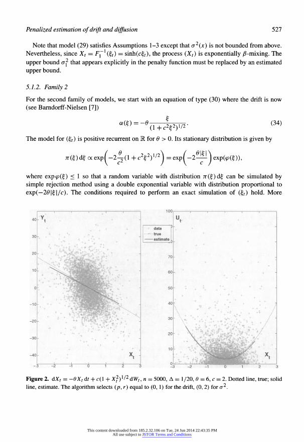
Figure 2. dXt = -0Xt dt + c(l + X2)1/2 dWt,n = 5000, A = 1/20, 6 = 6, c = 2. Dotted line, true; solid

line, estimate. The algorithm selects (p, r) equal to (0, 1) for the drift, (0, 2) for o2.



528 F Comte, V. Genon-Catalot and Y. Rozenholc

25 j-1-1-np-1-1-1-1-1 35 j-1-1-1-1-1-1-1-1 v Drift ii Volatility t ...w wt

20- . *

_30 - * , I data I 15" , ? * "

-true * C5 - *"" * ; ,*'* I-estimate!

10- " '

++--J&f?,'\t+ *< - 25~ * '

_15- * r "^ ~s - >"-v** :*'*-nL*v

Figure 3. dXr = -[0 + c2/(2cosh(X,))](sinh(X,)/cosh2(X,))df + (c/cosh(X,))dW,, n = 5000, A =

1/20, 0 = 3, c = 2. Dotted line, true; solid line, estimate. The algorithm selects (p, r) equal to (0,2) for the drift, (0,3) for a2.

precisely, a2 + a7 is bounded from below and above and A(?) = /0 o?(w)dw =

? (0/c2)(l +

c2^2)1/2. Hence exp(A(?)) < 1, (31) is integrable and we can produce a realization of a random variable with density proportional to (31). Lastly, Assumptions 1-3 also hold for this model.

We now consider Xt = F2(%t) = arg sinh(c?r), which satisfies a stochastic differential equation with coefficients

V 2cosh(x) / cosh2(jc) cosh(.x)

The process (X,) is exponentially ^-mixing as (?r). The diffusion coefficient a (x) is not bounded

from below but has an upper bound.

To obtain a different shape for the diffusion coefficient, showing two bumps, we consider

X, = G(&) = arg sinh(?, -

5) + arg sinh(?, + 5) where (fr) is as in (30)-(34). The function G(-) is invertible and its inverse has the explicit expression

G~\x) = -rp:-[49sinh2(jc) + 100 + cosh(*)(sinh2(jc)

- 100)11/2.

21/zsinh(x)L v /J




?i-r-1-1-1-1-1-1-1?I 7i?i-1-1-1-1-1-1-1-1?

Y U

10- ,. ? ""'/ . .*.,.. , -

_6- * -j data - '

.true .-*--*

* ,+.

. * -estimate

<- ̂'V\* f\ 5

'. /-"^ " "

V - 2_ ^ ' ' i

-4-3-2-1 0 1 2 3 4 ~-4 -3 -2 -1 0 12 3 4 -1-1-1-1-1-1-i-1-1 8(-1-1-i-1-i-1-1-1?

Y Drift U Volatility

10- / "

4 - 7

| data I ' t t . -true

6_ ^ \ x ~~ -estimate

*%Vjr* ~*** -"!* **' ^ * f *

'X - : *<W*+V- *^\ ,

' "^ ***'

* " <*" r"

-10 12 3 4 5 6 -10 12 3 4 5 6

Figure 4. Two paths for the two-bumps diffusion coefficient model Xt = G(i-t), d& =

-0&/(l + c2?2)1/2d/ + dWt, G(x) = argsinh(;c -

5) + argsinh(jc + 5), n = 5000, A = 1/20, 0 = 1, c = 10. Dotted line, true; solid line, estimate. The algorithm selects (p, r) equal to (0, 3) (above) and (2,0) (below) for the drift, (0, 6) (above) and (1,3) (below) for a2.




The diffusion coefficient of (Xt) is given by

a(x) = (l + (G-i(;c)-5)2)i/2

+ (l + (G-i(*) + 5)2)i/2-

(36)

The drift is given by b(x) = G'(G~l(x))a(G-l(x)) + \G"(G~l(x)).

5.2. Estimation algorithms and numerical results

We do not give here a complete Monte Carlo study but we illustrate how the algorithm works and what kind of estimate it delivers visually. We consider the regular collection [DP] (see Section 2.2). The algorithm minimizes the mean

square contrast and selects the space of approximation in the sense that it selects p and r for

integers p and r such that 2p(r + 1) < Nn < nA/ln2(n) and r e {0,1,..., /max)- Note that the

degree is global in the sense that it is the same on all the intervals of the subdivision. We take

''max = 9 in practice. Moreover, additive (but negligible) correcting terms are classically involved in the penalty (see Comte and Rozenholc [17]). Such terms avoid underpenalization and are in accordance with the fact that the theorems provide lower bounds for the penalty. The correcting terms are asymptotically negligible so they do not affect the rate of convergence. Thus, both

penalties contain additional logarithmic terms which have been calibrated in other contexts by intensive simulation experiments (see Comte and Rozenholc [16,17]).

The constant k in both penalties pen(ra) and peh(m) has been set equal to 4. We retain the idea that the adequate term in the penalty was E(a2(Xo))/A for b and

E(a4(Xo)) for a2, instead of those obtained (erf/A and o\, respectively). Indeed, in classi cal regression models, the corresponding coefficient is the variance of the noise. This variance

is usually unknown and replaced by a rough estimate. Therefore, in penalties, a2/ A and o\ are

replaced by empirical variances computed using initial estimators b, a2 chosen in the collection

and corresponding to a space with medium dimension: a2/A for pen(-) is replaced s2 = yn(b)

(see (10)); and o\ for the other penalty is replaced by s\ = Yn(o2) (see (20)).

Finally, for m = (p, r), the penalties pen(ra) for i = 1 and pen(ra) for / = 2 are given by

s2 4-i-2^(r + l+ln2-5(r + l)). n v

Figures 1-4 illustrate our simulation results. We have plotted the data points (XkA, YkA)

(see (9)) and (XkA, UkA) (see (21)), the true functions b and a2 and the estimated functions

based on 95% of data points. Parameters have been chosen in the admissible range of ergodicity. The sample size n = 5000 and the step size A = 1/20 are in accordance with the asymptotic context (large n and small A) and may be relevant for applications in finance. It is clear that the

estimated functions correspond very well to the true ones.

The simulation of sample paths does not rely on Euler schemes as in the estimation method.

Therefore, the data simulation method is disconnected with the estimation procedures and cannot

be suspected of being favourable to our estimation algorithm.




6. Proofs

6.1. Proof of Proposition 1

We recall that for A-supported functions, ||f ||2 = fA t2(x)n(x) dx. Starting from (13)?(14), we obtain

\\bm ~

bA\\2n < \\bm

- bA\\2n + 2\\bm

- bm\\x SUp |vn(0|

teSm,\\t\\?=l

1 JL f M*+i)A 1211/2 + 2\\bm-bm\\n

^lEW (b(Xs)-b(XkA))ds\

< \\bm-bA\\2n + \\\bm -bm\\l +8 SUP [vn(t)f

1 8 A/ /*^+1)A \2

Because the L2-norm, || ||^, and the empirical norm (12) are not equivalent, we must introduce a set on which they are and then prove that this set has small probability. Let us define (see (6))

^ = {^/|S--l <\yte (J (Sm + Sw0\{0}}. (37) 1 Mmi* Z m,m'eMn J

On Qn, \\bm -

bm\\2n < 2\\bm

- bm\\2n and \\bm

- bm\\2n

< 2(\\bm -

bA\\2n + \\bm -

bA\\2n). Hence, some elementary computations yield:

l-\\bm-bA\\2nt^n

7 8 n

/ r^+1)A \2 <Tll*m-*All2 + 8 SUp [Vn(t)]2 + ?-Y( / (b(Xs)-b(XkA))ds)

. 4 teSm,\\t\\n=l nAzf^\JkA J

Now, using (3), we obtain

' (MX,) -M^A))d5 < A / E[(b(Xs) -b(XkA))2]ds <cfA\ kA / JkA

Consequently,

E(||fem -Julian,) <7||^m -Z>A||2 + 32e( sup [vn(t)]2)+32cfA. (38) \t Sm,\\t\\n = \ /




Next, using (5), (7)-(9) and (13), it is easy to see that, since ||r||^ = 1 => \\t\\2 < 1 /no,

e( sup [vn(0]2) < ?e( sup [vn(t)]2) <?Y E[v2((px)]

WmJ>lbr=l / ^0 Wm,|l'll<l / n? teAm

I n

f /-(*+l)A l

K?1 AGAfli

<t>2Dm "

f / <*+?>* )

.?^,(fV(x,)J,).?fr'**?>>1'-,

Gathering bounds, and using the upper bound n\ defined in (5), we obtain

mbm-bA\\ltan)<l7i\\\bm-bA\\2 + 12 ? "" m +32c'A.

iron A

Now, all that remains is to deal with Qcn. Since \\bm ?

bA ||2 < \\bm ?

?||2, it is enough to check

that E(||?m ?

Z?||21qc) < c/n. Write the regression model as YkA = b(XkA) + ekA with

Â = - / [b(Xs)-b(XkA)]ds + - / a(Xs)dWs.

a Aa a jâ

Recall that Um denotes the orthogonal projection (with respect to the inner product of Rn) onto the subspace {(t(XA),..., t(XnA))f, t e Sm] of Rn. We have (bm(XA),...,bm(XnA))' =

TlmY, where Y = (YA,..., YnA)'. Using the same notation for the function t and the vector

(t(XA),..., t(XnA))', we see that

n

\\b - bm\\l = II* - nmb\\2n + ||nm^||2 < \\b\\2n 4-n"1 ?>2A.

i=\

Therefore,

1 n

E(||t - frmllôj) < E(||^||2^c) + -

?E(e2AlL^) k=\

< (El'2(b4(X0)) + E1/2(4))P1/2(^).

By Assumption l(ii) we have E(b4(X0)) < c(l + E(X$) = K. With the Burholder-Davis

Gundy inequality, we find




Under Assumptions 1,2(i) and 3 and inequality (3), we obtain E(e4A) <C(l +crf/A2) := C/ A2. The next lemma enables us to complete the proof.

Lemma 1. Let Qn be defined by (37) and assume that nAn/ln2(n) -> +oo when n - +oo.

Then, if Nn < O(nAn/In2(n)) for collections [DP] and [W], and if Nn < 0((nAn)l/2/ln(n)) for collection [T], then

P(??)<^. (39)

The proof of Lemma 1 is given in Section 7.

Now, we gather all terms and use (39) to obtain (15).

6.2. Proof of Theorem 1

The proof relies on the following Bernstein-type inequality:

Lemma 2. Under the assumptions of Theorem I, for any positive numbers and v, we have

p(X>(X*a)Z*a >n ,\\t\\2n < v2\

<expf-^A

Proof. We use the fact that J2k=\ t(XkA)ZkA can be written as a stochastic integral. Consider the process

n

Hnu = Hu =Y,tlkA,(k+i)A[(u)t(XkA)<j(Xu),

k=\

which satisfies #M2 <

af\\t ||^ for all u > 0. Then, writing Ms = f? Hu dWu, we obtain that

" f(k+l)A

A/(?+i)A = J]t(XkA) / <r(Xs)dWs, k=\ JkA

" f(k+l)A

(M)(n+l)A=J2t2(xkA) cr2(Xs)ds. *=1 Jk*

Moreover, (M)s = f? Hfdu < no2 A\\t\\l, for alls >0, so that (Ms) ande\p(kMs-X2{M)s/2)

are martingales with respect to the filtration Ts = cr(Xu,u < s). Therefore, for all s > 0, c> 0, d > 0, A > 0,

P(MS > c, (M)s <d)< PUxp(xMs - y (M)s\ > exp(xc

- ^-d\\

<exp(-(lc-^)).




Therefore,

F(MS > c, (M)s <d)< mf cxp(-(kc - jd\\

= expf-^-A

Finally,

P( ̂ 2t(XkA)ZkA >ne, \\t\\2n < v2\ =F(M(n+l)A>nAe, <M>(?+1)A < nv2a2A)

( (nAe)2 \ ( ne2A\

-exp(-w^j=exp("i^FJ Now we turn to the proof of Theorem 1. As in the proof of Proposition 1, we have to split

ll*m -

bA ||2 = ||&? -

bA \\ltQn + H^ -

bA \\2ntQcn. For the treatment of Qcn, the end of the proof of Proposition 1 can be used.

We now focus on what happens on Qn. From the definition of b^, we have, for all m e Mn,

Yn(bm) + pen(m) < yn(bm) + pen(m). We proceed as in the proof of Proposition 1 with the additional penalty terms (see (38)) and obtain

E(H6m -bA\\2ntnn) <77ri||Z>m -fcA||2+4pen(m) + 32E( sup [vn(t)l2t^n) \teSm+Sfi,\\t\\?=l /

-4E(pen(m)) + 32c'A.

The main problem here is to control the supremum of vn (t) on a random ball (which depends on

the random m). This is done by using the martingale property of vn(t). Let us introduce the notation

Gm(m')= sup |v?(f)|. teSm+Sm,,\\t\\n

= l

Now, we plug in a function p(m, m'), which will in turn fix the penalty:

G2m(m)lQn <[(G2m(m) -

p(m,m))tnn]+ + p(m,m)

^ J2 [{G2m(m')-p(m,m'))tQn]+ + p(m,m). m'eA4n

And pen is chosen such that Sp(m, m!) < pen(m) +pen(m'). More precisely, the next proposition determines the choice of p(m, m').

Proposition 3. Under the assumptions of Theorem 1, there exists a numerical constant k\ such

that, for p(m, m!) ? K\o\(Dm + Dm>)/(nA), we have

Q-Dmf

^[{G2m(m') -

p(m, m'))lQn]+ <

ca2-?^.




Proof of Proposition 3. The result of Proposition 3 follows from the inequality of Lemma 2 by the L2-chaining technique used in Baraud et al. [5] (see their Section 7, pages 44-47, Lemma 7.1, with s2 = a2/ A). D

It is easy to see that the result of Theorem 1 follows from Proposition 3 with pen(m) >

KG2Dm/(nA) and k = $k\.

6.3. Proof of Proposition 2

First, we prove that

EUE4Wa2 (40)

With the obvious convention, let RkA = R^ + R(^l + Rkl so that (40) holds if E[(R(^A)2] <

K[ A2 for i = 1,2,3. Using Assumption 1,

E[(Rkl)]?E{] b2(Xs)ds) <AEM b\Xs)ds\

< A2E(Z?4(X0))<cA2.

We also have

E[(Rkl)] < ^2 (E(/ (b(Xs)-b(XkA))ds\ EN cj(Xs)dWs) J

.

Using (3), we obtain

E[(/02]<c'A>. Lastly, using Assumptions 1 and 2 and equation (22),

e[(**a)2] ̂ XE(/A ((k+\)A-s)2^2(Xs)ds\ <E(*2(X0))^-<c"A2.

Therefore (40) is proved. We now return to (23) and recall that Qn is defined by (37). The treatment is similar to that for

the drift estimator. On S2?, ||ct2 -

al ||2 < 2||a2 - ^ fn,

\\ol-cr2A\\2n<\\a2-a2\\2n+l-\\a2-a2\\l+S sup v2(t) ?

teSm,Mx=l

8 "*=1




<ll^-^ll' + |ll^-^H'

+ 8 sup v2(0 + -^>2A.

Setting Bm(0,1) = {t e 5W, ||r|| < 1} and ?*(0,1) = {t e Sw, \\t\\? < 1}, the following holds on ?2n:

Tll*m-^ll5<Tlkm-^ll2+8 SUP v2?(t) +-f^R2^. 4 4 / ̂ S(Ofl) n^[

Moreover,

e( sup v2(t)) < ?e( sup v2(f))

< ? T E(v2(n)) V BS(0,1) / ^0 Wm(0,l) /

^0^

îEE(E^2(Â)v,2A) ^ XGAm \*=1 /

< _Q_J!L{12E(a4(Xo)) + 4ACM}, 7ron

where Cb,o = E((a'a2)2(Xo)) + crfE(b2(Xo)). Now using the condition on Nn, we have

ADm/n < ANn/n < A2/ln2(n). This yields the first three terms of the right-hand side of (24). The treatment of Qcn is the same as for b with the regression model UkA = cr2(XkA) + rjkA,

where nkA = VkA + RkA. By standard inequalities, E(n4A) < K{A4E(b*(X0)) + E(a8(X0))}.

Hence, E(Â) is bounded. Moreover, using Lemma 1, F(Qcn) < c/n2.

6.4. Proof of Theorem 2

This proof follows the same lines as the proof of Theorem 1. We start with a Bernstein-type inequality.

Lemma 3. Under the assumptions of Theorem 2,

nJ2t(XkAW^>ne, \\t\\2n < v2) <exp(-Cn 4 ff* 2 ) XJ~[ / V 2a^v2^ \\t\\00a(v/

and

p(^?'(**a)v*a >W(2^)1/2 +

or2||r||00x,||f||2<i;2J<exp(-Cnx). (41)

The non-trivial link between the above two inequalities is enhanced by Birge and Massart [14], so we just prove the first.




Proof of Lemma 3. First we note that

+00 p

E(eUf(x?A)V?<i>|jrnA) = i + J2 ̂ E{(t(XnA)V%y\FnA}

p=2P

+oo p

p=2P'

Next we apply successively the Holder inequality and the Burkholder-Davis-Gundy inequality with best constant (Proposition 4.2 of Barlow and Yor [6]). For a continuous martingale (Mt), with Mo = 0, for k > 2, M* = sup5<, \MS | satisfies ||M*\\k< ckll21| (M) xl2 \\k, with c a universal constant. And we obtain

2p~l \ /I /*(n+1)A 2p \ e(iv?(itiâ) < -^"iE(iy?A

a(xs)dws ^v

+ E(Jj

a2(X,)d5 J-?A)

< ^-(c2P(2p)PAP<T2p

+ AP<r2p) < (2axcfPpP.

Therefore,

OO p

E(e"'<x?A>V"A |THt) < 1 + V ^-(4ua2c2)P\t(XnA)\P.

k=2 F

Using pp/p\< qp~1, we find

oo

E(e"'^Â>"A) < 1 +e"! ?(4Ma2cV|*(X?A)|'

A:=2

_! (4Ma2c2e)2r2(XnA) <l+e -*-^ 1- (âêllrlloo)

Now, let us set

a = e(4ofc2)2 and b = 4a12c2e||r||00.

Since for x > 0, 1 + jc < e*, we obtain, for all u such that bu <l,

E(e*<*-^V.A) < 1 + aMV(X"A)<exPfat<2f2(X"A)). 1 - few \ 1 - bu )

This can also be written as

E(?p(?f(XBA)V?<i> -

a"XtoA))l^"A) " L




Therefore, iterating conditional expectations yields

E[e*p(?(?,<Xt4<>-2!^))]<K Then we deduce that

vHrt(Xki)V >ne,\\t\\2n<iA

< e- ce~**w-to)E ?p|?(?*<x4a)v?>

-

au2^Xbf)} < Q-nueQ(nau2v2)/(l-bu)

The inequality holds for any u such that bu < 1. In particular, w = e/(2av2 + eb) gives ?we +

av2u2/(l -

bu) = -(l/2)(e2/(2av2 + &) and therefore

P^(ftA)^>?, lk||2 <

^ <?p(-?^^). n

As for ̂^, we introduce the additional penalty terms and obtain that the risk satisfies

Wl -o-2A\\2ntnn) <lm\\ol -or2||2+4pen(m) + 32E( sup (vn(t))2tQf)

-4E(pen(m)) + K'A2, (42)

where Bnm m,(0,1) = {f Sm + Sm>, ||r|U = 1}. Let us denote by

Gm(m')= sup |i#>(01 > #* ,(0,1)

the main quantity to be studied, where

W(t)=l-?t(XkA)V%; n k=\




define also

k=\

As for the drift, we write

E(G2 (m)) < E[(G2 (m) - p(m, m))la?]+ + E(p(m, m))

< ? E[(G2n(/n,)-p(m,m,))ljJ?]++E(p(m,m)). m'eMn

Now we have the following statement.

Proposition 4. Under the assumptions of Theorem 2, for

, 4\Dm + Dm> , ?oYAn + An'Vl p(m,m)=K cr?\-+ ?^ -

I,

where /c* w a numerical constant, we have

E[(G2m(m') - p(m, m'))l^]+

< c?f?^

The result of Proposition 4 is obtained from inequality (41) of Lemma 3 by a L2(7r) ? L??

chaining technique. For a description of this method, in a more general setting, we refer to Propo sitions 2-4 in Comte ([15], page 282-287), to Theorem 5 in Birge and Massart [14] and to

Proposition 7 and Theorems 8 and 9 in Barron et al. [8]. Note that there is a difference be tween Propositions 3 and 4 which comes from the additional term ||f ||oo appearing in Lemma 3. For this reason, we need to use the fact that || ?A A/n ^Valloo/sup^^ \pk\ < || ? l^xllloo <

(^max + 1) An /n0 ^or (VOikeA an L2(7r)-orthonormal basis constructed by orthonormalisa tion of the ((p\). This explains the additional term appearing in p(m, m').

Choosing pen(ra) > ko\Dm/n with k = 16/c*, we deduce from (42), Proposition 4 and Dm <

Nn <nA/ln2(n) that

? A. 0 0 0 0 ~ _ A x-^ e~Dmf kof$& A2

+ 64E( sup (0<2)(O)2)+rA2 + E(||a|-or2||2lnc).

The bound for E(||ct? -

cr2||2lnc) is the same as that given in the end of the proof of Proposi tion 2. It is less than c/n provided that N? < ?A/ln2(?) for [DP] and [W] and N2 < ?A/ln2(?) for [T].




Since the spaces are all contained in a space denoted by Sn with dimension Nn bounded as

right above, we have

E( sup (v(2)(0)2)<-e( sup (vi2Ht))2)<KCb^2^<K'A2. KteB*^,!) / ^0 Ve<Sn,||f||=l / ^0"

The result of Theorem 2 follows.

7. Proof of Lemma 1

Using Baraud et al. [4], we prove that, for all n and A > 0,

P(fi?) < 2npx(qn A) + 2n2expf-C0 " Y (43)

V qnLn(<p)J

where Co is a constant depending on 7ro, 7ri, qn is an integer such that qn < n, and Ln(<p) is a

quantity depending on the basis of the largest nesting space Sn of the collection and is defined below. We recall that Nn = dim(<Sn).

We first prove (43). We use Berbee's coupling method as in Proposition 5.1 of Viennet [32] and its proof. We assume that n = 2pnqn. Then there exist random variables

X*A, / = 1,..., n,

satisfying the following properties:

For I = 1,..., pn, the random vectors U^\ = (X[2(?-iten+i]A. > x(2t-i)qnAY and

Ufa =

(X?2(^_i)^ +i]A' ' X%t-\)q a^

nave tne same distribution, and so have the vectors

Ui,2 =

(X[(2?-1)<7?+1]A, , X2tqttA)'

and Ufa

= (X*(2?_i)^ + i]A'

' X2lqn^'

. For ? = 1,..., pn, F(UiA # Ufa) < Px(qnA) and P(&,2 # Ufa)

< Px(qnA). For each 8 e {1,2}, the random vectors U* 8,..., U* 8 are independent.

Let us define Q* = {XiA = X*A, i = 1, ...,n). We have P(fl?) < P(^ H Q*) + P(?2*c) and

clearly

P(ft*c) < 2pnpx(qnA) < npx(qnA). (44)

Thus, (43) holds if we prove

P(?2? H S2*) < 2JV2expf-A0^- "

Y (45) "V 7tiqnLn((p)J

where Ln(0) is defined as follows. Let ((px)keAn be an L2(A, dx)-orthonormal basis of <S? and, as in Baraud et al. [4], define the matrices

y= ([ (pl(x)(pl(x)dx) 1 , B = (\\n<Py\\ooh^eAnxAn -\JA / Jk,XfeAnxAn

Then we set Ln(<f>) = max{p2(V), p(B)}, where, for any symmetric matrix M = (Mk,y),

p(M) = S*P[ak)tZkal<l Ex.A' \<*k\\<*k'\\Mw\.




We now prove (45). Let P*() := P(- n Q*). We use Baraud ([3], Claim 2 in Proposi tion 4.2). Consider vn(t) = (l/n)??=i['(*iA)

- E(f(X,A))], Bn(0,1) = {t e Sn, \\t\\n < 1}

and B(0, l) = {te Sn, \\t\\ < 1}. As, on A, n0 < n(x) < n\,

SUp \vn(t2)\= SUp Sf-1 <V SUp \vn(t2)\. t Bn(0,l) t Sn/{0} IIhItt teB(0,l)

Thus

P*( sup \vn(t2)\>po) <P*( sup \vn(t2)\>7t0po) \t Bn (0,1) / VeB(0,l) /

<P*( sup ^jT \aiay\\vn(<Pk<Pk')\>noPoY \ExeAnal^lk,kfeAn I

On the set {V(A, A/) e A2, \vn((pkcpk>)\ < 2Wkk>(2izxx)xl2 + 3B^x}, we have

sup J2 \"M\M<Px<Pk')\ < 2p(V)(27Tix)1/2 + 3/o(B)jc.

By choosing x = (po7To)2/(167riL?(</>)) and po = 1/2, and recall that 7To < n\, we obtain that

sup ^ \axax>\\vn((pk<Pk')\ < Po^o = ?. E^A,,^1 Xk'

This leads to

P*(??) = P*( sup \vn(t2)\>\) \teBn(0,\) l/

< P*({V(X, k') e A2, \vn((Pk(Pk>)\ > 2Vky(27Tlx)^2 + 3Bkk,x}).

The proof of (45) is then achieved by using the following claim, which is exactly Claim 6 in the

proof of Proposition 7 of Baraud et al. [4].

Claim 1. Let (<pk)keAn be an L2(A, djc) orthonormal basis of Sn. Then, for all x > 0 and all

integers q, 1 < q < n,

P*(3(A, X') e A2n/\vn(<pk<pk,)\ > 2VkX(2nlx)1'2 + 2^,^) <

2A^2exp^-?Y

Claim 1 implies that



542 F. Comte, V Genon-Catalot and Y. Rozenholc

and thus (45) holds true.

Again we refer to Baraud et al [4] (see Lemma 2 in Section 10). It is proved there that, for [T], Ln(4>) <

C^N2. For [W] and [DP] (see Sections 2.2 and 2.3 above), L?(0) < C'^Nn.

We now use (43) to complete the proof of Lemma 1. By assumption, the diffusion process X is

geometrically ^-mixing. So, for some constant 0, f$x(qnA) < e~ec*nA. Provided that A = An satisfies ln(n)/(n A) -> 0, it is possible to take qn = [5 ln(n)/(0 A)] + 1. This yields

The above constraint on A must be strengthened. Indeed, to ensure (39), we need

nA 61n2(n) ~ nA

Nn C0 hr(n)

for [W] and [DP]. This requires nA/ln2(n) ? +oo. The result for [T] follows analogously.

Acknowledgements

The authors wish to thank the Associate Editor and anonymous referees for comments that helped to significantly improve the paper.

References

[1] Abramowitz, M. and Stegun, LA. (eds) (1972). Handbook of Mathematical Functions with Formulas,

Graphs, and Mathematical Tables. New York: Wiley. MRO167642

[2] Banon, G. (1978). Nonparametric identification for diffusion processes. SI AM J. Control Optim. 16

380-395. MR0492159 [3] Baraud, Y. (2002). Model selection for regression on a random design. ESAIM Probab. Statist. 6 127

146.MR1918295

[4] Baraud, Y, Comte, F. and Viennet, G. (2001). Adaptive estimation in an autoregression and a geomet rical /J-mixing regression framework. Ann. Statist. 29 839-875. MR1865343

[5] Baraud, Y, Comte, F. and Viennet, G. (2001). Model selection for (auto)-regression with dependent data. ESAIM Probab. Statist. 5 33-49. MR1845321

[6] Barlow, M.T. and Yor, M. (1982). Semi-martingale inequalities via the Garsia-Rodemich-Rumsey lemma and applications to local times. J. Fund. Anal. 49 198-229. MR0680660

[7] Barndorff-Nielsen, O. (1978). Hyperbolic distributions and distributions on hyperbolae. Scand. J. Sta

tist. 5 151-157. MR0509451 [8] Barron, A.R., Birge, L. and Massart, P. (1999). Risk bounds for model selection via penalization.

Probab. Theory Related Fields 113 301-413. MR1679028

[9] Beskos, A. and Roberts, G.O. (2005). Exact simulation of diffusions. Ann. Appl. Probab. 15 2422

2444. MR2187299

[10] Beskos, A., Papaspiliopoulos, O. and Roberts, G.O. (2006). Retrospective exact simulation of diffu

sion sample paths with applications. Bernoulli 12 1077-1098. MR2274855




[11] Bibby, B.M. and S0rensen, M. (1995). Martingale estimation functions for discretely observed diffu

sion processes. Bernoulli 1 17-39. MR 1354454

[12] Bibby, B.M., Jacobsen, M. and S0rensen, M. (2002). Estimating functions for discretely sampled diffusion-type models. In Handbook of Financial Econometrics. Amsterdam: North-Holland.

[13] Birge, L. and Massart, P. (1997). From model selection to adaptive estimation. In D. Pllard,

E. Torgessen and G.L. Yang (eds), Festschrift for Lucien Le Cam: Research Papers in Probability and Statistics, pp. 55-87. New York: Springer-Verlag. MR1462939

[14] Birge, L. and Massart, P. (1998). Minimum contrast estimators on sieves: exponential bounds and

rates of convergence. Bernoulli 4 329-375. MR1653272

[15] Comte, F. (2001). Adaptive estimation of the spectrum of a stationary Gaussian sequence. Bernoulli 7

267-298. MR1828506

[16] Comte, F. and Rozenholc, Y. (2002). Adaptive estimation of mean and volatility functions in

(auto-Regressive models. Stochastic Process. Appl. 97 111-145. MR 1870963

[17] Comte, F. and Rozenholc, Y. (2004). A new algorithm for fixed design regression and denoising. Ann.

Inst. Statist. Math. 56 449-473. MR2095013

[ 18] Dalalyan, A. (2005). Sharp adaptive estimation of the drift function for ergodic diffusions. Ann. Statist.

33 2507-2528. MR2253093 [19] Daubechies, I. (1992). Ten lectures on wavelets. CBMS-NSF Regional Conference Series in ap

plied Mathematics, 61. Society for Industrial and Applied Mathematics (SIAM), Philadelphia, PA.

MR1162107 [20] Donoho, D.L., Johnstone, I.M., Kerkyacharian, G. and Picard, D. (1996). Density estimation by

wavelet thresholding. Ann. Statist. 24 508-539. MR1394974

[21] Florens-Zmirou, D. (1993). On estimating the diffusion coefficient from discrete observations. J. Appl. Probab. 30 790-804. MR1242012

[22] Genon-Catalot, V., Laredo, C. and Picard, D. (1992). Nonparametric estimation of the diffusion coef

ficient by wavelet methods. Scand. J. Statist. 19 319-335. MR1211787

[23] Gloter, A. (2000). Discrete sampling of an integrated diffusion process and parameter estimation of

the diffusion coefficient. ESAIM Probab. Statist. 4 205-227. MR1808927 [24] Gobet, E., Hoffmann, M. and Reiss, M. (2004). Nonparametric estimation of scalar diffusions based

on low frequency data. Ann. Statist. 32 2223-2253. MR2102509

[25] Hoffmann, M. (1999). Adaptive estimation in diffusion processes. Stochastic Process. Appl. 79 135

163. MR1670522 [26] Jacod, J. (2000). Non-parametric kernel estimation of the coefficient of a diffusion. Scand. J. Statist.

27 83-96. MR1774045 [27] Kessler, M. and S0rensen, M. (1999). Estimating equations based on eigenfunctions for a discretely

observed diffusion process. Bernoulli 5 299-314. MR1681700

[28] Kutoyants, YA. (2004). Statistical Inference for Ergodic Diffusion Processes. London: Springer

Verlag. MR2144185 [29] Pardoux, E. and Veretennikov, A.Yu. (2001). On the Poisson equation and diffusion approximation. I.

Ann. Probab. 29 1061-1085. MR1872736 [30] Prakasa Rao, B.L.S. (1999). Statistical Inference for Diffusion Type Processes. London: Edward

Arnold. MR1717690 [31] Spokoiny, V.G. (2000). Adaptive drift estimation for nonparametric diffusion model. Ann. Statist. 28

815-836. MR1792788 [32] Viennet, G. (1997). Inequalities for absolutely regular sequences: application to density estimation.

Probab. Theory Related Fields 107 467^92. MR1440142

Received December 2005 and revised October 2006



penalized nonparametric mean square estimation of the coefficients of diffusion processes

Documents