perceptual inference and information integration in brain and behavior pdp class jan 11, 2010

Perceptual Inference and Information Integration in Brain and Behavior

PDP ClassJan 11, 2010

How Neurons in Perceptual Systems Might Carry Out Perceptual ‘Inferences’

• Each neuron (or collection of neurons) is treated as standing for an hypothesis about what is out there in the world:– An oriented line segment at a particular point in space– Something moving in a certain direction– A monkey’s paw

• Note that a given object or scene might be characterized by a number of hypotheses; there might or might not be a separate ‘grandmother’ hypothesis.

• We treat the firing rate of each neuron as corresponding to the degree of belief in the hypothesis it participates in representing, given the available evidence, expressed mathematically as P(H|E)

• Question: How can we compute P(H|E)?

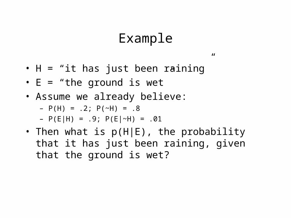
Example

• H = “it has just been raining”• E = “the ground is wet”• Assume we already believe:

– P(H) = .2; P(~H) = .8– P(E|H) = .9; P(E|~H) = .01

• Then what is p(H|E), the probability that it has just been raining, given that the ground is wet?

Theory of Perceptual Inference: How Can we Compute p(H|E)?

• Bayes’ Rule provides a formula:

P(H|E) = p(E|H)p(H) p(E|H)p(H) + p(E|~H)p(~H)where– P(H) is the prior probability of the hypothesis, H– P(E|H) is the probability of the evidence, given H– P(~H) is the prior probability that the hypothesis is false

(and is equal to (1-P(H))– P(E|~H) is the probability of the evidence, given that the

hypothesis is false.

• Bayes rule follows from the definition of conditional probability

Example

• H = “it has just been raining”• E = “the ground is wet”• Assume we believe:

– P(H) = .2; P(~H) = .8– P(E|H) = .9; P(E|~H) = .01

• Then what is p(H|E), the probability that it has just been raining, given that the ground is wet?

(.9*.2)/((.9*.2) + (.01*.8)) = (.18)/(.18+.008) = ~.96

• What happens if we change our beliefs about:– P(H)? P(E|H)? p(E|~H)?

How Should we Combine Two or More Sources of Evidence?

• Two different sources of evidence E1 and E2 are conditionally independent given the state of H, iff

p(E1&E2|H) = p(E1|H)p(E2|H) p(E1&E2|~H) = p(E1|~H)p(E2|~H)

• Suppose p(H), p(E1|H) and p(E1|~H) are as before andE2 = ‘The sky is blue’; p(E2|H) = .02; p(E2|~H) = .5

• Assuming conditional independence we can substitute into Bayes’ rule to determine that: p(H|E1&E2) = .9 x .02 x .2 = .47 .9 x .02 x .2 + .01 x .5 X .8

• In case of N sources of evidence, all conditionally independent under H, then we get:

p(E|H) = j p(Ej|H)

Conditional and Unconditional Independence

• Two variables (here, x and y) are ‘(unconditionally) independent’ iff p(x&y) = p(x)p(y) for all x,y.

• Two variables are ‘conditionally independent’ given a third (z) iff p(x&y|z) = p(x|z)p(y|z).

• The variables x and y are unconditionally independent in one of the graphs above. In the other graph, they are conditionally independent given the ‘category’ they are chosen from, where this is represented by the symbol used on the data point, but they are not unconditionally independent.

How this relates to neurons

• It is common to consider a neuron to have an activation value corresponding to its instantaneous firing rate or p(spike) per unit time.

• The baseline firing rate of the neuron is thought to depend on a constant background input called its ‘bias’.

• When other neurons are active, their influences are combined with the bias to yield a quantity called the ‘net input’.

• The influence of a neuron j on another neuron i depends on the activation of j and the weight or strength of the connection to i from j.

• Note that connection weights can be positive (excitatory) or negative (inhibitory).

• These influences are summed to determine the net input to neuron i:

neti = biasi + jajwij

where aj is the activation of neuron j, and wij is the strength of the connection to unit i from unit j.

Neuron i

Input fromneuron j

wij

A Neuron’s Activation can Reflect P(H|E)

• The activation of neuron i given its net input neti is assumed to be given by:

ai = exp(neti) 1 + exp(neti)

• This function is called the ‘logistic function’.

• It is easy to show thatai = p(Hi|E) iffaj = 1 when Ej is present, or 0 when Ej is absent;wij = log(p(Ej|Hi)/p(Ej|~Hi);biasi = log(p(Hi)/p(~Hi))

• In short, idealized neurons using the logistic activation function can compute the probability of the hypothesis they stand for, given the evidence represented in their inputs, if their weights and biases have the appropriate values.

ai

neti

Accurately Coding Probability in a Short Interval of Time

• If p(spike per 10 msec) = p(H|E) then having a single neuron to represent a hypothesis would make it difficult to get a clear estimate of P(H|E) within, say, 100 msec.

• However, suppose many (say, 10,000) neurons each encode the same hypothesis, and suppose that they produce spikes independently of each other (but based on the same p(H|E)).

• Then the number of spikes summed over the population would provide a very close approximation of p(H|E) even in a brief interval such as 10 msec.

Information Integration in Human Perception: The McGurk Effect (McGurk & MacDonald, 1976,

Nature 264, 746-748)

• First listen to clip with your eyes closed.

• Then listen again with eyes open.

• What you see appears to influence what you hear.

• What your hear probably sounds like ‘ba’ by itself.

• What does it sound like when you watch the face?

• Most people hear ‘da’ or ‘tha’.

• McGurk effect movie from USC.

Application of the model to a McGurk

experiment

• Massaro et al (2001) performed an experiment in which subjects received auditory inputs ranging from a good “ba” sound to a good “da” sound and visual speech inputs ranging from a good “ba” to a good “da”.

• The results are consistent with the model we have been describing, with auditory and visual input treated as conditionally independent sources of evidence for the identity of the spoken syllable.

• Note that when the auditory input is at either extreme, the visual input has little or no effect.

• These are examples of ‘floor’ and ‘ceiling’ effects that are often found in experiments.

• The model explains why the effect of each variable is only found at moderate values of the other variable.

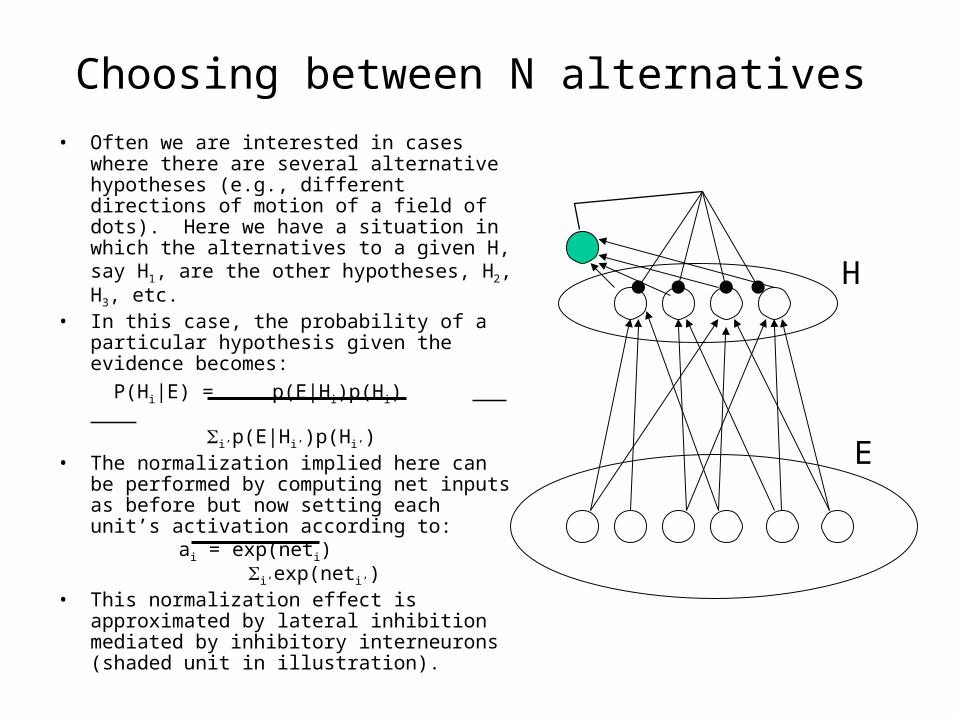
Choosing between N alternatives• Often we are interested in cases where

there are several alternative hypotheses (e.g., different directions of motion of a field of dots). Here we have a situation in which the alternatives to a given H, say H1, are the other hypotheses, H2, H3, etc.

• In this case, the probability of a particular hypothesis given the evidence becomes: P(Hi|E) = p(E|Hi)p(Hi) i’p(E|Hi’)p(Hi’)

• The normalization implied here can be performed by computing net inputs as before but now setting each unit’s activation according to:

ai = exp(neti) i’exp(neti’)

• This normalization effect is approximated by lateral inhibition mediated by inhibitory interneurons (shaded unit in illustration).

H

E

‘Cue’ Integrationin Monkeys

• Saltzman and Newsome (1994) combined two cues to theperception of motion:

– Partially coherent motion in a specific direction

– Direct electrical stimulation of neurons in area MT

• They measured the probability of choosing each direction with and without stimulation at different levels of coherence (next slide).

Model used by S&N:

• S&N applied a model that is structurally identical to the one we have been discussing:

– Pj = exp(yj)/i’exp(yj’)

– yj = bj + jzj + dx

– bj = bias for direction j

j = effect of micro-stimulation

– zi = 1 if stimulation was applied, 0 otherwise

d = support for j when motion is in that direction (d=1) or other more disparate directions (d=2,3,4,5)

– x = motion coherence

• Open circles above show effect of presenting visual stimulation in one direction (using an intermediate coherence) together with electrical stimulation favoring a direction 135° away from the visual stimulus.

• Dip between peaks rules out simple averaging of the directions cued by visual and electrical stimulation but is approximately consistent with the Bayesian model (filled circles).

perceptual inference and information integration in brain and behavior pdp class jan 11, 2010

Documents