performance analysis of a database layer’s migration …
TRANSCRIPT

PERFORMANCE ANALYSIS OF A DATABASELAYER’S MIGRATION FROM RDBMS TO A
NOSQL SOLUTION IN AMAZON AWS
MSc Thesis of Internet and Web Technology
written by
Carlo Butelli(born June 26st, 1984 in Grosseto, Italy)
under the supervision of Dhr. Dr. A.S.Z. Belloum, and submitted to theBoard of Examiners in partial fulfillment of the requirements for the degree of
MSc in Computer Science
at the Universiteit van Amsterdam and Vrije Universiteit Amsterdam.
Date of the public defense: Members of the Thesis Committee:Date of publication(soon) Dr. Adam S.Z. Belloum
Dr. Patricia Lago

This is the Dedication.

Declaration of originality
I hereby declare that this thesis was entirely my own work and that any addi-tional sources of information have been duly cited.
I certify that, to the best of my knowledge, my thesis does not infringe uponanyone’s copyright nor violate any proprietary rights and that any ideas, tech-niques, quotations, or any other material from the work of other people includedin my thesis, published or otherwise, are fully acknowledged in accordance withthe standard referencing practices. Furthermore, to the extent that I have in-cluded copyrighted material, I certify that I have obtained a written permissionfrom the copyright owner(s) to include such material(s) in my thesis and haveincluded copies of such copyright clearances to my appendix.
I declare that this thesis has not been submitted for a higher degree to anyother University or Institution.

Contents
1 Introduction 11.1 Scope of the Work . . . . . . . . . . . . . . . . . . . . . . . . . . 21.2 Research Questions . . . . . . . . . . . . . . . . . . . . . . . . . . 21.3 Structure of the report . . . . . . . . . . . . . . . . . . . . . . . . 31.4 Useful used tools . . . . . . . . . . . . . . . . . . . . . . . . . . . 3
2 Background and Literature Review 52.1 Related Work . . . . . . . . . . . . . . . . . . . . . . . . . . . . . 52.2 Overview of RDBMS . . . . . . . . . . . . . . . . . . . . . . . . . 6
2.2.1 The Relational model . . . . . . . . . . . . . . . . . . . . 82.2.2 The ACID properties . . . . . . . . . . . . . . . . . . . . . 102.2.3 SQL Language . . . . . . . . . . . . . . . . . . . . . . . . 112.2.4 Amazon RDS for MariaDB . . . . . . . . . . . . . . . . . 11
2.3 Sharding . . . . . . . . . . . . . . . . . . . . . . . . . . . . . . . . 122.4 Replication . . . . . . . . . . . . . . . . . . . . . . . . . . . . . . 132.5 Eventual & Strong consistency . . . . . . . . . . . . . . . . . . . 142.6 NoSQL Databases . . . . . . . . . . . . . . . . . . . . . . . . . . 14
2.6.1 NoSQL data models . . . . . . . . . . . . . . . . . . . . . 142.6.2 The CAP Theorem . . . . . . . . . . . . . . . . . . . . . . 172.6.3 Query language . . . . . . . . . . . . . . . . . . . . . . . . 182.6.4 Overview of Amazon DynamoDB . . . . . . . . . . . . . . 18
3 Framework design and DB engines 203.1 How do DBs store data? . . . . . . . . . . . . . . . . . . . . . . . 20
3.1.1 Amazon RDS for MariaDB . . . . . . . . . . . . . . . . . 203.1.2 Amazon DynamoDB . . . . . . . . . . . . . . . . . . . . . 22
3.2 Database manipulation . . . . . . . . . . . . . . . . . . . . . . . . 253.2.1 Insert operation . . . . . . . . . . . . . . . . . . . . . . . 253.2.2 Update operation . . . . . . . . . . . . . . . . . . . . . . . 283.2.3 Delete operation . . . . . . . . . . . . . . . . . . . . . . . 293.2.4 Read operation . . . . . . . . . . . . . . . . . . . . . . . . 31
3.3 Indexing . . . . . . . . . . . . . . . . . . . . . . . . . . . . . . . . 343.3.1 MariaDB . . . . . . . . . . . . . . . . . . . . . . . . . . . 353.3.2 DynamoDB . . . . . . . . . . . . . . . . . . . . . . . . . . 35
3

CONTENTS 4
3.4 Join operations . . . . . . . . . . . . . . . . . . . . . . . . . . . . 363.5 Highlights . . . . . . . . . . . . . . . . . . . . . . . . . . . . . . . 37
4 Benchmarking Framework Implementation 384.1 Caching . . . . . . . . . . . . . . . . . . . . . . . . . . . . . . . . 394.2 API level(Django Framework) . . . . . . . . . . . . . . . . . . . . 40
4.2.1 Operation’s definitions . . . . . . . . . . . . . . . . . . . . 404.2.2 Django models . . . . . . . . . . . . . . . . . . . . . . . . 414.2.3 Boto 3 SDK for DynamoDB . . . . . . . . . . . . . . . . . 444.2.4 Database Tables . . . . . . . . . . . . . . . . . . . . . . . 484.2.5 Indexes . . . . . . . . . . . . . . . . . . . . . . . . . . . . 494.2.6 Items’ types . . . . . . . . . . . . . . . . . . . . . . . . . . 49
4.3 DB Connection time, logic behind the schema . . . . . . . . . . . 504.3.1 Used queries . . . . . . . . . . . . . . . . . . . . . . . . . 524.3.2 TCP ping . . . . . . . . . . . . . . . . . . . . . . . . . . . 52
4.4 Benchmarking operators . . . . . . . . . . . . . . . . . . . . . . . 53
5 Discussion of analysis 555.1 Connection measurements . . . . . . . . . . . . . . . . . . . . . . 555.2 Key metrics . . . . . . . . . . . . . . . . . . . . . . . . . . . . . . 565.3 Speed and throughput . . . . . . . . . . . . . . . . . . . . . . . . 575.4 Scalability . . . . . . . . . . . . . . . . . . . . . . . . . . . . . . . 62
6 Conclusions and future work 636.1 Conclusions . . . . . . . . . . . . . . . . . . . . . . . . . . . . . . 636.2 Future work . . . . . . . . . . . . . . . . . . . . . . . . . . . . . . 65
A Standard Deviation on measurements 70
B Measurement Tables 71

CONTENTS 5
List of Abbreviations
DBMS DataBase Management System
NoSQL ”Not Only SQL”
RDBMS Relational Database Management System
SQL Structured Query Language
UML Unified Modeling Language
Abstract
Nowadays, IT is dealing with a huge constant increase of data that is comingfaster and in greater volumes than ever before. Companies are exploring waysto face the rise of these data and to create value out of them, being innovativeand gaining competitive advantages. Such data is commonly referred to as BigData and besides standard SQL databases, NoSQL databases have been createdto better deal with this situation.
Traditional SQL databases provide powerful mechanisms to store and querystructured data under strong consistency and transaction, guaranteeing dataintegrity and consistency. Nowadays, this kind of database turned out to becritical in managing the explosion of Big Data especially because they are notcompletely able to scale too big, too fast or with ”diverse” data. This can reflecttheir ”failure” to cope with high-volume, high-velocity, and high-variety of data.
This new technology called NoSQL database instead is gaining more andmore popularity with the debut of social media and cloud computing. NoSQLbasically deal with non-structured or semi-structured data and certain work-loads seems to scale better and to be more cost-effective using this solution.
The main goal of this research is to investigate on the performance ofthis NoSQL database compared with an instance of the already popular SQLdatabase underlying advantages and disadvantages by performing some bench-mark analysis. The entire research has been done under the profile of a companythat currently is intended to migrate the whole system to the cloud(AmazonAWS) and make use of the NoSQL Amazon DynamoDB for tables with highload of reads.

Chapter 1
Introduction
Nowadays, the huge growth in spread of mobile devices, social networks, “Inter-net scale” web applications and Web 2.0 are making the world more information-driven and companies have been starting to seek new ways to deal with the largeamount of data coming up time by time. One of the major goal for companiesis to get value out of those data, being innovative and gaining competitive ad-vantages in order to increase the speed up of getting and tracking data in theirown applications.
Today, software architects and developers have several choices for data stor-age and persistence. At the top of them there are two main technologies, thewell known RDBMS and the novel data storage system called NoSQL, mostcommonly referred to as ’Not Only SQL’.
RDBMS guarantees and have reached an unmatched level of reliability, sta-bility and support through decades of development. However, in recent years,the amount of useful data in some application areas has become so vast that itcannot be stored or processed by traditional database solutions.
Its structure presents some ”deficiency”. The information that are spread onseveral tables linked together through a clause called JOIN, eventually involvesmany query requests to the database producing high slowdowns. Moreover,those incoming requests are also outgoing, meaning that every simple insert,update or delete operation even involving a single record, it will entail a mixof requests to the database and joining several tables in a distributed system ispretty difficult end expensive.
On the other side, NoSQL is a term that describes a broad class of technolo-gies surged in popularity providing a different approach to data storage com-pared with traditional SQL databases. Some refer to them as ’No relational’or ’No RDBMS’, some others simple prefer to call them Distributed DatabaseManagement Systems. Among the main features they seem to be able to over-take some of the problems above by offering horizontal scalability, elasticity andhigher availability than relational databases by sacrificing querying capabilitiesand consistency guarantees. [13]
SQL in most typical situations scale vertically, which means that they can
1

CHAPTER 1. INTRODUCTION 2
face the increase of loads by increasing RAM and SSD capacities, CPU and soon, on a single server.
In a Web application where the number of users and data will start growingbeyond expectations making it hard to keep up with the data requirement, anRDBMS will start to feel the heat and a migration from a relational databaseto a non-relational one sometimes could be a powerful solution.
The popularity of NoSQL has some key factors as compared to the RDBMSsystems. Some of them are the increase of data availability, a lightweight com-puting (no more operations on data aggregation), more scalability(from verticalto horizontal just adding Servers) even if it could present some drawbacks likedata redundancy.
1.1 Scope of the Work
This thesis is aimed to independently investigate the performance of the NoSQLkey-value store Amazon DynamoDB against Amazon RDS for MariaDB as SQLdatabase in the provision of migrating the database layer from a RDBMS to aNoSQL solution. The comparison has been made through simple operations,that are, read, write, delete and update measuring their operational time tohave a good estimation to what extent migrating the database layer (or a partof it) to a new solution could worth. This crucial step has been done by takinginto consideration the literature review. An additional operation that iteratesthrough all keys has also been investigated. Experimental results measure thetiming of these operations and how the databases stuck up against each other.
1.2 Research Questions
RQ1 What are the main features of NoSQL databases and why companies aremore and more going to adopt such structure for their database layer?Which trade offs are involved in the choice of a NoSQL database?
RQ2 Considering the increase of data available in a fast growing company, towhat extent making use of a database layer based on NoSql instead of thetraditional RDBMS may be useful?
RQ3 Which trade offs should the application owner make in order to face dataintegrity, data type, complex/ad-hoc queries also under the transactionalpoint of view? DynamoDB for instance only support a few data typescompared with SQL, which is the impact of such lack?
RQ4 ACID properties (Atomicity, Isolation, Durability and Consistency) arethe golden rules which an ideal DBMS should follow and implement. Incontrast, a NoSQL DB follows the CAP theorem (Consistency, Availabil-ity and Partition Tolerance). What is the impact that a NoSQL databasecan have on other application layers? And what happen in case that

CHAPTER 1. INTRODUCTION 3
some functionalities are missing or have different non-functional proper-ties? (Example of JOIN or other operations not supported from NoSQL)
1.3 Structure of the report
The project starts with a literature review introducing a background overviewof both databases’ landscapes to discuss their features, how their engines workand to recognize some strengths and weaknesses (and technologies used to dealwith them). The purpose is also to explore the requirements typically posed toa NoSQL database systems and the techniques used to fulfill these requirementsalong with the trade-offs which have to be considered.
Because of the increasing number of available options about NoSQL solu-tions, and due to the fact that the company was migrating the system intoAmazon Cloud Services, it has been decided to limit the scope of this workfocusing only on the key-value store Amazon DynamoDB rather than other im-plementations like column-stores (such as BigTable), document stores (such asMongoDB), or some combination between a simple store and a more compli-cated store (like Cassandra, which is essentially a combination between BigTableand DynamoDB) [5, 6, 54].
The fourth chapter will introduce the framework used in support of all theoperations mentioned above along with the design and the implementation inDjango.
In conclusion, a performance benchmark will be performed towards both DBsand results will be compared also to get some proof of concepts. Throughout theexperiment the Unified Modeling Language (UML) will be used to represent andunderlining architectural and design differences for the chosen implementations.
1.4 Useful used tools
To perform all the benchmarks some tools have been used:
• Amazon EC2 instance(t2.2xlarge). The instance is running Ubuntu16.04.1 LTS (Xenial Xerus) and it is provided of 32GB RAM, 8 Intel(R)Xeon(R) CPUs E5-2676 v3 at 2.40GHz with 8 cores, high frequency andthe ability to burst above the baseline. [18] This is the instance whereDjango application has been deployed to run all the benchmarks towardsAmazon RDS(MariaDB) and Amazon DynamoDB.
• Amazon RDS for MariaDB. It is a managed relational database ser-vice. The instance provides 10.0.24-MariaDB Server, mysql Ver 14.14Distrib 5.7.17, for Linux (x86 64), InnoDB v. 5.6.28-76.1 storage engine,500GB storage (up to 6TB). [46]
• Amazon DynamoDB. It is a fully managed fast and flexible NoSQLdatabase service that supports both document and key-value store models.Data is stored on solid state disks (SSDs) and automatically replicated
CHAPTER 1. INTRODUCTION 4
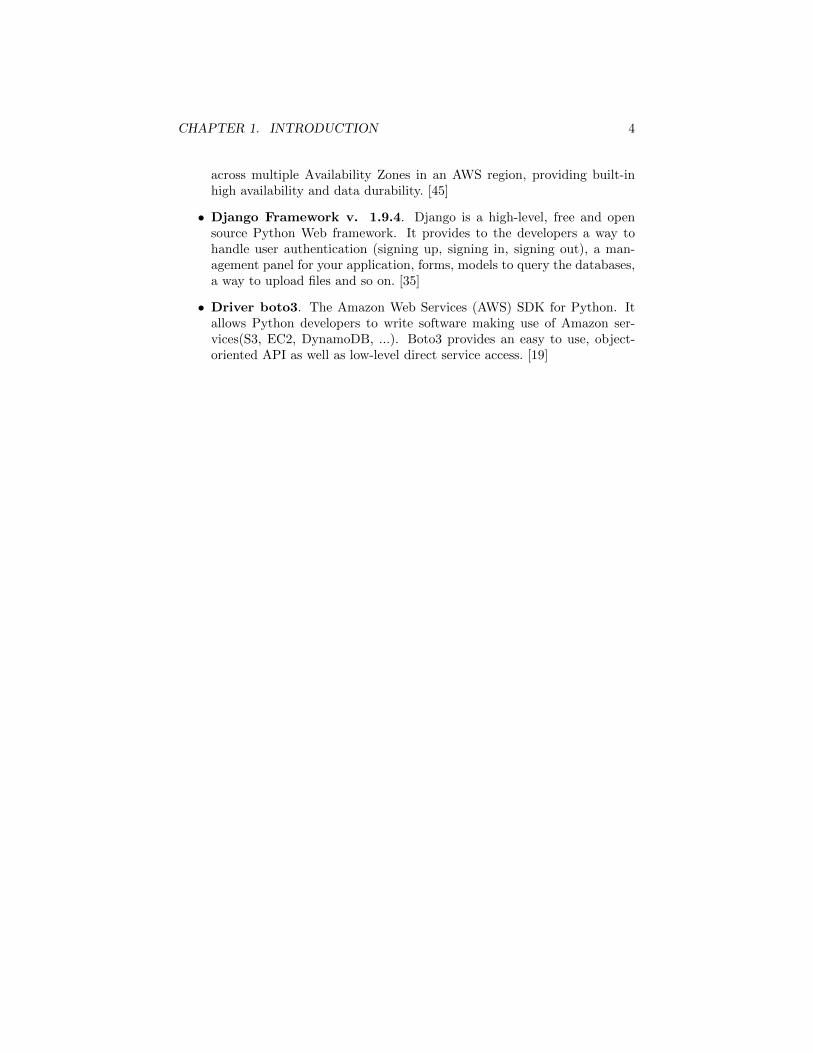
across multiple Availability Zones in an AWS region, providing built-inhigh availability and data durability. [45]
• Django Framework v. 1.9.4. Django is a high-level, free and opensource Python Web framework. It provides to the developers a way tohandle user authentication (signing up, signing in, signing out), a man-agement panel for your application, forms, models to query the databases,a way to upload files and so on. [35]
• Driver boto3. The Amazon Web Services (AWS) SDK for Python. Itallows Python developers to write software making use of Amazon ser-vices(S3, EC2, DynamoDB, ...). Boto3 provides an easy to use, object-oriented API as well as low-level direct service access. [19]

Chapter 2
Background and LiteratureReview
This chapter provides a brief introduction to the Relational Database Man-agement Systems (RDBMSs) with their properties and an overview of NoSQLdatabases presenting some data models and their features. It worths to say thattraditional RDBMS does not have anything wrong, just they were not built todeal with a really huge amount of data and the entrance in the market of NoSQLdatabases with their roughly cheap hardware needs, has designed the necessityof some SQL databases to be converted to NoSQL ones. [12] However, the realgoal of NoSQL is not to reject SQL but instead to be used as alternative datamodel in situation where relational databases do not work well enough.
2.1 Related Work
In [10] A. Diomin and K. Grigorchuk show some useful key criteria to take intoaccount when the choice of a DB is required.Scalability has to be guaranteed since when your application’s traffic rises,rapid scalability upon requests is strictly required to fill up the lack of your DB’scapacity. In the same line, when the system is idle, it has to be able to reducethe used resources. NoSQL DBs provides horizontal scalability by splitting thesystem into smaller components hosted on several physical machines that canbe added on the fly and performs the same operation in a parallel manner.Performance is important to persistently provide low latency regardless datasize or task. ”In general, the read and write latency of NoSQL databases is verylow because data is shared across all nodes in a cluster while the application’sworking set is in memory.” [10]High Availability is necessary because large amount of money could be lostfrom a business at any time the application is down. It is strongly required thepossibility to provide disaster recovery, to perform online upgrades, backups oreasily remove a node for maintenance without affecting the availability of the
5

CHAPTER 2. BACKGROUND AND LITERATURE REVIEW 6
cluster.Ease of deployment since SQL databases own a rigid schema, if the appli-cation change, most probably the DB’s schema will have to change too whileNoSQL DBs are know to be schemaless so this constraint should not be an issueanymore. [44]
In early times there has been many papers studying relationships betweenNoSQL and relational databases providing overviews and showing their charac-teristics, benchmarks and performance. [8, 59]
From [11] NoSQL seems to have a kind of structure that allow to store andprocess large amounts of data of (almost)any type providing high availabilityand being way faster than RDBMS.
Besides all the advantages like speed, better performance and high scala-bility NoSQL may bring into the market, Leavitt in [49] shows that they stillpresent some drawbacks when compared with relational databases. He espe-cially observed that even though they are fast in performing simple operations,they becomes tedious when operations get more complex.
Nowadays, security has becoming more and more an undertaken featurebeing on of the most considerable concern for IT Enterprise Infrastructures.Unfortunately, the weakness of security in NoSQL is mainly due to the fact thattheir designer focuses on other purposes than security and Authentication/En-cryption where implemented are almost absent. [15]
The research made by Indrawan-Santiago in [47] had the intention to gathertogether some basic comparisons that could be made among NoSQL DBs andagainst relational databases. The research that eventually shown the comple-mentarity between NoSQL and RDBMS included transaction and data model,indexing, sharding, support for ad-hoc-queries and license type.
In [27] a comparison between relational and NoSQL databases had beendescribed, precisely by using Oracle and MongoDB. From the study came upthat the query time calculated performing an insert operation was a factor higherin Oracle than in MongoDB while performing delete and updates took severalfactors more than MongoDB.
2.2 Overview of RDBMS
A database can be considered as an organized collection of data [26], a hugelibrary where every shelve is represented by a table containing records, splitby attributes (columns). The system which is in charge to manage all theinteraction with the database is called Database Management System(DBMS)and it is represented by an organized set of facilities to controls the organizations,accesses, retrieval of data and to maintain one or more storages. [26] DBMSs canbe classified based on their criteria in Data Model, User Numbers and DatabaseDistribution.
• Data Model comprehends several types:
– Relational Model(RDBMS): nowadays the most widely used data

CHAPTER 2. BACKGROUND AND LITERATURE REVIEW 7
model. It uses structures consistent with the first-order predicatelogic based on the relational model proposed by E. F. Codd in 1970[28] and the one it has been used in this work. [4]
– Hierarchical Model: data is organized in a rooted-tree-like struc-ture (no cycles) and stored as records linked together by links. Therelationships between a parent and a child must be one-to-many orone-to-one and the database schema is represented as a collectionof tree-structure diagrams where every diagram has one single in-stance of a database tree rooted at a dummy node. This model’sstructure was the base of one of the firsts database models used andimplemented in IBM’s Information Management System(IMS). [3]
– Network Model: it can be seen as a generalization of the hierarchi-cal model where each data object can have multiple parents and eachparent object can have multiple children forming a lattice-type struc-ture in contrast to the tree-like structure of the hierarchical model.It is useful to represents real-world data relationship more naturallyand under less constrained environment. [24]
– Object-Relational Model(OODBMS): it has been introduced inrecent years and it is one of the newer and more powerful models ofall the aboves. Information are represented by objects and it addsobject-oriented concepts to facilitate data modeling and its relation-ships. [2]
• User Numbers: it can be distinguished in DBMS which supports oneuser at a time(single-user), or in a DBMS, which supports multiple usersconcurrently(multiuser). [63]
• Database Distribution: it in turn is divided in four main distributions:
– Centralized systems: the database and DBMS are both placed inthe same site used from other systems too.
– Distributed database system: the database and DBMS are placedin different locations each one connected to each by a computer net-work.
– Homogeneous distributed database systems: make use of thesame DBMS from multiple locations.
– Heterogeneous distributed database systems: it makes avail-able additional common software in order to support data exchangeamong locations that make use of different DBMS software.
Further and in-depth description of these models is beyond the scope of thepresent work. However, the next section will show a bit more in details theRelational Model that is on protagonist of this research.

CHAPTER 2. BACKGROUND AND LITERATURE REVIEW 8
Figure 2.1: Example of a relational model
2.2.1 The Relational model
Over the years the relational database management systems (RDBMS) havebeen the leading technology in the IT world. The relational model is funda-mentally based on two mathematical components: first-order predicate logic [4]and the theory of relations. This approach of using the relational systems in allscenarios came under scrutiny with the introduction of the web. The relationaldata model works well with the traditional applications where the data is notmassive and distributed. Despite being on top for several years the capabilityof the RDBMS for processing and handling large amount of data remains inquestion.
The relational model, as discussed in [28] was developed to assign some is-sues like removing data consistency, hiding from the users the organization ofthe data in a machine and to protect users’ activities (and applications’ pro-grams) from growing data types and internal data changes. The data structurein a relational model is made by several components identified as relation, en-tity, domain, attribute(column), tuple, and attribute’s value. As in fig. 2.1 arelation(table) is represented by the Cartesian product of a set of records(rowsor tuples) identified by a name and is then intended to represent data throughtables composed by rows and columns. A schema is a description of the data interms of data model.
Basically, a database is represented by a collection of one or more relations,where each one is based on a relation schema and a relation instance. Therelation schema is used to specify relations’ name, attributes’ names Ai andattributes’ domains(types) Di while the relation instance is a finite set of tuples.[4]
In a relation schema denoted by R(A1:D1, A2:D2, . . . , An:Dn), R stands forthe relation name while A1, A2, . . . , An represents a list of attributes and eachDi indicates the domain of the related attribute(column).
Eventually, a Relational Database is a collection of relations with dis-tinct relation names and Relational Database Schema is the collection ofrelations’ schemas in the database and Integrity Constraints.
In an abstract level, tables represent entities like the ones in fig. 2.2 thatare user and food while user favorites represents the relation between these twoentities. The relational style is very useful to design a database schema mappingreal world objects as database tables and relations among them expressed by

CHAPTER 2. BACKGROUND AND LITERATURE REVIEW 9
Figure 2.2: Example of a database schema
primary and foreign key to link tables together. [4]
2.2.1.1 Integrity Constraints: the concepts of Primary key and For-eign key
A primary key is represented by a single column or a combination of columns(inthis case is called composite key) and it identifies uniquely a tuple in a relation.In a composite key, every column taking part to the key, should be a foreignkey, but not necessarily [31]. If more attributes could identify the tuples, suchattributes are called candidate keys.
A foreign key is again a column or a set of columns in one relation that makea reference to the primary key in another table. As example, in fig. 2.2 the tablevg user favorites maintains two foreign keys that are food id and user id.
Every table must satisfy several constraints in order to be a valid relation.The following main classes of integrity constraints are described in [26,31]:
• Entity Integrity Constraint: every primary key has to be unique andnot to contain NULL values since they are used to identify every tuple ina relation.
• Referential Integrity Constraint states that if a relation has a foreignkey, this one must refer to an existing tuple. It is intended for maintain-ing consistency between tuples of two tables. Records from a table, forinstance, cannot be deleted/changed if matching records exist in anothertable.
• Domain Constraint designates and important condition to be satisfied,”every attribute value inserted in a specific column must be in line withthe domain specified for such column”.
Other types of constraint are extensively explained in [26] section 5.3.∗.
2.2.1.2 The concept of Normalization
One of the main goals of relational database design is to normalize a rela-tion schema together with a set of data dependencies into an suitable normal

CHAPTER 2. BACKGROUND AND LITERATURE REVIEW 10
form [31] to eliminate issues related to inconsistency and redundancy improvingdata integrity. E. F. Codd introduced the term normalization and what is wellknown as First Normal Form(1NF) that consist of eliminating repeating databy creating a new table for each group of related data identified by a primarykey. [28] Later on he also defined the Second Normal Form(2NF) and ThirdNormal Form(3NF) [29] that are presented as the following:
• 2NF: if the table has some values which are the same for multiple recordsthen move them into a new table and link the two tables through a foreignkey.
• 3NF: keep in the table only fields that depend on the primary key, atmaximum put non depending fields into another table.
A few years later together E. F. Codd and Raymond F. Boyce introduced a formthat looks like slightly strong than 3NF called Boyce-Codd Normal Form .[30] This form ensures that no redundancy can be detected using functionaldependency [34] and every candidate keys do not have any partial dependencyon other attributes.
All these normal forms are someway related: every relation in BCNF is alsoin 3NF which in turn is in 2NF and every relation in 2NF is in 1NF.
2.2.2 The ACID properties
A transaction is a very small unit and it may contain many other low-level tasks.RDBMSs ensure four properties under the name of ACID properties in orderto guarantee completeness, data integrity and to get transaction reliability inconcurrent accesses and system failures. ACID stands for [4, 26]:
? Atomicity: based on ”all or nothing” statement. Every transaction mustbe considered as an atomic unit meaning that either all or none operationsare accomplished.
? Consistency: every completed transaction brings the database from aconsistent state to another so any values’ changes in an instance are con-sistent with other values’ changes in the same instance.
? Isolation: every transaction is isolated, so in case of concurrent transac-tions, the system is able to prevent conflicts and it will eventually end inthe same state as if the transactions would have been performed serially.
? Durability: every changes applied to the database once a transactionhas been committed, it will persist in the database in any case of powerfailures, errors and crashes.
RDBMs achieve atomicity and durability by a log file that keeps track ofany updates performed by any transaction so that if a error/failure occurs thedatabase rolls back the transaction itself unbinding the update. Using a log filegives the advantage that nothing in memory has to be maintained and in case of

CHAPTER 2. BACKGROUND AND LITERATURE REVIEW 11
failure the rollback can be performed when the system restarts. If a transactionsucceeds but the crash comes up right before the data was saved to the diskthen all the updates can be started over through the log file.
Isolation is usually obtained through ”locking”. Locks can be shared by anynumber of transactions that only want to read the data but not to update it(orvice versa). If a transaction is read-locked then no write-locks can be performedon the same transaction. If the transaction is write-locked no other write/readlocks can do anything until the lock has been released.
2.2.3 SQL Language
SQL, also known under the name of Structured Query Language, is a compre-hensive query language based on Codd’s concepts built from a simplified versionof DSL/Alpha that was previously developed by IBM [25].
It represents a combination of Data Definition Language(DDL, usedto define schemas), View Definition Language(VDL, used to specify userviews and their mappings to the conceptual schema) and Data ManipulationLanguage(DML,used to define set of operations to manipulate data) and itmainly allows to perform query language to define both conceptual and externalschema, user and application views as results of predefined queries. [34]
Relational DBMSs make totally use of it to query data in databases’ rela-tions. The following example, based on the relations in fig.2.2, shows how simpleis to query a table with SQL:
1 SELECT ∗2 FROM vg use r U3 WHERE U. surname = ”Ross i ”
This example allows to retrieve all the users with surname equal to ”Rossi” fromthe relation vg user.
2.2.4 Amazon RDS for MariaDB
Amazon RDS(Relational Database Service) is a solution that requires no dealingwith administration and maintenance since RDS is born to be a fully functionalalternative to common hardware databases. It is fast, scalable and can be repli-cated among Availability Zones(AZs) in order to get a better level of accessibilitybecause low-latency network connectivity is provided towards the other Avail-ability Zones in the same region. As well, your applications can be protectedfrom failure in a single location if just they are launched from separated Avail-ability Zones. RDS supports the management of several well know databaseengines like MySQL, PostgreSQL, Amazon Aurora, MariaDB, Microsoft SQLServer and Oracle. [46]
The basic ”building block” of Amazon RDS is the DB instance which rep-resent an isolated database environment in Amazon cloud. Each DB instance

CHAPTER 2. BACKGROUND AND LITERATURE REVIEW 12
can own from 5GB to 6TB of associated storage capacity. Storage capacitycomes int three different ways that also have distinct performances and costs:Magnetic, General Purpose (SSD), and Provisioned IOPS (SSD). [46]
Moreover, each DB instance can be launched in various Availability Zonesand Amazon accordingly provisions a ”synchronous standby replica of your DBinstance in a different Availability Zone” to minimize latency in case of systembackups, to supply data redundancy, fail-over support and so on. [46]
More detailed and fully documented information about Amazon RDS canbe found in [46].
2.3 Sharding
Every application’s developer or DB’s administrator is aware that if the loadof transactions and DB’s size increase linearly, the response times rise logarith-mically. Performance and scalability mainly depends on how database manage-ment systems are built and in turn they rely on Memory, CPUs and Disks.
Figure 2.3: Example of Sharding
Of course, it is not enough in-crease only one of these componentsto reach performance improvementsor scalability but if more processingcores are provided also memory andhard drive capacity need to be in-creased.
Due to the way they are struc-tured, relational databases usuallyscale vertically, a single server hoststhe entire DB ensuring acceptableperformance for cross-table joins andtransactions. This places limits onscalability, gets expensive and adds a
few failure points for DB infrastructure.The term Sharding(or partitioning) represents the approach under which
data can be stored over many thousands of computers to improve the throughputand the overall performance especially if related to high-transactions.
Instead of storing data in a DB on one single machine, it is partitioned insmaller DBs called Shards across a cluster of nodes allowing to structure theDB with smaller index size, smaller working set and improving the handle ofwriting operations. Nodes can be added to the cluster to increase both capacityand write/read operation performance, contrary, if the demands decrease thesize of a sharded DB cluster can be reduced. This ability goes under the nameof Horizontal scalability.
Relational DBs do not provide the ability to scale horizontally but Shardingcould be achieved through Storage Area Networks(SANs) and other complexarrangements for making hardware act as a single server.
The concept of Database Sharding has been gaining popularity over the past

CHAPTER 2. BACKGROUND AND LITERATURE REVIEW 13
several years, due to the high increase in transaction volume and size of businessapplication DBs.
However, a couple of drawbacks can be found in relational database withthe use of operations like Joins, used to combine associated tuples from tworelations into single ones [34]. It is not difficult to realize that, as joins workwith two relations, performing such operation in a sharded DB would requiremany search requests to all the nodes containing items from one of the tworelations causing high network traffic. Moreover, making use of sharded DB,the probability of node (or connection) failures increases hand in hand with theincrease of the number of used nodes. Relational databases are not well suitedto scale in this fashion, they look more appropriate towards vertical scaling (e.g.adding more memory, storage, ...) but of course it rises the limit of the numberof resources that eventually can fit inside a machine. There could come a pointwhere horizontal scaling becomes the only option.
2.4 Replication
Figure 2.4: Example of Replication
Regardless the evident advantage ofadded performance DB, replication isrecommended over sharding as it pro-vides redundancy and increases dataavailability. Having multiple copies ofdata in different DB servers allows notonly to protect the DB from loss on asingle servers but also to recover fromhardware failures or service interrup-tions and to increase the locality andavailability of data in distributed ap-plications. With additional replicasof the data, each one can be dedi-cated to different tasks like disasterrecovery, reporting, or backup. e.gwith more and more page requests,more and more reads are forwardedand replication may be used to in-crease read capacity, replicate the DB to read servers in such a way that theload balancer can forward writes operations to master and reads to the readserver.
Is common use to replicate database to different locations(or regions) inorder to decrease latency in requests since data will be closer to the user. Inany case, write operations are the drawback in replicated database environmentsbecause every write has to be forwarded to each node supposed to store suchdata item. [1] Depending on the desired level of availability and consistency aDB requires, there are two recommended ways to perform such operation:
• Commit the write towards all the nodes.

CHAPTER 2. BACKGROUND AND LITERATURE REVIEW 14
• Commit it towards one or a limited number of nodes then send it asyn-chronously to all the others.
2.5 Eventual & Strong consistency
In talking about consistency the scenario where every entity owns a copy of thedata object is take into consideration. Conflicts can arise because each node canperform updates on its own copy and users connected to different nodes maysee different values.
• Eventual Consistency: (also called weak consistency) each node com-municates to each other its own changes and eventually after a fixed periodof time without any other value’s modification they agree on a definitivevalue. The update operation here ends as soon as the local copy of theitem is updated then it is ”broadcasted” to all the other nodes. Thesystem does not guarantee that at every access the most updated valuewill be picked up during such period of time called inconsistency window.Moreover, in case of data replication, during the inconsistency window theprocess that writes the values could also get a non updated version of thedata. [62]
• Strong Consistency: when a user makes an update to the data thesystem does not return anything instantaneously indeed it locks all theaccesses to any copy of the data until all nodes have agreed on such up-dated value. Doing so every user will always read the same version of thedata at the same time. [41]
2.6 NoSQL Databases
There are a lot of NoSQL database solution to take into account and it is hardto keep track about where they shine, where they fail or even where they aredifferent, as implementation details change quickly and feature sets evolve overtime. [10] A common feature is their capability to store big data and work withCloud computing systems. Many of them are able to offer horizontal scalabilityand provide higher availability than relational databases by sacrificing queryingcapabilities and consistency guarantees. Every outstanding database has beendesigned for a specific class of application or in order to achieve a precise solutionbased on clear-cut system properties’ requirements. The reason behind thepresence of such large number in different database systems would be prettyclear thinking that any system would struggle to achieve all desirable propertiesat once.
2.6.1 NoSQL data models
The most common way to make a distinction among NoSQL databases is basedon how they store and allow access to data. In the following subsections five dif-

CHAPTER 2. BACKGROUND AND LITERATURE REVIEW 15
ferent data-models’ categorizations of NoSQL DBs will be presented and brieflydescribed [47].
2.6.1.1 Key-value store
Key-value stores are the simplest among the NoSQL category and consist of aset of key-value pairs with unique keys. They work similarly to a traditionaldictionary or hash table(where values are retrieved by using the key) but dis-tributing keys and values among a set of physical nodes.
Figure 2.5: Example of key-value store
The data is stored in two parts,the real data that represents the valuestored(string, integer, list, dictionaryand so on) and a string represent-ing the key to reference that value.Their very simple abstraction makesthe database easy for partitioning andquerying the data reaching in generallow latency and high throughput.
However, due to their simplicity,Key-value stores just support basicCRUD (Create, Read, Update andDelete) and conditional operations.They are not suitable for applicationswith complex query operations likejoin or range queries. Due to thisdrawback, often data has to be ana-
lyzed in the application code to extract information, where queries more complexthan simple lookups are required.
Key-value stores turns out to be in general good solutions if the applica-tion presents only one kind of object and the main operations are look ups ofobjects based on one attribute. Examples of widely used Key-value stores areDynamoDB [45], Project Voldemort [51] and Redis [60].
2.6.1.2 Document store
Figure 2.6: Example of a document
A Document-oriented DBs use a doc-ument oriented model extending thebasic key-value store concept andstoring data in the fashion of semi-structured formats such as JSON,XML or PDF [9]. Documents are ad-dressed by using a key(simple stringor a string that refers to a pathor URI) that represent a sort ofID and uniquely identifies a docu-ment. To some extent every docu-

CHAPTER 2. BACKGROUND AND LITERATURE REVIEW 16
ment looks similar to a record in re-lational databases but way more flex-ible because they are schema less. While every record in a relational databasemay contain data in each field or it may leave unused field empty but still there,a document store is schema less and so every document may contain differentdata as different sized fields, they may be similar to each other document butdo not have to be the same. They also allow to wrap key-value pairs in a doc-ument and due to this their complexity becomes slightly higher than key-valuestores. [9] It is not advised to make use of a document-store if the data own a lotof normalization and relations [9], but, if the data does not need to be stored inuniform size or the domain model can be partitioned in some parts then a doc-ument store looks the right choice. MongoDB [54] and Apache CouchDB [40]are two of the most known and used document-stores nowadays.
2.6.1.3 Graphs database
Figure 2.7: Example of Graph data struc-ture1
Graph databases use the graph the-ory approach to store entities and re-lationship among these entities. Thegraph is made by two components,nodes, representing the objects and,edges, representing the relationshipsbetween those objects(interlinked el-ements). Nodes also have propertiesand are organized by relationships al-lowing to find interesting patterns be-tween the nodes. To optimize thelookups Graph DBs use a so calledindex free adjacency technique where every node has a direct pointer to the ad-jacent node. With this technique millions of records can be traversed. However,it is very difficult to achieve sharding because it is very hard to cluster them.Graph databases are widely used in applications like social networks, bioinfor-matics, security and access control, content management etc. Neo4j [55] andTitan DB [43] are some of the notable Database-as-a-Service(DBaaS) providerusing graph data stores.
2.6.1.4 Wide-column store
The main feature of Wide-column stores is that instead of storing data byrows(as it happens with relational databases), they store data in column fami-lies that are nothing more than groups of related data often accessed together,in this manner, data can be aggregated rapidly with less I/O activity.
This kind of databases look like a distributed multidimensional sorted mapwhere columns are defined for every row (key-value pairs) in such a way that
1Thanks to https://s3.amazonaws.com/dev.assets.neo4j.com/wp-content/uploads/
data-modeling-5.png

CHAPTER 2. BACKGROUND AND LITERATURE REVIEW 17
any row can have different columns and any number column can be added toany row. [9]
To make things more clear, as shown in fig.2.8, a column family could be seenas a container of rows(in RDBMS) everyone consisting of multiple columns andeveryone identified by a key. This structure offers flexibility in data definitionand allows to apply data compression algorithms per column.
Figure 2.8: Simple example of Column-store
The storage scheme is identifiedby both row keys to identify rows andcolumn keys which in turn identifiescolumns [14]. On disk data valuesare stored from the same column fam-ily and from the same row in lexi-cographic order of their keys in sucha way that they result physically co-located. However, to retrieve a row,a single lookup is not enough instead,
a join from the columns of all the column families is required.Examples of well known Wide-column store are Google Big Table [5] and
Cassandra [39].
2.6.2 The CAP Theorem
In contrast to the ACID transaction properties respected by relational databases,NoSQL databases trusts on the CAP theorem exposed in 2000 during a Sym-posium on Principles of Distributed Computing. The theorem presented by EricBrewer and later confirmed by Gilbert and Lynch in [42] brought to the lightan upper bound based on a trade-off between:
• Availability(A): data must always be available,
• Consistency(C): data is always the same no matter which replication orserver,
• Partition Tolerance(P): database is able to work even in presence ofmachine/network failures.
According to this theorem, in distributed systems, only two of the three prop-erties could really be guaranteed at a specific moment in time [16]. Brewerstated that in partitioned system having both consistency and availability wasnot fully possible because in case of a host’s failure that will lose the connectionwith the other nodes, for instance, it will have to choose if to preserve avail-ability(AP) keep processing requests form clients and so violating consistencyor to guarantee consistency rejecting clients’ requests and sacrificing system’savailability(CP). Another scenario is the one with a single-node system whereavailability and consistency can be preserved at the price of lacking completelyin partition tolerance(CA) [16]. Depending on the use cases, the most important
CHAPTER 2. BACKGROUND AND LITERATURE REVIEW 18
combination needs to be chosen. When the consistency of data is crucial, rela-tional DBs should be used but when data is distributed across multiple servers,such consistency becomes hard to achieve.
Cap theorem has then evolved into what is now known as BASE principlewhich means Basically Available, Soft State and Eventual Consistency and thatis characterized by high availability of data, while sacrificing its consistency[56,57].
2.6.3 Query language
Despite relational DBs that use the SQL language to make queries, NoSQL DBsdo not have any real standard query language. Most of the NoSQL DBs havecreated their own query language, some examples are MongoDB which usesmongo query language , Cassandra that make use of CQL(Cassandra QueryLanguage) or boto3 used by DynamoDB and S3.
2.6.4 Overview of Amazon DynamoDB
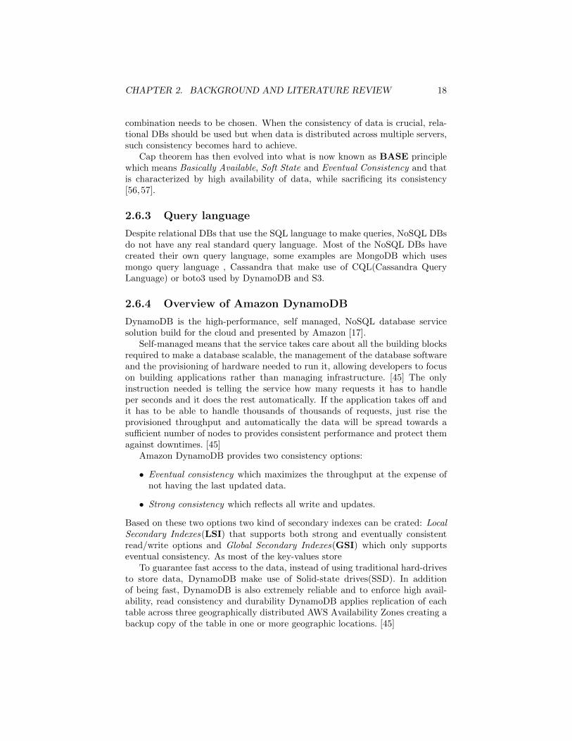
DynamoDB is the high-performance, self managed, NoSQL database servicesolution build for the cloud and presented by Amazon [17].
Self-managed means that the service takes care about all the building blocksrequired to make a database scalable, the management of the database softwareand the provisioning of hardware needed to run it, allowing developers to focuson building applications rather than managing infrastructure. [45] The onlyinstruction needed is telling the service how many requests it has to handleper seconds and it does the rest automatically. If the application takes off andit has to be able to handle thousands of thousands of requests, just rise theprovisioned throughput and automatically the data will be spread towards asufficient number of nodes to provides consistent performance and protect themagainst downtimes. [45]
Amazon DynamoDB provides two consistency options:
• Eventual consistency which maximizes the throughput at the expense ofnot having the last updated data.
• Strong consistency which reflects all write and updates.
Based on these two options two kind of secondary indexes can be crated: LocalSecondary Indexes(LSI) that supports both strong and eventually consistentread/write options and Global Secondary Indexes(GSI) which only supportseventual consistency. As most of the key-values store
To guarantee fast access to the data, instead of using traditional hard-drivesto store data, DynamoDB make use of Solid-state drives(SSD). In additionof being fast, DynamoDB is also extremely reliable and to enforce high avail-ability, read consistency and durability DynamoDB applies replication of eachtable across three geographically distributed AWS Availability Zones creating abackup copy of the table in one or more geographic locations. [45]

CHAPTER 2. BACKGROUND AND LITERATURE REVIEW 19
DynamoDB does not have any limits on data storage per user, nor anymaximum throughput per table.

Chapter 3
Framework design and DBengines
Application developers surely have plenty of experience in the use of relationaldatabases and SQL. Besides underling all the differences, working with NoSQLdatabases brings to discover that eventually they have even more similaritiesthan it is thought.
The design and architecture of data models are key factors in the flexibility ofany database considering that they determine how data is stored, organized andcan be manipulated. Understanding differences and similarities between NoSQLand RDMS database engines, their data models and how they work might helpto better interpret the results obtained from our benchmarking analysis. Forinstance, it could be interesting to find out that the way a DB stores its datacould impact the query time needed to retrieve such data in respect to the otherdatabase. For this purpose, this chapter aims to describe the data models usedby Amazon RDS for MariaDB and Amazon DynamoDB comparing SQL basicstatements with their equivalent NoSQL operations.
3.1 How do DBs store data?
In relational databases every information is supplied through models explainedin section ( 2.1). By using an user-oriented approach, SQL queries work outpretty well assuming that data would be aggregated in one place to give allthe needed information at once. However, creating the DB schema providingtransactional guarantees and maintaining this kind of pattern requires a lot oftime and effort.
3.1.1 Amazon RDS for MariaDB
The basic building blocks for Amazon RDS are represented from the so calledDB instances. Each instance is an isolated database environments in the cloud,
20

CHAPTER 3. FRAMEWORK DESIGN AND DB ENGINES 21
running its own DB engine with its features and supporting from 5GB up to6TB of associated storage capacity [46]. Amazon RDS supports various DBengines like MySQL, MariaDB, PostgreSQL, Oracle, and Microsoft SQL Server.However, this work has been focused only on MariaDB to represent the relationaldatabase category.
The data-structure in DBMS varies considerably, from fixed/variable lengthrecords of structured data to variable length records of opaque data, hash tableentries and nodes of tree indexes(e.g. B-Tree, R-Tree, ...). Most commonlyRDBMSs use variations of B-Tree as organizational structure for informationstorage to separate user applications from the physical database. Some examplescould be found with MySQL which uses B+ tree to store data indexes, InnoDBstores both data and index file into the memory while MyISAM maintains onlythe index file, MariaDB instead uses a fork of InnoDB called Percona XtraDBwhich incorporates InnoDB’s ACID-compliant design and MVCC architecturebuilding greater scalability and providing a good tuning degree. [52]
Figure 3.1: Example of B-tree structure
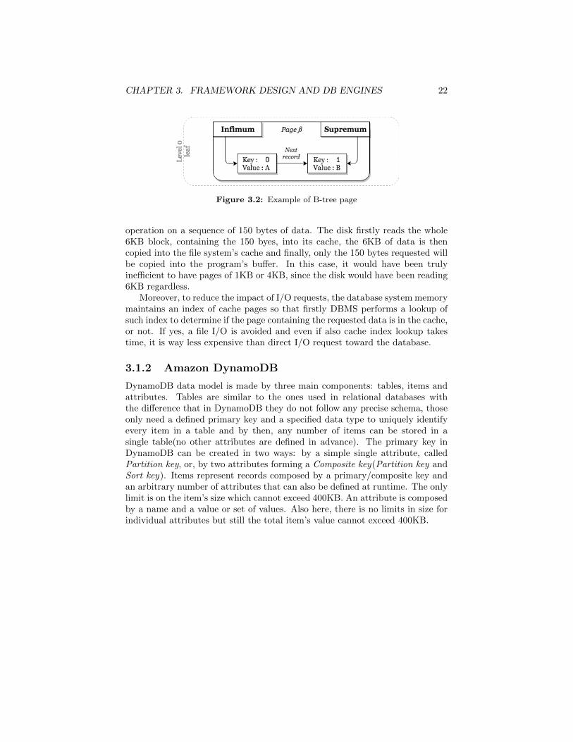
B-Trees [7] owns a particular structure well suited to store large sorted dic-tionaries on a fixed size blocks called pages(fig. 3.2). In each page, Infimumand Supremum point respectively to the lowest key value and the highest keyvalue inside the page itself. Every page is linked with the previous and the nextpointers in ascending order by key while each record is only linked to the nextone again in ascending order by key. Beside the Leaf Level 0, fig. 3.1 shows thatthere are other two levels, respectively Internal Level 1 and Root Level 2. Bothinternal and root level point to the lower key of the child and maintain the nodepointer which is represented by the child page number.
Pages are in general maintained in a storage device such as HDD or SSD.In order not to lose any required data, it is advised to adjust each page sizeaccording to the device blocking factor, since that, when a request is made, thedisk always read/write an entire block at a time even if the data requested isnot large.
Supposing to have a disk block size of 6KB and we want to forward a read
CHAPTER 3. FRAMEWORK DESIGN AND DB ENGINES 22
Figure 3.2: Example of B-tree page
operation on a sequence of 150 bytes of data. The disk firstly reads the whole6KB block, containing the 150 byes, into its cache, the 6KB of data is thencopied into the file system’s cache and finally, only the 150 bytes requested willbe copied into the program’s buffer. In this case, it would have been trulyinefficient to have pages of 1KB or 4KB, since the disk would have been reading6KB regardless.
Moreover, to reduce the impact of I/O requests, the database system memorymaintains an index of cache pages so that firstly DBMS performs a lookup ofsuch index to determine if the page containing the requested data is in the cache,or not. If yes, a file I/O is avoided and even if also cache index lookup takestime, it is way less expensive than direct I/O request toward the database.
3.1.2 Amazon DynamoDB
DynamoDB data model is made by three main components: tables, items andattributes. Tables are similar to the ones used in relational databases withthe difference that in DynamoDB they do not follow any precise schema, thoseonly need a defined primary key and a specified data type to uniquely identifyevery item in a table and by then, any number of items can be stored in asingle table(no other attributes are defined in advance). The primary key inDynamoDB can be created in two ways: by a simple single attribute, calledPartition key, or, by two attributes forming a Composite key(Partition key andSort key). Items represent records composed by a primary/composite key andan arbitrary number of attributes that can also be defined at runtime. The onlylimit is on the item’s size which cannot exceed 400KB. An attribute is composedby a name and a value or set of values. Also here, there is no limits in size forindividual attributes but still the total item’s value cannot exceed 400KB.

CHAPTER 3. FRAMEWORK DESIGN AND DB ENGINES 23
Figure 3.3: DynamoDB data model
Although relational databases support many data types, DynamoDB at-tributes support just a few: scalar data types (String, Binary, Number, Boolean,and Null), multivalued data types (string set, binary set and number set) anddocument (List and Map). A simple data model with some of the describedcomponents is shown in fig. 3.3.
Every table’s data is stored in Partitions that are nothing more than allo-cation of storage in a SSD.
Figure 3.4: Example of table’s partitions
The distribution among the partitions is based on the partition key value andthe partitioning logic depends upon two things: table size and throughput. Toreach the full amount of the specified provisioned throughput, since DynamoDBis ”optimized for uniform distribution of items across a table’s partitions, nomatter how many partitions there may be” [23], it is strongly recommended tocreate tables where partition keys have very distinct values in such a way tomaintain the workload smoothly spread across those partition key values anddistribute the requests across partitions.
Amazon documentation explains that ”if a table has a very small numberof heavily accessed partition key values then request traffic is concentrated on asmall number of partitions. If the workload is heavily unbalanced, it means thatit is disproportionately focused on one or a few partitions and so the requestswill not achieve the overall provisioned throughput level” [23]. Generally, thethroughput is more efficiently utilized when the access ratio of partition key

CHAPTER 3. FRAMEWORK DESIGN AND DB ENGINES 24
values to the total number of partition key values, in the table, increases.During the creation of a new table the user is required to specify the provi-
sioned throughput capacity that such table needs to be reserved for reads(readcapacity units) and writes(write capacity units) [45]:
• One Read Capacity Unit allows to have one strongly consistent(or twoeventually consistent) read/s per second towards items of size up to 4KB.Read capacity unit depends either on item size and whether the user needsstrongly or eventually consistency. In case it is required to read largeritems, read capacity units will need to be increased(at some price).
• One Write Capacity Unit depends on the item size since it allows towrite items up to 1KB per second. If the item that needs to be written islarger than 1KB than write capacity units need to be increased.
Exception is done for table with Global Secondary Indexes(GSI) that will con-sume double capacity units, one to write in the table and one to write in theindex. It is worth to specify that DynamoDB estimates the number of consumedwrite/read capacity units based on item size and not on the amount of data thathas to be stored or returned to an application. ”The number of capacity unitsconsumed will be the same whether you request all of the attributes (the defaultbehavior) or just some of them using a projection expression” [20].
Once the table is created DynamoDB automatically allocates a sufficientnumber of partitions to it in order to be able to handle the specified provi-sioned throughput(every single partition supports at maximum 3000 read ca-pacity units, 1000 write capacity units and approximately 10GB of data) andfrom that moment on all the concerns about partition is fully managed by Dy-namoDB [23]. After the creation, data is also automatically replicated acrossmultiple Availability Zones within an AWS region. In the case that more stor-age is needed because provisioned throughput exceeds the limit a partition cansupport or the partition’s capacity is fully used, then DynamoDB will allocateadditional partitions.
To see how many partitions a new table would require in order to accommo-date the provisioned throughput the following equation can be used:
#ThroughputPartitions =readCapacityUnits
3000+writeCapacityUnits
1000(3.1)
To calculate the number of partitions to accommodate the table size indeed:
#PartForTableSize =TableSize(GB)
10(GB)(3.2)
Eventually the total number of partition to be created is given by the equation:
#Partitions = MAX(#ThroughputPartitions|#PartForTableSize) (3.3)

CHAPTER 3. FRAMEWORK DESIGN AND DB ENGINES 25
Example 1:Supposing we are required to create a new table of about 20GBin size with 600 read capacity units(rcu) and 600 write capacityunits(wcu), the initial number of partitions required would be as follow:
#ThroughputPartitions =600
3000+
600
1000= 0.8→ 1
#PartForTableSize =20
10= 2
#Partitions = MAX(1|2) = 2
Since it has been created DynamoDB adopts a combination of several wellknown approaches to obtain such a performing system. It reaches uniform datapartitioning through a consistent hashing algorithm and ensures consistency bymaking use of object versioning and quorum techniques to preserve consistencyamong the replicas [33]. The DynamoDB system is also properly balancedthanks to its symmetric structure made by a ring of nodes where none of themis master and none of them has extra responsibilities or performs extra work.
3.2 Database manipulation
Once the database and tables are created and populated with the data, everyuser must be able to manipulate such data and tables as desired. Typicalmanipulations operations involve Update(Insertion, Deletion, Modification) andRetrieval operations and relational databases as NoSQL have different ways toperform them.
3.2.1 Insert operation
The purpose of an insert operation is to add one or more items to an existingtable. An interesting feature is the fact that after an INSERT statement editsare non permanent until a COMMIT statement is issued since SQL databases aretransaction-oriented rather in Amazon DynamoDB, every action is permanentonce it replies with an HTTP 200 status code.
3.2.1.1 MariaDB
Relational databases present a two-dimensional data structure composed of rowsand columns. The relation’s name with a list of attributes values have to beprovided and listed in the same attributes’ order as the one used during theCREATE TABLE command. Only the values of attributes created with theclause NULL or DEFAULT can be omitted. Some RDBMS also support semi-structured data with native JSON or XML data types but it mainly depends
CHAPTER 3. FRAMEWORK DESIGN AND DB ENGINES 26
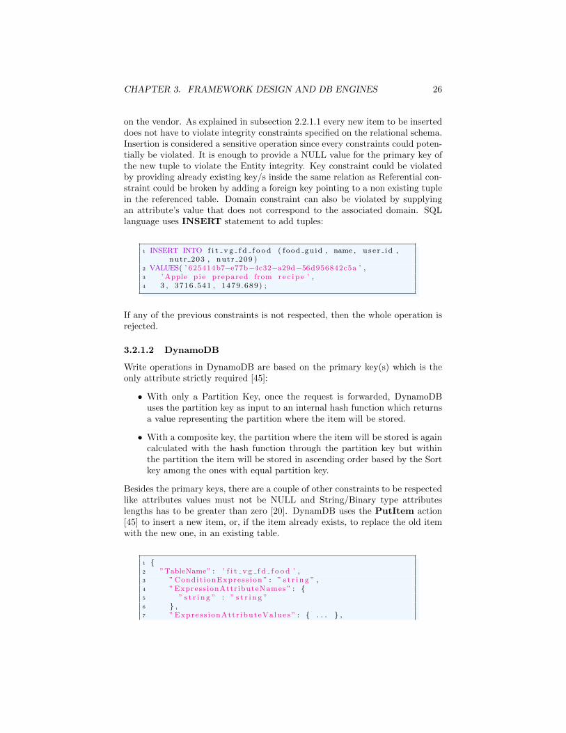
on the vendor. As explained in subsection 2.2.1.1 every new item to be inserteddoes not have to violate integrity constraints specified on the relational schema.Insertion is considered a sensitive operation since every constraints could poten-tially be violated. It is enough to provide a NULL value for the primary key ofthe new tuple to violate the Entity integrity. Key constraint could be violatedby providing already existing key/s inside the same relation as Referential con-straint could be broken by adding a foreign key pointing to a non existing tuplein the referenced table. Domain constraint can also be violated by supplyingan attribute’s value that does not correspond to the associated domain. SQLlanguage uses INSERT statement to add tuples:
1 INSERT INTO f i t v g f d f o o d ( food guid , name , u s e r i d ,nutr 203 , nutr 209 )
2 VALUES( ’ 625414b7−e77b−4c32−a29d−56d956842c5a ’ ,3 ’ Apple p i e prepared from r e c i p e ’ ,4 3 , 3716 .541 , 1479 .689) ;
If any of the previous constraints is not respected, then the whole operation isrejected.
3.2.1.2 DynamoDB
Write operations in DynamoDB are based on the primary key(s) which is theonly attribute strictly required [45]:
• With only a Partition Key, once the request is forwarded, DynamoDBuses the partition key as input to an internal hash function which returnsa value representing the partition where the item will be stored.
• With a composite key, the partition where the item will be stored is againcalculated with the hash function through the partition key but withinthe partition the item will be stored in ascending order based by the Sortkey among the ones with equal partition key.
Besides the primary keys, there are a couple of other constraints to be respectedlike attributes values must not be NULL and String/Binary type attributeslengths has to be greater than zero [20]. DynamDB uses the PutItem action[45] to insert a new item, or, if the item already exists, to replace the old itemwith the new one, in an existing table.
1 {2 ”TableName” : ’ f i t v g f d f o o d ’ ,3 ”Condit ionExpress ion ” : ” s t r i n g ” ,4 ”Express ionAttr ibuteNames ” : {5 ” s t r i n g ” : ” s t r i n g ”6 } ,7 ”Expres s ionAttr ibuteValues ” : { . . . } ,

CHAPTER 3. FRAMEWORK DESIGN AND DB ENGINES 27
8 ”Item” : {9 ” food gu id ” : { ’ S ’ : ’ 625414b7−e77b−4c32−a29d−56
d956842c5a ’ } ,10 ”name” : { ’ S ’ : ’ Apple p i e prepared from r e c i p e } ,11 ” u s e r i d ” : { ’N ’ : 3} ,12 ” nutr 203 ” : { ’N ’ : 3716 .541} ,13 ” nutr 209 ” : { ’N ’ : 1479 .689} ,14 } ,15 ”ReturnConsumedCapacity ” : INDEXES | TOTAL | NONE,16 ”ReturnI temCol l ec t ionMetr i c s ” : ” s t r i n g ” ,17 ”ReturnValues ” : ” s t r i n g ”18 }
Another DynamoDB insertion operation is called BatchWriteItem [45] and itallows to insert batches of 25 item(up to 16 MB of data) in parallel in one ormore tables.
1 {2 ”RequestItems” : {3 ” f i t v g f d f o o d ” : [4 {5 ”PutRequest” : {6 ”Item” : {7 ” food gu id ” : { ’ S ’ : ’ 625414b7−e77b−4
c32−a29d−56d956842c5a ’ } ,8 ”name” : { ’ S ’ : ’ Apple p i e prepared
from r e c i p e } ,9 ” u s e r i d ” : { ’N ’ : 3} ,
10 ” nutr 203 ” : { ’N ’ : 3716 .541} ,11 ” nutr 209 ” : { ’N ’ : 1479 .689} ,12 }13 }14 } , . . . ]15 } ,16 ”ReturnConsumedCapacity ” : ” s t r i n g ” ,17 ”ReturnI temCol l ec t ionMetr i c s ” : ” s t r i n g ”18 }
If the provisioned throughput will exceed or any other failure breaks the execu-tion, it would return the failed items in a parameter called UnprocessedItems sothat the request with the unprocessed items can be submitted again. However,due to the throttling on the individual tables, Amazon advices to delay theoperation by using exponential backoff algorithm so that individual requests inthe batch are more likely to succeed [20, 45].
With BatchWriteItem also some constraints have to be respected. First ofall, primary key(s) attribute must match the ones from the table schema, thenall the tables specified in the request must exist and items cannot exceed thenumber of 25 in each batch or individual items within a batch cannot exceed400KB. Moreover, within the same BatchWriteItem operations is not allowedto perform multiple operations(like Insert and Delete) and the total request size

CHAPTER 3. FRAMEWORK DESIGN AND DB ENGINES 28
must be smaller or equal to 16MB [20,45].If any of these constraints is not respected, the whole operation will be
rejected.
3.2.2 Update operation
Update operation allows to modify attributes’ value(s) related to one or moretuples in a specific table.
3.2.2.1 MariaDB
MariaDB uses the UPDATE statement to update items in a DB’s table. Itrequires to specify the relation’s name and specific conditions on the attributeof such relation in order to select the ones to be modified. Generally, if noprimary/foreign keys are involved, it is enough to check for domain and datatype correctness, otherwise, editing a primary key value is equal to delete onetuple and inserting another one, so all the integrity constraints from the INSERToperation have to be validated, especially those who are related to referentialconstraint [26].
1 UPDATE f i t v g f d f o o d2 SET f o o d u r l i d = ’ app le s raw with sk in ’3 WHERE food gu id = ’ 625414b7−e77b−4c32−a29d−56d956842c5a
’ ;
3.2.2.2 DynamoDB
DynamoDB uses UpdateItem action to edit existing items’ attributes’ or toadd new one in case it is not already present in the specified table [20,45].
In contrast with relational databases, here attributes can be added or simplyupdated to meet the business requirements because. Since NoSQL databasesare schema-less every item might have not only a different number of attributesbut also different attributes’ types’(apart from the partition/sort keys).
Following an example of Update request towards the table fit vg fd food onthe attribute food url id :
1 {2 ”TableName” : ’ f i t v g f d f o o d ’ ,3 ”Key” : {4 ’ f ood gu id ’ : {5 ’ S ’ : ’ 625414b7−e77b−4c32−a29d−56d956842c5a ’6 }7 } ,8 ”Condit ionExpress ion ” : ” s t r i n g ” ,9 ”Express ionAttr ibuteNames ” : { . . . } ,
10 ”UpdateExpression ” : ’ s e t f o o d u r l i d = : t ’ ,

CHAPTER 3. FRAMEWORK DESIGN AND DB ENGINES 29
11 ”Expres s ionAttr ibuteValues ” : {12 ’ : t ’ : { ’ S ’ : ’ app le s raw with sk in ’ }13 } ,14 ”ReturnValues ” : ’UPDATEDNEW’15 ”ReturnConsumedCapacity” : True | False ,16 ”ReturnI temCol l ec t ionMetr i c s ” : ” s t r i n g ”17 }
3.2.3 Delete operation
The purpose is to delete an entire record/item from an existing table.
3.2.3.1 MariaDB
MariaDB uses a so called DELETE statement to delete existing record in atable. The clause WHERE has to be specified to indicate which record(s) willbe deleted, otherwise, the omission of such clause will cause the deletion of allthe tuples in the table (TRUNCATE operation is designed for this operationindeed). Following an example of a delete operation:
1 DELETE FROM f i t v g f d f o o d2 WHERE food gu id=’ 625414b7−e77b−4c32−a29d−56d956842c5a ’ ;
The operation of records’ deletion takes time because when a DELETE state-ment is typed, firstly all the data get copied into the rollback segment1, then thedelete get performed. That is the reason why when a ”ROLLBACK” is typedafter a table has been deleted, the system is still able to get the data back fromthe Rollback segment. If the table involved in a delete operation is small in size,it is possible to play around and speed things up with the following:
1 LOCK TABLE f i t v g f d f o o d WRITE;2 DELETE FROM f i t v g f d f o o d WHERE food gu id=’ 625414b7−
e77b−4c32−a29d−56d956842c5a ’ ;3 UNLOCK TABLES;
The LOCK and UNLOCK statements might also be avoided but they helps toprevent potential deadlocks. Unfortunately, this solution may be very slow ifthe table’s size is large because it locks row by row. If a large amount of itemshave to be deleted the process of locking a row, deleting it, and then locking thenext row and also deleting it(and so on) may take longer than a simple delete.
TRUNCATE TABLE always locks the table and page but not each row.)When you issue a delete table it locks a row, deletes it, and then locks the nextrow and deletes it. Your users are continuing to hit the table as it is happening.I would go with truncate because its almost always faster.

CHAPTER 3. FRAMEWORK DESIGN AND DB ENGINES 30
With delete operation only referential integrity may be violated if the recordbeing deleted is referenced by foreign keys from other records in the same DB.If a violation is detected after a delete operation’s request, the system can rejectthe entire operation or attempt to propagate the deletion to the referenced tuplesin the other relations. Another option is to edit(set to NULL[only if it is notpart of a primary key] or set a reference to another valid tuple) the referencingattribute values which have caused such violation [26].
3.2.3.2 DynamoDB
DynamoDB uses the DeleteItem to remove a single existing item by using itsprimary key and attributes’ values of such delete item might be returned in theresponse under the parameter ReturnValues [20].
A conditional delete might also be performed to delete an item with a spe-cific attribute value. If no conditions are specified, the DeleteItem operation isidempotent meaning that running it several times on the same item does notreturn any error [45].
1 {2 ”TableName” : ’ f i t v g f d f o o d ’ ,3 ”Key” : {4 ’ f ood gu id ’ : { ’ S ’ : ’ 625414b7−e77b−4c32−a29d−56
d956842c5a ’ } ,5 ’ d e l e t ed ’ : { ’N ’ : 0}6 } ,7 ”Condit ionExpress ion ” : ” s t r i n g ” ,8 ”Express ionAttr ibuteNames ” : { . . . } ,9 ”Expres s ionAttr ibuteValues ” : { . . . } ,
10 ”ReturnConsumedCapacity” : True | False ,11 ”ReturnI temCol l ec t ionMetr i c s ” : ” s t r i n g ” ,12 ”ReturnValues ” : ” s t r i n g ” ,13 }
Another way to delete items in DynamoDB is by making use of the previouslydescribed BatchWriteItem in subsection 3.2.1.2. Changing the key from Pu-tRequest to DeleteRequest, it allows to delete large amount of data(in batch of25 items per time):
1 {2 ”RequestItems” : {3 ”Table Name” : [{4 ”DeleteRequest ” : {5 ”Key” : {6 ”Primary Key Name” :
1For recovery purposes, the system keeps track of transactional states. The ROLLBACKsegment is an object that keeps track of data written in the database, used for undo changeswhen a transaction is rolled back and to avoid that other transactions see uncommittedchanges.

CHAPTER 3. FRAMEWORK DESIGN AND DB ENGINES 31
7 { ”Primary Key Type” : ”Primary Key Value” }
8 }9 } ,
10 } ]11 } ,12 ”ReturnConsumedCapacity” : INDEXES | TOTAL | NONE,13 ”ReturnI temCol l ec t ionMetr i c s ” : SIZE | NONE14 }
3.2.4 Read operation
Read operations are used to select a subset of records/items from an existingtable. They can be decorated with many clauses to retrieve any kind and anyamount of data from one or more tables.
3.2.4.1 MariaDB
MariaDB uses the SELECT(expressed by the symbol σ) statement to retrieverows from a relation(R) under a given logic expressed by the user through one ormore selection condition(s) to filter rows of user’s requirements. Select operationworks almost always in combination with PROJECT(expressed by the symbolπ) operation which fundamental to specify the required attributes resulting fromthe query.
These two operations are represented by the following statements:
σ<selection conditions>(R) (3.4)
π<attributeslist>(R) (3.5)
The following expression instead presents a basic combination of both SELECTand PROJECT operations:
π<attributeslist>(σ<selection conditions>(R)) (3.6)
which in turn is translated as:
1 SELECT <a t t r i b u t e s l i s t >2 FROM < t a b l e s l i s t >3 WHERE <s e l e c t i o n c o nd i t i o n s >;
Attributes’ list could contain any attribute as long as it is present in the specifiedtable(s) and attributes in this list are the ones returned in the response oncethe query will be executed. Tables’ list contains any table name in the databasewhere the attributes specified in attributes list have to be present. Selectionconditions represent the user’s choice.
CHAPTER 3. FRAMEWORK DESIGN AND DB ENGINES 32
3.2.4.2 DynamoDB
DynamoDB make use of GetItem, BatchGetItem, Query and Scan operations toretrieve items from specified tables matching a provided Primary Key(Partition/Composite key) or, in case of Query and Scan, matching a Global SecondaryIndex(explained later in subsection 3.3.2) if the table owns any. The values ofthe key(s) are used as input to an hash function which returns the partitionwhere the item is stored. If no matching items are found those operation doesnot return any data in the response [20].
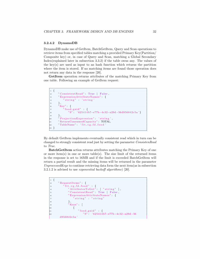
GetItem operation returns attributes of the matching Primary Key fromone table. Following an example of GetItem request:
1 {2 ”ConsistentRead” : True | False ,3 ”Express ionAttr ibuteNames ” : {4 ” s t r i n g ” : ’ s t r i n g ’5 } ,6 ”Key” : {7 ” food gu id ” : {8 ”S” : ’ 625414b7−e77b−4c32−a29d−56d956842c5a ’ }9 } ,
10 ” Pro j e c t i onExpre s s i on ” : ’ s t r i n g ’ ,11 ”ReturnConsumedCapacity” : TOTAL,12 ”TableName” : ’ f i t v g f d f o o d ’13 }
By default GetItem implements eventually consistent read which in turn can bechanged to strongly consistent read just by setting the parameter ConsistenReadto True.
BatchGetItem action returns attributes matching the Primary Key of oneor more item(s) in one or more table(s). The size limit of the returned itemsin the response is set to 16MB and if the limit is exceeded BatchGetItem willreturn a partial result and the missing items will be returned in the parameterUnprocessedKeys to continue retrieving data form the next item(as in subsection3.2.1.2 is advised to use exponential backoff algorithms) [20].
1 {2 ”RequestItems” : {3 ” f i t v g f d f o o d ” : {4 ”AttributesToGet ” : [ ” s t r i n g ” ] ,5 ”ConsistentRead” : True | False ,6 ”Express ionAttr ibuteNames ” : {7 ” s t r i n g ” : ” s t r i n g ”8 } ,9 ”Keys” : [
10 {11 ” food gu id ” : {12 ”S” : ’ 625414b7−e77b−4c32−a29d−56
d956842c5a ’

CHAPTER 3. FRAMEWORK DESIGN AND DB ENGINES 33
13 }14 }15 ] ,16 ” Pro j e c t i onExpre s s i on ” : ’ s t r i n g ’17 }18 } ,19 ”ReturnConsumedCapacity” : TOTAL20 }
BatchGetItem will return a ProvisionedThroughputExceededException if the Pro-visioned throughput is not enough to process even one item [20].
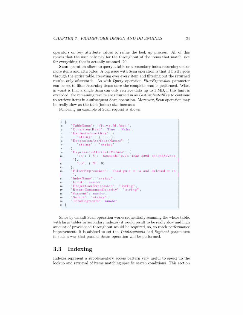
Query uses partition key to access data of a table, a local secondary index,or a global secondary index and return a result set. Specific values of thepartition key can be specified in the parameter KeyConditionExpression toallow the Query operation to return all the matching items. Resulting itemsare always returned in ascending order by the sort key value(Number of UTF-8 bytes). To filter the results, FilterExpression can be applied to determineexactly which items from the resulting ones(after Query has been executed)should be actually returned to the user [20]. If the limit of 1MB on querieditems is exceeded, the missing items might be retrieved in subsequent queryoperations starting from LastEvaluatedKey but in this case the result set mightbe required to be paginated [22]. Following an example of a Query request:
1 {2 ”ConsistentRead” : True | False ,3 ”Exclus iveStartKey ” : {4 ” s t r i n g ” : { . . . }5 } ,6 ”Express ionAttr ibuteNames ” : {7 ” s t r i n g ” : ” s t r i n g ”8 } ,9 ”KeyCondit ionExpress ion ” : ” food gu id = : a and
de l e t ed = : b” ,10 ”Expres s ionAttr ibuteValues ” : {11 ” : a” : { ’ S ’ : ’ 625414b7−e77b−4c32−a29d−56d956842c5a
’ } ,12 ” : b” : { ’N ’ : 0}13 } ,14 ” F i l t e rExp r e s s i on ” : ” s t r i n g ” ,15 ”IndexName” : ” s t r i n g ” ,16 ”Limit ” : number ,17 ” Pro j e c t i onExpre s s i on ” : ” s t r i n g ” ,18 ”ReturnConsumedCapacity” : ” s t r i n g ” ,19 ”ScanIndexForward” : boolean ,20 ” S e l e c t ” : ” s t r i n g ” ,21 ”TableName” : ’ f i t v g f d f o o d ’22 }
Query operation only operates on matching records(not the entire table) withprimary key attribute values eventually supporting a collection of comparison
CHAPTER 3. FRAMEWORK DESIGN AND DB ENGINES 34
operators on key attribute values to refine the look up process. All of thismeans that the user only pay for the throughput of the items that match, notfor everything that is actually scanned [20].
Scan operation allows to query a table or a secondary index returning one ormore items and attributes. A big issue with Scan operation is that it firstly goesthrough the entire table, iterating over every item and filtering out the returnedresults only afterwards. As with Query operation FlterExpression parametercan be set to filter returning items once the complete scan is performed. Whatis worst is that a single Scan can only retrieve data up to 1 MB, if this limit isexceeded, the remaining results are returned in as LastEvaluatedKey to continueto retrieve items in a subsequent Scan operation. Moreover, Scan operation maybe really slow as the table(index) size increases
Following an example of Scan request is shown:
1 {2 ”TableName” : ’ f i t v g f d f o o d ’ ,3 ”ConsistentRead” : True | False ,4 ”Exclus iveStartKey ” : {5 ” s t r i n g ” : { . . . } ,6 ”Express ionAttr ibuteNames ” : {7 ” s t r i n g ” : ” s t r i n g ”8 } ,9 ”Expres s ionAttr ibuteValues ” : {
10 ” : a” : { ’ S ’ : ’ 625414b7−e77b−4c32−a29d−56d956842c5a’ } ,
11 ” : b” : { ’N ’ : 0}12 } ,13 ” F i l t e rExp r e s s i on ” : ’ f ood gu id = : a and de l e t ed = : b
’ ,14 ”IndexName” : ” s t r i n g ” ,15 ”Limit ” : number ,16 ” Pro j e c t i onExpre s s i on ” : ” s t r i n g ” ,17 ”ReturnConsumedCapacity” : ” s t r i n g ” ,18 ”Segment” : number ,19 ” S e l e c t ” : ” s t r i n g ” ,20 ”TotalSegments ” : number21 }
Since by default Scan operation works sequentially scanning the whole table,with large tables(or secondary indexes) it would result to be really slow and highamount of provisioned throughput would be required, so, to reach performanceimprovements it is advised to set the TotalSegments and Segment parametersin such a way that parallel Scans operation will be performed.
3.3 Indexing
Indexes represent a supplementary access pattern very useful to speed up thelookup and retrieval of items matching specific search conditions. This section
CHAPTER 3. FRAMEWORK DESIGN AND DB ENGINES 35
aims to provide a brief presentation of the type of indexes used in MariaDB andin DynamoDB.
3.3.1 MariaDB
Indexes are used to improve lookup times in retrieving specific information morefrequently than others. They’re usually tree-based, so that looking up a certainrow via an index takes O(log(n)) time rather than scanning through the fulltable.
However, there could be drawbacks if unnecessary indexes are added makingINSERT, DELETE and UPDATE operations slower than the usual since themore indexes a table maintains the more extra information for each indexedcolumn MariaDB needs to store. By definition, it is known that any column ina large table that is frequently used in ORDER BY, WHERE and especiallyJOIN operation should have an index [32].
Imagine a table with no indexes at all. During a lookup towards one or moreattribute(s) the DB engine will start from the first row reading sequentiallythrough the whole table to reach the matched rows. The inconvenient here isthat the larger is the table, the higher is the cost in time and money. With thepresence of an index regarding the desired column(s), object of the lookup, theDB engine might rapidly find the position to explore in the middle of the datafile without to browse all the data [32].
However, if the table is small or the queries are performed on big tablesthat return most or all the rows then indexes are not a plus because sequentialreads minimize disk seeks, so, in such cases sequential lookups result faster thanworking through an index [32].
3.3.2 DynamoDB
Indexes are available also in DynamoDB under the name of Secondary Indexesand with the form of ”alternate key” to query data in a table in addition toperform queries towards the primary key. It offers two types of indexes:
• Local Secondary Indexes(LSI) allow the user to create up to 5 differentsort keys(range attributes) besides the existing Partition Key(that has toremain the same as the one created in the table). They must be createdwithin the creation of the table and once created they cannot be deleted oredited anymore. LSIs support eventual consistency as strong consistencyand basically they consume provisioned throughput from the base table inthe case of read operation while they consume two write capacity units(onefor the table and one for the index) for each of the write operations(update,delete, insert). Last but not the least LSI also allow to ”retrieve attributesthat are not projected to the index” at the price of higher latency andprovisioned throughput costs [21].
• Global Secondary Indexes(GSI) represent a new paradigm allowing theuser to create up to 5 completely new primary keys(hash key and range

CHAPTER 3. FRAMEWORK DESIGN AND DB ENGINES 36
key) each one with its own provisioned throughput. GSI might be createdwhenever the user needs and once they are created they can be edited anddeleted at any time. However, they only support eventual consistency andthey can only retrieve attributes projected to the index.
3.4 Join operations
JOIN is a fundamental relational algebra operator widely used in relationaldatabases to retrieve data from multiple tables combining matching tuplesamong the involved relations [26]. As it is well known, most of (if not all)the NoSQL database do not support this operation, not being born as rela-tional database and not having a schema, most of them neither really needit. DynamoDB does not support JOIN operations indeed and since, as otherNoSQL databases, is born to deal with the increase of data, with big tables itwould be better to avoid JOINs because the latency overhead of an individualkey lookup would somewhat large by the reason that the database would needto discover firstly towards which node(s) make the query, then make the queryitself and finally wait for the response(in most of the cases, this process wouldcreate a huge amount of foreign keys lookups through many different nodes).Moreover, if the application needs to perform large amount of JOIN operationmay be worth to denormalize2 the data. It is a common use in NoSQL databasesto have redundant data in different places to make lookups easier and faster.Moreover, most of non relational databases do not support secondary indexeseither meaning that duplicated stuff is strictly required if the application needsto make queries by other criterion.
DynamoDB should maintain denormalized data, same keys could even bestored across multiple tables but NoSQL DBs will not synchronize them auto-matically and they will not have any foreign-key meaning, even if they exists,they will be technically considered as a different set than ones in other tables andit would only be a task of the application itself to perform such synchronization.Having said that, in most of the cases for a NoSQL database like DynamoDBhaving normalized or denormalized data depends on the application use cases.
On the one hand, data could be normalized if:
• every item stored exceed the limit of 400KB and every item could be storedin different tables or in Amazon S33.
• the application needs to perform a lot of writes/updates and persistentwrites of/on item(s) larger than 1KB will impact the amount of writecapacity units(that have 1KB limit per item size) even if only one attributeis edited the WCUs considered will be the one of the entire item.
On the other hand, data’s normalization could be useful if:
2Denormaliation is a strategy used to improve lookups in a database by having redun-dant(or grouped) data and loosing something in write performance [26].
3https://aws.amazon.com/documentation/s3/
CHAPTER 3. FRAMEWORK DESIGN AND DB ENGINES 37
• items to be stored have small size and it should maintain just a few at-tributes. For reads operation an item should be equal or smaller than4KB, to not exceed the fixed limit of read capacity units while for writethe limit is 1KB.
• the application has high-traffic and consistency as data synchronizationamong tables is not its main concern.
3.5 Highlights
Besides the issue about Joins that are of course impossible and so complexdata relations have to be managed on the code/cache layer, the first thing tocome to an hand is the fact that querying data in DynamoDB is extremelylimited especially in the need to query non-indexed data. Indeed queries canbe only performed towards a single hash, on a hash/range key, or an indexand only up to 5 secondary global indexes can be created. Moreover, when itcomes to anything beyond the most basic key/value queries, DynamoDB looksstill a bit crippled. While in MariaDB, besides being possible to make queriestowards any attributes in the table, there are no specific limits on the numberof indexes(single or composite) to be created. Mainly indexes in DynamoDBare not built to speed up tables’ lookups rather to query the table towardsattributes different from the original primary key specified at the table creationstep. Another aspect which comes up from the data models is the difference innumber of supported data types between the two databases. For sure it will benecessary to parse some attributes values to build unfailing queries.
All these aspects have to be taken into account during the framework designwhere all the system is set up, the tables are created and the queries are builtto perform the benchmarking analysis.

Chapter 4
Benchmarking FrameworkImplementation
To perform our benchmarking analysis towards Amazon RDS and Amazon Dy-namoDB, a full scale testing on both online versions where required. Amazonalso provides a local version of DynamoDB but it mainly has been developedas a sort of ”getting to know” to help developers in getting familiarity with theAmazon NoSQL DB. Moreover, getting in contact with DynamoDB’s develop-ers, also them have advised not to perform analysis on local version since theresults may fluctuate drastically.
Figure 4.1: Example of a simple AWS application structure
AWS applications, in general, involve a lot of different components interact-ing among them, setting up connections, exchanging messages and informations.To avoid any traffic interaction time in our analysis the main idea was to logall the benchmarking analysis at database level so that the real query time(andonly that) could be monitored and recorded. Although this could have beeneasily done with RDS, DynamoDB does not support any kind of database levellogging and due to this, the plan has been deviated in favour of the API level.In order to do that, and to deal with some issues such as DB caching, TCPtimes, connection times, authentication (and so on) a proper framework hasbeen implemented.
38

CHAPTER 4. BENCHMARKING FRAMEWORK IMPLEMENTATION 39
Fig. 4.1 shows a really simplified AWS application structure and the ex-tracted components used in this work. The API is maintained in the EC2 in-stance and it is directly connected to both Amazon RDS instance and AmazonDynamoDB. All of this happens within a private subnet availability zone.
As it has already been explained in the previous chapter, since most of theuseful operations from relational databases, such as JOIN, AVG, MIN, MAX arenot supported by DynamoDB (and NoSQL DBs in general), the benchmarkinganalysis framework on this work has been built essentially on five basic oper-ations to be performed, that are Read, Write(Insert and Update), Delete andQuery on Indexes.
All the queries shown in subsections 4.2.2 and 4.2.3 have been performedacross all the tables involved in both databases retrieving, updating and deletingitems through their Primary Key/Indexes or inserting by providing a Foodobject built through the Factories5. The time recorded from every API callsis the time that starts when the query is issued until a valid response is returnedback by the database.
4.1 Caching
Amazon RDS makes use of database caching which allows to store results ofSELECT queries so that if an identical query is received in future, the resultscan be quickly returned. In order to avoid that, for a fair comparison, cachinghad to be disabled in both databases. Connecting to the RDS instance it ispretty simple to check whether the query cache is available and enabled, by justrunning the following query:
SHOW VARIABLES LIKE ’have_query_cache’;
+------------------+-------+
| Variable_name | Value |
+------------------+-------+
| have_query_cache | YES |
+------------------+-------+
If the query returns YES as in the result above, then the query cache is available.To disabled it, it is enough just to set a couple of variables to 0. This has beendone by running:
set global query_cache_type=0;
set global query_cache_size=0;
flush query cache;
reset query cache;
From now on, the RDS cache is disabled so every query can be run fairly un-der this point of view. From the AWS documentation and AWS support, Dy-namoDB does not provide any caching service.
5http://factoryboy.readthedocs.io/en/latest/orms.html

CHAPTER 4. BENCHMARKING FRAMEWORK IMPLEMENTATION 40
4.2 API level(Django Framework)
Django framework has been chosen as high-level Python Web framework since itis free of charge, open source, it is provided by a really complete documentationand it takes care of many concerns about Web development. This frameworkalso allows the developers to create custom fully integrated commands to beexecuted from the instance’s terminal and for the purpose of this work thisfeature was perfect since it was possible to create a command to be run for eachof the operation involved in the benchmarking analysis.
Django provides an official backend1 for relational databases to take careabout setup and connections while it provides models to allow any interactionbetween the application and the database instance. However, Django does notprovide any implemented backend for NoSQL DBs and unfortunately to build anentire backend from the scratch would have meant to rewrite the whole DjangoORM which takes a huge amount of work, time and effort.
Playing around the inconvenient, luckily Amazon released an interestingSDK for Python called boto3 which allows to get the connection to DynamoDBand to perform operations on it. ”Boto is the Amazon Web Services (AWS) SDKfor Python that provides an easy to use, object-oriented API as well as low-leveldirect service access” [19].
4.2.1 Operation’s definitions
All the operations taken into account in this work are defined as follow:
? Reads.
– Read the value corresponding to a given key. This is the same asthe read operation in the CRUD model.
– Read the value/values corresponding to a non-key(index or generalattribute)
? Write.
– Save a new item in the table. This represents the same as the insertoperation in the CRUD model.
– If a given key-value pair is not found in the table, then the item isadded to the table. Otherwise, it updates the value for the givenkey. This operation combines Create and Update operations of theCRUD model.
? Update.
1Django provides some basic well-documented implementations of authentication, caching,database setup, setting variables (and so on) to anticipate the need of adding own custom”backend” implementation and own custom modules.

CHAPTER 4. BENCHMARKING FRAMEWORK IMPLEMENTATION 41
– Update an item in the table. This is the same as the update opera-tion in the CRUD model.
– If a given key-value pair is found, then it updates the provided valuefor the given key.
? Delete.
– Delete the record corresponding to given primary key. This is thesame as the delete operation in the CRUD model.
– If the key is not found, then an empty response is returned.
? Read by Index. Retrieve one or more item(s) corresponding to a givenindex value. This could be thought as the same as the read operation inthe CRUD model but by providing an index instead of a primary key.
? Read by Index with Conditions. Retrieve one or more item(s) corre-sponding to the given index value and matching a specified condition.
Besides these queries to evaluate scalability and performance on items’ requestsalso throttling, errors and Global Secondary Index creation have been treatedand monitored.
The query time of each operation was simply recorded through a straight-forward Python module called time2 [38]. The following lines of code show theactual calculation of the query time used throughout the benchmarking analysis:
1 l i s tQueryTimes = [ ]2 t = time . time ( )3 ”””QUERY TO BE PERFORMED”””4 newTime = ( time . time ( ) − t ) ∗ 10005 l i s tQueryTimes . append (newTime)
Although the time is returned as floating point value, not all the system canassure better precision of 1 second so, as workaround of possible issues, the timehas been always recorded in milliseconds by simply multiplying per 1000 thedifference between the start and stop values returned from time function.
4.2.2 Django models
In a Django web application, data is accessed and managed through Pythonobjects known under the name of models. Django models map to databasetables defining the structure of the stored data, including field types, sizes, de-fault values, etc. and providing an ”environment” to encapsulate business logic.This helps developers to have a more structured logic without having to dealwith long complex queries built in plain SQL. Once a database engine is chosen
2time.time() returns the time in seconds since the epoch as a floating point number. Eventhough the time is always returned as a floating point number, not all systems provide timewith a better precision than 1 second.

CHAPTER 4. BENCHMARKING FRAMEWORK IMPLEMENTATION 42
and settled, Django takes care about all the communications and transactionsand developers can concentrate their efforts in building the application makingall the queries through the database-abstraction API provided by Django.
For the purpose of our analysis a model to map the table fit vg fd food(objectof this work) has been created as class FoodBase(models.Model). The namebase has been given because the model is actually a base to create all the otherneeded tables in such a way they are all equals but with different sizes.
Once models are created, to let Django the use of them, it is enough to setthe INSTALLED APPS parameter by adding the name of the module whichcontains the created models.
Django uses the class QuerySet3 to create queries towards its models:
1 c l a s s QuerySet (model=None , query=None , us ing=None ) [source ]
Most of these QuerySets return other QuerySet objects allowing to chain refine-ments together in order to perform a sort of complex nested queries.
The operations defined in subsection 4.2.1, in Django are performed as fol-lows:
4.2.2.1 Write
Both the following insert operations come from the description in subsection3.2.1.1:
• Insert a single item. Django uses the class Model(**kwargs) [36] tobuild the object and the keyword arguments are simply the names of thefields(attributes) defined in the Food model.
1 Food (∗∗ food ) . save ( )
In this case the keyword argument **food represents a dictionary contain-ing keys and values of the item that has to be saved in the table. Themethod save() eventually performs the operation to insert the built objectin the table.
• Insert batch of items Objects are saved in batch through the QuerySetbulk create(objs, batch size=None) [36]. The list objs may contain”any” number of items to be inserted in the table and in the case of thiswork is expressed by rdsBulkList :
1 Food . ob j e c t s . bu l k c r e a t e ( rdsBulkL i s t [ index : index + 25 ] )
To have a fair comparison has been decided to limit the batch at 25 ele-ments since DynamoDB has this limit with batch write item operation.
3https://docs.djangoproject.com/en/1.11/ref/models/querysets/

CHAPTER 4. BENCHMARKING FRAMEWORK IMPLEMENTATION 43
4.2.2.2 Update
Firstly the item(s) to be updated are filtered by primary key through the Query-Set filter(**kwargs) and it returns the QuerySet containing objects matchingthe given lookup parameters [36].
1 Food . ob j e c t s . f i l t e r ( guid=guid )2 . update ( f o o d u r l i d=’ apples−raw−with−sk in ’ )
As in subsection 3.2.2.1 objects are updated through the QuerySet update(**kwargs)[36] where kwargs contains the attribute(s) to be updated.
4.2.2.3 Delete
As in subsection 3.2.3.1, objects are deleted through the QuerySet delete() [36].The item(s) to be deleted are firstly selected through the QuerySet filter.
1 Food . ob j e c t s . f i l t e r ( guid=keys [ i ] , d e l e t ed=0 ) . d e l e t e ( )
With Foreign keys Django adopts ON DELETE CASCADE feature deletingalso any object pointing at the objects to be deleted.
4.2.2.4 Read
As in subsection 3.2.4.1, objects are retrieved from the database through theQuerySet get(**kwargs) [36]. The following primary key
1 key = {2 ’ f ood gu id ’ : { ’ S ’ : ’ 871 af1c4−1e32−4278−91ab−0a31ae83abc8 ’ } ,3 ’ d e l e t ed ’ : { ’N ’ : 0 }4 }
is given. In this query the keyword arguments are represented by only thecomposite primary key (guid, deleted):
1 Food . ob j e c t s . get ( guid=key [ ’ f ood gu id ’ ] [ ’ S ’ ] , d e l e t ed=0 )
4.2.2.5 Operation on indexes
• Query on index. Objects are retrieved from the database with theQuerySet get(**kwargs) where the keyword arguments are representedby a single index attribute:
1 Food . ob j e c t s . f i l t e r ( user = 3 )
• Query on index with conditions. Objects are retrieved from the databasethrough the Query Related tool class Q[source]. Q() objects allow thecreation of complex query with conditions:
1 Food . ob j e c t s . f i l t e r ( Q( user=3) &2 Q( f o o d t y p e l t e =3, f o od t yp e g t e=1) &3 Q( de l e t ed=0) )

CHAPTER 4. BENCHMARKING FRAMEWORK IMPLEMENTATION 44
The previous query is in charge to retrieve all the food items matchingthe following combinations:
1 u s e r i d = 3 , 1 < f ood type < 3 and de l e t ed = 0
4.2.3 Boto 3 SDK for DynamoDB
While, in Django framework, provided models have been used, in DynamoDBa wrapper class called DynamoDBManager has been created to deal withthe connection and to collect all the operations required to perform our bench-marking analysis properly allowing to easily manage all the boto3 calls in everyscript. Boto 3 provides a resource or a low level low-level client to representAmazon DynamoDB and operates on the tables. For this work client has beenchosen to have better performance benchmarking since resource keeps trying toquery if the operation does not succeed straight away while client returns anerror.
1 c l a s s DynamoDBManager :2 de f i n i t ( s e l f , table name ) :3 s e l f . dynamo=boto3 . c l i e n t ( ’dynamodb ’ , region name=’ eu−west−1 ’ )4 s e l f . t ab l e=table name5
6 de f i n s e r t ( s e l f , item ) : . . .7
8 de f i n s e r t b a t c h ( s e l f , item ) : . . .9
10 de f de l e t e i t em by key ( s e l f , key ) : . . .11
12 de f d e l e t e ba t ch ( s e l f , keys ) : . . .13
14 de f update ( s e l f , key , update expres s ion , e xp r e s s i o n va l u e s ) : . . .15
16 de f ge t i t em ( s e l f , key ) : . . .17
18 de f batch ge t i t em ( s e l f , key ) : . . .19
20 de f query ( s e l f , key cond i t ion , e xp r e s s i on va l u e ) : . . .21
22 de f query by index ( s e l f , index , key cond i t ion , e xp r e s s i on va l u e ) :. . .
23
24 de f que ry index cond i t i on ( s e l f , index , key cond i t i on ,exp r e s s i on va lu e s , f i l t e r e x p r e s s i o n ) : . . .
25
26 de f scan ( s e l f , f i l t e r e x p r e s s i o n , e xp r e s s i on va l u e ) : . . .
The DynamoDBManager class makes use of the class DynamoDB.Client as alow-level client representing Amazon DynamoDB and a table name. To createan object with DynamoDBManager an existing table name has to be provided.Once the object is created it can make use of all the methods provided by the

CHAPTER 4. BENCHMARKING FRAMEWORK IMPLEMENTATION 45
DynamoDB.Client(some of them, the ones used in this work, are provided inthe class as methods of the object itself)4. Following all the operations used inthis work are presented.
4.2.3.1 Write
Both the following insert operations come from the description in Subsection3.2.1.2:
• Insert a single element with the method put item(**kwargs). Keywordarguments are represented by the table name and the item to be insertedin the form exposed in fig. 4.3.
1 re sponse = s e l f . dynamo . put item (2 TableName=s e l f . tab le ,3 Item=item4 )
• Insert a batch of 25 items with the method batch write item(**kwargs).Keyword arguments are represented by the table name and a list of itemseach one in a dictionary shape as shown in fig. 4.3.
1 re sponse = s e l f . dynamo . ba t ch wr i t e i t em (2 RequestItems={3 s e l f . t ab l e : i tems4 }5 )
4.2.3.2 Update
The update operation makes use of the method update item(**kwargs) largelydiscussed in Subsection 4.2.3.2(3.2.2)
1 re sponse = c l i e n t . update item (2 TableName=s e l f . tab le ,3 Key={4 ’ f ood gu id ’ : { ’ S ’ : s t r ( guid ) } ,5 ’ d e l e t ed ’ : { ’N ’ : 0}6 } ,7 UpdateExpression=” s e t f o o d u r l i d = : t ” ,8 Expres s ionAttr ibuteVa lues={9 ’ : t ’ : { ’ S ’ : s t r ( ’ apples−raw−with−sk in ’ ) }
10 } ,11 ReturnValues=”UPDATEDNEW”12 )
The keyword arguments passed to the method is made by five parameters: thetable name, the primary key needed to specify the item to be updated, a state-ment containing the attribute name to be updated, the new value to be setin the specified attribute and a parameter ReturnValues that has been set toUPDATED NEW to return the updated items in the response(useful to checkif the query has been executed properly).
4http://boto3.readthedocs.io/en/latest/reference/services/dynamodb.html

CHAPTER 4. BENCHMARKING FRAMEWORK IMPLEMENTATION 46
4.2.3.3 Delete
Both the following delete operations come from the description in subsection3.2.3.2
• delete item(**kwargs) method is used by DynamoDB to perform thedeletion operation of a single item. It takes as keyword arguments thetable name and the primary key of the item to be deleted.
1 re sponse = s e l f . dynamo . d e l e t e i t em (2 TableName=s e l f . tab le ,3 Key={ ’ f ood gu id ’ : { ’ S ’ : s t r ( guid ) } ,4 ’ d e l e t ed ’ : { ’N ’ : 0 } }5 )
• batch write item(**kwargs) is method used by DynamoDB to deletebatch of items. It takes as keyword arguments the name of the table anda list of primary keys to be deleted from such table.
1 i tems = [ ]2 f o r i in range ( l en ( keys ) ) :3 i tems . append ({4 ’ DeleteRequest ’ : {5 ’Key ’ : { ’ f ood gu id ’ : { ’ S ’ : keys [ i ] } ,6 ’ d e l e t ed ’ : { ’N ’ : 0 } }7 }8 })9 t = time . time ( )
10 re sponse = s e l f . dynamo . ba t ch wr i t e i t em (11 RequestItems={ s e l f . t ab l e : i tems }12 )
4.2.3.4 Read
As presented in subsection 3.2.4.2 DynamoDB owns four methods to retrieveitems from the tables. The following primary key was provided:
1 key = {2 ’ f ood gu id ’ : { ’ S ’ : ’ 871 af1c4−1e32−4278−91ab−0a31ae83abc8 ’ } ,3 ’ d e l e t ed ’ : { ’N ’ : 0 }4 }
• DynamoDB retrieves item(s) corresponding to a given primary key throughthe method get item(**kwargs), which takes as arguments such pri-mary key and the table name.
1 re sponse = s e l f . dynamo . ge t i t em (2 TableName=s e l f . tab le ,3 Key=key ,4 ConsistentRead=True5 )
The parameter ConsistentRead has been set to True to have stronglyconsistent reads and so to read from an updated table.

CHAPTER 4. BENCHMARKING FRAMEWORK IMPLEMENTATION 47
• To return attributes from one or more items in one or more tables Dy-namoDB uses the method batch get item(**kwargs). Same line ofget item() but with a list of keys passed as parameter.
1 re sponse = s e l f . dynamo . batch ge t i t em (2 RequestItems={3 s e l f . t ab l e : { ’ Keys ’ : [ key ] }4 }5 )
• To access items of a the table through either a primary key or indexDynamoDB uses the method query(**kwargs). Keyword arguments arethe table name, the key conditions and the required values to compute thecondition expression.
1 re sponse = response = s e l f . dynamo . query (2 TableName=s e l f . tab le ,3 KeyCondit ionExpress ion=’ food gu id = : a AND de l e t ed = : b ’ ,4 Expres s ionAttr ibuteVa lues={ ” : a” : key [ ’ f ood gu id ’ ] ,5 ” : b” : key [ ’ d e l e t ed ’ ] }6 )
• scan(**kwargs) represent a really expensive operation that could alsobe used to retrieve items from a table but it first accesses every item insuch table(or secondary index). As query operations, the keyword argu-ments are the table name, the key conditions and values for the conditionexpression.
1 re sponse = s e l f . dynamo . scan (2 TableName=s e l f . tab le ,3 F i l t e rExp r e s s i on=’ food gu id = : a and de l e t ed = : b ’ ,4 Expres s ionAttr ibuteVa lues={ ” : a” : key [ ’ f ood gu id ’ ] ,5 ” : b” : key [ ’ d e l e t ed ’ ] }6 )
4.2.3.5 Operation on indexes
To query items by index(GSI different attribute from the primary key) has beendecided to use query(**kwargs) because scan operation required too high readcapacity units and it anyway took a really high query time.
• By only index.
1 re sponse = s e l f . dynamo . query (2 TableName=s e l f . tab le ,3 IndexName=’ us e r id−index ’ ,4 KeyCondit ionExpress ion=’ u s e r i d = : u ’ ,5 Expres s ionAttr ibuteVa lues={ ” : u” : { ’N ’ : s t r (3 ) } }6 )
The keyword args are the table name, the index name, the key conditionrepresented by the index and the value for the condition expression.

CHAPTER 4. BENCHMARKING FRAMEWORK IMPLEMENTATION 48
• By index with conditions.
1 re sponse = s e l f . dynamo . query (2 TableName=s e l f . tab le ,3 IndexName=’ us e r id−index ’ ,4 KeyCondit ionExpress ion=’ u s e r i d = : u ’ ,5 Expres s ionAttr ibuteVa lues={ ’ : u ’ : { ’N ’ : s t r (3 ) } ,6 ’ : g ’ : { ’N ’ : s t r (1 ) } ,7 ’ : l ’ : { ’N ’ : s t r (3 ) } ,8 ’ : d ’ : { ’N ’ : s t r (0 ) }9 } ,
10 F i l t e rExp r e s s i on=’ food type BETWEEN : g and : l AND de l e t ed=:d’
11 )
The keyword args are the table name, the index name, the key conditionexpression, a dictionary for the expression attributes values and the filterexpression for such values.
4.2.4 Database Tables
In each database have been created four tables of different sizes, respectively100 thousands, 1 million, 10 millions and 75 million items. For the purposeof these analysis has been decided to populate all of the tables with the samedata migrated in parallel from a real table, fit vg fd food, containing real datafrom the cloud. To migrate data in parallel has been used a multiprocessingenvironment with 8 CPUs and 32GB of RAM. Every process was in charge tomigrate around 50 thousands of items(each one of about 1KB in size) at timenot to bubble over the DyanamoDB write capacity units that have been set to5000 in all the tables to speed up the process. Further description and details ofthe migration process are out of the purpose of this work. The following tableshows the final setup of the tables with their final size and number of items:
Table Name Table Size Number of itemsfit vg fd food 71.58 GB ∼ 75 millionsfood 100 ths 111.90 MB ∼ 115 thousandsfood 1 mln 966.64 MB ∼ 1 millionfood 10 mln 9.55 GB ∼ 10 millions
The tables used in Amazon MariaDB roughly reflects the one used in produc-tion with same indexes, data and settings. Tables used in Amazon DynamoDBneeded to be adjusted in matters of indexes and data types presented in sub-sections 4.2.5 and 4.2.6.
The Primary Key in all the tables have been thought to be a composite keymade by:
• a string value food guid(e.g. 0cc14119-c723-4687-9d76-80ddc4438a76)
• an integer value deleted(e.g. 0 or 1)
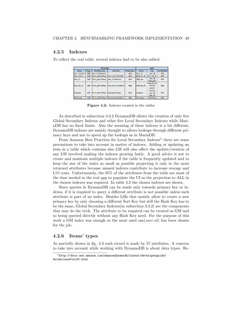
CHAPTER 4. BENCHMARKING FRAMEWORK IMPLEMENTATION 49
4.2.5 Indexes
To reflect the real table, several indexes had to be also added:
Figure 4.2: Indexes created in the tables
As described in subsection 3.3.2 DynamoDB allows the creation of only fiveGlobal Secondary Indexes and other five Local Secondary Indexes while Mari-aDB has no fixed limits. Also the meaning of these indexes is a bit different,DynamoDB indexes are mainly thought to allows lookups through different pri-mary keys and not to speed up the lookups as in MariaDB.
From Amazon Best Practices for Local Secondary Indexes1 there are someprecautions to take into account in matter of indexes. Adding or updating anitem in a table which contains also LSI will also affect the update/creation ofany LSI involved making the indexes growing fastly. A good advice is not tocreate and maintain multiple indexes if the table is frequently updated and tokeep the size of the index as small as possible projecting it only in the mostreturned attributes because unused indexes contribute to increase storage andI/O costs. Unfortunately, the 95% of the attributes from the table are most ofthe time needed in the real app to populate the UI so the projection to ALL inthe chosen indexes was required. In table 4.2 the chosen indexes are shown.
Since queries in DynamoDB can be made only towards primary key or in-dexes, if it is required to query a different attribute is not possible unless suchattribute is part of an index. Besides LSIs that mainly allow to create a newprimary key by only choosing a different Sort Key but still the Hash Key has tobe the same, Global Secondary Indexes(in subsection 3.3.2) are the componentsthat may do the trick. The attribute to be required can be created as GSI andso being queried directly without any Hash Key need. For the purpose of thiswork a GSI index was enough so the most used one(user id) has been chosenfor the job.
4.2.6 Items’ types
As partially shown in fig. 4.3 each record is made by 57 attributes. A concernto take into account while working with DynamoDB is about data types. Re-
1http://docs.aws.amazon.com/amazondynamodb/latest/developerguide/
GuidelinesForLSI.html

CHAPTER 4. BENCHMARKING FRAMEWORK IMPLEMENTATION 50
lational databases support a huge amount of data types while NoSQLs (in thiscase DynamoDB) do not.
Figure 4.3
Example of Django model(sx) and item from DynamoDB(dx)
Data types supported by DynamoDB are just a few compared with MariaDB:
• Scalar: Number, String, Binary, Boolean, and Null
• Multi-valued: String Set, Number Set, and Binary Set
• Document: List and Map
Even if less types are supported, these seem to be enough to collect all therequired data. Sometimes workaround can be found from the API level, asfor DATETIME that can be easily converted in a timestamp as integer to besaved in the database and then it could be converted back in plain date after aresponse back from the db when it is requested from the API.
4.3 DB Connection time, logic behind the schema
As it has already been said in the intro of this chapter, benchmarking analy-sis performed from the API level are affected by several components involvedin the connection process towards the DB such as the three-way handshake,authorization, authentication, etc.

CHAPTER 4. BENCHMARKING FRAMEWORK IMPLEMENTATION 51
Figure 4.4: APP - DBs transactions
Being conscious to what extent these values can interfere with the actualquery time it is fundamental. To measure the connection time it has beendecided to run a million times a very simple query(select) towards a table con-taining only one element. Doing so, the time it takes to be executed from thedatabase engine is negligible and most of the time is taken by the connectionprocess.
Throughout the project the actual time is simply taken by using a pythonmodule called time. It is called just before the query call to get the startingtimestamp λ1 and right after the same query to get the stopping timestamp λ2.Having those timestamps, the amount of time between the two is calculated witha simple subtraction getting δ(Eq. 4.1). Summing n times δ it becomes possibleto calculate its average that goes under the name of Θ(Eq. 4.2). Furthermore,to have a more refined estimation of the connection time, Θ has been computedseveral times(m) and its average has been also calculated ending up with anoverall average called Γ(Eq. 4.3). (Details of the equation below can be foundin table 4.1)
Variable Description Valuen N. of calls to the database 2000m N. of cycles 5λ1 Start time counter time.time(ms)λ2 Stop time counter time.time(ms)δ Range of time between start counter and stop λ2 − λ1Θ Sum of the timestamps from the n calls −Γ Sum of the Θ values calculated in the m cycles −
Table 4.1: Formulas’ legenda.
δ = λ2 − λ1 (4.1)
Θ =1
n
n∑i=1
δi (4.2)
Γ =1
m
m∑i=1
Θi (4.3)
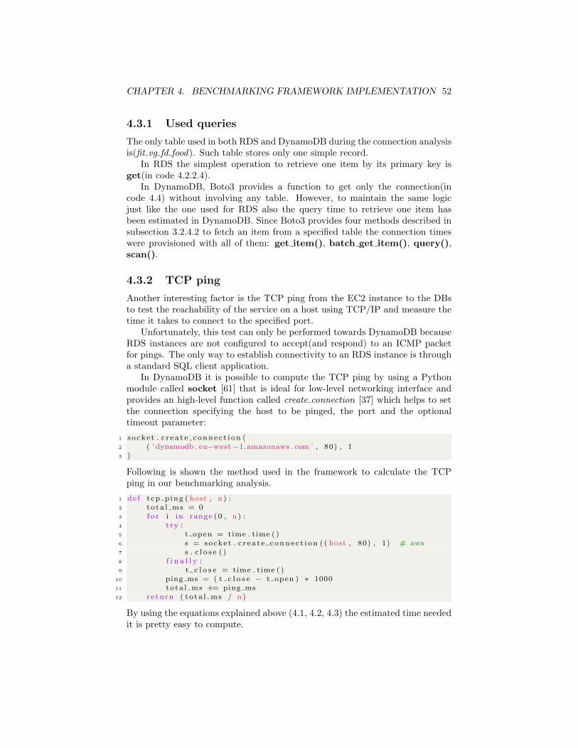
CHAPTER 4. BENCHMARKING FRAMEWORK IMPLEMENTATION 52
4.3.1 Used queries
The only table used in both RDS and DynamoDB during the connection analysisis(fit vg fd food). Such table stores only one simple record.
In RDS the simplest operation to retrieve one item by its primary key isget(in code 4.2.2.4).
In DynamoDB, Boto3 provides a function to get only the connection(incode 4.4) without involving any table. However, to maintain the same logicjust like the one used for RDS also the query time to retrieve one item hasbeen estimated in DynamoDB. Since Boto3 provides four methods described insubsection 3.2.4.2 to fetch an item from a specified table the connection timeswere provisioned with all of them: get item(), batch get item(), query(),scan().
4.3.2 TCP ping
Another interesting factor is the TCP ping from the EC2 instance to the DBsto test the reachability of the service on a host using TCP/IP and measure thetime it takes to connect to the specified port.
Unfortunately, this test can only be performed towards DynamoDB becauseRDS instances are not configured to accept(and respond) to an ICMP packetfor pings. The only way to establish connectivity to an RDS instance is througha standard SQL client application.
In DynamoDB it is possible to compute the TCP ping by using a Pythonmodule called socket [61] that is ideal for low-level networking interface andprovides an high-level function called create connection [37] which helps to setthe connection specifying the host to be pinged, the port and the optionaltimeout parameter:
1 socke t . c r e a t e c onne c t i on (2 ( ’dynamodb . eu−west−1.amazonaws . com ’ , 80) , 13 )
Following is shown the method used in the framework to calculate the TCPping in our benchmarking analysis.
1 de f t cp p ing ( host , n ) :2 to ta l ms = 03 f o r i in range (0 , n ) :4 t ry :5 t open = time . time ( )6 s = socket . c r e a t e c onne c t i on ( ( host , 80) , 1) # aws7 s . c l o s e ( )8 f i n a l l y :9 t c l o s e = time . time ( )
10 ping ms = ( t c l o s e − t open ) ∗ 100011 to ta l ms += ping ms12 r e turn ( to ta l ms / n)
By using the equations explained above (4.1, 4.2, 4.3) the estimated time neededit is pretty easy to compute.

CHAPTER 4. BENCHMARKING FRAMEWORK IMPLEMENTATION 53
4.4 Benchmarking operators
Round-trip times of requests from API level can ”bounce” up and down. This isthe reason why every query has been run for many times and every timestamphas been recorded and saved in a list. Once the list has been created threemethods have been used. To get a good approximation of the query time theaverage of the timestamp’s list has been calculated and along with this also thestandard deviation to have a precise measure of the mathematical dispersion ofthe query times from the mean.
• Mean. To calculate the average a formula from the original algorithm tocompute the weighted average of RTT in the Adaptive RetransmissionBased on Round-Trip Time [48] has been applied:
OldT imestamp = (α∗OldT imestamp)+((1−α)∗NewTimestamp) (4.4)
In the formula, α represents a smoothing factor with a value between 0and 1. Values of α closer to 1 provide a better smooth in situation wherethe query time fluctuate wildly. In contrast values of α closer to 0 makethe query time change more quickly in reaction to changes in measuredquery times. Between 0.8 and 0.9 (typically 0.875) is the ”optimal” value.
1 de f mean( t imestampList ) :2 alpha = 0.8753 n = len ( t imestampList )4 OldTimestamp = timestampList [ 0 ]5 f o r i in range (1 , n ) :6 OldTimestamp = ( alpha ∗ OldTimestamp ) + ((1 − alpha ) ∗
t imestampList [ i ] )7 r e turn OldTime
The function mean accepts a list of timestamps taken from the performedqueries as argument. Then it applies the formula in Eq.4.4 to calculatethe mean throughout the provided list.
• Variance.
σ2 =
∑nn=1(X − µ)2
n(4.5)
where µ is the mean of the query times(from Eq.4.4) and n is the totalnumber of query times recorded in each query test.
1 de f var i ance ( data , mu) :2 n = len ( data )3 i f n < 2 :4 r a i s e ValueError ( ’ va r i ance r e qu i r e s at l e a s t two data
po in t s ’ )5 v = (sum( ( x − mu) ∗∗2 f o r x in data ) ) /n6 r e turn v
• Standard Deviation. Once the mean and the variance are calculated,it is pretty easy to compute the standard deviation(σ) that is represented

CHAPTER 4. BENCHMARKING FRAMEWORK IMPLEMENTATION 54
by the square root of the variance σ2:
σ =2√σ2 (4.6)
The Standard deviation helps to understand how good are the found meansin respect to the amount of query times recorded.
1 de f s td dev ( data , mu) :2 var = var iance ( data , mu)3 r e turn math . s q r t ( var )
• DynamoDB connection. With this operation it is possible to have arough estimation of the setup time required to build the connection toAmazon DynamoDB from API level created through the client. It couldbe interesting to see if this plain connection is in line with the connectiontimes examined in subsection 4.3.
1 de f dynamo connection (db , r eg i on ) :2 t s end = time . time ( )3 boto3 . c l i e n t (db , region name=reg i on )4 r e turn ( time . time ( ) − t s end ) ∗ 1000

Chapter 5
Discussion of analysis
Unfortunately, there are no universal metrics to measure performance of key-values solutions due to their different goals and capabilities. It is clear thattrying to evaluate a database as DynamoDB, which is designed for write avail-ability above everything else, in the area of consistency, is not fair since theoverall system has been create to enforce availability above consistency.
Beside this, one of the most important concerns about web application is thetime required to complete a task. In case of a database, this factor is redirectedto the time required to complete a transaction. Analysing this time along withscalability and throughput it turned out that all these components may help toget some requirements and eventually to provide an accurate overview and deepunderstanding of the examined solutions.
The main aim of this work is to present a benchmarking analysis from therequirement of the company Virtuagym that is trying to solve the problem ofslow queries in some transactions due to the day by day increase in size of somespecific tables.
5.1 Connection measurements
From fig.5.1, the connection time to DynamoDB from the EC2 instance reacha peak at about 33.8ms in the first connection then it tends to balance toabout 1.9ms in all the other connection tests. This happen because when acommand towards DynamoDB is performed, it firstly needs to verify the AWScredential and then to make resources available for the tables to read while forevery subsequent call it will reuse those resources. Indeed, running the scriptmany times(by calling it from the Django command manage.py) it always takesaround 30ms(which is roughly the same amount of time compare with the peak),but when the call is made several times in a for loop within the same script, eachcall’s time decrease drastically until a period of no operation where Dynamoseems to close down the resources to save on it. For this reason and for thepurpose of our benchmarks analysis the very first call to DynamoDB should
55

CHAPTER 5. DISCUSSION OF ANALYSIS 56
always be discarded.The TCP ping time to DynamoDB is almost always around 0.85ms in aver-
age, meaning that DynamoDB instance is fastly reachable.
Figure 5.1
Connections times(table B.1)
Query time to get an item from an RDS instance seems to be pretty bal-anced along all the calls and cycles keeping on track at about 2.16ms whileall the query times to DynamoDB fluctuate a lot due to the many interac-tions(connections, latencies, packet exchanges) happening in the backend sideof DynamoDB. However, since DynamoDB has several methods to retrieve arecord from a table, it was interesting to check if the time every method takesto get the same item was roughly the same or extremely different. As shownin fig. 5.1, most of the times are pretty close in time, between 2ms and 7ms,apart from Scan operation that in average takes around 28ms.
5.2 Key metrics
The following table shows some of the key metrics considered throughout thebenchmarking analysis:

CHAPTER 5. DISCUSSION OF ANALYSIS 57
Name DescriptionSuccessful RequestLatency
Response time (in ms) of successful requests inthe selected time period to metric the perfor-mance. Also can report an estimated numberof successful requests (data samples).
Provisioned ReadCapacity Units
Number of read capacity units you provisionedfor a table (or a global secondary index) dur-ing the selected time period .
Provisioned WriteCapacity Units
Number of write capacity units you provi-sioned for a table (or a global secondary index)during the selected time period .
5.3 Speed and throughput
One of the most popular metrics to measure database performance is the speedto perform a full transaction taking into account its throughput, that involvesthe number of completed transactions in a unit of time. For each pf the followingbar charts, the tables showing the exact results are provided in appendix B whilethe errors charts to check the Standard Deviation is provided in appendix A.
The following benchmarks were performed for read operations setting readunits to 200. In DynamoDB Query operation is expected to be very fast andonly slightly slower than Get operation. The scan operation on the other handmay take anywhere from few milliseconds to a few hours to complete dependingon the size of the table because it is performed by going through each item inthe table. For any reasonably sized table the scan operation will consume allthe provisioned read units until the operation finishes. Indeed, in fig. 5.2 Scanoperation is the one that takes most to execute the fetching of the data.
Figure 5.2
Read operations with Dynamo Scan (table B.6)
To have a better overview of the query times, in fig.5.3 it has been decided

CHAPTER 5. DISCUSSION OF ANALYSIS 58
to get rid of Scan operation and shows only the others. It was expected tosee DynamoDB being faster than MariaDB in retrieving data, especially withthe growth of the tables’ sizes. As it is clear, RDS Get is faster on the overalltest ranging between 2.26 and 2.86 ms compared with any of the DynamoDB’squeries. Query operations results stable overall and mostly faster than bothGetItem and BatchGet which seem to perform better with large size tablesthan smaller ones.
Figure 5.3
Read operations without Dynamo Scan(table B.5)
Write benchmarks described in subsections 4.2.2.1 and 4.2.3.1 with 500writes units are shown in fig.5.4. Against every expectation the overall writeoperations run from DynamoDB turns out to be faster than the RDS coun-terpart. DynamoDB PutItem results faster than SaveRDS which takes morethan double of the time to retrieve one item. DynamoDB BatchWrite with arange of 33 to 37 ms still performs faster inserts with batch of 25 items thanRDS BulkCreate that takes from 84ms in the smallest table up to 115ms inthe biggest one. This test also shows the scalability performed on PutItem byDynamoDB while other operations seem to be affected by the increase in sizeof the table.

CHAPTER 5. DISCUSSION OF ANALYSIS 59
Figure 5.4
Write operations(table B.2)
Fig.5.5 shows the comparison between two updates operations described insubsections 4.2.2.2 and 4.2.3.2. Both write and read capacity units were setto 100. Throughout the test all the update operations made by RDS remainbalanced around 4ms and faster than DynamoDB update operations that arealso pretty balanced around 5ms with a peak of almost 6ms in the 75millionsitems table.
Figure 5.5
Update operations(table B.3)
As shown in fig.5.6 delete one item from RDS MariaDB employs on averagearound 4ms resulting slightly faster than DynamoDB. DeleteItemDynamo(code4.2.3.3) seems to be affected by the increasing table size, indeed, it takes around5ms towards the 100thousands table ms and the query times rises up to around6ms for the item’s deletion from the biggest table of 75millions items. Besidessingle item’s deletion, a 25 items’ deletion from their primary keys was testedin DynamoDB while MariaDB does not own any query to delete more keys in

CHAPTER 5. DISCUSSION OF ANALYSIS 60
parallel. BatchDeleteDynamo has a peak at 8.44ms in the smaller table whilethe query time seems to balance at around 5ms in the other tables being evenfaster than RDS in the table with 10millions items. All the delete operationsfrom DynamoDB had read capacity units set to 100.
Figure 5.6
Delete operations(table B.4)
Fig. 5.7 shows the query times to retrieve items matching a provided indexkey-value(in code 4.2.3.5 and 4.2.2.5) while fig. 5.8 shows query times to fetchitems by providing index key-value and conditions(in code 4.2.3.5 and 4.2.2.5).Both operations from DynamoDB had read capacity units set to 100. The resultsfrom both the tests look pretty similar meaning that with this implementation,querying a table towards an index with or without conditions does not affectthe query time too much. However, the difference in time among the opera-tion from RDS and DynamoDB in both the test is embarrassedly huge withRDS constantly standing between 0.28 and 0.42 milliseconds while DynamoDBranging between roughly 900 and 921 milliseconds in fig. 5.7.
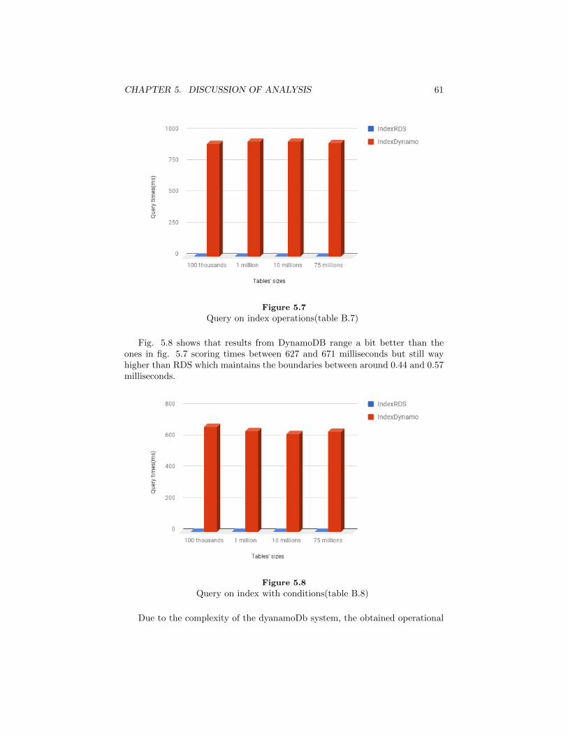
CHAPTER 5. DISCUSSION OF ANALYSIS 61
Figure 5.7
Query on index operations(table B.7)
Fig. 5.8 shows that results from DynamoDB range a bit better than theones in fig. 5.7 scoring times between 627 and 671 milliseconds but still wayhigher than RDS which maintains the boundaries between around 0.44 and 0.57milliseconds.
Figure 5.8
Query on index with conditions(table B.8)
Due to the complexity of the dyanamoDb system, the obtained operational

CHAPTER 5. DISCUSSION OF ANALYSIS 62
times are very much the expected behavior of the DynamoDB system. Dyan-moDb being a noSQL database, owns a lot of moving parts on the backend.What has been mainly experienced throughout the analysis is that at any time,a given request could vary in times due to the network traffic/latency on AmazonDynamoDB backend nodes. Being present numerous components on a network,such as DNS servers, switches, load balancers, and others can generate delaysanywhere in the life of a given request due to which it is not possible to providean exact operational time for DyanmoDb requests.
Dynamodb only promises to customers in average a single digit millisecondlatency on a single item API calls such as getItem, updateItem, DeleteItem andputItem only when the item size is less than 4KB for reads and 1KB for writes.For batches operations such as query and Scan, since the number of resultsreturned by respective API calls varies due to which it is difficult to provide anyprecise latency values.
DynamoDB latency promises are only made for the server side latency i.e. itis monitored from the moment the requests hits the DynamoDB end-point tillit fetches the result, and sends it back to the end-point. Any delays/latenciesoccurred during the time request reaches from client instance to the end-pointor return is not calculated in the DynamoDB latency.
In our case, the latencies obtained might be more than the DynamoDBlatency promises since it involves the client side latency as well, or they mighthave been minor fluctuations from the service side.
5.4 Scalability
Even if DynamoDB does not have any limit on the amount of data being storedin a table, while RDS fixes the limit at 6TB per table, under the scalabilitypoint of view, from all the bar charts exposed so far it could be admitted thatboth databases guarantee high scalability. On one hand, DynamoDB scalesautomatically spreading the data over sufficient machine resources to meet stor-age requirements. On the other hand, RDS allows to set from 1,000 IOPS to30,000 IOPS per DB Instance for scalability reasons. Both databases are ableto maintain roughly the same query time with the increase in size of the tablesperforming the exactly the same operation.

Chapter 6
Conclusions and futurework
6.1 Conclusions
Nowadays, web application can generate and consume huge amounts of data.They might start with just a few users and grow drastically to millions creatingthousands of write/read operations per seconds and generating a large amountof gigabytes(if not terabytes) per day. Due to this, scalability is not an optionanymore, it is a must.
At this time, new RDBMSs providing improved horizontal scaling have beenintroduced in the market, however, the SQL systems still strive to provide hori-zontal scalability without getting rid of SQL itself and ACID transactions. Thisfact represents one of the main reasons why many companies are moving theirdatabase layers to a NoSQL solution. Subsection 2.6.1 presented several typesof available NoSQL solutions describing some of their key features. The rightone to chose strictly depends on company’s use cases. In general talking, if theapplication needs to handle a lot of data, it will be limited when using MySQLor other RDBMS by their structure. The right choice between NoSQL andRDBMS only depends on the actual needs of the application. In fact, some ap-plications might be well served by using both. On one hand, if the applicationrequire to store data that does not lend itself well to a relational schema (treestructures, schema-less JSON representations, and so on) that can be lookedup against a single key or a key/range combination then DynamoDB (or someother NoSQL store) would likely be the best bet. On the other hand, to have awell-defined schema for application’s data that can fit well in a relational struc-ture and the flexibility to query the data in a number of different ways (addingindexes as necessary of course) is strictly required, then RDS might be a bettersolution(answer to RQ1). Our choice in respect of Amazon DynamoDB wasguided by the structure of the dataset in the tables subjects of the analysis.Such dataset could be easily interpreted as a key-value and since the system’s
63
CHAPTER 6. CONCLUSIONS AND FUTURE WORK 64
migration was about to be done in favor of AWS, DynamoDB has been chosenfor the purpose of the benchmarking analysis.
In the overall considerations, DynamoDB results highly available and sta-ble against failures thanks to the automatic replication and failover policies.It shows an excellent scalability and aggregated throughput, although, it guar-antees the maximum throughput instead of latency, users will not get fasterresponse if they use low throughput. This means that with a large amount ofusers it will not work as fast as it would with fewer users, instead, with few usersit will work as slow as with many. This ”feature” has been built to avoid usersfrom reaching easily the provisioned throughput by lowering down the latencyin the case they have only fewer users [50].
RDS is also a Managed service, however the use case for both of them isentirely different. Thus, query speeds in DynamoDB and RDS also dependsupon a lot of different factors as explained in chapter 5. DynamoDB as NoSQLstorage layer is mainly considered for lookup queries (and not Join queries).
Our benchmarking analysis exposed in chapter 5 shows that choosing aNoSQL database to speed up query times is not always the right chose to bedone(at least with our implementation and tables’ structure). In our case, Dy-namoDB have not met our expectation. We expected to see its query times tobe faster in fetching records than writing them into the tables, thus, comparedwith Amazon RDS, most of the queries performed were slower than the lat-ter with the exception of queries related to write operations where DynamoDBunexpectedly jumped up in speed resulting overall faster than RDS. The mainbenefit for using DynamoDB as a NoSQL store is that the user gets guaran-teed read/write throughput at whatever level required without having to worryabout managing a clustered data store. If, for example, the application requiresa thousand reads/writes per second, DynamoDB table can just be provisionedfor that level of throughput and the developer does not really have to worryabout the underlying infrastructure. Moreover, it allows the user to start smalland arrange capacity’s table as long as the requirements increase without beingexposed to downtimes(research question RQ2).
Having said that and looking at the overall picture under another pointof view, taking care of database scalability, management, performance, andreliability does not cover all the lacks from the functionalities that can be foundin a relational database. In DynamoDB querying data is extremely limitedespecially about non-indexed data. Not to have a good support for complextransactions or complex queries like JOINs could be a big concern for a workloadthat requires this range of capabilities even if SQL JOIN operations, for example,kill performance, especially when is required to aggregate data across such joins.Thinking at the situation where there are dozens of joins with thousands ofsimultaneous users, an RDBMS system would start to fall apart. On the otherhand, in NoSQL databases complex data relations have to be managed on thecode/cache layer and sometimes it can be hard to do. Furthermore, on matterof data integrity, while the idea of fluid data may be interesting and desirableto begin with, some applications’ workloads may be better suited if used withan unchangeable structure. Strong type might save the whole database when a
CHAPTER 6. CONCLUSIONS AND FUTURE WORK 65
little bug attempts to destroy it and in DynamoDB, being schema-less, most ofthe time anything that can go wrong, it exactly does(research question RQ3).
Moreover, as explained from Eric Brewer in [42], a system could maintainonly two out of three among consistency, availability and partition-tolerance andin case of NoSQL systems, generally, consistency is the one that gives up. Mostof the time, the lack of consistency brings to better performance and scalabilitybut for some kinds of applications and transactions, like the ones involved onbanking services, it could be a real issue(research question RQ4).
One more concern to take into account is the limit in matter of indexes inDynamoDB. Changing or adding Local Secondary Indexes on-the-fly is impossi-ble without creating a new table. Global Secondary Indexes creation is availableup to five meaning that if more indexes are required workarounds have to beimplemented in the code. Moreover, once the read/write capacity units are set,Amazon allows to decrease them only four times per day while there is no limitsof provisioned IOPS in RDS for MariaDB.
Eventually, NoSQL databases are targeted to a specific set of applicationsscenarios. They will not and cannot replace RDBMSs, they can address certainlimitations and are a complement to deal with issues such as complexity, per-formance, and scalability. Once again, the right database to be used should bechosen according to the data model and dataset to be used with.
6.2 Future work
As this work aimed to analyze the performance testing with just simple queries,there are several possibilities for further extensions and improvements. One ofthe most interesting aspects that could be explored would be the behaviour ofDynamoDB in presence of queries involving multiple tables with JOINs oper-ations. This would require a precise schema to be implemented, for example,involving redundancy of data, to test if effectively a NoSQL database can dealwith lack of JOIN’s operator.
Another interesting topic for future works could be the implementation ofour benchmarking analysis on other NoSQL databases besides DynamoDB, likedocument stores or column stores presented in subsections 2.6.1.2 and 2.6.1.4.This would give the opportunity to compare the performance of them with realworld data.
Other further investigations about performance improvements could be madeby adding caching, that in key-value stores seems to be an excellent use casewhen running a medium to high volume dataset where data is mostly read.
Moreover, the benchmarking analysis involved in this project could also bereplicated in other clouds solutions like OpenNebula [58] or Microsoft Azure [53]as long as they provides services for NoSQL databases with similar features ofthe ones own by Amazon DynamoDB.

Bibliography
[1] Replicated data management in distributed systems. 1992.
[2] Object-relational dbmss: The next great wave. IBM Redbooks, 1996.
[3] Ims premier. IBM Redbooks, 2000.
[4] Database Management Systems 3nd edition. McGraw-Hill Higher Educa-tion, 2003.
[5] Bigtable: A distributed storage system for structured data. ACM Trans-actions on Computer Systems, 26(2), June 2008.
[6] Cassandra: A decentralized structured storage system. Operating SystemsReview, 44(2):35–40, April 2010.
[7] Database System Concepts 6th Edition. McGraw-Hill, January 2010.
[8] Sql and nosql databases. International Journal of Advanced Research inComputer Science and Software Engineering, 2(8):20–27, August 2012.
[9] Type of nosql databases and its comparison with relational databases. In-ternational Journal of Applied Information Systems, 5(4), March 2013.
[10] Benchmarking couchbase for interactive applications with high in-memorydata loads. March 2014.
[11] Relational vs. nosql databases: A survey. International Journal of Com-puter and Information Technology, 03(3):598–601, May 2014.
[12] Database migration from structured database to non-structured database.International Journal of Computer Applications (ICRTAET 2015), 2015.
[13] Nosql databases: a survey and decision guidance. https://medium.
baqend.com/, August 2016.
[14] Sql versus nosql movement with big data analytics. pages 59–66, December2016.
66
BIBLIOGRAPHY 67
[15] Geeta Pattun Abdul Haseeb. A review on nosql: Applications and chal-lenges. International Journal of Advanced Research in Computer Science,8(1), Jan-Feb 2017.
[16] Veronika Abramova, Jorge Bernardino, and Pedro Furtado. Which nosqldatabase? a performance overview. Open Journal of Databases(OJDB),1(2), 2014.
[17] Inc. Amazon Web Services. Amazon aws. https://aws.amazon.com/.
[18] Inc. Amazon Web Services. Amazon ec2. https://aws.amazon.com/ec2/?nc2=h_m1.
[19] Inc. Amazon Web Services. Boto3. https://boto3.readthedocs.io.
[20] Inc. Amazon Web Services. Amazon dynamodb. http://docs.aws.
amazon.com/amazondynamodb/latest/APIReference/Welcome.html,2017.
[21] Inc. Amazon Web Services. Local secondary indexes. http://docs.aws.
amazon.com/amazondynamodb/latest/developerguide/LSI.html, 2017.
[22] Inc. Amazon Web Services. Paginating the results. http:
//docs.aws.amazon.com/amazondynamodb/latest/developerguide/
Query.html#Query.Pagination, 2017.
[23] Inc. Amazon Web Services. Partitions and data distribution. http:
//docs.aws.amazon.com/amazondynamodb/latest/developerguide/
HowItWorks.Partitions.html, 2017.
[24] Charles W. Bachman. The programmer as navigator. Communications ofthe ACM, 16(11):653–658, November 1973.
[25] Alan Beaulieu. Learning SQL, 2nd Edition. O’REILLY, April 2009.
[26] Paul Beynon-Davies. Database Systems 3rd edition. PALGRAVEMACMILLAN, 2004.
[27] Alexandru Boicea, Florin Radulescu, and Laura Ioana Agapin. Mongodbvs oracle – database comparison. pages 330–335, 2012.
[28] E. F. Codd. A relational model of data for large shared data banks. 1970.
[29] E. F. Codd. Further normalization of the data base relational model. Au-gust 1971.
[30] E. F. Codd. Recent investigations into relational data base systems. April1974.
[31] E. F. Codd. The relational model for database management: version 2.Addison-Wesley Longman Publishing Co., Inc., Boston, MA, USA, 1990.

BIBLIOGRAPHY 68
[32] Oracle Corporation. How mysql uses indexes. https://dev.mysql.com/
doc/refman/5.7/en/mysql-indexes.html, 2017.
[33] Tanmay Deshpande. Mastering DynamoDB. PACKT, August 2014.
[34] Ramez Elmasri and Shamkant Navathe. Fundamentals of Database Sys-tems. Addison-Wesley Publishing Company, USA, 6th edition, 2010.
[35] Django Software Foundation. Django 1.9.4. https://www.djangoproject.com.
[36] Django Software Foundation and individual contributors. https://docs.
djangoproject.com/en/1.11/ref/models/instances/, 2005-2017.
[37] Python Software Foundation. socket — low-level networking interface.https://docs.python.org/2/library/socket.html, 1990-2017.
[38] Python Software Foundation. Time access and conversions. https://docs.python.org/2/library/time.html, 2017.
[39] The Apache Software Foundation. Cassandra. http://cassandra.
apache.org/.
[40] The Apache Software Foundation. Couchdb. http://couchdb.apache.
org/.
[41] Shahram Ghandeharizadeh, Jason Yap, and Hieu Nguyen. Strong consis-tency in cache augmented sql systems. pages 181–192, 2014.
[42] Seth Gilbert and Nancy Lynch. Brewer’s conjecture and the feasibilityof consistent, available, partition-tolerant web services. SIGACT News,33(2):51–59, June 2002.
[43] Github. Titan. http://titan.thinkaurelius.com/.
[44] Venkat N. Gudivada, Dhana Rao, and Vijay V. Raghavan. Nosql systemsfor big data management. pages 190–197, 2014.
[45] Amazon Web Services Inc. Amazon dynamodb. https://aws.amazon.
com/documentation/dynamodb/.
[46] Amazon Web Services Inc. Amazon relational database service. http:
//docs.aws.amazon.com/AmazonRDS/latest/UserGuide/Welcome.html.
[47] Maria Indrawan-Santiago. Database research: Are we at a crossroad? re-flection on nosql. pages 45–51, 2012.
[48] Charles Kozierok. The TCP/IP Guide: A Comprehensive, Illustrated In-ternet Protocols Reference. No Starch Press, San Francisco, CA, USA,2005.

BIBLIOGRAPHY 69
[49] Neal Leavitt. Will nosql databases live up to their promise? Computer,43(2):12–14, February 2010.
[50] Tonglin Li, Xiaobing Zhou, Kevin Br, and Ioan Raicu. Distributed key-value store on hpc and cloud systems, 2013.
[51] LinkedIn. Project voldemort. http://www.project-voldemort.com/.
[52] MariaDB. About xtradb. https://mariadb.com/kb/en/mariadb/
about-xtradb/, 2017.
[53] Microsoft. Microsoft azure. https://azure.microsoft.com, 2017.
[54] Inc. MongoDB. Mongodb. https://www.mongodb.com.
[55] Inc. Neo Technology. Neo4j. https://neo4j.com/.
[56] Jaroslav Pokorny. Nosql databases: A step to database scalability in webenvironment. pages 278–283, 2011.
[57] Dan Pritchett. Base: An acid alternative. Queue, 6(3):48–55, May 2008.
[58] OpenNebula Project. Opennebula. https://opennebula.org/, 2017.
[59] M. R. Patra R. P. Padhy and S. C. Satapathy. Rdbms to nosql: Reviewingsome next-generation non-relational database’s. International Journal ofAdvances in Engineering, Science and Technology, 11(1015):15–30, 2011.
[60] REDISLABS. Redis. https://redis.io/.
[61] Stuart Sechrest. An introductory 4.3bsd interprocess communication tuto-rial. Unix Programmer’s Supplementary Documents, 1, April 1986.
[62] Werner Vogels. Eventually consistent. 2008.
[63] Adrienne Watt. Database Design. B.C. Open Textbook project, October2012.

Appendix A
Standard Deviation onmeasurements
Figure A.1
Standard Deviation on Writeoperations
Figure A.2
Standard Deviation on Deleteoperations
Figure A.3
Standard Deviation on Updateoperations
Figure A.4
Standard Deviation on Readoperations
70
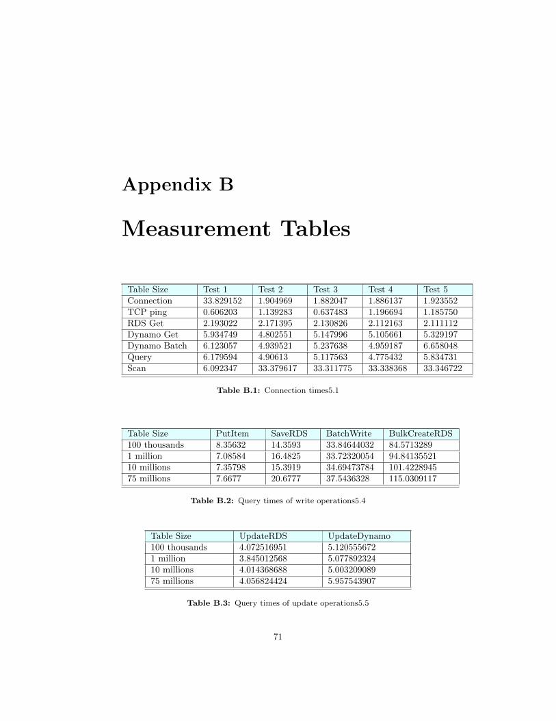
Appendix B
Measurement Tables
Table Size Test 1 Test 2 Test 3 Test 4 Test 5Connection 33.829152 1.904969 1.882047 1.886137 1.923552TCP ping 0.606203 1.139283 0.637483 1.196694 1.185750RDS Get 2.193022 2.171395 2.130826 2.112163 2.111112Dynamo Get 5.934749 4.802551 5.147996 5.105661 5.329197Dynamo Batch 6.123057 4.939521 5.237638 4.959187 6.658048Query 6.179594 4.90613 5.117563 4.775432 5.834731Scan 6.092347 33.379617 33.311775 33.338368 33.346722
Table B.1: Connection times5.1
Table Size PutItem SaveRDS BatchWrite BulkCreateRDS100 thousands 8.35632 14.3593 33.84644032 84.57132891 million 7.08584 16.4825 33.72320054 94.8413552110 millions 7.35798 15.3919 34.69473784 101.422894575 millions 7.6677 20.6777 37.5436328 115.0309117
Table B.2: Query times of write operations5.4
Table Size UpdateRDS UpdateDynamo100 thousands 4.072516951 5.1205556721 million 3.845012568 5.07789232410 millions 4.014368688 5.00320908975 millions 4.056824424 5.957543907
Table B.3: Query times of update operations5.5
71

APPENDIX B. MEASUREMENT TABLES 72
Table Size DeleteItemDynamo DeleteItemRDS BatchDeleteDynamo100 thousands 5.13576 4.346059582 8.4419250491 million 5.5659 4.687962605 4.94503974910 millions 5.7765 5.232647829 5.02896308975 millions 6.37653 4.749733263 5.138158798
Table B.4: Query times of delete operations5.6
Table Size RDS Get GetItem BatchGet Query100 thousands 2.86985 4.47293 5.47253 4.574571 million 2.36627 5.66778 6.23182 4.4711910 millions 2.27676 4.55873 4.44165 4.34975 millions 2.2687 4.50455 4.50312 4.42043
Table B.5: Query times of read operations5.3
Table Size RDS Get GetItem BatchGet Query Scan100 thousands 2.86985 4.47293 5.47253 4.57457 70.26851 million 2.36627 5.66778 6.23182 4.47119 67.917310 millions 2.27676 4.55873 4.44165 4.349 72.512975 millions 2.2687 4.50455 4.50312 4.42043 99.7251
Table B.6: Read operation measurements with Scan5.2
Table Size IndexRDS IndexDynamo100 thousands 0.42135403 900.556842101 million 0.28062441 921.5954400210 millions 0.28042024 921.4193265875 millions 0.29035418 908.36303211
Table B.7: Query times of read operations on index5.7
Table Size IndexRDS IndexDynamo100 thousands 0.57958679 671.151326581 million 0.49703823 644.9146550610 millions 0.45861939 627.1797017475 millions 0.44604116 642.31136806
Table B.8: Query times of read operations on index with conditions5.8