Performance Evaluation of a Mathematical

Programming Based Clustering Algorithm for a

Wireless Ad Hoc Network Operating in a Threat

Environment

by

Esra Cosar

Department of Industrial Engineering

University at Buffalo (SUNY)

Thesis submitted to the faculty of the Graduate School

of the University at Buffalo (SUNY) in partial fulfillment

of the requirements for the degree of

Master of Science

February 2005

i

Abstract

A distributed sensing network consists of more than one spatially separated sen-

sors, each with possibly different characteristics and not all of them sensing the same

environment. The sensors are mobile and change location with time. In this work,

we evaluate the operational level performance of a mathematical programming based

clustering algorithm that is developed for locating a given number of clusterheads in

a wireless ad hoc sensor network such that maximum information can be gathered

from the sensors under hostile conditions. This methodology is also compared with a

representative approach (MOBIC) from the clustering algorithms that have been pro-

posed in the literature. Both small (30 nodes) and medium sized (60 nodes) networks

are used for comparison purposes.

As a result of the numerical studies, it is concluded that the CG heuristic performs

much better in terms of sensor coverage when compared to the original MOBIC

algorithm. During 3 scenarios out of 64, MOBIC provides slightly better coverage,

however the objective function values corresponding to these scenarios indicate that

the CG heuristic outperforms by 46.06%. According to the packet level analysis

performed using OPNET, 94% of the time no packets are lost due to collision during

the simulations for both the CG heuristic and MOBIC. In addition, only a small

percentage of packets sent by the sensors is lost due to the probability of link failure

or the collision of packets transmitted to the same receiver channel of a clusterhead

(1.83% for CG and 2.22% for MOBIC).

ii

Acknowledgment

I would like to express my sincere gratitude to my advisors, Dr. Rajan Batta and

Dr. Rakesh Nagi, for their constant support and guidance. I am thankful to them

for sharing their valuable knowledge and expertise with me.

I would like to thank Mehmet Can, for always being there for me. All my friends

at UB, especially Seda, Pelin, Elif, Abhay, Aykut and Kerem deserve a special thanks

for making my stay in Buffalo enjoyable.

Finally, I wish to thank my parents and my younger sister Didem. I would not

have been where I am now without their love, encouragement, inspiration and uncon-

ditional support.

Esra Cosar

iii

To

My Parents

iv

Contents

List of Figures vii

List of Tables viii

1 Introduction and Literature Review 1

1.1 Introduction . . . . . . . . . . . . . . . . . . . . . . . . . . . . . . . . 1

1.2 Literature Review on Wireless Ad Hoc Networks . . . . . . . . . . . . 4

1.2.1 Network Topology . . . . . . . . . . . . . . . . . . . . . . . . 8

1.2.2 Location Management . . . . . . . . . . . . . . . . . . . . . . 10

1.2.3 Routing Management . . . . . . . . . . . . . . . . . . . . . . . 11

1.3 Literature Review on Clustering Algorithms . . . . . . . . . . . . . . 13

1.4 Objectives of the Research . . . . . . . . . . . . . . . . . . . . . . . . 19

1.5 Outline of the Thesis . . . . . . . . . . . . . . . . . . . . . . . . . . . 21

2 Clustering Algorithms 22

2.1 Capacitated Dynamic MEXCLP Model . . . . . . . . . . . . . . . . . 22

2.1.1 Solution Methodology . . . . . . . . . . . . . . . . . . . . . . 25

2.2 MOBIC Clustering Algorithm . . . . . . . . . . . . . . . . . . . . . . 27

3 Performance Evaluation Studies 31

3.1 Design of Experiments . . . . . . . . . . . . . . . . . . . . . . . . . . 31

3.1.1 Assumptions . . . . . . . . . . . . . . . . . . . . . . . . . . . . 31

v

3.1.2 Input Parameters . . . . . . . . . . . . . . . . . . . . . . . . . 32

3.1.3 Fractional Factorial Design . . . . . . . . . . . . . . . . . . . . 33

3.1.4 Random Problem Instance Generation . . . . . . . . . . . . . 34

3.1.5 Performance Metrics . . . . . . . . . . . . . . . . . . . . . . . 35

3.2 Network Model Simulation . . . . . . . . . . . . . . . . . . . . . . . . 36

3.2.1 Network Simulator . . . . . . . . . . . . . . . . . . . . . . . . 36

3.2.2 OPNET Network Model . . . . . . . . . . . . . . . . . . . . . 38

3.2.3 Packet Level Performance Metrics . . . . . . . . . . . . . . . . 40

4 Experiment Results 43

4.1 Column Generation Heuristic Results . . . . . . . . . . . . . . . . . . 43

4.1.1 Discussion of the Results . . . . . . . . . . . . . . . . . . . . . 51

4.2 MOBIC Results . . . . . . . . . . . . . . . . . . . . . . . . . . . . . . 51

4.2.1 Modified MOBIC Algorithm . . . . . . . . . . . . . . . . . . . 53

4.2.2 Discussion of the Results . . . . . . . . . . . . . . . . . . . . . 54

4.3 Network Simulation Results . . . . . . . . . . . . . . . . . . . . . . . 57

5 Conclusions 71

Appendices 73

A Numerical Results 73

vi

List of Figures

1.1 Some applications of Distributed Sensing and Fusion [33] . . . . . . . 2

1.2 A typical scenario [26] . . . . . . . . . . . . . . . . . . . . . . . . . . 4

1.3 3-tier Hierarchical Network Architecture . . . . . . . . . . . . . . . . 9

1.4 Flat Network Architecture . . . . . . . . . . . . . . . . . . . . . . . . 10

1.5 An example of the periodic clustering algorithm [7] . . . . . . . . . . 18

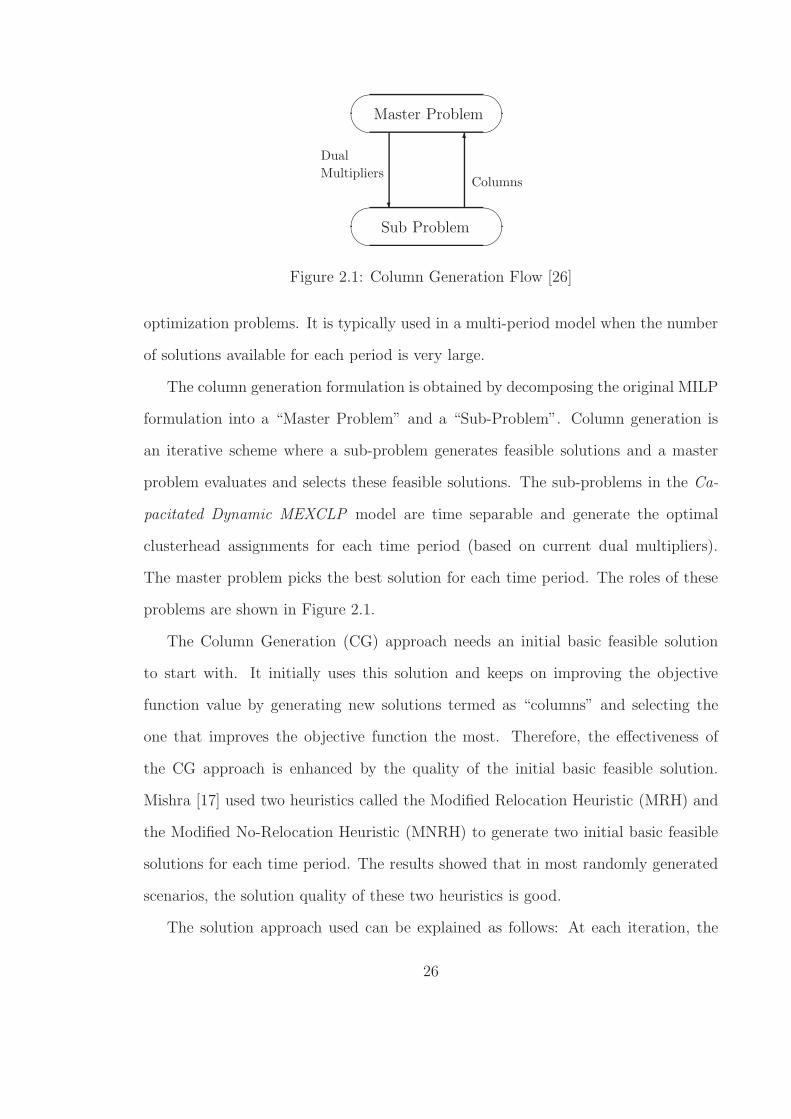
2.1 Column Generation Flow [26] . . . . . . . . . . . . . . . . . . . . . . 26

2.2 Successive Rx Power Measurements [4] . . . . . . . . . . . . . . . . . 28

2.3 A Node with m Neighbors [4] . . . . . . . . . . . . . . . . . . . . . . 29

4.1 CG Main Effect Plot for Total Number of Assignments . . . . . . . . 46

4.2 CG Interaction Plot for Total Number of Assignments . . . . . . . . . 46

4.3 CG Main Effect Plot for Total Number of Single Coverage . . . . . . 47

4.4 CG Interaction Plot for Total Number of Single Coverage . . . . . . . 48

4.5 CG Main Effect Plot for Total Number of Double Coverage . . . . . . 49

4.6 CG Interaction Plot for Total Number of Double Coverage . . . . . . 49

4.7 CG Main Effect Plot for Triple or More Coverage . . . . . . . . . . . 50

4.8 CG Interaction Plot for Triple or More Coverage . . . . . . . . . . . . 50

4.9 Original MOBIC vs. Modified MOBIC . . . . . . . . . . . . . . . . . 55

4.10 Histogram of Differences . . . . . . . . . . . . . . . . . . . . . . . . . 56

4.11 Number of CH Changes: CG vs. MOBIC . . . . . . . . . . . . . . . . 57

vii

List of Tables

3.1 Fractional Factorial Design: Factor Levels . . . . . . . . . . . . . . . 34

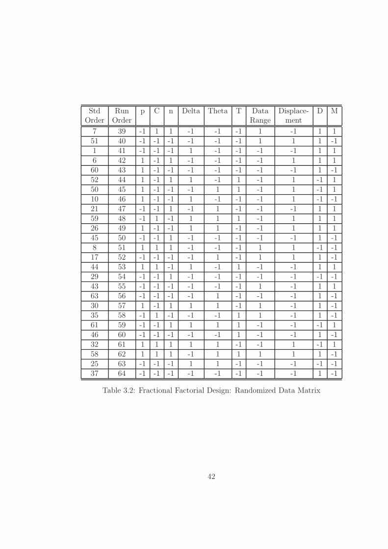
3.2 Fractional Factorial Design: Randomized Data Matrix . . . . . . . . 42

4.1 Coverage Results for the Column Generation Heuristic . . . . . . . . 61

4.2 Percentage of Sensors Covered for the Column Generation Heuristic . 63

4.3 Significant Factors and Interactions: Total Number of Assignments . 63

4.4 Significant Factors and Interactions: Total Number of Single Coverage 64

4.5 Significant Factors and Interactions: Double Coverage . . . . . . . . . 64

4.6 Significant Factors and Interactions: Triple or More Coverage . . . . 64

4.7 Coverage Results for the Original MOBIC Algorithm . . . . . . . . . 66

4.8 Coverage Results for the Modified MOBIC Algorithm . . . . . . . . . 68

4.9 Results for the Packet Level Analysis . . . . . . . . . . . . . . . . . . 70

A.1 Maximum Number of Assignments Possible for Each Scenario . . . . 73

A.2 Objective function values for the CG Results . . . . . . . . . . . . . . 74

A.3 Percentage of Sensors Covered for the MOBIC Algorithm . . . . . . 76

A.4 Objective function values for MOBIC Version1 Results . . . . . . . . 76

A.5 Objective function values for MOBIC Version2 Results . . . . . . . . 77

A.6 Percentage of Sensors Covered for the Modified MOBIC Algorithm . 79

A.7 Objective function values for the modified MOBIC Version1 Results . 79

A.8 Objective function values for the modified MOBIC Version2 Results . 80

viii

Chapter 1

Introduction and Literature

Review

1.1 Introduction

A distributed sensing network consists of more than one spatially separated sensors,

each with possibly different characteristics and not all of them sensing the same envi-

ronment. An example is a military sensor network that detects enemy movements to

track enemy targets (such as planes, missiles etc.) and detects the presence of haz-

ardous material (such as poison gases or radiation, explosions, etc.). Some examples

of distributed sensing are shown in Figure 1.1.

In this work, a critical scenario encountered in a military application is considered.

This scenario is that of a battlefield. The sensors on the area could be soldiers, radars

or tanks on the ground, sonars (on ships) or submarines in the water, unmanned

aircraft vehicles or other airborne surveillance systems in the air. These sensors are

the sources of information that can be used to recognize threats to the system and

thus, help the task of gathering intelligence. The information collected from these

sensors is then assimilated through the process of Data Fusion.

Data Fusion can be formally defined as “a multilevel, multifaceted process dealing

with detection, association, correlation, estimation and combination of data and in-

formation from multiple sources to achieve refined state and identity estimation, and

1

Figure 1.1: Some applications of Distributed Sensing and Fusion [33]

complete and timely assessments of situations and threats” [15].

The combination of data from multiple sensors is called Multisensor Data Fusion

Process. The fusion of data from more than one sensor provides a better judgement

of the scenario since multiple input is obtained to verify the authenticity of the in-

formation. Because of the fact that the sensors can lie at a distance from each other,

the information taken from these sensors has to be sent to the locations where it is

going to be fused.

The process of fusion over a distributed sensing environment might be centralized

or decentralized. In centralized data fusion, the data is fused at a single processor.

This fusion process can be carried out by Command and Control Centers or even

on a smaller scale by satellites, etc. In decentralized data fusion, the data from

groups of sensors (referred to as clusters) are processed together at their corresponding

fusion centers (referred to as clusterheads) and then broadcast or transmitted to other

clusterheads.

2

In the military setting, the clusterheads are generally represented by Airborne

Warning and Control Systems (AWACS). However, they could also be a tank in a

regiment or the captain of an infantry unit.

In a non-wartime situation with all the sensors being static and the fusion loca-

tion (clusterhead) fixed, the data transfer can take place through wired networks.

However, during wartime or for battlefield surveillance, all the sensors and the clus-

terheads may be fixed or mobile. In this case, the network has to rely on wireless

transfer of information. Since there exists no fixed infrastructure or predetermined

connectivity between the sensors and clusterheads, this network should be considered

as a wireless ad hoc network. Ad hoc networks are described in detail in Section 1.2.

In the military scenario we consider, the data transfer takes place through wireless

communication. Since the sensors are mobile, they may move out of the range of the

clusterheads or the bandwidth restrictions might disrupt or disconnect the commu-

nication link between them. In addition, a communication link is prone to enemy

attack. Thus, a link has an associated probability of failure (which might include

instrument malfunction, foliage effects and terrain effects). Therefore, it is extremely

desirable that each sensor should have multiple coverage, i.e. each sensor should be

covered by more than one clusterhead. This ensures maximum network reliability in

case of a breakdown of the communication link between a sensor and its clusterhead.

When such a failure occurs, the sensors should retain the capability to switch to a

backup clusterhead.

Since all sensors are capable of moving and can change their position with time,

relocation of clusterheads (AWACS) is necessary to achieve maximum coverage of

sensor data. A typical scenario including sensors and clusterheads is given in Figure

1.2.

As it was mentioned before, the sensors are in general spatially separated and may

3

Figure 1.2: A typical scenario [26]

not be in close proximity of one another. Hence, an important question is: “Where

should the data fusion take place?” In other words, how should the clusterheads be

placed so as to maximize the information obtained from the sensors? The data from

which sensors should be processed together by the same clusterhead?

A large variety of algorithms have been proposed in the literature to answer the

questions stated above. The objective of this work is to study the performance of a

mathematical programming based clustering algorithm that is developed for locating

a given number of clusterheads in a wireless ad hoc sensor network and compare it

with other clustering algorithms.

In the following section, a comprehensive review of wireless ad hoc networks is

provided and the algorithms that are developed for clustering the sensors in these

networks are presented.

1.2 Literature Review on Wireless Ad Hoc Net-

works

Ad hoc networks are a key in the evolution of wireless networks. They are typically

composed of equal nodes, which communicate over wireless links without any central

4

control [3]. An ad hoc network is formally defined as a self-organizing, multi-hop

wireless network which relies neither on fixed infrastructure nor on predetermined

connectivity. All the entities in an ad hoc network can be mobile. The network

topology may change rapidly and unpredictably over time depending on the node

mobility.

A Mobile Ad Hoc Network (MANET) can be defined as an autonomous collection

of mobile users that communicate over relatively bandwidth constrained wireless links

[34]. The network is decentralized, where all network activity including discovering

the topology and delivering messages must be executed by the nodes themselves, i.e.,

routing functionality will be incorporated into mobile nodes.

The set of applications for MANETs is diverse, ranging from small, static net-

works that are constrained by power sources, to large-scale, mobile, highly dynamic

networks. Regardless of the application, MANETs need efficient distributed algo-

rithms to determine network organization, link scheduling, and routing.

Some examples of wireless ad hoc networks are the following [35]:

1. Military sensor networks to detect and gain as much information as possible

about enemy movements, explosions, and other phenomena of interest.

2. Sensor networks to detect and characterize Chemical, Biological, Radiological,

Nuclear and Explosive (CBRNE) attacks and material.

3. Sensor networks to detect and monitor environmental changes in plains, forests,

oceans, etc.

4. Wireless traffic sensor networks to monitor vehicle traffic on highways or in

congested parts of a city.

5. Wireless surveillance sensor networks for providing security in shopping malls,

parking garages, and other facilities.

5

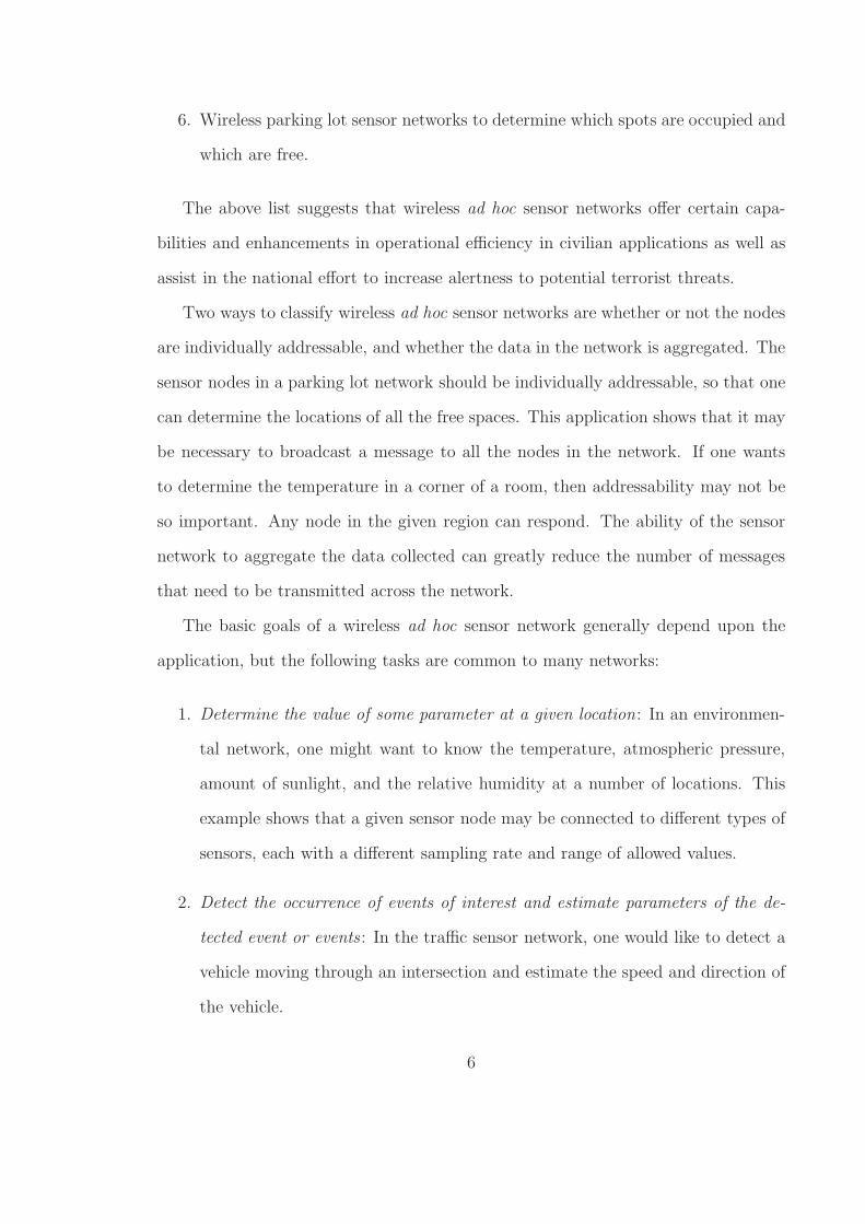
6. Wireless parking lot sensor networks to determine which spots are occupied and

which are free.

The above list suggests that wireless ad hoc sensor networks offer certain capa-

bilities and enhancements in operational efficiency in civilian applications as well as

assist in the national effort to increase alertness to potential terrorist threats.

Two ways to classify wireless ad hoc sensor networks are whether or not the nodes

are individually addressable, and whether the data in the network is aggregated. The

sensor nodes in a parking lot network should be individually addressable, so that one

can determine the locations of all the free spaces. This application shows that it may

be necessary to broadcast a message to all the nodes in the network. If one wants

to determine the temperature in a corner of a room, then addressability may not be

so important. Any node in the given region can respond. The ability of the sensor

network to aggregate the data collected can greatly reduce the number of messages

that need to be transmitted across the network.

The basic goals of a wireless ad hoc sensor network generally depend upon the

application, but the following tasks are common to many networks:

1. Determine the value of some parameter at a given location: In an environmen-

tal network, one might want to know the temperature, atmospheric pressure,

amount of sunlight, and the relative humidity at a number of locations. This

example shows that a given sensor node may be connected to different types of

sensors, each with a different sampling rate and range of allowed values.

2. Detect the occurrence of events of interest and estimate parameters of the de-

tected event or events: In the traffic sensor network, one would like to detect a

vehicle moving through an intersection and estimate the speed and direction of

the vehicle.

6

3. Classify a detected object : Is a vehicle in a traffic sensor network a car, a mini-

van, a light truck, a bus, etc.

4. Track an object : In a military sensor network, track an enemy tank as it moves

through the network.

In these four tasks, an important requirement of the sensor network is that the

required data be disseminated to the proper end users. In some cases, there are fairly

strict time requirements on this communication. For example, the detection of an

intruder in a surveillance network should be immediately communicated to the police

so that necessary action can be taken.

Wireless ad hoc sensor network requirements include the following [19]:

• Scalability : The networks might consist of as many as 100, 000 nodes and so,

scalability is a major issue.

• Sensor mobility/self-organization: The sensors can be in motion, the sensor

location at any instant of time being known deterministically, probabilistically

or might even be unknown. Given the large number of nodes and their potential

placement in hostile locations, it is essential that the network be able to self-

organize; manual configuration is not feasible.

• Connectivity : In general, the initial establishment of connection between a pair

of sensors does not guarantee communication between them at all instances

during the time horizon under consideration. This is because there might be

link failures caused by instrument malfunctions, lack of energy, terrain effects

or jamming.

• Low energy use: Since in many applications the sensor nodes will be placed in a

remote area, service of a node may not be possible. In this case, the lifetime of a

7

node may be determined by the battery life, thereby requiring the minimization

of energy expenditure.

• Collaborative signal processing : To improve the detection/estimation perfor-

mance, it is often quite useful to fuse data from multiple sensors. This data

fusion requires the transmission of data and control messages, and so it may

put constraints on the network architecture.

• Querying ability : A user may want to query an individual node or a group

of nodes for information collected in the region. Depending on the amount of

data fusion performed, it may not be feasible to transmit a large amount of

the data across the network. Instead, various local clusterheads will collect the

data from a given area and create summary messages. A query will be directed

to the clusterhead nearest to the desired location.

Sanchez et al. [31] discuss some of the issues involved in ad hoc networks and

broadly classify them as follows:

1. Network Topology

2. Location Management

3. Routing Management

1.2.1 Network Topology

Typically, the topology in an ad hoc network is either flat or hierarchical.

Hierarchical Architecture

In a hierarchical topology, nodes are partitioned into groups called clusters. Within

each cluster, a node is chosen to perform the function of a clusterhead. Depending

on the number of hierarchies, such networks can have one or more tiers or levels.

8

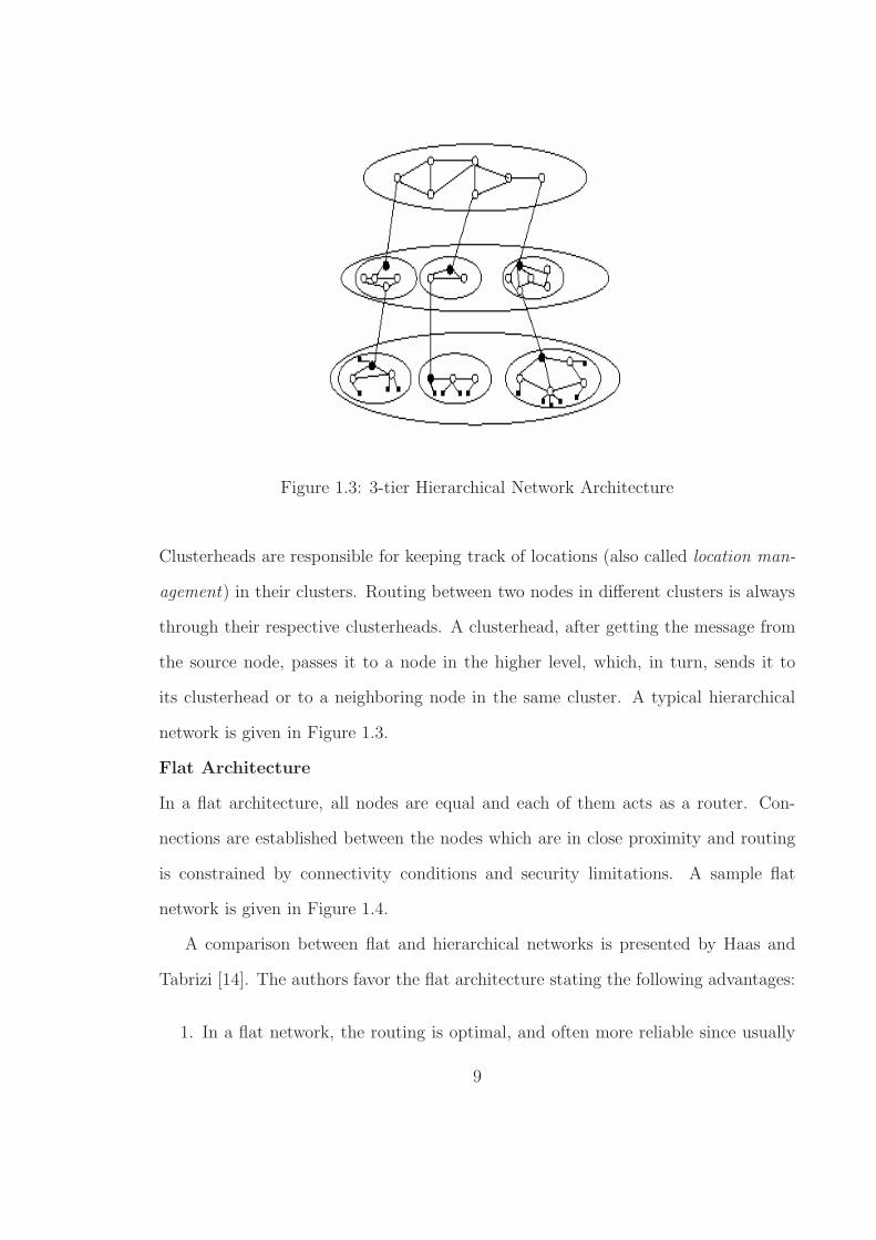
Figure 1.3: 3-tier Hierarchical Network Architecture

Clusterheads are responsible for keeping track of locations (also called location man-

agement) in their clusters. Routing between two nodes in different clusters is always

through their respective clusterheads. A clusterhead, after getting the message from

the source node, passes it to a node in the higher level, which, in turn, sends it to

its clusterhead or to a neighboring node in the same cluster. A typical hierarchical

network is given in Figure 1.3.

Flat Architecture

In a flat architecture, all nodes are equal and each of them acts as a router. Con-

nections are established between the nodes which are in close proximity and routing

is constrained by connectivity conditions and security limitations. A sample flat

network is given in Figure 1.4.

A comparison between flat and hierarchical networks is presented by Haas and

Tabrizi [14]. The authors favor the flat architecture stating the following advantages:

1. In a flat network, the routing is optimal, and often more reliable since usually

9

Figure 1.4: Flat Network Architecture

more than one path exist between source and destination nodes. However, in

hierarchical networks, clusterheads are single points of failure and therefore,

these routes are more susceptible to attack.

2. Nodes in a flat network transmit at a significantly lower power than the trans-

mission power of clusterheads in hierarchical networks. This results in more

network capacity, less expense in power and larger degree of Low Probability of

Interception/Low Probability of Detection.

3. In a flat network, no overhead is associated with dynamic addressing, cluster

creation and maintenance and mobile location management.

On the other hand, a major disadvantage of flat networks is that they are not scal-

able. Mobility management is simpler in a hierarchical network since the clusterheads

keep the databases containing locations of all nodes in their clusters.

1.2.2 Location Management

Location management deals with keeping track of locations of all the mobile nodes in

the network. In order to keep current locations of the nodes, it is necessary to maintain

a large database with periodic or continuous updating. Location Management can be

classified on the basis of this update into static and dynamic strategies. In static

10

strategies, the locations are updated at a predetermined set of locations; whereas in

dynamic strategies, the nodes (end-users) determine when an update should be gen-

erated based on its movement. Kasera and Ramanathan [18] consider the location

management problem in a hierarchically organized multi-hop wireless network where

all nodes are mobile. Clusterheads work as location managers for their clusters to

maintain the association database and perform other functions. Their location man-

agement mainly deals with location updating, location finding and switch mobility.

Location updates occur when one of the following events happen [18, 30]:

1. End-user reaffiliates to some other switch.

2. The switch to which the end-user is affiliated moves to some other cluster.

3. Cluster reformation such as cluster splitting or merging.

Location management does not seem to work in a flat network since there is

nothing equivalent to clusterheads. However, Haas and Tabrizi [14] have made a case

for flat networks with zone routing as described in the next section.

1.2.3 Routing Management

In ad hoc networks, routing has to be determined dynamically. The literature for

routing protocols is divided into three parts:

• Proactive or Table Driven Routing Protocol,

• Reactive or On-Demand Routing Protocol, and

• Hybrid Protocol.

In a proactive protocol, the route between each pair of nodes is continuously main-

tained in a tabular format. This table is updated on a continuous basis, recording the

11

changes in the network topology. Thus, the delay in determining the route is minimal,

but maintaining the table is costly and wasteful for both time and bandwidth. Some

of the protocols cited in the literature are as follows:

1. Destination-Sequenced Distance-Vector Routing (DSDV) [28],

2. Wireless Routing Protocol (WRP) [21], and

3. Clusterhead Gateway Switch Routing (CGSR) [8].

In a reactive protocol, routes are determined on a need to basis. When a packet is

to be delivered from source node to the destination node, a route discovery procedure

is initiated and a route is determined through a global search procedure. This results

in large delays and may therefore be unacceptable in applications where long routing

delays cannot be allowed. Some of the protocols cited in the literature are as follows:

1. Ad Hoc On-Demand Distance Vector Routing (AODV) [29],

2. Associativity Based Routing (ABR) [39],

3. Dynamic Source Routing (DSR) [16], and

4. Temporally Ordered Routing Algorithm (TORA) [24].

Hybrid protocols combine the advantages of both proactive and reactive proto-

cols. Haas [13] proposed Zone Routing Protocol (ZRP), a hybrid protocol based on

the notion of routing zone. In this protocol, each node proactively determines the

routes between itself and nodes within its routing zone. Thus, whenever a demand

arises, the route can be determined among the node not in the routing zone. ZRP

requires only a small number of query messages, as these messages are routed only to

peripheral nodes, omitting all other nodes within the routing zones. As the zone ra-

dius is significantly smaller than the network radius, the cost of updating the routing

12

information for the zone topologies is small compared to a global proactive mecha-

nism. In addition, ZRP is much faster than a global reactive discovery mechanism,

as the number of nodes queried is very small compared to the global flooding process.

Finally, the path determined by ZRP needs less number of hops and therefore is more

stable.

1.3 Literature Review on Clustering Algorithms

Clustering is an important technique for imposing hierarchy and organization in a

mobile ad hoc network. It helps to reduce the complexity in managing the information

about the mobile nodes. Clustering of nodes in ad hoc networks are done in order

to use the wireless resources efficiently by reducing the congestion in the network,

and also for the purpose of proper location and routing management. A large variety

of algorithms have been proposed in the literature for clustering in ad hoc networks.

Some common features of these clustering algorithms can be stated as follows [26]:

• Stability : There should not be frequent changes in clusterhead assignments due

to the mobility of the nodes. The clusterheads should be comparatively less

mobile.

• Load Balancing : The clusters should neither be densely populated nor scarcely

populated.

• Battery Power : Clusterheads consume more power than the other nodes. There-

fore, the assignments should not cause excessive drainage of some nodes over

others.

• Transmission Range and Signal Strength: A clusterhead should have sufficient

transmission range and signal power to reach all the nodes in its cluster.

13

The selection of clusterheads optimally is an NP-hard problem [2]. Therefore,

most of the existing solutions are based on heuristic approaches. These approaches

can be broadly classified as being graph based and geographical based. In graph based

heuristics, the network is viewed as a graph; whereas geographical based heuristics use

Global Positioning System (GPS) to accurately determine the location and velocity

of the nodes in the network. In general, the message cost of maintaining clusters (at

all speeds) is slightly smaller for graph based clustering, whereas the percentage of

nodes uncovered (unmanaged) by clusterheads is smaller for geographical clustering

[7]. If we have a situation where the nodes have widely varying transmission ranges,

graph based clustering is better since geographical clustering does not consider this

information.

Graph Based Clustering

There are several graph based clustering algorithms proposed in the literature. These

can be briefly explained as follows:

• Highest Degree Heuristic: “Degree” of a node is defined as the number of

nodes within its transmission range. The degree based heuristic is a modified

version of the work in Parekh [23]. In this approach, the node with highest

degree (highest connectivity) is selected as clusterhead and with all the nodes

within its transmission range forms the cluster. The selection process continues

until all nodes are assigned to some clusterhead. Here, load balancing is poor,

but the stability of the clusters is good.

• Lowest ID Heuristic: Each node is assigned a distinct ID. Periodically, the

nodes broadcast the list of the nodes that they can hear (i.e. the nodes that fall

into their transmission range, including themselves). In this heuristic, a node

which only hears nodes with ID higher than itself assumes the responsibility of

a clusterhead and with all the nodes within its transmission range forms the

14

cluster [11]. The lowest-ID node that a node hears is its clusterhead, unless

the lowest-ID specifically gives up its role as a clusterhead (deferring to a yet

lower ID node). The selection process continues until all nodes have a desig-

nated clusterhead. According to Chiang [8], lowest ID heuristic provides a more

stable cluster formation than the highest degree heuristic, but causes excessive

drainage of lower ID nodes.

• Node Weight Heuristic: In this heuristic, a weight of -υ is assigned to a

node with a speed of υ units [1]. The clusterhead selection criteria is the same

as the highest degree heuristic. It is shown that a stable solution is obtained

using this heuristic, i.e. the number of clusterhead reassignments is smaller

when compared to the highest degree and lowest ID heuristics.

• Weight Based Clustering Algorithm: A weight based clustering algorithm

is proposed by Chatterjee et al. [6] where the weight of each node is updated

periodically. Here, a weight is assigned to each of the features such as Load

Balancing, Battery Power, Signal Strength and Mobility. The solution obtained

from this algorithm has less reassignment of clusterheads when compared to the

previously mentioned heuristics. This algorithm also provides the flexibility of

adjusting the weighing factors according to the system needs.

• MOBIC Clustering Algorithm: Basu et al. [4] proposed this distributed

algorithm for mobile ad hoc networks (MANETs). This algorithm is based on

a relative mobility metric for clusterhead selection. All nodes send a “Hello”

message to all of their neighbors and calculate their relative mobility metric by

a formula using the signal strength of the received message. Each node shares

its mobility metric with other nodes in its transmission range and the node with

least relative mobility assumes the position of a clusterhead. The results in the

15

paper show that when compared to the Lowest ID heuristic, there is a reduction

of as much as 33% in the rate of clusterhead changes owing to the use of the

proposed technique.

All the above approaches assume reliable communication among the nodes in the

network.

Geographical Based Clustering

The algorithm proposed by Chen et al. [7] takes advantage of the GPS (Global Posi-

tioning Systems ) and uses this system to find the latitude, longitude and (relative)

velocity of the nodes. Here, the nodes are split into clusters based on their spatial

density. Each cluster is a rectangular box, and one of the more centrally located nodes

within that box is selected as the clusterhead. Node mobility tends to change the

spatial density of the nodes and therefore, over time, the clusters need to be reformed.

The clustering algorithm works in two stages. The first stage, Central Periodic

Clustering Algorithm is a periodic procedure to form clusters for the entire network

using spatial density as a guide. This stage is carried out by a central global manager.

This stage is divided into three main steps:

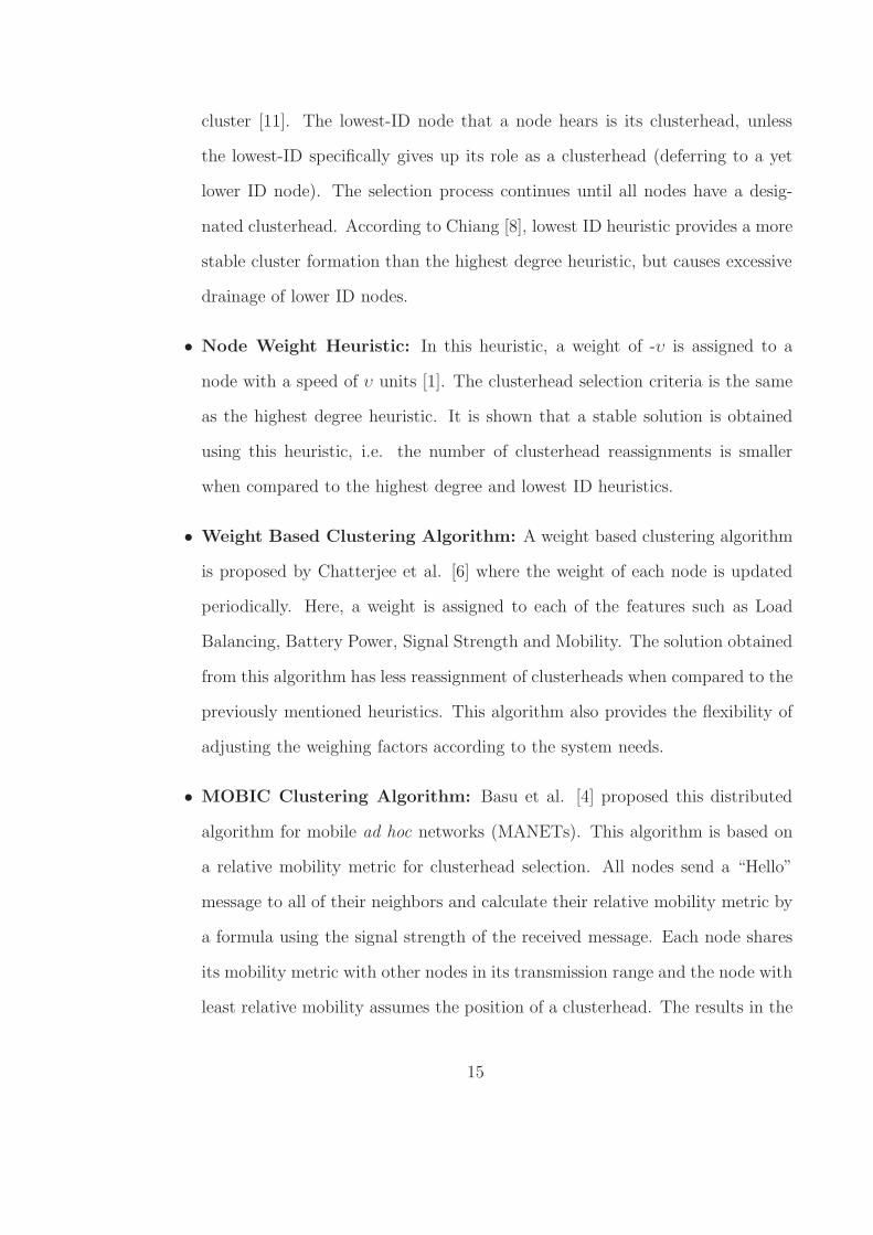
1. Box Generation: The ad hoc network box is divided into vertical and horizontal

strips. The number of nodes that lie in each strip is counted and a bar graph is

constructed for the horizontal and vertical dimension. Next, the sparse areas in

the bar graph are examined and the region is split into small boxes along these

sparse areas. As a result, nodes in areas where the node density is high fall in

the same cluster.

2. Box Size Refinement: This step checks the size of box and restricts the ratio of

length to breadth of the boxes to 1.5. The rationale for this rule is to prevent

the formation of long and skinny boxes.

16

3. Node Density Adjustment: Removes boxes with no nodes in it and merges boxes

with less nodes and splits boxes with high node density.

After clustering is complete, the global manager selects a clusterhead for each clus-

ter based on locality (e.g., as close to the center as possible) or some other metric (e.g.,

maximum available battery power). It then multicasts the clustering information to

these clusterheads.

In Figure 1.5, a small ad hoc network consisting of 20 nodes is considered and the

clusters are formed using the Periodic Clustering Algorithm.

The second stage, Cluster Maintenance is a maintenance algorithm executed

locally within each cluster between two executions of the periodic protocol. The

outcomes of this stage include changes in cluster membership (add new members or

remove departed members), changes in clusterhead responsibility (when a clusterhead

moves away), merging two clusters into one (if the spatial density in each is small)

and splitting dense clusters into smaller ones.

In the paper [7], it is demonstrated that when the geographical based clustering

algorithm is used, the percentage of nodes uncovered by clusterheads remains well

below 10% for all speeds and network sizes. This algorithm also assumes reliable

communication among the nodes.

We know that the fusion process demands a highly reliable and stable network

architecture for collecting and processing data from all the mobile sensors. However,

there is always a possibility that the links between the nodes may fail. As it was men-

tioned before, none of the clustering heuristics incorporate this possibility of failure,

they all assume that the links between nodes are reliable and data can be communi-

cated between them at all times. However, Patel et al. [25] proposed a mathematical

programming approach for dynamic clustering of the sensors considering the unreli-

ability of the links. This approach aimed to design a flexible network architecture

17

Figure 1.5: An example of the periodic clustering algorithm [7]

that can reorganize itself to capture the dynamics of sensor movement for efficient

data fusion. The problem modeled in this work is referred as the Dynamic Maximum

Expected Covering Location Problem (MEXCLP).

Dynamic MEXCLP Model

The mathematical programming approach proposed by Patel et al. [25] is based on a

variation of a maximal expected covering location model due to Daskin [10]. In this

work, a Mixed Integer Linear Programming (MILP) model is constructed for finding

the optimal location strategies for the clusterheads over the entire time horizon. It

is assumed that sensor movement patterns are known. A trade-off between the need

to provide maximal expected sensor coverage in a hostile environment and the cost

of frequent relocation of clusterheads is explicitly sought. Unreliability of the links is

also considered. After the model construction, a solution method that can perform

well in terms of both solution quality and time is developed.

18

This model assumes that data fusion and bandwidth requirements can always

be met by the clusterheads. However, in reality, some sensors generate enormous

amounts of data (e.g., imagery data) that consume significant fusion capacity. On

the other hand, other intelligent sensors (e.g., tracking radar) generate relatively

much less data and transmit tracks opposed to detailed scan data. Mishra [19] made

modifications to the basic model proposed by Patel [25] to incorporate the capac-

ity restrictions for the clusterheads and called this model the Capacitated Dynamic

MEXCLP Model. A modified column generation (CG) heuristic is developed to solve

this problem. It was noted that addition of the capacity constraints significantly in-

creased the complexity of the problem, however computational results indicated that

CG performs faster than standard commercial solvers and the typical optimality gap

for large size problems is less than 10%. The complete mathematical formulation of

this problem and the solution procedure are given in detail in Section 2.1.

1.4 Objectives of the Research

In this work, we deal with a communication network problem of finding suitable

solutions of clusterheads (e.g. AWACS) for collecting data from multiple mobile

sensors spread over a geographically dispersed area for the purpose of data fusion.

The Capacitated Dynamic MEXCLP model proposed by Mishra [19] incorporates all

the issues of interest, such as the possibility of link failure, mobility of the system

entities, etc. A Column Generation heuristic is adopted as a solution methodology

and numerical studies showed that it solves the problem with a reasonable accuracy,

efficiently. Other clustering algorithms proposed in the literature are divided into two

main classes: Graph based and geographical based.

The objectives of this work can be summarized as follows:

1. To study the performance of the Column Generation heuristic developed for the

19

Capacitated DMEXCLP model at the detailed operational level.

2. To compare this methodology with a representative approach from graph based

and geographical based schemes.

For the comparison purpose, one of the clustering algorithms proposed in the liter-

ature is chosen. In Section 1.3, it is mentioned that both the weight based clustering

algorithm and MOBIC result in a more stable network configuration when compared

to the other graph based heuristics. We know that this stability of the clusters is a key

issue considered in the Capacitated Dynamic MEXCLP model. When we compare

these two graph based approaches taking into consideration this objective, we see

that MOBIC gives the emphasis to the issue of minimal reassignment (relocation) of

clusterheads since it chooses the nodes with lowest relative mobility as clusterheads,

whereas weight based approach gives weight to measures other than stability (i.e.

load balancing). Therefore, MOBIC seems to be a better choice for the comparison

with the Column Generation heuristic developed for Capacitated MEXCLP model.

When MOBIC is compared to the geographical based algorithm, it is seen that

the geographical based algorithm does not focus on forming stable clusters and may

result in frequent clusterhead relocations. However, MOBIC tries not to relocate

clusterheads by selecting a node that is less mobile relative to its neighbors for the

role of a clusterhead. Therefore, the geographical based algorithm is eliminated from

further comparison studies since it does not have a comparable objective with Ca-

pacitated Dynamic MEXCLP model. As a result, MOBIC algorithm is chosen as the

representative of the clustering algorithms and the numerical studies are carried out

for the Column Generation heuristic and the MOBIC clustering algorithm.

The performance of these chosen algorithms is evaluated in two aspects. Since

“coverage” is one of the most important measures of Quality of Service (QoS) of a

sensor network, the other key objective of our work is to provide maximum coverage

20

of sensors by the clusterheads chosen. Therefore, we first compare these algorithms

evaluating how they perform in terms of the coverage of the sensors in the network.

Secondly, we test the reliability of the networks constructed. Therefore, we develop

a simulation model with one of the commercially available network simulators and

integrate the solution methodology of the clustering algorithms that are chosen and

validate the packet-level performance of the clusters formed by these algorithms under

realistic (simulated) conditions.

The software chosen for network simulations is OPNET Modeler 9.0. It is a

very powerful modeling and simulation platform, allowing users to design and study

communication networks, devices, protocols and applications with flexibility and scal-

ability [37]. Since this network simulator provides a close-to-real-world network en-

vironment, it is widely being used in defense applications. A separate module of

the modeler called “Wireless Module” is used in this work to create mobile ad hoc

networks.

1.5 Outline of the Thesis

Chapter 2 presents the details of the clustering algorithms that are chosen for per-

formance evaluation studies. The experiments designed and the network simulation

model constructed using OPNET are discussed in Chapter 3. In Chapter 4, soft-

ware implementation for selected solution methodologies is discussed and detailed

results for the experimental studies are presented. Finally, conclusions drawn from

the analysis are discussed in Chapter 5.

21

Chapter 2

Clustering Algorithms

In this section, we provide detailed information about the Capacitated Dynamic

MEXCLP model developed by [19] and the Column Generation algorithm used to

solve this problem. In addition to this, we present the other clustering algorithm

chosen for the performance evaluation, MOBIC [4].

2.1 Capacitated Dynamic MEXCLP Model

Patel et al. [25] modeled the problem under consideration as a covering problem

which maximizes the expected demand covered with a given number of clusterheads

(referred as Dynamic MEXCLP model). The sensors considered here are capable

of moving and change location in time in order to perform the tasks assigned to

them. Since the sensors are mobile, relocation of clusterheads is necessary to achieve

maximum coverage of sensor data. However, to ensure a stable location strategy over

the entire “time horizon”, excessive number of relocations for the entire time horizon

is restricted by associating a cost with every relocation of clusterheads (termed as

relocation cost). In this work, a trade-off between data coverage and relocation cost

is considered. The time horizon is split up into discrete time periods of equal length.

Relocation of clusterheads is permitted only at the beginning of these time periods.

Other than considering all the entities as mobile, another distinctive characteristic

22

of this problem is that the links between the sensors and the clusterheads are prone to

failure. In other words, the possibility of threat in the network is also incorporated into

the model. A threat in the sensor network can affect both a sensor and a clusterhead.

If the threat occurs at a sensor, we only lose communication or receiver obtains false

information from that particular sensor, however, if it happens on a clusterhead,

several sensors will be involved. In the model, it is assumed that each link fails with

equal probability and independently of all other links. This is equivalent to assuming

a constant threat level in the region, i.e. no specific knowledge of enemy positions.

What this means is that when a sensor needs to use a communication link to send

measurement data or tracks to its clusterhead, it is not able to do so with a constant

and known probability p (threat level). To ensure successful communication in such

a threat environment, multiple coverage is necessary for some important sensors.

Patel [25] developed the model as a communications network, however one im-

portant aspect was not considered: Bandwidth. Building on the Dynamic MEXCLP

model, Mishra [19] developed the Capacitated Dynamic MEXCLP model by incorpo-

rating capacity constraints for the clusterheads.

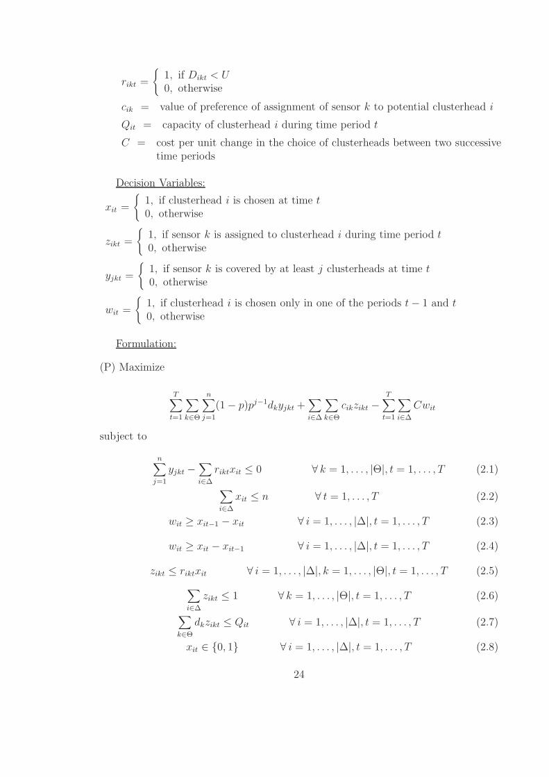
The new model with the capacity restrictions is as follows [19]:

Parameters:

∆ = set of potential clusterheads

Θ = set of sensors

n = maximum number of clusterheads to be located (chosen)

T = number of time periods in the horizon under consideration

U = the distance beyond which a sensor is considered “uncovered”

Dikt = distance between potential clusterhead i and demand node (sensor) kat time t

dk = demand per period of node k

p = probability of a link failure per period (between any clusterhead and sensor)

(0 < p < 1)

23

rikt =

{

1, if Dikt < U0, otherwise

cik = value of preference of assignment of sensor k to potential clusterhead i

Qit = capacity of clusterhead i during time period t

C = cost per unit change in the choice of clusterheads between two successivetime periods

Decision Variables:

xit =

{

1, if clusterhead i is chosen at time t0, otherwise

zikt =

{

1, if sensor k is assigned to clusterhead i during time period t0, otherwise

yjkt =

{

1, if sensor k is covered by at least j clusterheads at time t0, otherwise

wit =

{

1, if clusterhead i is chosen only in one of the periods t − 1 and t0, otherwise

Formulation:

(P) Maximize

T∑

t=1

∑

k∈Θ

n∑

j=1

(1 − p)pj−1dkyjkt +∑

i∈∆

∑

k∈Θ

cikzikt −T

∑

t=1

∑

i∈∆

Cwit

subject to

n∑

j=1

yjkt −∑

i∈∆

riktxit ≤ 0 ∀ k = 1, . . . , |Θ|, t = 1, . . . , T (2.1)

∑

i∈∆

xit ≤ n ∀ t = 1, . . . , T (2.2)

wit ≥ xit−1 − xit ∀ i = 1, . . . , |∆|, t = 1, . . . , T (2.3)

wit ≥ xit − xit−1 ∀ i = 1, . . . , |∆|, t = 1, . . . , T (2.4)

zikt ≤ riktxit ∀ i = 1, . . . , |∆|, k = 1, . . . , |Θ|, t = 1, . . . , T (2.5)

∑

i∈∆

zikt ≤ 1 ∀ k = 1, . . . , |Θ|, t = 1, . . . , T (2.6)

∑

k∈Θ

dkzikt ≤ Qit ∀ i = 1, . . . , |∆|, t = 1, . . . , T (2.7)

xit ∈ {0, 1} ∀ i = 1, . . . , |∆|, t = 1, . . . , T (2.8)

24

wit ≥ 0 ∀ i = 1, . . . , |∆|, t = 1, . . . , T (2.9)

yjkt ≤ 1 ∀j = 1, . . . , n, k = 1, . . . , |Θ|, t = 1, . . . , T (2.10)

zikt ∈ {0, 1} ∀ i = 1, . . . , |∆|, k = 1, . . . , |Θ|, t = 1, . . . , T (2.11)

Here, the objective function maximizes demand covered and preferential assign-

ment while allowing for relocation of clusterheads over the time horizon. If node k

is covered by m clusterheads at time t, Constraint (2.1) assigns each of the variables

y1kt, y2kt, . . . , ymkt a value of 1 since the objective function is a maximization function

containing the term yjkt. Constraint (2.2) restricts the maximum number of cluster-

heads that can be chosen to n for any time t. Constraints (2.3) and (2.4) determine

the value of wit by assigning 1 to this variable when the choice of clusterhead i changes

between consecutive time periods t− 1 and t. Constraint (2.5) ensures that sensor k

is assigned to clusterhead i only if clusterhead i is chosen and sensor k can be covered

by this clusterhead i. Constraint (2.6) ensures that a sensor is assigned to only one

clusterhead during a time period. Constraint (2.7) is the capacity constraint for each

potential clusterhead for each time period. Constraints (2.8), (2.9),(2.10) and (2.11)

are value and sign restrictions on the variables.

2.1.1 Solution Methodology

The Dynamic MEXCLP is a special case of the Capacitated Dynamic MEXCLP

(corresponding to infinite capacity). Since the Dynamic MEXCLP is NP-hard ([26]),

the Capacitated Dynamic MEXCLP is also NP-hard. Thus, in general, the Capaci-

tated Dynamic MEXCLP is expected to be computationally intensive and tough to

solve. So, there is a need to develop special solution procedures since large problems

(representative of the real world applications) cannot even be read by most solvers.

The Capacitated Dynamic MEXCLP model is solved using the Column Gener-

ation heuristic [17]. This heuristic is a widely used technique to solve large-scale

25

��

��

��

��

?

6

Master Problem

Sub Problem

Dual

MultipliersColumns

Figure 2.1: Column Generation Flow [26]

optimization problems. It is typically used in a multi-period model when the number

of solutions available for each period is very large.

The column generation formulation is obtained by decomposing the original MILP

formulation into a “Master Problem” and a “Sub-Problem”. Column generation is

an iterative scheme where a sub-problem generates feasible solutions and a master

problem evaluates and selects these feasible solutions. The sub-problems in the Ca-

pacitated Dynamic MEXCLP model are time separable and generate the optimal

clusterhead assignments for each time period (based on current dual multipliers).

The master problem picks the best solution for each time period. The roles of these

problems are shown in Figure 2.1.

The Column Generation (CG) approach needs an initial basic feasible solution

to start with. It initially uses this solution and keeps on improving the objective

function value by generating new solutions termed as “columns” and selecting the

one that improves the objective function the most. Therefore, the effectiveness of

the CG approach is enhanced by the quality of the initial basic feasible solution.

Mishra [17] used two heuristics called the Modified Relocation Heuristic (MRH) and

the Modified No-Relocation Heuristic (MNRH) to generate two initial basic feasible

solutions for each time period. The results showed that in most randomly generated

scenarios, the solution quality of these two heuristics is good.

The solution approach used can be explained as follows: At each iteration, the

26

RMP (which is the relaxed master problem with no binary constraints on the vari-

ables) is solved and then, all sub-problems are solved for all time periods. The solu-

tions with favorable reduced cost are simultaneously added to the master problem.

Iterations are terminated if none of the sub-problems provide a solution of favorable

reduced cost. In cases where the CG continues to iterate with a small increase in the

objective function of the RMP, other termination criteria can also be utilized. These

criteria for CG may be terminating when a threshold number of iterations has been

reached or when the gap between RMP and the LP relaxation of (P) is within 2%.

The computational results showed that the addition of bandwidth capacity con-

straints for the clusterheads increases the complexity of the problem by a great extent.

For example, for a problem instance with 150 potential locations (all other parame-

ters remaining same), CPLEX solves the uncapacitated problem quickly, however it

is hard for CPLEX to solve the capacitated case. In addition, % gap between the LP

Relaxation of (P) and the optimal solution is much wider for the capacitated problem.

However, CG method still performs faster than a standard commercial solver and the

typical optimality gap for large problems is less than 10%.

2.2 MOBIC Clustering Algorithm

Basu et al. [4] proposed a distributed clustering algorithm, MOBIC, based on the

use of a new mobility metric which is used as a basis for cluster formation. The basic

idea in this paper is that the clustering process should be aware of the mobility of the

individual nodes with respect to its neighboring nodes. A node should not be elected

a clusterhead if it is highly mobile relative to its neighbors, since, in that situation,

the probability that a cluster will break and that reclustering will happen is high.

In this work, in order to model mobility, they purport that the power level (re-

ceived signal strength) detected at the receiving node, RxPr, is indicative of the

27

} }

}

Y X (new location)

X (old location)�����������

old RxPr

new RxPr

Figure 2.2: Successive Rx Power Measurements [4]

distance between the transmitting and receiving node pairs. Using the ratio of RxPr

between two successive packet transmissions (periodic “hello” messages) from a neigh-

boring node, they obtain knowledge about the relative mobility between the two

nodes. This situation is depicted in Figure 2.2.

The relative mobility metric, M relY (X), at a node Y with respect to X is defined

as:

MrelY (X) = 10 log10

RxPrnew

X→Y

RxProld

X→Y

.

The aggregate local mobility value MY at any node Y is found by calculating the

variance (with respect to zero) of the entire set of relative mobility values M relY (Xi),

where Xi is a neighbor of Y .

MY = var 0(MrelY (X1),M

relY (X2),..., M rel

Y (Xm)) = E[(M relY )2].

Here, a low value of MY indicates that Y is relatively less mobile with respect to

its neighboring nodes. On the contrary, a high value of MY means that Y is highly

mobile with respect to its neighboring nodes. In this algorithm, the nodes that have

a low variance in relative mobilities are candidates for becoming clusterheads.

This distributed, lowest mobility clustering algorithm, MOBIC, can be described

in the following steps:

• All nodes send and receive “Hello” messages to/from their neighbors. Each node

measures the received power levels of two successive “Hello” message transmis-

28

}

}

}

}}

} 6

�

��

���

@@

@@@R

������* Y

X4

Xm

X1X2

X3

MY = f (relative mobility)

Figure 2.3: A Node with m Neighbors [4]

sions from every neighbor and calculates the pairwise relative mobility metric

values. Before sending the next broadcast packet to its neighbors, a node com-

putes the aggregate relative mobility value MY .

• Every node broadcasts its own mobility metric to its 1-hop neighbors and these

MY values are then stored in the neighbor table of each neighbor along with a

timeout period set. When a node receives the aggregate mobility values from

all its neighboring nodes, it compares its own mobility value with those of its

neighbors.

• If a node has the lowest value of M amongst all its neighbors, it assumes the

status of a clusterhead; otherwise it declares itself to be a cluster member.

In case where the mobility metric of two clusterhead nodes is the same, the

clusterhead selection is based on the “Lowest-ID Algorithm” [8] wherein the

node with the lowest ID obtains the status of the clusterhead.

• If two clusterheads move into each other’s range, reclustering is deferred for

Cluster Contention Interval (CCI) to allow for incidental contacts between pass-

29

ing nodes. If the nodes are in transmission range of each other even after the

CCI timer has expired, reclustering is triggered, and the node with the lower

mobility metric becomes the new clusterhead.

In this paper, it is demonstrated that this distributed clustering algorithm leads

to more stable cluster formation than the “least clusterhead change” version of the

well known Lowest-ID clustering algorithm [8]. Using ns-2 simulations, they showed

that there is reduction of as much as 33% in the rate of clusterhead changes owing to

the use of the proposed technique.

30

Chapter 3

Performance Evaluation Studies

In this part of the report, we provide information about the experiments designed

and the network simulation models constructed using OPNET.

3.1 Design of Experiments

For the purpose of evaluating the performance of Column Generation heuristic and

MOBIC, a certain number of simulation experiments are designed, different scenarios

are generated and implemented.

3.1.1 Assumptions

The assumptions related to the scenarios generated are:

1. Sensors and clusterheads are mobile with known velocity vectors.

2. Clusterheads are perfectly reliable while all links have a (identical) steady-state

probability of link failure.

3. Clusterheads are identical in all aspects.

4. Time horizon is divided into equal time periods.

5. Relocation of clusterheads takes place at the beginning of each time period.

31

3.1.2 Input Parameters

The factors governing the problem structure are (refer to [26] and [19]):

• Number of clusterheads that can be chosen at any time period.

• Displacement range: Maximum displacement possible in x, y, z directions per

unit time.

• Displacement: Displacement of the nodes in x, y, z directions per unit time. It

is uniformly generated between 0 and displacement range.

• Clusterhead location range: Defines the region within which the clusterheads

are located at time t = 0. The location of a particular clusterhead at subsequent

time periods is calculated based on the displacement of that clusterhead per unit

time.

• Sensor location range: Defines the region within which the sensors are located

at time t = 0. The location of a particular sensor at subsequent time periods is

calculated based on the displacement of that sensor per unit time.

• Demand data range: This is the interval on which the demand of the sensors

lies.

• Number of potential clusterheads.

• Number of sensors.

• Coverage radius within which a clusterhead can cover a sensor.

• Preference assignment constant: Shows the preference values of the clusterheads

by the sensors.

• Clusterhead capacity: The capacity of the potential clusterheads.

32

• Probability of link failure between the clusterheads and sensors.

• Relocation cost incurred per unit change in the choice of clusterheads between

two successive time periods.

• Length of the time horizon under consideration.

Among the factors explained above, some of them are considered to be constants

during the experimental studies. The clusterhead location range and the sensor lo-

cation range are taken as the interval [0, 500]. The preference assignment constant is

chosen to be 5. Since this factor is a constant, it is assumed that all potential clus-

terheads are equally preferred by the sensors. The remaining factors are considered

to be changing in different scenarios created.

3.1.3 Fractional Factorial Design

In this section, we design experiments to determine how the clustering algorithms

perform under varying factors. The primary motive of this effort is to compare the

algorithms with the responses (explained in Section 3.1.5) at different combinations

of the problem parameters (also referred as factors).

Considering the enormity of the number of the factors, a screening experiment is

performed to determine the insignificant factors and their insignificant higher level

interactions, so that these factors could be taken out and the responses could be

analyzed and explained in terms of the significant factors.

If a full factorial design was to be conducted, 210 experiments would be required.

Instead of this, a 2k−m fractional factorial design of resolution IV is designed as the

screening experiment with a single replicate. Here, k refers to the number of factors

which is 10 and m = 4. The factors that are not considered as constants in the

experimental studies are classified into two categories: Low Level and High Level. By

33

choosing such a design, we assume that the high order interactions are negligible and

this greatly simplifies the problem structure.

The α-level or level of significance considered is 0.05. The values of the factors

chosen for each category are given in Table 3.1.

Factor LevelsFactors Low level (-1) High level (1)

Probability of link failure (p) 0.2 0.7Relocation cost (C) 10 100Number of CHs that can be chosen (n) 5 10Number of potential CHs (Delta) 10 20Number of sensors (Theta) 20 40Length of the time horizon (T) 5 10Demand data range for sensors (Data Range) 10 50Displacement range for the nodes (Displacement) 10 40Coverage radius (D) 150 200CH capacity (M) 40 80

Table 3.1: Fractional Factorial Design: Factor Levels

Design of Fractional Factorial Experiment: MINITAB Results

The screening experiment is carried out using MINITAB and the results are as follows:

Factors: 10 Base Design: 10, 64 Resolution: IV

Runs: 64 Replicates: 1 Fraction: 1/16

Blocks: 1 Center pts (total): 0

Design Generators: G = BCDF, H = ACDF, J = ABDE, K = ABCE

The randomized data matrix generated by MINITAB is given in Table 3.2.

3.1.4 Random Problem Instance Generation

After the combinations of the factor values are determined for 64 runs, the problem

instances (namely, scenarios) are created using Random Problem Instance Generator

module coded in C. This module takes the predetermined values for the preference

assignment constant, clusterhead location range and sensor location range as inputs

34

for all scenarios to be generated. In addition to these, it uses the specified level values

of the factors Delta, Theta, T, Data Range and Displacement to randomly generate

the trajectories of both the clusterheads and the sensors, and the demands of the

sensors. Therefore, the generated scenarios are the networks constituted by a certain

number of sensors and clusterheads, operated over a predetermined time horizon. Due

to the fact that these nodes are both mobile, the scenarios also have the trajectory

information about all the nodes. Finally, the sensors have specific demand values.

The numerical studies for the clustering algorithms chosen are performed using

the problem instances created with this module. The results obtained are discussed

in Chapter 4.

3.1.5 Performance Metrics

After the scenarios are created randomly, the two clustering algorithms (Capacitated

Dynamic MEXCLP and MOBIC) are run and the values of several outputs are col-

lected. We have two sets of performance measures, one related to the coverage of the

sensors by the clusterheads chosen and the other related to the packet-level perfor-

mance of the networks constructed. The measures for the algorithms regarding the

coverage aspect are:

• Total number of sensors covered by the clusterheads (total number of assign-

ments) during the whole time horizon, T : Here, we count the number of sensors

that are assigned to any clusterhead. For instance, if a sensor is assigned dur-

ing 4 periods out of 5, this means that this sensor is counted 4 times in this

calculation.

• Total number of sensors that are covered once (by only one clusterhead): Here,

we count the sensors which are assigned to a clusterhead at a specific time

period and also, which fall into the communication range of only this specific

35

clusterhead that they are assigned to. Again, we sum the numbers over all time

periods.

• Total number of sensors that are covered twice: These are the sensors that are

assigned and among the clusterheads chosen, they can be covered by two of

them.

• Total number of sensors that are covered by at least three clusterheads: The

difference between the total number of sensors assigned and the number of

sensors that can be covered by one or two clusterheads gives the desired number.

The second set of measures that are related to the packet-level performance of the

clustering algorithms are explained in Section 3.2.3.

3.2 Network Model Simulation

After the analysis regarding the coverage issues, packet-level analysis is performed.

A packet level network simulator called OPNET is used for comparative performance

evaluation [37]. The sensor network models with properties specified by the scenarios

generated are constructed using the OPNET Modeler and the performance of the

clusters formed by the clustering algorithms is evaluated under realistic (simulated)

conditions. The following section gives information about the simulation software

chosen, OPNET.

3.2.1 Network Simulator

OPNET Modeler was originally developed at MIT and introduced in 1987 as the

first commercial network simulator. It is based on a series of hierarchical editors that

directly parallel the structure of real networks, equipment and protocols. It is designed

to simulate any required behavior with C/C++ logic in finite state machine (FSM)

36

states and transitions. Being a scalable and efficient simulation engine, it enables very

fast simulation runtimes using advanced acceleration techniques for wired and wireless

models. For example, one can simulate thousands of wireless nodes in a terrain-rich

environment, with dynamic application and routing behavior, at faster-than-realtime

speed on standard workstations [37].

The Wireless module of OPNET extends the functionality of the software with

high-fidelity modeling, simulation and analysis of wireless networks [38]. It integrates

OPNET’s full protocol stack modeling capability with the ability to model all aspects

of wireless transmissions, including:

• Transmitter/receiver characteristics;

• RF propagation (path loss with terrain diffraction, fading, and atmospheric and

foliage attenuation);

• Interference; and

• Interconnection with wire-line transport networks.

This module also includes the capability to model motion in mobile networks,

including ground, airborne, and satellite systems. Mobile node models incorporate

three dimensional position attributes that can change as the simulation progresses.

To sum up, the Wireless module is used to:

• Predict end-to-end performance by modeling and simulating network topology,

traffic, protocols, and end-user applications;

• Evaluate network and QoS configurations before launching new services;

• Design and optimize proprietary wireless protocols such as access control and

scheduling algorithms; and

• Plan mobile network deployments that accurately incorporate terrain effects.

37

3.2.2 OPNET Network Model

After the generation of a scenario, the corresponding network model is constructed

in OPNET. Unlike the Capacitated Dynamic MEXCLP model, MOBIC clustering

algorithm does not consider the threat factor while choosing the clusters and it as-

sumes that the links between sensors and clusterheads are reliable and data can be

communicated between them at all times. In order to make a fair comparison among

these approaches, the unreliability of the links is incorporated into the system during

network simulation stage in OPNET.

The general OPNET model consists of a certain number of sensors and clus-

terheads at specific locations. The nodes can move around in a rectangular region

according to the trajectories determined by the Random Problem Instance Generator

module for that specific scenario. The node movements are discretized for ease of

modeling in a discrete event framework.

There exists wireless communication between the nodes. Each node is modeled

by a “node model” constructed using OPNET Modeler tools. More specifically, the

node model is composed of a process model and a transmitter/receiver. The sensor

nodes and the clusterheads have a transmitter and a receiver, respectively, and they

all have a fixed radio range. Radio channel level details are also modeled and the

properties of the transmitters and receivers (such as transmission rates/frequencies,

bandwidth, power levels, etc.) are specified using the data taken from real-life sensor

types. The specifications of these entities are that of a Tactical Common Data Link

(TCDL) Airborne Data Terminal and are as follows [36]:

• Receiver/transmitter channel:

– Data rate: 10.71 Mbps

– Bandwidth: 430 MHz

38

– Minimum frequency: 14.40 GHz

• Transmitter channel:

– Power: 2 W

The “process model” is essential for a node model. It includes the C codes which

define the states that this specific node can go through and the transitions that

it should follow when predetermined interrupts occur. Therefore, all nodes behave

according to the actions specified in their process models. At the beginning of each

network simulation run, all nodes read the trajectory file generated for that specific

scenario and change their positions accordingly. In addition to this, the sensors read

the file which includes the information about their assignments to the clusterheads

chosen for that specific time period. These assignments are the essential output

obtained when the clustering algorithms are run.

With predetermined intervals (determined by the scan rate of the sensor), an

interrupt is created by OPNET for each sensor. They forward data packets (periodic

sensor transmission strategy) including the target information to the clusterheads

they are assigned to, through the wireless links. In the simulation model, a packet

can be unicast (received only by a specific clusterhead). Whenever a packet is sent

to a clusterhead, another interrupt is automatically created by OPNET for that

specific clusterhead and it examines the package that is sent by one of its sensors (the

package is either accepted or rejected). Data packet processing times are fixed for the

clusterheads since they are assumed to be identical.

As it is mentioned before, the threat factor is also incorporated into the network

models by assigning probabilities for the failure of the links between the sensors and

the clusterheads. p values for the sensors are generated randomly between 0.0 and

1.0. Each sensors has a different p value for each time period, these values are used

39

to determine whether the link between that specific sensors and its clusterhead fails

(is jammed) or not. In the battlefield environment simulated, threat is considered as

being distributed to the region. p values of the sensors are compared with different

base values (the average of these values is the desired p level chosen, either 0.2 as the

low level or 0.7 as the high level) and if they are less than the base value, the link is

assumed to be jammed. With all these specifications, the simulation models are run

for T time steps.

3.2.3 Packet Level Performance Metrics

After the general network model is constructed in OPNET, the scenarios correspond-

ing to 64 experiments are simulated. At the end of these simulation runs, the following

performance measures are collected:

• Total number of packets sent by the sensors to their clusterheads

• Total number of packets received by the chosen clusterheads

• Number/percentage of packet loss due to the failure of the links between the

nodes or the collision of the packets sent to the same receiver channel of a

clusterhead (network traffic flow/congestion)

40

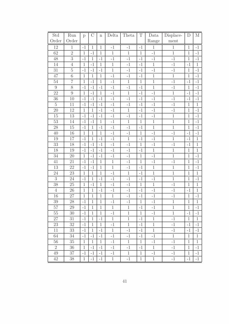
Std Run p C n Delta Theta T Data Displace- D MOrder Order Range ment

12 1 -1 1 1 -1 -1 -1 1 1 1 -162 2 1 -1 1 1 1 1 -1 1 1 -148 3 -1 1 -1 -1 -1 -1 -1 -1 1 -114 4 1 -1 1 1 -1 -1 1 -1 -1 131 5 -1 -1 -1 1 -1 -1 -1 -1 1 -147 6 1 1 1 -1 -1 -1 1 1 1 -154 7 1 -1 1 -1 1 1 1 -1 -1 -19 8 -1 -1 -1 -1 -1 -1 1 -1 1 -122 9 1 -1 1 -1 1 -1 -1 1 -1 -136 10 -1 -1 -1 -1 -1 -1 -1 -1 -1 -15 11 -1 -1 -1 -1 -1 -1 -1 -1 1 120 12 1 1 -1 -1 1 -1 -1 -1 1 -115 13 -1 -1 -1 -1 -1 -1 -1 1 1 -153 14 -1 -1 1 -1 1 1 1 1 1 -128 15 -1 1 -1 -1 -1 -1 1 1 1 -140 16 1 1 1 -1 -1 1 -1 -1 -1 -119 17 -1 1 -1 -1 1 -1 -1 1 -1 133 18 -1 -1 -1 -1 -1 1 -1 -1 -1 118 19 -1 -1 -1 -1 -1 -1 1 1 1 134 20 1 -1 -1 -1 -1 1 -1 1 1 -141 21 -1 -1 1 1 -1 1 -1 -1 1 -113 22 -1 -1 1 1 -1 -1 1 1 1 -124 23 1 1 1 -1 1 -1 1 1 1 13 24 -1 1 -1 -1 -1 -1 -1 1 1 -138 25 1 -1 1 -1 -1 1 1 -1 1 14 26 1 1 -1 -1 -1 -1 -1 -1 -1 116 27 1 1 1 1 -1 -1 -1 -1 1 -139 28 -1 1 1 -1 -1 1 -1 1 1 157 29 -1 1 1 1 1 -1 -1 1 1 -155 30 -1 1 1 -1 1 1 -1 1 -1 -127 31 -1 1 -1 1 1 -1 1 -1 1 123 32 -1 1 1 -1 1 -1 1 -1 -1 -111 33 -1 1 -1 1 -1 -1 1 -1 -1 -164 34 -1 -1 -1 -1 -1 -1 -1 1 1 156 35 1 1 1 -1 1 1 -1 -1 1 12 36 1 -1 -1 -1 -1 -1 1 -1 1 -149 37 -1 -1 -1 -1 1 1 -1 -1 1 -142 38 1 -1 -1 1 -1 1 1 -1 -1 -1

41

Std Run p C n Delta Theta T Data Displace- D MOrder Order Range ment

7 39 -1 1 1 -1 -1 -1 1 -1 1 151 40 -1 -1 -1 -1 -1 -1 1 1 1 -11 41 -1 -1 -1 1 -1 -1 -1 -1 1 16 42 1 -1 1 -1 -1 -1 -1 1 1 160 43 1 -1 -1 -1 -1 -1 -1 -1 1 -152 44 1 -1 1 1 -1 1 -1 1 -1 150 45 1 -1 -1 -1 1 1 -1 1 -1 110 46 1 -1 -1 1 -1 -1 -1 1 -1 -121 47 -1 -1 1 -1 1 -1 -1 -1 1 159 48 -1 1 -1 1 1 1 -1 1 1 126 49 1 -1 -1 1 1 -1 -1 1 1 145 50 -1 -1 1 -1 -1 -1 -1 -1 1 -18 51 1 1 1 -1 -1 -1 1 1 -1 -117 52 -1 -1 -1 -1 1 -1 1 1 1 -144 53 1 1 -1 1 -1 1 -1 -1 1 129 54 -1 -1 1 -1 -1 -1 -1 -1 -1 -143 55 -1 -1 -1 -1 -1 -1 1 -1 1 163 56 -1 -1 -1 -1 1 -1 -1 -1 1 -130 57 1 -1 1 1 1 -1 1 -1 1 -135 58 -1 1 -1 -1 -1 1 1 -1 1 -161 59 -1 -1 1 1 1 1 -1 -1 -1 146 60 -1 -1 -1 -1 -1 1 -1 -1 1 -132 61 1 1 1 1 1 -1 -1 1 -1 158 62 1 1 1 -1 1 1 1 1 1 -125 63 -1 -1 -1 1 1 -1 -1 -1 -1 -137 64 -1 -1 -1 -1 -1 -1 -1 -1 1 -1

Table 3.2: Fractional Factorial Design: Randomized Data Matrix

42

Chapter 4

Experiment Results

After the scenarios are generated and the general simulation model is constructed in

OPNET, the Column Generation heuristic and MOBIC are tested using each scenario.

In this section, the detailed results for these numerical studies are presented.

4.1 Column Generation Heuristic Results

The Column Generation (CG) heuristic is coded in C programming language by Patel

[26]. The commercial software CPLEX (Version 9.0) is used for solving the Relaxed

Master Problem (at each CG iteration) and the Integer Master Problem at the end.

It is also used to solve the LP Relaxation of the Capacitated Dynamic MEXCLP

model. In this work, the experiments are carried out on a Intel Pentium 4 processor

(3200 MHz) with 1 GB RAM operating on Red Hat Linux 9.0 platform.

First of all, the Capacitated Dynamic MEXCLP models corresponding to 64 sce-

narios generated are solved using the CG heuristic. The results obtained regarding

the coverage of sensors are presented in Table 4.1.

Secondly, these numerical values are expressed in percentages in Table 4.2. The

first column of this table presents the percentage of sensor coverage for each scenario.

These percentage values are calculated by dividing the total number of sensors covered

(actual coverage which is displayed in Table 4.1) by the maximum coverage possible

43

for that specific scenario. Maximum coverage is obtained by solving the Maximum

Coverage Location Problem (MCLP) using CPLEX corresponding to each scenario.

The general MCLP is formulated as follows:

Parameters:

n = number of clusterheads that can be chosen during a time period

∆ = set of potential clusterheads

Θ = set of sensors

T = number of time periods in the horizon under consideration

rijt =

{

1, if sensor j is reachable from clusterhead i in time period t0, otherwise

Decision Variables:

xit =

{

1, if clusterhead i is chosen at time t0, otherwise

zjt =

{

1, if sensor j is assigned to a clusterhead during time period t0, otherwise

Formulation:

(P) Maximize

T∑

t=1

Θ∑

j=1

zjt

subject to

∑

i∈∆

xit = n ∀ t = 1, . . . , T (4.1)

zjt −∑

i∈∆

rijtxit ≤ 0 ∀ j = 1, . . . , |Θ|, t = 1, . . . , T (4.2)

xit ∈ {0, 1} ∀ i = 1, . . . , |∆|, t = 1, . . . , T (4.3)

zjt ∈ {0, 1} ∀j = 1, . . . , |Θ|, t = 1, . . . , T (4.4)

Here, the objective function maximizes the number of sensors covered during the

whole time horizon. Constraint (4.1) forces the total number of clusterheads that

can be chosen to be equal to n for any time period t. Constraint (4.2) ensures that

44

if clusterhead i is chosen and sensor j is reachable from this clusterhead, sensor j is

covered by at least one clusterhead and the corresponding zjt variable takes a value

of 1 since the objective function is a maximization function containing the term zjt.

Constraints (4.3) and (4.4) are sign restrictions on the variables.

The optimal values ofT

∑

t=0

Θ∑

j=1

zjt that are obtained when the MCLPs for all 64

scenarios are solved in CPLEX are given in Table A.1 of Appendix A. These values

are the maximum number of assignments possible for each scenario when the capacity

constraint on the clusterheads is not considered.

The second, third and fourth columns of Table 4.2 present the percentage of

sensors covered only once, two times and at least three times, respectively. These

percentages are calculated by dividing the corresponding column values in Table 4.1

by the total number of assignments made for each scenario.

Finally, the objective function values of the Capacitated Dynamic MEXCLP mod-

els corresponding to the generated scenarios are given in Table A.2 of Appendix A.

After the experiments regarding the coverage of sensors are completed, an analysis

of variance (ANOVA) study is performed using MINITAB to see which factors are

significant. Both the individual effect of each factor and the simultaneous impact of

all the factors are evaluated. In addition to this, two-way interaction effects between

the factors are investigated. The ANOVA results obtained are as follows:

Response variable 1: Total number of assignments

In Table 4.3, the factors and the interactions which are found to be significant at

α = 0.05 significance level are listed. It is observed that Theta (number of sensors),

T (length of the time horizon), Data Range (sensor demand values) and D (coverage

radius) directly affect the total number of assignments. The interaction between the

factors Delta (number of potential clusterheads) and Displacement also has an effect

on the response variable.

45

Figure 4.1: CG Main Effect Plot for Total Number of Assignments

Figure 4.2: CG Interaction Plot for Total Number of Assignments

46

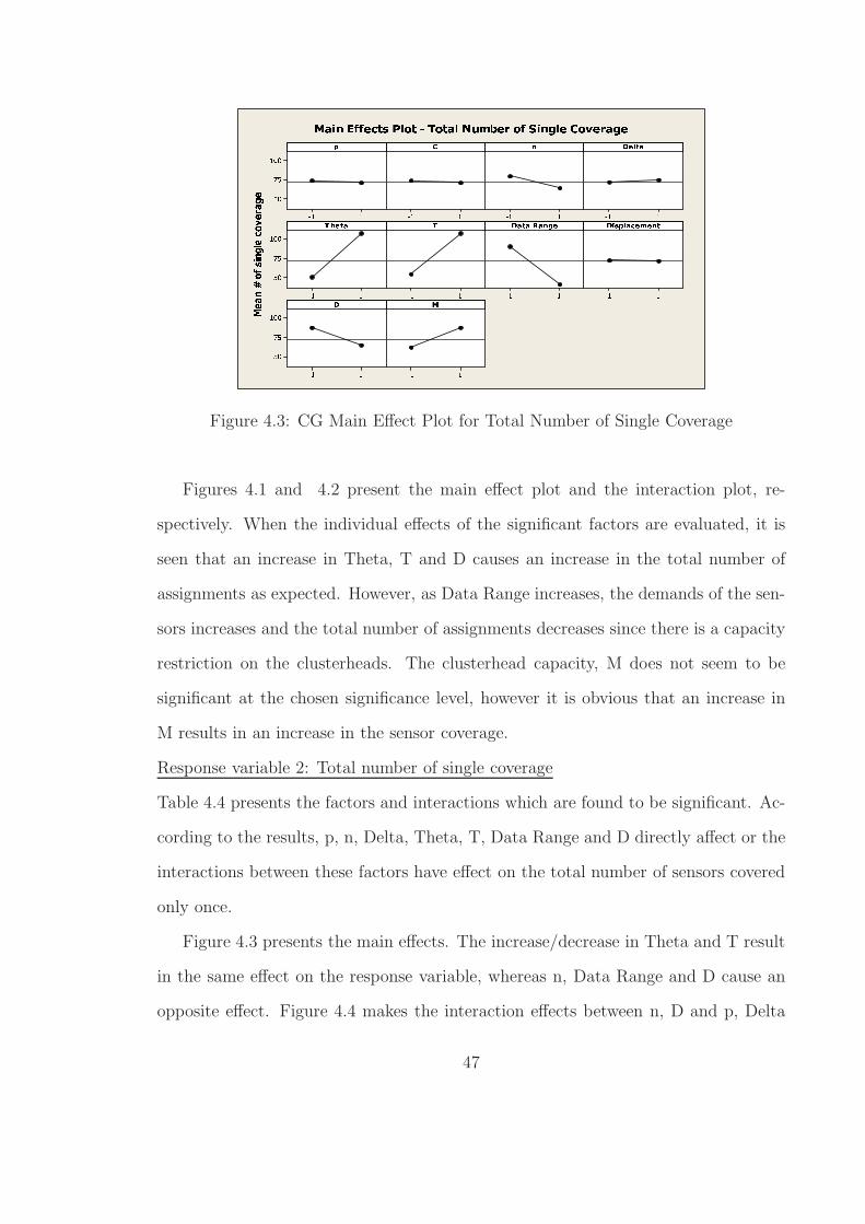
Figure 4.3: CG Main Effect Plot for Total Number of Single Coverage

Figures 4.1 and 4.2 present the main effect plot and the interaction plot, re-

spectively. When the individual effects of the significant factors are evaluated, it is

seen that an increase in Theta, T and D causes an increase in the total number of

assignments as expected. However, as Data Range increases, the demands of the sen-

sors increases and the total number of assignments decreases since there is a capacity

restriction on the clusterheads. The clusterhead capacity, M does not seem to be

significant at the chosen significance level, however it is obvious that an increase in

M results in an increase in the sensor coverage.

Response variable 2: Total number of single coverage

Table 4.4 presents the factors and interactions which are found to be significant. Ac-

cording to the results, p, n, Delta, Theta, T, Data Range and D directly affect or the

interactions between these factors have effect on the total number of sensors covered

only once.

Figure 4.3 presents the main effects. The increase/decrease in Theta and T result

in the same effect on the response variable, whereas n, Data Range and D cause an

opposite effect. Figure 4.4 makes the interaction effects between n, D and p, Delta

47

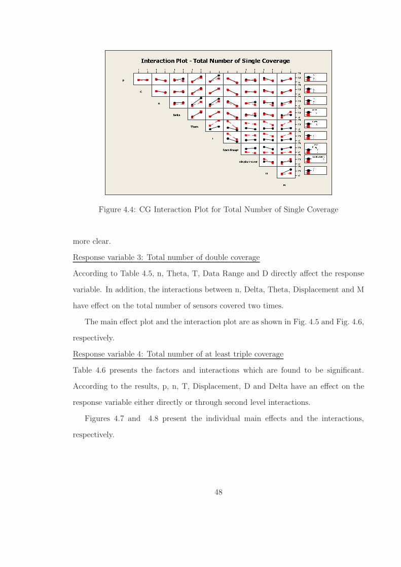
Figure 4.4: CG Interaction Plot for Total Number of Single Coverage

more clear.

Response variable 3: Total number of double coverage

According to Table 4.5, n, Theta, T, Data Range and D directly affect the response

variable. In addition, the interactions between n, Delta, Theta, Displacement and M

have effect on the total number of sensors covered two times.

The main effect plot and the interaction plot are as shown in Fig. 4.5 and Fig. 4.6,

respectively.

Response variable 4: Total number of at least triple coverage

Table 4.6 presents the factors and interactions which are found to be significant.

According to the results, p, n, T, Displacement, D and Delta have an effect on the

response variable either directly or through second level interactions.

Figures 4.7 and 4.8 present the individual main effects and the interactions,

respectively.

48

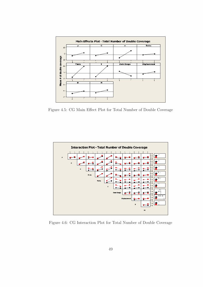
Figure 4.5: CG Main Effect Plot for Total Number of Double Coverage

Figure 4.6: CG Interaction Plot for Total Number of Double Coverage

49

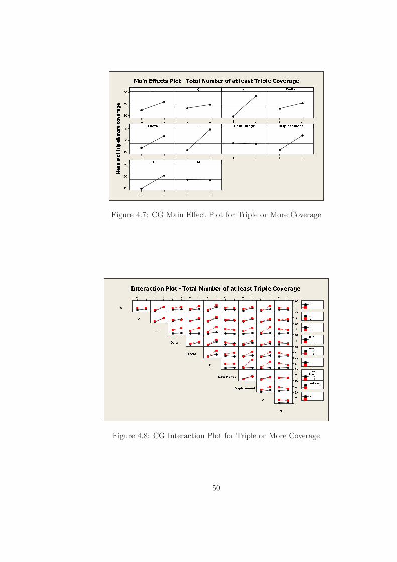
Figure 4.7: CG Main Effect Plot for Triple or More Coverage

Figure 4.8: CG Interaction Plot for Triple or More Coverage

50

4.1.1 Discussion of the Results

The analysis of variance revealed the effect of each factor on the responses chosen.

When these ANOVA tables are examined, it is observed that almost the same factors

affected the responses. Most of the time, the factor M (clusterhead capacity) does

not seem to be a significant factor at the chosen significance level, however, we know

that it is one of the most important factors in determining the sensor assignments.

By comparing Runs 43&64 and 8&36, it is possible to see the effect of the prob-

ability of link failure (p). When p (threat) increases, single coverage decreases and

multiple coverage increases as expected. A similar observation can be made by ex-

amining the main effect plots drawn for each performance metric. This result can

be explained due to the fact that when the probability that a link will fail increases,

some important sensors will be covered more than once since the objective function

tries to maximize the expected, demand-weighted sensor coverage.

Even though the relocation cost, C is not found to be significant at α = 0.05

significance level, it can be said that as the relocation cost changes, the values of the

performance measures will be affected since the stability of the clusters will alter the

coverage of the sensors by clusterheads.

4.2 MOBIC Results

First of all, the original MOBIC algorithm is implemented using C programming

language. Since it was not possible to measure the received power levels for the

nodes, the required RxPr values are considered as being directly proportional to the

inverse of the square of the distance between two specific nodes. Since the capacity

restrictions on the clusterheads are not considered in MOBIC, this constraint is also

incorporated into the algorithm in two ways. In the first one, the value/demand

ratios are calculated for the candidate sensors for a chosen clusterhead (with lowest

51

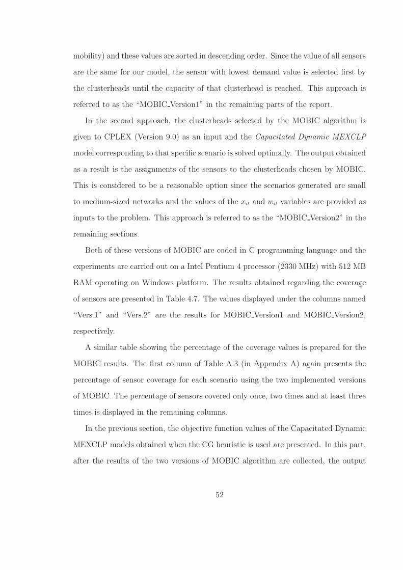
mobility) and these values are sorted in descending order. Since the value of all sensors

are the same for our model, the sensor with lowest demand value is selected first by

the clusterheads until the capacity of that clusterhead is reached. This approach is

referred to as the “MOBIC Version1” in the remaining parts of the report.

In the second approach, the clusterheads selected by the MOBIC algorithm is

given to CPLEX (Version 9.0) as an input and the Capacitated Dynamic MEXCLP

model corresponding to that specific scenario is solved optimally. The output obtained

as a result is the assignments of the sensors to the clusterheads chosen by MOBIC.

This is considered to be a reasonable option since the scenarios generated are small

to medium-sized networks and the values of the xit and wit variables are provided as

inputs to the problem. This approach is referred to as the “MOBIC Version2” in the

remaining sections.

Both of these versions of MOBIC are coded in C programming language and the

experiments are carried out on a Intel Pentium 4 processor (2330 MHz) with 512 MB

RAM operating on Windows platform. The results obtained regarding the coverage

of sensors are presented in Table 4.7. The values displayed under the columns named

“Vers.1” and “Vers.2” are the results for MOBIC Version1 and MOBIC Version2,

respectively.

A similar table showing the percentage of the coverage values is prepared for the

MOBIC results. The first column of Table A.3 (in Appendix A) again presents the

percentage of sensor coverage for each scenario using the two implemented versions

of MOBIC. The percentage of sensors covered only once, two times and at least three

times is displayed in the remaining columns.

In the previous section, the objective function values of the Capacitated Dynamic

MEXCLP models obtained when the CG heuristic is used are presented. In this part,

after the results of the two versions of MOBIC algorithm are collected, the output

52

of each scenario is used as an input and the corresponding objective function values

of the Capacitated Dynamic MEXCLP models are calculated. These values are then

compared with those of the CG heuristic to get an idea about how well MOBIC

performs in terms of maximizing the expected coverage while trying to maintain

stable clusters without an objective function. The values for Version 1 and Version 2

are given in Tables A.4 & A.5 of Appendix A, respectively.

When the results in Table 4.7 are examined, it is seen that Version 2 performs

better than Version 1 in terms of the coverage of sensors by the clusterheads. In

addition, according to the objective function values displayed in Tables A.4 and A.5,

Version 2 has higher values and it outperforms Version 1 by as much as 24.42% on

the average. This is an expected result since in the second version, CPLEX solves

the assignment problem optimally and maximizes the expected coverage.

4.2.1 Modified MOBIC Algorithm

In the original MOBIC algorithm, after a candidate clusterhead with the lowest rela-

tive mobility is chosen and some of the eligible sensors are assigned to it, all relative

mobility calculations are redone for the remaining clusterheads excluding the sensors

that have already been assigned. When the network size is large, this may result in

making the same calculations multiple times. Due to this reason, the original MO-

BIC algorithm is modified in a way that will determine the clusterheads after one

calculation of each relative mobility metric. In this approach, at the beginning of the

algorithm, the relative mobility values are calculated for each candidate clusterhead

taking into consideration all the sensors in the network. Then, these Mrel values are

ranked in increasing order and the smallest n (i.e. the number of clusterheads that

will be chosen in a scenario) candidates are chosen as the clusterheads. After the

clusterheads are determined, the sensors are assigned to them in two ways. These are

the same approaches that are used for the original MOBIC algorithm. In Version 1

53

of the modified algorithm, the sensor with smallest demand value is selected first. In

Version 2, CPLEX solves the Capacitated DMEXCLP model using the clusterhead

choices determined by the modified algorithm.

The two versions of the original MOBIC algorithm coded are modified and 64

scenarios are analyzed using the modified approach. The experiments are again car-

ried out on a Intel Pentium 4 processor (2330 MHz) with 512 MB RAM operating on

Windows platform. The results obtained are presented in Table 4.8. Table A.6 (in

Appendix A) shows the percentage of sensor coverage for each scenario. The percent-

age of sensors covered only once, two times and at least three times is also displayed

in the same table.

As a last step, the results obtained using the two versions of the modified MOBIC

algorithm are given as inputs for the objective function of the Capacitated DMEX-

CLP model and the corresponding objective function values are calculated for each

scenario. The values for Version 1 and Version 2 of the modified approach are given

in Tables A.7 & A.8 of Appendix A, respectively.

When the results of the modified MOBIC algorithm for Version 1 and 2 (Table 4.8)

are examined, it is seen that Version 2 is again superior. It results in higher number

of sensors covered in each scenario. In addition, the objective function values are

better for this version and it outperforms Version 1 by as much as 17.93% on the

average.

4.2.2 Discussion of the Results

During the numerical studies, it is observed that both the original MOBIC algorithm

and its modified version are solved very quickly (in two seconds, in the worst case) for

the network sizes chosen. The modified algorithm still requires less solution time (in

less than a second) when compared to original MOBIC as expected. However, when

the performance regarding the coverage of sensors is evaluated, the original MOBIC

54

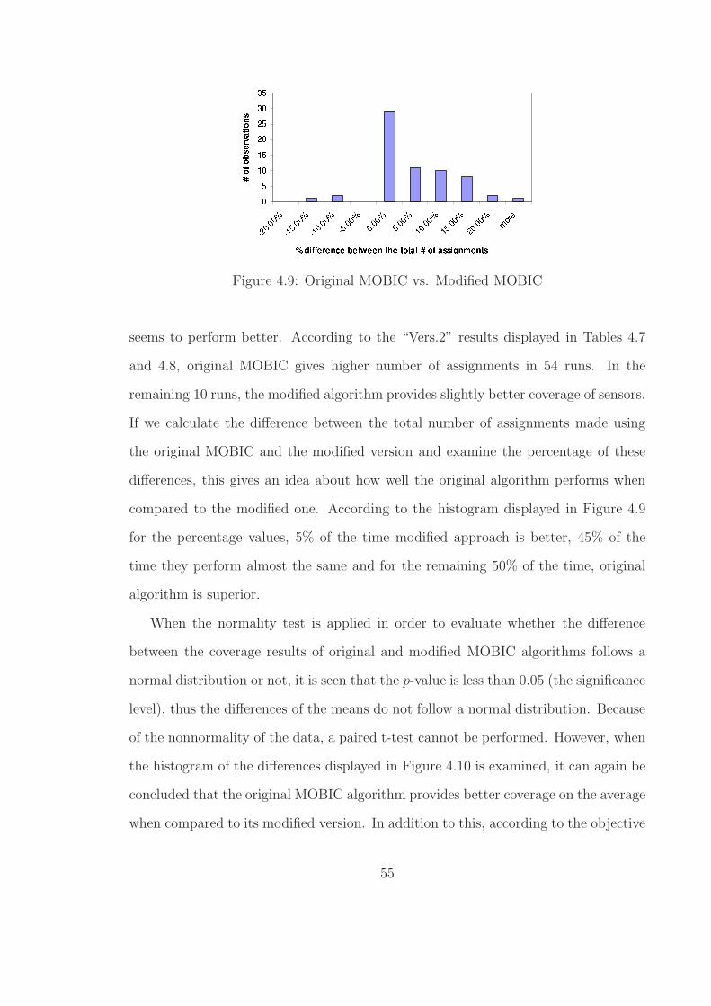
Figure 4.9: Original MOBIC vs. Modified MOBIC

seems to perform better. According to the “Vers.2” results displayed in Tables 4.7

and 4.8, original MOBIC gives higher number of assignments in 54 runs. In the

remaining 10 runs, the modified algorithm provides slightly better coverage of sensors.

If we calculate the difference between the total number of assignments made using

the original MOBIC and the modified version and examine the percentage of these

differences, this gives an idea about how well the original algorithm performs when

compared to the modified one. According to the histogram displayed in Figure 4.9

for the percentage values, 5% of the time modified approach is better, 45% of the

time they perform almost the same and for the remaining 50% of the time, original

algorithm is superior.

When the normality test is applied in order to evaluate whether the difference

between the coverage results of original and modified MOBIC algorithms follows a

normal distribution or not, it is seen that the p-value is less than 0.05 (the significance

level), thus the differences of the means do not follow a normal distribution. Because

of the nonnormality of the data, a paired t-test cannot be performed. However, when

the histogram of the differences displayed in Figure 4.10 is examined, it can again be

concluded that the original MOBIC algorithm provides better coverage on the average

when compared to its modified version. In addition to this, according to the objective

55

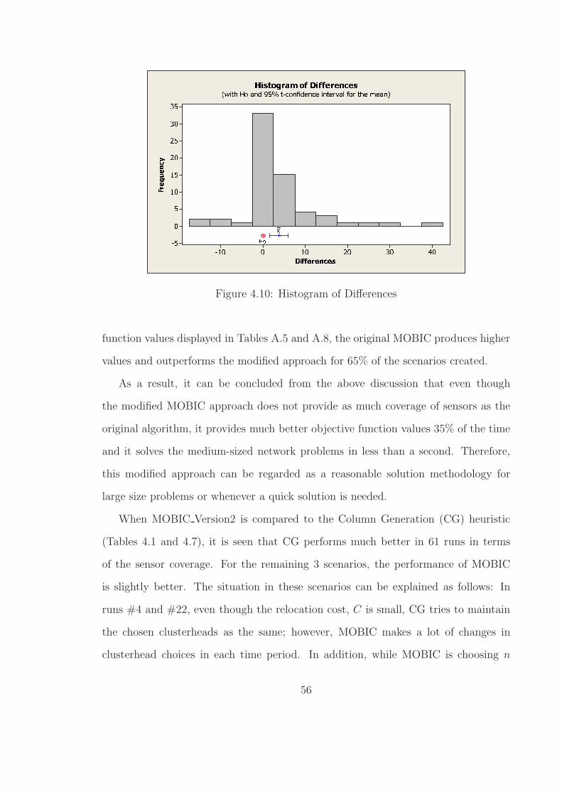
Figure 4.10: Histogram of Differences

function values displayed in Tables A.5 and A.8, the original MOBIC produces higher

values and outperforms the modified approach for 65% of the scenarios created.

As a result, it can be concluded from the above discussion that even though

the modified MOBIC approach does not provide as much coverage of sensors as the

original algorithm, it provides much better objective function values 35% of the time

and it solves the medium-sized network problems in less than a second. Therefore,

this modified approach can be regarded as a reasonable solution methodology for

large size problems or whenever a quick solution is needed.

When MOBIC Version2 is compared to the Column Generation (CG) heuristic

(Tables 4.1 and 4.7), it is seen that CG performs much better in 61 runs in terms

of the sensor coverage. For the remaining 3 scenarios, the performance of MOBIC

is slightly better. The situation in these scenarios can be explained as follows: In

runs #4 and #22, even though the relocation cost, C is small, CG tries to maintain

the chosen clusterheads as the same; however, MOBIC makes a lot of changes in

clusterhead choices in each time period. In addition, while MOBIC is choosing n

56

Figure 4.11: Number of CH Changes: CG vs. MOBIC

different clusterheads, it does not prefer multiple coverage of sensors. In run #33,

C=100, so CG does not change the chosen clusterheads during the periods. However,

MOBIC makes changes in the clusterheads selected. The graphs of Figure 4.11 present

the number of clusterhead changes made between two consecutive time periods. For

instance, the value for time period 1 shows the change in the choice of clusterheads

between periods 1 and 2. Even though the total number of sensor assignments is

higher when MOBIC is used, the objective function values of CG results corresponding

to these 3 scenarios (Tables A.2 and A.5) are much better and CG outperforms by

46.06% on the average for these scenarios.

4.3 Network Simulation Results

After the numerical studies regarding the coverage of sensors are completed, the

network models corresponding to each scenario are simulated using OPNET Modeler

57

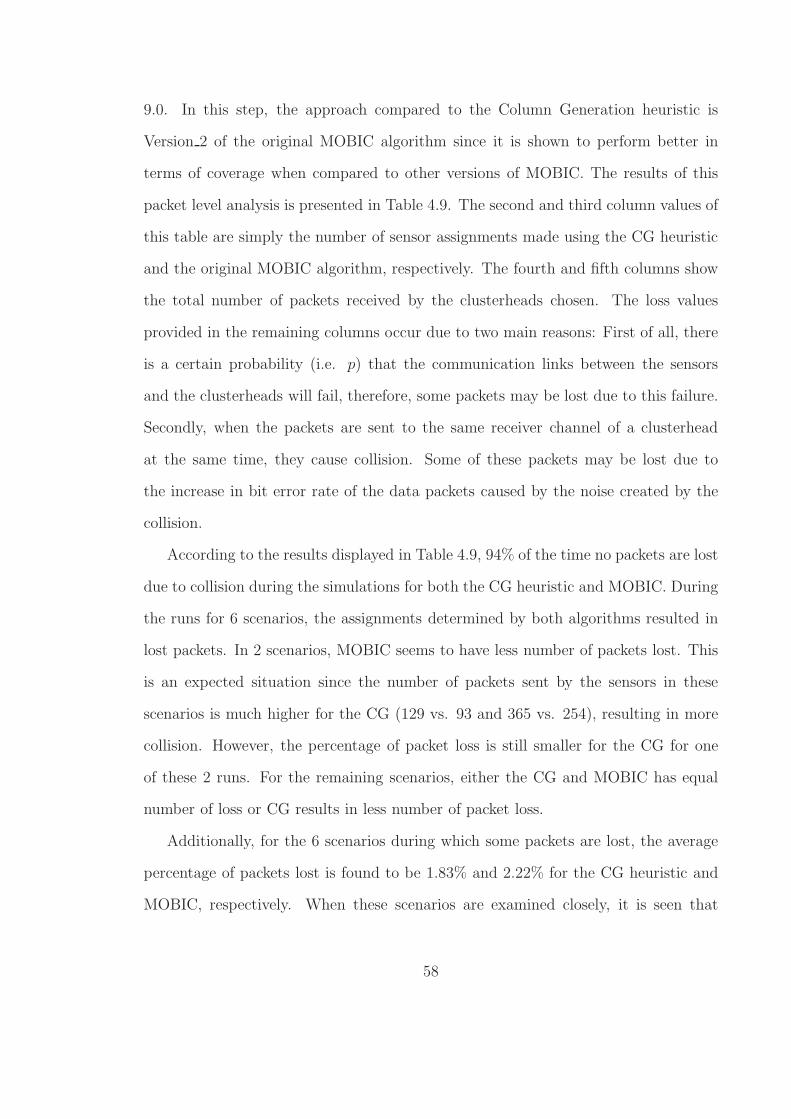
9.0. In this step, the approach compared to the Column Generation heuristic is

Version 2 of the original MOBIC algorithm since it is shown to perform better in

terms of coverage when compared to other versions of MOBIC. The results of this

packet level analysis is presented in Table 4.9. The second and third column values of

this table are simply the number of sensor assignments made using the CG heuristic

and the original MOBIC algorithm, respectively. The fourth and fifth columns show

the total number of packets received by the clusterheads chosen. The loss values

provided in the remaining columns occur due to two main reasons: First of all, there

is a certain probability (i.e. p) that the communication links between the sensors

and the clusterheads will fail, therefore, some packets may be lost due to this failure.

Secondly, when the packets are sent to the same receiver channel of a clusterhead

at the same time, they cause collision. Some of these packets may be lost due to

the increase in bit error rate of the data packets caused by the noise created by the

collision.

According to the results displayed in Table 4.9, 94% of the time no packets are lost

due to collision during the simulations for both the CG heuristic and MOBIC. During

the runs for 6 scenarios, the assignments determined by both algorithms resulted in

lost packets. In 2 scenarios, MOBIC seems to have less number of packets lost. This

is an expected situation since the number of packets sent by the sensors in these

scenarios is much higher for the CG (129 vs. 93 and 365 vs. 254), resulting in more

collision. However, the percentage of packet loss is still smaller for the CG for one

of these 2 runs. For the remaining scenarios, either the CG and MOBIC has equal

number of loss or CG results in less number of packet loss.

Additionally, for the 6 scenarios during which some packets are lost, the average

percentage of packets lost is found to be 1.83% and 2.22% for the CG heuristic and

MOBIC, respectively. When these scenarios are examined closely, it is seen that

58

there are certain factors that affect the level of packet loss during the simulations.

When runs 17&30 are compared, it is observed that as the clusterhead capacity (M)

increases, the packet loss due to collusion increases since more sensors are assigned to

the same clusterhead. Comparing runs 29&48, it can be said that as M increases and

the number of clusterheads chosen (n) decreases, the packet loss increases. Finally,

according to the runs 17&37, 17&47 and 30&37, as the coverage radius (D) increases,

the number of packet loss increases as expected.

A final observation that can be made from the results is that the percentage of

the packet loss due to the link failure does not exactly match the p level specified for

that specific scenario. This is an expected situation since the failures are incorporated

into the network models by generating random numbers and this procedure does not

guarantee that p level. It is also obvious that as p decreases, total number of packets

lost due to p decreases as well.

59

Performance MetricsTotal # Total # Total #

Run Total # of of single of double of at leastNumber assignments coverage coverage triple coverage

1 68 25 19 242 393 77 105 2113 80 50 17 134 60 23 17 205 85 65 20 06 68 25 19 247 164 104 60 08 48 37 9 29 151 93 51 710 60 50 10 011 81 51 21 912 162 118 40 413 89 65 20 414 225 36 60 12915 50 32 13 516 146 97 48 117 129 125 4 018 124 90 33 119 76 43 22 1120 178 79 44 5521 172 42 54 7622 52 8 17 2723 164 46 59 5924 89 65 20 425 177 75 64 3826 60 50 10 027 85 25 21 3928 183 47 38 9829 199 51 100 4830 321 153 104 6431 95 66 29 032 81 50 31 033 25 17 5 334 89 65 20 435 354 137 146 7136 49 37 7 537 326 235 87 438 56 32 16 8

60

Performance MetricsTotal # Total # Total #

Run Total # of of single of double of at leastNumber assignments coverage coverage triple coverage

39 89 40 29 2040 50 32 13 541 85 65 20 042 91 32 26 3343 80 50 17 1344 158 83 27 4845 281 215 53 1346 62 42 20 047 174 65 78 3148 365 214 100 5149 181 128 44 950 89 40 29 2051 54 34 19 152 75 45 23 753 159 72 55 3254 68 50 18 055 76 48 17 1156 162 118 40 457 98 25 35 3858 99 72 22 559 293 236 57 060 171 132 39 061 167 106 51 1062 225 36 60 12963 103 103 0 064 81 51 21 9

Table 4.1: Coverage Results for the Column Generation Heuristic

61

Run % of sensors % of single % of double % of at leastNumber covered coverage coverage triple coverage

1 74.73 36.76 27.94 35.292 99.75 19.59 26.72 53.693 98.77 62.50 21.25 16.254 89.55 38.33 28.33 33.335 100.00 76.47 23.53 0.006 74.73 36.76 27.94 35.297 57.54 63.41 36.59 0.008 59.26 77.08 18.75 4.179 98.05 61.59 33.77 4.6410 100.00 83.33 16.67 0.0011 100.00 62.96 25.93 11.1112 98.78 72.84 24.69 2.4713 98.89 73.03 22.47 4.4914 58.59 16.00 26.67 57.3315 55.56 64.00 26.00 10.0016 100.00 66.44 32.88 0.6817 96.99 96.90 3.10 0.0018 94.66 72.58 26.61 0.8119 84.44 56.58 28.95 14.4720 97.27 44.38 24.72 30.9021 100.00 24.42 31.40 44.1922 57.14 15.38 32.69 51.9223 88.65 28.05 35.98 35.9824 98.89 73.03 22.47 4.4925 98.88 42.37 36.16 21.4726 100.00 83.33 16.67 0.0027 100.00 29.41 24.71 45.8828 100.00 25.68 20.77 53.5529 100.00 25.63 50.25 24.1230 99.07 47.66 32.40 19.9431 55.88 69.47 30.53 0.0032 56.25 61.73 38.27 0.0033 39.06 68.00 20.00 12.0034 98.89 73.03 22.47 4.4935 100.00 38.70 41.24 20.0636 60.49 75.51 14.29 10.2037 92.09 72.09 26.69 1.2338 46.67 57.14 28.57 14.2939 100.00 44.94 32.58 22.4740 55.56 64.00 26.00 10.00

62

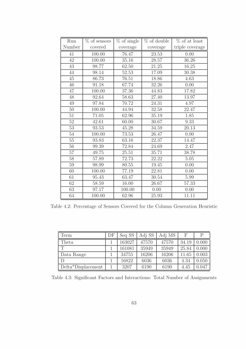
Run % of sensors % of single % of double % of at leastNumber covered coverage coverage triple coverage

41 100.00 76.47 23.53 0.0042 100.00 35.16 28.57 36.2643 98.77 62.50 21.25 16.2544 98.14 52.53 17.09 30.3845 86.73 76.51 18.86 4.6346 91.18 67.74 32.26 0.0047 100.00 37.36 44.83 17.8248 92.64 58.63 27.40 13.9749 97.84 70.72 24.31 4.9750 100.00 44.94 32.58 22.4751 71.05 62.96 35.19 1.8552 42.61 60.00 30.67 9.3353 93.53 45.28 34.59 20.1354 100.00 73.53 26.47 0.0055 93.83 63.16 22.37 14.4756 99.39 72.84 24.69 2.4757 49.75 25.51 35.71 38.7858 57.89 72.73 22.22 5.0559 98.99 80.55 19.45 0.0060 100.00 77.19 22.81 0.0061 95.43 63.47 30.54 5.9962 58.59 16.00 26.67 57.3363 97.17 100.00 0.00 0.0064 100.00 62.96 25.93 11.11

Table 4.2: Percentage of Sensors Covered for the Column Generation Heuristic

Term DF Seq SS Adj SS Adj MS F P

Theta 1 163027 47570 47570 34.19 0.000T 1 161081 35949 35949 25.84 0.000Data Range 1 34755 16206 16206 11.65 0.003D 1 16822 6036 6036 4.34 0.050Delta*Displacement 1 3207 6190 6190 4.45 0.047

Table 4.3: Significant Factors and Interactions: Total Number of Assignments

63

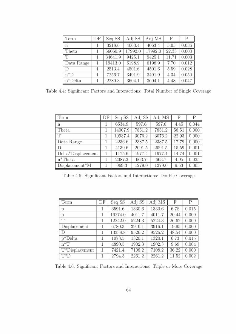
Term DF Seq SS Adj SS Adj MS F P

n 1 3218.6 4063.4 4063.4 5.05 0.036Theta 1 56060.9 17992.0 17992.0 22.35 0.000T 1 34641.9 9425.1 9425.1 11.71 0.003Data Range 1 19413.0 6198.9 6198.9 7.70 0.012D 1 2513.4 4501.6 4501.6 5.59 0.028n*D 1 7256.7 3491.9 3491.9 4.34 0.050p*Delta 1 2280.3 3604.1 3604.1 4.48 0.047

Table 4.4: Significant Factors and Interactions: Total Number of Single Coverage

Term DF Seq SS Adj SS Adj MS F P

n 1 6534.9 597.6 597.6 4.45 0.044Theta 1 14007.9 7851.2 7851.2 58.51 0.000T 1 10937.4 3076.2 3076.2 22.93 0.000Data Range 1 2236.6 2387.5 2387.5 17.79 0.000D 1 4139.6 2091.5 2091.5 15.59 0.001Delta*Displacement 1 1175.6 1977.4 1977.4 14.74 0.001n*Theta 1 2087.3 663.7 663.7 4.95 0.035Displacement*M 1 969.3 1279.0 1279.0 9.53 0.005

Table 4.5: Significant Factors and Interactions: Double Coverage

Term DF Seq SS Adj SS Adj MS F P

p 1 3591.6 1330.6 1330.6 6.78 0.015n 1 16274.0 4011.7 4011.7 20.44 0.000T 1 12242.0 5224.3 5224.3 26.62 0.000Displacement 1 6780.3 3916.1 3916.1 19.95 0.000D 1 13338.8 9526.2 9526.2 48.54 0.000p*Delta 1 1073.5 1320.1 1320.1 6.73 0.015n*T 1 4890.5 1902.3 1902.3 9.69 0.004T*Displacement 1 7421.4 7108.2 7108.2 36.22 0.000T*D 1 2794.3 2261.2 2261.2 11.52 0.002

Table 4.6: Significant Factors and Interactions: Triple or More Coverage

64

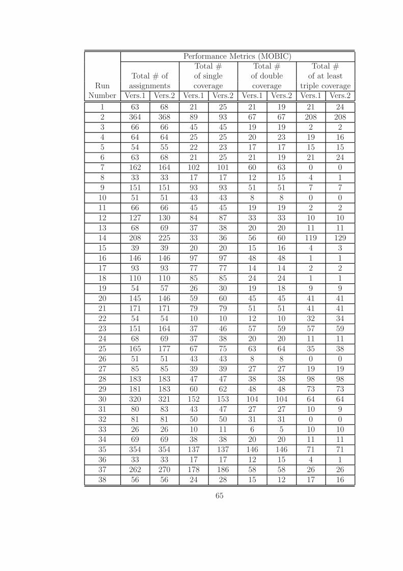
Performance Metrics (MOBIC)Total # Total # Total #

Total # of of single of double of at leastRun assignments coverage coverage triple coverage

Number Vers.1 Vers.2 Vers.1 Vers.2 Vers.1 Vers.2 Vers.1 Vers.2

1 63 68 21 25 21 19 21 242 364 368 89 93 67 67 208 2083 66 66 45 45 19 19 2 24 64 64 25 25 20 23 19 165 54 55 22 23 17 17 15 156 63 68 21 25 21 19 21 247 162 164 102 101 60 63 0 08 33 33 17 17 12 15 4 19 151 151 93 93 51 51 7 710 51 51 43 43 8 8 0 011 66 66 45 45 19 19 2 212 127 130 84 87 33 33 10 1013 68 69 37 38 20 20 11 1114 208 225 33 36 56 60 119 12915 39 39 20 20 15 16 4 316 146 146 97 97 48 48 1 117 93 93 77 77 14 14 2 218 110 110 85 85 24 24 1 119 54 57 26 30 19 18 9 920 145 146 59 60 45 45 41 4121 171 171 79 79 51 51 41 4122 54 54 10 10 12 10 32 3423 151 164 37 46 57 59 57 5924 68 69 37 38 20 20 11 1125 165 177 67 75 63 64 35 3826 51 51 43 43 8 8 0 027 85 85 39 39 27 27 19 1928 183 183 47 47 38 38 98 9829 181 183 60 62 48 48 73 7330 320 321 152 153 104 104 64 6431 80 83 43 47 27 27 10 932 81 81 50 50 31 31 0 033 26 26 10 11 6 5 10 1034 69 69 38 38 20 20 11 1135 354 354 137 137 146 146 71 7136 33 33 17 17 12 15 4 137 262 270 178 186 58 58 26 2638 56 56 24 28 15 12 17 16

65

Performance Metrics (MOBIC)Total # Total # Total #

Total # of of single of double of at leastRun assignments coverage coverage triple coverage

Number Vers.1 Vers.2 Vers.1 Vers.2 Vers.1 Vers.2 Vers.1 Vers.2

39 84 89 36 40 29 29 19 2040 39 39 20 20 15 16 4 341 56 56 25 25 16 16 15 1542 91 91 32 32 26 26 33 3343 66 66 45 45 19 19 2 244 157 157 74 74 48 48 35 3545 216 216 147 147 51 51 18 1846 47 47 29 29 9 9 9 947 174 174 65 65 78 78 31 3148 253 254 82 83 83 83 88 8849 102 102 46 46 32 32 24 2450 89 89 40 40 29 29 20 2051 52 54 35 34 16 19 1 152 69 71 32 32 32 34 5 553 123 123 67 67 31 31 25 2554 68 68 50 50 18 18 0 055 49 52 26 29 18 18 5 556 127 130 84 87 33 33 10 1057 74 85 27 23 26 33 21 2958 63 63 32 32 22 30 9 159 225 225 178 178 41 41 6 660 136 136 93 93 40 40 3 361 139 139 90 90 37 37 12 1262 208 225 33 36 56 60 119 12963 46 46 36 36 8 8 2 264 66 66 45 45 19 19 2 2

Table 4.7: Coverage Results for the Original MOBIC Algorithm

66

Performance Metrics (Modified MOBIC)Total # Total # Total #

Total # of of single of double of at leastRun assignments coverage coverage triple coverage

Number Vers.1 Vers.2 Vers.1 Vers.2 Vers.1 Vers.2 Vers.1 Vers.2

1 63 68 21 25 21 19 21 242 338 342 87 90 73 74 178 1783 59 59 39 39 18 18 2 24 56 56 15 14 23 25 18 175 56 56 24 24 19 19 13 136 63 68 21 25 21 19 21 247 162 164 102 103 60 61 0 08 31 32 19 19 10 13 2 09 151 151 93 93 51 51 7 710 48 48 39 39 9 9 0 011 59 59 39 39 18 18 2 212 142 143 110 111 28 28 4 413 63 65 36 38 20 20 7 714 208 225 33 36 56 60 119 12915 39 39 22 22 10 12 7 516 146 146 97 97 48 48 1 117 89 89 74 74 14 14 1 118 104 104 79 79 25 25 0 019 54 56 30 32 17 17 7 720 139 141 50 52 49 49 40 4021 157 157 49 49 32 32 76 7622 52 53 11 11 16 17 25 2523 151 164 37 46 57 59 57 5924 63 65 36 38 20 20 7 725 165 177 67 75 63 64 35 3826 48 48 39 39 9 9 0 027 75 75 19 19 15 15 41 4128 183 183 47 47 38 38 98 9829 162 166 59 62 43 44 60 6030 320 321 152 153 104 104 64 6431 82 86 50 53 28 29 4 432 81 81 50 50 31 31 0 033 27 27 11 11 7 6 9 1034 65 65 38 38 20 20 7 735 354 354 137 137 146 146 71 7136 31 32 19 19 10 13 2 037 272 278 204 210 64 64 4 438 57 57 29 30 15 13 13 14

67

Performance Metrics (Modified MOBIC)Total # Total # Total #

Total # of of single of double of at leastRun assignments coverage coverage triple coverage

Number Vers.1 Vers.2 Vers.1 Vers.2 Vers.1 Vers.2 Vers.1 Vers.2

39 84 89 36 40 29 29 19 2040 39 39 22 22 10 12 7 541 56 56 24 24 19 19 13 1342 91 91 32 32 26 26 33 3343 59 59 39 39 18 18 2 244 141 141 57 57 41 41 43 4345 209 209 151 151 55 55 3 346 40 40 28 28 6 6 6 647 174 174 65 65 78 78 31 3148 242 243 93 94 57 57 92 9249 99 99 49 49 22 22 28 2850 89 89 40 40 29 29 20 2051 52 54 35 34 16 19 1 152 70 72 38 39 26 27 6 653 114 114 47 47 43 43 24 2454 68 68 50 50 18 18 0 055 48 51 30 33 16 16 2 256 142 143 110 111 28 28 4 457 77 87 35 36 13 19 29 3258 61 62 34 34 20 28 7 059 184 184 123 123 41 41 20 2060 114 114 73 73 34 34 7 761 109 109 68 68 25 25 16 1662 208 225 33 36 56 60 119 12963 54 54 48 48 6 6 0 064 59 59 39 39 18 18 2 2

Table 4.8: Coverage Results for the Modified MOBIC Algorithm

68

Total # Total # Total # of Total # ofof packets of packets packets lost packets lost

Run sent received due to p due to collisionNumber CG MOBIC CG MOBIC CG MOBIC CG MOBIC

1 68 68 54 53 14 15 0 02 393 368 120 101 273 267 0 03 80 66 62 52 18 14 0 04 60 64 12 21 48 43 0 05 85 55 65 43 20 12 0 06 68 68 19 19 49 49 0 07 164 164 42 51 122 113 0 08 48 33 38 25 10 8 0 09 151 151 43 43 108 108 0 010 60 51 46 40 14 11 0 011 81 66 63 52 18 14 0 012 162 130 46 38 116 92 0 013 89 69 68 55 21 14 0 014 225 225 176 178 49 47 0 015 50 39 40 31 10 8 0 016 146 146 39 39 107 107 0 017 129 93 93 72 33 21 3 018 124 110 89 84 35 26 0 019 76 57 58 45 18 12 0 020 178 146 46 38 132 108 0 021 172 171 138 136 34 35 0 022 52 54 39 41 13 13 0 023 164 164 50 50 114 114 0 024 89 69 69 54 20 15 0 025 177 177 47 47 130 130 0 026 60 51 22 15 38 36 0 027 85 85 23 23 62 62 0 028 183 183 141 141 42 42 0 029 199 183 146 140 51 41 2 230 321 321 257 254 62 63 2 431 95 83 71 66 24 17 0 032 81 81 63 63 18 18 0 033 25 26 20 21 5 5 0 034 89 69 68 55 21 14 0 035 354 354 111 111 243 243 0 036 49 33 16 10 33 23 0 037 326 270 253 198 66 62 7 1038 56 56 12 18 44 38 0 039 89 89 68 68 21 21 0 0

69

Total # Total # Total # of Total # ofof packets of packets packets lost packets lost

Run sent received due to p due to collisionNumber CG MOBIC CG MOBIC CG MOBIC CG MOBIC

40 50 39 40 30 10 9 0 041 85 56 65 43 20 13 0 042 91 91 30 27 61 64 0 043 80 66 26 18 54 48 0 044 158 157 44 43 114 114 0 045 281 216 83 60 198 156 0 046 62 47 21 12 41 35 0 047 174 174 126 128 43 41 5 548 365 254 277 184 74 59 14 1149 181 102 57 27 124 75 0 050 89 89 68 70 21 19 0 051 54 54 20 17 34 37 0 052 75 71 61 57 14 14 0 053 159 123 45 36 114 87 0 054 68 68 53 53 15 15 0 055 76 52 60 41 16 11 0 056 162 130 122 100 40 27 0 357 98 85 29 26 69 59 0 058 99 63 78 50 21 13 0 059 293 225 236 170 57 55 0 060 171 136 122 107 49 29 0 061 167 139 52 41 115 98 0 062 225 225 61 61 164 164 0 063 103 46 82 36 21 10 0 064 81 66 63 51 18 15 0 0

Table 4.9: Results for the Packet Level Analysis

70

Chapter 5

Conclusions

This work was an attempt towards a comprehensive performance evaluation of a

mathematical programming based clustering algorithm for mobile, wireless ad hoc

networks. We dealt with a communication network problem of finding optimal lo-

cations of clusterheads for collecting data from sensors spread over a geographically

dispersed area for the purpose of data fusion. Mishra [19] developed the mathematical

model for the Capacitated DMEXCLP incorporating issues of link failure and mobil-

ity of the system entities (i.e. sensors) and proposed a Column Generation heuristic

used in conjunction with two greedy heuristics as the solution methodology. As a

result of the numerical studies, it is concluded that this approach solves the problem

with a reasonable accuracy, efficiently.

This approach is compared with the MOBIC clustering algorithm [4] proposed in

the literature. First of all, the performance regarding the coverage of sensors in the

network is evaluated. Secondly, a packet level simulation model is constructed using

OPNET Modeler 9.0 and the network models corresponding to the scenarios gener-

ated are tested to validate the performance of the clusters formed by the clustering

algorithms under realistic (simulated) conditions.

As a result of numerical studies regarding the coverage level of sensors by the

clusterheads, it is concluded that Version 2 of the MOBIC algorithms is superior over

71

Version 1 as expected. When these versions of the original MOBIC and the modified

approach are compared, it is seen that 5% of the time the modified algorithm is better

and for the remaining 95%, the original algorithm performs either the same or better.

Finally, the CG heuristic performs much better in terms of sensor coverage when

compared to the Version 2 of the original MOBIC algorithm. During 3 scenarios out

of 64, MOBIC provides slightly better coverage, however when the objective function

values of the Capacitated DMEXCLP model are compared for these scenarios, it is

seen that the CG heuristic outperforms by 46.06%.

As a result of the packet level analysis performed using OPNET, it is seen that

only a small percentage of packets sent by the sensors is lost due to the probability

of link failure or the collision of packets transmitted to the same receiver channel of

a clusterhead. According to the results, 94% of the time no packets are lost due to

collision during the simulations for both the CG heuristic and MOBIC. In addition, for

the 6 scenarios during which some packets are lost, the average percentage of packets

lost is found to be 1.83% and 2.22% for the CG heuristic and MOBIC, respectively.

72

Appendix A

Numerical Results

Run 1 91 Run 17 133 Run 33 64 Run 49 185Run 2 394 Run 18 131 Run 34 90 Run 50 89Run 3 81 Run 19 90 Run 35 354 Run 51 76Run 4 67 Run 20 183 Run 36 81 Run 52 176Run 5 85 Run 21 172 Run 37 354 Run 53 170Run 6 91 Run 22 91 Run 38 120 Run 54 68Run 7 285 Run 23 185 Run 39 89 Run 55 81Run 8 81 Run 24 90 Run 40 90 Run 56 163Run 9 154 Run 25 179 Run 41 85 Run 57 197Run 10 60 Run 26 60 Run 42 91 Run 58 171Run 11 81 Run 27 85 Run 43 81 Run 59 296Run 12 164 Run 28 183 Run 44 161 Run 60 171Run 13 90 Run 29 199 Run 45 324 Run 61 175Run 14 384 Run 30 324 Run 46 68 Run 62 384Run 15 90 Run 31 170 Run 47 174 Run 63 106Run 16 146 Run 32 144 Run 48 394 Run 64 81

Table A.1: Maximum Number of Assignments Possible for Each Scenario

73

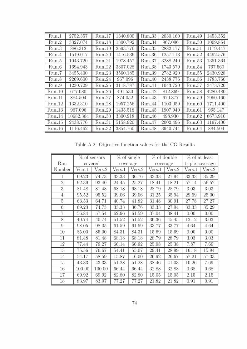
Run 1 2752.357 Run 17 1340.800 Run 33 2030.160 Run 49 1453.352Run 2 3327.074 Run 18 1300.792 Run 34 967.096 Run 50 1009.864Run 3 886.312 Run 19 2593.776 Run 35 2882.177 Run 51 1179.447Run 4 1519.017 Run 20 1416.536 Run 36 1257.113 Run 52 4492.576Run 5 1043.720 Run 21 1978.457 Run 37 3288.240 Run 53 1351.364Run 6 1694.943 Run 22 3307.028 Run 38 1743.579 Run 54 767.560Run 7 3455.400 Run 23 3560.185 Run 39 2782.920 Run 55 2430.928Run 8 2269.600 Run 24 967.096 Run 40 2438.776 Run 56 1783.760Run 9 1230.729 Run 25 3118.787 Run 41 1043.720 Run 57 3473.720Run 10 677.080 Run 26 491.530 Run 42 812.869 Run 58 4280.480Run 11 884.504 Run 27 874.052 Run 43 670.377 Run 59 2950.160Run 12 1332.310 Run 28 1957.256 Run 44 1103.059 Run 60 1711.400Run 13 967.096 Run 29 1435.518 Run 45 1907.940 Run 61 965.147Run 14 10682.364 Run 30 3300.918 Run 46 498.930 Run 62 6673.910Run 15 2438.776 Run 31 5158.920 Run 47 2002.496 Run 63 1197.400Run 16 1116.462 Run 32 3854.760 Run 48 3940.744 Run 64 884.504

Table A.2: Objective function values for the CG Results

% of sensors % of single % of double % of at leastRun covered coverage coverage triple coverage

Number Vers.1 Vers.2 Vers.1 Vers.2 Vers.1 Vers.2 Vers.1 Vers.2

1 69.23 74.73 33.33 36.76 33.33 27.94 33.33 35.292 92.39 93.40 24.45 25.27 18.41 18.21 57.14 56.523 81.48 81.48 68.18 68.18 28.79 28.79 3.03 3.034 95.52 95.52 39.06 39.06 31.25 35.94 29.69 25.005 63.53 64.71 40.74 41.82 31.48 30.91 27.78 27.276 69.23 74.73 33.33 36.76 33.33 27.94 33.33 35.297 56.84 57.54 62.96 61.59 37.04 38.41 0.00 0.008 40.74 40.74 51.52 51.52 36.36 45.45 12.12 3.039 98.05 98.05 61.59 61.59 33.77 33.77 4.64 4.6410 85.00 85.00 84.31 84.31 15.69 15.69 0.00 0.0011 81.48 81.48 68.18 68.18 28.79 28.79 3.03 3.0312 77.44 79.27 66.14 66.92 25.98 25.38 7.87 7.6913 75.56 76.67 54.41 55.07 29.41 28.99 16.18 15.9414 54.17 58.59 15.87 16.00 26.92 26.67 57.21 57.3315 43.33 43.33 51.28 51.28 38.46 41.03 10.26 7.6916 100.00 100.00 66.44 66.44 32.88 32.88 0.68 0.6817 69.92 69.92 82.80 82.80 15.05 15.05 2.15 2.1518 83.97 83.97 77.27 77.27 21.82 21.82 0.91 0.91

74

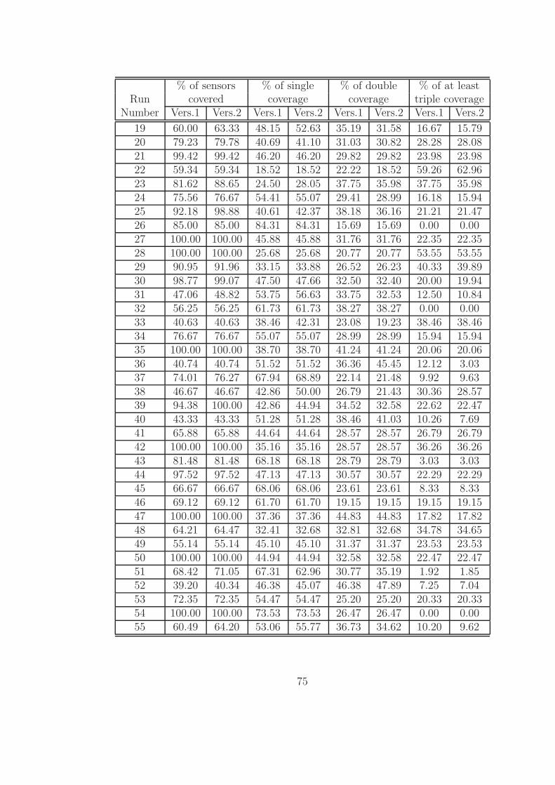
% of sensors % of single % of double % of at leastRun covered coverage coverage triple coverage

Number Vers.1 Vers.2 Vers.1 Vers.2 Vers.1 Vers.2 Vers.1 Vers.2

19 60.00 63.33 48.15 52.63 35.19 31.58 16.67 15.7920 79.23 79.78 40.69 41.10 31.03 30.82 28.28 28.0821 99.42 99.42 46.20 46.20 29.82 29.82 23.98 23.9822 59.34 59.34 18.52 18.52 22.22 18.52 59.26 62.9623 81.62 88.65 24.50 28.05 37.75 35.98 37.75 35.9824 75.56 76.67 54.41 55.07 29.41 28.99 16.18 15.9425 92.18 98.88 40.61 42.37 38.18 36.16 21.21 21.4726 85.00 85.00 84.31 84.31 15.69 15.69 0.00 0.0027 100.00 100.00 45.88 45.88 31.76 31.76 22.35 22.3528 100.00 100.00 25.68 25.68 20.77 20.77 53.55 53.5529 90.95 91.96 33.15 33.88 26.52 26.23 40.33 39.8930 98.77 99.07 47.50 47.66 32.50 32.40 20.00 19.9431 47.06 48.82 53.75 56.63 33.75 32.53 12.50 10.8432 56.25 56.25 61.73 61.73 38.27 38.27 0.00 0.0033 40.63 40.63 38.46 42.31 23.08 19.23 38.46 38.4634 76.67 76.67 55.07 55.07 28.99 28.99 15.94 15.9435 100.00 100.00 38.70 38.70 41.24 41.24 20.06 20.0636 40.74 40.74 51.52 51.52 36.36 45.45 12.12 3.0337 74.01 76.27 67.94 68.89 22.14 21.48 9.92 9.6338 46.67 46.67 42.86 50.00 26.79 21.43 30.36 28.5739 94.38 100.00 42.86 44.94 34.52 32.58 22.62 22.4740 43.33 43.33 51.28 51.28 38.46 41.03 10.26 7.6941 65.88 65.88 44.64 44.64 28.57 28.57 26.79 26.7942 100.00 100.00 35.16 35.16 28.57 28.57 36.26 36.2643 81.48 81.48 68.18 68.18 28.79 28.79 3.03 3.0344 97.52 97.52 47.13 47.13 30.57 30.57 22.29 22.2945 66.67 66.67 68.06 68.06 23.61 23.61 8.33 8.3346 69.12 69.12 61.70 61.70 19.15 19.15 19.15 19.1547 100.00 100.00 37.36 37.36 44.83 44.83 17.82 17.8248 64.21 64.47 32.41 32.68 32.81 32.68 34.78 34.6549 55.14 55.14 45.10 45.10 31.37 31.37 23.53 23.5350 100.00 100.00 44.94 44.94 32.58 32.58 22.47 22.4751 68.42 71.05 67.31 62.96 30.77 35.19 1.92 1.8552 39.20 40.34 46.38 45.07 46.38 47.89 7.25 7.0453 72.35 72.35 54.47 54.47 25.20 25.20 20.33 20.3354 100.00 100.00 73.53 73.53 26.47 26.47 0.00 0.0055 60.49 64.20 53.06 55.77 36.73 34.62 10.20 9.62

75

% of sensors % of single % of double % of at leastRun covered coverage coverage triple coverage

Number Vers.1 Vers.2 Vers.1 Vers.2 Vers.1 Vers.2 Vers.1 Vers.2

56 77.91 79.75 66.14 66.92 25.98 25.38 7.87 7.6957 37.56 43.15 36.49 27.06 35.14 38.82 28.38 34.1258 36.84 36.84 50.79 50.79 34.92 47.62 14.29 1.5959 76.01 76.01 79.11 79.11 18.22 18.22 2.67 2.6760 79.53 79.53 68.38 68.38 29.41 29.41 2.21 2.2161 79.43 79.43 64.75 64.75 26.62 26.62 8.63 8.6362 54.17 58.59 15.87 16.00 26.92 26.67 57.21 57.3363 43.40 43.40 78.26 78.26 17.39 17.39 4.35 4.3564 81.48 81.48 68.18 68.18 28.79 28.79 3.03 3.03

Table A.3: Percentage of Sensors Covered for the MOBIC Algorithm

Run 1 1532.168 Run 17 -211.816 Run 33 -110.760 Run 49 641.401Run 2 2406.868 Run 18 1021.312 Run 34 641.288 Run 50 1009.864Run 3 355.408 Run 19 1460.168 Run 35 2882.177 Run 51 623.686Run 4 1178.387 Run 20 838.796 Run 36 474.460 Run 52 1086.752Run 5 574.320 Run 21 1817.443 Run 37 2335.280 Run 53 -798.787Run 6 977.900 Run 22 1502.510 Run 38 858.087 Run 54 767.560Run 7 1773.590 Run 23 2710.155 Run 39 2598.304 Run 55 1448.960Run 8 780.960 Run 24 -631.712 Run 40 808.080 Run 56 1160.152Run 9 1221.729 Run 25 2801.939 Run 41 574.080 Run 57 932.743Run 10 534.120 Run 26 -175.030 Run 42 812.869 Run 58 876.560Run 11 715.408 Run 27 309.871 Run 43 510.818 Run 59 1879.368Run 12 -410.473 Run 28 1957.256 Run 44 735.211 Run 60 1350.272Run 13 628.288 Run 29 -2153.121 Run 45 1235.876 Run 61 -3312.257Run 14 3950.447 Run 30 3163.918 Run 46 89.297 Run 62 2832.294Run 15 -91.920 Run 31 -186.112 Run 47 2002.496 Run 63 300.776Run 16 1116.462 Run 32 1638.600 Run 48 -2542.400 Run 64 715.408

Table A.4: Objective function values for MOBIC Version1 Results

76

Run 1 2752.357 Run 17 -211.816 Run 33 30.040 Run 49 641.401Run 2 2439.768 Run 18 1021.312 Run 34 641.288 Run 50 1009.864Run 3 355.408 Run 19 1859.968 Run 35 2882.177 Run 51 1179.447Run 4 1218.576 Run 20 846.796 Run 36 856.120 Run 52 3382.928Run 5 587.320 Run 21 1817.443 Run 37 2447.280 Run 53 -798.787Run 6 1694.943 Run 22 2650.006 Run 38 1052.803 Run 54 767.560Run 7 3455.400 Run 23 3560.185 Run 39 2782.920 Run 55 1814.040Run 8 1684.320 Run 24 -618.712 Run 40 1796.240 Run 56 1207.152Run 9 1230.729 Run 25 3118.787 Run 41 574.080 Run 57 2486.201Run 10 534.120 Run 26 -175.030 Run 42 812.869 Run 58 2541.520Run 11 715.408 Run 27 309.871 Run 43 510.818 Run 59 1879.368Run 12 -383.473 Run 28 1957.256 Run 44 735.211 Run 60 1350.272Run 13 641.288 Run 29 -2121.521 Run 45 1235.876 Run 61 -3312.257Run 14 10682.364 Run 30 3300.918 Run 46 89.297 Run 62 6673.910Run 15 896.240 Run 31 1033.928 Run 47 2002.496 Run 63 300.776Run 16 1116.462 Run 32 3854.760 Run 48 -2530.200 Run 64 715.408

Table A.5: Objective function values for MOBIC Version2 Results

% of sensors % of single % of double % of at leastRun covered coverage coverage triple coverage

Number Vers.1 Vers.2 Vers.1 Vers.2 Vers.1 Vers.2 Vers.1 Vers.2

1 69.23 74.73 33.33 36.76 33.33 27.94 33.33 35.292 85.79 86.80 25.74 26.32 21.60 21.64 52.66 52.053 72.84 72.84 66.10 66.10 30.51 30.51 3.39 3.394 83.58 83.58 26.79 25.00 41.07 44.64 32.14 30.365 65.88 65.88 42.86 42.86 33.93 33.93 23.21 23.216 69.23 74.73 33.33 36.76 33.33 27.94 33.33 35.297 56.84 57.54 62.96 62.80 37.04 37.20 0.00 0.008 38.27 39.51 61.29 59.38 32.26 40.63 6.45 0.009 98.05 98.05 61.59 61.59 33.77 33.77 4.64 4.6410 80.00 80.00 81.25 81.25 18.75 18.75 0.00 0.0011 72.84 72.84 66.10 66.10 30.51 30.51 3.39 3.3912 86.59 87.20 77.46 77.62 19.72 19.58 2.82 2.8013 70.00 72.22 57.14 58.46 31.75 30.77 11.11 10.7714 54.17 58.59 15.87 16.00 26.92 26.67 57.21 57.3315 43.33 43.33 56.41 56.41 25.64 30.77 17.95 12.8216 100.00 100.00 66.44 66.44 32.88 32.88 0.68 0.6817 66.92 66.92 83.15 83.15 15.73 15.73 1.12 1.1218 79.39 79.39 75.96 75.96 24.04 24.04 0.00 0.00

77

% of sensors % of single % of double % of at leastRun covered coverage coverage triple coverage

Number Vers.1 Vers.2 Vers.1 Vers.2 Vers.1 Vers.2 Vers.1 Vers.2

19 60.00 62.22 55.56 57.14 31.48 30.36 12.96 12.5020 75.96 77.05 35.97 36.88 35.25 34.75 28.78 28.3721 91.28 91.28 31.21 31.21 20.38 20.38 48.41 48.4122 57.14 58.24 21.15 20.75 30.77 32.08 48.08 47.1723 81.62 88.65 24.50 28.05 37.75 35.98 37.75 35.9824 70.00 72.22 57.14 58.46 31.75 30.77 11.11 10.7725 92.18 98.88 40.61 42.37 38.18 36.16 21.21 21.4726 80.00 80.00 81.25 81.25 18.75 18.75 0.00 0.0027 88.24 88.24 25.33 25.33 20.00 20.00 54.67 54.6728 100.00 100.00 25.68 25.68 20.77 20.77 53.55 53.5529 81.41 83.42 36.42 37.35 26.54 26.51 37.04 36.1430 98.77 99.07 47.50 47.66 32.50 32.40 20.00 19.9431 48.24 50.59 60.98 61.63 34.15 33.72 4.88 4.6532 56.25 56.25 61.73 61.73 38.27 38.27 0.00 0.0033 42.19 42.19 40.74 40.74 25.93 22.22 33.33 37.0434 72.22 72.22 58.46 58.46 30.77 30.77 10.77 10.7735 100.00 100.00 38.70 38.70 41.24 41.24 20.06 20.0636 38.27 39.51 61.29 59.38 32.26 40.63 6.45 0.0037 76.84 78.53 75.00 75.54 23.53 23.02 1.47 1.4438 47.50 47.50 50.88 52.63 26.32 22.81 22.81 24.5639 94.38 100.00 42.86 44.94 34.52 32.58 22.62 22.4740 43.33 43.33 56.41 56.41 25.64 30.77 17.95 12.8241 65.88 65.88 42.86 42.86 33.93 33.93 23.21 23.2142 100.00 100.00 35.16 35.16 28.57 28.57 36.26 36.2643 72.84 72.84 66.10 66.10 30.51 30.51 3.39 3.3944 87.58 87.58 40.43 40.43 29.08 29.08 30.50 30.5045 64.51 64.51 72.25 72.25 26.32 26.32 1.44 1.4446 58.82 58.82 70.00 70.00 15.00 15.00 15.00 15.0047 100.00 100.00 37.36 37.36 44.83 44.83 17.82 17.8248 61.42 61.68 38.43 38.68 23.55 23.46 38.02 37.8649 53.51 53.51 49.49 49.49 22.22 22.22 28.28 28.2850 100.00 100.00 44.94 44.94 32.58 32.58 22.47 22.4751 68.42 71.05 67.31 62.96 30.77 35.19 1.92 1.8552 39.77 40.91 54.29 54.17 37.14 37.50 8.57 8.3353 67.06 67.06 41.23 41.23 37.72 37.72 21.05 21.0554 100.00 100.00 73.53 73.53 26.47 26.47 0.00 0.0055 59.26 62.96 62.50 64.71 33.33 31.37 4.17 3.92

78

% of sensors % of single % of double % of at leastRun covered coverage coverage triple coverage

Number Vers.1 Vers.2 Vers.1 Vers.2 Vers.1 Vers.2 Vers.1 Vers.2

56 87.12 87.73 77.46 77.62 19.72 19.58 2.82 2.8057 39.09 44.16 45.45 41.38 16.88 21.84 37.66 36.7858 35.67 36.26 55.74 54.84 32.79 45.16 11.48 0.0059 62.16 62.16 66.85 66.85 22.28 22.28 10.87 10.8760 66.67 66.67 64.04 64.04 29.82 29.82 6.14 6.1461 62.29 62.29 62.39 62.39 22.94 22.94 14.68 14.6862 54.17 58.59 15.87 16.00 26.92 26.67 57.21 57.3363 50.94 50.94 88.89 88.89 11.11 11.11 0.00 0.0064 72.84 72.84 66.10 66.10 30.51 30.51 3.39 3.39

Table A.6: Percentage of Sensors Covered for the Modified MOBIC Algorithm

Run 1 1532.168 Run 17 -450.120 Run 33 291.738 Run 49 717.611Run 2 2427.121 Run 18 962.000 Run 34 628.765 Run 50 1009.864Run 3 -100.192 Run 19 1455.888 Run 35 2882.177 Run 51 623.686Run 4 1160.534 Run 20 887.709 Run 36 370.880 Run 52 1070.472Run 5 575.098 Run 21 1731.786 Run 37 2545.760 Run 53 -834.856Run 6 977.900 Run 22 1369.856 Run 38 869.793 Run 54 767.560Run 7 1773.590 Run 23 2710.155 Run 39 2598.304 Run 55 1397.760Run 8 664.880 Run 24 -477.235 Run 40 787.408 Run 56 1448.080Run 9 1221.729 Run 25 2801.939 Run 41 575.098 Run 57 998.573Run 10 486.000 Run 26 -394.500 Run 42 812.869 Run 58 400.480Run 11 619.808 Run 27 569.791 Run 43 430.468 Run 59 1618.075Run 12 341.480 Run 28 1957.256 Run 44 734.773 Run 60 1143.448Run 13 602.765 Run 29 -747.138 Run 45 1173.852 Run 61 -2317.287Run 14 3950.447 Run 30 3163.918 Run 46 105.985 Run 62 2832.294Run 15 -292.592 Run 31 871.664 Run 47 2002.496 Run 63 451.720Run 16 1116.462 Run 32 1638.600 Run 48 -676.448 Run 64 619.808

Table A.7: Objective function values for the modified MOBIC Version1 Results

79

Run 1 2752.357 Run 17 -450.120 Run 33 483.034 Run 49 717.611Run 2 2472.021 Run 18 962.000 Run 34 628.765 Run 50 1009.864Run 3 -100.192 Run 19 1892.448 Run 35 2882.177 Run 51 1179.447Run 4 1172.542 Run 20 903.709 Run 36 829.800 Run 52 3455.954Run 5 575.098 Run 21 1731.786 Run 37 2623.760 Run 53 -834.856Run 6 1694.943 Run 22 2709.690 Run 38 1164.721 Run 54 767.560Run 7 3455.400 Run 23 3560.185 Run 39 2782.920 Run 55 1834.200Run 8 1719.200 Run 24 -451.235 Run 40 1787.448 Run 56 1461.080Run 9 1230.729 Run 25 3118.787 Run 41 575.098 Run 57 2687.185Run 10 486.000 Run 26 -394.500 Run 42 812.869 Run 58 2216.400Run 11 619.808 Run 27 569.791 Run 43 430.468 Run 59 1618.075Run 12 349.481 Run 28 1957.256 Run 44 734.773 Run 60 1143.448Run 13 628.765 Run 29 -664.738 Run 45 1173.852 Run 61 -2317.287Run 14 10682.364 Run 30 3300.918 Run 46 105.985 Run 62 6673.910Run 15 707.448 Run 31 2049.824 Run 47 2002.496 Run 63 451.720Run 16 1116.462 Run 32 3854.760 Run 48 -664.248 Run 64 619.808

Table A.8: Objective function values for the modified MOBIC Version2 Results

80

Bibliography

[1] S. Basagni. Distributed clustering for ad hoc networks. In Proc. IEEE In-

ternational Symposium on Parallel Architectures, Algorithms, and Networks (I-

SPAN), pages 310–315, Perth, Western Australia, 1999.

[2] S. Basagni, I. Chlamtac, and A. Farago. A generalized clustering algorithm for

peer-to-peer networks. ICALP’97, 1997.

[3] S. Basagni, M. Conti, S. Giordano, and I. Stojmenovic (Editors). Mobile Ad Hoc

Networking. Wiley-IEEE Press, August 2004.

[4] P. Basu, N. Khan, and T. D. C. Little. A Mobility Based Metric for Clustering in

Mobile Ad Hoc Networks. In Proc. IEEE International Conference on Distributed

Computing Systems Workshops (ICDCSW ’01), Mesa, Arizona, 2001.

[5] O. Berman and A. R. Odoni. Locating mobile servers on a network with marko-

vian properties. Networks, 12:73–86, 1982.

[6] M. Chatterjee, S. K. Das, and D. Turgut. WCA: A weighted clustering algorithm

for mobile ad hoc networks. Cluster Computing, 5(2):193–204, 2002.

[7] W. Chen, N. Jain, and S. Singh. ANMP: Ad hoc network management protocol.

IEEE on Selected Areas in Communications, 17(8):1506–1531, 1999.

81

[8] C. C. Chiang, H. K. Wu, W. Liu, and M. Gerla. Routing in clustered multihop,

mobile wireless networks with fading channel. In Proceedings of IEEE SICON’97,

Singapore, 1997.

[9] R. Church and C. Revelle. The maximal covering location problem. Papers

Regional Science Association, 32:101–118, 1974.

[10] M. S. Daskin. A maximum expected covering location model: Formulation,

properties and heuristic solution. Transportation Science, 17(1):48–70, 1983.

[11] M. Gerla and J. Tzu-Chieh Tsai. Multicluster, mobile, multimedia radio network.

ACM-Baltzer Journal of Wireless Networks, 1(3):255–265, 1995.

[12] L. Guibas. Sensing, tracking and reasoning with relations. IEEE Signal Process-

ing Magazine, 19(2):73–85, March 2002.

[13] Z. Haas. A new routing protocol for the reconfigurable wireless networks. In

Proc. of the IEEE Int. Conf. on Universal Personal Communications, 1997.

[14] Z. J. Haas and S. Tabrizi. On some challenges and design choice in ad hoc

communications. In Proceedings of IEEE MILCOM’98, 1998.

[15] D. L. Hall and J.s Llinas, editors. Handbook of multisensor data fusion. Boca

Raton, FL : CRC Press, 2001.

[16] D. B. Johnson and D. A. Maltz. The dynamic source routing protocol for mo-

bile ad hoc networks. In Tomasz Imielinski and Hank Korth, editors, Mobile

Computing, chapter 5, pages 153–181. Kluwer Academic Publishers, 1999.

[17] A. Joshi, N. Mishra, R. Batta, and R. Nagi. Ad hoc sensors network topology

design for distributed fusion: A mathematical programming approach. In Pro-

82

ceedings of the Seventh International Conference on Information Fusion, pages

836–841, 2004.

[18] K. Kasera and R. Ramanathan. A location management protocol for hier-

archically organized multihop mobile wireless networks. Proceedings of IEEE

ICUPC’97, 1997.

[19] Nishant Mishra. Capacity and non-steady state generalizations to the dynamic

mexclp model for distributed sensing networks. Master’s thesis, University at

Buffalo, State University of New York, 2003.

[20] D. C. Montgomery. Design and Analysis of Experiments. John Wiley and Sons,

Inc., 1997.

[21] S. Murthy and J. J. Garcia-Luna-Aceves. An efficient routing protocol for wireless

networks. ACM Mobile Networks and App. J. Special Issue on Routing in Mobile

Communication Networks, 1(2):183–197, 1996.

[22] K. Pahlavan and P. Krishnamurthy. Principles of Wrieless Networks A Unified

Approach. Prentice Hall, 2002.

[23] A. K. Parekh. Selecting routers in ad hoc wireless networks. Proceedings of the

IEEE International Telecommunication Symposium, 1994.

[24] V. D. Park and M. Scott Corson. A highly adaptive distributed routing algorithm

for mobile wireless networks. In INFOCOM (3), pages 1405–1413, 1997.

[25] D. J. Patel, R. Batta, and R. Nagi. Clustering sensors in wireless ad hoc networks

operating in a threat environment. To appear in Operations Research, 2004.

83

[26] Dipesh J. Patel. Clustering sensors in wireless ad hoc networks using a dynamic

expected coverage model. Master’s thesis, Department of Industrial Engineering,

438 Bell Hall, University at Buffalo (SUNY), Buffalo, NY 14260, 2002.

[27] G. Pei and M. Gerla. Mobility management in hierarchical-hop mobile wireless

networks. In Proceedings of IEEE ICCCN 99, Boston, MA, 1999.

[28] C. E. Perkins and P. Bhagwat. Highly dynamic destination-sequenced distance-

vector routing for mobile computers. Proceedings of ACM SIGCOMM’94, pages

234–244, 1994.

[29] C. E. Perkins, E.h M. Royer, and S. R. Das. Multicast operation of the ad hoc

on-demand distance vector routing. Proceedings of Mobicom’99, 1999.

[30] R. Ramanathan and M. Steenstrup. Hierarchically organized multihop mobile

wireless networks for quality-of-service support. ACM/Baltzer Mobile Networks

and Applications, 1998.

[31] R. Sanchez, J. Evans, and G. Minden. Networking on the battlefield: Chal-

lenges in highly dynamic multi-hop wireless networks. Proceedings of IEEE

MILCOM’99, 1999.

[32] J. Sucec and I. Marsic. Location management for hierarchically organized mobile

ad hoc networks. In IEEE, 2002.

[33] http://w3.antd.nist.gov/wahn home.shtml.

[34] http://w3.antd.nist.gov/wahn mahn.shtml.

[35] http://w3.antd.nist.gov/wahn ssn.shtml.

[36] http://www.l-3com.com/csw/product/specs/Airborne/TCDLAirSpecs.asp.

84

[37] http://www.opnet.com/products/modeler/home.html.

[38] http://www.opnet.com/products/modules/wireless module.html.

[39] C-K. Toh. A novel distributed routing protocol to support ad hoc mobile com-

puting. Proceedings, IEEE 15th Annual International Phoenix Conference on

Computers and Communication, pages 480–486, 1996.

[40] F. Zhao, J. Shin, and J. Reich. Information-driven dynamic sensor collaboration

for target tracking. IEEE Signal Processing Magazine, 19(2):61–72, March 2002.

85