performance evaluation of a prototyped wireless ground

Calhoun: The NPS Institutional Archive

Theses and Dissertations Thesis Collection

2005-03

Performance evaluation of a prototyped wireless

ground sensor networks

Tingle, Mark E.

Monterey, California. Naval Postgraduate School

http://hdl.handle.net/10945/2263

NAVAL

POSTGRADUATE SCHOOL

MONTEREY, CALIFORNIA

THESIS

Approved for public release; distribution is unlimited

PERFORMANCE EVALUATION OF A PROTOTYPED WIRELESS GROUND SENSOR NETWORK

by

Mark E. Tingle

March 2005

Thesis Advisor: Murali Tummala Second Reader: Hersch Loomis

THIS PAGE INTENTIONALLY LEFT BLANK

i

REPORT DOCUMENTATION PAGE Form Approved OMB No. 0704-0188 Public reporting burden for this collection of information is estimated to average 1 hour per response, including the time for reviewing instruction, searching existing data sources, gathering and maintaining the data needed, and completing and reviewing the collection of information. Send comments regarding this burden estimate or any other aspect of this collection of information, including suggestions for reducing this burden, to Washington headquarters Services, Directorate for Information Operations and Reports, 1215 Jefferson Davis Highway, Suite 1204, Arlington, VA 22202-4302, and to the Office of Management and Budget, Paperwork Reduction Project (0704-0188) Washington DC 20503. 1. AGENCY USE ONLY (Leave blank)

2. REPORT DATE March 2005

3. REPORT TYPE AND DATES COVERED Master’s Thesis

4. TITLE AND SUBTITLE: Performance Evaluation of a Prototyped Wireless Ground Sensor Network 6. AUTHOR(S) Mark E. Tingle

5. FUNDING NUMBERS

7. PERFORMING ORGANIZATION NAME(S) AND ADDRESS(ES) Naval Postgraduate School Monterey, CA 93943-5000

8. PERFORMING ORGANIZATION REPORT NUMBER

9. SPONSORING /MONITORING AGENCY NAME(S) AND ADDRESS(ES) Space and Naval Warfare Systems Center San Diego, Ca.

10. SPONSORING/MONITORING AGENCY REPORT NUMBER

11. SUPPLEMENTARY NOTES The views expressed in this thesis are those of the author and do not reflect the official policy or position of the Department of Defense or the U.S. Government. 12a. DISTRIBUTION / AVAILABILITY STATEMENT Approved for public release; distribution is unlimited

12b. DISTRIBUTION CODE

13. ABSTRACT (maximum 200 words)

This thesis investigated the suitability of wireless, unattended ground sensor networks for military appli-cations. The unattended aspect requires the network to self-organize and adapt to dynamic changes. A wireless, unattended ground sensor network was prototyped using commercial off-the-shelf technology and three to four networked nodes.

Device and network performance were measured under indoor and outdoor scenarios. The measured communication range of a node varied between three and nineteen meters depending on the scenario. The sensors evaluated were an acoustic sensor, a magnetic sensor, and an acceleration sensor. The measured sensing range varied by the type of sensor. Node discovery durations observed were between forty seconds and over five min-utes. Node density calculations indicated that the prototype was scalable to five hundred nodes. This thesis sub-stantiated the feasibility of interconnecting, self-organizing sensor nodes in military applications. Tests and evaluations demonstrated that the network was capable of dynamic adaptation to failure and degradation.

15. NUMBER OF PAGES

112

14. SUBJECT TERMS: Wireless Sensor Network, Unmanned Sensor, Unattended Sensor, Ground Sensor, Ground Sensor Network

16. PRICE CODE

17. SECURITY CLASSIFICATION OF REPORT

Unclassified

18. SECURITY CLASSIFICATION OF THIS PAGE

Unclassified

19. SECURITY CLASSIFICATION OF ABSTRACT

Unclassified

20. LIMITATION OF ABSTRACT

UL

NSN 7540-01-280-5500 Standard Form 298 (Rev. 2-89) Prescribed by ANSI Std. 239-18

ii


iii

Approved for public release; distribution is unlimited

PERFORMANCE EVALUATION OF A PROTOTYPED WIRELESS GROUND SENSOR NETWORKS

Mark E. Tingle

Major, United States Marine Corps BSEE Southern University, 1991

Submitted in partial fulfillment of the

requirements for the degree of

MASTER OF SCIENCE IN ELECTRICAL ENGINEERING

from the

NAVAL POSTGRADUATE SCHOOL March 2005

Author: Mark E. Tingle

Approved by: Murali Tummala

Thesis Advisor

Hersch Loomis Second Reader/Co-Advisor

John P. Powers Chairman, Department of Electrical and Computer Engineering

iv


v

ABSTRACT

This thesis investigated the suitability of wireless, unattended ground sensor net-

works for military applications. The unattended aspect requires the network to self-

organize and adapt to dynamic changes. A wireless, unattended ground sensor network

was prototyped using commercial off-the-shelf technology and three to four networked

nodes.

Device and network performance were measured under indoor and outdoor sce-

narios. The measured communication range of a node varied between three and nineteen

meters depending on the scenario. The sensors evaluated were an acoustic sensor, a mag-

netic sensor, and an acceleration sensor. The measured sensing range varied by the type

of sensor. Node discovery durations observed were between forty seconds and over five

minutes. Node density calculations indicated that the prototype was scalable to five hun-

dred nodes. This thesis substantiated the feasibility of interconnecting, self-organizing

sensor nodes in military applications. Tests and evaluations demonstrated that the net-

work was capable of dynamic adaptation to failure and degradation.

vi


vii

TABLE OF CONTENTS

I. INTRODUCTION........................................................................................................1 A. OBJECTIVE ....................................................................................................1 B. ORGANIZATION ...........................................................................................2

II. WIRELESS SENSOR NETWORKS .........................................................................3 A. CHARACTERISTICS OF A NETWORK NODE .......................................3 B. SENSOR NETWORK ARCHITECTURE....................................................4

1. Layered Architecture...........................................................................4 2. Clustered Architecture ........................................................................5

C. SENSOR NETWORK PROTOCOLS ...........................................................7 1. Physical Layer ......................................................................................7 2. Data Link Layer...................................................................................8 3. Network Layer ...................................................................................10

a. Routing Techniques for Layered Architecture ......................10 b. Routing Techniques for Clustered Architecture....................11

4. Application Layer ..............................................................................12 D. OTHER NETWORK CHALLENGES........................................................12

1. Localization ........................................................................................13 2. Security ...............................................................................................13 3. Energy Management..........................................................................15 4. Synchronization..................................................................................15 5. Real-Time Communication...............................................................16

E. SENSOR CHARACTERISTICS..................................................................16 1. Temperature/Humidity Sensors .......................................................17 2. Acoustic Sensor ..................................................................................18 3. Magnetic Sensor .................................................................................19 4. Position Sensor ...................................................................................20 5. Acceleration Sensor ...........................................................................21 6. Light Sensor........................................................................................22 7. Barometric Sensor .............................................................................22 8. Passive Infrared (PIR) Sensor ..........................................................23

III. NETWORK PROTOTYPE ......................................................................................25 A. IEEE 802.15.4 STANDARD FOR LOW RATE PERSONAL AREA

NETWORKS..................................................................................................25 1. Network Formation ...........................................................................26

a. Star Network Topology ..........................................................26 b. Peer-to-Peer Network and Cluster Establishment.................27

2. Physical Layer ....................................................................................28 3. Medium Access Control Layer .........................................................31

B. SENSOR NETWORK COMPONENTS......................................................33 1. Crossbow Family of Transceivers ....................................................34 2. Radio ...................................................................................................36

viii

3. Microcontroller ..................................................................................37 4. Gateways.............................................................................................37 5. Other Components: Memory, Interfaces and Ports ......................38 6. Sensors ................................................................................................39

C. TINYOS ARCHITECTURE BUILT ON NESC ........................................39 1. TinyOS ................................................................................................40 2. nesC: a Programming Language for Embedded Systems.............42

D. EXPERIMENTAL NETWORK HIERARCHICAL DESCRIPTION.....43 1. Architecture........................................................................................43 2. Physical Layer ....................................................................................44 3. Link Layer ..........................................................................................44 4. Network and Transport Layers........................................................44 5. Application Layer ..............................................................................45 6. Software Components........................................................................45

E. EXPERIMENTAL PARAMETERS............................................................46

IV. EXPERIMENTAL RESULTS..................................................................................49 A. RADIO RANGE TEST .................................................................................49

1. Open Terrain......................................................................................50 2. Outdoor Wooded................................................................................53 3. Urban Outdoor...................................................................................57 4. Indoor..................................................................................................60

B. SENSOR RANGE TEST...............................................................................65 1. Acoustic Sensor ..................................................................................65 2. Magnetic Sensor .................................................................................66 3. Acceleration Sensor ...........................................................................70

C. NETWORK ORGANIZATION...................................................................71 D. NETWORK TRAFFIC .................................................................................75

V. CONCLUSIONS AND RECOMMENDATIONS...................................................77 A. CONCLUSIONS ............................................................................................77 B. RECOMMENDATIONS...............................................................................78

APPENDIX INSTALLING TINYOS AND USER INTERFACES....................79

LIST OF REFERENCES......................................................................................................87

INITIAL DISTRIBUTION LIST .........................................................................................93

ix

LIST OF FIGURES

Figure 1. Layered Architecture Illustrating Three Node Layers. (After Ref. [8].).............................................................................................................5

Figure 2. Clustered Architecture Illustrating Cluster Head Establishment. (After Ref. [8].).............................................................................................................6

Figure 3. Protocol Stack for Typical Sensor Network (After Ref. [14].)..........................8 Figure 4. Illustration of Reverse Biased PN-junction (From Ref. [47].).........................22 Figure 5. Star and Peer-to-Peer Topologies. (After Ref. [51].).......................................27 Figure 6. Cluster Tree Formation Using Peer-to-Peer Topology. (From Ref. [51].) ......28 Figure 7. Low Rate Wireless Personal Area Network Architecture. (From Ref. [51].)..29 Figure 8. Communication between Beacon-Enabled Network Coordinator and a

Network Node. (After Ref. [51].) ....................................................................32 Figure 9. The IEEE 802.15.4 MAC frame format. (After Ref. [51].) .............................32 Figure 10. System Block Diagram of a Mica2 Mote (with description of each

functional block). (After Ref. [52].).................................................................34 Figure 11. MTS 310 Sensor Board with Honeywell HMC1002 Magnet-ometer and

Analog Devices ADXL202JE Accelerometer. (From Ref. [40].) ...................39 Figure 12. TinyOS Component Interfaces for a Multihop Sensing Application. (From

Ref. [23].).........................................................................................................41 Figure 13. Prototype Network Designed for Test and Evaluation ....................................44 Figure 14. Model of Single and Multi-node Organization for Range Test .......................50 Figure 15. Link Quality Versus Range for Single Node Outdoor Open Terrain ..............51 Figure 16. Link Quality Versus Range for a Two Sensor Node Network in Outdoor

Open Terrain ...................................................................................................52 Figure 17. Link Quality Versus Range for a Single Node in Outdoor Wooded Terrain...55 Figure 18. Link Quality Versus Range for Two Nodes in Outdoor Wooded Terrain......56 Figure 19. Link Quality Versus Range for Single Node Urban Street..............................58 Figure 20. Link Quality Versus Range for Two Node Network Urban Street..................59 Figure 21. Link Quality Versus Range for Single Node Indoor .......................................62 Figure 22. Multi-node Arrangement for Urban Street and Indoor Range Experiment

(a) Linear Arrangement and (b) Triangular Arrangement ...............................63 Figure 23. Link Quality Versus Range for Three Node Network Indoor .........................64 Figure 24. Acoustic Signal Measured by a Sensor Monitoring an Airport Runway.........66 Figure 25. Magnetometer Measurements with Vehicle Detections Identified..................68 Figure 26. Magnetometer Readings for Two Sensor Nodes During Vehicle Detection

and Tracking Test ............................................................................................70 Figure 27. Accelerometer Measurements Under City Driving Conditions.......................71 Figure 28. Illustration of Changes in Network Organization During Indoor Range

Test...................................................................................................................74

x


xi

LIST OF TABLES

Table 1. Frequency bands and Data Rates IEEE 802.15.4 (After Ref. [51].) ................30 Table 2. Specifications of the Four Different Mica Subcomponents. (From Ref.

[53].).................................................................................................................36 Table 3. Magnetometer Sensitivity Readings for Personal Weapons, Crew-Served

Weapons, and Automobiles .............................................................................67

xii


xiii

ACKNOWLEDGMENTS

The Electrical Engineering Department for their passion for instructing, their per-

petual quest to challenge, and their dedication to student success are the formula for an

unrivaled educational environment.

Captain Flynn, and the engineering professionals at SPAWAR San Diego, for fel-

lowship and financial support allowing the purchase of equipment for this thesis.

Nathan Beltz, for your professional assistance and intuition, insight the CRL as a

benefactor is a highly treasured resource and assures quality research.

To my parents and siblings, their unique combinations of talents are the origin of

my success.

To my wife, Wendy, and daughters, Kristin and Jacqueline, they are the one thing.

xiv


xv

EXECUTIVE SUMMARY

The evolution of integrated circuit technology, wireless communications, and data

networking makes wireless, unattended sensor networks practical technology for military

applications. This evolution continues to decrease the size, weight and cost of sensors

and increase their fidelity and utility. To be a viable technology, wireless, unattended

ground sensor networks require sensor nodes capable of interconnection and self-

organization. The sensor nodes must also dynamically adapt to failure, degradation and

mobility. Many of the technological risks associated with wireless, unattended sensor

networks are resolved; however, many technological challenges remain. System-level

research is required to mitigate these challenges and to design prototypes for military ap-

plications.

The objective of this thesis was to undertake a system-level evaluation of node

and network performance. A node is a device equipped with a suite of sensors and a

transceiver. Node and network performance were evaluated in a variety of scenarios ap-

plicable to both military and civilian deployments. Specific performance objectives were

to measure the communication range and the sensing range of nodes, the network organi-

zation, and network traffic. The evaluated scenarios included outdoor, urban and indoor

environments.

The characteristics of wireless sensor networks, types of sensors, the IEEE stan-

dard 802.15.4 for wireless personal area networks, and TinyOS operating system were

discussed. A network prototype was designed based on these characteristics. The net-

work architecture was comprised of a cluster of three to four nodes. The node’s commu-

nication range, which varied from three to nineteen meters, was measured for indoor and

outdoor scenarios. A sensor’s range and sensitivity were measured by forming scenarios

based on the operating characteristics unique to each type of sensor. The specific types

of sensors evaluated were an acoustic sensor, a magnetic sensor, and an acceleration sen-

sor. The network performance aspects of node discovery and network topology were

evaluated. The network was capable of self-organization and was responsive to topology

changes caused by failure, degradation, and mobility.

xvi

The characteristics and performance of wireless, unattended ground sensor net-

works demonstrated their suitability for military applications. The system-level evalua-

tion of device communication and sensing range, along with network performance de-

tailed in this thesis, provide a method to assess the military applicability of wireless, unat-

tended ground sensor networks.

1

I. INTRODUCTION

The documents shaping our national military strategy indicate the requirement for

improved sensor networks. Joint Vision 2020 [1] recognizes the role of sensor networks

in full-spectrum dominance by enhancing the ability for dominant maneuver and preci-

sion engagement. Sea Power 21 [2] mandates persistent intelligence, surveillance and

reconnaissance operations using autonomous sensors with long dwell times. These pub-

lications led toward the concept of an Expeditionary Sensor Grid [3]. The grid character-

istics include real time sensor coverage, fully networked nodes with density in the hun-

dreds to thousands of nodes, and low power devices with a battery life of months or

years. The grid would utilize sensors that are plug and play to allow for seamless fusion

of sensor data.

The development of wireless, unattended ground sensors offers the opportunity to

fulfill these visions and mandates. Previously, wireless sensors were not commercially

viable as they required constant monitoring and substantial processing. The evolution of

integrated circuit technology, wireless communications, and data networking has made

wireless unattended sensor networks practical. Improvements in sensor network tech-

nology continue to decrease the size, weight and costs of sensors and increase their reso-

lution and utility. Research efforts have minimized the technological risks associated

with wireless sensor networks; however, many technological challenges associated with

military applications remain. [4]

A. OBJECTIVE The objective of this thesis was to provide a system-level test and evaluation of

node and network performance measurements in a variety of military scenarios. Specific

performance metrics include the radio and sensor range, and the network organization

and traffic.

Based on the IEEE 802.15.4 standard, a prototype sensor network was developed.

The network architecture was comprised of a cluster head with three networked nodes.

The radio range of the devices was measured for several scenarios. The sensor’s range

2

and sensitivity were measured based on the device’s operating characteristics. The net-

work performance was evaluated for node discovery, number of nodes, network topol-

ogy, and network routing.

B. ORGANIZATION The thesis is organized as follows. Chapter II provides an overview of wireless

sensor networks: architecture, layering and network components. The chapter concludes

with a discussion of the operating characteristics of sensors. Chapter III briefly describes

the differences among the IEEE 802.15 family of standards. Detailed discussion of the

IEEE 802.15.4 standard for low-rate, wireless personal area networks is provided. The

details of prototype network design are also included. The performance of a prototype

was evaluated in this thesis. Chapter IV provides an overview and measured results from

the variety of tests and experiments conducted to evaluate the performance. The experi-

ments and tests were designed to measure network and sensor performance in a variety of

scenarios. Chapter V provides conclusions and recommendations.

3

II. WIRELESS SENSOR NETWORKS

Wireless sensor networks consist of devices that combine the functionality of

sensing, computation and communication into a single device capable of self-

organization and inter-device connectivity. Wireless sensor networks can be used in a

number of military and civilian applications. In most of these applications of interest,

self-organization of the underlying wireless nodes, size of the node and energy consump-

tion are key design issues. This chapter provides an overview of wireless sensor net-

works, their characteristics, and their network architecture and connectivity. Sensor net-

work protocols are discussed, followed by methods for network localization. The chal-

lenges of security, energy management, synchronization and tracking are discussed. This

chapter concludes with a discussion of a variety of sensors.

A. CHARACTERISTICS OF A NETWORK NODE A sensor node is an interconnected device capable of autonomous organization.

Autonomous organization requires nodes to self-govern their arrangement into working

order. The nodes have the ability to sense the physical environment and communicate this

information to a designated base station, cluster head or node. A sensor node possesses

the following distinguishing characteristics. The network is typically highly distributed,

and the nodes are wireless and lightweight. These distinguishing characteristics can be

categorized as low power, small form factor, self-organization and concurrency of opera-

tion, and diversity in design and use. [5]

A sensor node must operate in low power modes to extend battery life. The bat-

tery life requirement is application specific; typically three to five years is desirable. To

achieve this level of performance, the sensor node must execute all functions quickly and

turn itself off. The size of the battery is the governing factor in producing a device with a

small form factor. These reductions in size and power mandate strict and effective sys-

tem design. [5, 6]

The networked sensor’s ability to self-organize allows for unattended operation.

A sensor node capable of interconnecting and adapting to dynamic network topology im-

4

proves reliability, scalability and fault-tolerance. Self-organization improves ease of in-

stallation; therefore, the ability to self organize is designed in the software. [6, 7]

The sensor node must perform critical operations concurrently. One of the con-

current operations is data gathering. Data gathering is the propagation of requests for in-

formation and data dissemination. The other concurrent operation is the reporting proce-

dures. This is the collection of data at an aggregate location. The concurrency of these

two operations burdens the network with the simultaneous capture of sensor data and

streaming of data onto the network. The reason for concurrent operations is that data

may be received from another node and node design typically provides little storage ca-

pacity. The limited storage capacity makes buffering an unattractive alternative. [5, 8]

B. SENSOR NETWORK ARCHITECTURE The requirements of sensor nodes mandate a strict and effective system design.

This design criterion also governs the interconnection of sensors. The interconnection of

sensors forms the network topology or architecture. The characteristics of self-organiz-

ation and low power operation govern design of the network architecture. Sensor net-

work architectures can be classified into two broad categories of “layered architecture”

and “clustered architecture”. These two architectures and their associated characteristics

are described next.

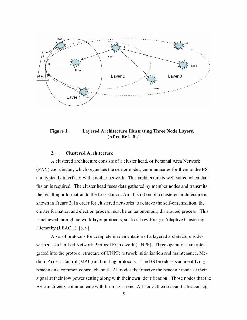
1. Layered Architecture In a layered architecture, a network consists of a base station (BS) with multiple

node layers. Grouping nodes with identical hop count to the base station forms a node

layer. An illustration of layered sensor network architecture is shown in Figure 1. The

base station acts as an access point or gateway to the wired network. The base station

gathers and disseminates data. The nodes of each layer form a wireless backbone to es-

tablish connectivity. The network participants could access the network using handheld

transceivers. These transceivers are distinguished by their human interface and would be

similar to Personal Digital Assistants (PDAs). This type of transceiver would connect to

the wireless backbone formed by the layered nodes. The architectural advantage allows

each node short communication distances and the ability to employ low transmission

power. [8]

5

Figure 1. Layered Architecture Illustrating Three Node Layers. (After Ref. [8].)

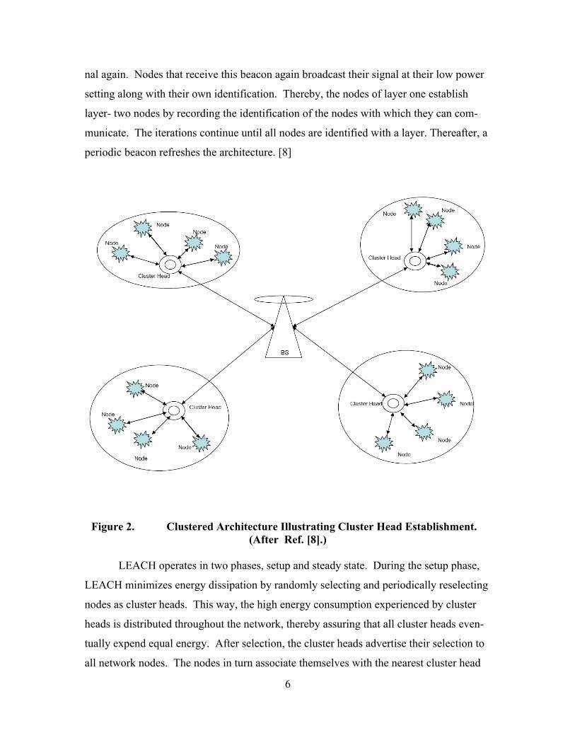
2. Clustered Architecture A clustered architecture consists of a cluster head, or Personal Area Network

(PAN) coordinator, which organizes the sensor nodes, communicates for them to the BS

and typically interfaces with another network. This architecture is well suited when data

fusion is required. The cluster head fuses data gathered by member nodes and transmits

the resulting information to the base station. An illustration of a clustered architecture is

shown in Figure 2. In order for clustered networks to achieve the self-organization, the

cluster formation and election process must be an autonomous, distributed process. This

is achieved through network layer protocols, such as Low-Energy Adaptive Clustering

Hierarchy (LEACH). [8, 9]

A set of protocols for complete implementation of a layered architecture is de-

scribed as a Unified Network Protocol Framework (UNPF). Three operations are inte-

grated into the protocol structure of UNPF: network initialization and maintenance, Me-

dium Access Control (MAC) and routing protocols. The BS broadcasts an identifying

beacon on a common control channel. All nodes that receive the beacon broadcast their

signal at their low power setting along with their own identification. Those nodes that the

BS can directly communicate with form layer one. All nodes then transmit a beacon sig-

6

nal again. Nodes that receive this beacon again broadcast their signal at their low power

setting along with their own identification. Thereby, the nodes of layer one establish

layer- two nodes by recording the identification of the nodes with which they can com-

municate. The iterations continue until all nodes are identified with a layer. Thereafter, a

periodic beacon refreshes the architecture. [8]

Figure 2. Clustered Architecture Illustrating Cluster Head Establishment. (After Ref. [8].)

LEACH operates in two phases, setup and steady state. During the setup phase,

LEACH minimizes energy dissipation by randomly selecting and periodically reselecting

nodes as cluster heads. This way, the high energy consumption experienced by cluster

heads is distributed throughout the network, thereby assuring that all cluster heads even-

tually expend equal energy. After selection, the cluster heads advertise their selection to

all network nodes. The nodes in turn associate themselves with the nearest cluster head

7

based on the received signal strength of the selection advertisement. A TDMA schedule

is then assigned for node communication. The steady-state phase is long in comparison

to the setup phase in order to minimize the overhead of cluster formation. Data transmis-

sion takes place during the steady-state phase based on the TDMA schedule established

during setup. Energy is conserved by local processing and data aggregation at the cluster

head. [9]

This section described the two broad classifications of network architecture as

layered and clustered. A technique for establishing each classification was discussed.

This discussion was designed to assist the reader in gaining perspective into how the

characteristics of self-organization and low power operation govern design of the net-

work architecture. A discussion of protocols for a typical wireless, sensor network fol-

lows.

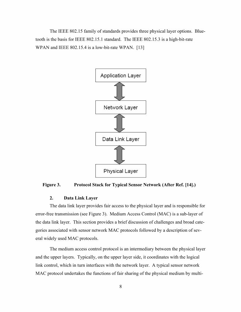
C. SENSOR NETWORK PROTOCOLS The communication functionality of a sensor network node follows layered proto-

col architecture. Figure 3 describes the typical layered protocol stack of a sensor network

node. The application layer provides mechanisms for analog-to-digital conversion. The

network layer is responsible for seamless transfer of information, and the data link layer

provides fair access and is responsible for error-free transmission. The physical layer

provides a means of sending and receiving a bit stream. In the following sections, the

functions of the different layers are discussed, and the main design issues are highlighted.

1. Physical Layer Wireless sensor networks are designed for low bit rates. The lower rate supports

the essential characteristics of longer battery life and self-organization. Wireless sensor

networks could conceivably communicate using radio or infrared techniques; the focus

here is on radio techniques. Some of the proposed radio frequency (RF) techniques are

PicoRadio, Wireless Integrated Network Sensors (WINS), and the IEEE 802.15 Stan-

dards for Wireless Personal Area Networks (WPAN). PicoRadio [10] employs ultra-

wide band at the physical layer. WINS [11] employs spread spectrum techniques in unli-

censed Industrial, Scientific, and Medical (ISM) frequency bands. [12]

8

The IEEE 802.15 family of standards provides three physical layer options. Blue-

tooth is the basis for IEEE 802.15.1 standard. The IEEE 802.15.3 is a high-bit-rate

WPAN and IEEE 802.15.4 is a low-bit-rate WPAN. [13]

Figure 3. Protocol Stack for Typical Sensor Network (After Ref. [14].)

2. Data Link Layer The data link layer provides fair access to the physical layer and is responsible for

error-free transmission (see Figure 3). Medium Access Control (MAC) is a sub-layer of

the data link layer. This section provides a brief discussion of challenges and broad cate-

gories associated with sensor network MAC protocols followed by a description of sev-

eral widely used MAC protocols.

The medium access control protocol is an intermediary between the physical layer

and the upper layers. Typically, on the upper layer side, it coordinates with the logical

link control, which in turn interfaces with the network layer. A typical sensor network

MAC protocol undertakes the functions of fair sharing of the physical medium by multi-

9

ple users and efficient utilization of the data rate. The MAC protocol supports the physi-

cal layer by optimizing the data frame size and frequency of transmission. The MAC

protocol provides energy management, flow and error control, timing and synchroniza-

tion.

Sensor network MAC protocols may be categorized into three types: fixed alloca-

tion, demand-based, and contention based. Fixed-allocation protocols share the channel

through a predetermined assignment. They are appropriate for networks that continu-

ously observe and propagate deterministic data traffic. Fixed-allocation protocols lead to

inefficiencies when the channel requirements of each node are time-varying. A time-

varying channel requires demand-based protocols, which allocate channel space based on

node demand. Although additional overhead is required to reserve the channel, they are

well suited for variable rate traffic. In contention-based protocols, nodes compete for

channel access. If the channel is busy, each node waits a random amount of time before

attempting to access the channel again. Contention-based protocols are suitable for sen-

sor networks that generate non-deterministic traffic. Time sensitive traffic may experi-

ence delay and traffic collisions are an issue. [8]

Some of the popular sensor network MAC protocols in these categories are: Self

Organizing MAC for Sensor Networks (SMACS), Eavesdrop and Register (EAR), Hy-

brid TDMA/FDMA, and CSMA-Based.

SMACS and EAR work together to handle network initialization and mobility.

SMACS is a distributed protocol for network establishment and link layer association.

SMACS handles discovery of neighbor nodes and channel assignment concurrently. The

EAR protocol provides integrated linking of nodes under moving and motionless condi-

tions. The protocol utilizes certain mobile nodes working together with static nodes to

provide connections. Mobile nodes listen for control signals to update its list of

neighbors. The mobile nodes dominate connections and terminate links degraded by mo-

bility. EAR independently handles mobility, an aspect transparent to SMACS. [15]

The hybrid TDMA/FDMA scheme is centrally regulated and assumes that nodes

converse straight to a nearby base station. A TDMA scheme minimizes delay at the cost

of time synchronization. An FDMA scheme provides the minimum bandwidth required

10

for each ling. The hybrid scheme uses an ideal number of channels to diminish overall

power expended and depends on the proportion of transmitter to receiver power expendi-

ture. If the transmitter expends greater power, a TDMA scheme is desired since it can be

turned off during idle time slots. When the receiver consumes greater power, the scheme

favors FDMA. [16]

For point-to-point, random traffic flow, traditional CSMA-based MAC schemes

are better suited. These protocols adapt well to the variable, but periodic and correlated

traffic of sensor networks. CSMA-based MAC protocols are contention-based and are

designed mainly to increase energy efficiency and maintain fair access. Woo and Culler

[16] describe a CSMA-based MAC protocol for sensor networks. Energy efficiency is

achieved by constant sensing periods. Collisions are avoided and binary exponential

back-off introduces random delay in order to avoid repeated collisions caused by the syn-

chronized nature of networked sensors. The MAC protocol also controls the rate of data

originating at the node so that nodes closer to the BS do not dominate traffic flow. [8, 17]

This section presented a description of the design challenges and types of MAC

protocols. Several widely studied protocols were briefly discussed.

3. Network Layer The network layer controls network operations. It has the traditional function of

routing packets. The distributed nature of sensor networks makes routing a challenge,

which is compounded by the low power operation of network nodes.

Routing protocols determine how data flow through the network from source to

destination. A number of routing techniques including flooding, gossiping and rumor

routing are briefly described below.

a. Routing Techniques for Layered Architecture Routing techniques for layered architecture include flooding, gossiping,

and rumor routing. “Flooding” is one routing technique in which rebroadcast occurs until

maximum destination node is reached or a maximum hop count is achieved. While the

technique avoids complexity, it does not account for duplication of received packets,

overlap of sensor coverage or available node energy. A modified version is “gossiping”

in which a packet is not broadcast but rather transmitted to a randomly chosen neighbor.

11

This avoids the problem of duplication but does not offer reliability. “Rumor” routing

uses an agent to circulate through the network recording the shortest path to events en-

countered. [8]

b. Routing Techniques for Clustered Architecture The above techniques are predominant in layered architecture networks,

which employ a base station. When the sensor nodes themselves are the destination

(peer-to-peer), rather than all queries arising from the BS, directed diffusion is a useful

protocol. The “directed diffusion” routing protocol employs interest gradients in which

the destination specifies the data-rate requirement, raising or lowering the data rate based

on the sensors’ ability to report on the destination’s interest. [19]

When a sensor network is peer enabled routing approaches include Sensor

Protocols for Information via Negotiation (SPIN), Cost-Field approach, and Geographic

Hash Table (GHT). “SPIN” overcomes the weaknesses of flooding through negotiation

and resource versatility. Negotiation reduces duplication and overlap prolonging network

lifetime. The “Cost-Field” approach uses cost as the minimum cost from the node to the

destination – the cost of the optimal path. Packets contain a cost-so-far field. Each in-

termediate node updates the cost-so-far field and continues to execute the algorithm. The

“Geographical Hash Table” (GHT) compiles keys into geographic coordinates and main-

tains the key and value at the sensor node nearest the hash value. The consistency of

mapping assures data is routed correctly. The data is distributed among nodes in a scal-

able and balanced method. [20–22]

Because of power constraints, routing protocols designed for sensor net-

works are not isolated at the network layer. The protocols gaining widest acceptance

consider efficiencies at each layer of the protocol stack shown in Figure 3. LEACH [9] is

one such protocol.

Another protocol whose design considers energy efficiency techniques

within each of the layers is XMesh. The “XMesh” protocol evolved from the initial

Surge-Reliable and Mint Route protocols developed by Hill and Woo [23]. XMesh fea-

tures include self-organizing, self-healing, low-power listening and time synchronization.

It can provide quality of service through link-level acknowledgements and end-to-end

12

acknowledgements. This protocol is capable of bulk transfer along a dedicated path,

similar to a streaming service. The algorithm awakens the node up to eight times per sec-

ond to assess the radio channel. Once awakened, the node determines if a preamble is

being transmitted. When a preamble is detected, the node prepares to receive data. If the

channel is clear, the node may transmit its own data, or retransmit data from another

node. The algorithm achieves streaming like quality via messaging to establish a network

route and dynamic voltage scaling; an increase in node transmission power to minimize

number of hops. [23–24]

The routing techniques of flooding, gossiping and rumor routing were in-

troduced followed by a description of more sophisticated techniques, such as SPIN, GHT,

SMCEN and XMesh. This was to facilitate an understanding of the adaptation used when

the sensor nodes themselves are the destination, and a directed diffusion routing protocol

is employed.

4. Application Layer Sensors form the application layer and convert physical phenomenon into trans-

mittable data. A sensor measures a physical quantity and converts this quantity into a

physical pulse, which in turn is converted into a binary code and formatted into a data

packet. The sensor information in the data packet is transmitted to a designated node, or

a base station, depending on the sensor network topology.

D. OTHER NETWORK CHALLENGES As sensor networks continue to evolve, explorations into localization, security,

energy efficiency, synchronization, and real-time communication remain. Localization is

the ability of a node to determine its physical location. The broadcast nature of sensor

networks makes them vulnerable to a variety of attacks requiring security techniques as a

deterrent. Energy efficiency requires the knowledge necessary to skillfully integrate

hardware and software techniques. Node synchronization is important in order to support

localization techniques. Real time communications are required in network surveillance

applications. [8]

13

1. Localization Location can be specified globally by the use of Global Positioning System (GPS)

satellites, or it can be specified locally by relative position from other devices in the net-

work. This section describes methods to achieve localization through signal processing

with an onboard micro-controller rather than GPS. This allows flexibility in number of

nodes and sensor composition. To effectively aggregate sensor data, node location

should be coupled with sensor information in the message transmitted by each node. A

low-power, inexpensive, accurate mechanism is desired. Utilizing a GPS receiver not

only adds bulk to the sensor board, but it also consumes high power and does not pene-

trate dense foliage or buildings. [8]

Indoor localization techniques employ strategically placed fixed beacon nodes.

These randomly distributed nodes receive beacon signals and calculate the signal

strength, angle of arrival and time difference-of-arrival from different beacon transmit-

ters. Using these measurements, the nodes estimate their position by triangulation or a

priori knowledge of beacon node locations. [25]

In outdoor situations, or when no fixed infrastructure is available and prior meas-

urements are not practical, some of the nodes themselves act as beacons. In this case, the

network requires GPS-enabled nodes to transmit beacon signals. In the case of RF com-

munications, the received signal strength indicator is a method of estimating distance de-

spite its sensitivity to obstacles and environmental conditions. Time difference-of-arrival

algorithms can improve accuracy. These localization algorithms estimate location based

on a beacon node’s location. A direction based localization approach described in [26]

assumes that the beacon nodes broadcast to all nodes in the network and that a central

controller pivots the beacons at a continuous angular velocity. [8, 25–26]

2. Security

The characteristics of wireless sensor networks constrain established techniques

for security. Effective security measures require a means of assuring data authentication,

data integrity and maintain privacy. Data authentication requires an asymmetric mecha-

nism to avoid message forgery. Data integrity assures that the received data are not al-

tered. [7–8, 20]

14

Sensor nodes depend on repetitive forwarding by broadcast for message propaga-

tion through the network. Selective forwarding attacks are intentional and occur when a

node fails to forward packets. A “sinkhole attack” is a form of selective forwarding and

occurs where a node falsely advertises the most efficient route. Once the malicious node

receives multi-hopped traffic, it begins selective forwarding. Sensor networks are vul-

nerable to this type of attack because most information is transmitted toward the BS. [8]

The importance of security among networked sensors stems from the significant

trust level assumed during data aggregation and event detection. Symmetric or public-

key cryptography’s high processing requirements make them unsuitable for many low-

power sensor network deployments. If the processing power is supportable, Localized

Encryption and Authentication Protocol (LEAP) and Intrusion Tolerant Routing in Wire-

less Sensor Networks (INSENS) may be employed. [8, 28–31]

Security Protocols for Sensor Networks (SPINS) consist of a number of ideal pro-

tocols for extremely resource-constrained sensor networks. SPINS consist of two pri-

mary components a sensor network encryption protocol (SNEP) and a micro-version of

the timed, efficient, streaming loss-tolerant authentication protocol ( TESLA).µ SNEP

provides data authentication, protection from replay attacks and semantic security at a

cost of only eight bytes per message. Semantic security prevents an adversary from de-

termining the plaintext message even after observing multiple encrypted versions of the

same plain text by employing a shared counter and incrementing the counter after each

block. A replay attack is the introduction of an old alarm message as a current message

and is prevented by a counter value carried by the message. Data authentication is veri-

fied at the MAC layer. Message integrity and authentication are provided through use of

a message authentication code – similar to a checksum derived by applying a secret

shared key to the message. [20]

The protocol TESLAµ ensures that a broadcast is authenticated, thereby assuring

the receiver of the sender’s identity. The protocol allows imprecise time synchronization

to exist between the nodes. The BS and each node share knowledge on the maximum

synchronization error’s upper bound. Asymmetric cryptographic keys have high over-

15

head. The protocol TESLAµ overcomes this problem by delaying the disclosure of sym-

metric keys to achieve asymmetry, which provides data authentication. [20]

3. Energy Management

The stringent energy constraint of sensor nodes requires optimization to prolong

single node and network lifetime. A node’s measure of efficiency is the ratio of data de-

livered to energy expended. Efficient energy management must be designed into both

hardware and software.

Energy efficiency techniques must look to optimize network and node lifetime.

The optimization of the hardware level requires employing dynamic power management

to each device. Dynamic power management is a technique to shut down node compo-

nents when no events take place. Dynamic voltage scaling (DVS) is another technique

for hardware optimization. Dynamic voltage scaling accounts for the processor’s time

varying computational load – the voltage is scaled to meet only the instantaneous proces-

sor requirements. The operating system, application and network software, should be

designed with energy awareness. Voltage is not the only determinant of network life-

time. Considerable energy is consumed by the sleep current of network devices and by

the method of routing. [8, 32]

4. Synchronization Synchronization requires all nodes to agree on time. Synchronization must con-

form to the low power characteristics of wireless sensor networks to preserve network

lifetime.

Node synchronization is required to sustain TDMA schemes on wireless-mesh

networks. Synchronization is also necessary to organize messages by time sent from the

sensors. Synchronization allows nodes the capability to determine their relative position

when deployed randomly. To achieve data aggregation, the sensor must be able to pre-

cisely determine the instant in time at which an event occurred in order to recognize du-

plication. [8]

There are two major categories of synchronization algorithms. The first category

achieves long-lasting global synchronization. The second category achieves short-lived,

or pulsed synchronization, where nodes are synchronized only for an instant. A low

16

power synchronization scheme proposed by [33] performs local synchronization by

means of a broadcast beacon, from which all nodes normalize their time stamps for ob-

servation of the event. This scheme creates short-lived synchronization for nodes within

transmission range of the beacon. [8, 33]

A global synchronization protocol described in [34] is based on knowledge of the

neighboring nodes control signal. A node leader is elected by majority vote. The leader

periodically transmits synchronization messages to its neighbors. These messages are

rebroadcast to all networked nodes.

Resynchronization is required in dynamic networks where topology and mobility

require synchronization of node clusters to a universal clock. Resynchronization is re-

quired in situations such as the merging of two clusters due to mobility. In this case, the

clocks of each cluster need to be updated to match the clock of the node chosen as net-

work coordinator. [8, 33]

5. Real-Time Communication Sensor networks should support real-time communications. The time between

sensing an event and communicating the event is a measure of network quality. Real-

time communications implies minimal delay experienced in reporting events. The event

must efficiently propagate toward the cluster-head or base station. Two protocols that

support real-time communication are SPEED and RAP.

The SPEED protocol supports real-time communication in sensor networks by

guaranteeing maximum delay. RAP allows applications to concentrate their queries to

nodes or portions of the network. The BS or cluster head contains an application layer

program that specifies the event information desired, the area to which the query is ad-

dressed, and the information reporting deadline. The underlying layers of RAP ensure

the communication of the query to all nodes specified in the address and communication

of the query results to the BS. [35–36]

E. SENSOR CHARACTERISTICS Having explored the characteristics of wireless sensor networks and their impact

on network architecture and protocols, attention is now turned toward the sensor tech-

17

nologies. This section describes sensor operation and introduces characteristics of an

ideal sensor. The principles governing the operation of an ideal sensor provide a frame-

work for discussion of temperature/humidity, acoustic, magnetic, position, acceleration,

light, barometric, and infrared sensors.

Low power, high fidelity and small form factor are desirable features of a sensor.

The ideal sensor for networks would therefore have zero mass, zero volume, and infinite

bandwidth and require zero signal energy. The zero mass and volume would enhance

acceleration and pressure sensors. Infinite bandwidth would improve any sensor, but

most useful for video sensors and zero energy requirements remains an unproven ideal.

These idealized notions have led research efforts into miniature micro electro-mechanical

devices. [37–38]

While not theoretically ideal, modern sensor technologies are relatively small and

low power. However, there is a price for miniaturization. As form factor constraints re-

duce sensor size, operating power densities increase proportionally, resulting in decreased

static stability. The decrease in static stability claim is based on comparison with larger

and more massive sensor designs. This decrease in stability is a design factor in minia-

turization but not a deterrent to miniaturization. [37–38]

Another factor influencing sensor miniaturization is the Heisenberg uncertainty

principle, which assures that every sensor is influenced by more than its measured phe-

nomenon. For example, the intent may have been to measure pressure, but the measure-

ment of pressure reflects all aspects of the physical world, such as temperature and hu-

midity. By understanding these interactions, sensor designers are able to improve the

quality of measurement. [37–38]

The characteristics of an ideal sensor provide a framework for discussion and de-

scription of several specific types of sensors.

1. Temperature/Humidity Sensors

Temperature can be measured by several types of instruments; thermocouples are

the most common technique for sensor networks. A thermocouple is a junction of dis-

similar metals, which produces a small electromotive force due to the temperature differ-

ences. [37]

18

Relative humidity is the ratio of the actual vapor pressure of the air at any tem-

perature to the maximum of saturation vapor pressure at the same temperature. Relative

humidity H represents vapor content as a percentage of the concentration required to

cause the vapor to saturate, i.e., the formation of water droplets (dew) at that temperature.

In percent, H is defined as:

100w

s

PHP

= × (2.1)

where wP the partial pressure of water vapor and sP is the pressure of saturated water va-

por at a given temperature. [37]

Relative humidity and temperature can be obtained using Sensirion’s SHT11 sen-

sor, which allows for relative humidity readings from 0 to 100% with an accuracy of

3%± using an optical hygrometer. The basic idea of an optical hygrometer is the use of

a mirror whose temperature is precisely controlled at the threshold for dew formation.

Air is sampled and pumped across the mirror’s surface. If the mirror temperature crosses

a dew point, it releases moisture in the form of water droplets. The water droplets scatter

light rays projected onto the mirror surface. This scattering is detected by a photodetec-

tor. The relative humidity can be obtained from the dew point and the prevailing tem-

perature. The temperature is measured by means of a thermocouple; accuracy is 5±

at 25 C , and the power consumption is rated at 30 Wµ . [23–39]

2. Acoustic Sensor

Acoustic sensors rely upon alternate expansion and compression of sound waves.

Whenever sound is produced, air is alternately compressed and rarefied, and these pres-

sure differences propagate outward as sound waves. A general equation for pressure ex-

erted by a sound wave is

( )sinmp p kx tω= − (2.2)

where mp is the magnitude of the sound pressure, 2k π λ= is a wave number (λ is

wavelength), and ω is angular frequency. [37]

19

Pressure levels, ,Π can also be expressed in decibels as

10

0

[dB] 20log pp

=

∏ (2.3)

where28 9

0 2 10 N/m 2 10 psip −= × = × . This pressure subjects a crystalline piezoelectric

material to stress and generates an electric charge proportional to input pressure. [37]

In the National Semiconductor LMC567 Low Power Tone Decoder, the piezo-

electric charge produced by the pressure levels of Equation 2.3 provides input to a Volt-

age-Controlled Oscillator (VCO). The VCO establishes reference signals for phase and

amplitude detection. The phase and amplitude detectors are devices that produce a meas-

ure of the difference in phase and amplitude, respectively, between an incoming signal

and the output of the VCO. As the incoming signal and the output of the VCO change

with respect to each other, the difference becomes the time-varying signal. The output of

the phase detector is input to the VCO to aid in tracking the incoming signal. The output

of the amplitude detector is a measure of the received tone. The device can operate with

supply voltage varying from 2 V to 9 V and at input frequencies ranging from 1 Hz to

500 kHz. Low supply current drain is possible through tradeoffs in the resistor and ca-

pacitor values of the timing circuit. Additionally, out-of-band signals and noise are re-

jected. [40–41]

3. Magnetic Sensor One of the many advantages of using magnetic field for sensing position and dis-

tance is that the field can penetrate any nonmagnetic material with no loss of position ac-

curacy. The magneto-resistive effect is the ability of a material to change its resistivity in

the presence of a magnetic field. This is a well-established property of magnetic material

with carrying a current. This change in resistivity is created by the materials’ magnetic

field rotating relative to current direction. Most conductors’ resistivity increases in the

presence of a magnetic field. The basic cause of magnetoresitivity is the Lorentz force,

which causes electrons to move in curved paths between collisions. The Lorentz force,

,F on a moving particle when both electric and magnetic fields are present is given by

F qE qU B= + x (2.4)

20

where q is the charge, E is the electric field, U is the velocity vector of the charged par-

ticle and B is the magnetic field strength. [37–42]

Magneto-resistive sensors determine a change in earth’s magnetic field due to the

presence of a ferromagnetic object or due to change in position within earth’s magnetic

field. A magneto-resistive sensor is fabricated of permalloy strips (80/20 alloy of Ni and

Fe) positioned on an arm of a wheatstone bridge. The degree of the bridge imbalance is

then used to indicate the magnetic field strength. Honeywell HMC1002 two-axis mag-

netic sensor has a field range of 6± gauss. The two-axis sensor can work together to pro-

vide three-axis sensing. Configured as a four-element wheatstone bridge, these magneto-

resistive sensors convert magnetic fields to a differential output voltage and are capable

of sensing magnetic field as low as 30 gaussµ . (The Earth’s magnetic field is 0.5 gauss.)

The sensor reports the magneto-resistive effect in terms of mutual gauss (mgauss). High

bandwidth provides the opportunity to detect vehicles and other ferrous objects at high

speeds. The sensor’s operational range is dependent on the ferromagnetic mass meas-

ured. The NiFe permalloy core sensitivity makes it subject to saturation when the sensor

is exposed to a large magnetic field. [40, 43]

4. Position Sensor Localization is a technique for sensing position where the reliance is on signal

processing at the node level. Localization techniques in outdoor scenarios still require a

portion of the network to be GPS enabled. GPS is the predominant form of position

sensing. The simple GPS receiver stores the pseudo-random code of each of the GPS

satellites in memory. By identifying the code, the receiver knows which satellite is send-

ing each signal. Comparing the delay between the receiver’s pseudo-random code and

that generated by the satellite determines travel time. Multiplying travel time by the

speed of light determines distance. By recording these measurements for several satel-

lites, position can be determined by triangulation. GPS satellites employ an atomic clock

and predictable orbits to reduce the error. Error information is transmitted along with

timing signals. The position is determined from multiple range measurements and com-

puted by the receiver in earth-centered X, Y, Z coordinates and then converted to latitude,

longitude and height. [44]

21

The small-form factor of the Leadtek GPS 9546 makes them well suited for sen-

sor networks. This GPS provides twelve channels for in-view tracking. It is designed

with a Cold/Warm/Hot start time of 45/38/8 seconds with reacquisition in 0.1 seconds.

Its accuracy rating is within ten meters when determining latitude and longitude. It is

rated to withstand high velocity, acceleration up to 4 g, and altitudes up to 18 kilometers,

and its trickle power duty cycle is designed to reduce power consumption to 65 mW. [40,

45]

5. Acceleration Sensor The accelerometer is the primary form of motion sensing (static acceleration). It

is designed to measure the rate of change of position, location or displacement of an ob-

ject. Vibration is dynamic acceleration and a mechanical phenomenon that involves peri-

odic motion around a reference position.

A mathematical model of an accelerometer is represented by

0

( ) ( ) ( )t

x t g t a dτ τ τ= −∫ (2.5)

where x is the instantaneous acceleration at time t, a is the time-dependent impulse of the

accelerometer and ( )g t is time-dependent, a delayed version of a. The equation can be

solved for different acceleration inputs applied. The correctly designed accelerometer

possesses a clearly identifiable resonant frequency and a flat frequency response at which

the most accurate measurement can be made. [37]

By measuring the acceleration, it is easy to determine both the speed and position

of the object as well. The Analog Devices ADXL202E Dual Axis Accelerometer pro-

vides two-axis acceleration measurements on a single integrated chip. Its form factor is

5 mm 5 mm 2 mm × × and consumes less than 0.6 mA. It will measure accelerations

with a full-scale range of 2 g± and has a 1000-g shock survival. The device can measure

both dynamic acceleration (vibration) and static acceleration (gravity). The outputs are

analog voltages or digital signals whose duty cycle (pulse width/period) is proportional to

acceleration, and the device resolution is 2 g at 60 Hz. [40], [46]

22

6. Light Sensor

The process of optical detection involves the direct conversion of optical energy

(photons) into an electrical signal (moving electrons). One technique for optical detec-

tion is to employ a photodiode. [37]

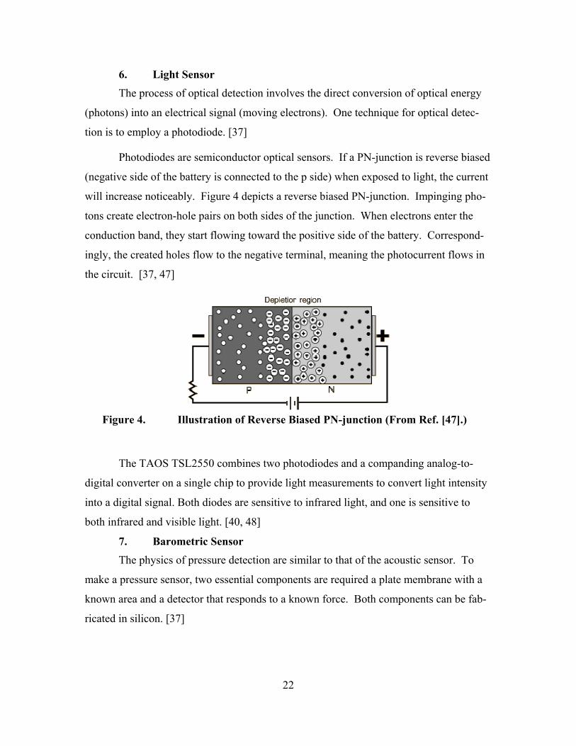
Photodiodes are semiconductor optical sensors. If a PN-junction is reverse biased

(negative side of the battery is connected to the p side) when exposed to light, the current

will increase noticeably. Figure 4 depicts a reverse biased PN-junction. Impinging pho-

tons create electron-hole pairs on both sides of the junction. When electrons enter the

conduction band, they start flowing toward the positive side of the battery. Correspond-

ingly, the created holes flow to the negative terminal, meaning the photocurrent flows in

the circuit. [37, 47]

Figure 4. Illustration of Reverse Biased PN-junction (From Ref. [47].)

The TAOS TSL2550 combines two photodiodes and a companding analog-to-

digital converter on a single chip to provide light measurements to convert light intensity

into a digital signal. Both diodes are sensitive to infrared light, and one is sensitive to

both infrared and visible light. [40, 48]

7. Barometric Sensor The physics of pressure detection are similar to that of the acoustic sensor. To

make a pressure sensor, two essential components are required a plate membrane with a

known area and a detector that responds to a known force. Both components can be fab-

ricated in silicon. [37]

23

A silicon-diaphragm pressure sensor consists of a thin silicon diaphragm as an

elastic material and piezoresistive gauge resistors. Because of the properties of single-

crystal silicon, the membrane displays elasticity with increased sensitivity, reduced error,

and no hysteresis. The MS5534B barometric sensor from Intesema contains a piezoresis-

tive pressure sensor and an ADC-interface. It provides a 16-bit data word from a pres-

sure- and temperature- dependent voltage. The module contains six readable coefficients

for calibration accuracy. The device is designed for low power, operates from a supply

voltage of 2.2 V to 3.6 V, and is configured for automatic on/off switching. The pressure

range is form 0-1100 mbar and the system clock operates at 32.768 kHz. [37, 40, 49]

8. Passive Infrared (PIR) Sensor A PIR sensing element must be responsive to infrared radiation within a spectral

range where most of the power emanated by humans is concentrated (4 to 20 mµ ).

There are three types of potentially useful sensing elements: thermistors, thermopiles and

pyroelectrics. Pyroelectrics are exclusively used in motion detection applications be-

cause of they are simple, inexpensive and responsive across a broad dynamic range. [37]

A pyroelectric material generates an electric charge in response to thermal energy

flow through its body. The absorbed heat causes the front side of the sensing element to

expand. The resulting thermal expansion induces a voltage. Charge can also be induced

when subject to an external force, which is often indistinguishable from those produced

by thermal energy. Thermally induced charges are separated from external force-induced

charges by manufacturing pyroelectric sensors in a symmetrical form. Two elements are

connected to the electronic circuit to produce out-of-phase signals when subjected to the

same input. [37]

A typical infrared non-contact sensor consists of a sensing element, protective

window, support structure, housing and connectors. The sensing element is a component

that is sensitive to electromagnetic radiation in the infrared wavelength. The protective

window is impermeable to environmental factors and transparent to the wavelength of

detection. The operating principle is based on the sequential conversion of thermal radia-

tion into heat, followed by conversion of heat level into an electrical signal. Infrared

24

sensors produced by Omega offer six infrared spectral responses. They are sensitive

across a temperature range of 50°F to 200°F with adjustable response time from 0.2 to

5.0 s. [37, 40, 50]

In this chapter, the characteristics of wireless sensor network were described fol-

lowed by a detailed description of layered and clustered architectures. The protocol stack

for a typical sensor network and the associated functions were discussed. The challenges

associated with localization, security, energy management, synchronization, and real-time

communication were described. The characteristics of an ideal sensor were introduced

followed by a description of several types of sensors. A discussion of the IEEE 802.15

family of standards and the details of the network prototyped in this thesis follows in the

next chapter.

25

III. NETWORK PROTOTYPE

In designing wireless sensor networks, several of their unique requirements need

to be taken into account. Selection of the sensor, or sensors, that meet the application-

specific need is the first of them. The radio frequency band in which the network is re-

quired to operate and the range of coverage are determined by the terrain and electro-

magnetic conditions and, therefore, must also be considered. The reader may note that

these requirements are in addition to the requirements, such as energy and size, indicated

in the previous chapter.

This chapter provides a summary of the IEEE 802.15 family of standards fol-

lowed by a description of the IEEE 802.15.4 standard. A discussion of network hardware

and software is included. The details of the prototyped network are described.

A. IEEE 802.15.4 STANDARD FOR LOW RATE PERSONAL AREA NETWORKS

A number of wireless network standards, such as the IEEE 802.11, are available,

which in principle can be used for gathering and dissemination of sensor data. Neverthe-

less, the IEEE 802.15.4 is a standard specifically developed for low-rate sensor networks.

This section provides an overview of the various standards designed for wireless personal

area networks (WPANs). The current standards in the IEEE 802.15 family are IEEE

802.15.1, IEEE 802.15.3, and IEEE 802.15.4. A discussion of these standards provides a

basis for establishing a preferred standard.

IEEE Standard 802.15.1 (Bluetooth) was the first Wireless Personal Area Net-

work (WPAN) standard to be licensed. Its architecture is based upon the slave – master

concept and forming of piconets. The modulation technique used is frequency hopping

spread spectrum, and the clock of the master synchronizes all slaves to the frequency

hopping channel. When multiple piconets overlap, they form a “scatternet”; a Bluetooth

device can participate in several piconets at the same time. Channel access is governed

by a time division duplexing scheme. [13]

26

The IEEE Standard 802.15.3 supports ad hoc connections, quality of service

(QoS), and high speed (up to 55 Mbits per second). The network architecture employs

piconets. Piconet Coordinators (PNC) maintain synchronization, supervise QoS and

power save modes, and manages authentication. The physical layer operates at 2.4 GHz,

and the standard supports six distinct modulation techniques. The MAC layer utilizes

CSMA and TDMA to allow the transportation of synchronous and asynchronous data. A

beacon sent at the beginning of each frame is used to synchronize the PNC and the net-

work nodes. [13]

The IEEE 802.15.4 standard was developed to support networks of ultra low

power at low cost. The network is composed of full function and reduced function nodes.

The physical layer operates at 2.4-GHz and 915-MHz bands in the United States. The

915-MHz band operates over ten channels and uses binary phase shift keying modulation.

The 2.4-GHz band operates over sixteen channels and uses offset quadrature phase shift

keying modulation. The MAC layer uses CSMA/CA for channel access. [51] A de-

tailed description of this standard is provided below.

Many applications require short range wireless connectivity, ultra-low power con-

sumption and low cost. Sensor networks contain thousands of interconnected sensors

with a desired battery life of up to several years. With battery life as a key criterion, net-

work designers traded high data rate for long battery life. The IEEE 802.15.1 and IEEE

802.15.3 standards support high data rates but do not offer low power and low cost. Sen-

sor networks are an application of the IEEE 802.15.4 standard. Low-power consumption

is a unique requirement of wireless sensor networks. The ability to self-organize and es-

tablish reliable communication at low cost are desired characteristics. The network for-

mation, the physical layer and the MAC layer are described in the following section. [13,

51]

1. Network Formation

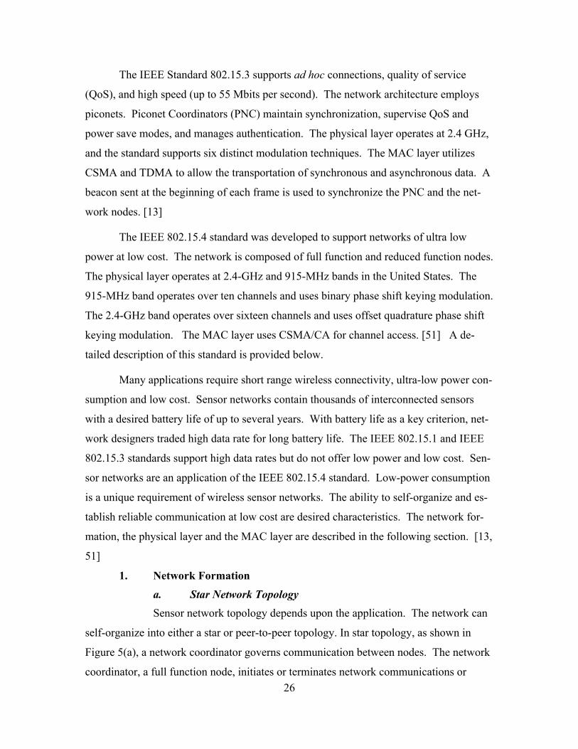
a. Star Network Topology

Sensor network topology depends upon the application. The network can

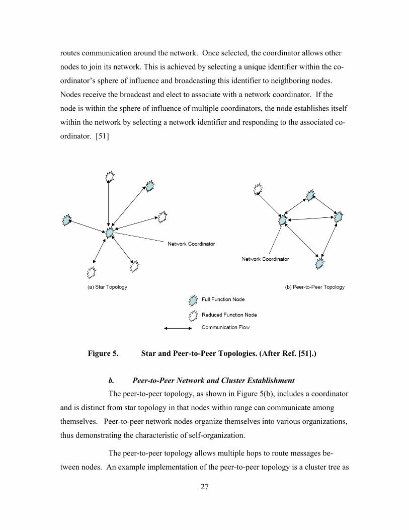
self-organize into either a star or peer-to-peer topology. In star topology, as shown in

Figure 5(a), a network coordinator governs communication between nodes. The network

coordinator, a full function node, initiates or terminates network communications or

27

routes communication around the network. Once selected, the coordinator allows other

nodes to join its network. This is achieved by selecting a unique identifier within the co-

ordinator’s sphere of influence and broadcasting this identifier to neighboring nodes.

Nodes receive the broadcast and elect to associate with a network coordinator. If the

node is within the sphere of influence of multiple coordinators, the node establishes itself

within the network by selecting a network identifier and responding to the associated co-

ordinator. [51]

Figure 5. Star and Peer-to-Peer Topologies. (After Ref. [51].)

b. Peer-to-Peer Network and Cluster Establishment

The peer-to-peer topology, as shown in Figure 5(b), includes a coordinator

and is distinct from star topology in that nodes within range can communicate among

themselves. Peer-to-peer network nodes organize themselves into various organizations,

thus demonstrating the characteristic of self-organization.

The peer-to-peer topology allows multiple hops to route messages be-

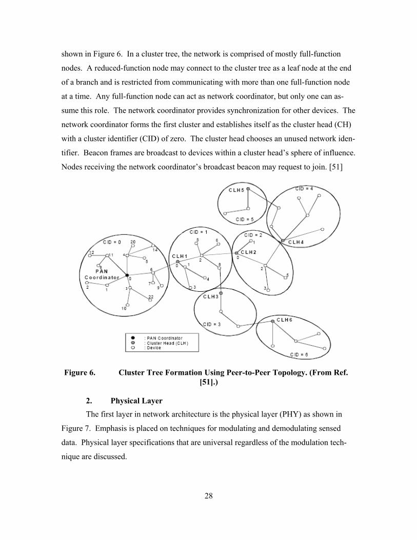
tween nodes. An example implementation of the peer-to-peer topology is a cluster tree as

28

shown in Figure 6. In a cluster tree, the network is comprised of mostly full-function

nodes. A reduced-function node may connect to the cluster tree as a leaf node at the end

of a branch and is restricted from communicating with more than one full-function node

at a time. Any full-function node can act as network coordinator, but only one can as-

sume this role. The network coordinator provides synchronization for other devices. The

network coordinator forms the first cluster and establishes itself as the cluster head (CH)

with a cluster identifier (CID) of zero. The cluster head chooses an unused network iden-

tifier. Beacon frames are broadcast to devices within a cluster head’s sphere of influence.

Nodes receiving the network coordinator’s broadcast beacon may request to join. [51]

Figure 6. Cluster Tree Formation Using Peer-to-Peer Topology. (From Ref. [51].)

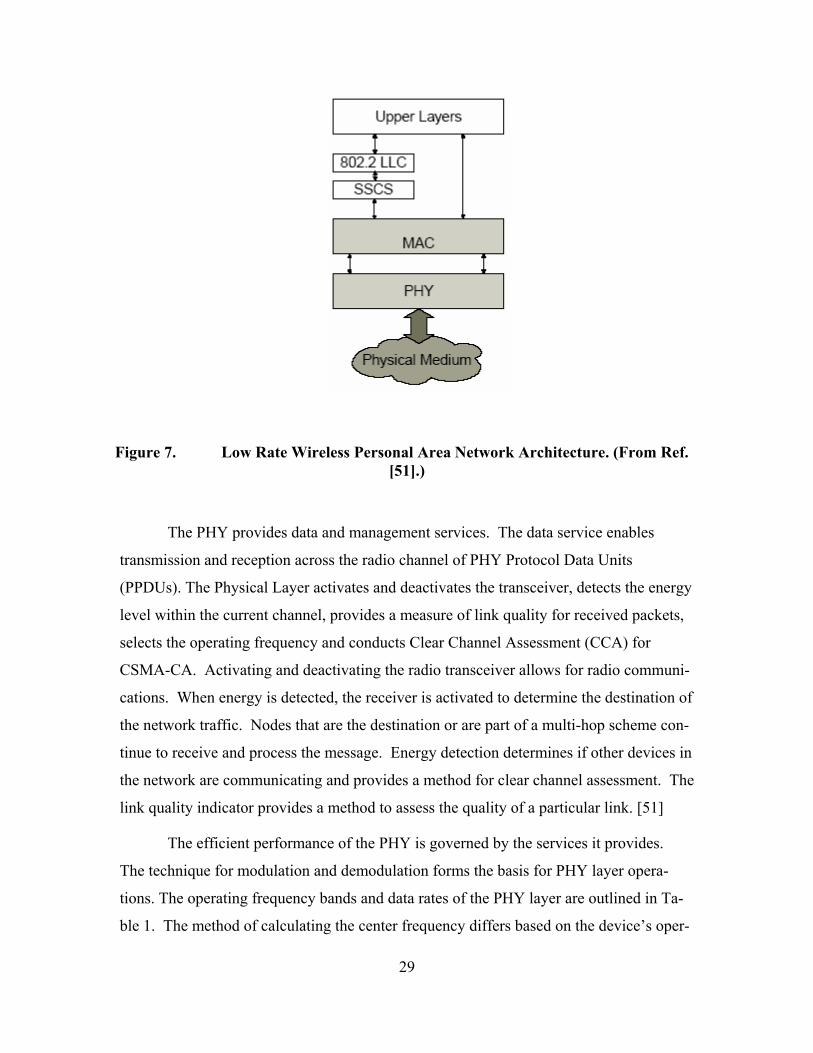
2. Physical Layer

The first layer in network architecture is the physical layer (PHY) as shown in

Figure 7. Emphasis is placed on techniques for modulating and demodulating sensed

data. Physical layer specifications that are universal regardless of the modulation tech-

nique are discussed.

29

Figure 7. Low Rate Wireless Personal Area Network Architecture. (From Ref. [51].)

The PHY provides data and management services. The data service enables

transmission and reception across the radio channel of PHY Protocol Data Units

(PPDUs). The Physical Layer activates and deactivates the transceiver, detects the energy

level within the current channel, provides a measure of link quality for received packets,

selects the operating frequency and conducts Clear Channel Assessment (CCA) for

CSMA-CA. Activating and deactivating the radio transceiver allows for radio communi-

cations. When energy is detected, the receiver is activated to determine the destination of

the network traffic. Nodes that are the destination or are part of a multi-hop scheme con-

tinue to receive and process the message. Energy detection determines if other devices in

the network are communicating and provides a method for clear channel assessment. The

link quality indicator provides a method to assess the quality of a particular link. [51]

The efficient performance of the PHY is governed by the services it provides.

The technique for modulation and demodulation forms the basis for PHY layer opera-

tions. The operating frequency bands and data rates of the PHY layer are outlined in Ta-

ble 1. The method of calculating the center frequency differs based on the device’s oper-

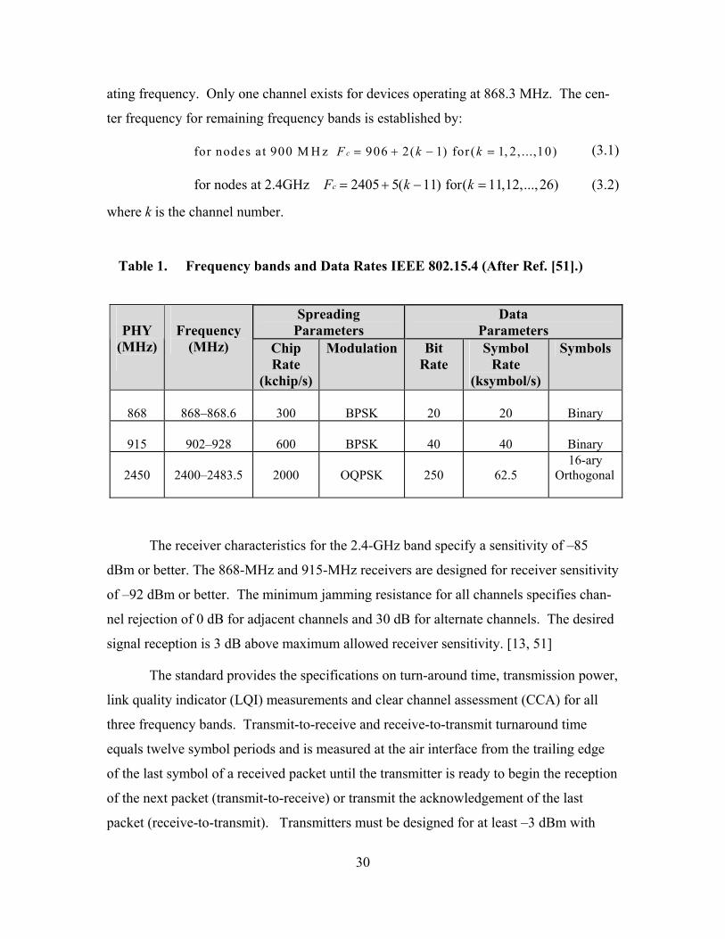
30

ating frequency. Only one channel exists for devices operating at 868.3 MHz. The cen-

ter frequency for remaining frequency bands is established by:

for nodes at 900 M H z 906 2( 1) for ( 1, 2, ...,10)cF k k= + − = (3.1)

for nodes at 2.4GHz 2405 5( 11) for( 11,12,...,26)cF k k= + − = (3.2)

where k is the channel number.

Table 1. Frequency bands and Data Rates IEEE 802.15.4 (After Ref. [51].)

The receiver characteristics for the 2.4-GHz band specify a sensitivity of –85

dBm or better. The 868-MHz and 915-MHz receivers are designed for receiver sensitivity

of –92 dBm or better. The minimum jamming resistance for all channels specifies chan-

nel rejection of 0 dB for adjacent channels and 30 dB for alternate channels. The desired

signal reception is 3 dB above maximum allowed receiver sensitivity. [13, 51]

The standard provides the specifications on turn-around time, transmission power,

link quality indicator (LQI) measurements and clear channel assessment (CCA) for all

three frequency bands. Transmit-to-receive and receive-to-transmit turnaround time

equals twelve symbol periods and is measured at the air interface from the trailing edge

of the last symbol of a received packet until the transmitter is ready to begin the reception

of the next packet (transmit-to-receive) or transmit the acknowledgement of the last

packet (receive-to-transmit). Transmitters must be designed for at least –3 dBm with

Spreading Parameters

Data Parameters

PHY

(MHz)

Frequency

(MHz) Chip Rate

(kchip/s)

Modulation Bit Rate

Symbol Rate

(ksymbol/s)

Symbols

868

868–868.6

300

BPSK

20

20

Binary

915

902–928

600

BPSK

40

40

Binary

2450

2400–2483.5

2000

OQPSK

250

62.5

16-ary Orthogonal

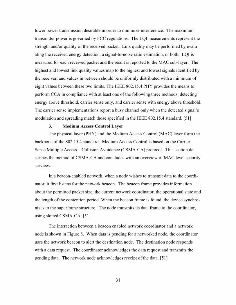
31

lower power transmission desirable in order to minimize interference. The maximum

transmitter power is governed by FCC regulations. The LQI measurements represent the

strength and/or quality of the received packet. Link quality may be performed by evalu-

ating the received energy detection, a signal-to-noise ratio estimation, or both. LQI is

measured for each received packet and the result is reported to the MAC sub-layer. The

highest and lowest link quality values map to the highest and lowest signals identified by

the receiver, and values in between should be uniformly distributed with a minimum of

eight values between these two limits. The IEEE 802.15.4 PHY provides the means to

perform CCA in compliance with at least one of the following three methods: detecting

energy above threshold, carrier sense only, and carrier sense with energy above threshold.

The carrier sense implementations report a busy channel only when the detected signal’s

modulation and spreading match those specified in the IEEE 802.15.4 standard. [51]

3. Medium Access Control Layer The physical layer (PHY) and the Medium Access Control (MAC) layer form the

backbone of the 802.15.4 standard. Medium Access Control is based on the Carrier

Sense Multiple Access – Collision Avoidance (CSMA-CA) protocol. This section de-

scribes the method of CSMA-CA and concludes with an overview of MAC level security

services.

In a beacon-enabled network, when a node wishes to transmit data to the coordi-

nator, it first listens for the network beacon. The beacon frame provides information

about the permitted packet size, the current network coordinator, the operational state and

the length of the contention period. When the beacon frame is found, the device synchro-

nizes to the superframe structure. The node transmits its data frame to the coordinator,

using slotted CSMA-CA. [51]

The interaction between a beacon enabled network coordinator and a network

node is shown in Figure 8. When data is pending for a networked node, the coordinator

uses the network beacon to alert the destination node. The destination node responds

with a data request. The coordinator acknowledges the data request and transmits the

pending data. The network node acknowledges receipt of the data. [51]

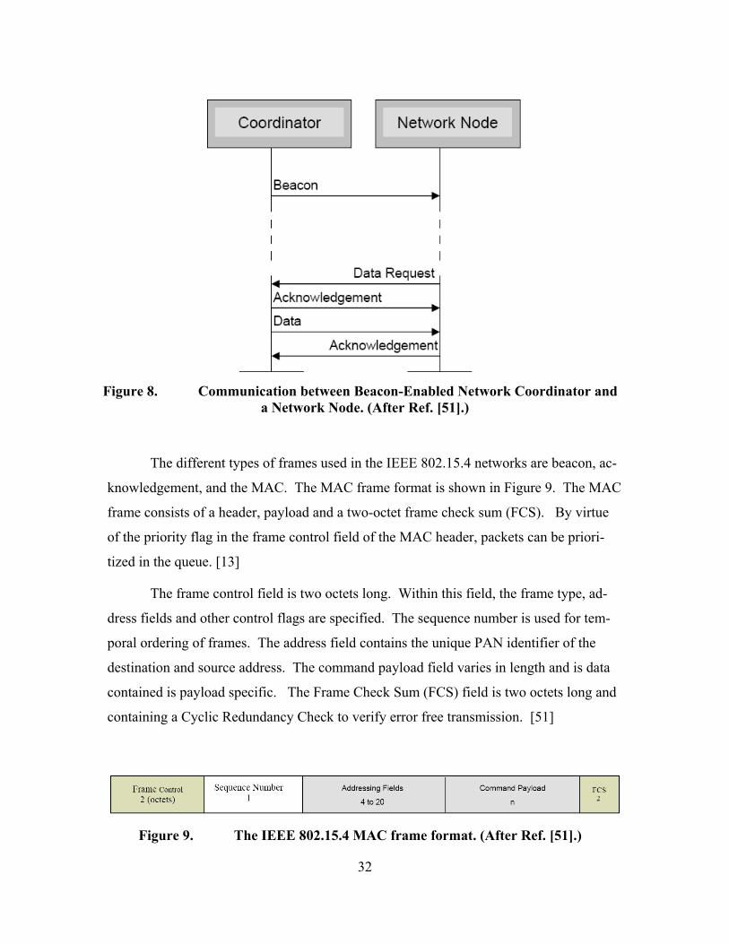
32

Figure 8. Communication between Beacon-Enabled Network Coordinator and a Network Node. (After Ref. [51].)

The different types of frames used in the IEEE 802.15.4 networks are beacon, ac-

knowledgement, and the MAC. The MAC frame format is shown in Figure 9. The MAC

frame consists of a header, payload and a two-octet frame check sum (FCS). By virtue

of the priority flag in the frame control field of the MAC header, packets can be priori-

tized in the queue. [13]

The frame control field is two octets long. Within this field, the frame type, ad-

dress fields and other control flags are specified. The sequence number is used for tem-

poral ordering of frames. The address field contains the unique PAN identifier of the

destination and source address. The command payload field varies in length and is data

contained is payload specific. The Frame Check Sum (FCS) field is two octets long and

containing a Cyclic Redundancy Check to verify error free transmission. [51]

Figure 9. The IEEE 802.15.4 MAC frame format. (After Ref. [51].)

33

In addition to medium access, the MAC layer also implements the security func-

tion. The MAC operates in two security modes, access control list (ACL) and secure.

The ACL method specifies the nodes with which communication is acceptable, and filters

all frames based on the frame’s source address. The ACL is also checked for outgoing

frames to assure an approved receiving node. The secure mode has four security ser-

vices: access control, data encryption, frame integrity and sequential freshness. Security

implementation for IEEE 802.15.4 is similar to that of IEEE 802.11. A combined sym-

metric encryption and authentication algorithm called CTR+CBC_MAC is used to pro-

vide all four security services. The operations are performed on blocks of data, thereby

lending itself well for a parallel implementation. Employment of a symmetric authentica-

tion algorithm and block cipher enables input data integrity. [13]

B. SENSOR NETWORK COMPONENTS

The PHY and MAC layer detail the inherent requirements for nodes to communi-

cate in a sensor network. The basic network components are sensors and transceivers.

This research employed the Crossbow family of sensors, transceivers and gateways. The

industry refers to the nodes as “motes”, and this terminology is adopted here. Motes are

an open source hardware and software platform combining sensing, communication and

computing into a complete architecture. The hardware design consists of a small low-

power radio and processor board known as a mote processor/radio (MPR) and a mote

sensor board (MTS), one or more sensors integrated into a single design. The MPR

board includes a processor, radio, A/D converter and battery. Many combinations exist

for creating MPR and MTS boards. When combined, the two types of boards form a sen-

sor capable of networking. To adhere to the low-power criteria, this combination typi-

cally consumes 100 mW while active and 30 Wµ in the idle mode. [40]

The connectivity and functionality of different sensor network components are

depicted in Figure 10. The PC programs the sensor either through a gateway interface as

depicted or over the air by the Deluge component in TinyOS. The application program

runs on the sensors. The sensed data are passed to the microcontroller. The microcon-

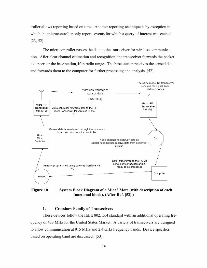
34

troller allows reporting based on time. Another reporting technique is by exception in

which the microcontroller only reports events for which a query of interest was cached.

[23, 52]

The microcontroller passes the data to the transceiver for wireless communica-

tion. After clear channel estimation and recognition, the transceiver forwards the packet

to a peer, or the base station, if in radio range. The base station receives the sensed data

and forwards them to the computer for further processing and analysis. [52]

Figure 10. System Block Diagram of a Mica2 Mote (with description of each functional block). (After Ref. [52].)

1. Crossbow Family of Transceivers

These devices follow the IEEE 802.15.4 standard with an additional operating fre-

quency of 433 MHz for the United States Market. A variety of transceivers are designed

to allow communication at 915 MHz and 2.4 GHz frequency bands. Device specifics

based on operating band are discussed. [53]

35

The 433-MHz band offers the longest range for the same output power. It has

four channels with a 500-kHz spacing. The 915-MHz frequency band operates between

902 MHz and 928 MHz. This band offers forty-eight channels with a 500-kHz band-

width and 500-kHz spacing between channels. The 2.4-GHz band is acceptable world-

wide and has a larger bandwidth. The 2.4-GHz band offers sixteen channels as defined by

the IEEE 802.15.4 standard. [23, 53]

The construction and functionality of the motes is dependent upon the frequency

band selected. Crossbow’s family of motes is recognized by trade names MICA,

MICA2, MICA2DOT and MICAz. The subcomponents of the MICA2 mote are detailed

in Table 3. All Mica motes utilize the same subcomponents with the exception of the

MICAz whose radio is slightly different. A description of the component features fol-

lows. The governing principal in mote design is low power i.e., long battery life. A

comparison of the specifications and features of mote technologies is given in Table 2.

[23, 53]

36

Table 2. Specifications of the Four Different Mica Subcomponents. (From Ref. [53].)

2. Radio The radio is the most important component of the MPR module. The radio repre-

sents the conduit for real-time information. The Crossbow MICA and MICA2 family of

motes use a Chipcon CC1000 RF Transceiver. The device is based on the CMOS tech-

nology and requires low power for operation. The key features are low power with a

transmit current requirements at 9.1 mA for transmission and supply voltage in the range

of 2.1 to 3.6 Volts. Other features include a single-chip RF transceiver and programma-

ble frequency of operation. The receiver conforms to the IEEE 802.15.4 standard with a

sensitivity of –110 dBm. The transceiver employs PSK modulation with a data rate of up

to 76.8 kbps and an integrated bit synchronizer. The transceiver uses dedicated bus archi-

tecture to configure radio registers and a dedicated Serial Port Interface (SPI) bus for data

transfer. The radio contains no buffering requiring timely bit delivery to the processor.

[23, 54]

37

The Chipcon CC2420 RF Transceiver is used for the MICAz mote. The device is

designed to be compliant with IEEE 802.15.4 and meet the specifications of the Zigbee

alliance to assure worldwide acceptance in the 2.4-GHz band. By comparing the MICA2

and MICAz motes in Table 2, a comparison of these two chips can be made. The unique

features in comparison to the CC1000 are a transmit current consumption at 17.4 mA and

a DSSS modem with 2 Mchips/s and 250 kbps data rate. [54]

3. Microcontroller The Atel ATMega128L microcontroller is used for all Crossbow motes as indi-

cated in Table 3. It employs a 7.3728-MHz clock (4 MHz for MICA2DOT), 128 kB of

flash memory, 4 kB of Static Random Access Memory (SRAM) and two UARTs (Uni-

versal Asynchronous Receive and Transmit). This device uses an Inter Integrated Circuit

(I2C) bus for communication with switches and a SPI bus to communicate with the radio.

The device is constrained by 4 kB of memory; this constraint was given special consid-

eration in the development of the operating system. Its advantages over other market de-

vices are the amount of SRAM memory and efficiency in estimating and employing

memory. The processor has three sleep modes: idle, off, and power save. Idle shuts the

node down, and power save powers down but leaves an asynchronous timer running. The

ATMega128L can wake up from sleep in less than 200 milliseconds and, if set to use an

internal oscillator, can wake up from sleep in less than 1 microsecond. Its sleep current is

1 Aµ . Power is provided by a 3-V power source, typically two AA batteries. Its operat-

ing voltage can be as low as 2.2 V. [23, 55–57]

4. Gateways Gateways are a means for the network to interact with non-IEEE 802.15.4 com-

pliant devices. They support low-duty-cycle operation for sensor nodes by having the

power and functionality for data analysis and storage. This section provides a synopsis of

the Crossbow family of gateways. The MIB510 and MIB600 gateways require direct in-

terface with a personal computer. The Stargate gateway is capable of remote interface

using 802.11 access. [56]

The MIB510 gateway from Crossbow allows for programming via an RS-232 se-

rial port that it shares with the mote for base station operations. A mote must be con-

nected to the MIB510 to act as network coordinator and forward data outside its area of

38

coverage. The motes are programmed with node IDs to distinguish their data. The

MIB600 gateway allows for multiple operations via an Ethernet port. Remote code de-

bugging can be accomplished over TCP/IP, and the device is capable of powering itself

through the Ethernet connection. The MIB510 and MIB600 gateways require a dedicated

PC to access and translate the data. [56–57]

For remote operations and when dedicating a PC to a sensor network is unfeasi-

ble, Crossbow’s Stargate gateway allows for remote access via IEEE 802.11 PCMCIA

slot or by connection to a GSM/CDMA cell phone network. This gateway employs

LinuxOS. The Stargate provides increased processing power and has expansion slots for

additional memory, a PCMCIA card, and for an 802.15.4 transceiver. The Stargate is

compatible with all of the Mica motes. The Stargate facilitates remote access data re-

trieval via TCP/IP connection or cell phone networks. It significantly improves the net-

work scalability. The processing power, form factor and energy constraints are eased to

increase functionality. [56–57]

The gateways described are cluster heads that scale to network topology. The

cluster heads could establish peering relationships and parent-child relationships.

5. Other Components: Memory, Interfaces and Ports

The other components detailed in Table 3 include memory options, interfaces and

port connections. A discussion of these components and their functionality follows.

The MICA2 and MICAz platforms employ 512 kbytes of flash storage attached to

the second UART port for over-the-air programming and data logging. The device con-

sumes 15 mA when storing to memory, thus decreasing the battery life. A fifty-one pin

expansion connector on the MICA2 and MICAz provides an analog-to-digital conversion

interface. The expansion connector provides eight 10-bit analog input/outputs and

twenty-one general purpose input/outputs. The connector includes numerous interfaces.

Among them are an interface for power and ground, an interface for power control of pe-

ripheral sensor, an interface for analog-to-digital conversion of sensor outputs, UART

interfaces and an Inter Integrated Circuit (I2C) interface. The motes have a Data Input

Output (DIO) interface and a Multimedia Communication Exchange (MMCX) connector

for antenna connection. The MICA2DOT’s analog-to-digital interface has nineteen pins

39

with six 10-bit analog input/output ports and six general purpose input/outputs. The

MICA2DOT is powered by 3–V lithium coin cell battery, providing a capacity of 560

mA-hrs. [57]

6. Sensors The composition of the sensor subsystem depends on the application. Crossbow

motes require the sensor subsystem to connect via a fifty-one pin expansion connector.

The sensors detailed in Chapter II are available for mica motes. The MTS310 sensor

board with its variety of sensing modalities was deployed for testing in this thesis. This

sensor board offers an acceleration sensor, magnetic sensor, acoustic, temperature, and

light sensors. It is equipped with a sounder for localization. The MTS 310 is shown in

Figure 11. The acceleration sensor and magnetic sensor are highlighted. The acoustic

sensor is the button that appears silver with a grey top on the top left corner. The tem-

perature and light sensors are positioned on the left side of the board below the acoustic

sensor. [40]

Figure 11. MTS 310 Sensor Board with Honeywell HMC1002 Magnet-ometer and Analog Devices ADXL202JE Accelerometer. (From Ref. [40].)

C. TINYOS ARCHITECTURE BUILT ON NESC

Software components are required to complement the system’s hardware compo-

nents. The software embedded in the sensors represented a considerable portion of the

challenge faced by the developers of sensor network devices. Wireless sensor networks’

strict application requirements place unique demands on software. The software must be

resource conscious by using memory, processor, and power stringently while remaining

40

agile enough to support simultaneous use of system resources, such as communication

and computation. The software to support wireless sensors is a small operating system

referred to as Tiny MicroThreading Operating System (TinyOS). The operating system

also creates a standard way of developing applications and extending the hardware. Por-

tions of the IEEE 802.15.4 standard combined with TinyOS are the framework for the

experimental network used in this thesis. A concise description of TinyOS and its pro-

gramming language nesC are presented below. [58]

1. TinyOS Event-based execution is used in TinyOS to provide the desired levels of operat-

ing efficiency. The event model allows for high level of concurrency to be managed in a

small amount of memory. In TinyOS, all tasks associated with an event are executed rap-

idly. Hardware events are interrupts, caused by a timer, sensor, or communication de-

vice. A task is an execution that runs in the background without disturbing concurrent

events. A task can be scheduled at anytime, but execution is always deferred until cur-

rent pending events are completed. When an event and all tasks are fully processed, the

application must declare when they are finished using the processor. This allows the

processor to enter a sleep state, rather than remaining active waiting for events. [58]

TinyOS system organization consists of a scheduler and components. A compo-

nent must declare the commands it accepts and the commands it uses, as well as the

events it signals and the events it handles. Each module has associated commands and

events that comprise its interface. Each component declaring the commands it uses and

signaling the events it uses facilitates modularity. Higher-level components issue com-

mands to lower-level components, and lower-level components signal events to higher-

level components. This allows for wiring of components and allocation of memory based

on the application. [5, 58]

Commands cause action to be initiated by a lower-level. Events notify higher

level of actions that have occurred. Command/event cycles are avoided by prohibiting

commands from signaling events. Both commands and events are intended to perform a

small fixed amount of work that occurs within the context of the executing thread. [5, 58]

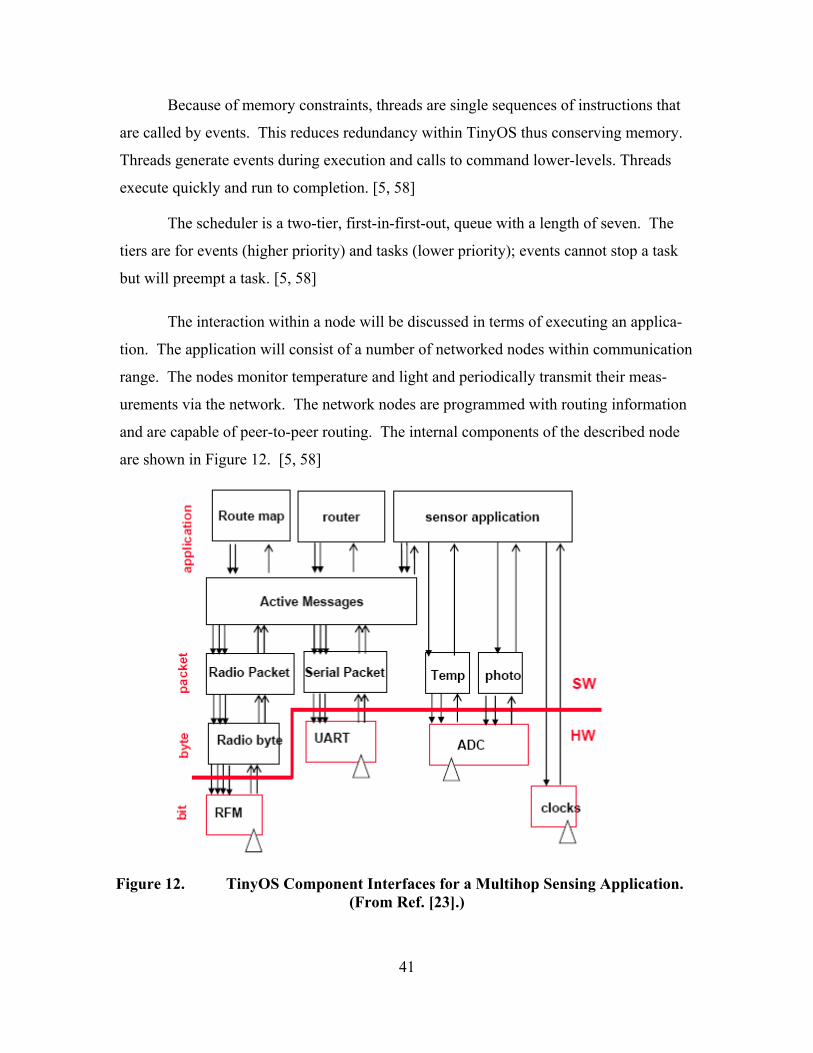
41

Because of memory constraints, threads are single sequences of instructions that

are called by events. This reduces redundancy within TinyOS thus conserving memory.

Threads generate events during execution and calls to command lower-levels. Threads

execute quickly and run to completion. [5, 58]

The scheduler is a two-tier, first-in-first-out, queue with a length of seven. The

tiers are for events (higher priority) and tasks (lower priority); events cannot stop a task

but will preempt a task. [5, 58]

The interaction within a node will be discussed in terms of executing an applica-

tion. The application will consist of a number of networked nodes within communication

range. The nodes monitor temperature and light and periodically transmit their meas-

urements via the network. The network nodes are programmed with routing information

and are capable of peer-to-peer routing. The internal components of the described node

are shown in Figure 12. [5, 58]

Figure 12. TinyOS Component Interfaces for a Multihop Sensing Application.

(From Ref. [23].)

42

The application must service the network and the sensors. Each of these in-

put/output devices is represented by a vertical component stack. The application layer

ties the stacks together. An active message contains handler identifiers in each message.

The networking layer implements the appropriate handler when the message arrives.

This is analogous to events being signaled by the application. Application data are

broadcast as a fixed-length active message. If the receiver is an intermediate node be-

tween the BS and the destination, the message handler begins retransmission. Once at the

BS, the handler forwards the packet for execution. [58]

During execution, a timer event is employed to periodically begin data collection.

Once the sensor data are collected, the application employs the send_message command

to start a transfer. The send_message command records the message location and sched-

ules a thread to direct the transmission. Upon execution, the thread assembles a packet

and starts a chain of commands by calling TX_byte within the Radio Byte component.

This call begins the byte-by-byte transmission. When the byte transmission completes,

the Radio Byte will transmit the TX_bit_evt to the packet level controller through the

TX_byte_done event. Once all of a packet’s bytes are transmitted, the packet level cues

the TX_packet_done event, which in turn propagates to the application through the

msg_end_done event. [58]

At times when the node is active, but no transmissions are occuring, the Radio

Frequency Modulator (RFM) component signals the Radio Byte component. When a

start sequence is detected, the transmission process is reserved. The components convert

bits into bytes and bytes into packets. Each component actively signals the higher level.

Once a packet is assembled, the address is verified and the appropriate handler is imple-

mented if a local address match is found. [58]

2. nesC: a Programming Language for Embedded Systems

The TinyOS system, libraries, and applications are written in nesC, a new lan-

guage for programming structured component-based applications. The nesC language is

primarily intended for embedded systems, such as sensor networks. The syntax of nesC

is similar to C, but supports the TinyOS concurrency model, in addition to mechanisms

for structuring, naming, and linking together software components into robust network

components that can be easily composed into complete, concurrent systems.

43

D. EXPERIMENTAL NETWORK HIERARCHICAL DESCRIPTION

A wireless sensor network is an n-dimensional array of a variety of sensor types

and nodes, interconnected by a communications network. Sensor data are shared among

the sensors. Sensor networks are predominantly data centric, rather than address centric.

Queries are directed to a region containing a cluster of sensors organized by a common

coordinator, rather than specific sensor addresses. Aggregation of data can be performed

locally, given the similarity of information from a given cluster, which reduces the net-

work bandwidth demands by transmitting fewer packets. A network hierarchy and clus-

tering of sensor nodes allows for network scalability, self-organization, concurrency of

operation and lower power. This section describes the combination of the IEEE 802.15.4

standard with hardware and software components for wireless sensor network design.

This design was used during experimental and testing phases of this work. [59]

1. Architecture The prototype network was organized for peer-to-peer communications. The net-

work coordinator was statically determined and programmed as the node connected to the

gateway (see Figure 13). This framework is best described as a peered cluster where

nodes can choose a peer (other nodes) to forward transmissions to the gateway (cluster

head). The nodes’ network identification is preprogrammed. The network consisted of

one network coordinator, Node 0, and three sensing nodes, Node 1 through Node 3. All

nodes were capable of operating in full function mode and were programmed with the

same group identifier. Node 0 is attached to the cluster head.

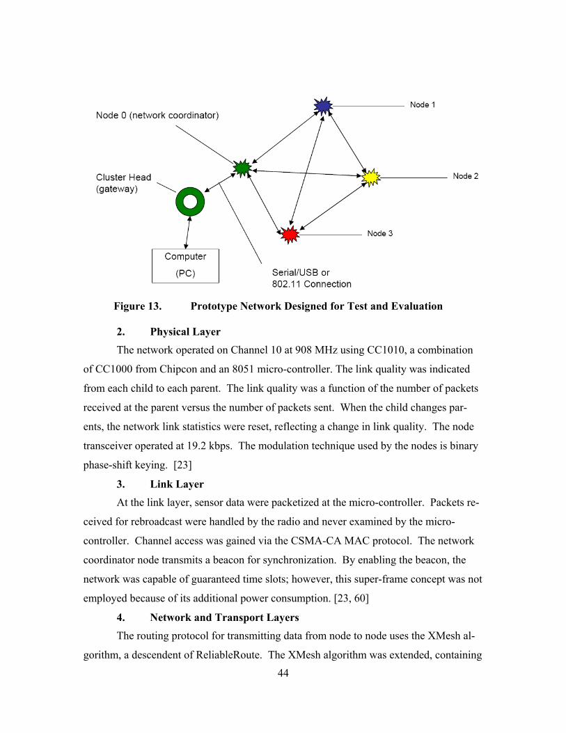
44

Figure 13. Prototype Network Designed for Test and Evaluation 2. Physical Layer The network operated on Channel 10 at 908 MHz using CC1010, a combination

of CC1000 from Chipcon and an 8051 micro-controller. The link quality was indicated

from each child to each parent. The link quality was a function of the number of packets

received at the parent versus the number of packets sent. When the child changes par-

ents, the network link statistics were reset, reflecting a change in link quality. The node

transceiver operated at 19.2 kbps. The modulation technique used by the nodes is binary

phase-shift keying. [23]

3. Link Layer

At the link layer, sensor data were packetized at the micro-controller. Packets re-

ceived for rebroadcast were handled by the radio and never examined by the micro-

controller. Channel access was gained via the CSMA-CA MAC protocol. The network

coordinator node transmits a beacon for synchronization. By enabling the beacon, the

network was capable of guaranteed time slots; however, this super-frame concept was not

employed because of its additional power consumption. [23, 60]

4. Network and Transport Layers The routing protocol for transmitting data from node to node uses the XMesh al-

gorithm, a descendent of ReliableRoute. The XMesh algorithm was extended, containing

45

provisions for link acknowledgement, low power and time synchronization [24]. The

XMesh message packet has an eight-byte preamble to aid in synchronization, a two-byte

synchronizer, and a 36-byte message. [23]

In wireless sensor networks, the traditional transport layer characteristics are not

segregated. Connections are established from child to parent and are terminated when an

application is complete. Error recovery and flow control are not possible because of a

nodes’ limited memory, thus end-to-end reliability is not assured. Packets are thirty-six

bytes long and segmentation and reassembly are not required. [23]

The final component in the network was a bridge, gateway, or cluster head. The

MIB510 gateway from Crossbow functioned as a cluster head and communicated be-

tween the network coordinator and the PC. The PC compiled the sensed data for all as-

sociated nodes. The cluster head has a serial port connection and connects to a computer

through a serial or USB port. The cluster head was capable of supporting data rates of

57.6 kbps. The Stargate gateway, from Crossbow, was also used as a cluster head and

enabled remote connection to the wireless sensor network via the IEEE 802.11 PCMICA

interface. [56-57]

5. Application Layer

Multiple types of sensors can be integrated into a network of nodes. The Mote

Sensor Modules (MTS) used in this network contain various sensor interfaces that are

available through a 51-pin connector. This connector links the MTS to the mote proces-

sor radio (MPR). The MTS310 Multipurpose Sensor Board from Crossbow was deployed

with the motes to form the application layer. The sensors available were magnetic sen-

sor, acceleration sensor, acoustic, temperature, light and a sounder for localization. [40]

6. Software Components Mote-View provides tools, so the user can visualize the stored results from a wire-

less network. Mote-View can support a number of firmware applications running on the

network of motes. This network design used XMesh to enable XListen, a command line

data logging tool, that parses the information received from the motes into user friendly

format. Mote-View provides a graphic user interface to aid in data visualization. The

nodes were programmed with Surge-Reliable, a network statistics program. Surge-

Reliable was used to evaluate radio range. Nodes were reprogrammed with XMTS310, a

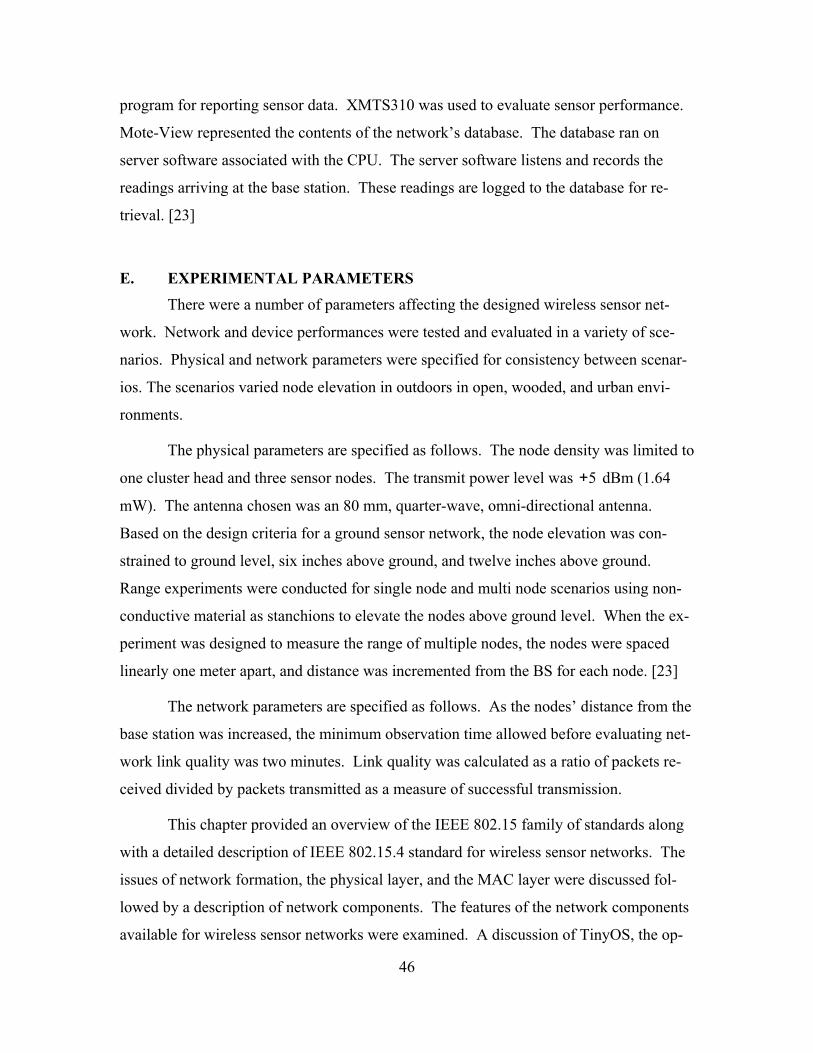
46

program for reporting sensor data. XMTS310 was used to evaluate sensor performance.

Mote-View represented the contents of the network’s database. The database ran on

server software associated with the CPU. The server software listens and records the

readings arriving at the base station. These readings are logged to the database for re-

trieval. [23]

E. EXPERIMENTAL PARAMETERS There were a number of parameters affecting the designed wireless sensor net-

work. Network and device performances were tested and evaluated in a variety of sce-

narios. Physical and network parameters were specified for consistency between scenar-

ios. The scenarios varied node elevation in outdoors in open, wooded, and urban envi-

ronments.

The physical parameters are specified as follows. The node density was limited to

one cluster head and three sensor nodes. The transmit power level was 5+ dBm (1.64

mW). The antenna chosen was an 80 mm, quarter-wave, omni-directional antenna.

Based on the design criteria for a ground sensor network, the node elevation was con-

strained to ground level, six inches above ground, and twelve inches above ground.

Range experiments were conducted for single node and multi node scenarios using non-

conductive material as stanchions to elevate the nodes above ground level. When the ex-

periment was designed to measure the range of multiple nodes, the nodes were spaced

linearly one meter apart, and distance was incremented from the BS for each node. [23]

The network parameters are specified as follows. As the nodes’ distance from the

base station was increased, the minimum observation time allowed before evaluating net-

work link quality was two minutes. Link quality was calculated as a ratio of packets re-

ceived divided by packets transmitted as a measure of successful transmission.

This chapter provided an overview of the IEEE 802.15 family of standards along

with a detailed description of IEEE 802.15.4 standard for wireless sensor networks. The

issues of network formation, the physical layer, and the MAC layer were discussed fol-

lowed by a description of network components. The features of the network components

available for wireless sensor networks were examined. A discussion of TinyOS, the op-

47

erating system used for wireless sensor networks, was presented, and an overview of its

programming language, nesC was provided. Investigation into the characteristics of a

wireless sensor network and the dominant standards has led to an experimental network

as described in this chapter. The experimental results from the evaluation of the proto-

type network follows in the next chapter.

48


49

IV. EXPERIMENTAL RESULTS

This chapter discusses the results from experiments designed to evaluate the per-

formance of the wireless sensor network described in Chapter III. The experiments are

categorized into communication ranges, sensing ranges and network performance. The

experimental results were obtained through numerous deployments of MICA2 motes in

various scenarios. The radio range was measured indoor and outdoor. The sensing range

experiments focused on acoustic, magnetic, and acceleration sensing. Detection and

tracking tests were conducted using the acoustic sensor and the magnetic sensor. The

network performance was calculated from measurements compiled during the radio range

experiments.

A. RADIO RANGE TEST Factors influencing the communication capability of a MICA2 mote are transmis-

sion power, antenna length, node elevation and effects of multi-path. The radio range

experiment focused on the effects of multi-path and the relation to range and node eleva-

tion. The transmission power and antenna gain were held constant.

The plots of experimental results depict link quality. Link quality is a ratio of

number of packets received divided by number of packets transmitted; specified in the

results reported here as a percentage. The plots depict link quality percentage on the y-

axis and distance from the cluster head in meters on the x-axis.

Figure 14 describes the physical topology of the network for single node and mul-

ti-node experiments. The cluster head, depicted in green, is a gateway device with Node

0 attached. The section begins with the results from open terrain range experiments.

These results are followed by results from forested terrain, urban street, and indoor ex-

periments.

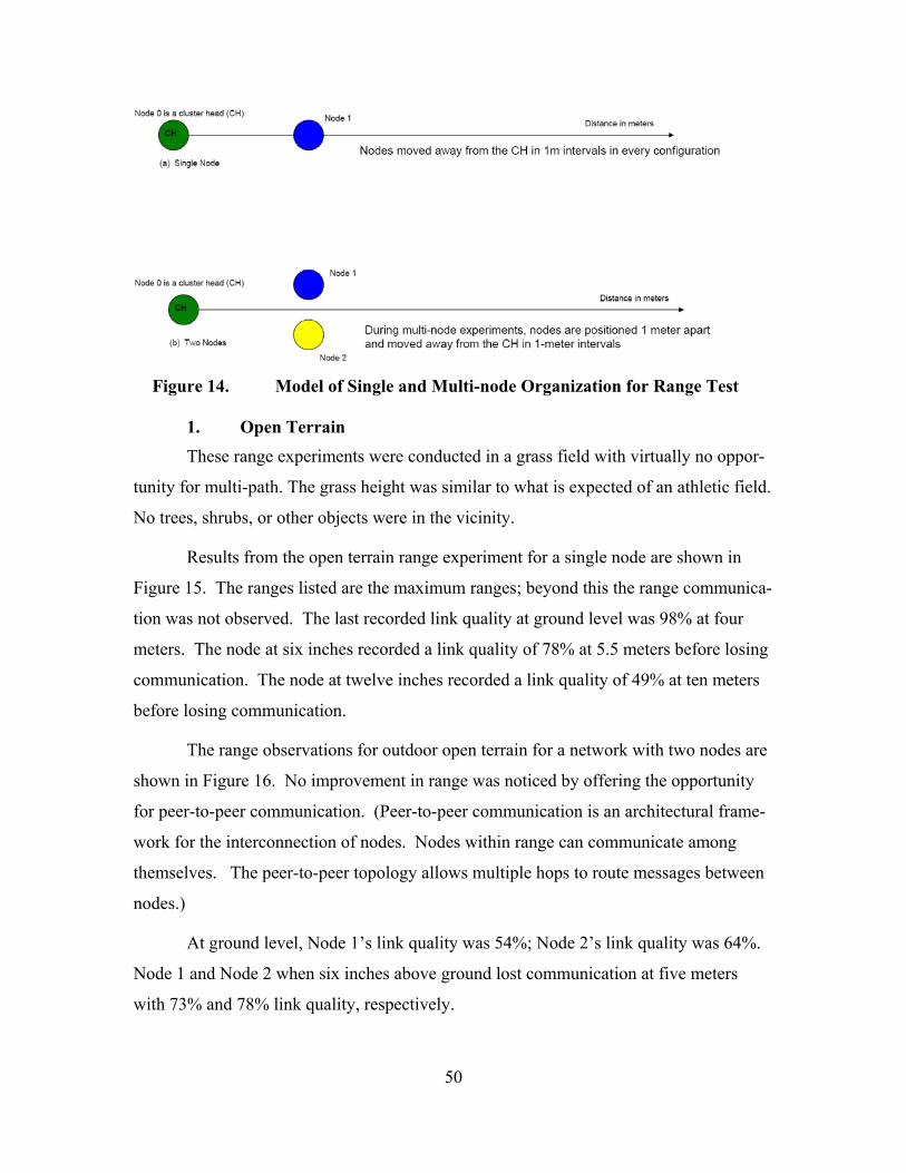
50

Figure 14. Model of Single and Multi-node Organization for Range Test

1. Open Terrain These range experiments were conducted in a grass field with virtually no oppor-

tunity for multi-path. The grass height was similar to what is expected of an athletic field.

No trees, shrubs, or other objects were in the vicinity.

Results from the open terrain range experiment for a single node are shown in

Figure 15. The ranges listed are the maximum ranges; beyond this the range communica-

tion was not observed. The last recorded link quality at ground level was 98% at four

meters. The node at six inches recorded a link quality of 78% at 5.5 meters before losing

communication. The node at twelve inches recorded a link quality of 49% at ten meters

before losing communication.

The range observations for outdoor open terrain for a network with two nodes are

shown in Figure 16. No improvement in range was noticed by offering the opportunity

for peer-to-peer communication. (Peer-to-peer communication is an architectural frame-

work for the interconnection of nodes. Nodes within range can communicate among

themselves. The peer-to-peer topology allows multiple hops to route messages between

nodes.)

At ground level, Node 1’s link quality was 54%; Node 2’s link quality was 64%.

Node 1 and Node 2 when six inches above ground lost communication at five meters

with 73% and 78% link quality, respectively.

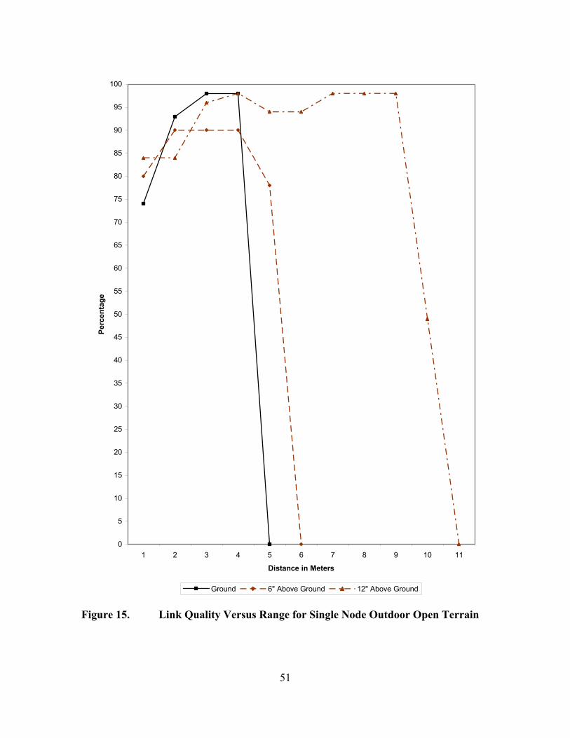
51

0

5

10

15

20

25

30

35

40

45

50

55

60

65

70

75

80

85

90

95

100

1 2 3 4 5 6 7 8 9 10 11

Distance in Meters

Perc

enta

ge

Ground 6" Above Ground 12" Above Ground

Figure 15. Link Quality Versus Range for Single Node Outdoor Open Terrain

52

Figure 16. Link Quality Versus Range for a Two Sensor Node Network in Out-door Open Terrain

Nodes at twelve inches maintained communication at ten meters by peering. The

link quality of the node communicating with the CH was 67%. For nodes at twelve

inches, Node 2 changed its parent at ten meters and began peer-to-peer communication

with Node 1. Nodes at ground level and those at six inches remained parented with the

CH.

0

5

10

15

20

25

30

35

40

45

50

55

60

65

70

75

80

85

90

95

100

1 2 3 4 5 6 7 8 9 10 11

Distance in Meters

Perc

enta

ge

Ground 6" Above Ground 12" Above Ground

53

Measurements of network communication ranges were consistent between the

single node and the multi-node experiments while the link quality measurements

changed. The link quality for nodes at ground level degraded between the single node

and the multi-node experiments. This degradation is attributed to radio frequency inter-

ference. The nodes at six inches did not experience an appreciable change. The nodes at

twelve inches experienced improved link quality at maximum communication range.

This is attributed to the nodes establishing a peer-to-peer connection rather than compet-

ing for access to the base station.

2. Outdoor Wooded This scenario was conducted in a wooded area with trees spaced five to eight feet

apart. The trees were predominantly pines with trunk diameters of six to eight inches.

Pine needles were prevalent on the forest floor as ground cover. The area had small un-

dergrowth vegetation spaced ten to twelve feet apart. The results for single node range

test in a wooded environment are shown in Figure 17.

The single-node experiment revealed that nodes at ground level maintained trans-

mission up to five meters with at least 90% link quality, and failed to communicate be-

yond five meters. The nodes placed at six and twelve inches above the ground main-

tained communications up to nine meters from the CH; beyond nine meters, reliable

communication was not established. At maximum range, the link quality achieved for

the node at six inches was 90%, and for the node at twelve inches was 85%.

In comparison to open terrain, the node at ground level’s range improved one me-

ter with no appreciable difference in link quality. In comparison to open terrain, the node

at the six-inch range improved from 5.5 meters to 9 meters, and link quality improved

from 78% to 90%. A node at a twelve-inch range decreased by one meter to nine meters,

and the link quality was unchanged.

Multiple-node range performances in a wooded environment are shown in Figure

18. In comparison to a single-node case, the ground range improved by three meters,

while link quality degraded 12%. Performance at six inches above the ground remained

unchanged with the opportunity for peering. The nodes twelve inches above the ground

achieved maximum communication range at twelve meters, a three-meter improvement

54

over single node measurements. At twelve inches, one of the nodes often experienced

unusually high link quality. This resulted from a peer-to-peer association.

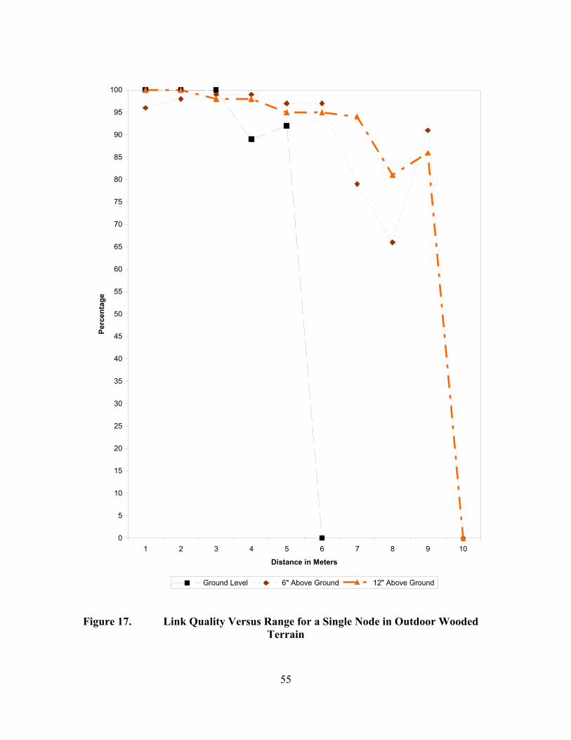
55

0

5

10

15

20

25

30

35

40

45

50

55

60

65

70

75

80

85

90

95

100

1 2 3 4 5 6 7 8 9 10

Distance in Meters

Perc

enta

ge

Ground Level 6" Above Ground 12" Above Ground

Figure 17. Link Quality Versus Range for a Single Node in Outdoor Wooded Terrain

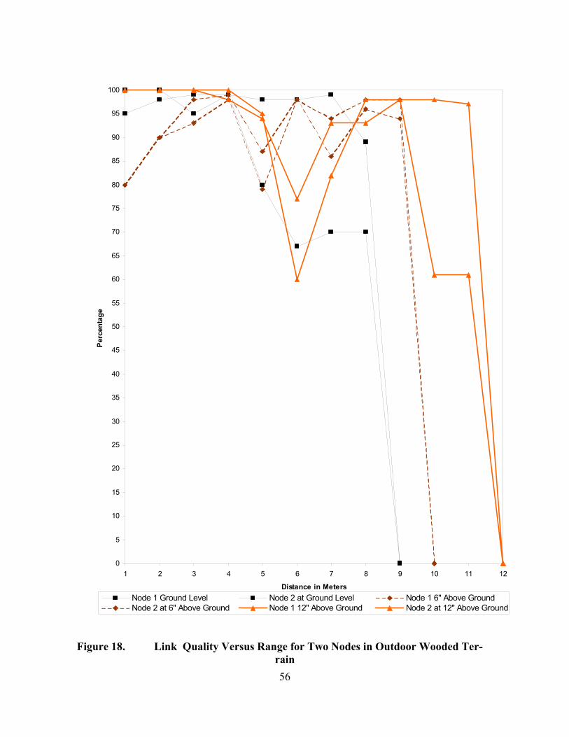
56

0

5

10

15

20

25

30

35

40

45

50

55

60

65

70

75

80

85

90

95

100

1 2 3 4 5 6 7 8 9 10 11 12

Distance in Meters

Perc

enta

ge

Node 1 Ground Level Node 2 at Ground Level Node 1 6" Above GroundNode 2 at 6" Above Ground Node 1 12" Above Ground Node 2 at 12" Above Ground

Figure 18. Link Quality Versus Range for Two Nodes in Outdoor Wooded Ter-rain

57

The link quality in open terrain degraded gradually. For wooded terrain, the link

quality was somewhat erratic. This can be attributed to more opportunity for multi-path

effects of diffusion, absorption, and reflection in a wooded environment. In comparison

to open terrain, diffusion and absorption negatively impacted link quality while reflection

had a positive impact on range, which improved at each elevation.

3. Urban Outdoor

The urban scenario included many energy-diffusing objects. The urban street was

two-lane asphalt with concrete curbs, sidewalks and metal lampposts. It was fronted on

one side by a three-story brick building and on the other side by residential homes with

foliage bordering the sidewalk. One lane of traffic was blocked off and the nodes were

placed in the center of that lane. Vehicle traffic was light and sporadic resulting in no

significant enhancement or degradation of range or link quality.

Results for the single-node scenario are shown in Figure 19. At ground level,

communication with the CH was lost at three meters. Because of the sharp contrast and

departure from previous results, the node was incremented from 3 meters to 3.5 meters.

At 3.5 meters, the node’s link quality was 89%. This link quality remained consistent at

3.75 meters. The node was unable to communicate with the BS from 4 meters to 5.5 me-

ters. At 5.5 meters the link quality was 63% and the node maintained communication at

6 meters. Beyond six meters, communication was unobserved and attempts were termi-

nated after a range of nine meters. The node at six inches maintained communications

until eight meters with last reported link quality of 65%. An interesting result from this

scenario is the sharp drop in link quality at two meters. The node at twelve inches lost

communication beyond thirteen meters where reported link quality was 58%.

Compared to open and wooded terrain scenarios, the ground level null at three

meters was uncharacteristic. At ground level, communication beyond four meters was

uncharacteristic. The four-meter range increase at a twelve-inch elevation was also un-

characteristic. These changes can be attributed to the urban environment; absorption and

diffusion created electromagnetic nulls, and reflection improved range.

The urban street scenario for two nodes meets with slightly different results com-

pared to the single node case (see Figure 20). The nodes at ground level were able to

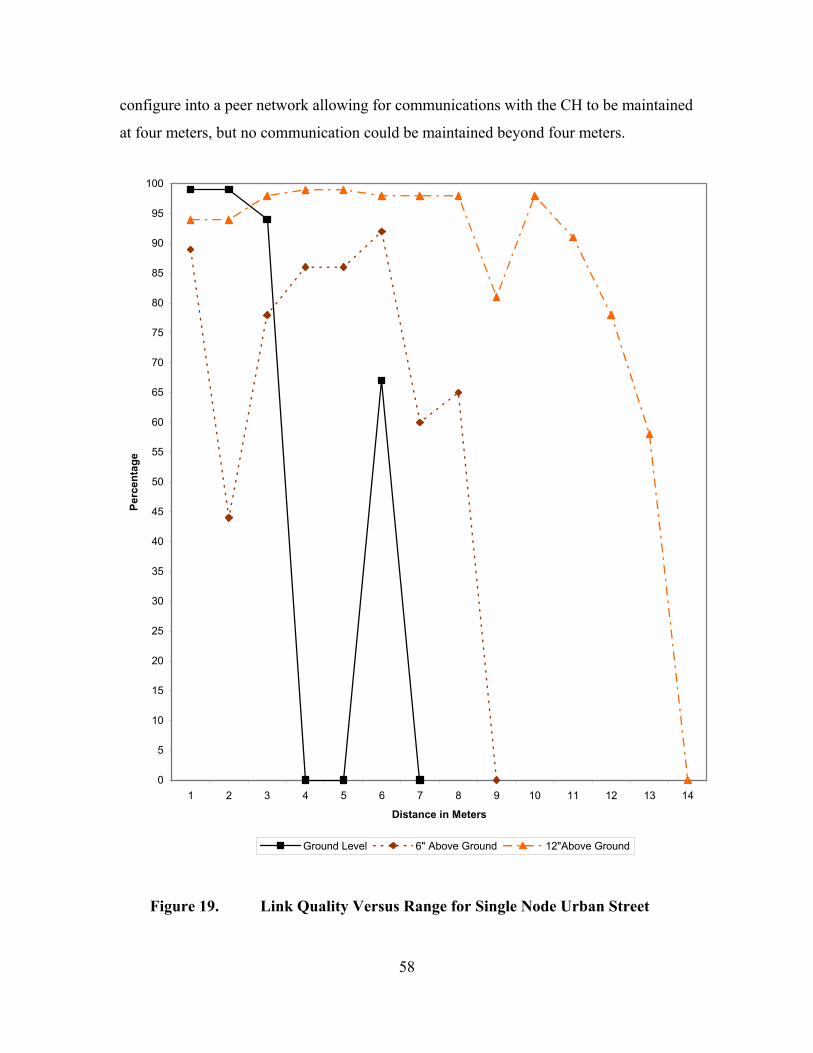
58

configure into a peer network allowing for communications with the CH to be maintained

at four meters, but no communication could be maintained beyond four meters.

0

5

10

15

20

25

30

35

40

45

50

55

60

65

70

75

80

85

90

95

100

1 2 3 4 5 6 7 8 9 10 11 12 13 14

Distance in Meters

Perc

enta

ge

Ground Level 6" Above Ground 12"Above Ground

Figure 19. Link Quality Versus Range for Single Node Urban Street

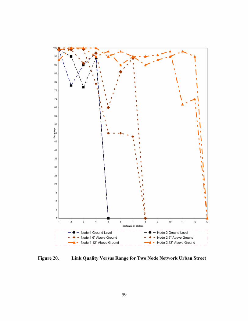
59

0

5

10

15

20

25

30

35

40

45

50

55

60

65

70

75

80

85

90

95

100

1 2 3 4 5 6 7 8 9 10 11 12 13

Distance in Meters

Perc

enta

ge

Node 1 Ground Level Node 2 Ground LevelNode 1 6" Above Ground Node 2 6" Above GroundNode 1 12" Above Ground Node 2 12" Above Ground

Figure 20. Link Quality Versus Range for Two Node Network Urban Street

60

The nodes at six inches of elevation experienced significant link degradation at five me-

ters. The nodes re-associated in a peering manner, and the link quality improved for

Node 1 which peered with Node 2. Node 2’s link quality to the CH did not improve.

The nodes maintained peered communication with the CH until eight meters where

communication for both nodes was lost. Node 1’s link quality to its peer was 95%; Node

2’s link quality to the CH was 48%. A similar trend was observed for nodes at twelve

inches. The nodes peered at seven meters, thus improving the quality of communication

for both nodes. The peered relationship was maintained until thirteen meters beyond

which communication with the CH was not observed. The link quality for the node at

twelve inches communicating with the CH was fifty-eight percent at thirteen meters.

Results demonstrated the diverse effects of the network’s environment. Range

improvements at twelve inches from the single-node experiment were not observed in the

multi-node experiment where results were more consistent with scenarios in open and

wooded terrain.

The outdoor urban experiment was repeated with a node multiple of three. The

ability for multiple peering opportunities marginally improved range performance at

ground level, and no change was observed for nodes at six and twelve inches above

ground. Nodes at ground level improved their communication range from four meters to

six meters.

4. Indoor The experiments for an indoor environment were completed in a two-story ban-

quet room (20' 60') × with two walls of concrete, one wall of glass windows, and one

wall of concrete with glass windows. Concrete pillars lined both sides of the room. The

floor was tile over concrete.

The results of indoor range experiments for single node are shown in Figure 21.

The node at ground level lost communication at three meters with a link quality of 92%.

Incrementing by intervals shorter than one meter did not reestablish communication. The

node at six inches lost communication at nine meters with a link quality of 74% and, once

again, a smaller interval for range increment was unsuccessful in maintaining communi-

cations. The node at twelve inches lost communication at ten meters. An increment of

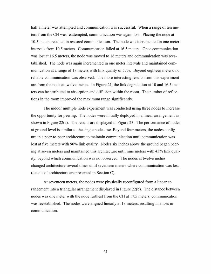
61

half a meter was attempted and communication was successful. When a range of ten me-

ters from the CH was reattempted, communication was again lost. Placing the node at

10.5 meters resulted in restored communication. The node was incremented in one meter

intervals from 10.5 meters. Communication failed at 16.5 meters. Once communication

was lost at 16.5 meters, the node was moved to 16 meters and communication was rees-

tablished. The node was again incremented in one meter intervals and maintained com-

munication at a range of 18 meters with link quality of 57%. Beyond eighteen meters, no

reliable communication was observed. The more interesting results from this experiment

are from the node at twelve inches. In Figure 21, the link degradation at 10 and 16.5 me-

ters can be attributed to absorption and diffusion within the room. The number of reflec-

tions in the room improved the maximum range significantly.

The indoor multiple node experiment was conducted using three nodes to increase

the opportunity for peering. The nodes were initially deployed in a linear arrangement as

shown in Figure 22(a). The results are displayed in Figure 23. The performance of nodes

at ground level is similar to the single node case. Beyond four meters, the nodes config-

ure in a peer-to-peer architecture to maintain communication until communication was

lost at five meters with 90% link quality. Nodes six inches above the ground began peer-

ing at seven meters and maintained this architecture until nine meters with 43% link qual-

ity, beyond which communication was not observed. The nodes at twelve inches

changed architecture several times until seventeen meters where communication was lost

(details of architecture are presented in Section C).

At seventeen meters, the nodes were physically reconfigured from a linear ar-

rangement into a triangular arrangement displayed in Figure 22(b). The distance between

nodes was one meter with the node furthest from the CH at 17.5 meters; communication

was reestablished. The nodes were aligned linearly at 18 meters, resulting in a loss in

communication.

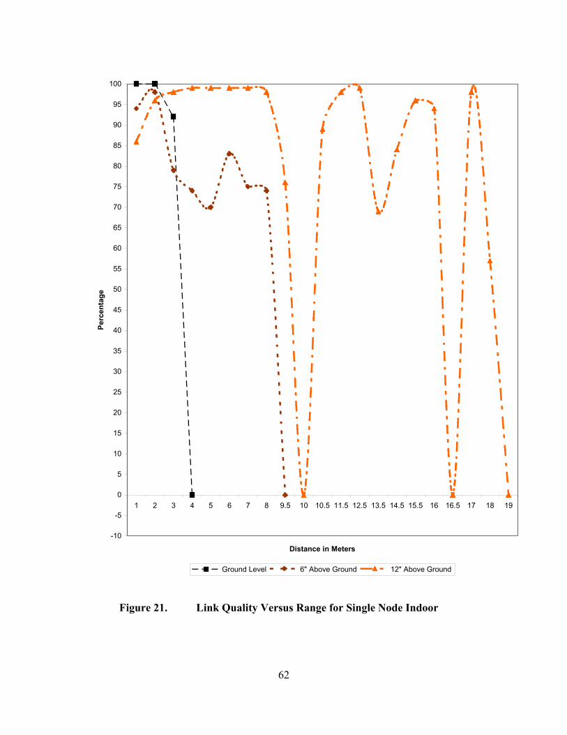
62

-10

-5

0

5

10

15

20

25

30

35

40

45

50

55

60

65

70

75

80

85

90

95

100

1 2 3 4 5 6 7 8 9.5 10 10.5 11.5 12.5 13.5 14.5 15.5 16 16.5 17 18 19

Distance in Meters

Perc

enta

ge

Ground Level 6" Above Ground 12" Above Ground

Figure 21. Link Quality Versus Range for Single Node Indoor

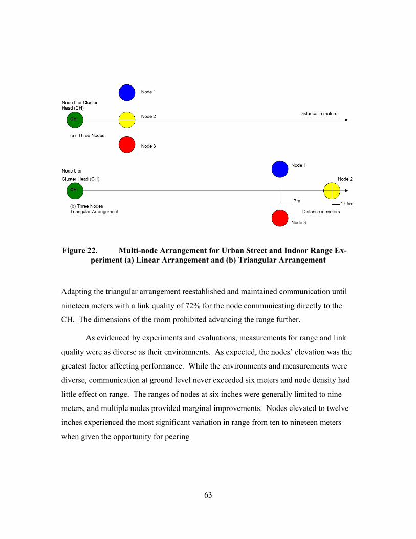
63

Figure 22. Multi-node Arrangement for Urban Street and Indoor Range Ex-periment (a) Linear Arrangement and (b) Triangular Arrangement

Adapting the triangular arrangement reestablished and maintained communication until

nineteen meters with a link quality of 72% for the node communicating directly to the

CH. The dimensions of the room prohibited advancing the range further.

As evidenced by experiments and evaluations, measurements for range and link

quality were as diverse as their environments. As expected, the nodes’ elevation was the

greatest factor affecting performance. While the environments and measurements were

diverse, communication at ground level never exceeded six meters and node density had

little effect on range. The ranges of nodes at six inches were generally limited to nine

meters, and multiple nodes provided marginal improvements. Nodes elevated to twelve

inches experienced the most significant variation in range from ten to nineteen meters

when given the opportunity for peering

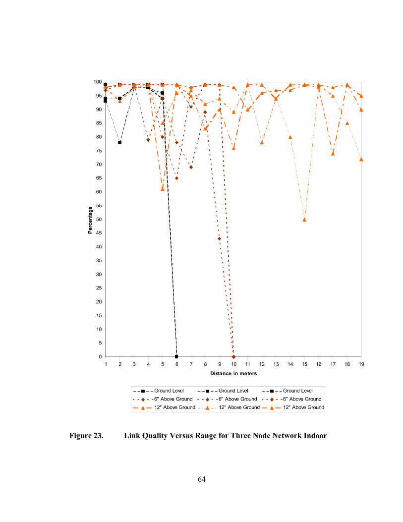
64

0

5

10

15

20

25

30

35

40

45

50

55

60

65

70

75

80

85

90

95

100

1 2 3 4 5 6 7 8 9 10 11 12 13 14 15 16 17 18 19

Distance in meters

Perc

enta

ge

Ground Level Ground Level Ground Level6" Above Ground 6" Above Ground 6" Above Ground12" Above Ground 12" Above Ground 12" Above Ground

Figure 23. Link Quality Versus Range for Three Node Network Indoor

65

B. SENSOR RANGE TEST

The sensor subsystem was tested for range. Because of the unique aspects of each

sensor, specific scenarios were designed based on potential applications. The acoustic,

magnetic, and acceleration sensors were selected for testing. The acoustic sensor was

tested in a noise-free environment, in an urban market, and outdoors. The magnetic sen-

sor tests attempted to establish parameters for object size relative to distance from the

sensor and to monitor vehicular traffic. The acceleration sensor scenario was designed to

measure responses to vibration and response to motion.

1. Acoustic Sensor The test of the acoustic sensor was initially conducted in an indoor area similar to

the food court in many shopping centers. The microphone could detect sounds tens of

meters away but because of the chaotic nature, reliable estimations of performance were

not achieved. The acoustic readings could not be directly attributed to a specific source

because of the multitude of competing sounds. The acoustic sensor was then placed in a

noise-free room. A news program was played at conversational tone. The sensor node

was moved around the room and recordings were documented. The sensors’ ability to

detect acoustic variations in this environment was restricted to eight meters with a

180 field of view. Beyond eight meters, the human voice was not distinguishable from

ambient noise.

A test to determine the suitability of using the acoustic sensor for aircraft tracking

was conducted. A sensor field was established approximately one quarter mile from the

end of the runway. The sensor field was established in open terrain along the aircrafts’

flight path for takeoff and landing. The acoustic signal recorded by one of these sensors

is shown in Figure 24; other sensors recorded similar results. The y-axis represents the

difference in decibels between ambient noise and measured values. The x-axis represents

time scale with each marker representing eight seconds (the time between node transmis-

sions). The three spikes correspond to the aircraft passing overhead after takeoff. The

first and second spikes were jet aircraft. The first was a commercial jet and the second a

smaller private jet. The third spike corresponds to a twin engine turboprop during take-

off. The first and third aircraft passed approximately 120 feet overhead. The second air-

craft passed overhead at a higher but undetermined altitude. The sharp drops after the jet

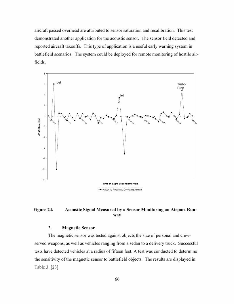
66

aircraft passed overhead are attributed to sensor saturation and recalibration. This test

demonstrated another application for the acoustic sensor. The sensor field detected and

reported aircraft takeoffs. This type of application is a useful early warning system in

battlefield scenarios. The system could be deployed for remote monitoring of hostile air-

fields.

Figure 24. Acoustic Signal Measured by a Sensor Monitoring an Airport Run-way

2. Magnetic Sensor The magnetic sensor was tested against objects the size of personal and crew-

served weapons, as well as vehicles ranging from a sedan to a delivery truck. Successful

tests have detected vehicles at a radius of fifteen feet. A test was conducted to determine

the sensitivity of the magnetic sensor to battlefield objects. The results are displayed in

Table 3. [23]

67

Table 3. Magnetometer Sensitivity Readings for Personal Weapons, Crew-Served Weapons, and Automobiles

Object Detection Distance in

inches

Magnetometer Differen-

tial in mutual gauss

Pistol 6 11.61

Rifle 12 11.61

Crew-Served Weapon 16 9.59

Automobile (Sedan) 12 12.8

Automobile (Jeep) 14 33.4

Automobile (Sport Utility

Vehicle)

24 76.17

The magnetic sensor successfully detected magnetic field changes for all objects

tested. The sensitivity variations in Table 3 reflect the increase in magnetic field reported

by the magnetic sensor. These values are measured in mutual gauss and reflect the mag-

netic field increase in response to the object’s presence. As expected, the sensor reading

is a function of range and the object’s metallic density. The detection distance for weap-

ons is the largest distance at which the sensor reliably detected the presence of the

weapon. The magnetic sensor readings for rifle and pistol were identical, but the rifle

was detected at a greater distance than the pistol. The same was true for the crew-served

weapon. The results indicate a detection range that is extremely short, which implies that

this particular model of sensor may not be best suited for this application. A magnetic

sensor deployed in a ground sensor network should be able to detect weapons three feet

away. Three feet is the approximate height of weapons when personnel are carrying

them.

An experiment was conducted to classify the vehicle type based on magnetic sen-

sor readings. The experiment was conducted on a two-lane residential road. The results

are displayed in Figure 25 and Table 3. The sensor was placed in the center of one lane

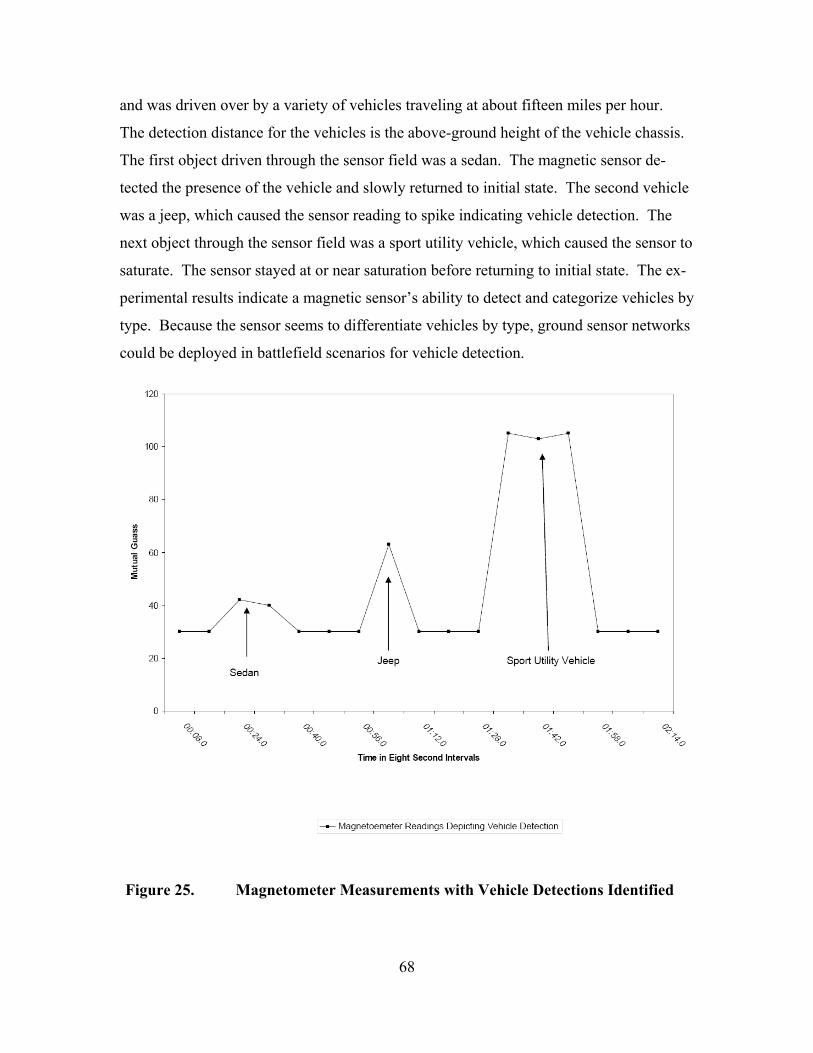
68

and was driven over by a variety of vehicles traveling at about fifteen miles per hour.

The detection distance for the vehicles is the above-ground height of the vehicle chassis.

The first object driven through the sensor field was a sedan. The magnetic sensor de-

tected the presence of the vehicle and slowly returned to initial state. The second vehicle

was a jeep, which caused the sensor reading to spike indicating vehicle detection. The

next object through the sensor field was a sport utility vehicle, which caused the sensor to

saturate. The sensor stayed at or near saturation before returning to initial state. The ex-

perimental results indicate a magnetic sensor’s ability to detect and categorize vehicles by

type. Because the sensor seems to differentiate vehicles by type, ground sensor networks

could be deployed in battlefield scenarios for vehicle detection.

Figure 25. Magnetometer Measurements with Vehicle Detections Identified

69

The utility of a sensor network arises from the aggregation of data. In some in-

stances, merely combining the results of multiple sensors into a single graphical user in-

terface could provide an opportunity for data fusion. Another instance of data fusion is

combining the results of multiple sensors into a single packet of information. A simple

test was conducted to fuse network data by overlapping the results from two magnetic

sensors. The test was an attempt to demonstrate a wireless, ground sensor network’s abil-

ity to detect and track.

Two sensor nodes were deployed four meters apart, at ground level, on a residen-

tial street. The sensors were left in place during which a variety of automobiles passed

over them. The posted speed limit was twenty miles per hour. The results of the mag-

netic sensor measurements demonstrate the ability to detect and track a metal object (see

Figure 26).

Compared to the single node case, inaccuracy and inconsistency were observed.

An apparent inaccuracy results from the nodes reporting once every eight seconds; Node

1 reports vehicle detections sixteen seconds earlier than Node 3. Considering the vehi-

cles’ speed and the distance between nodes, the sixteen seconds between observations

seems inaccurate. An inconsistency exits between the measured values for the sedan and

jeep when compared to the results in Figure 25. While time inaccuracy existed and in-

consistent measured values were observed, the sensor field successfully detected, re-

ported, and tracked vehicle movement.

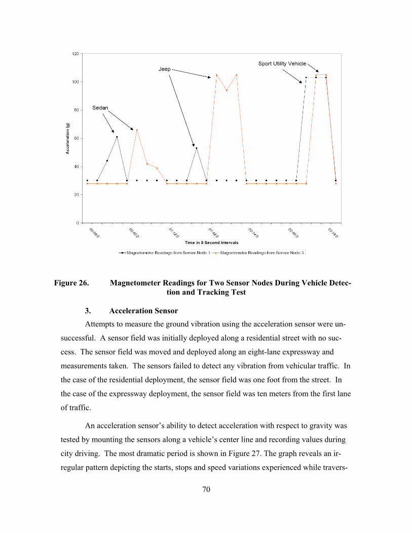
70

Figure 26. Magnetometer Readings for Two Sensor Nodes During Vehicle Detec-tion and Tracking Test

3. Acceleration Sensor Attempts to measure the ground vibration using the acceleration sensor were un-

successful. A sensor field was initially deployed along a residential street with no suc-

cess. The sensor field was moved and deployed along an eight-lane expressway and

measurements taken. The sensors failed to detect any vibration from vehicular traffic. In

the case of the residential deployment, the sensor field was one foot from the street. In

the case of the expressway deployment, the sensor field was ten meters from the first lane

of traffic.

An acceleration sensor’s ability to detect acceleration with respect to gravity was

tested by mounting the sensors along a vehicle’s center line and recording values during

city driving. The most dramatic period is shown in Figure 27. The graph reveals an ir-

regular pattern depicting the starts, stops and speed variations experienced while travers-

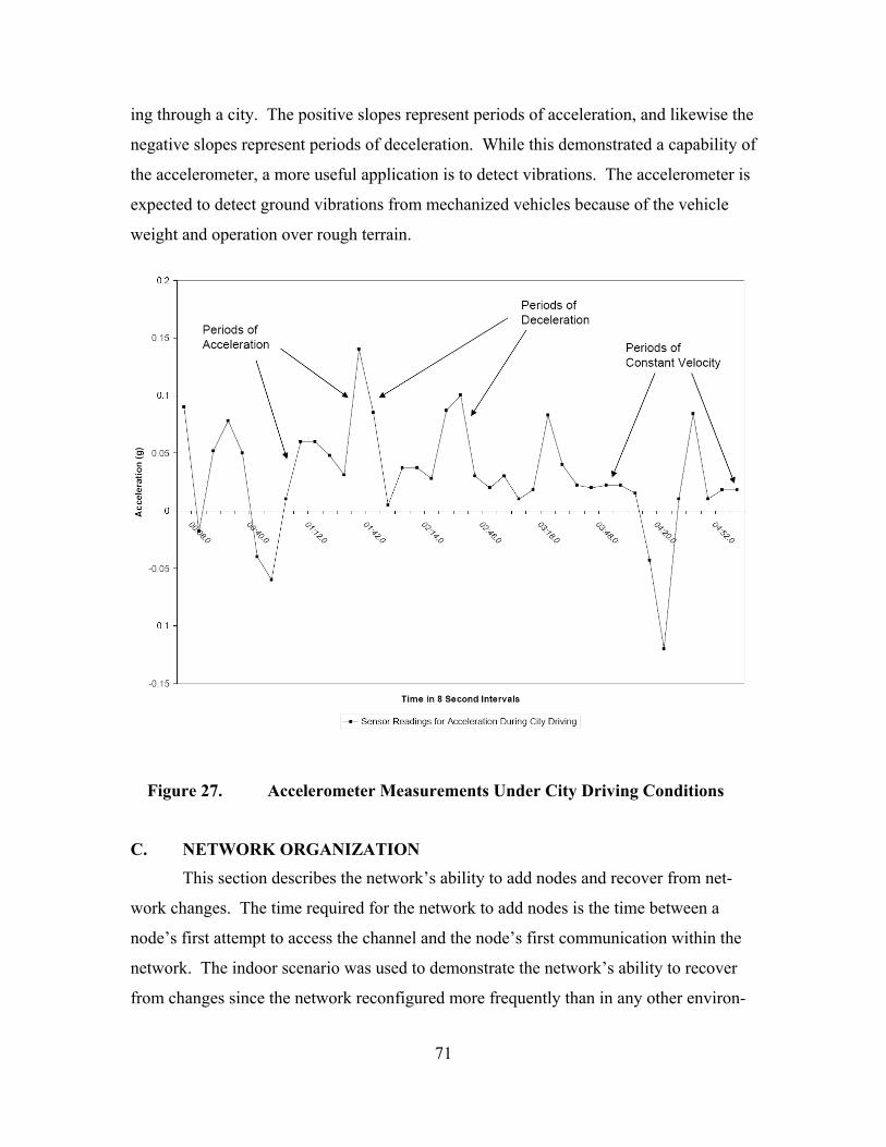
71

ing through a city. The positive slopes represent periods of acceleration, and likewise the

negative slopes represent periods of deceleration. While this demonstrated a capability of

the accelerometer, a more useful application is to detect vibrations. The accelerometer is

expected to detect ground vibrations from mechanized vehicles because of the vehicle

weight and operation over rough terrain.

Figure 27. Accelerometer Measurements Under City Driving Conditions

C. NETWORK ORGANIZATION

This section describes the network’s ability to add nodes and recover from net-

work changes. The time required for the network to add nodes is the time between a

node’s first attempt to access the channel and the node’s first communication within the

network. The indoor scenario was used to demonstrate the network’s ability to recover

from changes since the network reconfigured more frequently than in any other environ-

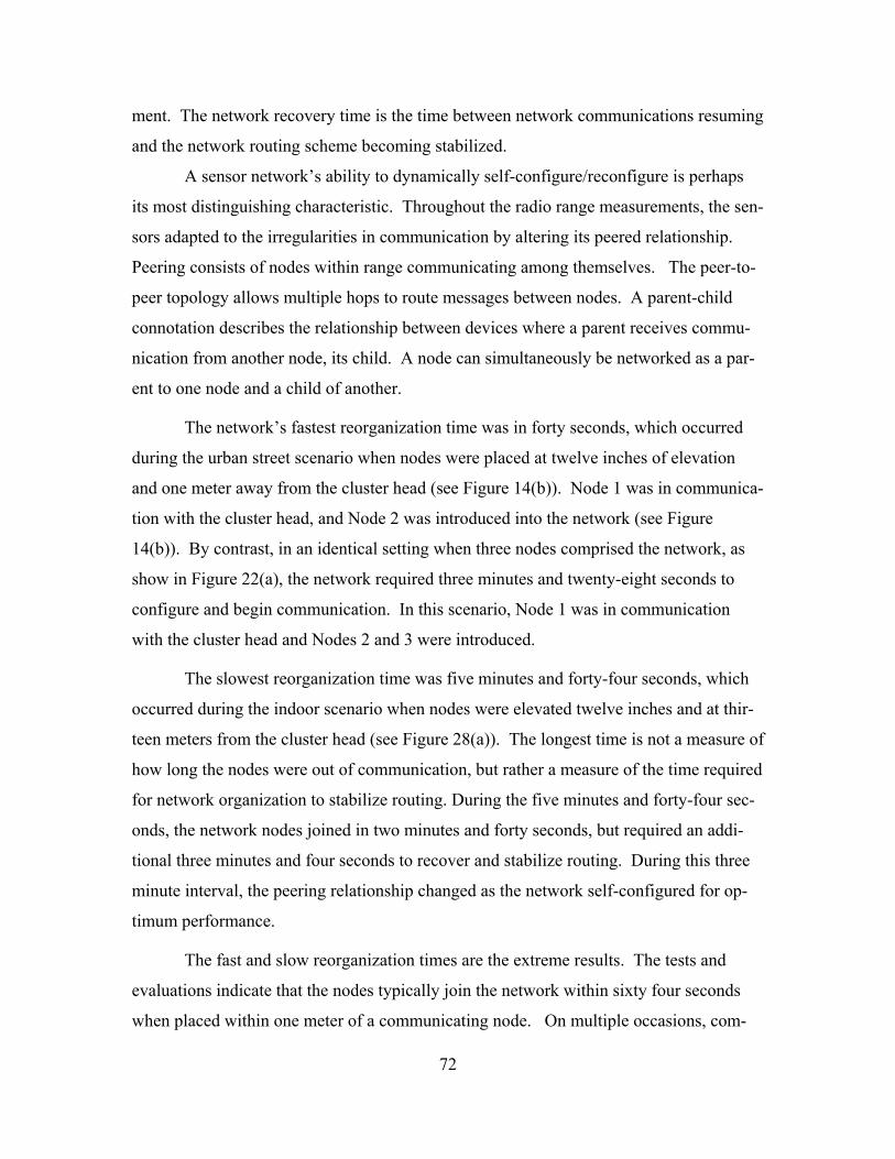
72

ment. The network recovery time is the time between network communications resuming

and the network routing scheme becoming stabilized.

A sensor network’s ability to dynamically self-configure/reconfigure is perhaps

its most distinguishing characteristic. Throughout the radio range measurements, the sen-

sors adapted to the irregularities in communication by altering its peered relationship.

Peering consists of nodes within range communicating among themselves. The peer-to-

peer topology allows multiple hops to route messages between nodes. A parent-child

connotation describes the relationship between devices where a parent receives commu-

nication from another node, its child. A node can simultaneously be networked as a par-

ent to one node and a child of another.

The network’s fastest reorganization time was in forty seconds, which occurred

during the urban street scenario when nodes were placed at twelve inches of elevation

and one meter away from the cluster head (see Figure 14(b)). Node 1 was in communica-

tion with the cluster head, and Node 2 was introduced into the network (see Figure

14(b)). By contrast, in an identical setting when three nodes comprised the network, as

show in Figure 22(a), the network required three minutes and twenty-eight seconds to

configure and begin communication. In this scenario, Node 1 was in communication

with the cluster head and Nodes 2 and 3 were introduced.

The slowest reorganization time was five minutes and forty-four seconds, which

occurred during the indoor scenario when nodes were elevated twelve inches and at thir-

teen meters from the cluster head (see Figure 28(a)). The longest time is not a measure of

how long the nodes were out of communication, but rather a measure of the time required

for network organization to stabilize routing. During the five minutes and forty-four sec-

onds, the network nodes joined in two minutes and forty seconds, but required an addi-

tional three minutes and four seconds to recover and stabilize routing. During this three

minute interval, the peering relationship changed as the network self-configured for op-

timum performance.

The fast and slow reorganization times are the extreme results. The tests and

evaluations indicate that the nodes typically join the network within sixty four seconds

when placed within one meter of a communicating node. On multiple occasions, com-

73

munication was lost by incrementing the node’s range from the cluster head by one me-

ter. Measurements indicate that on those occasions, recovery times varied between two

minutes twenty-four seconds and three minutes and twenty-eight seconds.

Figure 28 displays the network organization and re-association of sensor nodes to

maintain communications during the indoor range test. Figure 28(a) shows the node or-

ganization observed for the range from one meter to thirteen meters. All nodes were chil-

dren of the cluster head. Figure 28(b) displays the first re-organization at fourteen meters

when Node 1 and Node 3 peered with the Node 2. Node 2 remained a child of the cluster

head. The sensor nodes maintained this node organization until fifteen meters. At six-

teen meters, Node 3 re-associated with Node 2 while Nodes 1 and 2 remained children of

the cluster head (see Figure 28(c)). This organization was short lived. At seventeen me-

ters, communication with the cluster head was lost.

74

Figure 28. Illustration of Changes in Network Organization During Indoor Range Test

The physical arrangement of the network was modified into a triangular configu-

ration (see Figure 28(d)), and communication was reestablished. In the triangular ar-

rangement, Node 2 and Node 3 re-associated with Node 1, and Node 1 remained a child

of the cluster head. The network topology changed again at eighteen meters as shown in

Figure 28(b). This was the network organization through nineteen meters when the

physical limitations of room size impeded further testing. Figure 28 graphically depicts

the dynamic nature of the child-parent relationship as the network self-configures for op-

timum performance.

75

D. NETWORK TRAFFIC

The network is characterized by low bit-rate communication because of low

power consumption and small-form factor requirements. This low-bit rate characteristic

has performance implications governing link utilization, throughput and node density,

which are described in this section.

The network bit rate, R, is fixed based on the physical constraints of the devices.

The node’s transceiver is configured to operate at 19.2 kbps at 908 MHz. The cluster

head used transmits to the personal computer at 57.6 kbps (see Figure 13).

The network’s link utilization, node density and throughput are calculated. assum-

ing a transceiver bit rate of 19.2 kbpsR = (with no channel coding), a packet length of

288 bits,L = and transmission interval of int 8 s.t =

The frame length of a packet, framet , defined as the ratio of the number of bits per

packet, L, to the bit rate, R, is given by

.frameLtR

= (4.1)

For this network, 15 msframet = . [14]

The equation for link utilization, U, the fraction of time transmissions occur on a

particular link, is given by

int

frame

frame

tU

t Nt=

− (4.2)

where N is the number of nodes on a particular link. The link utilization for a single node

was 31.8785 10 .−× The utilization rate increased modestly to 31.8856 10−× when three

sensor nodes were on the same link. [14]

Network throughput, T, defined as a product of link utilization and bit rate, is

given by

.T UR= (4.3)

76

For 19.2 kbpsR = and 31.8856 10U −= × , the calculated throughput becomes 36.20 bps or

0.1257 packets per second. [14]

The maximum number of nodes, maxN , by assuming that the link utilization

1,U = is given by

intmax .frame

frame

t tN

t−

= (4.4)

For int 8 st = and 15 msframet = , the maximum number of nodes supported by the link is

max 532.N = For the same bit rate, the number of nodes could be improved by increas-

ing intt , which reduces the duty cycle of the transceiver. The lower duty cycle provides an

additional benefit of extending network lifetime, by consuming less power. While lower

power consumption and increased node density are a benefit of lower duty cycle, the

tradeoff is lower data rate per node.

This chapter presented the results from experiments and tests of wireless ground

sensor networks. Experiments were conducted to determine node range in a variety of

deployment scenarios. Experiments were also conducted to determine the sensing range

for the acoustic sensor, magnetic sensor, and acceleration sensor. The results from detec-

tion and tracking test using the acoustic sensor and the magnetic sensor were described.

Network performance parameters and receiver gain were calculated. Conclusions based

on experimental results follow in the next chapter, along with recommendations for fu-

ture work.

77

V. CONCLUSIONS AND RECOMMENDATIONS

The development of wireless, unattended ground sensor networks has become

feasible with the evolution of integrated circuit technology, wireless communication and

networking. Improvements continue to decrease the size and increase their utility. The

objectives of this thesis were to prototype a wireless, unattended ground sensor network

and to test the node and network performance.

An overview of wireless sensor network characteristics of architecture, protocols

and components led to the selection of IEEE 802.15.4 standard and TinyOS as the tech-

nologies for prototype development. The network consisted of a cluster of three to four

nodes equipped with an acoustic sensor, a magnetic sensor, and an acceleration sensor.

The node and network performance parameters were tested and evaluated. Typical

communication ranges are four meters for nodes at ground level, ten meters for nodes at

six inches above ground, and twelve meters for nodes twelve inches above ground. The

sensors’ range was dependent on the environment and applications. This thesis substanti-

ated the viability of interconnecting, self-organizing sensor nodes in military applications.

The tests and evaluations demonstrated that the network was capable of dynamic adapta-

tion to failure, degradation and tasking.

A. CONCLUSIONS The range performance of sensor networks was directly proportional to the node

elevation and the number of nodes. In a military application, the method of deployment

will govern node elevation. Presence of multiple nodes decreased network re-association

time and improved the opportunity for peered association, thus improving range perform-

ance. A peered association existed when network traffic was multi-hopped to the cluster

head. (The traffic is multi-hopped when a node cannot communicate directly with the

cluster head.)

Results of sensor-range experiments combined with results from the detection and

tracking test established that a sensor node’s coverage could be greater than its communi-

cation range. Sensing range varied by scenario. Due to these diverse observations in per-

78

formance, a priori knowledge of deployment environment improved the accuracy of node

density calculations and network performance estimations.

The characteristics and performance of wireless, unattended ground sensor net-

works demonstrated their suitability for military applications. The system-level evalua-

tion of device communication and sensing range along with network performance de-

tailed in this thesis provide a method to assess the military applicability of wireless, unat-

tended ground sensor networks.

B. RECOMMENDATIONS This thesis employed a prototype wireless, unattended ground sensor network.

The node range performance measurements were conducted at maximum power with an

omni-directional antenna. A recommendation for future research is to evaluate commu-

nication range performance for a variety of antennas and power levels. This work would

improve network designer’s ability to accurately estimate network performance.

A rudimentary fusion of sensor data was achieved by combining the output from

two sensors into a single graphical display. The graphical display demonstrated the abil-

ity to detect and track objects as they traversed through a sensor field. This method was

limited by software tools. A recommendation is to develop software to improve the fu-

sion of sensor data. The cluster head could maintain a database of interest queries and

reporting thresholds. The cluster head would only report information matching these cri-

teria fusing the data from several sensors into one report. This is a more elegant software

technique and offers the same functionality, reduces the network traffic, and alerts users

to significant events

79

APPENDIX INSTALLING TINYOS AND USER INTERFACES

This appendix introduces the procedures for installing TinyOS and some basic

commands for programming the nodes.

TinyOS can be downloaded from the TinyOS website

(http://www.tinyos.net/download.html), through sourceforge’s

http://sourceforge.net/cvs/?group_id=28656) website, or through vendor distribution. It

requires Windows PC (XP or 2000) and 1 GB or more of free disk space in the destina-

tion drive. Other requirements are Acrobat PDF Reader and a means to connect from a

serial port to the PC. The user must log on with administrator privileges.

1. Pre-Check: Uninstall old TinyOS installations if found and ensure that Java is

installed. If Java is not installed, set the path variable to /cygdrive/c/jdk1.4.1-

02/bin/java.

2. Install TinyOS from CDROM provided by Crossbow.

i. Double click on tinyos-1.1.0-1ls.exe inside the TinyOS install folder.

ii. In the “Setup Type” window, select “Complete” and use the default desti-

nation folder. Click on “Next.”

iii. In the “Java License Agreement” window, click “Yes” and then “Next.”

iv. Follow instructions and choose all defaults.

The installation includes:

1. TinyOS and Tools: an event driven OS for wireless sensor networks and tools

for debugging.

2. nesC: an extension of the C language designed for TinyOS.

3. Cygwin: a Linux-like environment for Windows.

4. AVR tools: a suite of software development tolls for Atmel’s AVR proces-

sor.

80

5. Java 1.4 JDK and Java COMM 2.0: for host PC applications and port com-

munications.

6. Graphviz: to view files made from make docs.

The installation will create a directory “tinyos” on the C: drive. The applications can be

found in C:\tinyos\cygwin\opt\tinyos-1.x\apps.

When installation of TinyOS is complete, verify by opening the cygwin window (double

clicking on the cygwin desktop icon). Type toscheck. The last line should say, “toscheck

completed without errors.”

Newer versions of TinyOS are released periodically. The current version and download

instructions can be found at http://www.tinyos.net/scoop/section/Releases. Copy the up-

date into C:\tinyos\cygwin\tmp\, then open the Cygwin window and type:

cd /tmp

rpm --nodeps --force --ignoreos –Uvh tinyos-1.1.<filename copied>

Additonal Installation:

1. Open the cygwin shell and maneuver to the application directory and enter the

application of interest. The applications used during this experiment were in

contrib/xbow/apps directory of tinyos. These contributions are in a zip file called

xbow.tgz.

2. Copy the file xbow.tgz from the TinyOS Updates directory on CDROM to a tem-

porary directory, e.g., C:\tinyos\cygwin\tmp.

3. Open cygwin window and type:

cd /tmp

gunzip xbow.tgz

cd/opt

81

tar –xvf /tmp/xbow.tar

This will unzip Crossbow’s contributions to TinyOS. The contributions include

network applications and testing tools.

4. Once the file is unzipped, the directory can be accessed. Other contributor’s ap-

plications are included and can be entered and installed.

5. Install Surge-View by copying the Surge-View folder on CDROM to the

C:\Program Files\ directory. Surge-View graphically captures network level sta-

tistics and topology.

6. Install a Mote-View by double clicking on the MoteViewSetup.exe. Mote-View is

a graphical user interface designed to display application results. Future versions

of Mote-View are expected to contain the Surge-Reliable application.

a. If the screen Moteview 1.0 setup displaying “The Cygwin release included

in TinyOS 1.1 is required but not installed. You will not be able to log

data locally. Do you want to continue?” appears, click YES.

b. The Mote-View setup wizard will start and complete the installation.

c. If the system is having problems, manually install the database:

i. Open Cygwin

ii. Type startdb to start the database server

iii. Type \q to quit the database client

iv. Type createdb-task to generate database tables

v. If the problem still presists: rm –fr /pgdata

createdb-task

vi. Add a local results table by copying mts310_db from the Cross-

bow cd into c:/tmp and then type:

psql task <mts310_db

Open cygwin and type:

82

pg_dump -f out_file –t table_name task

This sequence will load files into MoteView for data storage.

7. Copy from Misc directory on cdrom pn.exe and terminal.exe to desktop or other

convenient location. pn.exe is Programmer’s Notepad, a useful utility for editing

tinyos and related files.

8. Add aliases to the bottom of profile file at C:\tinyos\cygwin\etc\profile:

alias cdjava=”cd c:/tinyos/cygwin/opt/tinyos-1.x/tools/java”

alias cdxapps=”cd c:/tinyos/cygwin/opt/tinyos-1.x/contrib/xbow/apps”

alias cdxbow=”cd c:/tinyos/cygwin/opt/tinyos-1.x/contrib/xbow”

Use these aliases for faster navigation in TinyOS directories.

9. Java Tool compilation is accomplished by first opening cygwin window and then

typing:

cdjava

make

Observe the various Java paths as they are being compiled.

10. XInstall utility sets up soft links so that commonly used Crossbow programs can

run from any directory in Cygwin. To open this utility, in a cygwin window, type:

cd c:/tinyos/cygwin/opt/tinyos-1.x/contrib/xbow/bin./xinstall

11. Programming Surge-View with the MIB510: Surge-View provides network level

statistics of packets sent, packets received, link quality, parent-child relationships,

duty cycle, average number of hops from the base node, et. al.

a. Connect the MIB510 to the serial or USB port of your PC. Check the port

number assignment.

b. Power MIB with batteries on the mote or with a 5–V power supply. If

powering with outlet power, ensure that the power switch on the mote is

turned off.

83

c. Install mote onto MIB510 using the 51–pin connectors.

d. Open cygwin window and enter the application directory by typing:

cdxapps

cd Surge_View

e. Type make <platform>

choose device type, i.e., platform [mica2, mica2dot, micaz]

f. Install the Surge-View program by typing: make <platform>

mib510,com<port number of connection> reinstall,<node identification

number>

**This is the same procedure for installing in program.

- Use the cygwin window to access the program directory

- “make” compiles the program

- “reinstall” installs the programming without recompiling. A time

saver when reprogramming multiple nodes

g. To view the results of Surge-View, open a Command Prompt Window and

type.

cd ..\..\Program Files\Surge-View

h. SerialForwarder is a Java application to provide a relay between the serial

and wireless channels (PC and nodes) using a TCP/IP socket connection.

Start SerialForwarder by typing:

SerialForwarder –comm serial@COM<#>:57600

i. Start Surge GUI by typing:

Surge <group id> >data_log

The data log is optional and provides opportunity for later viewing. The

group ID is most easily found by using the Programmer’s Notepad and

navigating to the /contrib/xbow/apps directory. Click on “OPEN” and

84

scroll down for all files. The MakeXBowLocal file should now be visible.

This file allows the programmer the ability to change power settings,

channels, and ID’s. It requires unique settings depending on the type of

mote being programmed.

j. The data_log file can be viewed by opening the Surge-View folder in a

Command Prompt Window and type: HistoryViewer <data_log> or

other file name saved

12. MoteView GUI allows ease of viewing sensor data. The XMTS310 application

is found in the /contrib/xbow/apps/Surge_Reliable directory. XMTS310 is a

sensor application with peer-to-peer routing.

a. Open a cywin bash shell and type startdb, or double click on the Post-

greSQL link on the desktop.

b. Double click on the Mote-View icon.

c. Click on the traffic light icon and select: “port number,” “type of device.”

Make sure the “log to database” box is checked. Others are optional and

add in visualizing the database values.

d. Select the Connect icon, which is to the right of the traffic light, or select

File->Connect. This links Mote-View to the specific database desired.

Mote-View provides the capability for viewing “Live” results and main-

tains a historical archive.

i. The server is localhost

ii. The port is 5432

iii. The default user is tele

iv. The default password is tiny

v. Click “Connect”

vi. Select database = task

vii. Table Name = varies depending on application being executed

85

viii. Client = MoteView

ix. Click “Save” for easy reference and “Apply”

86


87

LIST OF REFERENCES

[1] “Joint Vision 2020,” US Government Printing Office, June 2000, http://www.dtic.mil/jointvision/jvpub2.htm, last accessed March 2005.

[2] V. Clark, “Sea Power 21,” Proceedings, October 2002, http://www.chinfo.navy.mil/navpalib/cno/proceedings.html, last accessed March 2005.

[3] “Navy Concept Development and Experimentation Expeditionary Power Projection,” June 2001, http://www.dtic.mil/ndia/2001ewc/ncde.pdf, last accessed March 2005.

[4] C. Chong and S. Kumar, “Sensor Networks: Evolution, Opportunities, and Chal-lenges,” Proceedings of the IEEE, vol. 91, no. 8, pp. 1247-1256, August 2003.

[5] J. Hill, R. Szewczyk. A. Woo, S. Hollar, D. Culler and K. Pister. “System Architec-ture Directions for Networked Sensors,” Proceedings of Architectural Support for Pro-gramming Languages and Operating Systems, pp. 93-104, Boston, Massachusetts, No-vember 2000.

[6] “Mica The Commercialization of Microsensor Motes,” Sensors. April 2002.

http://www.sensormag.com/articles/0402/40/main.shtml, last accessed February 2005.

[7] K. Toh, Ad Hoc Mobile Wireless Networks: Protocols and Systems, pp. 27-34, Pren-tice Hall, Upper Saddle River, New Jersey, 2002.

[8] C. Murthy and B. S. Manoj, Ad Hoc Wireless Networks Architectures and Protocols, pp. 647-693, Prentice Hall, Upper Saddle River New Jersey, 2004.

[9] W. Heinzelman, A. Chadrakasan, and H. Balakrishnan, “Energy-Efficient Communi-cation Protocol for Wireless Microsensor Networks,” Proceedings of Hawaii Interna-tional Conference on System Sciences 2000, pp. 4-7, January 2000.

[10] J. Rabaey, M. Ammer, J. da Silva, D. Patel, and S. Roundy, “PicoRadio Supports Ad Hoc Ultra-Low Power Wireless Networking,” IEEE Computer, vol. 33, no. 7, pp. 42-48, July 2000.

[11] G. Asada, M. Dong, T. Lin, F. Newberg, G. Pottie, and W. Kaiser, “Wireless Inte-grated Network Sensor: Low Power Systems on a Chip,” Proceedings of Twenty-Fourth European Solid-State Circuits Conference, pp. 9 – 16, 1998.

[12] E. Callaway, Jr., Wireless Sensor Networks Architectures and Protocols, pp. 21-44, Auerbach Publications, New York, 2004.

[13] T. Cooklev, Wireless Communication Standards A Study of IEEE 802.11, 802.15 and 802.16, pp. 35 – 218, IEEE Press, New York, 2004.

88

[14] W. Stallings, Data & Computer Communications, Fifth Edition, Prentice Hall, Up-per Saddle River, New Jersey, 1996.

[15] K. Sohrabi, J. Gao, V. Ailawadhi, and G. J. Pottie, “Protocols for Self Organization of a Wireless Sensor Network,” IEEE Personal Communications Magazine, vol. 7, no. 5, pp. 16-27, October 2002.

[16] E. Shih, S. Cho, N. Ickes, R. Min, A. Sinha, A. Wang, and A. Chandrakasan, “Physical Layer Driven Protocol and Algorithm Design for Energy-Efficient Wireless Sensor Networks,” Proceedings of Association for Computer Machinery Mobile Comput-ing and Networking 2001, pp. 272-286, July 2001.

[17] A. Woo and D. Culler, “A Transmission Control Scheme for Media Access in Sen-sor Networks,” Proceedings of Association for Computer Machinery Mobile Communica-tions and Networking 2001, pp. 221-235, July 2001.

[18] D. Bragnisky and D. Estrin, “Rumor Routing Algorithms for Sensor Networks,” Proceedings of Association for Computer Machinery Workshop on Wireless Sensor Net-works and Applications 2002, pp. 22-31, September 2002.

[19] C. Intanagonwiwat, R. Govindan and D. Estrin, “Directed Diffusion: A Scalable and Robust Communication Paradigm for Sensor Networks,” Proceedings of Association for Computer Machinery Mobile Computer Networking 2000, pp. 56-67, August 2000.

[20] A. Perrig, R. Szewcyzk, V. Wen, D. E. Culler and J. D. Tygar, “SPINS: Security Protocols for Sensor Networks,” Proceedings of Association for Computing Machinery Mobile Computing and Networking 2001, pp. 189-199, July 2001.

[21] F. Ye, A. Chen, S. Lu, and L. Zhang, “A Scalable Solution to Minimum Cost For-warding in Large Sensor Networks,” Proceedings of IEEE International Conference on Computers Communications and Networks 2001, pp. 304-309, October 2001.

[22] S. Ratnasamy, B. Karp, L. Yin, F. Yu, D. Estrin, R. Govindan, and S. Shenker, “GHT: A Geographic Hash Table for Data-Centric Storage,” Proceedings of Association for Computing Machinery Workshop on Wireless Sensor Networks and Applications 2002, pp. 78 -87, September 2002.

[23] M. Horton, M. Turon, G. Baleri, and J. Hill, Notes for Wireless Sensor Network Seminar, Boston, Massachusetts, December 2004 (unpublished).

[24] M. Turon, M. Horton, J. Hill, and A. Broad. “XMesh Routing Layer,” TinyOS Tech-nology Exchange, February 2005.

[25] K. M. Sivalingam, “Tutorial on Wireless Sensor Network Protocols,” International Conference on High-Performance Computing 2002, Bangalore, India, December 2002.

89

[26] A. Nasipuri and K. Li, “A Directionality-Based Localization Scheme for Wireless Sensor Networks,” Proceedings of Association for Computing Machinery Workshop on Wireless Sensor Networks and Applications 2002, pp. 105-111, September 2002.

[27] A. Savvides, C. Han, and M. B. Srivastava, “Dynamic Fine-Grained Localization in Ad Hoc Networks of Sensors,” Proceedings of Association for Computing Machinery Mobile Computing and Networking 2001, pp. 166-179, July 2001.

[28] N. Sastry and D. Wagner, “Security Considerations for IEEE 802.15.4 Networks,” Web Information Systems Engineering 2001, October 2004.

[29] C. Karlof and D. Wagner, “Secure Routing in Wireless Sensor Networks: Attacks and Countermeasures,” Proceedings of IEEE Workshop on Sensor Networks Protocols and Applications 2003, pp. 113-127, May 2003.

[30] S. Zhu, S. Setia and S. Jajodia, “LEAP: Efficient Security Mechanisms for Large-Scale Distributed Sensor Networks,” Proceedings of Association for Computing Machin-ery Conference on Computer and Communications Security 2003, pp. 62-72, October 2003.

[31] J. Deng, R. Han, and S. Mishra, “INSENS: Intrusion Tolerant Routing in Wireless Sensor Networks,” Technical Report CU-CS-939-02, Department of Computer Science, University of Colorado, 2002.

[32] V. Raghunathan, C. Schurgers, S. Park, and M. Srivastava, “Energy-Aware Wireless Microsensor Networks,” IEEE Signal Processing Magazine, vol. 19, no. 2, pp. 40-50, March 2002.

[33] J. Elson and D. Estrin, “Time Synchronization for Wireless Sensor Networks,” Pro-ceedings of IEEE IPDPS Workshop on Parallel and Distributed Computing Issues in Wireless Networks and Mobile Computing 2001, pp. 1965-1970. April 2001.

[34] Y. Ofek, “Generating a Fault-Tolerant Global Clock Using High-Speed Control Sig-nals for the MetaNet Architecture,” IEEE/ACM Transactions on Networking, vol. 3, pp. 1650-1654, 2002.

[35] T. He, J. A. Stankovic, C. Lu, and T. Abdelzaher, “SPEED: A Stateless Protocol for Real-Time Communications in Sensor Networks,” Proceedings of IEEE International Conference on Distributed Computing Systems 2003, pp. 46-57, May 2003.

[36] C. Lu, B. M. Blum, T. F. Abdelzaher, J. A. Stankovic, and T. He, “RAP: A Real-Time Communication in Sensor Networks,” Proceedings of IEEE Real Time and Embed-ded Technology and Applications Symposium 2002, pp. 55-66, September, 2002.

[37] J. Fraden. Handbook of Modern Sensors, Second Edition. Springer-Verlag, New York, 2004.

90

[38] “Entran Tech Tips – Miniature Sensors: When, Where and Why Should We Use Them?,” J. Pierson, Pierson & Associates, May 2001, http://www.entran.com/TechTipPart1.htm, last accessed February 2005.

[39] “SHT1x/SHT7x Humidity and Temperature Sensor,” Version 2.02, Sensirion, Zu-rich, Switzerland. http://www.sensirion.com/en/pdf/Datasheet_SHT1x_SHT7x.pdf, last accessed February 2005.

[40] “MTS/MDA Sensor and Data Acquisition Boards User’s Manual,” Rev. A, April 2004, Document 7430-0020-03. Crossbow Technology, Inc., San Jose, California. http://www.xbow.com/, last accessed February 2005.

[41] “LMC567 Low Power Tone Detector,” National Semiconductor Corporation, http://www.national.com/ds/LM/LMC567.pdf, June 1999, last accessed February 2005.

[42] M. Fogiel. The Handbook of Electrical Engineering, Research & Education Associa-tion, Piscataway, New Jersey, 1996.

[43] “1- and 2-Axis Magnetic Sensors,” Honeywell Sensor Products, http://www.ssec.honeywell.com/magnetic/datasheets/hmc1001-2&1021-2.pdf, last ac-cessed February 2005.

[44] P. Dana, “Global Positioning System Overview,” The Geographer’s Craft Project, Department of Geography, The University of Colorado at Boulder, 2001. http://www.colorado.edu/geography/gcraft/notes/gps/gps.html, last accessed February 2005.

[45] “GPS OEM Module GPS 9546,” Leadtek, Fremont, California, http://www.leadtek.com/datasheet/gps-oem-module.pdf, last accessed February 2005.

[46] “Dual-Axis Accelerometer with Duty Cycle Output,” Rev. A, Analog Devices, Norwood, Massachusetts, http://www.datasheetarchive.com/datasheet/pdf/11/113312.html, last accessed February 2005.

[47] “Reversed Biased P-N Junction,” http://hyperphysics.phy-astr.gsu.edu/hbase/solids/diod.html#c2, last accessed March 2005.

[48] “TSL2550 Ambient Light Sensor with SMBus Interface,” December 2003. TAOS, Plano, Texas. http://www.chipdocs.com/datasheets/datasheet-pdf/TAOS/TSL2550.html, last accessed February 2005.

[49] “Barometer Module,” December 2004. Intersema. http://www.intersema.ch/site/technical/files/ms5534b.pdf, last accessed February 2005.

[50] “Infrared Temperature Transmitter OS1600,” Omega Engineering, http://www.omega.com/pptst/OS1600_1700_1800.html, last accessed February 2005.

91

[51] IEEE Std. 802.15.4 -2003, “IEEE Standard for Information Technology –Telecommunications and information exchange between systems – Local and metropoli-tan area networks – Specific requirements – Part 15.4: Wireless Medium Access Control and Physical Layer Specifications for Wireless Personal Area Networks,” http://standards.ieee.org/getieee802/802.15.html, last accessed March 2005.

[52] J. Cham, B. Gee, G. Solis, and M. Linder, “Motes for Dummies,” http://ece-classweb.ucsd.edu:16080/winter05/ece191/spring03/prj5/256,1, last accessed March 2005.

[53] J. Suh and M. Horton, “Current Hardware and Software Technology for Sensor Networks,” http://www.unl.im.dendai.ac.jp/INSS2004/INSS2004_papers/ShortPresentations/H7.pdf, last accessed March 2005.

[54] “CC1000 Technical Information,” Rev. 1.3, Chipcon AS, http://www.chipcon.com/files/CC1000_Data_Sheet_2_2.pdf, December 2004, last ac-cessed February 2005.

[55] “ATmega128,” 2467M-AVR-11/04, http://www.atmel.com/dyn/resources/prod_documents/2467S.pdf, last accessed February 2005.

[56] “Getting Started Guide,” Rev. B, August 2004, Document 7430-0022-05. Crossbow Technology, Inc., San Jose, California. http://www.xbow.com/, last accessed February 2005.

[57] “MPR/MIB User’s Manual,” Rev. A, August 2004, Document 7430-0021-06. Crossbow Technology, Inc., San Jose, California. http://www.xbow.com/, last accessed February 2005.

[58]J. L. Hill, System Architecture for Wireless Sensor Networks, Doctoral Dissertation, University of California, Berkeley, Berkeley, California, 2003.

[59] K. Pahlavan and P. Krishnamurthy, Principles of Wireless Sensor Networks, pp 415-532, Prentice Hall, Upper Saddle River, New Jersey, 2004.

[60] J. Zheng and M. Lee, “A Comprehensive Performance Study,” Technical Report, Department of Electrical Engineering, City College, The City University of New York, New York. http://ees2cy.engr.ccny.cuny.edu/zheng/pub/file/wpan_press.pdf, last ac-cessed February 2005.

[61] D. Roddy, “The Space Link,” in Satellite Communications, pp. 308, McGraw Hill, New York, 2001.

92


93

INITIAL DISTRIBUTION LIST

1. Defense Technical Information Center Ft. Belvoir, Virginia

2. Dudley Knox Library Naval Postgraduate School Monterey, California

3. Chair, Department of Electrical and Computer Engineering Naval Postgraduate School Monterey, California

4. Dr. Muralli Tummala

Naval Postgraduate School Monterey, California

5. Dr. Hersch Loomis Naval Postgraduate School Monterey, California

6. Dr. Frank Kragh


7. Dr. Bruce Whalen

SPAWARSYSCEN San Diego, California

8. Marine Corps Representative


9. Director, Training and Education, MCCDC, Code C46

Quantico, Virginia

10. Director, Marine Corps Research Center, MCCDC, Code C40RC Quantico, Virginia

11. Marine Corps Tactical Systems Support Activity (Attn: Operations Officer) Camp Pendleton, California

12. Nathan Beltz Naval Postgraduate School Monterey, California

94

13. Rita Painter Naval Postgraduate School Monterey, California

performance evaluation of a prototyped wireless ground

Documents