performance evaluation of roms v3.6 on a commercial cloud ...€¦ · many commercial cloud...

1

Performance evaluation of ROMS v3.6 on a commercial cloud

system

Kwangwoog Jung1, Yang-Ki Cho1, 2, Yong-Jin Tak1,2

1 School of Earth and Environmental Science, Seoul National University, Seoul, Korea 5

1,2School of Earth and Environmental Science/Research Institute of Oceanography, Seoul National University,

Seoul, Korea

Correspondence to: Yang-Ki Cho ([email protected])

10

15

20

Geosci. Model Dev. Discuss., https://doi.org/10.5194/gmd-2017-270Manuscript under review for journal Geosci. Model Dev.Discussion started: 15 December 2017c© Author(s) 2017. CC BY 4.0 License.

2

Abstract

Many commercial cloud computing companies provide technologies such as high-performance instances,

enhanced networking and remote direct memory access to aid in High Performance Computing (HPC). These new

features enable us to explore the feasibility of ocean modelling in commercial cloud computing. Many scientists 5

and engineers expect that cloud computing will become mainstream in the near future. Thus, evaluation of the

exact performance and features of commercial cloud services for numerical modelling is appropriate. In this study,

the performance of the Regional Ocean Modelling System (ROMS) and the High Performance Linpack (HPL)

benchmarking software package was evaluated on Amazon Web Services (AWS) for various configurations.

Through comparison of actual performance data and configuration settings obtained from AWS and laboratory 10

HPC, we conclude that cloud computing is a powerful Information Technology (IT) infrastructure for running and

operating numerical ocean modelling with minimal effort. Thus, cloud computing can be a useful tool for ocean

scientists that have no available computing resource.

Keywords: ROMS, HPC, HPL, Cloud computing, AWS, Enhanced networking 15

20

25


3

1. Introduction Numerical models are widely used to predict and analyse ocean circulation and various physical property

changes. Large amounts of computational power are required for numerical experiments to simulate realistic

global ocean circulation. However, preparing sufficient computer resources is difficult owing to economic and

physical constraints. Even when the Information Technology (IT) infrastructure is sufficient, installing and 5

preparing the ocean model setup is time-consuming. If IT infrastructures were free from maintenance, ocean

numerical models may be more easily and widely used. Efficient configuration and utilisation of IT resources is

increasingly being demanded in many fields as well as in the ocean modelling society. In order to satisfy this

demand, many companies and organisations are considering or utilising public cloud computing services such as

Amazon Web Services (AWS) and Microsoft Azure. The number of applications for cloud computing has been 10

steadily increasing. Many studies are being conducted to test whether applications and operations can be ported

to cloud computing environments without performance or technical issues. In the early days of commercial cloud

services, many experiments associated with the operation of climate models in cloud computing environments

were conducted. For example, Oesterle et al. (2015) compared the performance, disadvantages, and merits of

cloud computing and grids for meteorological model application. Montes et al. (2017) ported and tested AWS as 15

an infrastructure for the Berkeley Open Infrastructure for Network Computing (BOINC) system. Chen et al. (2017)

reported that communication latency was an issue for the Community Earth System Model (CEMS) on AWS and

parallel speedup remained virtually unchanged when more than 64 cores were used.

Cloud computing is a computing resource utilisation method in which IT infrastructure resources are provided

through the internet, with fees paid according to computing amount and time of usage. Cloud computing allows 20

researchers, research institutes, and numerical ocean model scientists with limited infrastructure resources such

as servers, storage, and electricity to use numerical ocean models at optimal cost without physical difficulties.

Three-dimensional numerical ocean models capable of large-scale processing are executed in High Performance

Computing (HPC) environments with many cores and Software (S/W) systems such as Message Passing Interface

(MPI) to increase computation power. In order to execute large-scale numerical models in parallel, parallel 25

systems such as MPI should be implemented properly as well as the configuration of high-speed Network (N/W)

devices such as InfiniBand for communication among servers. Expensive Hardware (H/W) and N/W are usually

managed by IT professional organisations and engineers. Various studies have been conducted on parallel

processing using cloud computing to overcome the problem of high-cost IT infrastructure. However, the cloud

environment was found to have limitations for parallel processing owing to insufficient functionalities (Oesterle 30

et al., 2015; Chen et al., 2017). Recently, AWS and Azure, which are public cloud computing services, have begun

to provide various technological bases such as enhanced N/W and RDMA for effectively implementing HPC.

They enable us to easily prepare numerical model environments and conduct numerical experiments anytime and

anywhere.

This study was conducted with the objective of coming up with a method that effectively constructs and executes 35

large-scale three-dimensional numerical ocean models in commercial cloud computing environments with the


4

latest features such as enhanced N/W and high-performance instances. An additional goal was to also provide a

method to improve or extend the performance of such systems in cloud computing environments with real case

study data. For this study, the Regional Ocean Modelling System (ROMS), which is a typical community ocean

model, was run on AWS. The various performance results and comparison analysis of performance data according

to the node types are presented. We describe how the cluster for the numerical ocean model environment was 5

setup and compare the performance of the numerical model in a commercial cloud computing environment and a

laboratory HPC environment.

The remainder of this paper is organised as follows. Section 2 introduces the cloud computing concept and AWS,

the commercial cloud computing service used in this study. Section 3 describes the configuration of the ROMS,

the High Performance Linpack (HPL) S/W package, and the experimental conditions for the numerical experiment. 10

Section 4 explains how the ROMS and the HPL S/W package was installed on AWS and in the local laboratory

environment for performance comparison. Sections 5 and 6 describe various numerical experimental results

obtained for the HPL S/W package and ROMS on AWS and compare them with those obtained in the laboratory

HPC. Finally, Section 7 concludes this paper.

15

2. Cloud Computing

2.1. Cloud computing overview

Cloud computing provides virtual computer resources in resource pools through the internet with rental fees

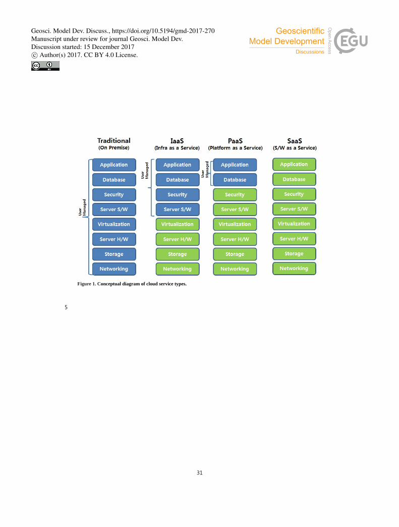
flexibly charged by usage time and resources. Depending on the type of resource provided, it is possible to

distinguish among Infrastructure as a Service (IaaS), Platform as a Service (PaaS), and Software as a Service 20

(SaaS) (Figure 1). Because cloud computing services are provided through the internet, it is possible to use various

cloud computing services if internet access is possible. Cloud computing can be categorised as public or private

depending on the deployment model (Mell and Grance, 2011). IT companies such as Amazon, Microsoft, and

IBM provide public cloud services (AWS, Azure, and Bluemix, respectively) commercially. A private cloud is

deployed by a company for internal users and purposes. In this study, we used AWS, a public cloud service that 25

can be used with IaaS option for running a numerical ocean model. Virtualisation is a key technology required to

provide services such as IaaS. Through virtualisation, physical servers, storages, and N/W resources can be

logically segmented and allocated to users, and logically returned when jobs are completed.

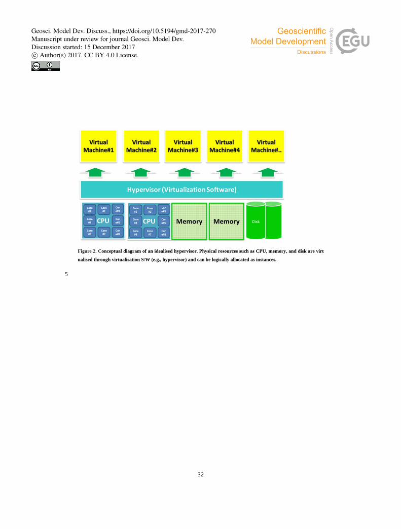
Figure 2 shows the hypervisor, a server virtualisation technology that can divide server resources logically. A

physical x86 server can be logically separated and assigned as a Virtual Machine (VM) through the hypervisor 30

(cloudacademy, 2015). The virtual servers in public cloud computing are examples of the utilisation of these

hypervisor technologies. The AWS servers used in this study are also VMs provided through this virtualisation

technology. As the VMs can be copied and stacked in the repository in the form of images, it is possible to recreate

the VMs of the same configurations by additionally creating another copy using the VM image. These techniques

provide a useful method to prepare a number of nodes, which is necessary for large-scale numerical model 35


5

experiments. It is helpful to researchers who need to setup highly complicated environments for numerical

modelling.

2.2. Commercial cloud computing services

Users of public cloud services have increased rapidly for economic or technical reasons. Major commercial public

cloud services in the global market include Amazon's AWS, Microsoft's Azure, IBM's Bluemix, and Google's 5

compute cloud service. The most popular public cloud computing service in the market is Amazon's AWS, which

has numerous datacentres and provides many services in various countries. In this study, we constructed and ran

the environment for the ocean numerical model on AWS. AWS provides PaaS and SaaS, as well as server resources,

according to the user's purpose. In addition, an increasing number of earth science organisations such as NASA

use AWS to store and process earth-related information (Chen et al., 2017). We selected the high-performance 10

VM servers with high-speed N/W to make the cluster configurations and optimise inter-server communication,

and also parallelised the ocean numerical model using them. AWS supplied us with suitable IT resources to achieve

our goal.

Table 1 (as of March 2017) gives an example of the various server resources provided by AWS (AWS, 2017c). As

the performance and functions are separated according to server instance, it is possible to combine the required 15

instances according to the purpose of the research. GPU-equipped instances, which are widely used for deep

learning and high-speed processing of images, are also available. Expensive IT resources can be used at a

reasonable price according to the usage amount. AWS’s prices vary according to datacentre. The most economic

server can be selected regardless of the distance between user and server. The datacentre and services in Oregon,

USA were selected for this study. It is also possible to use IT resources at a much lower cost by using spot-instance 20

type resources instead of on-demand type.

High-speed processor, large memory size, and high N/W throughput are essential for large-scale modelling. In

this study, we chose the recent c4-type and r4-type instances with AWS 64-bit Linux for our numerical modelling

experiment (AWS, 2017a). The c4 and r4 type instances are appropriate for numerical models that use MPI,

because AWS provides them with high bandwidth of 10 G (r4 type, 20 G) and low N/W latency. Whereas setting 25

up the environment for large-scale models in local HPC is time-consuming, setting up using c4 or r4 instances is

not. Copying several VMs for model execution reduces the time required for large-scale modelling experiments.

We were able to simulate ROMS for 30 days using eight nodes (c4.8xlarge) for only approximately US$13.

3. Numerical Model 30

3.1. High Performance Linpack Benchmarking

HPL, an implementation of Linpack Benchmarking, is a useful tool for evaluating the performance of High

Performance Computer Clusters (HPCC) (Rajan et al., 2012). It is a benchmarking software package that solves


6

a random dense linear system in double precision (64 bit) arithmetic on distributed-memory computers such as

MPI clusters. Implementation of the Basic Linear Algebra Subprogram (BLAS) is necessary for its operation.

HPL evaluates the general performance of both cloud clusters and local clusters, thereby enabling us to estimate

the effect of network and configurations of clusters before performing numerical ocean modelling. The value of

N governing complexity of tasks varies from 56000 to 125312 according to the number of processors. The 5

evaluation result of the cluster performance was calculated as FLoating Point operations per second (Flops).

3.2. Numerical Ocean Model

ROMS, which is the numerical model used in this study, is a free-surface ocean model with vertically terrain-

following and horizontally curvilinear coordinates and solves hydrostatic, free-surface primitive equations

(Shchepetkin and McWilliams, 2005). A third-order upstream advection scheme and the K-Profile 10

Parameterisation scheme (Large et al., 1994) are used for horizontal advection and vertical mixing, respectively.

Many ocean scientists use ROMS in a variety of ways to meet their research needs. ROMS comprises very modern

and modular code written in F90/F95 and uses C-pre-processing to activate the various physical and numerical

options. It has a generic distributed-memory interface that facilitates the use of several message passage protocols.

Currently, data exchange among nodes is achieved with MPI. However, other protocols such as MPI2 and 15

SHMEM can be used without much effort. Further, the entire input and output data structure of the model is via

NetCDF (ROMS, 2015).

The model domain used in this study extends from 115°E to 162°E and from 15°N to 52°N, which includes the

Yellow Sea, the East China Sea, and the East/Japan Sea (Figure 3). It features 1/10° horizontal grid resolution and

40 vertical layers. The bottom topography data is based on the Earth Topography five-minute grid (ETOPO5) 20

dataset of the National Geophysical Data Center (Amante and Eakins, 2009). The initial temperature and salinity

were obtained from the National Ocean Data Center (NODC) World Ocean Atlas 2009 (WOA09) (Antonov et al.,

2009; Locarnini et al., 2009). For the lateral open boundary, the monthly mean temperature, salinity, and velocity

from the Simple Ocean Data Assimilation (SODA; Carton and Giese, 2008) for 2010 were applied. The surface

forcing, which includes daily mean wind, solar radiation, air temperature, sea level pressure, precipitation, and 25

relative humidity, was derived from the ERA-Interim reanalysis data of the European Centre for Medium-Range

Weather Forecasts for 2010 (Dee et al., 2011). These data were applied to calculate the surface heat flux with the

bulk formulae (Fairall et al., 1996). Tidal forcing of 10 tidal components was provided by TPXO7 (Egbert and

Erofeeva, 2002). Freshwater discharges from 12 rivers were also applied in the model (Vörösmarty et al., 1996;

Wang et al., 2008). Details on the model area are given in Seo et al. (2014). 30

4. Deployment of the Numerical Ocean Model and the HPL package on AWS and the Laboratory Cluster

The same numerical experiments were conducted in the laboratory HPC environment and on AWS to compare the

performance of both environments. The laboratory HPC cluster comprises a three-node cluster consisting of Intel


7

Xeon 2 CPUs (2.6 GHz, 28 cores) per node. The HPC cluster configured in AWS was an eight-node cluster

composed of c4.8xlarge instances. The server instance provided by AWS has virtualised CPU with hyperthreads

mode enabled instead of a physical CPU. The optimal number of vCPUs per node with this configuration had to

be determined first, and then the optimal number of vCPUs extended for model performance. This is because the

performance of virtual CPUs with hyperthreads mode enabled may differ from the performance of physical servers 5

with only physical CPU.

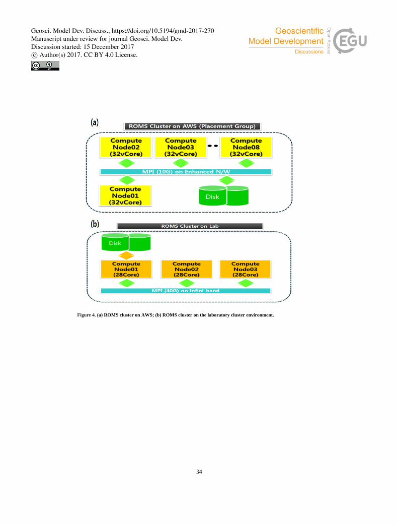
A high-speed N/W environment configuration for MPI-based parallel processing is necessary. The laboratory HPC

environment is configured as an InfiniBand high-speed network capable of achieving a maximum bandwidth of

40 Gbps with very low latency. AWS HPC can be configured as an environment supporting an Ethernet-based

high-speed network having a bandwidth of up to 20 Gbps with low latency (Table 1). In order to secure a 10

bandwidth of 10 Gbps or more and minimise latency, a separate placement group should be constructed and

configured with Virtual Private Cloud (VPC) in AWS (AWS, 2016a). A placement group is a logical grouping of

instances within a single availability zone (AWS, 2016b). Only in the same placement group is Elastic Network

Adaptor (ENA) possible (AWS, 2016c), and so the placement group labelled ‘MPI_(10G)_on_Enhanced_NW’ in

Figure 4 was constructed. A VPC, labelled ‘ROMS Cluster on AWS’ was constructed in the us-west-2 region 15

(Oregon region) and the connection between nodes made with a private Internet Protocol (IP) address. The parallel

application Open-MPI was configured and NetCDF installed for the input and output data structure of the model.

A compilation environment is optimised for cloud computing with both PGI compiler 16 and GFortran, which is

an open source compiler (Table 2).

Server resources were virtualised and deployed in AWS. Virtualised IT resources are easier to allocate and manage 20

than physical resources, but performance is slower because physical resources are provided through the software

layer. Because the N/W resources are provided via virtualisation, the network is slower than the physical N/W

environment. The technology applied to improve the speed of such virtualised N/W resources is Single Root I/O

Virtualisation (SR-IOV). AWS also adapts this technology to some high-performance instances. AWS provides an

additional high-speed N/W environment called ENA to support up to 20 Gbps bandwidth in the r4 type and 25

optimised-EBS storage performance and enhanced N/W up to 10 Gbps bandwidth in the c4 type. If the amount of

communication between nodes is large or the number of nodes increases, it is possible to configure the

environment using the instance type providing these high-performance features and achieve better numerical

modelling performance.

The SR-IOV is a technical approach to device virtualisation that provides higher I/O performance and lower CPU 30

utilisation than traditional virtualised network devices. Enhanced networking provides higher bandwidth, higher

packets per second (PPS) performance, and consistently lower latencies among instances (AWS, 2016d).

Placement groups are recommended for applications that benefit from low network latency, high network

throughput, or both. An instance type that supports enhanced networking was chosen to provide the lowest latency

and the highest PPS network performance for our placement group (AWS, 2016d). Many users may be concerned 35

about the security of cloud computing. The security of the cloud computing can be improved by employing the


8

placement group and VPC functions, and configuring the connection of the nodes with private IP addresses.

5. Results

5.1 HPL benchmark simulation

Figure 5 compares the performance of the AWS cluster and the laboratory HPC cluster. It can be seen that the 5

performance of the laboratory cluster using HPL is slightly higher than that of the AWS cluster. Further, network

latency may be smaller than in the AWS cluster, because the laboratory cluster uses an InfiniBand network. The

performance of the two clusters increases linearly with the number of cores. This experimental result suggests that

there is only marginal difference in the general performance of the two cluster configurations, which enables us

to evaluate the performance of the numerical ocean model in both clusters. 10

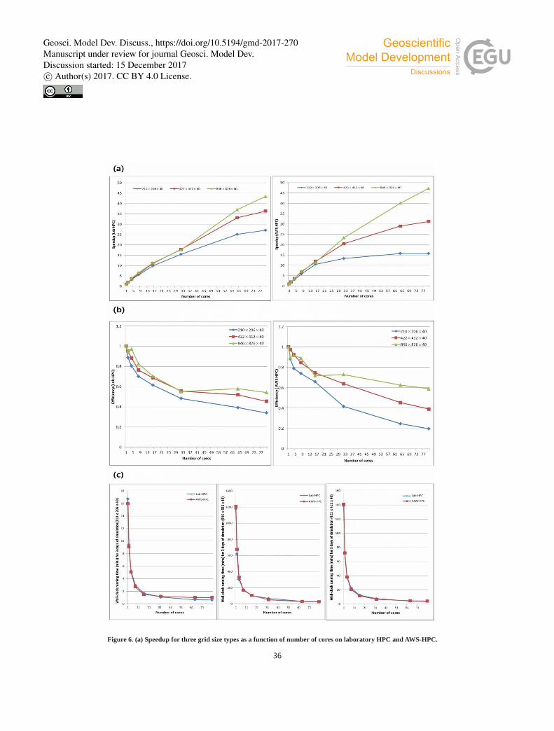
5.2 Efficiency simulation

The efficiency of the ocean model in the cluster environment was also evaluated. Figure 6 shows the speedup,

the efficiency of the ROMS, and the wall-clock running time with three different grid sizes for 3 days. We define

speedup S as follows (Pacheco, 2011):

S , 15

where Tserial is the wall-clock time of a single task job, and Tparallel is the wall-clock tine of the same work in parallel.

The efficiency E is defined as follows (Pacheco, 2011):

E ,

where S is speedup and P is the number of processor. This experimental result shows that in both clusters the

execution efficiency of the ocean model increases proportionally with the number of grids. 20

5.3 Ocean model simulation

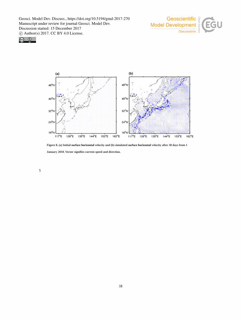
Figures 7 and 8 show the simulated Sea Surface Temperature (SST) and surface velocity initially and after 30 days

run from 1 January 2010, respectively. The Kuroshio Current, which is characterised by warm water and high

speed, is well simulated along the Okinawa trough and the eastern coast of Japan. Cold water appears in the

Okhotsk Sea, the northern East/Japan Sea, and the coast of the Yellow Sea as a result of the atmospheric cooling 25

and vertical mixing (Seo et al., 2014). Comparison of the models simulated by AWS and the local servers shows

that the Root-Mean-Square Error (RMSE) of the SST is 0.0097 ℃ and the RMSE of u-component and v-

component of the velocity is about 0.0005 ms-1. This means that the difference between the simulation results

from AWS’s HPC modelling and local HPC modelling systems is very small.


9

5.4 Comparison of HPC performance

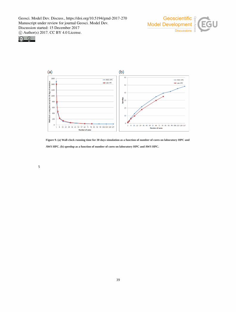
To examine speedup, groups of 16 c4.8xlarge CPUs were used to extend the AWS cluster. The CPUs were added

to the cluster (16, 32, 64, 80, 96, 112, 128 cores) in groups of 1, 2, 4, 5, 6, 7, and 8 nodes in the case of AWS. We

increased the number of processors (16, 32, 64, 80 cores) step by step in the ocean modelling test in the laboratory

HPC, in which one node has 28 physical cores. We conducted the same incremental increase using groups of 16 5

CPU units in AWS to compare performance under the same conditions.

Figure 9 shows the result of executing the ROMS in the laboratory HPC and AWS HPC environments, respectively.

The execution time for both environments followed a similar reduction pattern. However, the processing

efficiency gradually decreased. Small or medium HPC environments (100–200 cores) composed of c4.8xlarge

instance nodes in AWS have similar performance to a local HPC cluster. 10

6. Analysis of AWS instance performance

6.1 Hyperthreads effect

Many nodes are used to facilitate parallel processing in large-scale numerical models. It is necessary to consider

the number of servers and correct performance of the servers in parallel processing, because each server has more 15

cores than in the past. Allocation of the optimal vCPUs for each node and optimising the load balance of each

node to ensure enhanced performance are important in cloud computing. Hyperthreads are enabled in the CPUs

of AWS instances. However, poor knowledge of their configuration might lead to misunderstanding of a vCPU’s

performance and consideration of it as being similar to a physical CPU’s performance, which may lead to

underestimation of the AWS instance’s performance. 20

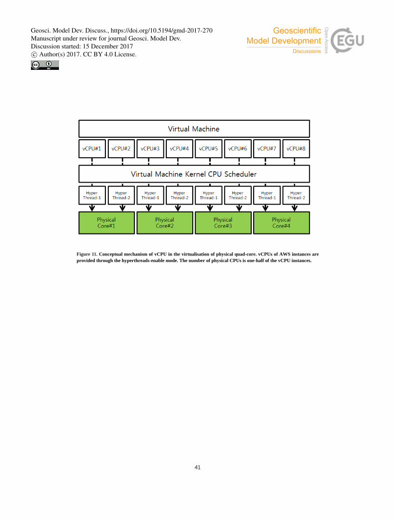
As shown in Figure 10, there is little difference in the performance of 16 cores and 32 cores. Although 32 vCPUs

are in one instance (c4.8xlarge), the actual number of physical cores is 16, because each node provided by AWS

has the hyperthreads feature enabled. If a single thread uses 100% of the resource of one physical core, the other

threads assigned to that core have to wait to use the physical resources, because the hyperthreads feature of an

Intel CPU is virtualised, as shown in Figure 11. If one CPU is used at almost 100% usage, such as a MPI job task, 25

the resource available for another thread will be insufficient. Therefore, a resource capacity plan should be

prepared based on this understanding because one node shows optimal performance at almost half of the provided

vCPUs. Two instances should be allocated to utilise 16 vCPUs per node rather than using one instance with 32

vCPUs for the performance and the output of a server with 32 physical CPUs in AWS.

6.2 S/W configurations 30

The speed of parallel processing can vary depending on the configuration and environment of the software even

in the same server environment (Chen et al., 2017). The processing time was measured under an environment with


10

PGI and GFortran compilers, which are widely used for numerical model compilation. Figure 10 shows the

performance comparison between the PGI and GFortran compilers according to the number of vCPUs. As there

is negligible difference in performance between the two compilers, PGI compiler 16, which has a commercial

version and a community version, was deployed in the following experiments.

6.3 Instance type and numbers 5

Several types of instances can be used according to research purposes. Two or three instance types were optimised

to support computation performance, memory size, and high-speed N/W. We compared the processing

performance by selecting the c4 and r4 instance types with enhanced N/W support features. The difference in

processing performance according to instance type under the same S/W environment is negligible. It is essential

to select an instance type that is optimised in advance before driving a large-scale numerical model. The instance 10

type which is optimised for numerical modelling is the c4-type instance, which is composed of the highest

computation processing CPU (Intel Xeon, 2.9 GHz). Its performance is better by approximately 5% than the r4

type (Intel Xeon, 2.3 GHz). In a cluster environment consisting of multiple nodes, the modelling performance is

similar because the amount of communication between the nodes increases with the number of nodes. The C4

type is suitable for simulating small-scale numerical models for better CPU performance. However, the difference 15

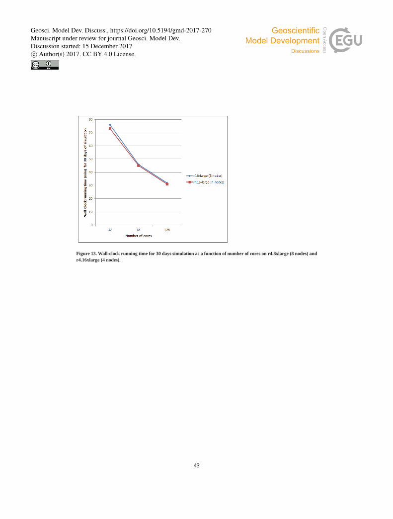
in the simulation among four or more nodes is negligible because of inter-node communication. Figure 12

compares c4-type and r4-type instances as a function of number of cores. Figure 13 shows that the difference

between r4.8xlarge (8 nodes) and r4.16xlarge (4 nodes) is negligible. This result shows that between four and

eight the number of nodes does not affect the performance of ROMS.

20

7. Conclusion

In this study, we investigated the feasibility in terms of parallel processing performance of an MPI-based ocean

modelling system (ROMS) in a commercial cloud environment. To evaluate performance more objectively,

ROMS and HPL were both executed in a laboratory HPC environment and on AWS and their performance

compared. A cluster comprising 128 cores in AWS was found to provide similar performance to the InfiniBand 25

environment cluster in ocean modelling. AWS is a useful infrastructure for numerical ocean models such as ROMS,

which is a low N/W latency sensitive model. Two instance types and parallel processing with MPI in AWS were

tested to measure the performance of the numerical model. Further, two compilers with community versions were

used to examine the S/W environment effects. The performance pattern in AWS was found to be similar to that in

the laboratory HPC for both c4 and r4 instance types, irrespective of the number of nodes. 30

The performance of cloud computing environments is constantly improving, and various numerical models are

being tested in cloud computing environments. Microsoft's Azure already supports InfiniBand N/W technology

and N/W sensitive models can be tested in InfiniBand-supported cloud environments easily in the near future.

Some models may depend on the size of the memory according to the grid size and the communication latency


11

between the nodes as well as the computation. These constraints can be satisfied by suitable selection and

operation of instance types in cloud computing environments such as AWS. This study shows how numerical

ocean models can be constructed and parallelised in a commercial cloud computing environment. It also outlines

how performance similar to local HPC can be achieved in commercial cloud computing environments by

optimising the modelling environment. The commercial cloud computing environment is a cost-effective solution 5

for large-scale modelling. Various technologies are available for enhancing the security of cloud computing to the

level of that of local HPC. Moreover, node image replication techniques such as Amazon Machine Image (AMI)

(AWS, 2017b) can be used to copy the model environment configuration of the ocean numerical model rapidly in

commercial cloud environments, making it easy to expand, transfer, duplicate, and change nodes. This makes it

easier to collaborate among researchers in a multinational context. Thus, cloud computing provides the 10

opportunity to focus on research and to minimise the amount of resource commitment needed to construct a

modelling environment.


12

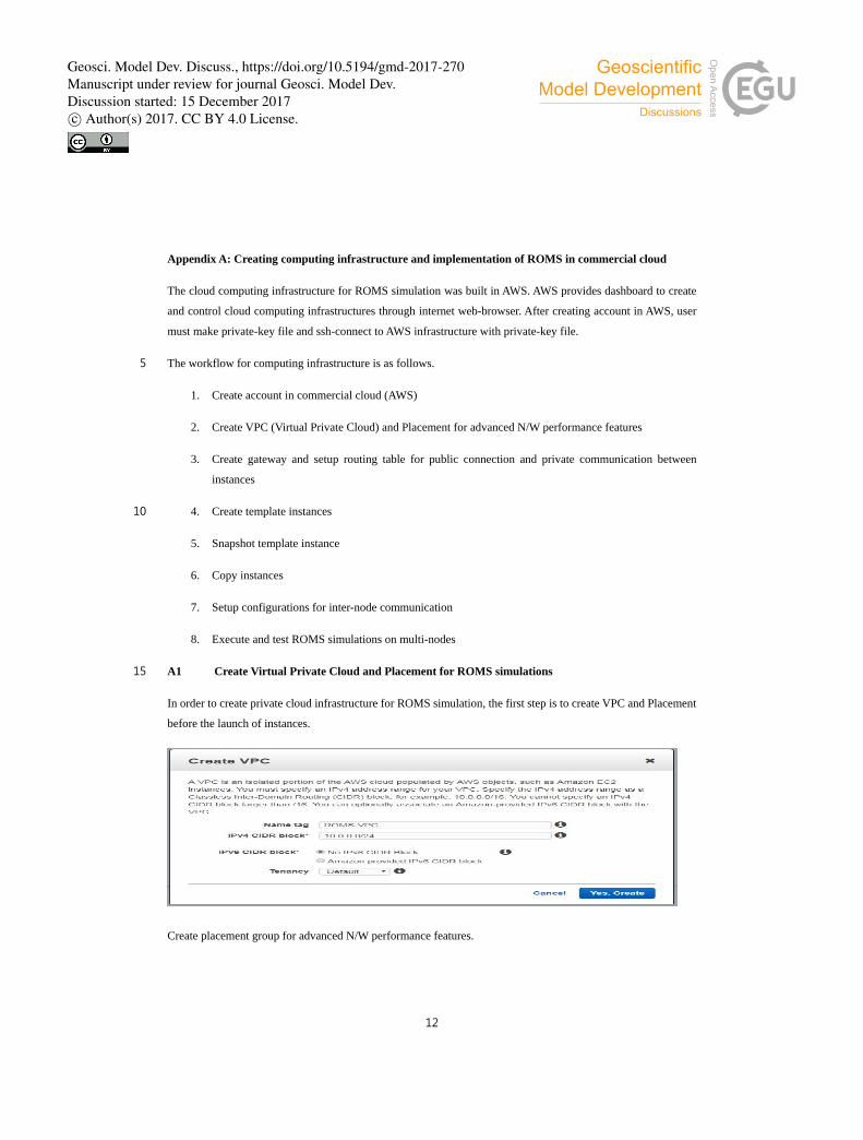
Appendix A: Creating computing infrastructure and implementation of ROMS in commercial cloud

The cloud computing infrastructure for ROMS simulation was built in AWS. AWS provides dashboard to create

and control cloud computing infrastructures through internet web-browser. After creating account in AWS, user

must make private-key file and ssh-connect to AWS infrastructure with private-key file.

The workflow for computing infrastructure is as follows. 5

1. Create account in commercial cloud (AWS)

2. Create VPC (Virtual Private Cloud) and Placement for advanced N/W performance features

3. Create gateway and setup routing table for public connection and private communication between

instances

4. Create template instances 10

5. Snapshot template instance

6. Copy instances

7. Setup configurations for inter-node communication

8. Execute and test ROMS simulations on multi-nodes

A1 Create Virtual Private Cloud and Placement for ROMS simulations 15

In order to create private cloud infrastructure for ROMS simulation, the first step is to create VPC and Placement

before the launch of instances.

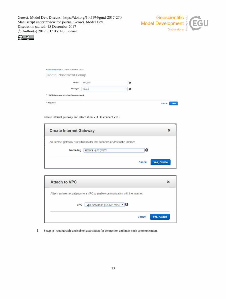
Create placement group for advanced N/W performance features.


13

Create internet gateway and attach it on VPC to connect VPC.

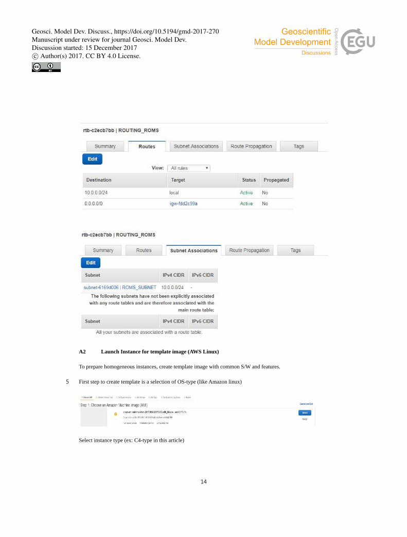
Setup ip- routing table and subnet association for connection and inter-node communication. 5


14

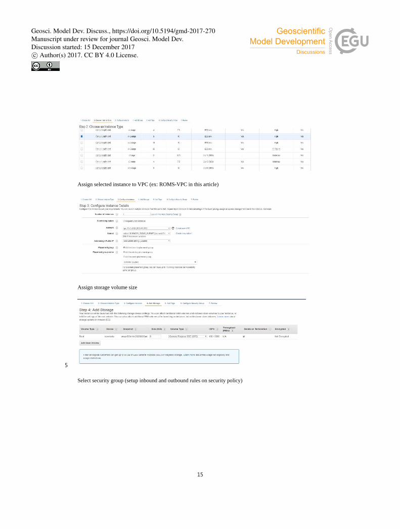
A2 Launch Instance for template image (AWS Linux)

To prepare homogeneous instances, create template image with common S/W and features.

First step to create template is a selection of OS-type (like Amazon linux) 5

Select instance type (ex: C4-type in this article)


15

Assign selected instance to VPC (ex: ROMS-VPC in this article)

Assign storage volume size

5

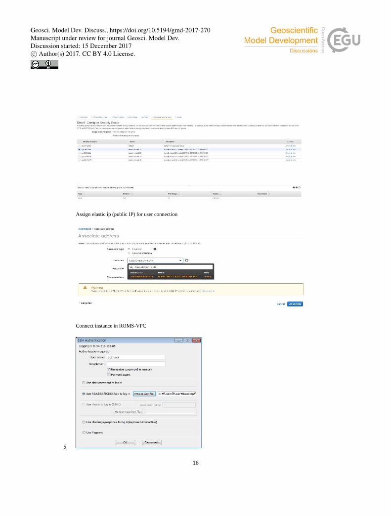
Select security group (setup inbound and outbound rules on security policy)


16

Assign elastic ip (public IP) for user connection

Connect instance in ROMS-VPC

5


17

AWS default account is ec2-user with private-key file

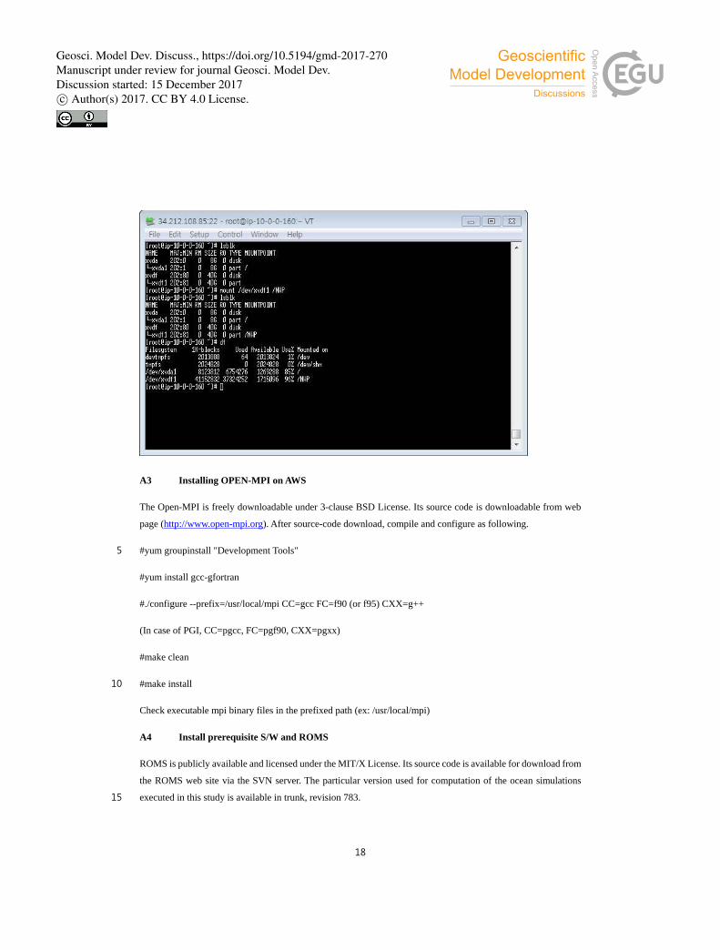
Attach additional file-system for simulations (Optional)

#lsblk 5

#mount /dev/xvdf /NWP (ex: /NWP in this article)


18

A3 Installing OPEN-MPI on AWS

The Open-MPI is freely downloadable under 3-clause BSD License. Its source code is downloadable from web

page (http://www.open-mpi.org). After source-code download, compile and configure as following.

#yum groupinstall "Development Tools" 5

#yum install gcc-gfortran

#./configure --prefix=/usr/local/mpi CC=gcc FC=f90 (or f95) CXX=g++

(In case of PGI, CC=pgcc, FC=pgf90, CXX=pgxx)

#make clean

#make install 10

Check executable mpi binary files in the prefixed path (ex: /usr/local/mpi)

A4 Install prerequisite S/W and ROMS

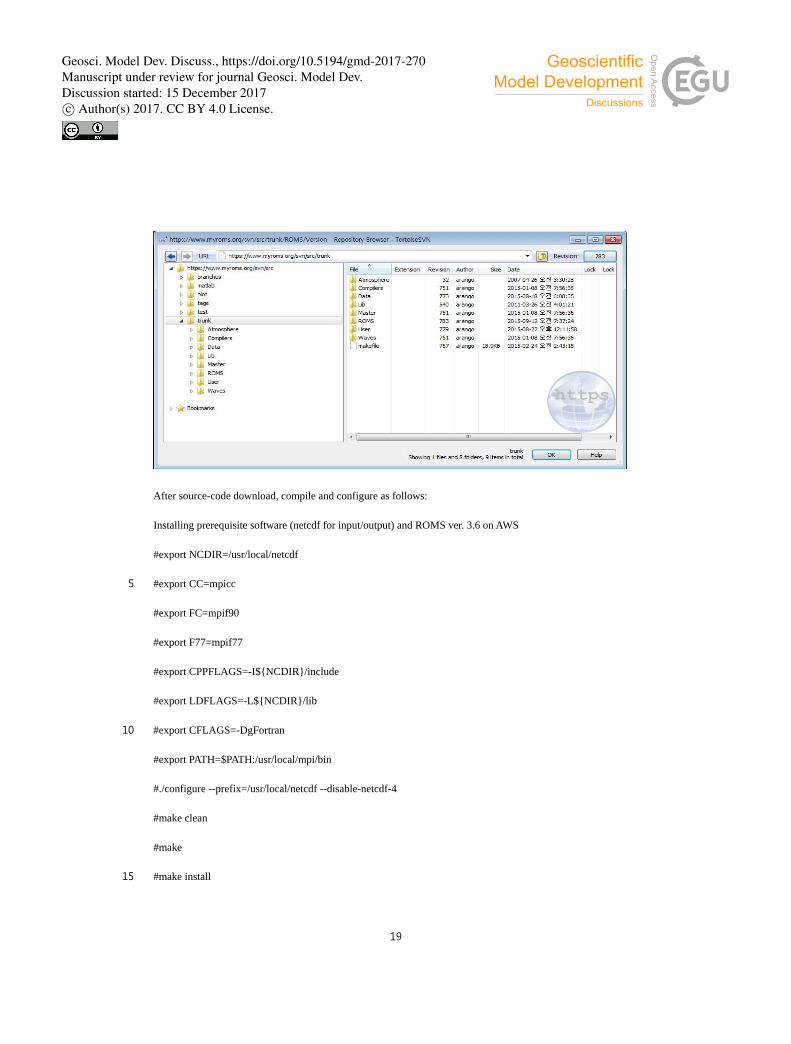
ROMS is publicly available and licensed under the MIT/X License. Its source code is available for download from

the ROMS web site via the SVN server. The particular version used for computation of the ocean simulations

executed in this study is available in trunk, revision 783. 15


19

After source-code download, compile and configure as follows:

Installing prerequisite software (netcdf for input/output) and ROMS ver. 3.6 on AWS

#export NCDIR=/usr/local/netcdf

#export CC=mpicc 5

#export FC=mpif90

#export F77=mpif77

#export CPPFLAGS=-I${NCDIR}/include

#export LDFLAGS=-L${NCDIR}/lib

#export CFLAGS=-DgFortran 10

#export PATH=$PATH:/usr/local/mpi/bin

#./configure --prefix=/usr/local/netcdf --disable-netcdf-4

#make clean

#make

#make install 15


20

Before compiling ROMS source codes, add PATH and LD_LIBRARAY_PATH in profile.

#export LD_LIBRARY_PATH=/lib64:/usr/lib:/usr/local/lib:/usr/lib64:/usr/local/mpi/lib:/usr/local/netcdf/lib

#export PATH=$PATH: /usr/local/mpi/bin

Edit specific compiler.mk according to compiler type.

5

Add FC field and NECDF according to specific environment (ex: gfortran and /usr/local/netcdf).


21

Set ROMS/TOMS executable file name.

#--------------------------------------------------------------------------

ifdef USE_MPI

BIN := $(BINDIR)/aws_roms_test_gfort (aws_roms_test_gfort in this example)

Endif 5

#---------------------------------------------------------------------------

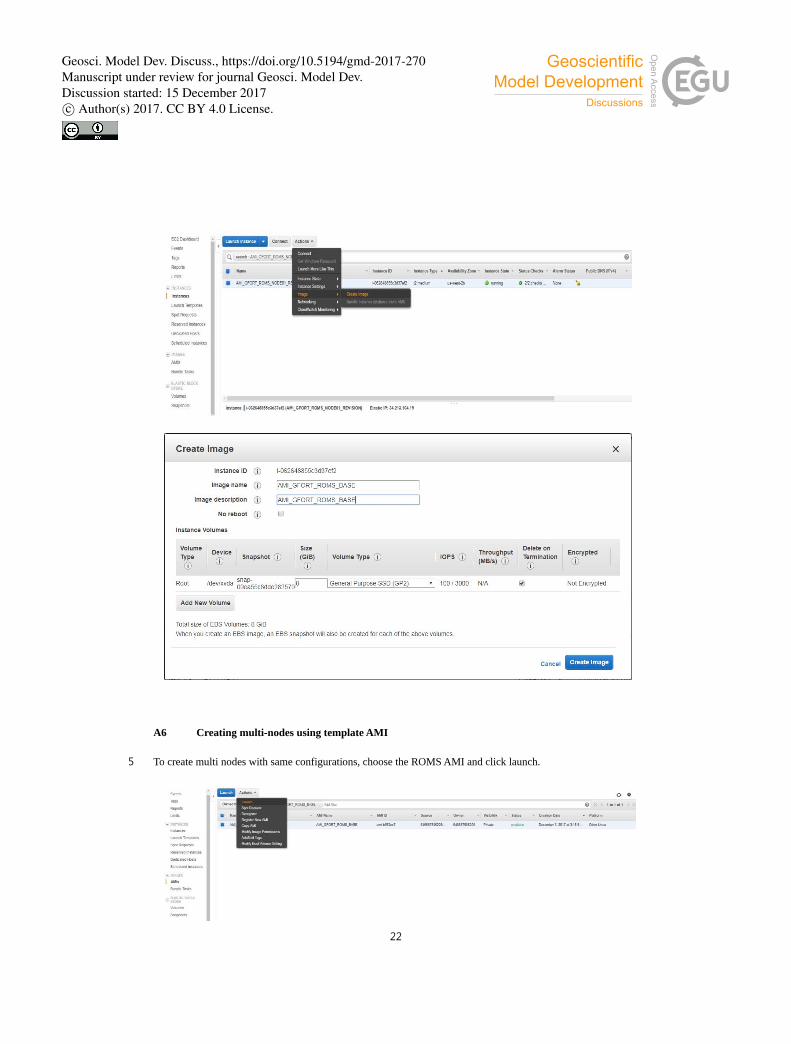
A5 Create AMI (Amazon Machine Image)

After completion of template configurations, create ROMS AMI to make multi-nodes with little effort. In AWS, 10

private AMI is also shareable under private permission. Including AWS, commercial cloud companies provide

tools to create template images.

Creating AMI (Amazon Machine Image) from template instance


22

A6 Creating multi-nodes using template AMI

To create multi nodes with same configurations, choose the ROMS AMI and click launch. 5


23

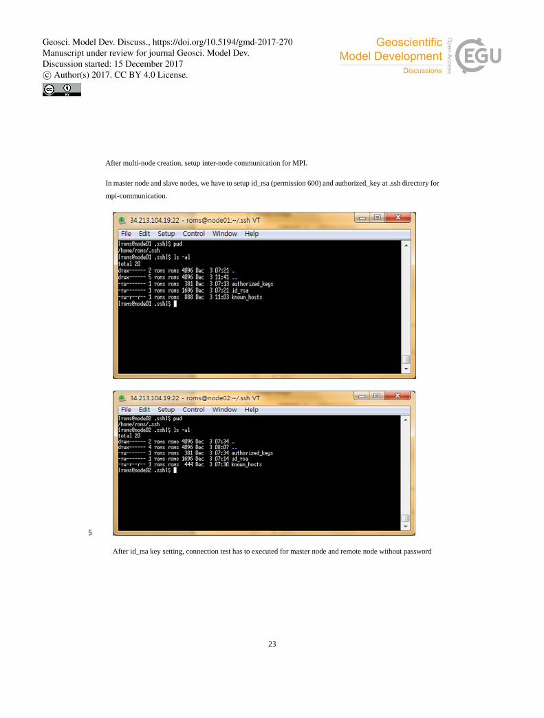
After multi-node creation, setup inter-node communication for MPI.

In master node and slave nodes, we have to setup id_rsa (permission 600) and authorized_key at .ssh directory for

mpi-communication.

5

After id_rsa key setting, connection test has to executed for master node and remote node without password


24

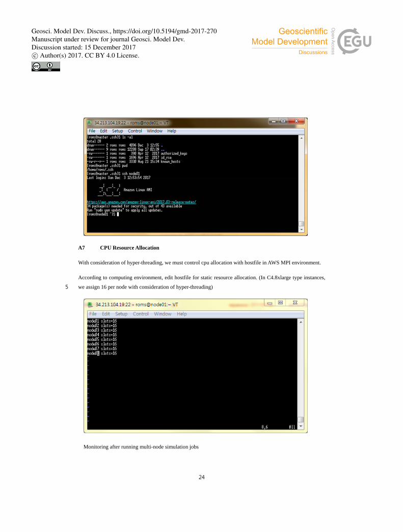
A7 CPU Resource Allocation

With consideration of hyper-threading, we must control cpu allocation with hostfile in AWS MPI environment.

According to computing environment, edit hostfile for static resource allocation. (In C4.8xlarge type instances,

we assign 16 per node with consideration of hyper-threading) 5

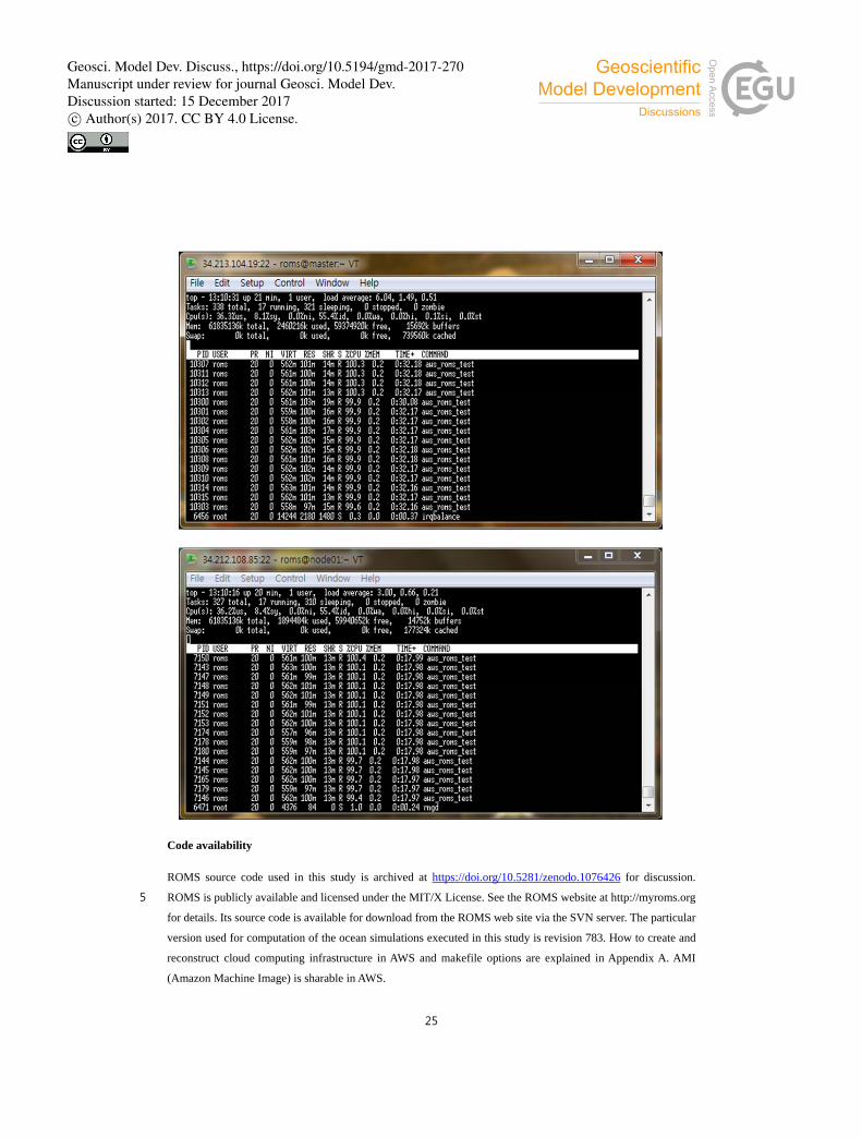
Monitoring after running multi-node simulation jobs


25

Code availability

ROMS source code used in this study is archived at https://doi.org/10.5281/zenodo.1076426 for discussion.

ROMS is publicly available and licensed under the MIT/X License. See the ROMS website at http://myroms.org 5

for details. Its source code is available for download from the ROMS web site via the SVN server. The particular

version used for computation of the ocean simulations executed in this study is revision 783. How to create and

reconstruct cloud computing infrastructure in AWS and makefile options are explained in Appendix A. AMI

(Amazon Machine Image) is sharable in AWS.


26

Author contributions

All authors participated into the design of the experiments and analysis of the results. Kwangwoog Jung

implemented the full infrastructure for the experiments. Yang-Ki Cho analysed the results from AWS HPC and

laboratory HPC. Yong-Jin Tak carried out the laboratory HPC benchmarking tests. All authors participated in the

writing of this paper. 5

Competing interests

The authors declare that they have no conflicts of interest.

Acknowledgement

Y.-K. Cho was supported by the ‘Walleye Pollock Stock Management based on Marine Information & 10 Communication Technology’ project, funded by the Ministry of Oceans and Fisheries, Korea.


27

References

Amante, C. and Eakins, B. W.: ETOP01 1 arc-minute global relief model: Procedures, data sources and analysis, NOAA Tech. Memo., NESDIS NGDC-24, p. 19, 2008.

Antonov, J. I., Seidov, D., Boyer, T. P., Locarnini, R. A., Mishonov, A. V., Garcia, H. E., Baranova, O. K., Zweng, M. M., and Johnson, D. R.: World Ocean Atlas 2009, Volume 2: Salinity. S. Levitus, Ed. NOAA Atlas NESDIS 5 69, U.S. Government Printing Office, Washington, D.C., p. 184, 2010

AWS: Virtual Private Cloud, available at: https://aws.amazon.com/vpc/?nc1=h_ls/ (last accessed: 09 May 2017), 2016a.

AWS: Placement Groups, available at: http://docs.aws.amazon.com/AWSEC2/latest/WindowsGuide/placement-groups.html (last accessed: 09 May 2017), 2016b. 10

AWS: Elastic Network Adaptor, available at: https://aws.amazon.com/ko/about-aws/whats-new/2016/06/introducing-elastic-network-adapter-ena-the-next-generation-network-interface-for-ec2-instances/ (last accessed: 03 March 2017), 2016c.

AWS: Enhanced Networking, available at: http://docs.aws.amazon.com/AWSEC2/latest/UserGuide/enhanced-networking.html (last accessed: 03 April 2017), 2016d 15

AWS: Amazon Linux, available at: https://aws.amazon.com/amazon-linux-ami/?nc1=h_ls (last accessed: 03 March 2017), 2017a.

AWS: Amazon Machine Images, available at: http://docs.aws.amazon.com/AWSEC2/latest/UserGuide/AMIs.html (last accessed: 03 March 2017), 2017b.

AWS: AWS Pricing, available at: https://aws.amazon.com/ec2/pricing/on-demand/?nc1=h_ls (last accessed: 03 20 March 2017), 2017c.

Carton, J. A., and Giese, B. S.: A reanalysis of ocean climate using Simple Ocean Data Assimilation (SODA), Mon. Weather Rev., 136, 2999–3017, 2008.

Chen, X., Huang, X., Jiao, C., Flanner, M., Raeker, T., and Palen, B.: Running climate model on a commercial cloud computing environment: A case study using Community Earth System Model (CESM) on Amazon AWS, 25 Computers & Geo., 98, 21-25, doi: http://dx.doi.org/10.1016/j.cageo.2016.09.014. , 2017.

Cloudacademy: Xen Hypervisor, available at: https://cloudacademy.com/blog/aws-ami-hvm-vs-pv-paravirtual-amazon last accessed: 05 March 2017, 2015.

Dee, D. P., Uppala, S. M., Simmons, A. J., Berrisford, P., Poli, P., Kobayashi, S., Andrae, U., Balmaseda, M. A., Balsamo, G., Bauer, P., Bechtold, P., Beljaars, A. C. M., van de Berg, L., Bidlot, J., Bormann, N., Delsol, C., 30 Dragani, R., Fuentes, M., Geer, A. J., Haimberger, L., Healy, S. B., Hersbach, H., Hólm, E. V., Isaksen, L., Kållberg, P., Köhler, M., Matricardi, M., McNally, A. P., Monge-Sanz, B. M., Morcrette, J. –J., Park, B. –K., Peubey, C., de Rosnay, P., Tavolato, C., Thépaut, J.-N., and Vitart, F.: The ERA-Interim reanalysis: Configuration and performance of the data assimilation system, Q. J. R. Meteorol. Soc., 137(656), 553–597, doi:10.1002/qj.828, 2011. 35

Egbert, G. D., and Erofeeva, S. Y.: Efficient inverse modeling of Barotropic Ocean Tides, J. Atmos. Oceanic Technol., 19, 183–204, doi:http://dx.doi.org/10.1175/1520-0426(2002)019<0183:EIMOBO>2.0.CO;2,2002.


28

Fairall, C. W., Bradley, E. F., Rogers, D. P., Edson, J. B., and Young, G. S.: Bulk parameterization of air–sea fluxes for Tropical Ocean–Global Atmosphere Coupled–Ocean Atmosphere Response Experiment, J. Geophys. Res., 101(C2), 3747–3764, doi:10.1029/95JC03205,1996.

Large, W. G., McWilliams, J. C., and Doney, S. C.: Oceanic vertical mixing: A review and a model with a nonlocal boundary layer parameterization, Rev. Geophys., 32, 363–403, doi:10.1029/94RG01872,1994. 5

Locarnini, R. A., Mishonov, A. V., Antonov, J. I., Boyer, T. P., Garcia, H. E., Baranova, O. K., Zweng, M. M., and Johnson, D. R.: World Ocean Atlas 2009, Volume 1: Temperature. S. Levitus, Ed. NOAA Atlas NESDIS 68, U.S. Government Printing Office, Washington, D.C., p. 184, 2010.

Mell, P. and Grance, T.: The NIST definition of cloud computing recommendations of the National Institute of Standards and Technology, Special Publication 800–145, NIST, Gaithersburg, available at: 10 http://nvlpubs.nist.gov/nistpubs/Legacy/SP/nistspecialpublication800-145.pdf (last accessed: 10 March 2017), 2011.

Microsoft: Azure support for Linux RDMA, available at https://azure.microsoft.com/en-us/updates/azure-support-for-linux-rdma (last accessed: 03 March 2017), 2015.

Montes, D., Añel, J. A., Pena, T. F., Uhe, P., and Wallom, D. C. H.: Enabling BOINC in infrastructure as a service 15 cloud system, Geosci. Model Dev., 10, 811-826, doi: 10.5194/gmd-10-811-2017., 2017.

Oesterle, F., Ostermann, S., Prodan, R., and Mayr, G.J.: Experiences with distributed computing for meteorological applications: Grid computing and cloud computing, Geosci. Model Dev., 8, 2067-2078, doi: 10.5194/gmd-8-2067-2015., 2015.

Pacheco, P.: An Introduction to Parallel Programming, Morgan Kaufmann Publisher Inc., Burlington, MA, USA, 20 2011.

PGI: Community Edition, available at: http://www.pgroup.com/products/community.htm (last accessed: 03 March 2017), 2016.

Rajan, A., Joshi, B. K., Rawat, A., Jha, R., and Bhachavat, K.: Analysis of process distribution in HPC cluster using HPL: 2nd IEEE International Conference on Parallel, Distributed and Grid Computing, Solan, India, 85-88, 25 doi:10.1109/PDGC.2012.6449796, 2012.

ROMS: Regional Ocean Modeling System (ROMS), available at: https://www.myroms.org/ (last accessed: 09 May 2017), 2015.

Seo, G. -H., Cho, Y. –K., Cho, B. –J., Kim, K. –Y., Kim, B. –g., and Tak, Y. -J.: Climate change projection in the Northwest Pacific marginal seas through dynamic downscaling, J. Geophys. Res., 119, 3497–3516, 30 doi:10.1002/2013JC009646, 2014.

Shchepetkin, A. F. and McWilliams, J. C.: The Regional Oceanic Modeling System (ROMS): A split-explicit, free-surface, topography-following-coordinate oceanic model, Ocean Modell., 9, 347–404, doi: 10.1016/j.ocemod.2004.08.002, 2005.

Vörösmarty, C., Fekete, B., and Tucker, B.: River discharge database version 1.0 (RivDIS v1.0), Vol. 0–6., A 35 contribution to IHP-V theme 1, 1996.

Wang, Q., Guo, X., and Takeoka, H.: Seasonal variations of the Yellow River plume in the Bohai Sea: A model study, J. Geophys. Res., 113, C08046, doi: 10.1029/2007JC004555, 2008.


29

Table 1 Overview of the purpose, specifications, and price of AWS instance types (us-west-2, Oregon)

Type Purpose Sub-Type CPU Memory (GB) N/W Price/h

T

t2.small

t2.medium

t2.large

t2.xlarge

t2.2xlarge

1

2

2

4

8

2.0

4.0

8.0

16.0

32.0

Low/Moderate

Low/Moderate

Low/Moderate

Low/Moderate

Low/Moderate

0.023

0.047

0.094

0.188

0.376

M General purpose

instances

m4.large

m4.xlarge

m4.2xlarge

m4.4xlarge

m4.10xlarge

m4.16xlarge

2

4

8

16

40

64

8.0

16.0

32.0

64.0

160.0

256.0

Moderate

High

High

High

10G

10G

0.108

0.215

0.431

0.862

2.155

3.447

C

Compute-

optimised

instances

c4.large

c4.xlarge

c4.2xlarge

c4.4xlarge

c4.8xlarge

2

4

8

16

36

3.7

7.5

15.0

30.0

60.0

Moderate

Moderate

High

High

10G

0.100

0.199

0.398

0.796

1.591

R

memory-

intensive

applications

r4.large

r4.xlarge

r4.2xlarge

r4.4xlarge

r4.8xlarge

r4.16xlarge

2

4

8

16

32

64

15.2

30.5

61.0

122.0

244.0

488.0

Moderate

Moderate

High

10G

10G

20G

0.133

0.266

0.532

1.064

2.128

4.256

P GPU instance

p2.xlarge

p2.8xlarge

p2.16xlarge

4

32

64

61

488

732

10G

20G

0.9

7.2

14.4


30

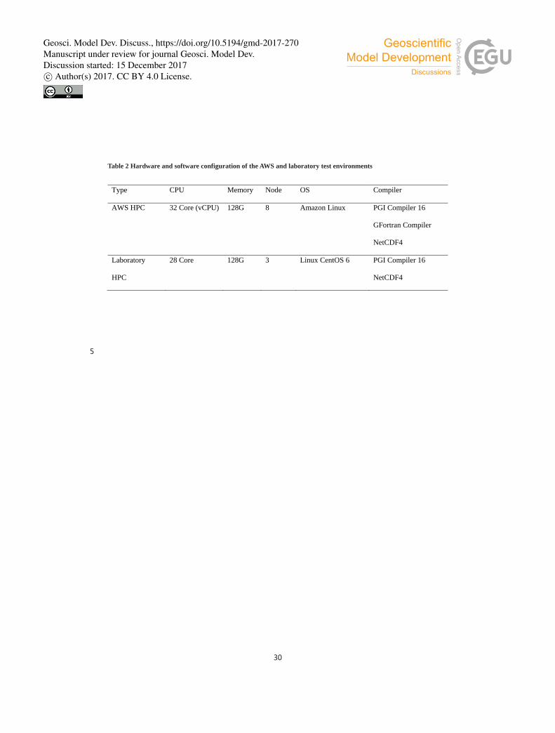
Table 2 Hardware and software configuration of the AWS and laboratory test environments

Type CPU Memory Node OS Compiler

AWS HPC 32 Core (vCPU) 128G 8 Amazon Linux PGI Compiler 16

GFortran Compiler

NetCDF4

Laboratory

HPC

28 Core 128G 3 Linux CentOS 6 PGI Compiler 16

NetCDF4

5


31

Figure 1. Conceptual diagram of cloud service types.

5


32

Figure 2. Conceptual diagram of an idealised hypervisor. Physical resources such as CPU, memory, and disk are virt

ualised through virtualisation S/W (e.g., hypervisor) and can be logically allocated as instances.

5


33

Figure 3. The domain of this study. The model domain covers 15-52˚N and 115-162˚E, which includes the East China

Sea, Yellow Sea, East Sea, and the north-western part of the Pacific. Colour signifies water depth.


34

Figure 4. (a) ROMS cluster on AWS; (b) ROMS cluster on the laboratory cluster environment.


35

Figure 5. Performance of the two clusters as a function of number of cores using the HPL S/W package.


36

Figure 6. (a) Speedup for three grid size types as a function of number of cores on laboratory HPC and AWS-HPC.


37

(b) Efficiency for three grid-size types as a function of number of cores on laboratory HPC and AWS-HPC. (c) Wall-

clock running time for three grid-size types as a function of number of cores on laboratory HPC and AWS-HPC.

Figure 7. (a) Initial sea surface temperature and (b) simulated sea surface temperature after 30 days from 1 January

2010. 5


38

Figure 8. (a) Initial surface horizontal velocity and (b) simulated surface horizontal velocity after 30 days from 1

January 2010. Vector signifies current speed and direction.

5


39

Figure 9. (a) Wall-clock running time for 30 days simulation as a function of number of cores on laboratory HPC and

AWS HPC. (b) speedup as a function of number of cores on laboratory HPC and AWS HPC.

5


40

Figure 10. (a) Wall-clock running time for 30 days simulation as a function of number of cores and compilers. (b)

Speedup for 30 days simulation as a function of number of cores and compilers.


41

Figure 11. Conceptual mechanism of vCPU in the virtualisation of physical quad-core. vCPUs of AWS instances are provided through the hyperthreads-enable mode. The number of physical CPUs is one-half of the vCPU instances.


42

Figure 12. (a) Wall-clock running time for 30 days simulation as a function of number of cores on c4-type and r4-type

instances. (b) Speedup as a function of number of cores on c4-type and r4-type instances.

5

10


43

Figure 13. Wall-clock running time for 30 days simulation as a function of number of cores on r4.8xlarge (8 nodes) and r4.16xlarge (4 nodes).


performance evaluation of roms v3.6 on a commercial cloud ...€¦ · many commercial cloud...

Documents