performance of low dissipative shock-capturing schemes … · 2013-08-30 · performance of low...
TRANSCRIPT

iii
/;<S_ 208236NASA/CR-
Research Institute for Advanced Computer ScienceNASA Ames Research Center
Performance of Low Dissipative High OrderShock-Capturing Schemes forShock-Turbulence Interactions
N.D. Sandham and H.C. Yee
RIACS Technical Report 98.10April 1998
Invited paper for the 6th ICFD Conference on Numerical Methods for Fluid Dynamics,March 31 - April 3, 1998
University of Oxford, Oxford, England
https://ntrs.nasa.gov/search.jsp?R=19980201093 2018-07-10T03:04:17+00:00Z
Performance of Low Dissipative High OrderShock-Capturing Schemes for
Shock-Turbulence Interactions
N.D. Sandham and H.C. Yee
The Research Institute for Advanced Computer Science is operated by Universities Space ResearchAssociation, The American City Building, Suite 212, Columbia, MD 21044 (410) 730-2656
Work reported herein was supported by NASA via Cooperative Agreement NCC 2-1006 betweenNASA and the Universities Space Research Association (USRA). Work performed at the ResearchInstitute for Advanced Computer Science (RIACS), NASA Ames Research Center, Moffett Field,CA 94035-1000
• ii̧
i i,_
i_ :ii̧
Performance of Low Dissipative High Order
Shock-Capturing Schemes forShock-Turbulence Interactions
N. D. Sandham*and H. C. Yee t
May 15, 1998
Abstract
Accurate and efficient direct numerical simulation of turbulence in
the presence of shock waves represents a significant challenge for nu-
merical methods. The objective of this paper is to evaluate the perfor-
mance of high order compact and non-compact central spatial differ-
encing employing total variation diminishing (TVD) shock-capturing
dissipations as characteristic :based filters for two model problems com-
bining shock wave and shear layer phenomena. A vortex pairing model
evaluates the ability of the schemes to cope with shear layer instability
and eddy shock waves, while a shock wave impingement on a spatially-
evolving mixing layer model studies the accuracy of computation of
vortices passing through a sequence of shock and expansion waves.A drastic increase in accuracy is observed if a suitable artificial com-
pression formulation is applied to the TVD dissipations. With this
modification to the filter step the fourth-order non-compact scheme
shows improved results in comparison to second-order methods, while
retaining the good shock resolution of the basic TVD scheme. For thischaracteristic based filter approach, however, the benefits of compact
schemes or schemes with higher than fourth order are not sufficient to
justify the higher complexity near the boundary and/or the additional
computational cost.
*Queen Mary and Westfield College, London, UKtNASA Ames Research Center, Moffett Field, CA, USA
.i_ _ .,

_ _i?_̧¸:_ _!_i!i!ii!i_iii_ii!_!_:,:, _i__!_!_!!__i__i i, i _!/__?ii ............../!_!ii_i_ _i,!iiiii_ii_i¸
i _ii iiiiiiii_i_i_/i_ii__
1 Introduction
Time-and space-resolved direct numerical simulation (DNS) of turbulence is
feasible for many canonical flow problems (Moin _z Mahesh, 1998) andwith
increased computer power more applied problems such as separation bubbles
(Alam _z Sandham, 1997) can also be simulated. For many technologically
important flows compressibility effects are important. Direct simulation is
already playing an important role in understanding effects such as the re-
duced growth rate of mixing layers as Mach number is increased (Vreman
et al., 1996). With high speed compressible flows, however, the potential
combination of shock waves and turbulent flow represents a significant chal-
lenge for numerical methods. Although standard total variation diminishing
(TVD) type of shock-capturing schemes for the Euler equations (Yee, 1989)are now routinely used in high speed blast wave simulations with virtually
non-oscillatory, crisp resolution of discontinuities, for the unaveraged un-
steady Navier-Stokes equations it was observed (Sandham &=Yee 1989) that
the clipping behavior near extrema of these schemes led to generally poor
accuracy.
In response to this difficulty, subsequent large three-dimensional computa-
tions have either operated at low :Reynolds and Mach numbers where the
shock waves, if present at all, are weak and can be resolved (Luo _ Sand-
ham, 1994)or have used hybrid schemes where shock-capturing schemes areturned on only when shock waves are detected (Vreman et al., 1995, Adams
&=Shariff, 1996, Adams, 1997 and Lee et hi., 1997). These calculations haveall used base methods of fourth or sixth-order accuracy, well suited to the
accurate calculation of turbulence.
Work has continued on model problems to find improved high order shock-
capturing schemes. Lumpp (1996a,b) used high order finite volume es-
sentially non-oscillatory: (ENO)schemes for vortex pairing test case.s and
obtained good shock and vortex resolution. However, large grid stencils
and high computational cost has prohibited application to three-dimensional
problems. Fu and Ma (1997) have developed a scheme where the group veloc-
ity near shock waves is fixed by the numerical method such that oscillationsnear shock waves are sucked into the shock wave itself, giving very sharp
shocks. In another development Yee (1997) has developed a class of compact
shock-capturing schemes that require smaller grid stencils and operations
count than standard schemes.Gustafssonand Olsson (1995) developedsta-ble higher-order centeredschemeswith stable numerical boundary conditiontreatments. For problems containing shocks,Gustafsson and Olsson useda scalar shock-capturing filter. Suchschemeshave advantages:overhigher-order ENO schemeswhich require very large grid stencils even for modestorders of accuracy. (For example, a seven-point grid stencil is required fora second-orderENO scheme.) Yee et al. (1998) proposed a combinationof narrow grid stencil of higher-order classicalspatial differencing schemesusing low order TVD or ENO dissipations as characteristic filters with anartificial compressionmethod (ACM) switch. The ACM switch is the sameas Harten (1978) but applied in a slightly different context. The Yeeet al.approach is aimed at problemscontaining vortex convections,shock, shear,vortex and turbulence interactions. Thesecharacteristic TVD (and ENO)fil-ters in conjunction with the artificial compressionmethod can evenimprovefine scaleflow structure when applied to existing methods of Yee (1989)andYee (1997).
A numerical schemefor DNS of shock-turbulenceinteractions should ideallynot be significantly more expensivethan the classical fourth or sixth-ordercompact or non-compactspatial differencingscheme.It shouldbe possibletoresolveall scalesdown to scalesof the order of (if necessary)the Kolmogorovscalesof turbulence accurately and efficiently, while at the sametime beingable to capture steep gradientsoccurring at smaller scales(e.g. a few meanfree paths for a strong shockwave). Turbulence mechanismsshould not beaffectedby the numerical schemeresulting directly from the governingequa-tions. Someearly direct simulation codesfor incompressibleflow wereunableto sustain turbulence in channel flow due to their properties with respect toaliasing errors. Shock-capturing schemesare dissipative and an importanttest of their suitability for turbulence is that they are capable of sustainingturbulence. The purposeof the presentwork is to evaluatea number of can-didate schemesdiscussedin Yeeet al. (1998) using model problems. In thefirst of these, a vortex pairing in a time-developingmixing layer, shockwavesform around the vortices. In the secondproblem, a shock wave impingingon a spatially-evolving mixing layer, the evolving vortices must passthrougha shockwave, which in turn is deformed by the vortex passage.From thesetwo-dimensional tests someconclusionscan be drawn regarding numericalmethods for accurate calculation of vortex motions within an overall shock-
• :j!
capturing framework.
2 i iNumer cal Techn ques
The numerical methods used for the study are briefly described in this sec-
tion. The reader is referred to Yee (1989) for a more complete description of
the basic shock-capturing approaches and Yee et al. (1998) for the complete
scheme.
The classical fourth-order Runge-Kutta time discretization and classical fourth
or sixth-order compact or non-compact spatial differencing as base schemes
are employed. A second-order TVD dissipation is applied as a filter step atthe end of the full Runge-Kutta time step in the form of an additional dissi-
pative numerical flux term
1• _ __ _ _ (1)
where R is the right eigenvector matrix of the flux J acobian from the Euler
equations and • is defined by the TVD shock-capturing scheme. The de-
tailed programming allows the Euler and viscous terms to be computed us-
ing separate methods The basic spatial schemes are (i) non-compact central,
(ii) compact central and (iii) predictor-corrector upwind or upwind biased.
Non-compact schemes are the standard second, fourth and sixth-order meth-
ods. Compact schemes are either the standard symmetric fourth,order or
sixth-order Pade schemes (Ciment & Leventhal, 1975, Hirsh, 1975 and Lele,
1992). For the purposes of this paper we concentrate on the central schemes.
Comparable accuracy was obtained with the predictor-corrector upwind or
upwind biased schemes proposed by Hixon and Turkel (1998).
TVD Dissipation as a Filter Step
The TVD dissipation as a filter step is taken as the diffusive part of an
upwind explicit shock-capturing scheme of the Harten-Yee type, described in
Yee (1989). (Other comparable schemes are also applicable.) For a second-
order upwind TVD scheme the elements of _j+½, denoted by Cj+½, are
¢_ 1 1 l l 1 ___ r-)/_.___ 1 ) OLd_{_ 1+_ -- _¢(a_+½)(g}+l + gj) - ¢(aj+_
- "_T:_iii_iiiiii!i) i!iiii< iii:L;_: qi:_ i; ¸ :ii!!iiiiiii i.....
:_! i_
_iiiiii
iiiiiiiiiiiiiiiiiTFI........................._iiii
ii:i_
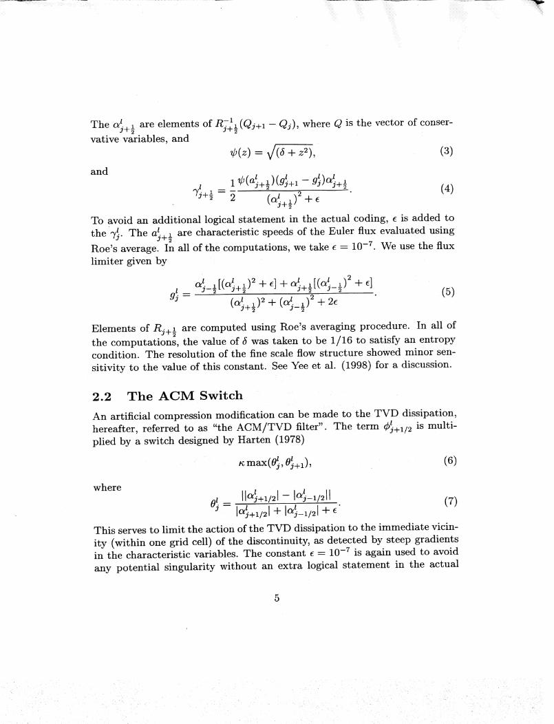
The c_L _ are elements of -1R+½ (Qj+I- Qj) where Q is the vector of conser-J+7
vative variables, and
¢(z) = v/(_+ z_), (3)and
__ l • l
J _ (4).y_+½ _ l¢(a(+_)(g}+_ gj)aj+½t 2
(%+½)+_To avoid an additional logical statement in the actual coding, e is added to
the @ The a Z. _ are characteristic speeds of the Euler flux evaluated using3" 3+g
Roe's average. In all of the computations, we take e -- 10 -7. We use the flux
limiter given by
d, [(._+ )_+_] + .' . [(.}_.)_ + 41 1 j-t-_ _ . (5)
(_+½
Elements of Rj+½ are computed using Roe's averaging procedure. In all of
the computations, the value of 5 was taken to be 1/16 to satisfy an entropycondition. The resolution of the fine scale flow structure showed minor sen-
sitivity to the value of this constant. See Yee et al. (1998) for a discussion.
2.2 The ACM Switch
An artificial compression modification can be made to the TVD dissipation,
hereafter, referred to as "the ACM/TVD filter". The term Ctj+_/2 is multi-
plied by a switch designed by Harten (1978)
1 l_ max(Oj, Oj+l), (6)
wherel l
0_:_ 11%+1/21- 1°9-1/211'- Ir---- .... r........ • (7)%+_!21 + 1%-_121+ e
This serves to limit the action of the TVD dissipation to the immediate vicin-
ity (within one grid cell) of the discontinuity, as detected by steep gradientsin the characteristic variables. The constant e- 10 -7 is again used to avoid
any potential singularity without an extra logical statement in the actual
.. >
;i}_i,:17• :_
ilililiiiiiiiiiiiiiiiii_'
iiliii!!_il
Method
CEN44
TVD22
TVD44
TVD66
ACM22
ACM44
ACM66
ACM44C
ACM66C
Order
(Euler)
Order
(viscous)4
2
4
6
2
4
6
4
6
Shock-
capturing
No ¸
Yes
Yes
Yes
Yes
Yes
Yes
Yes
Yes
Artificial
compression
No
No
No
No
Yes
Yes
Yes
Yes
Yes
Compact
No
No
No
No
No
! NoNo:
, Yes
Yes
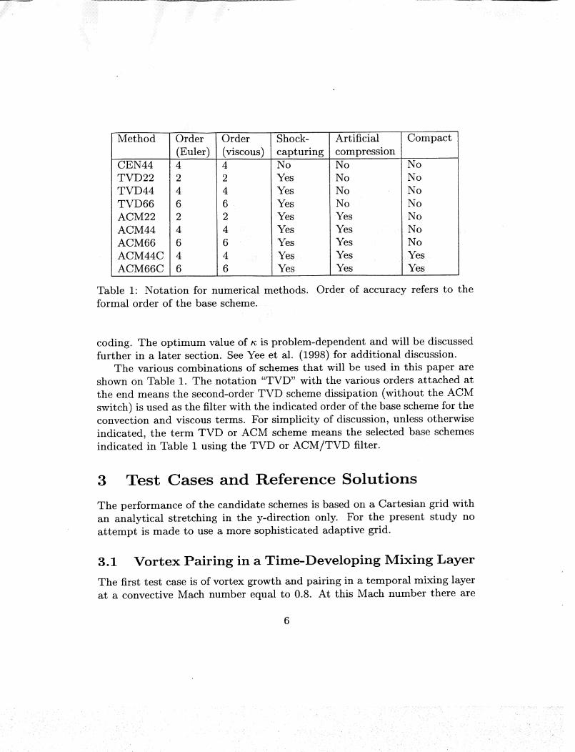
Table 1" Notation for numerical methods.
formal order of the base scheme ....
Order of accuracy refers to the
coding. The optimum value of _ is problem-dependent and will be discussed
further in a later section. See Yee et al. (1998) for additional discussion.
The various combinations of schemes that will be used in this paper are
shown on Table 1. The notation "TVD" with the various orders attached at
the end means the second-order TVD scheme dissipation (without the ACM
switch) is used as the filter with the indicated order of the base scheme for theconvection and viscous terms. For simplicity of discussion, Unless otherwise
indicated, the term TVD or ACM scheme means the selected base schemes
indicated in Table 1 using the TVD or ACM/TVD filter.
3 Test Cases and Reference Solutions
The performance of the candidate schemes is based on a Cartesian grid with
an analytical stretching in the y-direction only. For the present study no
attempt is made to use a more sophisticated adaptive grid.
3.1 Vortex Pairing in a Time-Developing Mixing Layer
The first test case is of vortex growth and pairing in a temporal mixing layer
at a convective Mach number equal to 0.8. At this Mach number there are
:i__
shock waves (shocklets) that form around the vortices and the problem is to
compute accurately the vortex evolution while avoiding oscillations aroundthe shocks. Previous calculations of the problem can be found in Sandham
and Reynolds (1989), Lumpp(1996a,b) and Fu and Ma (1997). Here we set
up a base flow as in Sandham and Yee (1989)
u -- 0.5 tanh(2y), (s)
with velocities normalized by the velocity jump U1- U2 across the shear layer
and distances normalized by vorticity thickness,
U_ - U2 (9)5_- (du/dy)ma_"
Subscripts 1 and 2 refer to the upper (y > 0) and lower (y < 0) streams of
fluid respectively. The normalized temperature and hence local sound speed
squared is determined from an assumption of constant stagnation enthalpy
c2 _ c2 + 3'- 12 (U2 -- u2)" (10)
Equal pressure through the mixing layer is assumed. Therefore, for this
configuration of U2 -- -U1 both fluid streams have the same density and
temperature for y --+ =kcx_. The Reynolds number defined by the velocity
jump, vorticity thickness and kinematic viscosity at the free-stream temper-ature is set here to be 1000. The Prandtl number is set to 0.72, the ratio of
specific heats is taken as V- 1.4 and Sutherland's law
]_t ._ (C2/C2R)1"5(1 + llO.3/TR) (11)
#R C2/C2R + 110.3/TR
with reference temperature TR -- 300K is used for the viscosity variation
with temperature. The reference sound speed squared c2 is taken as the
average of c2 over the two free streams with _tR the Viscosity corresponding
to c 2.
Disturbances are added to the velocity components in the form of simple
waves. For the normal component of velocity we have the perturbation
2
v' -- __, ak cos(27rkx/L_ + Ck) exp(--y2/b), (12)k=l
•.... ,- _ !_:i_!_I,_. _
: i ¸ : -
where L_ = 30 is the box length in the x-direction and b -- 10 is the
y-modulation. In our test case we simulate pairing in the center of the
computational box, by choosing the initially most unstable wave k -- 2 to
have amplitude a2 -- 0.05 and phase ¢2 ---_/2, and the subharmonic wave
k -- 1 with al -- 0.01 and ¢1 -- -7r/2. The u-velocity perturbations are
found by assuming that the total perturbation is divergence free. These
fluctuations correspond only approximately to eigenfunctions of the linear
stability problem for a compressible mixing layer, but they serve the purpose
of initiating the instability of the mixing layer and have the advantage as a
test case in that they can be easily coded.
Numerically the grid is equally spaced and periodic in the x-direction and
stretched in the y-direction, using the mapping
Ly sinh(by_) (13)Y-- 2 sinh(by) '
where we take the box size in the y-direction Ly -- 100, and the stretching
factor by -- 3.4. The mapped coordinate r] is equally spaced and runs from-1 to +1. The boundaries at -+-Ly/2 are taken to
at the lower boundary
be slip walls. For example,
Pl -- P2,
(pv) - o,(ET)_ - [4(ET)2-- (ET)a]/3,
(14)
(15)(16)
(17)
where subscripts here refer to the grid point and ET is the total energy.
Sample results for this configuration were obtained from computations on
a 201 x 201 grid, using the fourth-order non-compact central spatial differ-
encing, and the ACM/TVD filter (ACM44). The constant n=0.7 for theu + c and v + c nonlinear characteristic fields and n=0,35 for the u and v
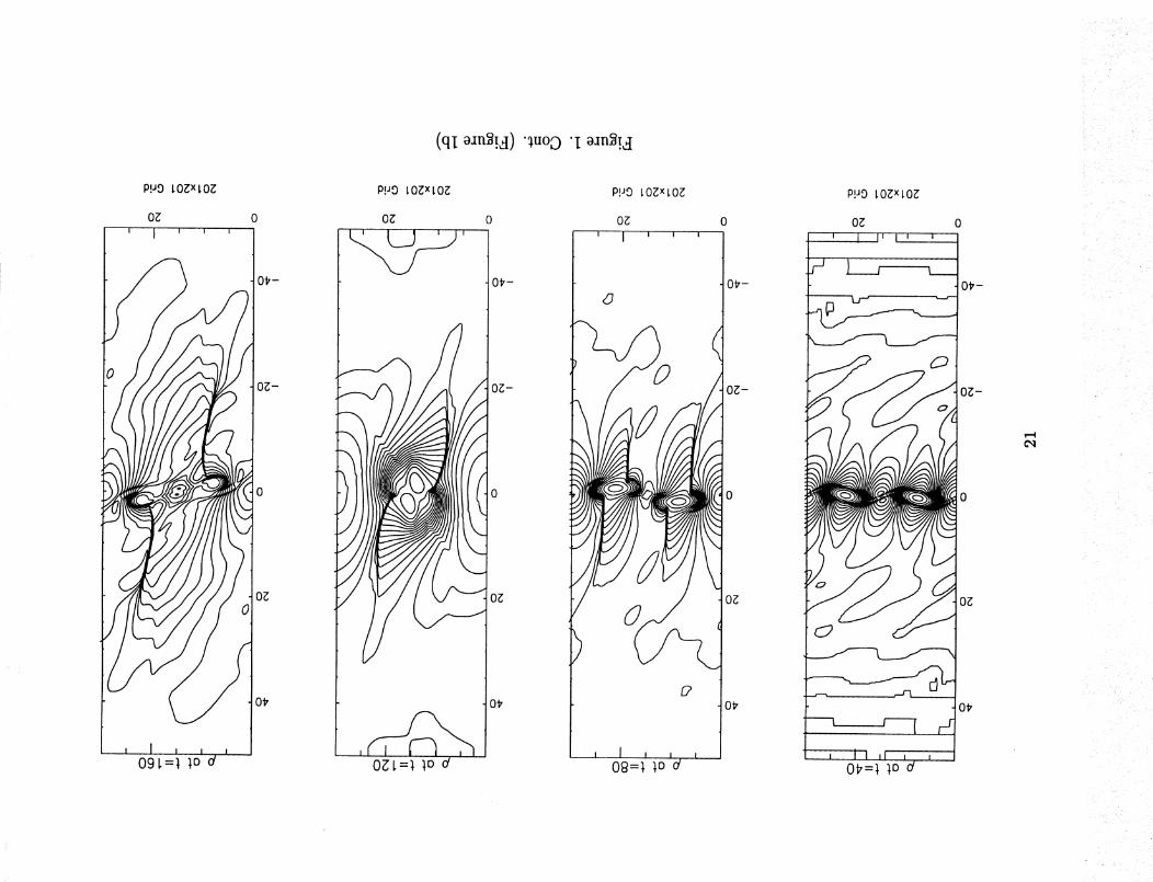
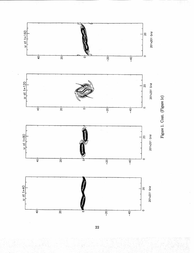
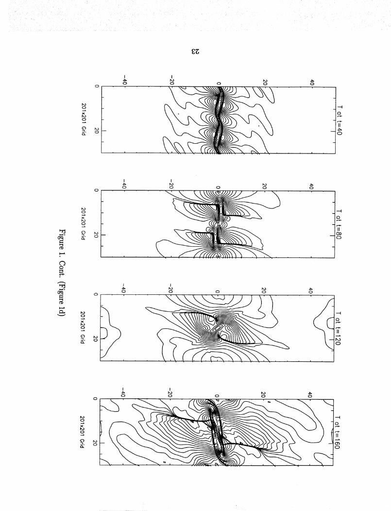
linear characteristic fields were used for the computations. Figure la shows
snapshots of the pressure field at times t -- 40, 80,120,160, illustrating the
roll-up of the primary vortices, followed by vortex merging. Figure lb - ldshow the corresponding density, vorticity and temperature contours. Shock
waves form around the vortices, with a peak Mach number ahead of the vor-
tex of approximately 1.55 at t -- 120. Figure 2 shows the growth of two
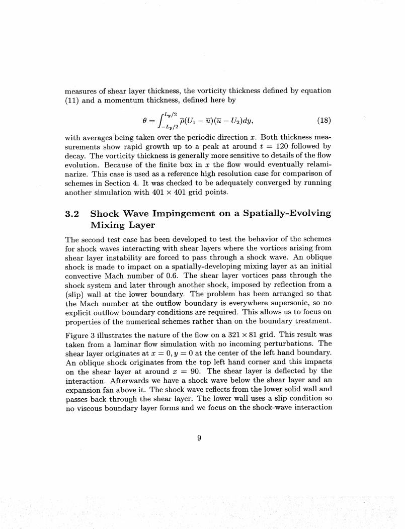
measuresof shearlayer thickness,the vorticity thicknessdefinedby equation(11) and a momentum thickness,defined here by
fLy�2-- j_L_/2"p(UI_ -- _)(_- U2)dy, (18)
with averages being taken over the periodic direction x. Both thickness mea-
surements show rapid growth up to a peak at around t -- 120 followed by
decay. The vorticity thickness is generally more sensitive to details of the flowevolution. Because of the finite box in x the flow would eventually relami-
narize. This case is used as a reference high resolution case for comparison of
schemes in Section 4. It was checked to be adequately converged by running
another simulation with 401 x 401 grid points.
Shock Wave Impingement on a Spatially-Evolving
Mixing Layer
The second test case has been developed to test the behavior of the schemes
for shock waves interacting with shear layers where the vortices arising from
shear layer instability are forced to pass through a shock wave. An oblique
shock is made to impact on a spatially-developing mixing layer at an initial
convective Mach number of 0.6. The shear layer vortices pass through the
shock system and later through another shock, imposed by reflection from a
(slip) wall at the lower boundary. The problem has been arranged so that
the Mach number at the outflow boundary is everywhere supersonic, so no
explicit outflow boundary conditions are required. This allows us to focus on
properties of the numerical schemes rather than on the boundary treatment.
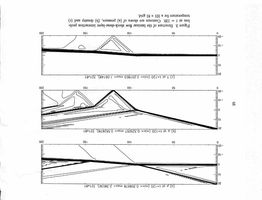
Figure 3 illustrates the nature of the flow on a 321 x 81 grid. This result was
taken from a laminar flow simulation with no incoming perturbations. The
shear layer originates at x -- 0, y -- 0 at the center of the left hand boundary.
An oblique shock originates from the top left hand corner and this impacts
on the shear layer at around x- 90. The shear layer is deflected by the
interaction. Afterwards we have a shock wave below the shear layer and an
expansion fan above it. The shock wave reflects from the lower solid wall and
passes back through the shear layer. The lower wall uses a slip condition so
no viscous boundary layer forms and we focus on the shock-wave interaction
Property (1) (2) (3) (4) (5)u-velocity
v-velocity
0 (degrees)
density p
pressure p
sound speed c
Mach number IMI
3.0000
0.0000
0.0000
1.6374
0.3327
0.5333
5.6250
2.0000
0.0000
0.0000
0.3626
0.3327
1.1333
1.7647
2.9709
-0.1367
2.6343
2.1101
0.4754
0.5616
5.2956
2.9792
-0.1996
3.8330
1.8823
0.4051
0.5489
5.4396
1.9001
-0.1273
3.8330
0.4173
0.4051
1.1658
1.6335
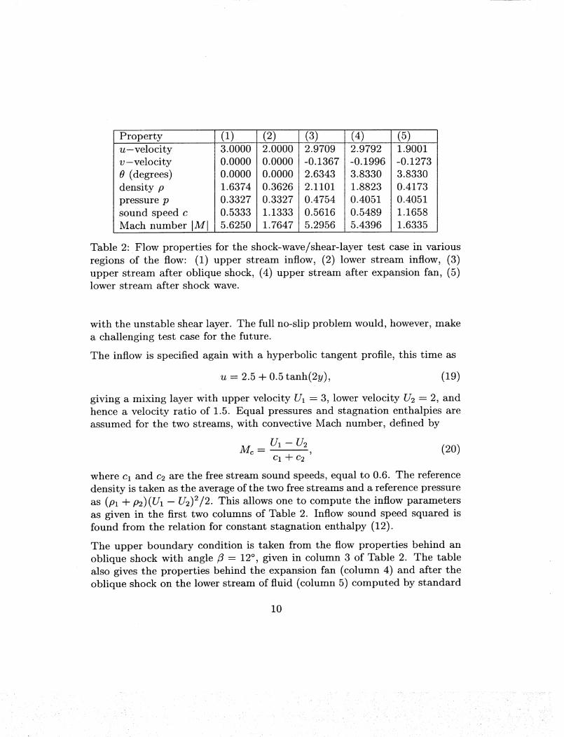
Table 2: Flow properties for the shock-wave/shear-layer test case in various
regions of the flow: (1) upper stream inflow, (2) lower stream inflow, (3)
upper stream after oblique shock, (4) upper stream after expansion fan, (5)
lower stream after shock wave.
with the unstable shear layer. The full no-slip problem would, however, make
a challenging test case for the future.
The inflow is specified again with a hyperbolic tangent profile, this time as
u -- 2.5 + 0.5 tanh(2y), (19)
giving a mixing layer with upper velocity U_ -- 3, lower velocity U2 -- 2, and
hence a velocity ratio of 1.5. Equal pressures and stagnation enthalpies are
assumed for the two streams, with convective Mach number, defined by
(20)ci +c2
where c_ and c2 are the free stream sound speeds, equal to 0.6. The reference
density is taken as the average of the two free streams and a reference pressure
as (p_ + p2)(U_ - U2)2/2. This allows one to compute the inflow parameters
as given in the first two columns of Table 2. Inflow sound speed squared isfound from the relation for constant stagnation enthalpy (12).
The upper boundary condition is taken from the flow properties behind an
oblique shock with angle/_ -- 12 °, given in column 3 of Table 2. The table
also gives the properties behind the expansion fan (column 4) and after the
oblique shock on the lower stream of fluid (column 5) computed by standard
10
: • i!i_!i_iiiii_i!_i i!i_ii_i _iJ̧ I_¸¸ii_ili ii
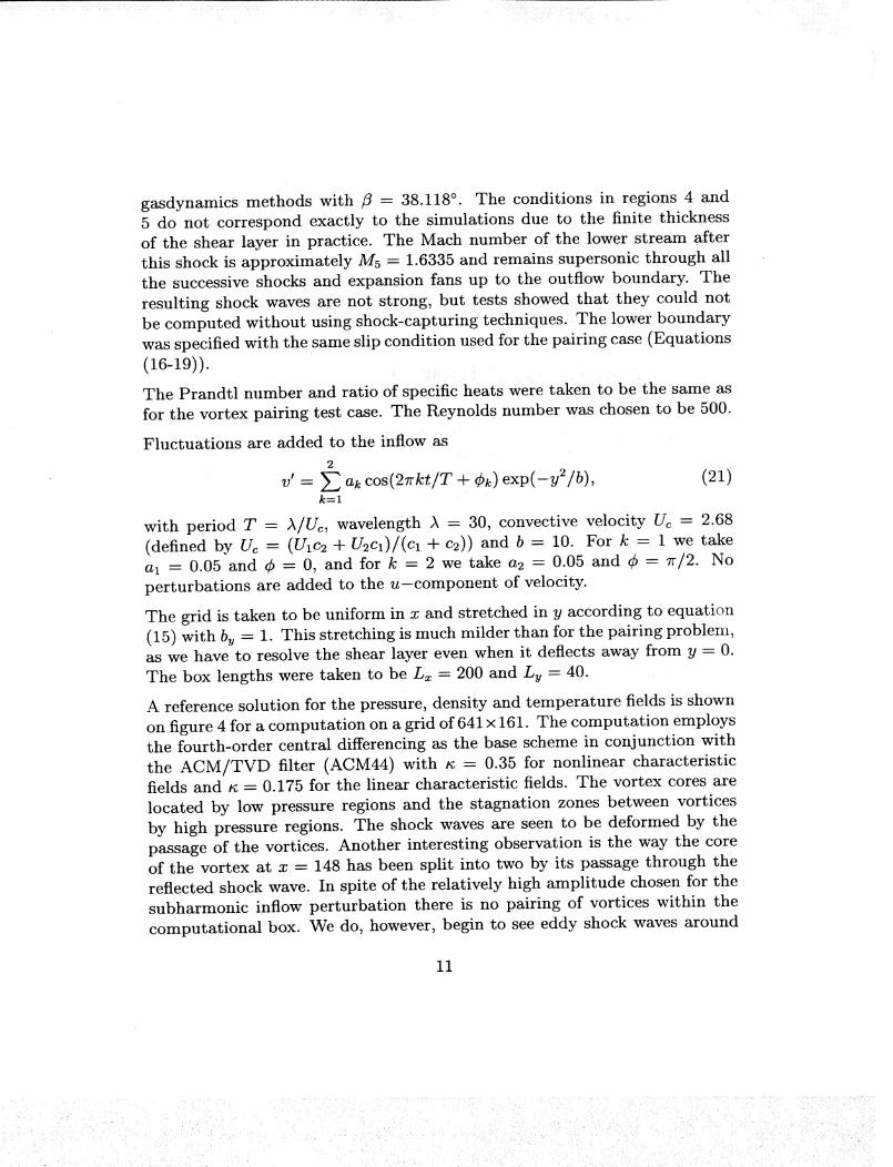
gasdynamics methods with fl = 38:.118 °. The conditions in regions 4 and
5 do not correspond exactly to the simulations due to the finite thickness
-of the shear _layer in practice, The Math number of the lower stream after
this shock is approximately M_ = 1.6335 and remains supersonic...... through....... all
the successive shocks and expansion fans up to the outflow boundary. The
resulting shock waves are not strong, but tests showed that they could not
be computed without using shock-capturing techniques. The lower boundary
was specified with the same slip condition used for the pairing case (Equations
( 16-19) ). : : .....The Prandtl number and ratio of specific heats were taken to be the same as
for the vortex pairing test case The Reynolds number was chosen to be 500.
Fluctuations are added to the inflow as
2
v' __, ak cos(2_rkt/T + Ck)exp(--Y_/b),k=I
(21)
with period T- /k/U_, wavelength _k- 30, convective velocity U_ -- 2.68
(defined by Uc- (ULC2-4-U2Cl)/(c1-4" c2))and b- 10. For k -- 1 we takeal -- 0.0'5 and ¢-- 0, and for k -- 2 we take a2 -- 0.05 and ¢-- _r/2. No
perturbations are added to the u-component of velocity.
The grid is taken to be uniform in x and stretched in y according to: equation
:(15) with b_ -- 1. This stretching is much milder than for the pairing problem,as we have to resolve the shear layer even when it deflects away from y- 0.
The box lengths were taken to be/-,x = 200 and/.,_ = 40.
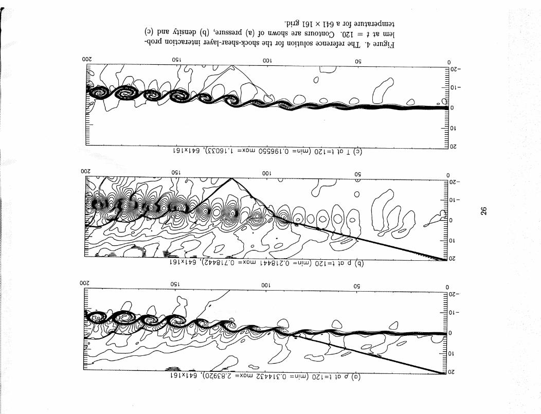
A reference solution for the pressure, density and temperature fieldsis shown
on figure 4 for a computation on a grid of 641 x 161. The computation employsthe fourth-order central differencing as the base scheme in conjunction with
the ACM/TVD filter (ACM44) with _ -- 0.:315 for nonlinear characteristicfields and _- 0.1715 for the linear characteristic fields. The vortex cores are
located by low pressure regions and the stagnation zones between vortices
by high pressure regions. The shock waves are seen to be deformed by the
passage of the vortices. Another interesting observation is the way the coreof the vortex at x -- 148 has been split into two by its passage through the
reflected shock wave. In spite of the relatively high amplitude chosen for the
subharmonic inflow perturbation there is no pairing of vortices within the
computational box. We do, however, begin to see eddy shock waves around
11
the vortices near the end of the computational box wherethe local convectiveMach number has increasedto around 0.66. The oscillations seennear theupper boundary for x > 120 occur where the small Mach waves from the
initial perturbations arrive at the upper boundary. The use of characteristic
boundary conditions should remove this problem. Practically, the amplitudeof oscillations is not sufficient to cause numerical instability or affect the
remainder of the flow.
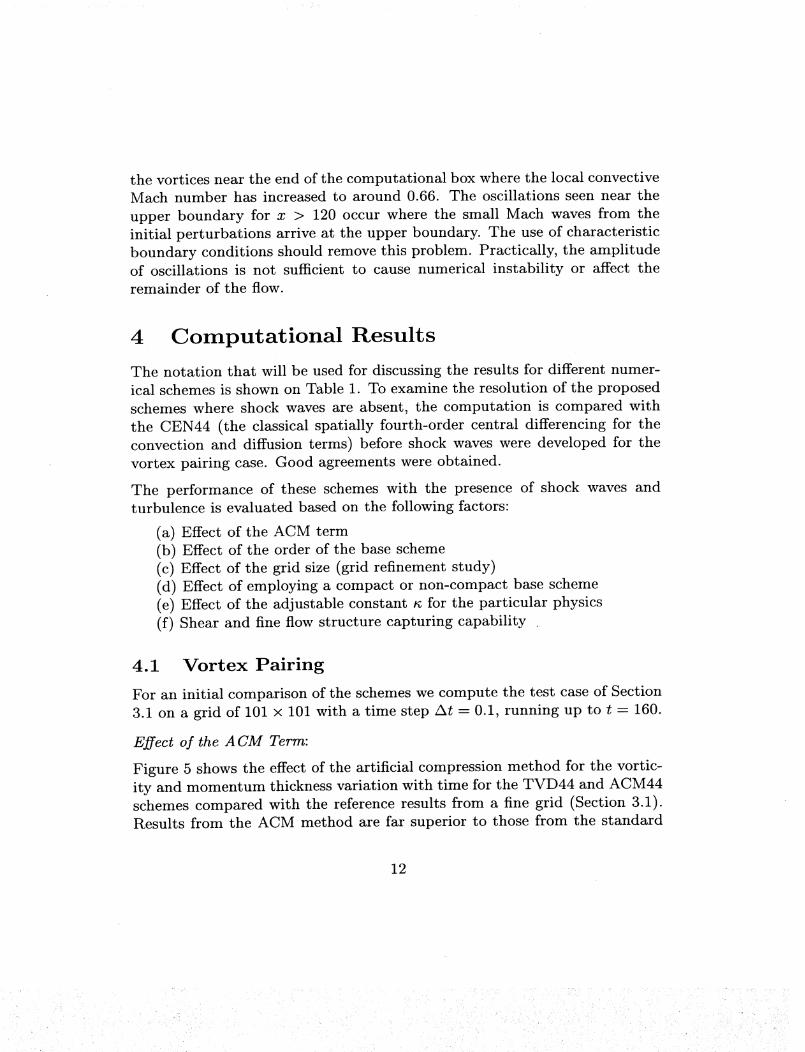
4 Computational Results
The notation that will be used for discussing the results for different numer-
ical schemes is shown on Table 1. To examine the resolution of the proposed
schemes where shock waves are absent, the computation is compared with
the CEN44 (the classical spatially fourth-order central differencing for the
convection and diffusion terms) before shock waves were developed for the
vortex pairing case. Good agreements were obtained.
The performance of these schemes with the presence of shock waves andturbulence is evaluated based on the following factors"
(a) Effect of the ACM term
(b) Effect of the order of the base scheme
(c) Effect of the grid size (grid refinement study)
(d) Effect of employing a compact or non-compact base scheme
(e) Effect of the adjustable constant n for the particular physics
(f) Shear and fine flow structure capturing capability
4.1 Vortex Pairing
For an initial comparison of the schemes we compute the test case of Section
3.1 on a grid of 101 x 101 with a time step At -- 0.1, running up to t -- 160.
Effect of the A CM Term:
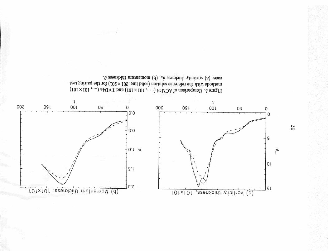
Figure 5 shows the effect of the artificial compression method for the vortic-
ity and momentum thickness variation with time for the TVD44 and ACM44
schemes compared with the reference results from a fine grid (Section 3.1).
Results from the ACM method are far superior to those from the standard
12
:: :: .... i ¸ •
_i!!_i_i_ii<̧!i!ii!_....._......!::<_:<:< <<%<i_)!i.......! <!!iii<<_i_iiiii<
TVD formulation. Note that there is no improvement in the shock resolu-
tion since the ACM term limited the amount of dissipation away from high
gradient areas whereas the shock resolution is dictated by the flux limiter.
Effect of the Order of the Base Scheme:
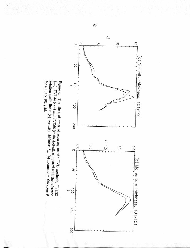
Figure 6 shows the effect of increasing accuracy from second to fourth and
sixth order using the TVD filter (TVD22, TVD44 and TVD66). As can be
seen there is almost no improvement as the order of accuracy is raised. Fig-
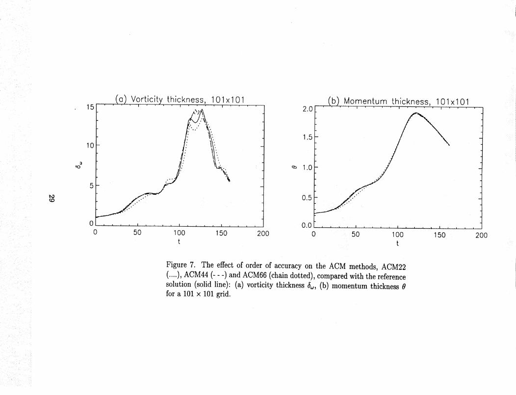
ure 7 shows the same plot for the ACM/TVD filter (ACM22, ACM44 and
ACM66). Here there is an improvement, although the results even for the
lowest order are quite good. There is little to choose in the shock resolution
properties with the variation in order of accuracy. We choose to compare
temperature contours, which are most sensitive to oscillations (Lumpp, pri-
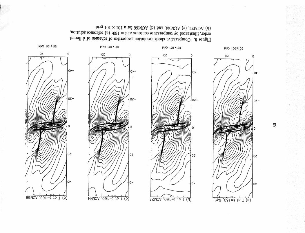
vate communication). Figure 8 shows a comparison of the ACM schemes of
various order with the reference solution. All the schemes here capture theshock waves with minimal oscillations. The temperature contours for the
TVD filter of the various order using a 101 x 101 grid, although not shown,
are not even nearly as accurate asthe ACM44 using a 41 x 41 grid. See the
last plot of Figure 15 for a comparison. It can be seen that there is a sig-nificant advantage in moving from second to fourth order, but less is gained
in moving from fourth to sixth order using TVD or ACM/TVD as a filter.This is in contrast' to an isentropic vortex convection test case where there
are definite benefits of moving from fourth order to sixth order (Yee et al.,
1998). It appears that the effect of order of accuracy are more pronounced
for long time integrations of pure convection.
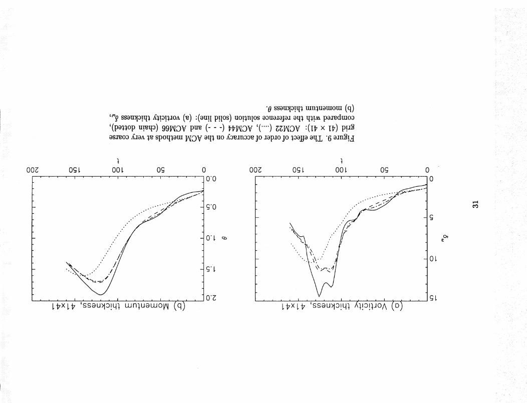
Effect of the Grid Size (Grid Refinement Study)"
To investigate the effect of order of the accuracy in more detail we consider
simulations on a very coarse grid of 41 x 41 points. Such a case corresponds
in practice to simulation of scales of turbulence arising from shear layers only
two or three computational cells across. Figure 9 shows results for the ACMschemes To ensure that the fine scale flow structure is fully resolved by the
reference grid 201 x 201, the same simulation was done on a 401 x 401 grid
(figures not shown).
13
Effect of Compact or Non-Compact Base Scheme:
For wave propagation and computational problems the performance of fourth
and sixth-order compact schemes, although more CPU intensive, appears to
be superior to their non-compact cousin. For problems with shock waves the
benefit of compact over non-compact schemes is less known due to the filter
step. Figure 10 shows results for the fourth and sixth-order compact schemes,
which are similar to results from the sixth-order non-compact scheme. Again
there is little improvement compared with the fourth-order non-compact
scheme. A conclusion is that the use of the ACM/TVD in the filter step
is essential to get the benefits of moving from second to fourth order, but
even with this method there is little benefit in moving to even higher-order
schemes.
Effect of the Adjustable Constant _:
The ACM switch of Harten has been demonstrated to give good shock resolu-
tion and to be essential if the benefits of higher-order discretization schemes
are to be realized. There is, however, an adjustable parameter _ in the for-
mulation, and results are sensitive to the precise choice of its value. Figure
11 illustrates the effect on the result for the pairing test case of reducing the
parameter from 0.7 to 0.35. The vorticity and momentum thickness devel-
opment is improved due to the reduction in numerical dissipation From the
temperature contours on Figure 12 it can be seen that this has been achievedat the cost of formation of small oscillations around the shock wave. For the
present problem one would be ready to pay this price to get the more accurate
vortex evolution. However, in general it is not known how such numerically-induced oscillations interact with small scales of turbulence. For the current
method the correct procedure for a simulation of shock-turbulence interac-
tion would be to find the smallest value of _ to resolve the shock waves
satisfactorily and then increase the grid resolution until the turbulence is ad-
equately resolved. There are perhaps other formulations of the ACM switch
parameter _ based on the flow physics that can perform the adjustment to
higher values automatically when stronger shock waves are present. This is
a subject of future research.
Shear and Fine Flow Structure Capturing Capability:
Shock-capturing schemes are designed to accurately capture shock waves, but
14
with a lessaccurate capturing capability for contact discontinuities. In fact,the mixing layer seenat a large scaleis a contact discontinuity. If one usesenough grid points to resolvethe region of high shear in conjunction withphysical viscosity, it might not needto be 'captured'. Contact discontinuitiesrelate to the characteristic velocities u and v. As an experiment these linear
characteristics were computed with no numerical dissipation. Filters were
only applied to the nonlinear characteristics fields u ± c and v ± c using the
ACM44 method. Interestingly, the computation was no less stable than that
the full TVD or ACM schemes (applying _ to all of the characteristic fields).
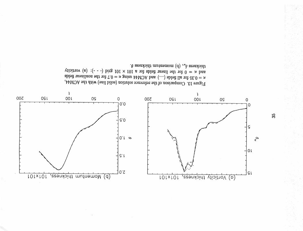
Figure 13 shows the vorticity thickness evolution and Figure 14 the resulting
temperature field. It can be seen that good results were obtained, althoughthere is a trace of oscillation near the shock wave. This could be remedied
by increasing _ slightly. See Yee et al. (1998) for an illustration. However,the flow features of the shear and fine flow structure are accurately captured
with similar resolution as the 201 x 201 grid with ACM44 applied to all of
the characteristic fields (Figure 1ha).
To balance the shear and shock-capturing, one alternative is to switch to a
more compressive limiter (see Yee (1989)) for the linear characteristics fields.Another alternative is to reduce the value of _ for the u, v linear fields. The
comparison of using different values of t_ for the linear and nonlinear fields is
also shown in Figures 13 and 14.
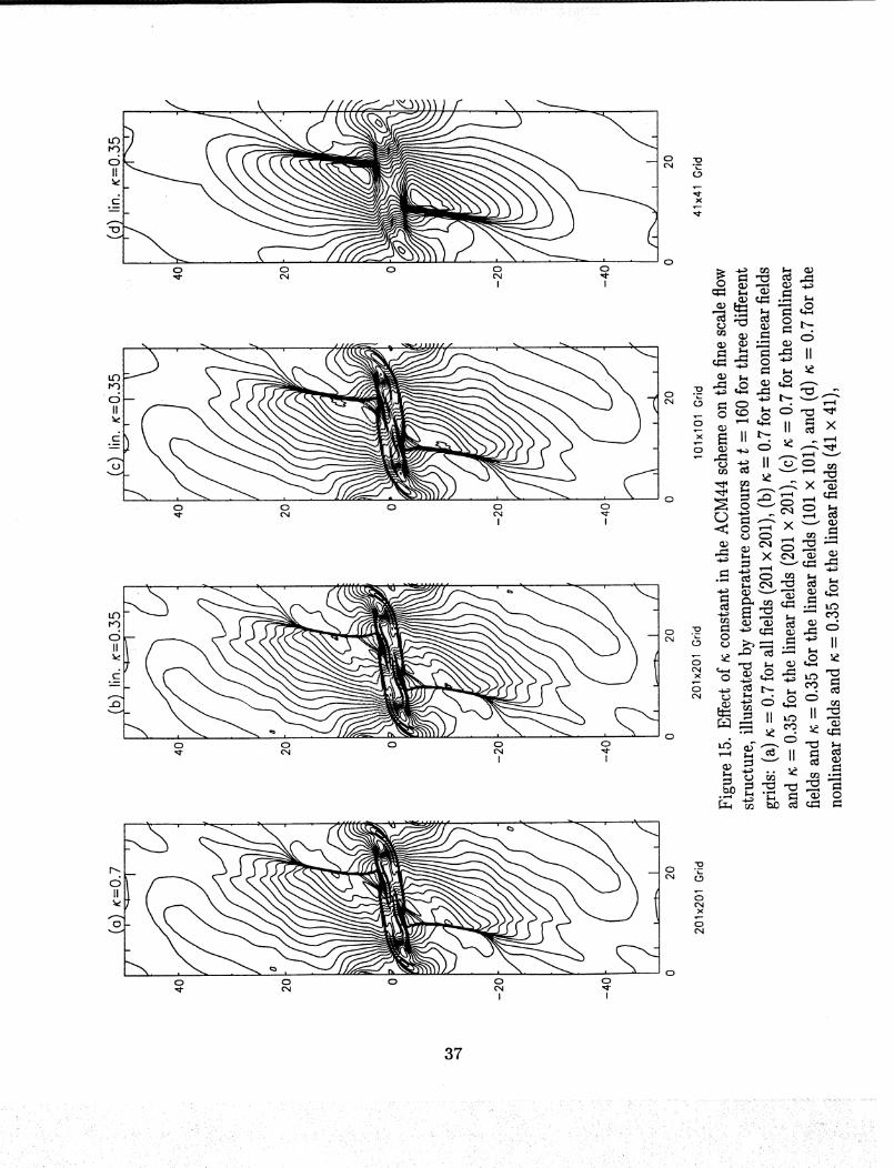
Figure 15 shows the comparison of the different n values for the three grids.
Figure 16 shows the comparison of the five classical flux limiters (see Equa-
tions (4.34c)-(4.34g) of Yee (1989)) using ACM44.
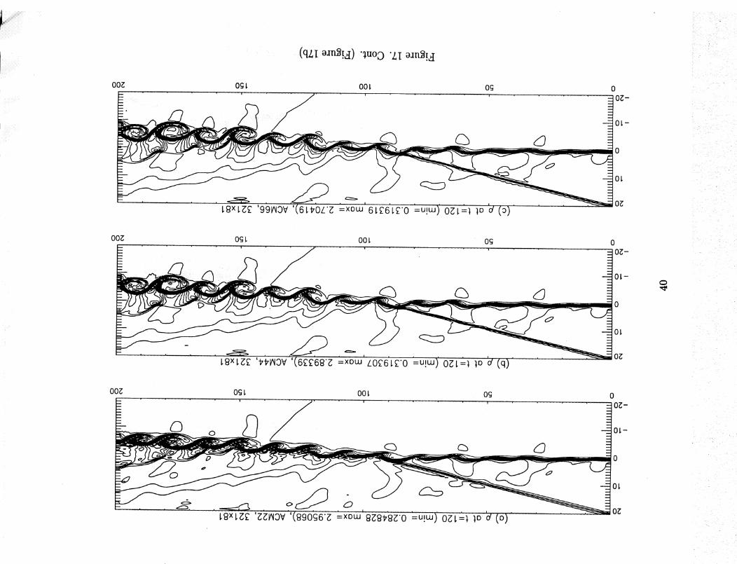
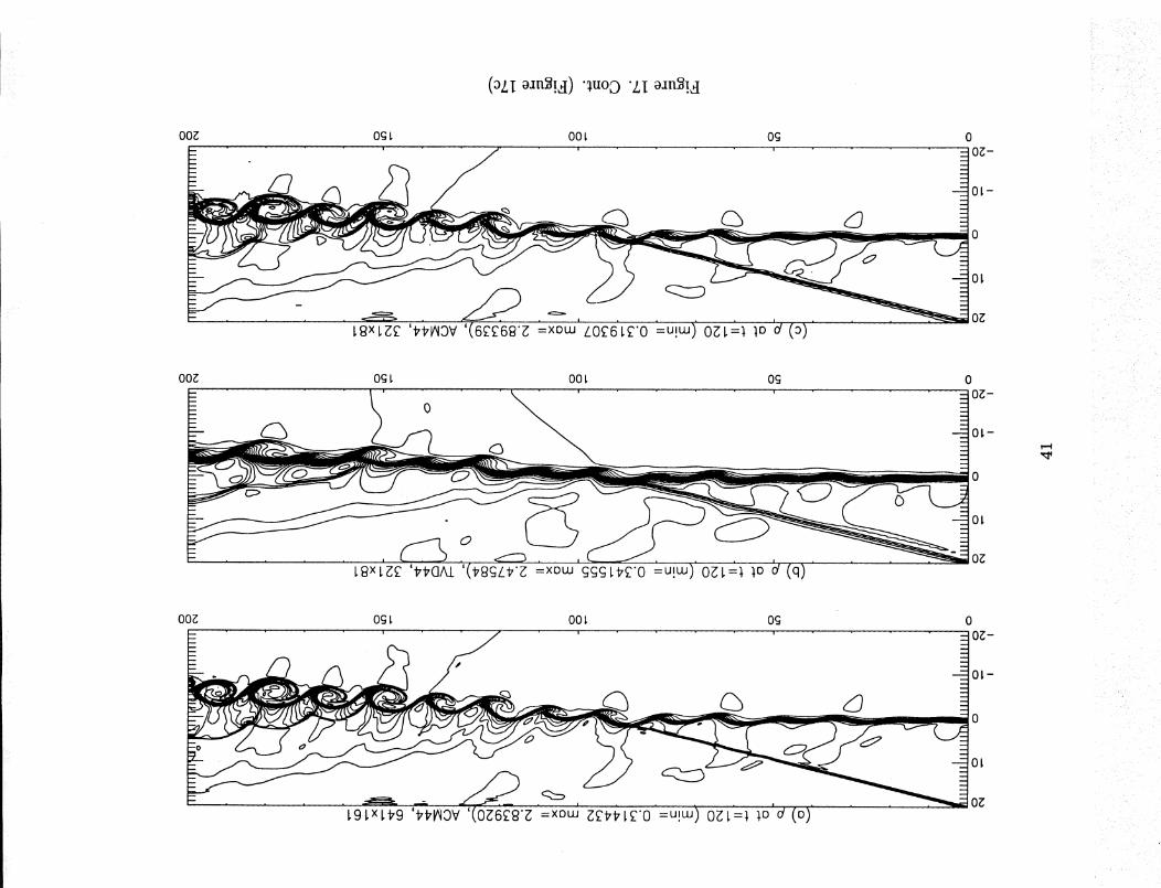
Shock-Shear Layer Interaction
The test case defined in Section 3.2 was run on a grid of 321 x 81 with
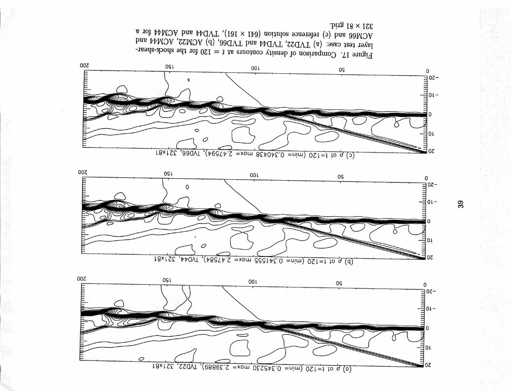
At -- 0.12 up to t -- 120 with n -- 0.35. Figure 17 shows the density fieldfor the TVD44 and ACM44 schemes compared with the reference solution
(641 x 161 grid). Again it can be seen that the ACM modification is essential
for obtaining good vortex evolution (additionally better shock resolution is
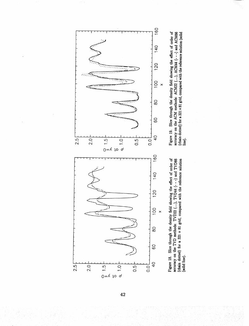
obtained). For a more quantitative comparison Figures 18 and 19 show slices
through the density field between x --50 and x 150 at y -- 0 (the centerline
of the computational domain). From Figure 18 it is apparent that all the
standard TVD schemes, of whatever order, miss the correct vortex formation.
15
_i_ i._ _i_i:i
Method
Method
CEN44
TVD22
TVD44
ACM22
ACM44
Pairing
(200 steps)
19.5
18.8
23.4
19.6
24.2
Shock-wave
(100 steps)22.1
22.8
26.9
23.8
27.9
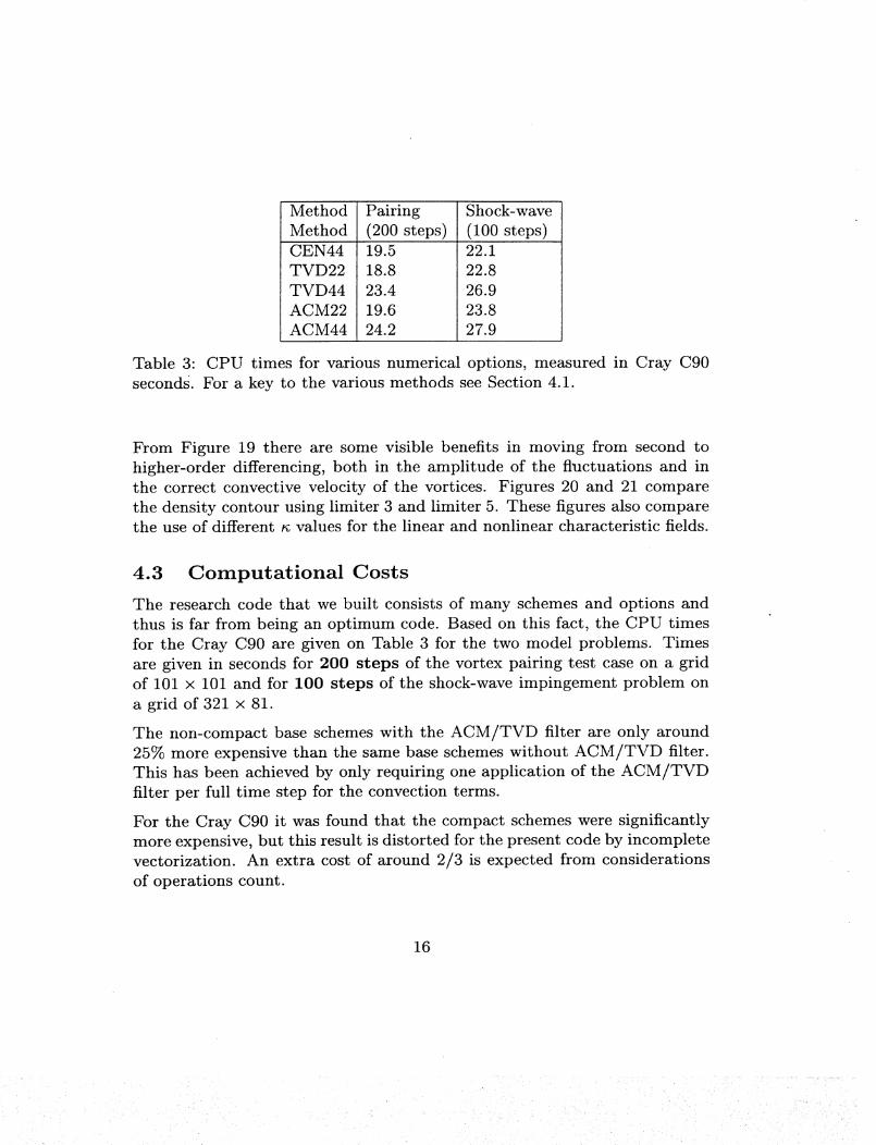
Table 3: CPU times for various numerical options, measured in Cray C90
seconds. For a key to the various methods see Section 4.1.
From Figure 19 there are some visible benefits in moving from second to
higher-order differencing, both in the amplitude of the fl_actuations and in
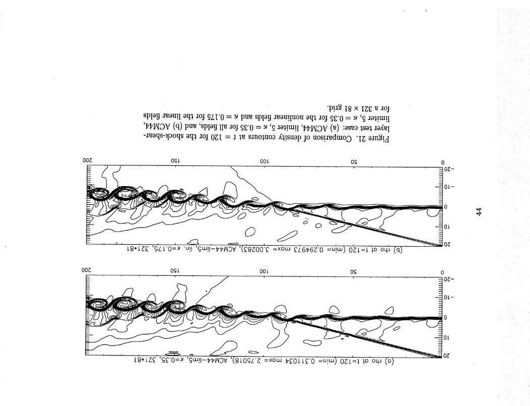
the correct convective velocity of the vortices. Figures 20 and 21 compare
the density contour using limiter 3 and limiter 5. These figures also comparethe use of different _ values for the linear and nonlinear characteristic fields.
4.3 Computational Costs
The research code that we built consists of many schemes and options and
thus is far from being an optimum code. Based on this fact, the CPU times
for the Cray C90 are given on Table 3 for the two model problems. Times
are given in seconds for 200 steps of the vortex pairing test case on a grid
of 101 × 101 and for 100 steps of the shock-wave impingement problem on
a grid of 321 × 81.
The non-compact base schemes with the ACM/TVD filter are only around
25% more expensive than the same base schemes without ACM/TVD filter.
This has been achieved by only requiring one application of the ACM/TVD
filter per full time step for the convection terms.
For the Cray C90 it was found that the compact schemes were significantly
more expensive, but this result is distorted for the present code by incomplete
vectorization. An extra cost of around 2/3 is expected from considerations
of operations count.
16
i _ , _ •
5 Conclusions
Two model problems were considered to test the behavior of shock-capturing
schemes in flows where the evolution of vortices from shear layer instabilities
plays a crucial role. Standard total variation diminishing schemes do not
perform well for these problems. It was found that an artificial compression
modification gave much improved results and with this approach there are
definite benefits in moving from second to fourth-order differencing schemes.
The benefits were less pronounced in moving to sixth order The fourth order
ACM44 schemes show highly accurate shock-wave and shear-layer capability.
The non-compact fourth-order base scheme requires a five point stencil, the
same as the second-order TVD _scheme. There is potentially an additional
problem near boundaries in that reduced order and/or upwind schemes must
be used. Stable boundary conditions such as those proposed by Gustafs-
son and Olsson (1995) must be applied. If an adaptive grid is used, higher
accuracy can be obtained.
Acknowledgment: The major portion of the work of the first author was
performed as a visiting scientist at RIACS, NASA Antes Research Center.
Special thanks to Marcel Vinokur and M. Jahed Djomehri for their critical
review of the manuscript.
References
Adams, N.A. 1997 Direct numerical simulation of turbulent supersonic bound-
ary layer flow. First AFOSR International Conference on DNS and LES,
Ruston, LA, USA.
Adams, N.A. and Shariff, K. 1996 A high-resolution hybrid compact-ENO
scheme for shock-turbulence interaction problems. J. Comput. Phys. 127,
27-51.
Alam, M. and Sandham, N.D 1997b Numerical study of separation bubbles
with turbulent reattachment followed by a boundary layer relaxation. Par-
allel Computational Fluid Dynamics '97 (Ed. A. Ecer et al.), Elsevier, to
appear.
Ciment, M. and Leventhal, H. 1975 Higher order compact implicit schemes
for the wave equation, Math. Comp. 29, 985-994.
17

Fu, D. and Ma, Y. 1997A high order accuratedifferenceschemefor complexflow fields. J. Comput. Phys. 134, 1-15. Gustafsson, B. and Olsson, P. 1995
Fourth-order difference methods for hyperbolic IBVPs. J. Comput. Phys.
117, 300-317.
Gustafsson, B and Olsson, P. 1995 Fourth-order difference methods for hy-
perbolic IBVPs. J. Comput. Phys. 117, 300-317.
Harten, A. 1978 The Artificial compression method for computation of shocks
and contact discontinuities" III Self-adjusting hybrid schemes, Math, Comp.
32, 363-389.
Hirsh, R.S. 1975 Higher order accurate difference solutions of fluid mechanics
problems by a compact differencing technique, J. Comput. Phys. 19, 90-109.
Hixon, R. and Turkel, E. 1998 High-accuracy compact MacCormack-type
schemes for computational aeroacoustics. AIAA paper 98-0365, 36th Aerospace
Sciences Meeting _ Exhibit, Jan. 12-15, Reno, NV.
Lele, S. 1992 Compact finite-difference schemes with spectral-like resolution.
J. Comput. Phys. 86, 187-210.
Lumpp, T. 1996a A critical review of high-order accurate finite volume ENO-
schemes. First Intl. Symposium on Finite Volumes for Complex Applications,
Rouen, France, July 14-17.
Lumpp, T. 1996b Compressible mixing layer computations with high-order
ENO schemes. 15th Intl. Conf. on Num. Meth. in Flui Dynamics, Monterey,June 1996.
Luo, K.H. and Sandham, N.D. 1994 On the formation of small scales in a
compressible mixing layer. In Direct and Large-Eddy Simulation I, Kluwer
Academic Publishers, 335-346.
Moin, P. and Mahesh, K. 1998 Direct numerical simulation" a tool in turbu-
lence research. Ann. Rev. Fluid Mech. 30, 539-578.
Sandham, N.D. and Reynolds, W.C. 1989 A numerical investigation of the
compressible mixing layer. Report TF-g5, Department of Mechanical Engi-
neering, Stanford University.
18
k •
Sandham, N.D., and Reynolds, W.C. 1991 Three-dimensional simulations of
large eddies in the compressible mixing layer. J. Fluid Mech. 224, 133-158.
Sandham, N.D. and Yee, H.C. 1989 A numerical study of a class of TVD
schemes for compressible mixing layers. NASA Technical Memorandum 10219_.
Vreman, B., Kuerten, H., and Geurts, B. 1995 Shocks in direct numericalsimulation of the confined three-dimensional mixing layer. Phys. Fluids, to
appear.
Vreman, A.W., Sandham, N.D and Luo, K.H. 1996 Compressible mixing
layer growth rate and turbulence statistics. J. Fluid Mech., 320, 235-258.
Yee, H.C. 1989 A class of high-resolution explicit and implicit shock-capturing
schemes NASA Technical Memorandum 101088
Yee, H. C. 1997 Explicit and implicit multidimensional compact high-resolution
shock-capturing methods" Formulation J. Comput. Phys. Vol. 131 No. 1,
216-232.
Yee, H. C., Sandham, N. D. and Djomehri, M. J. 1998, Low dissipative high
order shock-capturing methods using characteristic based filters. RIACS
Technical Report 98.11, May 1998, NASA Ames Research Center.
19

0I,.0,r---
II
0
13_
0
II
o
13_
| I
0 0 0 0 0
I I
.'9_o _.
o
0
II
o
0 0 0 0 0C,,I C,,I
I I
.X2o ,_,,t--o
x
o
o
2O
P!J9 I,OZ:XI.OZ'
0;_
09L=l lo
o#-
o_-
o_
o_
(qI o_n_tA) "_uoo "I o_nlt!_I
P!J9 I.O_'XI.OE
O_I -- 1 I
P!J9 LO_x I,OZ_
I
,0
A
,,K Fq ,%OEL-1 lo d
O_5:'
0/=1 t lo_d .....L_
0_-
0_-
O_
O_
P!JO t O_x LO_
O_ 0
i ' l:J' I,', I
J 1.........., L__
. ,
0_'-
0_-
0
O_
O_
¢'Xl
•iiiiiiii!_ili¸ i¸•,
O
II
o
:3
, . . . . , • . . , .
| I I .
o o o o
I I
"10
x
Ocxl
I1'
o
O00II
o
, I
O
! i i i
O O O O
I I
oi_ • • I IO O
O_1 C_I ._-
I I
o
"ID°_
r_
o
x
O
C',I
.'2_o
OCN
x
O
°,,-i
OC)
,-4
.,,-i
O
II
o
iO o o
I I
"ID
i,..
r_
O
Oqx
O
Oq
22
I I
o o o o oo
_o"__i_ " ........ _'_o
I I
0 0 0 0 0
0.--LX
o
Crq
CD
o
_°
0_
I I4_ I'_ _ 4_.o o o o o
oL .....
o
--I
Q
I!(Do0 ¸
I I
0 0 0 0 00 _i
o Ii
&-
• ....
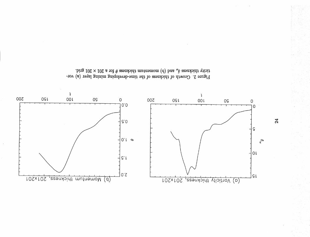
'P!:[_IO_x IO__ ao30 ssomp!q_mn_uomom (q)puu _)ssou_p!q_,{_!o!_
-aOA (_) aOA_I _Ut.XI.tU_ut.doloAop-otut._ oq_ jo ssou_p!q_ jo q_,_oa o "_; oan_!d
I
Og L O0 L' ' ' _ I ' " ' " l
1
Og 0 00_ OCjI, O0 L' ' ' '_ ' ' ' "--'_--0"0 " ' ' ' , ..... ' , '
O'L ,:::b
/--X_
,,,, :,,, q ,q,,,'_j' ( )LO_xLo_ ssau>1o!I o. OA
Og 0' ' ' I " ' • ......-r------- O
-OL
...... i gL
i__ .- _ _i!/!i/___ _i
00_ OgL OOL Og 0
' ' OE-
og L O0 L og| !
01,-
OL
OL
tO¢q
•pla_ I9I x Ilz9 _ aoj asn_aodtuaa
(a)pu_Xa,.suop(q) 'oanssoad(_)jo u_,oqsoa_sano_uoa "O_I- __ =°[-qoad uo!aa_ao:lu! aoX_i-a_oqs-)Iaoqs oqg, aoj uo!_nlos oauoaojoa oq& "p oan_!d
OOi_ og L O0 L og
..... L'9I.Xl,lz9 '(£'£'091,'1. =xow OCjg96L'O =U!LU) O_3L=),_o 1 (:))
00_Og _ O0 L Og 0
OL
O_
OL-
OL
C3 _3
..... i9i-xi,,-9'(6_.6_g_=xow _r;_,L_o =u!C_)OaL=_Bo_ (_,)
co
i_i:_i/__iii_'/!_il/•_i!_ _!_ _i: _,_
2
iii!iiLii_ :ili:
• _f_ i _ ,;,,
iili_'ili_i_iiiiiiiiiiiiiiiii!ii_i!_
iiii::i:ii!i!i!iii_i_!iiiiiiiii!_i,:,::
ii :iiiiiiiiiiiiiii_iiiii_i:i
iili!ili!iiiiiii!i!_ii'!_!_!i:
ii....
Og L...... '............1.........' ' '::': '.... 1 ' • ' "' ' "/_ ' '' ' '
_- . _o- j
..... _ t',/.... q
............ " t g" L
ii!!iiiiiiiiiiiii)iiiiiiiiiiiii:_........ /
I,0 I,x I,0 I, 'ssau>lolqt_...... cun),uaLu::OlAl::(q),
_so_ _ut.s!_d oq_ aoj (tOg x iO_,Ou!t p!Ios) uot_nlos o_uosojoa oq_ q_:!,_ spoq_otu
(IOI x IOI' .... ) ITI'GAZ pu_ (IOI x I0I '---) IT_DV ]o uos!a_dtao D "_ oan_!a
.....
O0L OCj 0 00_
0"0 -_ ' '
:)t
O_ B O0 L O_ 0
/.
¢
: :_ ..... ,
:,\ I
', \ I
", \ I
l 1
LC)L'xLO1, ' q ' ,,., .(,),_-"ssau>l_!I X1!o OA o
OL
C3L
b-
_ii::: !ii!!i_!::iiii!i:((i::i:il::::ii:!::iiii:::i:¸:::i::̧i-:!:_:::,,!ii:!:i!i?!:i:i:::::
ii_ :_ /i:_: :¸:_ : _
!_::: :i::ii(¸,_:: ::
i'!ili_::_::_:!:_L:_)ii:i:
_i:(__::i_:ii_i:i!ii:!_i/i_
:',:i:i_:_(_:_:?_,::_iii_
• _,? •
:._:,_i::[_II_:
:_ • _::::_i:_ • •
:,:_._ :_7_,_i,_::i_i_i_:_
_ • iiL__ • ",:
( i:_ii__::: ..
:iI,:!:(( i:_i
0
oio
t ' ' ' I .... I ....
<0
,--+-_°
C)
0
il :i i'_ •
" iii _iI, ii_ ,: •:_:/
I_L _ •• i _i_i_i :!_
i ii_:iiii__ (i!_
tO
3
..........(o) Vorticity thickness, 101x10115 .... ' .... ' ' ' ' ' ' ......
10
5
0 50 100 150t
1.0
0.0200 0
_ (b) Momentum thickness, 101x101
L
..... _ i II I i I I I i I .I.. ,
50
....
...... I l 1 * . I I I ' J
100 150 20Ot
Figure 7. The effect of order of accuracy on the ACM methods, ACM22
( .... ), ACM44 (---)and ACM66 (chain dotted), compared with the reference
solution (solid line)" (a) vorticity thickness (f_, (b)momentum thickness 0
for a 101 x 101 grid.
iiiiii!iiiilii,_
PP9 LOLXLOL
•p!s_ I0I x I0I _ aoj 99INOV (P) pu'e '_'_'INOV (_)'_INOV (q)
'uo!_nlos o3uoaojoJ (_) :09I - 1 _ sano_uo3 oJn_aodtua] £q pa_a_snii ! 'aopao
_,uoaajj!p lO somoq_s jo so!_aodoad uo!_nlosoa _poqs on!9,'e.t_dmo D "_ oan_!d
P!JO LOLXLOL P!J9 LOLXLOL
OE 0 OE 0
E_'lflOV '09 L=), :1o±
P!JO I.OEXI.OE
OE
0_-
OE-
O_
O_
¢0
• i: _ii(!?̧ : :.
_ _ :,-i _ _ _ :.,:
' ii _/:i_:_I_
_ :iI_'II_:__i
i_: _ _ _ _,: ,.
/!i:̧ :, :i: :ii:iii:!::?i!i:: x!:/ _ ii
.... T • _i_, _ i _
fill....i _!_II _ii/;_'i_i
"0 ssamp!q_, uxn_uamotu (q)
,0,9 ssamp!q_, .Z_!Op,SOA (_) '(aU!I p!IOS) uo!_ntos a_uaaojoa aq_, q_,_ pa_dmoo
'(pa_op u!_q_) 99IAIOV pu_ (---) HzXOV '( .... ) _;I_OV "(I17 x I17) p!a_
ass_o_ XaaA _ spoq_,am I_OV aq_ uo X_:[no_ jo :[apao jo _o_a aqz "6 o:[n_[._I
OgLI i , i i
I
00_I
0£ 0 OOE.... ' .... /0"0 ' ' '
0"_ _b
oooO°° _
oO° _,,_
oo° f_o
• I.,
o,°" , °
'_ .'"' ?oO ° •
"-\-,\" ,I
, , I , I I , ,
L--_XL-IT 'dS_U_:DICI].' X'I!5!IJOA(e}
1O0 B Og 0
' ' ' ' I .... I ' ' ' ' O
OL
cjL
c_
¢0
!il_i_/_i_{_/LiL _);
} • : •
k • :- •
•. i: -> !iI!II_
k
_ ? }
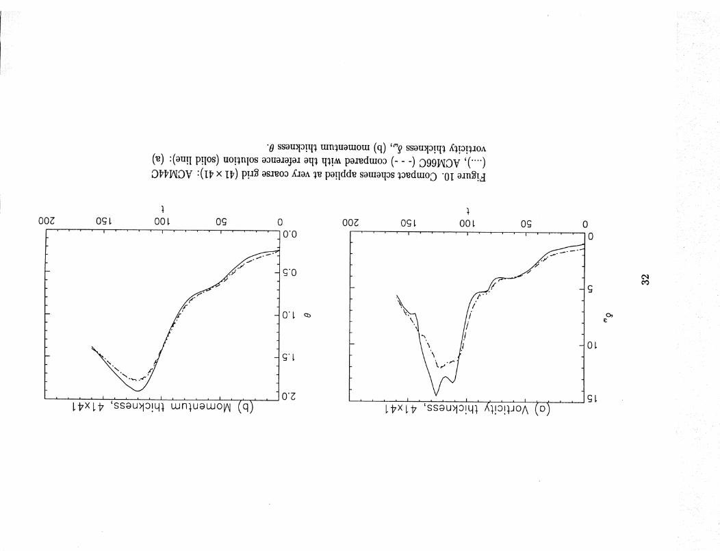
"0 ssou_p!q_ mn_uomom (q) ''_ ssou_p!q_ ,(_p!_:_OA
(_) "(OU!I P!IOS) uoNnlos oouosojoa oq_ q_!,_ poI_3duxoo (- -) 0991AIOV '( .... )
ODITIAIOV "(Ilz x ID) P!_ os:t_o_ daoA _,_ po!idd_ sotuoq_s _,_dmo O "0I oan_!d
l
O_ L O0 L O_ 0
o_°_
°_
m _ I , , I J I , , ,
L ,xL L dowon(;q)
1
ocj L O0 L Og 0' ' ' ' I ' ' ' ' I ' ' ' ' I ' , _--T ......
. " _'" "'_.
i ! L
L_
OL
gL
o?
iii _ •_:_ii!_!':II(I)!_I,:ii_!
:i̧̧ ¸ • )-i/::-.
_i_ ,/__ _iii-)_,:_,:,i_:
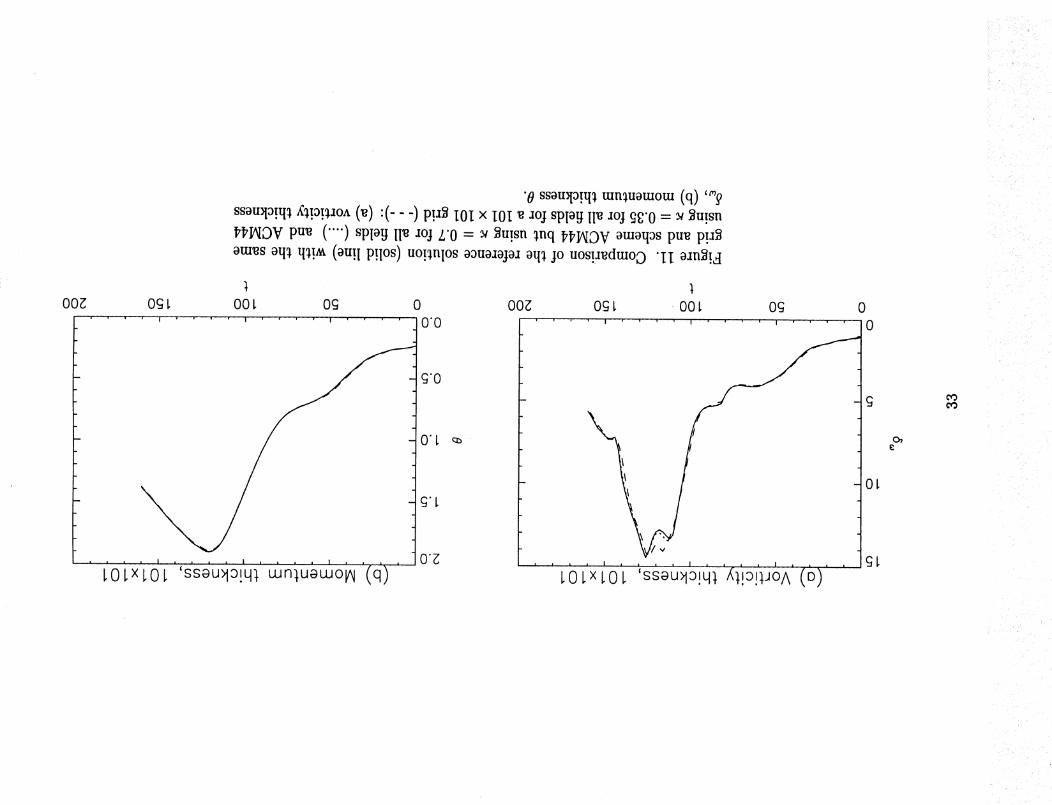
"0 ssomp!q_ mn_uomom (q) ''9
ssomp!q_ _!a!_aOA (_) "(-- -) p!a_ IOI × IOI _ aoj splo U II_ aoj _'0 = u _u!sn
I'I'IAIOV pu_ ( .... ) splog II_ soj Z'O - u _u!sn _nq lzI,_OV otuoqas pu_ p!a_
arrays oq_ q_t._ (ou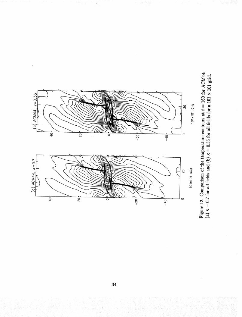
i¸_I_i_i:iiii_iili_i! !il
00 0
I I
('% _-""_-.--/ JJIZ J _. _, _ -_..--%,1 --- - -
0
\
0 0 0
C'q _.-
I I
o
"0°_
t,..ro
o
x
o
t,_
o
x
0
ro.<,-,
x
.,$_ t,.-=
0 _
_ m
r..)_t'.-
34
"0 ssou_p!q_, mn_uomom (q) "_ ssou_p!q_,
A:_t.a!_aoA (_) '(- - -) p!s_ tot x tot aoj spio_t a_ou!i oq_ aoj 0 - u pu_
splog :[_am.lUOU oq_ :[oj L'O = _ _u!sn DD_OV pu_ ( .... ) spl°g IF :[oj ££'0 =
'DDIAIDV oq_, q_t._ (ou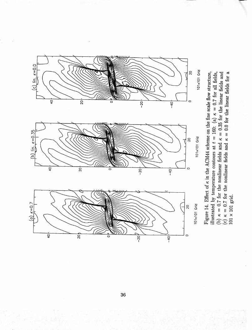
, "_ _ _ . . , . . , .
. •
.._o
o
I I
o o o ' 00 0
I I
II
o o oo o
I I
_ _._00¸
__o _0
o_n.q
_ II _-.0-_¸
"_ O0 0.._ oo •
o _ II II
o _-__==x
"- _ o "_ "_
< o _ ,-.
_J
o_,,i
o .__ ,_ _ ,._0
o _ _ _ _ X
36
; • i_i!iif_ii_i!,Lii_ ¸
o ._
x
x
0
(:3 0 0 E)
I I
37
! i i ¸ i i

:: ..... :i¸ i_ _,:/ • ,:
_: <L:: !(:_ii_ : ;
i!/, _ ii _ _
•(p!a_ I0I x IOI) NzlAIOV oq_ aoj 09I = _ _u ssno_
-uoo osn_aodtuo_ oq_ soj sso_!tu!I xnlj _uoaojj!p 17jo uos!a_dtuo O "9I osn_!d
P!,JO L'_XL'_ P!J9 LOLXLOL P!JO LO_XLO_'
O_ 0 O_ 0 O_ 0
P!J9 I.O_'XI,0_'
O_
017-
0_-
O_
O_
oo
..... ,_ ii,__:_
•;I_ :i
, _ i!_
i_ •
, ii_
ii_ _i_
i i!iii:
iiii _; _i_!ii_iiii_!'
iiiiiill i!!iill _
iiii!!iiiii!ili_iiiiiill
iiiiii!iii:iii!i_i_ii_/i
! i_/¸
ili,i!iii!i!i!!!i!iii̧ ¸
00_
•p!a_ I8 x I i_£
soj H'IAIDV pu_ H'CIAI '(I9I x II,9) uop, nlos oauosajoa (a) pu_ 99I_OV
pu_ i'i'I4IOV 'i_i;IAIOV (q) '99GAI pu_ l'l'GAl 'i_i_GAl (_) :as_ _,s_ s_£v, I
-s_qs-)poqs _q_ aoj OgI = ; _ sano_uo_ £_!su_p jo uos!a_dtuo O "ZI _sn_3
OgL
OOL OgT
0
OOL Og!
, .
OL
:!i I "
K,:, • • • '
!ii, _i _i_,:II:_I_ _:ii
. i :/?_ii:_I:II:_
_.:_ ' ,iil. • i_ _ ,
_,.< _ i_ _,
,!i
• _ _ . _:i/_
: ::/_ ,_i:_:::i:_:,
._ ii_,
ili%
i i!iii!i}_:_
°
(qzI a-m_!d)"_uo o 'ZI aan_!d
og L O0 L og
o
0
i_____ iii:_iiiiii,)ii_i
<,
_i__:_ii} i_i:_:_:ii!.!i
_' ,, '!i_ii_/::,_i__,:,
• ...._ _ii__,_•.....
<,
00_ og L O0 [ OCj 0
' ' ' 0_-
og L O0 L Og
c::>
OL-
01,
O_
OL
T--'t
i_i:__ _/ii_i_i_¸¸/i__
i, . <i i,i' /i i_
• • ,i:__....
_i_/__I,_......:if!_ !_
• • _:i _i__,I_
/ii!!!,i,iiiiilli_ i_ii_!_i_iii
: _iii_ ii_i_:/i_ii'i__
. • ii _ .i _
L
ii
"'°'o°o'_
Lf) 0 Lf_ 0 Lf)
C",I C",l _ .,-- 0
0=,_ ]D d
O=X _o d
0cO
0
0Oq
00 x
0O0
0cO
0
0
o o
o _,.-,o
_N x
oNN
_ ._ _.-_
o _ _o
O m
e_
i
o
o
_ x
o1:21 e_
_ _._
42
• / L, _
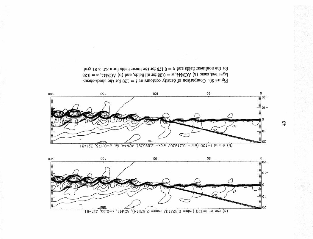
OOE
•p!a_ I8 x I_£ _ so3 spIoU s'eau!i oq_ aoj £LI'0 - _ pu_ sPioU s_OU!lUOUoq_ soj
_£'0 - _ 'DDIAIDV(q)pu_ 'splo!3 IF aoj ££'0 - _ 'NTIAIOV(_) :os_o _so_ ao,_ I
-a_oqs-_poqs oq_ aoj 0gI - _ _ sano_uoa _!suop jo uos!a_du_o D "0g oan_!_
O(::JI. O0 I, OCj 0, , • ' OE-
OL-
OL
O_
¢0
!i_ _ _i_iI_! i_ii i i_. ¸
_i_i ' ,_ _ i: .... _ _
00_
.......... pV_ I8 x l:iSg_ :toj
splog :mau!i oq_ :toj £ZI 0 - u pu_ splog :mOU!lUOUoq_ :toj _g'O - u '£ :toSim!i
'lzlzIAIOV(q) pu_ 'spptj IF _oj ££'0 - u '£ +to+.!tat.['Iz_,lAIOV(_) "os_3 _so_,:to.4:_l
-:moqs-_poqs oq_ _ol OgI - _ _ s:tno_uo_ £_!suap jo uos!:mdmo D 'Ig o:m_!d
og L O0 [ Og| f i
Og L O0 i Og 0
' ' ' 0+-
• _ • _ i_ • _
/
i_i_ ........
i :i_ _
/
i
4
C3
0l-
OL
O_