performance of physics-driven procedural animation of...
TRANSCRIPT

Thesis no: MECS-2015-03
Performance of Physics-Driven
Procedural Animation
of Character Locomotion
For Bipedal and Quadrupedal Gait
Jarl Larsson
Faculty of Computing
Blekinge Institute of Technology
SE�371 79 Karlskrona, Sweden

This thesis is submitted to the Faculty of Computing at Blekinge Institute of Technology
in partial ful�llment of the requirements for the degree of Master of Science in Engineering:
Game and Software Engineering. The thesis is equivalent to 20 weeks of full-time studies.
Contact Information:
Author:Jarl LarssonE-mail: [email protected]
University advisors:Ph.D. Veronica SundstedtPh.D. Martin FredrikssonDepartment of Creative Technologies
Faculty of Computing Internet : www.bth.seBlekinge Institute of Technology Phone : +46 455 38 50 00SE�371 79 Karlskrona, Sweden Fax : +46 455 38 50 57

Abstract
Context. Animation of character locomotion is an important part ofcomputer animation and games. It is a vital aspect in achieving be-lievable behaviour and articulation for virtual characters. For gamesthere is also often a need for supporting real-time reactive behaviourin an animation as a response to direct or indirect user interaction,which have given rise to procedural solutions to generate animation oflocomotion.Objectives. In this thesis the performance aspects for procedurallygenerating animation of locomotion within real-time constraints isevaluated, for bipeds and quadrupeds, and for simulations of sev-eral characters. A general pose-driven feedback algorithm for physics-driven character locomotion is implemented for this purpose.Methods. The execution time of the locomotion algorithm is evalu-ated using an automated experiment process, in which real-time gaitsimulations of incrementing character population count are instanti-ated and measured, for the bipedal and quadrupedal gaits. The sim-ulations are measured for both serial and parallel executions of thelocomotion algorithm.Results. Simulations of up to and including 100 characters are per-formance measured providing an overview of the slowdown rate whenincreasing the character count in the simulations, as well as the per-formance relations between bipeds and quadrupeds.Conclusions. The experiment concludes that the evaluated algo-rithm on its own exhibits a relatively small performance impact thatscales almost linearly for the evaluated population sizes. Due to therelatively low performance impacts it is thus also concluded that for fu-ture experiments a broader measurement of the locomotion algorithmthat includes and compares di�erent physics solvers is of interest.
Keywords: Procedural animation, Interactive games, Multithread-ing, Software performance
i

Acknowledgements
Warm thanks to my family and friends, near and dear; for all your support andencouragement! Big thanks to my supervisors, Veronica Sundstedt and MartinFredriksson, for guiding me through this project. Lastly, a special thanks toMichiel van de Panne for the insightful answers to my questions about procedurallocomotion.
ii

Contents
Abstract i
1 Introduction 1
1.1 Procedural Articulation . . . . . . . . . . . . . . . . . . . . . . . 21.2 Procedural Terrestrial Locomotion . . . . . . . . . . . . . . . . . . 41.3 Problem Statement . . . . . . . . . . . . . . . . . . . . . . . . . . 6
1.3.1 Aims and Objectives . . . . . . . . . . . . . . . . . . . . . 71.4 Research Question . . . . . . . . . . . . . . . . . . . . . . . . . . 81.5 Method Introduction . . . . . . . . . . . . . . . . . . . . . . . . . 81.6 Contribution . . . . . . . . . . . . . . . . . . . . . . . . . . . . . . 81.7 Thesis Outline . . . . . . . . . . . . . . . . . . . . . . . . . . . . . 8
2 Background and Related Work 10
2.1 Locomotion . . . . . . . . . . . . . . . . . . . . . . . . . . . . . . 112.1.1 Believability in Animation . . . . . . . . . . . . . . . . . . 112.1.2 Terrestrial Locomotion Terminology . . . . . . . . . . . . . 11
2.2 Dynamics-Driven Procedural Locomotion . . . . . . . . . . . . . . 122.2.1 Inverted Pendulum Methods . . . . . . . . . . . . . . . . . 142.2.2 Muscle-Driven Methods . . . . . . . . . . . . . . . . . . . 142.2.3 Pose-Driven Feedback Methods . . . . . . . . . . . . . . . 15
2.3 Parallel Execution of Locomotion Algorithm . . . . . . . . . . . . 162.4 Performance in Parallel Algorithms . . . . . . . . . . . . . . . . . 162.5 Summary . . . . . . . . . . . . . . . . . . . . . . . . . . . . . . . 17
3 Implementation 18
3.1 Implemented Algorithm . . . . . . . . . . . . . . . . . . . . . . . 183.1.1 Gait Player . . . . . . . . . . . . . . . . . . . . . . . . . . 213.1.2 Virtual Forces . . . . . . . . . . . . . . . . . . . . . . . . . 213.1.3 Leg Frame and Torque Feedback . . . . . . . . . . . . . . 223.1.4 Legs . . . . . . . . . . . . . . . . . . . . . . . . . . . . . . 233.1.5 Gravity Compensation . . . . . . . . . . . . . . . . . . . . 243.1.6 Foot Placement . . . . . . . . . . . . . . . . . . . . . . . . 253.1.7 Proportional-Derivative Controllers . . . . . . . . . . . . . 26
3.2 Constrained Rigid Bodies using BulletPhysics . . . . . . . . . . . 26
iii

3.3 Optimization . . . . . . . . . . . . . . . . . . . . . . . . . . . . . 263.4 Controller Logic . . . . . . . . . . . . . . . . . . . . . . . . . . . . 283.5 Summary . . . . . . . . . . . . . . . . . . . . . . . . . . . . . . . 30
4 Method 32
4.1 Scenarios and Parameters . . . . . . . . . . . . . . . . . . . . . . 324.2 Technology . . . . . . . . . . . . . . . . . . . . . . . . . . . . . . 354.3 Validity Threats . . . . . . . . . . . . . . . . . . . . . . . . . . . . 364.4 Summary . . . . . . . . . . . . . . . . . . . . . . . . . . . . . . . 37
5 Results 38
5.1 Observations . . . . . . . . . . . . . . . . . . . . . . . . . . . . . . 385.1.1 Measurements . . . . . . . . . . . . . . . . . . . . . . . . . 38
6 Analysis 42
6.1 Serial Results Analysis . . . . . . . . . . . . . . . . . . . . . . . . 426.2 Parallel Results Analysis . . . . . . . . . . . . . . . . . . . . . . . 446.3 Trends and Relations . . . . . . . . . . . . . . . . . . . . . . . . . 446.4 Summary . . . . . . . . . . . . . . . . . . . . . . . . . . . . . . . 46
7 Conclusions and Future Work 48
7.1 Thesis Summary . . . . . . . . . . . . . . . . . . . . . . . . . . . 487.2 Method and Implementation Discussion . . . . . . . . . . . . . . . 497.3 Conclusions . . . . . . . . . . . . . . . . . . . . . . . . . . . . . . 507.4 Contribution and Comparisons . . . . . . . . . . . . . . . . . . . . 517.5 Future Work . . . . . . . . . . . . . . . . . . . . . . . . . . . . . . 51
References 53
iv

Chapter 1
Introduction
Character locomotion is a common subject within the domains of computer ani-mation and games. Locomotion is the description of how propulsive movement isachieved by a body, for animals this translates to the resulting movement patternof their limbs and frames. Terrestrial animal locomotion, more speci�cally, is theway in which an animal self-propel on land by, for example, walking or running.This kind of locomotion and its subsequent animation is common for charactersthat moves around in modern computer games.
Characters in computer games are often displayed as a collection of connectedpolygons and vertices, and thus needs some form of high-level abstracted controllayer to express motions on a per-leg or per-arm level. Animation of polygon basedcharacters in computer games are thus often realized and simpli�ed by means ofmorphing [30,35] or skeletal animation [39]. Both are control techniques used totransform the multitude of vertices of a 3D model, frame-by-frame, in order toanimate it. Both techniques interpolates between keyframes of animation data.
Morphing needs transformed copies of the model for each pose to morph to,while skeletal animation lets the animator control an approximation of the char-acter to be animated. This approximation, a hierarchy of segments, is called askeleton (it can be likened to the common poseable wooden mannequins used byartists). By approximating the character to be animated, the animator will nothave to displace each vertex manually. The segments in the skeleton are referredto as bones. Each bone describes a limb transformation, as a function of time,for the character. Each vertex in the character model belongs to one or severalbones (with weighted priorities) and will follow their transformations. Skeletalanimation and morphing can be combined in various ways as well, depending onthe application.
By using a skeleton, one can thus control separate limbs on a character on ahigh level. Animation of locomotion can then be done on a per-leg basis.
Even though skeletal animation might lessen the amount of parameters to con-trol for transforming and animating character geometry, the full range of motionsexerted by one character alone can become a lot. A computer game featuring arich amount of characters with varying skeleton layouts for animation may thusrequire vast amounts of manual animation work for only various forms of locomo-
1

Chapter 1. Introduction 2
Topic
Transformation Method
Data Generation Method
Articulation Area
Procedural Method
Character Animation
Skeletal Morphing
Procedural Keyframed
LocomotionHead & Eye Reactions
Full Body & Rag Dolls
Grasping & Reaching
Pose Driven Feedback Dynamics
Kinematic & Semi-procedural/Parametric
Musculoskeletal Dynamics
Inverted Pendulum
LeggednessBiped &
QuadrupedOthers (spiders,
insects, etc)
Figure 1.1: Flowchart of domains related to the topic of character animation.Represented as an hierarchical structure, the chart is read from top to bottom andvisualizes the various ways in which a speci�c domain can branch. Domains forleaf nodes to the right are not focused upon in this thesis.
tion alone [21, 39]. When these game characters are expected to work in a largevariety of environments and situations one more or less have to have some form ofprocedural animation component [46]. Not only to alleviate the animators of anexaggerated amount of manual keyframe animation labour, but also to minimizethe memory footprint of the application [39].
Procedural animation solutions can manifest themselves in many di�erentforms depending on the problem and platform. Figure 1.1 presents a hierarchicalview of various domains within the topic of character animation and how thisthesis will present them. Here procedural animation is separated from keyframedanimation. The following section (Section 1.1) will introduce the various com-binable ways a character can express itself through motions; its articulations(Figure 1.1), of which one is locomotion.
1.1 Procedural Articulation
An animated character can express a range of articulations, and the realizationof these are commonly divided into separate solutions. Expressing emotion for

Chapter 1. Introduction 3
(a) Eye articulation (b) Combined articulations.
Figure 1.2: Various forms of articulation used to express emotion and thoughts.In the game The Legend of Zelda: The Wind Waker, eye movement (a) is usedto convey what a character is focusing on. Spore combined procedural and artistmade animations to convey a range of emotions (b).Source: (a) The Legend of Zelda: The Wind Waker: ©2003 Nintendo(b) Spore: ©2008 Maxis (Developer), Electronic Arts (Publisher)
digital characters is a vast problem area [5], and succeeding relies on combiningvarious techniques for conveying thoughts and emotions e�ectively.
Reactive behaviour for characters in form of procedural animation of the headand eyes can be used to convey what a character is currently observing [5] (ortrying to observe), or what it is trying to ignore. Grasping, reaching and loco-motion can be used as a means to achieve or reach a goal. Such intentions canbe made clearer by for example combining it with having the head and eyes looktowards the goal. Examples of character eye movement as well as a combinationof articulation techniques can be seen in Figure 1.2.
The underlying methods to procedurally achieve and animate various formsof articulation overlaps somewhat even though the end usage domains di�er.
In modern games, various layering techniques are often used to combine multi-ple shorter animation clips of skeletal animation together [39], in order to decreasethe total amount of animation data. One example is the Uncharted series by de-veloper Naughty Dog [17, 37]. Various corrective systems might be necessary aswell for repositioning and realigning already animated bones for a character basedon the surrounding environment [20]. Animation systems that changes alreadyexisting animation data to work in a new context, are usually referred to as para-metric [36, 48, 55] or semi procedural [21], see Figure 1.1. These are sometimesreferred to as being kinematic methods.
Within the domain of character articulation for locomotion, semi-proceduralsolutions can be used to avoid locomotion artifacts [59] (such as ill-timed footstrikes or wrongly placed feet) on an already animated character. However, inorder to generate locomotion procedurally from scratch, without already made

Chapter 1. Introduction 4
Articulation
Natural Medium
Means
Gaits
Locomotion
Terrestrial On Water
LeggedCrawling & Slithering
Symmetrical (Walk & Trot)
Assymetrical (Leaping)
In Fluid (Air & Water)
In Solid (Burrow & Digging)
Climbing
Figure 1.3: Flowchart showcasing the various forms of animal locomotion andhow they relate. It describes the context (terrestrial legged locomotion) in whichgaits are used in this thesis. Domains for leaf nodes to the right are not focusedupon in this thesis.
animation data, we need to �rst look at what kind of locomotion is to be gener-ated.
The way in which locomotion is expressed depends on the medium to whichthe characters relies for propulsion (see Figure 1.3). Movement in media, suchas �ight in air, swimming in water or digging through a solid will result in otherenvironmental dependencies and results compared to movement on media. Move-ment on media in turn will di�er for solids and �uids. There exist several meansof propulsion on solids, these can be narrowed down to the use or non-use of legs(see Figure 1.3). Locomotion on a solid is known as terrestrial locomotion.
The following section (Section 1.2) presents the various techniques that existfor generating terrestrial locomotion procedurally without animation data.
1.2 Procedural Terrestrial Locomotion
The game Spore by Maxis presented a delicate animation problem of having toanimate user-created creatures of varying anatomies and skeleton topologies. Itused several kinematic systems that, when combined, would let a legged creaturemove about in uneven terrain, with a procedural animation solution that gener-ated new frames of animation and transformations for bones based on movementvelocities and terrain features [19]. In summation, this system presented onepossible solution for procedurally solving and generating animation for terrestriallocomotion.
The speci�cs of how an animal moves its legs during terrestrial locomotion

Chapter 1. Introduction 5
0 50 1007525
Stance phase Swing phase
Heel strike Mid-stance Toe-offHeel-off Mid-swing Heel strike
Figure 1.4: Gait analysis of human walk cycle, using classical terminology. Thephases are expressed in percentage of the total gait cycle. The �gure is adaptedfrom previously published gait data [56].
in relation to its speed is known as gait [1, p. 14]. Gaits are patterns de�ningthe locomotive cycle needed to an achieve a certain movement speed for a certainanimal.
Gait patterns can be expressed for a varying amount of limbs and styles oflocomotion. An example of a gait analysis of the human walk cycle can be seenin Figure 1.4. In Spore, gait patterns are generated based on the amount of feetand their layout. This pattern then serves as the basis for the overall locomotionanimation [19].
For procedurally animating the gait of a character, there exist several meth-ods, as shown in Figure 1.1. These methods mainly di�er in the amount of dataand computation that are needed to generate the �nal motion. A proceduralkinematics-driven animation system directly manipulates limb positions and an-gles to generate procedural motion. Dynamics-driven solutions, also known asphysics-driven, estimates forces and torques needed for a physics solver to gen-erate the �nal motions. This thesis focuses on physically simulated limbs thatpropels the character forward. In games, character physics can e�ectively be ab-stracted further, regarding a character as just a single rigid body or similar, forlocomotion [47]. Though there are examples of more complex simulation solutionssuch as Euphoria1 by NaturalMotion. Upcoming games (as of writing) such asUncharted 4, are showing a trend towards a more common usage of more complexabstractions, with full body physics combined with motion capture data2.
For the purely procedural methods; dynamics-driven procedural solutions arein general regarded to yield results with more physical realism compared tokinematics-driven pure procedural methods, which tend to su�er from sti�ness inmotion. However, a kinematics-driven animation system has the potential of pro-
1www.naturalmotion.com/, Accessed 2015-01-312www.gameinformer.com/b/features/archive/2015/01/23/
how-uncharted-4-is-taking-game-technology-to-the-next-level.aspx, Accessed 2015-01-31

Chapter 1. Introduction 6
viding a smaller performance impact compared to dynamics-driven methods [22].One dynamics-driven locomotion method is the inverted pendulum [28] model
which abstracts away the knees from the character armature and calculates footplacements to balance the armature approximation. Positions and angles for theknees and feet are then free to be generated either kinematically or solved by aphysics solver [53].
For better biological realism, one can simulate the muscles driving the move-ment of each bone in a character, using musculoskeletal dynamics [57].
Pose-driven dynamics, is a third dynamics-driven option with roots in the�elds of control logic- and robotics theory. In pose-driven methods, each jointis simulated just like in the musculoskeletal methods, but in a simpler fashion,more akin to those of a robot. The simulation tries to achieve precomputed poses,taking physics into consideration.
Feedback mechanisms, such as foot-to-ground collision can be used to furthercontrol a dynamics-driven simulation appropriately.
All these various methods of dynamics-driven procedural animation of loco-motion di�er in resulting visual quality and performance impact. In regardsto performance and in the context of a game with real-time aspects, the needto update a multitude of limbs has the possibility to become computationallyexpensive. Though these dynamics-driven methods are presented as capable ofreal-time simulation, there exists a lack of measurements of how such algorithmsscale performance-wise when simulating multiple characters.
1.3 Problem Statement
The amount of academic research available on the performance impact of dynamics-driven locomotion algorithms is lacking. Though intelligence in this area mightexist internally within the games- and software industry.
Articles presenting dynamics-driven procedural animation methods for loco-motion focuses on the animation quality aspects. Some performance informationis brie�y mentioned for some of these works, to prove that they are able of real-time execution [8, 9, 13,14,27,57].
Another aspect lacking is the performance of said algorithms for more thanone character, although it has been reported as viable within real-time speeds [26,49,51] in single-threaded environments.
For dynamics-driven locomotion algorithms, there thus exist a gap for whatkind of execution times can be expected for such an algorithm for bipeds andquadrupeds, including the performance e�ects of increasing the amount of simu-lated characters.

Chapter 1. Introduction 7
1.3.1 Aims and Objectives
Developing and investigating a solution for procedural animation might provideinsights of its possibilities performance-wise as well as provide a platform forsimulating the locomotive movement of several creatures in games and similarreal-time visualization oriented software, with the possibility of richer environ-ments [34].
Knowledge of performance impact in games is necessary as games needs toexecute in real-time speeds to convey a sense of continuity to the user and nothamper the user's ability to interact with the software [38]. Thus it becomesnecessary to identify what trends can be observed on the performance of a proce-dural locomotion system handling the cyclical feet- and leg movements of groupsof characters, in a game-like setting (in this thesis: an application capable ofrendering the simulated result in 3D, in real-time).
Pose- and feedback-driven real-time simulation methods for locomotion, o�erphysically simulated movement which can respond to external forces, without theneed to simulate full muscle movement. It might thus be a strong contender foran interactive application or game.
The aim of this thesis is to extend the knowledge available for performanceimpact of procedural locomotion algorithms. This thesis will focus on one: apose- and feedback driven algorithm. It will furthermore focus on simulationof bipedal and quadrupedal characters using such an algorithm. As the currentgeneration of PCs and video game consoles (SONY PS4 andMicrosoft Xbox One)provide viable platforms for executing parallel algorithms, the thesis will providean overview of how performance scales between serial- and parallel execution ofthe algorithm as well.
The thesis aims to ful�l the following objectives:
� Implement a pose- and feedback-driven locomotion algorithm for bipeds andquadrupeds, based on existing work.
� Present the performance impact of the implemented pose- and feedback-driven locomotion algorithm.
� Show how the performance of the algorithm is a�ected when increasing theamount of simulated characters.
� Present performance relation between bipedal- and quadrupedal characterssimulated by the algorithm.
� Present performance relation between single-threaded and multi-threadedexecutions of the algorithm.

Chapter 1. Introduction 8
1.4 Research Question
Given a physics-driven procedural locomotion system, which uses a pose- andfeedback-driven simulation method: what real-time performance relation betweena single-threaded and multi-threaded execution of such a system can be observedwhen animating a group of characters; in relation to the population count andthe character leg count?
1.5 Method Introduction
The aims and objectives of this thesis will be realized through an experiment.The experiment consists of several executions of the implemented locomotionalgorithm, in which the execution time of the algorithm is measured. The exper-iment will increment the character count for each measurement. Measurementswill be performed on both bipeds and quadrupeds, separately. Measurements areseparately performed on both serial- and a parallel executions of the algorithm.The experiment is further described in Chapter 4. By doing an experiment whichsystematically measures and records the performance results, comparison graphscan be generated for the objectives.
Another possible method, which was not chosen for this thesis, is for examplea user case study of visual quality of the generated result. Instead, an alreadyvisual quality tested algorithm (using closeness to motion capture data) was im-plemented (see Section 1.6) for focus on run-time performance evaluation.
1.6 Contribution
This thesis presents a novel standalone implementation of a pose- and feedback-driven locomotion system. It is based upon the previous work on locomotionalgorithms by Coros et al. [8, 9] and Yin et al. [60]. It di�ers from previousalgorithms in that it relies on BulletPhysics for solving the generated torques,it supports both serial- and parallel execution and it supports both bipeds andquadrupeds (with a �exible spine for quadrupeds) using the same algorithm.It furthermore presents performance measurements of the algorithm for varyingamounts of characters, for both serial and parallel execution. Figure 1.5 presentsa screenshot from the �nished application and the resulting simulation of thelocomotion algorithm implemented.
1.7 Thesis Outline
Following this introduction is Chapter 2, Background and Related Work, whichprovides an analysis of existing literature within the domains touched upon by

Chapter 1. Introduction 9
Figure 1.5: Screenshot of the application developed for the thesis. It shows walk-ing bipeds and quadrupeds, simulated using the implemented pose-driven feedbacklocomotion algorithm. In this screenshot an example of interactivity is shown byhaving boxes thrown at the characters to disrupt their balance.
this work. It starts with an introduction on what have in�uenced the develop-ment of various procedural methods of animation, with focus on locomotion, aswell as descriptions on terminology. The dynamics-driven procedural methodsfor locomotion mentioned in this chapter are described further. Chapter 2 alsoprovides more insight and introduction to speci�c terms in the surrounding areaswhich contribute to the basis of this work, such as animation-, locomotion- andparallelism theory.
This is then followed by Chapter 3, Implementation, which introduces themodel of choice for the procedural animation itself and its components, as wellas supporting components and measuring methods in the �nished application.
Chapter 4, Method, describes the method and settings for performing theexperiment. Chapter 5, Results, then presents the following observed results. Ananalysis of the results, showing the rate of change when increasing the amount ofcharacters, is presented in Chapter 6, Analysis.
Chapter 7, Conclusions and Future work, concludes the thesis and providesdiscussions on the experiment, the experiment results and the locomotion algo-rithm implementation.

Chapter 2
Background and Related Work
There is an absence of available research on performance of procedural animationof locomotion for serial and parallel multi-character simulations using dynamics-driven techniques. This is likely due to the fact that there is still a lot of ongoingresearch in �nding more robust and visually pleasing simulations [13,44]. Pronostet al. brie�y mention a 4 × real-time performance for a, presumably serial,dynamics-driven animation system [44]. Coros et al. report a performance of10× slower than real-time for 16 physically simulated characters [8]. Fang et al.reports real-time results [11] for their kinematic- and dynamics-driven animationsystem of myriapoda. Geijtenbeek et al. mentions their simulation having highperformance [14] and being able to simulate in real-time. Johansen providedsome real-time performance measurements and hardware speci�cations for hiskinematic parametric locomotion system [21].
Modern interactive software and games are running in environments whichsupports multi-threaded applications. There is thus an opportunity to investigateperformance variances and relations between parallel and non-parallel executionsof an algorithm.
There exists a large amount of research on various forms of techniques forprocedural animation of locomotion [8,9,13,19,21,25]. Especially the number ofpublished research on physics-based procedural animation has been showing anincreasing trend [13, p. 11].
All of this, as well as the pure aesthetic aspects that exist within games as amedium will impact the choice of algorithm model for procedural animation. Inregards to developer usability, one should also take into consideration the harmthat too much complexity or too little control might have on the developmentpipeline for artists and programmers.
This chapter begins with establishing a common understanding of domainspeci�c terminology that will be used throughout this thesis. This is done by �rstproviding a short introduction on the various aspects of animation quality and theexisting ideas for this �eld and how they, in di�erent ways, have in�uenced earlierworks of procedural animation. Following this are explanations of terminologyused to describe various aspects of locomotion which are commonly used withinthe �elds of biology, robotics and animation.
10
Chapter 2. Background and Related Work 11
After these introductory sections on terminology, an analysis of existing workson di�erent procedures of procedural animation is presented, along with theirreported properties in regards to result, implementation data and functionality.In the concluding part of this chapter a brief review of existing paradigms forparallel programming are presented as a foundation for the parallel execution ofthe implemented locomotion algorithm.
2.1 Locomotion
As mentioned in Chapter 1, locomotion is but one aspect of character articulation.It can be used to provide one part of the puzzle to construct believable virtualcharacters.
2.1.1 Believability in Animation
When discussing the quality aspect of animation of virtual characters, one needto make a distinction between believability and realism. In order for a personto perceive a virtual character as believable it does not necessarily need to berealistic [42]. Believability is sought after in interactive applications containingvirtual worlds and characters in order to create an engaging experience for theuser [41]. Believability is often achieved by a combination of several expressivebehaviours and by being able to react to events and interactions accordingly [5].Bates et al. conducted surveys using procedural animation of exaggerated emo-tions on cartoon characters in order to see on what level the users connected withthe characters [5]. By combining several forms of character articulations one canthus increase the chances of creating believable virtual characters. Locomotion,being one form of articulation for movement is thus one important part in orderto realize this. One example is the work done by Unuma et al. [54], in whichvarious forms of gait were used in combination with full body poses to conveyamount of exhaustion in a character.
2.1.2 Terrestrial Locomotion Terminology
A single gait cycle for a character contains several step cycles for each of thecharacter's feet. A step cycle is described by its duty factor and step triggerparameters [1, 19]. The duty factor is the percentage of ground contact of thefoot in regards to the whole cycle and the step trigger is the o�set from which afoot's cycle starts. The time in which the leg is in the air is referred to in thisthesis as the swing phase, while its time on the ground is referred to as the stancephase. Figure 2.1 shows a visualization of various gait cycles.
To di�erentiate between various movements within the reference frame of thecharacter, they are categorized by the planes in which they exert movement.

Chapter 2. Background and Related Work 12
Figure 2.1: Gait cycles, de�ning the phase shifts and duty factors. Here pre-sented in percentages of total cycle time. The left notations represents the left-and right legs, with numbering going from front- to back. The stance phases arerepresented as the colored bars, while the swing phases are shown as light-greybars. The graphs are adapted from previously published gait data [4,6,56].
The sagittal plane is the plane which vertically spans from the rear to the front,e�ectively creating the character's left- and right hand sides. The coronal planeis the vertical plane which divides between the front and back of the character.Lastly, the transverse plane is the horizontal plane which de�nes the top andbottom of the character. These planes are shown in Figure 2.2.
2.2 Dynamics-Driven Procedural Locomotion
Dynamics driven procedural animation uses a physics solver of some kind togenerate the �nal articulated angles and positions for the limbs of a character.The means of which the torques and forces are calculated for the solver to applymay wary. Where kinematic solutions use inverse kinematics to �nd the anglesfor intermediate joints for the extremities, the dynamics-based equivalent is aninverse dynamics calculation to �nd the correct torques and forces to perform awanted motion for the extremities to reach their end targets.
Full inverse dynamics are exceedingly computation heavy. They are not, as ofyet, a realistic approach for real-time applications [44,58]. Instead of full inversedynamics, various forms of approximations are used, of which each are specializedfor a certain type of articulation. Such specialized approximated methods will

Chapter 2. Background and Related Work 13
Coronal Plane
Sagittal Plane
Transverse Plane
Figure 2.2: The planes used as reference frames to express movement in the localspace of a character.
also commonly rely on character speci�c input parameters. In order to �nd thesecharacter speci�c parameters there is often a need for some sort of optimization [1,pp. 10-12] phase to �nd a set of parameters that result in a robust gait [9,14,44,57],though some models manages to avoid it [8, 25].
Gait optimization phases are used to teach a character with an animationmodel to walk. This is done by ever so slightly change a set of input parametersfor the model and the character, and test the result for each change [9]. Onemethod of �nding an optima of parameters is by letting the result be graded bya set of wanted criteria, and perform some form of greedy selection [31]. KarlSims [50] introduced the concept of virtual critters that, through simulation ofevolution, could learn how to propel themselves in their virtual environments. Hismodel simulated several generations of critters. In this model, the most successfulcritters where allowed to evolve and change behaviour and shape.
For procedurally animating the locomotion of a character for a physics solver,there exist three major types of methods, with focus on real-time animation forgames and interactive simulations, for which the majority of academic researchhas been made. The following sections (Section 2.2.1, 2.2.2 and 2.2.3) outlinethese and how they di�er from- and relate to each other.

Chapter 2. Background and Related Work 14
2.2.1 Inverted Pendulum Methods
The Inverted Pendulum (IP) model [24, 28, 45, 53] has been used as a way for�nding foot placement for balancing dynamics-driven characters. The swing-ing motion apparent in the movement of the legs in bipeds have shown to beachievable by approximating the legs with an inverted pendulum [29]. The in-verted pendulum model does this approximation by neglecting the knees. Full legmovement can then for example be provided kinematically upon the solved footplacements by the use of inverse kinematics.
The balancing of quadruped characters can also be approximated by the IP-model, this by utilising two pendulums; one for each pair of legs [1,15]. Kenwrightbuilds upon the model for bipeds to make it able to generate more aestheticallypleasing result [25]. This by for example introducing the use of an elongated bodyrepresentation instead of a single point as well as impulses, to better visualizewalking on uneven terrain and to get more dynamic results.
The model for humanoid bipeds can also be expanded by using a spring-damper setup for each leg, as these act as an acceptable approximation of thehuman muscles [23]. The inverse pendulum model can be used as an externalfoot placement model for other dynamics-driven locomotion solutions [8].
2.2.2 Muscle-Driven Methods
Dynamics-driven methods may generate motion parameters by simulation of mus-cles. Though it generally adds additional layers of complexity compared to othermethods, it is regarded to achieve the most realistic results. As the strength andenergy expenditure of these virtual muscles may be altered, they prove useful ininteractive medical simulations [57].
Wang et al. presented a solution for procedural locomotion using a Muscu-loskeletal driven dynamics model [57]. It used a virtualHill-type muscle model [14,57] to apply biologically constrained forces upon the limbs. An o�-line optimiza-tion phase using biologically based �tness functions, such as the amount of e�ortneeded by the model [57], was used to �ne-tune the gait parameters driving themodel in order to achieve realistic movement and allow for simulation of variousmuscle de�ciencies.
Geijtenbeek et al. improved on this method by introducing an o�-line opti-mization phase that routed muscles along the skeletal hierarchy automatically [14].This method lessened the need for biologically correct muscle data during con-struction of the character model. It further allowed for the creation of virtualcreatures with �tting gaits based on their anatomy. Creatures with more unreal-istic proportions thus evolved gaits to compensate.

Chapter 2. Background and Related Work 15
2.2.3 Pose-Driven Feedback Methods
Dynamics-driven movement can also be generated from a set of kinematic tar-gets [13]. Motion graphs of kinematic animation data contain the wanted tra-jectories that the physics model should follow as best as it possibly can. Thismodel further relies on concepts common in the �elds of robot- and control logicto allow for the characters to achieve the prede�ned movement from the graphsas close as possible. Feedback Proportionate Derivative (PD) controllers are usedto generate variable torques on each joint in order to match the motion graphs.
It is worth noting that in PD-controllers an additional integral term can beimplemented as well to eliminate steady state errors (di�erence in the set goal andthe actual steady state of the controller). This type of controller is then known asa PID-controller. This is however of limited use for character animation [13, p. 32],where the goal is often constantly changed (as it is being animated).
Raibert et al. developed early robotics inspired models for dynamics-drivenbiped- and quadruped gaits [45]. SIMBICON [60] by Yin et al. built upon severalof these early concepts to produce stable biped gaits that could learn from a setof artist created key frames. This model was optimized to withstand pushes,without falling, to some degree. It has since then been further expanded on-, orinspired methods similar to it to support a wider arrange of biped actions [36] andquadruped gaits such as galloping [9]. The use of virtual forces, another conceptfrom the �eld of robotics [40,43,52], have been used in some models [8,9] in orderto compensate for gravity and allow for lower PD-gains, in turn allowing for lesssti� movements.
The motion graphs used for animation can be created by an animator (askey-frame data) or by using mathematical functions. Motion graphs can also beextracted from motion capture recordings. This motion graph data, along withthe control system parameters and PD-gains are then generally subjected to someform of optimization as well.
Compared to the musculoskeletal driven models, the graph driven modelsmight result in less realistic movements. However, as it conforms to the wantedmovement solution for a character rather than �nding the optimal movementsolution based on anatomy, it might leave more room for artistic freedom andthus be more usable in games.
The optimizations needed for many dynamics-driven methods may use motioncapture data or rules on acceleration, velocity and amount of rotation. Severaliterations are executed, each with a new perturbation on dependent parameters.Fitness for a set of parameters in an iteration is evaluated to allow the model to�nd its optimal parameters for how to move and balance [9,14,36,57]. Some localoptimization techniques that have been used for locomotion controllers includesfor example stochastic greedy algorithms [9,31] and covariance matrix adaptation[36, 44].
The implemented algorithm in this thesis (which will be measured in the

Chapter 2. Background and Related Work 16
experiment) was chosen to be a graph-, virtual force- and PD driven model (ef-fectively a pose-driven feedback model) as described by Coros et al. [9]. Somein�uences were also taken from two similar solutions presented by Coros et al. [8]and Yin et al. [60]. The implementation done for this thesis is further describedin Chapter 3.
2.3 Parallel Execution of Locomotion Algorithm
There is a possibility that character animation in a game will be executed forseveral characters. As a serial implementation of an algorithm grows in size, itmight become relevant to investigate whether it lends itself to parallelization ornot.
The animation methods presented in Section 2.2 all contain somewhat ex-ploitable phases of various levels of data parallelism. Data parallelism is possiblewhen each processing unit in a system can execute the same instruction set onseveral data sets.
Data parallelism contrasts to task parallelism which might execute di�eringinstruction sets over threads. Data parallel components are well suited for paral-lel execution due to their inherent independence from component-to-componentcommunication (which might require synchronization). A data parallel approachto algorithms for execution are one important quirk [12] to SIMD-like (Single In-struction Multiple Data) architectures as they perform poorly when experiencingtoo many branching instructions.
Even though the architecture of modern CPUs are better suited for codewith branching patterns compared to SIMD architectures, they also do have thepossibility to bene�t from data parallel algorithms [32].
2.4 Performance in Parallel Algorithms
Amdahl's law [2] and Gustafson's law [16] tell what changes in performance canbe expected when executing an algorithm in parallel. Both of these laws are the-oretical in nature and does not consider the multitude of bottlenecks that occurswhen implementing a parallel algorithm. They do however pose two interestingoutset views of how one can approach parallelization. Amdahl's law states thatthe problem size of an algorithm is constant, and shows how the e�ect of a paral-lelization of an algorithm with fractional possibility of parallelization, results in asteadily declining performance gain as one increases the computation capability.
Gustafson's law, on the other hand, disputes this as the only scenario andclaims that in some cases it is more likely that a large problem set is to be solvedwithin a certain time limit, and thus, the problem size is increased along with thecomputational power, while the time limit remains constant.

Chapter 2. Background and Related Work 17
An algorithm of data-parallel nature may be parallelized on the CPU usingclassic parallel transform features of libraries such as OpenMP, Parallel PatternsLibrary or Intel Threading Building Blocks. These methods are simple to imple-ment for an existing single threaded algorithm, provided all instances of it can beexecuted at once, without the need to wait for each other.
The parallelization of the locomotion algorithm will be done on the per-character level, in order to keep the design of the single- and multi-threadedvariant of the algorithm as close to each other as possible. The number of per-character algorithm executions to be done in serial per parallel invocation isdescribed in Chapter 4. Further described in Chapter 4 is the choice of time limitto be used for the experiment.
2.5 Summary
The �rst part of this chapter provided a review on existing research on the subjectof procedural animation of character locomotion following. Also presented was abrief overview on various quality aspects of animation with respect to believabilityfor richer user experiences in games and interactive software. It also brought forththe various sub categories of procedural animation as well as a closer look on theexisting methods of realising locomotion procedurally. Following this was a briefoverview of the various aspects of parallelism.
In Chapter 3 a motivation for the choice of locomotion algorithm is presented.This is followed by descriptions of the various phases and components present inthe chosen algorithm. It also presents the chosen solutions for parallelism of thealgorithm as well as descriptions of the overlying framework and the methods ofperformance measurement.

Chapter 3
Implementation
In Chapter 2 locomotion terminology was introduced for virtual simulations ofterrestrial locomotion.
As the experiments outlined in Chapter 4 only aim to evaluate performancerelations for an animation model and not its resulting visual quality, considerationneeds to be taken for the choice of animation model with regards to its reported�ndings on visual quality.
Other aspects of importance for choice of model, that are also somewhat basedon existing work, are the level of complexity introduced to the user (or developer)and the availability of control presented. Worth noting as well is that the domainof games might not always favour realism, but rather believability in a certainsetting, as well as artistic freedom.
This chapter begins with a summary and description of the chosen model forprocedural animation of locomotion, along with a motivation with considerationto the domain. This is followed by separate descriptions of the various componentsand phases present in the model, as well as their interactions. The chapter isconcluded with an overview of the interactions of the stages of the model.
3.1 Implemented Algorithm
The implementation algorithm chosen for the procedural generation of terrestriallocomotion, is a dynamics-driven model.
As mentioned in Chapter 2, dynamics-driven locomotion calculates the torquesand forces needed for a physics solver to generate the �nal character motions. Abig aspect of why a dynamics-driven model is favoured instead of a kinematics-driven model, is due to a physics engine's tendency to convey more physically re-alistic movements [13,22], although not necessarily biomechanically accurate [13].The dynamics driven model chosen is a pose-driven feedback model and has itsroots in the SIMBICON algorithm for dynamics-driven locomotion of bipedalcharacters.
Speci�cally, the implementation outlined in this chapter is based on the con-cepts presented by Coros et al. [8, 9] and Yin et al. [60]. It is not built uponthe code bases of these former works, it is a standalone implementation. The
18

Chapter 3. Implementation 19
implemented model di�ers from existing methods in the way that it as a singlemodel supports both bipeds and quadrupeds.
The main aspects of driving the internal articulation of a leg using PD-controllers and virtual forces is carried over to this solution, as is all the steps re-garding the animation of the leg and leg frames. Animation for head, neck and tailhas not been implemented for this thesis. A novel aspect of the implementationfor this thesis is the execution of locomotion for both bipedal and quadrupedalcharacters using the same algorithm, for both single- and multi threaded execu-tion. A data driven paradigm is used where data is separated from logic to allowfor simple data parallel [10] execution.
A pose driven feedback dynamic method was decided upon as it promisessome artistic freedom as the motions can be somewhat controlled by the motiongraphs (the motion trajectory over time) for which the legs and feet tries to matchtheir cyclical movements [8,44,60]. This kind of method also integrates well withcommon physics engines for games, with the promise of a lower performanceimpact [44]. It also promises a possibility for a larger amount of possible gaitscompared to the basic implementations of inverted pendulum models [60].
One drawback when relying on PD controllers for joint control is the addedcomplexity of manual tuning of gains required [53], though this can be alleviatedsomewhat by automatic scaling based on proportions [8]. For this implementa-tion, the gains were manually tuned.
Muscle-based dynamics simulation has proven to more e�ectively generate re-alistic movement [14], but it was not chosen as it adds an extra layer of complexityfor creating- and especially for optimizing characters for simulation.
Multi-threading was implemented using the parallel-for paradigm for non-intrusive implementation of data parallel execution. Both the Parallel PatternsLibrary by Microsoft as well as OpenMP was implemented for this application.For the experiment OpenMP was used, being the more cross-platform alternative.
The full articulated armature that is handled by the physics engine can beseen in Figure 3.1. The overall control loop [9], or controller ; acts on a simpli�edabstraction of the armature, see Figure 3.2. This makes the controller somewhatindependent from the anatomy of the skeleton [9], such as the amount of joints ina leg. Thus the same controller logic can be used for both bipeds and quadrupeds,of various sizes.
A pair of legs of a character are attached to a leg frame, which acts as the localcoordinate system for that pair of legs [9]. A quadruped has two leg frames, onefront leg frame and one back leg frame, while bipeds have one. The leg framesof a quadruped are connected by a chain of joints acting as the spine. The legframe tries to follow a prede�ned rotational trajectory by providing a feedbackof the torque back through the legs in stance.
The physics solver will then interpret the skeleton as a series of connectedjoints with various torques to be applied. Each leg will apply di�erent torques

Chapter 3. Implementation 20
Leg Frame
(a) Biped
Rear Leg Frame
Front Leg Frame
Spine
(b) Quadruped
Figure 3.1: Controller layout as a collection of rigid bodies with joints as seenby the physics engine. The leg frame is here treated as a single rigid body in thebiped (a), while the the quadruped has two connected leg frame rigid bodies (b).The quadruped uses a spine made up of an array of connected rigid bodies withjoints to connect the both leg frames.
Leg Frame
(a) Biped
Rear Leg Frame
Front Leg Frame
(b) Quadruped
Figure 3.2: Controller abstractions for generating propelling motion. Thesesimpli�ed models are what the controller uses to generate the overall motion in-structions, which are then handled in �ner detail by various sub systems. The legframes acts as the local reference frame for the simpli�ed legs and aims to followa prede�ned trajectory. The biped (a) make use of a single leg frame, while thequadruped (b) has one for the front- as well as the rear. Note that at this stage,the number of joints are not taken into consideration.

Chapter 3. Implementation 21
depending if it is in a stance- or swing phase in its animation. A stance leg triesto accomplish the torque needed to keep the leg frame stable. The angle of theknees are calculated using inverse kinematics that de�nes a goal angle for which aPD driver estimates the torque. The feet tries to reach prede�ned lift- and strikeangles.
Following are descriptions for the various stages of the model and their im-portance. The interaction between these stages are then presented in Section 3.4.
3.1.1 Gait Player
The gait player can be seen as the overlying animation player, which incrementthe normalized gait phase Φ = t/T , where t is the current gait time and T isthe total gait period. The progress, φ, in swing and step phase for the legs arede�ned by the step triggers and duty factors of the legs, as well as early or latefoot strikes (when the physics engine registers a foot strike before or after themodel determined it to happen). An early foot strike will immediately force thecurrent phase from swing to stance if φ > 0.8 in the swing phase. A late footstrike triggers a temporary downwards o�set to the foot target position.
3.1.2 Virtual Forces
In order for the abstracted model to be viable, the model takes use of virtualforces [9]. Virtual forces are a form of virtual control method which serves asa means to be able to control general motions in detail while at the same timebe able to exert corrective torques and forces to allow for these motions in anunknown environment [43,52].
A virtual force is expressed as the force we want a certain limb or leg frame totry to achieve, even though this limb might be more complex than the leg vectorfor which the motion is controlled. This force is achieved by translating the forcevector to a set of torques. Figure 3.3 shows the resulting torques for the chain ofjoints in the a�ected limb. Following is the method for calculating torque froma virtual force applied to an end e�ector, as described by Coros et al. [9] andGeiijtenbeek [13].
In order to make the full limb exert the wanted virtual force, the Jacobiantranspose is used for each degree of freedom (DOF) in the limb in order to ap-proximate the sets of torques, τF , for each joint which will amount to the wantedforce as applied on the whole limb (3.1).
τF = J(p)TF (3.1)
The Jacobian Transpose matrix (3.2) is composed of rows, each de�ning therate of change for a point p around a chain link's DOF, αi as expressed as thenormalized axis of rotation in world frame coordinates [13, 44]. The number of

Chapter 3. Implementation 22
Base
VFEnd effector
Figure 3.3: A virtual force applied to an end e�ector resulting in a set of torquesfor the joints in the limb.
rows, k, equal the total DOF count in a chain. Thus, for example; a 3-DOF jointequals three rows in the matrix (3.2).
J(p)T =
∂px∂α1
∂py∂α1
∂pz∂α1
......
...∂px∂αk
∂py∂αk
∂pz∂αk
(3.2)
For each DOF i in a chain, the virtual force F is thus transformed resulting inthe torque exerted by that joint for that force (3.3). Note that this is only a partof the �nal torque. All torques generated by the control loop are summed beforestepping the physics solver.
τF,i = (αi × (p− bi))TF (3.3)
3.1.3 Leg Frame and Torque Feedback
The leg frame exerts the torque τleg frame (3.4). The desired torque for a leg frame,τdleg frame, is calculated using a PD-controller working towards an orientation asde�ned by a motion graph.
τleg frame = τstancelegs + τswing legs + τspine (3.4)

Chapter 3. Implementation 23
-Fv
-Fh -FDi
Fv
FhFDi
Figure 3.4: The virtual forces acting on a leg frame through a stance leg. Theopposite of the forces are applied on the stance foot with the leg frame as basepoint.
The leg frame then works to achieve this torque τdleg frame by feedback to thestance legs (3.5). The torque τstance legs is split evenly among the legs in stance. Itis the �nalized torque for the stance legs, which is supplied to the physics solver.
τstance legs = τdleg frame − τswing legs − τspine (3.5)
3.1.4 Legs
Virtual forces act on the leg frames through the legs which are in stance. Thecalculation of virtual forces assumes a stable base point in order to give goodapproximations. Coros et al. argue that the proportionally larger mass of theleg frame makes it more viable as a base point rather than the feet [9]. The signof the summed leg frame force is �ipped and this resulting opposite force is thenapplied on the stance feet as end point, with the leg frame as base. Following arethe forces exerted upon the stance legs and their leg frame.
A force Fh is applied to the feet to regulate the height of the leg frame basedon a PD controller working from a motion graph. A virtual force Fv (3.6) on thefeet is used to regulate the velocity of the leg frame, where Kv is an optimizedgain factor, vd is the desired velocity and v is the current velocity. The velocityparameters of Fv are further discussed in Section 3.1.6.
Fv = Kv ∗ (vd − v) (3.6)
Chapter 3. Implementation 24
A phase dependent force FD(D) is applied to each stance leg, where D is theamount of forward internal progress of the foot with the leg frame as referenceframe (3.7). Figure 3.4 showcases the forces that acts upon a leg frame througha stance leg.
D = |−→P leg frame −
−→P foot| (projected to ground plane) (3.7)
The constant parameters of FD(D) (3.8) are de�ned through optimization. Thisforce allows for �ne detail tweaking of the motion of each leg [9].
FD(D)vertical = c0 + c1 ∗DFD(D)horizontal = c2 + c3 ∗D
(3.8)
These forces mentioned are not in e�ect on the leg frame if there are no legsin stance.
For the swing legs, a virtual force Fsw is applied to allow for lower PD-gains.Lower PD-gains result in less sti� movements. Fsw uses a PD controller with avariable proportional gain kft(φ) based on an optimized graph.
This PD-controller drives the foot from its current position to its strike posi-tion. The derivative gain is set to ten percent of the proportional gain. Note thatthis solution for Fsw di�ers from the use of a spring-damper solution by Coros etal. [9].
The virtual forces does not guarantee correct placement of the knees. Toalleviate this a two-link inverse kinematics solution, using the law of cosines, isused to calculate the correct knee position (based on the hip- and foot positions).PD-controllers in the joints are then used to calculate additional torque for theleg joints in order to reach the wanted internal joint angles.
3.1.5 Gravity Compensation
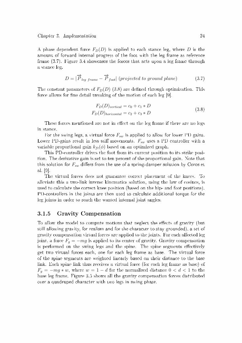
To allow the model to compute motions that neglect the e�ects of gravity (butstill allowing gravity, for realism and for the character to stay grounded), a set ofgravity compensation virtual forces are applied to the joints. For each a�ected legjoint, a force Fg = −mg is applied to its center of gravity. Gravity compensationis performed on the swing legs and the spine. The spine segments e�ectivelyget two virtual forces each, one for each leg frame as base. The virtual forceof the spine segments are weighted linearly based on their distance to the baselink. Each spine link thus receives a virtual force (for each leg frame as base) ofFg = −mg ∗ w, where w = 1 − d for the normalized distance 0 < d < 1 to thebase leg frame. Figure 3.5 shows all the gravity compensation forces distributedover a quadruped character with two legs in swing phase.

Chapter 3. Implementation 25
BaseBase
Figure 3.5: The composition of gravity compensation forces applied to aquadruped character. The forces are applied to swing-phase legs and spine links.Note that each of these forces will result in fractional torques for the precedingjoints of the end e�ector where the force was applied.
3.1.6 Foot Placement
Desirable foot placement, for which the controller strives to achieve is velocitybased. From the foot's current placement P0 a new velocity scaled target positionP1 is calculated as P1 = Pleg frame + (v − vd)s. Where Plegframe is the new, non-scaled, world space foot position as de�ned by a motion graph and o�set by theleg frame's current position. This position is then further o�set by the scaleddi�erence between the current velocity v and the desired velocity vd.
The trajectory for the foot between P0 and P1 follows an optimized step heightpath hsw(φ) in the sagittal plane, where φ is the current progress of the phase. Anoptimized easing graph tsw(φ) furthermore enables variable horizontal movementspeed for the foot.
The desired velocity vd is a value that incrementally tries to reach the userde�ned goal gait velocity. It is the current velocity, incremented or decrementedby a maximum value per second (each frame) until it reaches the goal velocity.
The foot angle in the sagittal plane, is based on the transitions between theswing- and stance phases of the leg. The foot is driven by a PD controller to theprede�ned and optimized take-o�- and strike angles that occur in the transitions.Time o�set parameters for when to switch between target angles are tweaked inthe optimization phase as well.

Chapter 3. Implementation 26
3.1.7 Proportional-Derivative Controllers
The internal shape of the legs, as well as the foot angle and the spine shapeare controlled using PD-controllers. A PD-controller is a feedback reliant meansto minimize a general error value. This error can for example be a di�erencebetween a wanted and a current angle of a joint. A partial torque for a joint inthe character armature can thus be estimated using a PD controller (3.9).
f(t) = Kpe(t) +Kdd
dte(t) where t=time and e=error (3.9)
The gains KP and KD are application dependent as is the interpretation of theresult value f(t). For joint torque control, the result value is directly applied aspartial torque.
3.2 Constrained Rigid Bodies using BulletPhysics
The physics library Bullet Physics, by Erwin Coumans, was used for the physicssimulation. It was chosen as it is an open source engine with constraint support. Itsupports 6-DOF generic constraints which is useful when having constraints withvariable DOFs. Bullet Physics is used in a variety of interactive applications andgames. Parts of Bullet Physics was developed in co-operation with video gamedeveloper and publisher Rockstar Games and integrated in their game engineRAGE , which in turn powers Grand Theft Auto IV, Grand Theft Auto V andRed Dead Redemption1, amongst others. Bullet Physics has also been used invarious movies such as Shrek 4, How To Train your Dragon and Megamind2
Bullet Physics has been deemed to be one of the best performing open sourcealternatives for physics engines [7].
For all simulations in this implementation, Bullet Physics was executed at arate of 120Hz.
3.3 Optimization
An o�-line optimization phase was run for both the biped and quadruped charac-ter to tweak the default parameters (presented in Section 3.1) de�ning the variousrun-time timings and motion graphs. The optimization was done using a greedystochastic local optimization method, as presented by Coros et al. [9]. A greedystochastic algorithm extends a general greedy algorithm by introducing randomperturbations [31].
The optimization only needs to be done once per character. Once the pa-rameters are found, they are saved to disk and used for all other executions of
1www.bulletphysics.org/Bullet/phpBB3/viewtopic.php?p=11971, Accessed 2014-11-092www.bulletphysics.org/wordpress/?p=241, Accessed 2014-11-09

Chapter 3. Implementation 27
1 2
3 4
Figure 3.6: Learning to walk. The images, appearing in chronological order, areshowing iteration stages in the optimization phase. A number of variations of theprevious winning parameter set is tested each iteration and evaluated.
that character. The characters that were simulated in the experiment used suchoptimized parameters to ensure that they walked. An example of the resultingimprovement from optimization of the walking gait for the biped can be seen inFigure 3.6.
The parameter tweaked per controller was the gait period time. The param-eters tweaked per leg frame were: desired orientation graph, desired leg frameheight graph, foot tracking gain graph, desired step height graph hsw, foot swingtransition easing graph tsw, Fh PD-gains, Fv scaling-gain Kv, the constant pa-rameters of FD(D), the foot take-o� angle, the foot strike angle, the scaling factors for foot placement and the step lengths in the transverse plane.
Each graph was represented as a piecewise linear function with 4 single preci-sion �oat data points each (linearly interpolated when read).
The parameters tweaked per leg were: the step trigger, the duty factor, thefoot take-o� time and the foot strike time.
fobj(P ) = wdfd + wvfv + whfa + wrfr (3.10)
A greedy stochastic algorithm aims to minimize the result of a function bychanging the parameters set to be tweaked. The function to be minimized (3.10),fobj is composited of several weighted measurements on the character gait per-formance. Based on these rules a gait resulting from a certain set of perturbedparameters is graded. This evaluation is repeated several times, and each time anew best grade is recorded, the old parameter set is discarded and the followingperturbation is based on those of the current best.
The component fd measures motion deviation. Here Coros et al. used a

Chapter 3. Implementation 28
motion recording of a real dog during various gaits. As motion capture data wasnot available as a part of the implementation for this thesis, a combination ofdesired character travel distance and leg IK angles and positions where used asdesired motion references instead. This was deemed su�ciently good (as the mainobjective of this thesis is performance measurement) to achieve a character able offorwards propulsion, though one might discuss the quality aspects of naturalnessand realism of the end result.
The other components: fv, fa and fr; respectively measures velocity deviation,leg frame acceleration and leg frame rotation deviation.
When perturbing a parameter set, there is a 20% chance for a parameterto be changed. When changed, the parameter P is incremented by a uniformdistributed random value ∆P . This random value ∆P will be between P − 0.1Rand P + 0.1R, where R is the di�erence between the allowed maximum- andminimum values for P .
Each random generator is initialized at application start with a seed valuewhich is constant between application runs for a deterministic optimization phase.
3.4 Controller Logic
The overlying control loop relies on two main types of input: the character pa-rameterization of animation aspect data (containing PD gains, virtual force DOFchains, as well as motion- and gait graphs) and the joint transform data of thecharacter armature. The schematic in Figure 3.7 provides a simpli�ed view of thedependencies between the main steps.
The main control loop, as described in Algorithm 1 then calculates the partialtorques from the PD controllers and applied virtual forces which are then summedbefore being used by the physics solver. The result from the physics solver isapplied to the armature and thus used in the following iteration.
The implementation uses the Artemis entity system framework by Gamadu.The paradigm of a data driven entity-component-system based software archi-tecture is to separate data from logic. Each joint is represented as an entity inthis architecture, and is composed of components de�ning data for rigid bodyproperties as well as components de�ning constraint properties.
The character itself is also represented as an entity with a controller compo-nent, which e�ectively is the full parameterization of the character. Parameterperturbation during the optimization phase thus simply rewrites the data of thiscomponent.
Each component type in Artemis is processed by one or more systems. In theentity system paradigm, all major logic resides in the systems, and the systemseach handle a speci�c task. In this implementation, the controller loop residesin one system, while handling and updating of rendering, physics and input arehandled by separate systems.

Chapter 3. Implementation 29
Algorithm 1: Controller Update
Data: controllers[]=list of all controllers, dt=frame timeResult: τ []=array of all torques for all joints for all controllers
1 foreach c ∈ controllers do2 Φ=getPhase(c);3 Φ+=dt/T ;4 if Φ > 1 then5 Φ− = 16 end
7 // All actions on torque array τ done8 // only for assigned range of controller9 clearMyRange(τ);10 calcDesiredV elocity(c);11 updateFootP lacement(c,Φ);12 if hasSpine(c) then13 τ+=calcSpineTorque(c);14 end
15 τ+=calcV FTorques(c,Φ);16 τ+=calcPDTorques(c,Φ);17 foreach lf ∈ getLegFrames(c) do18 // Calculate LF torque and correct19 // the stance leg torques based on it:20 τ=calcLegFrameTorque(lf, τ,Φ);
21 end
22 end

Chapter 3. Implementation 30
Character parameterization
PD torque calculation
Torque summation
0 1 0 1 ...
Character armature
Physics engine τ
Joint transforms
Jᵀ transform
τVF
τPD
Joint transforms &
Character parameters
Virtual Force calculation
VFg Net VF
Figure 3.7: Overview of the overall control loop. The character locomotionparameters (including gait- and motion graphs) is used together with joint rotationand translation data to calculate the new torques. The new torques then result inupdated joint transforms through the physics simulation. Some of the characterparameters accessed will vary as well, based on the current gait phase Φ.
3.5 Summary
Described in this chapter were the various implementations done for this project.It introduced the algorithm of choice for procedural animation followed by de-scriptions of how this algorithm and its main components was implemented. InFigure 3.8 and Figure 3.9 the resulting locomotions are shown for the biped andthe quadruped respectively. In Chapter 4, the experiment is described in detail,providing descriptions of how it was set up and executed.

Chapter 3. Implementation 31
1 2 3
4 5 6
Figure 3.8: Frames of the simulated biped locomotion. Appearing in order.
1 2 3
4 5 6
Figure 3.9: Frames of the simulated quadruped locomotion. Appearing in order.

Chapter 4
Method
The method used by this thesis is in the form of an experiment. In this chapter,the experiment used to measure the performance of the locomotion algorithm isdescribed. The performance impact in the form of milliseconds for locomotionalgorithm execution time as an e�ect of character count and per-character legcount is measured. Two scenarios, one serial and one parallel, de�ning the valuesfor these parameters are set up. For each scenario, a scene of characters, witheither two or four legs, are procedurally animated and rendered.
The measurements are of the locomotion algorithm part of the program only,and is not to be confused with the performance for the whole program or theexecution of the physics solver [3].
4.1 Scenarios and Parameters
The experiment consist of two scenarios. The �rst is exclusively serial, whilethe second consist of increasing parallel loop invocations. Each scenario is acomposition several smaller tests that changes parameter variables. The serialscenario (Figure 4.1) consists of the following variable parameters:
� The character count, which will range from 1 to 100, controlling the amountof characters in one run.
� The leg count, which will either be 2 or 4, representing biped or quadrupedcharacters, respectively.
For each character count iteration a �xed number of algorithm runs will beexecuted for both bipeds and quadrupeds. Each run consists of 800 simulationframes (or steps). Figure 4.2 contains a chart of the composition of a single pro-gram execution in a scenario. The number of runs is a constant parameter valueover all executions. A total of 20 runs are performed for each end measurement tocalculate a mean and a standard deviation (to show the variation from the mean).Mean and standard deviation are calculated on a per-frame- and per-executionbasis. All quadrupeds are simulated with 4 links in their spine.
32

Chapter 4. Method 33
Serial ScenarioSettings MeasurementsCharacter count Leg count Milliseconds (avg) Standard deviation
2 ms σ
4 ms σ
1..100 x Runs
Figure 4.1: The setup and measurements of the serial execution scenario. Anaverage measurement and a standard deviation is acquired for each character countspeci�cation, for either 2- or 4-legged characters.
Program Execution (using variable parameters)
Runs
0 1 2 3...
n-1
Run
Simulation Frames
0 1 2 3...
m-1
Measurements
Scenario
Program Executions
0 1
Measurements
...2 k-1
Figure 4.2: Relationship between scenarios, program executions, runs and simu-lation frames. The two scenarios are each composed of several program executions,one for each incrementation of the character count parameter. Each program ex-ecution will run several simulation runs to get a mean and a standard deviation.Each simulation run consists of a �xed amount of simulation steps (800), enoughto simulate about eight foot strikes for the biped character and six strikes (per legframe) for the quadruped.

Chapter 4. Method 34
Parallel ScenarioSettings MeasurementsParallel loop invocations Character count Leg count Milliseconds (avg) Standard deviation
2 ms σ
4 ms σ
2 ms σ
4 ms σ
2 ms σ
4 ms σ
2
3
4
x Runs
1..100 / 2
1..100 / 3
1..100 / 4
Figure 4.3: The setup and measurements of the parallel execution scenario. Theamount of characters per parallel invocation is the quotient of the total charactercount and the number of parallel invocations.
The character count value is based around the number of character simulationsthat are possible to execute serially within a set time limit. The time limit is basedon the amount of time available per rendered frame of a real-time interactiveapplication. A real-time application, such as a game, should be able to outputbetween 30 and 60 frames per second in order to convey believable �uidity to theuser [38, 39].
In an application that needs to output 60 frames per second, the total availabletime budget per frame for the entire application is: b = 1/60 u 16.67ms. As thealgorithm in this thesis in itself was less performance intensive per simulationstep than the surrounding systems, it would not exceed this time budget beforeindirectly causing dependent systems to do so. For the biped, the total frametime would exceed the time budget around 200 characters. For the quadrupedit exceeded the time budget around 100 characters. The lowest of these values,100, was chosen as the value for maximum character count, for both.
The performance of the algorithm for each simulated frame in each run islogged and stored. The measurement is done on the algorithm execution only.The parallel simulation is measured from before the start of the �rst thread untilall threads have �nished. During the measurements a �xed frame step size is usedto step the simulation, independent of application performance. Using the mea-surements for all runs, the per-character and per-leggedness performance meanvalue (milliseconds) is calculated. The set-up template for how the parametersa�ect the end measurement values of the serial scenario is showcased in Figure 4.1.
The parallel scenario consists of the same variable parameters as the serialscenario but it will include one additional parameter: the parallel loop invocationcount. The parallel loop invocation count is based upon the amount of availablelogical cores on the hardware on which the experiment is executed. The parallelloop invocation count ranges from 2 to 4. The set-up of the parallel scenario isshowcased in Figure 4.3.

Chapter 4. Method 35
Figure 4.4: The experiment automation application. This application executesthe main program with the correct parameters. It will launch the main applicationseveral times, with incrementing parameters. It only runs one instance of themain application at a time.
4.2 Technology
The experiment was executed on a computer with the following speci�cations:
� CPU: Intel Core i7 4700HQ: 2.4GHz, 8 logical cores, 4 physical cores
� RAM: 12GB DDR3
� GPU: Nvidia GeForce GTX 760M
� Operating System: Windows 8.1
� Language: C++
� Compiled using Visual Studio 2013
The main experiment application was written in C++. The measurementswere performed using the high resolution QueryPerformanceCounter 1 from theWindows API. The main application can be launched with the previously men-tioned variable parameters set by an external text �le. The main applicationperforms the set number of simulation runs before recording the mean and stan-dard deviation. For each new initiated run the BulletPhysics engine is restartedto get deterministic outcomes in the states of the physics engine. To ensure that
1http://msdn.microsoft.com/en-us/library/windows/desktop/dn553408(v=vs.85)
.aspx, Accessed 2014-12-20

Chapter 4. Method 36
the physics engine achieved deterministic states, the rigid body transformationswere logged to text �les, which were compared using the external di�-tool Tor-toiseGitMerge. In order to automate the tests an external tool was developedthat schedules all executions of the main application consecutively with the cor-rect variable parameters (see Figure 4.4). All measurements were written to diskby the main application (after the execution of all runs) that were then renderedto graphs using GnuPlot.
The memory consumption of the application when simulating one biped orone quadruped is about 10 MB when only executing the locomotion systems andabout 40 MB for the whole program. When increasing the character count ofthe simulation to 100 the memory consumption is as follows: bipeds are 13 MB(whole application: 46 MB) and quadrupeds are 17 MB (whole application: 56MB).
4.3 Validity Threats
The following validity threats have been considered for the experiment:Other programs running in Windows might impact the performance measure-
ment of the application. For the parallel simulation this might very well result insome threads taking longer to allocate if there is already too much parallel workfrom other applications. External applications have been disabled during the ex-ecution of this experiment. Default Windows system processes were not disabled.The experiment was executed as an 32-bit release build outside its developmentenvironment (Visual Studio).
The experiment when run in parallel might result in non-optimal workloaddistribution over threads for workloads that are not evenly divisible by the amountof threads. For these occurrences, the workload is increased by one for all threads0 ≤ i < n where i < rest. This proved to yield better performance for unevenworkloads compared to letting a single thread allocate the whole rest-workload.
The current experiment scenarios only includes movement over �at terrain.As such, the results may not be representative for all real-time scenarios. Theoriginal algorithm has been proven to allow for locomotion over slightly uneventerrain [9], without further modi�cations. The phases in the algorithm is some-what dependent on underlying terrain topology, as early foot strikes causes thestate of the gait to change. However, these state changes still occur as a part ofthe natural cyclical nature of the gait.
There is a risk of wrongful interpretation of the end result measurement data.It might be interpreted as the combined performance of both the physics engineand the locomotion algorithm. As the physics engine is independent from thelocomotion algorithm itself, it has not been measured. Only the locomotionalgorithm has been measured.
The �nal results presented in Chapter 5 generated some peaks in standard

Chapter 4. Method 37
Figure 4.5: Array of simultaneously simulated bipeds.
Figure 4.6: Array of simultaneously simulated quadrupeds.
deviation. These peaks are discussed in Chapter 6 showing them to be a randomoccurrence.
4.4 Summary
This chapter presented the method for evaluating the locomotion algorithm, anautomated experiment that measures the execution time. The layout of the ex-periment was described. It presented the two experiment scenarios for bipeds andquadrupeds: the serial and the parallel scenario.
The variable parameters for the experiment are the character count (1 to 100)and the leg count (2 and 4). In the parallel scenario there is one additionalparameter incrementing the parallel invocation count.
In Figure 4.5 and Figure 4.6 visualizations of multi-character simulations areshown, representing how the experiment will be run (except rendering) for severalcharacters.
The chapter concluded with a description of the hardware used and a sectionon the validity threats. The results of this experiment are presented in Chapter 5.
Chapter 5
Results
Following the experiment a set of measurements were acquired. These measure-ments are presented in this chapter. An analysis of the results presented here arethen presented in Chapter 6.
5.1 Observations
The results of the serial- and parallel scenarios for bipeds and quadrupeds wererecorded from the performance measurement of each simulated frame. Linegraphs showing the performance hit (algorithm execution time) in millisecondsas a function of character count were rendered and are presented in this section.The graphs were grouped based on character leg count.
5.1.1 Measurements
For each program execution, the number of characters were de�ned and the sim-ulation of those characters were then executed several times to achieve a meanand its standard deviation, per simulated frame. An example of the performanceover a whole simulation, frame-by-frame, for 20 biped characters can be seen inFigure 5.1. A frame-by-frame performance graph for 20 quadrupeds can be seenin Figure 5.2.
The mean and standard deviation of the whole simulation of a program execu-tion in all program executions were stored and are presented in graphs in whichalgorithm execution time is presented as a function of character count. Thesegraphs are also grouped on leggedness. In Figure 5.3 the serial and parallel per-formance of the biped character simulations are presented, for 1 to 100 simulatedcharacters. A graph of the serial and parallel performance of 1 to 100 simulatedquadruped characters are presented in Figure 5.4.
A graph representing the combined measurements for bipeds and quadrupedscan be seen in Figure 5.5. Note that the standard deviation have been omitted inthis graph for clarity. Refer to Figure 5.3 (bipeds) and Figure 5.4 (quadrupeds)for an overview of the standard deviations.
38

Chapter 5. Results 39
0
0.05
0.1
0.15
0.2
0.25
0.3
799 0 100 200 300 400 500 600 700
Mill
isec
on
ds
Step
Biped Serial
Biped Parallel (2 invocations)
Figure 5.1: Biped per-frame result example. The performance measure-ments over 800 simulated frames for a single execution of 20 biped characters. Theparallel measurement showcased is for two parallel invocations. When running theapplication synced at real-time speeds the shown simulation period corresponds to∼ 6.7 seconds. Standard deviation is shown as a �lled graph for each case.
0
0.05
0.1
0.15
0.2
0.25
0.3
799 0 100 200 300 400 500 600 700
Mill
isec
on
ds
Step
Quadruped Serial
Quadruped Parallel (2 invocations)
Figure 5.2: Quadruped per-frame result example. The performance mea-surements over 800 frames for a single execution of 20 quadruped characters. Theshowcased parallel measurement is for two parallel invocations. Standard deviationis shown as a �lled graph for each case.

Chapter 5. Results 40
0 0.05
0.1 0.15
0.2 0.25
0.3 0.35
0.4 0.45
0.5 0.55
0.6 0.65
0.7 0.75
0.8 0.85
0.9 0.95
1 1.05
1.1 1.15
1.2
1 5 10 15 20 25 30 35 40 45 50 55 60 65 70 75 80 85 90 95 100
Mill
isec
on
ds
Biped Characters
Serial
Parallel 2Parallel 3Parallel 4
Figure 5.3: Biped per-character results. The performance results, in mil-liseconds (lower is better), of the biped characters. The measurements taken rangesfrom 1 to 100 characters. The graphs represent the serial (topmost) as well as theparallel (lower cluster) simulations of the bipeds. Standard deviation is shown asa �lled graph for each case.
0 0.05
0.1 0.15
0.2 0.25
0.3 0.35
0.4 0.45
0.5 0.55
0.6 0.65
0.7 0.75
0.8 0.85
0.9 0.95
1 1.05
1.1 1.15
1.2
1 5 10 15 20 25 30 35 40 45 50 55 60 65 70 75 80 85 90 95 100
Mill
isec
on
ds
Quadruped Characters
Serial
Parallel 2
Parallel 3
Parallel 4
Figure 5.4: Quadruped per-character results. The performance results, inmilliseconds (lower is better), of the quadruped characters. The measurementstaken ranges from 1 to 100 characters. The graphs represent the serial- (topmost)as well as the parallel (lower cluster) simulations of the quadrupeds. Standarddeviation is shown as a �lled graph for each case.

Chapter 5. Results 41
0 0.05
0.1 0.15
0.2 0.25
0.3 0.35
0.4 0.45
0.5 0.55
0.6 0.65
0.7 0.75
0.8 0.85
0.9 0.95
1 1.05
1.1 1.15
1.2
1 5 10 15 20 25 30 35 40 45 50 55 60 65 70 75 80 85 90 95 100
Mill
isec
on
ds
Character Count
Quadruped Serial
Quadruped Parallel 2
Quadruped Parallel 3
Quadruped Parallel 4
Biped Serial
Biped Parallel 2Biped Parallel 3Biped Parallel 4
Figure 5.5: All per-character results. The average performance results(without standard deviation), in milliseconds (lower is better), of all characters.This graph represents the experiment as a whole, with results for both bipeds andquadrupeds, serial and parallel. This �gure combines Figure 5.3 and Figure 5.4.

Chapter 6
Analysis
Provided with the measurement results, this chapter presents an analysis of thisdata. Also presented are the measurements in relation to each other.
6.1 Serial Results Analysis
The results for the biped serial simulation measurements ranges from a mean of∼ 0.004 ms for 1 character, to a mean of ∼ 0.326 ms for 100 characters. Thebiped measurements have a ratio of about 1 : 75 for the mean when normalizingthe range by division by the 1 character measurement.
For the quadruped, the serial measurements ranges from a mean of ∼ 0.011 msfor 1 character, to a ∼ 0.992 ms mean for 100 characters. The 1-characternormalized ratios for the quadruped are about 1 : 91 for the mean.
An overview of these ratios are presented in Table 6.1. A comparison chartof the mentioned ratios for the mean values are visible in Figure 6.1, it givesan overview of the behaviour of the slowdown rate. The standard deviation in-creased with the character count in all measurements. It should be noted that thestandard deviation exhibited peaks in various con�gurations, that were of largermagnitude than the 100 character setups. The quadruped had a ∼ 2.5 × slowerexecution time than the biped when simulating a single character. When simu-lating 100 characters, the execution time of the quadrupeds were ∼ 3.0 × slowerthan that of the bipeds.
Leggedness 1 character 100 characters Execution time ratio
Biped 0.004 ms 0.326 ms 1 : 75
Quadruped 0.011 ms 0.992 ms 1 : 91
Table 6.1: The measurements and ratios for the mean serial execution time forthe biped. The ratios have been normalized to the 1-character simulation.
42

Chapter 6. Analysis 43
1 5
10
15
20
25
30
35
40
45
50
55
60
65
70
75
80
85
90
95
100
5 10 15 20 25 30 35 40 45 50 55 60 65 70 75 80 85 90 95 100
Rat
io
Character count
Biped Algorithm Slowdown Rate
Quadruped Algorithm Slowdown Rate
Figure 6.1: Serial slowdown rate comparison (lower is better). Comparisonview of the normalized performance ratio between serially simulated bipeds andquadrupeds. The graphs have been normalized to the respective 1-character simu-lation, for both cases.

Chapter 6. Analysis 44
Threads 1 character 100 characters Execution time ratio
2 0.005 ms 0.178 ms 1 : 36
3 0.005 ms 0.156 ms 1 : 32
4 0.006 ms 0.136 ms 1 : 24
Table 6.2: The measurements and ratios for the mean parallel execution time forthe biped. The ratios have been normalized to the 1-character simulation.
Threads 1 character 100 characters Execution time ratio
2 0.012 ms 0.539 ms 1 : 46
3 0.012 ms 0.454 ms 1 : 37
4 0.012 ms 0.413 ms 1 : 33
Table 6.3: The measurements and ratios for the mean parallel execution time forthe quadruped. The ratios have been normalized to the 1-character simulation.
6.2 Parallel Results Analysis
The resulting ratios for the biped parallel simulation measurements, from 1 to100 characters, are presented in Table 6.2. The resulting ratios for the quadrupedparallel simulation measurements, are presented in Table 6.3.
The values in these tables are not a perfect representation of the slowdownbehaviour as workload distribution matters in the parallel simulation. For a morecomplete overview, all the parallel ratios are also presented in Figure 6.2.
For the 100-character parallel simulation, the quadrupeds were∼ 3.0 × slowerfor 2 threads, ∼ 2.9 × slower for 3 threads and ∼ 3.0 × slower for 4 threads.
In the parallel measurements the standard deviation also increased alongsidethe character count. As well as in the serial results, there were peaks for somecon�gurations.
6.3 Trends and Relations
The aforementioned ratios gives an overview of the relative e�ciency of increas-ing the workload. A ratio of 1:100 is a perfect linear slowdown, showcasing noincrease in relative e�ciency. All the current measurements got a lower ratio,the quadruped serial execution being the closest to a perfectly linear slowdown.The parallel implementations achieved lower ratios, with the most drastic changebetween serial and two parallel invocations, with diminishing results relative tothe initial when increasing invocation count further.
The di�erence between serial- and parallel measurements were statisticallysign�cant for both bipeds and quadrupeds for more than 5 characters, as thestandard deviation areas as seen in Figure 5.3 and Figure 5.4 (Chapter 5) does notoverlap for this range. There was varying overlap of the standard deviation areas
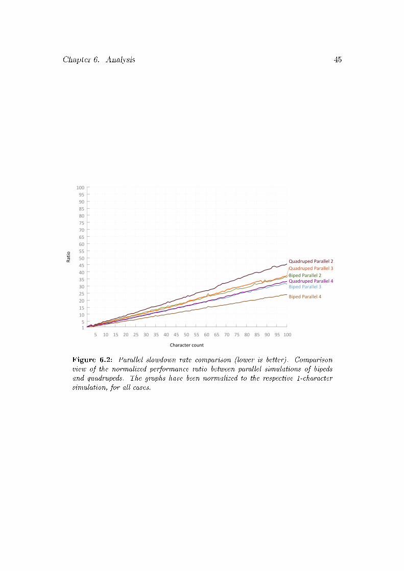
Chapter 6. Analysis 45
1 5
10
15
20
25
30
35
40
45
50
55
60
65
70
75
80
85
90
95
100
5 10 15 20 25 30 35 40 45 50 55 60 65 70 75 80 85 90 95 100
Rat
io
Character count
Quadruped Parallel 2
Quadruped Parallel 3
Biped Parallel 2Quadruped Parallel 4Biped Parallel 3
Biped Parallel 4
Figure 6.2: Parallel slowdown rate comparison (lower is better). Comparisonview of the normalized performance ratio between parallel simulations of bipedsand quadrupeds. The graphs have been normalized to the respective 1-charactersimulation, for all cases.

Chapter 6. Analysis 46
0
0.05
0.1
0.15
0.2
0.25
0.3
799 0 100 200 300 400 500 600 700
Milliseconds
Step
(a) Simulation of 35 biped charactersfor 4 parallel invocations. Executiontime peak visible between frame 700and 799.
0
0.05
0.1
0.15
0.2
0.25
0.3
799 0 100 200 300 400 500 600 700
Milliseconds
Step
(b) Second simulation of 35 bipedcharacters for 4 parallel invocations.No peak between frame 700 and 799occurred.
Figure 6.3: Random outliers in the per-frame measurement. Both graphs rep-resent the simulation of 35 biped characters over 4 threads. In graph (a) a largepeak is visible near the end of the simulation. The second graph (b) represents are-run of the same settings.
within the group of parallel measurements for bipeds and quadrupeds respectively.Performance di�erence based on leg count is statistically signi�cant for the
serial result over the whole range, without any standard deviation overlap. Thisis true when comparing the parallel measurements between leg counts as well, butonly for more than 5 characters and with the exception of three peaks registeredwithin the inclusive range of 17 to 35 characters. These peaks were caused byrandom outliers in the per-frame measurement, where one frame exhibited a peakin the execution time. Re-runs of the experiment shows that the peaks appearat random, as seen in Figure 6.3. All average measurements and their standarddeviations have been combined in Figure 6.4.
The trend of the results show an almost linear increase, with only a veryslight overall upwards curvature, most discernible in the serial simulation for thequadruped. A comparison of the quadruped simulation results and a linear trendgraph, �tted using linear regression is shown in Figure 6.5.
6.4 Summary
This chapter provided an analysis of the measurement data provided from theresults. It presented additional graphs of the slowdown rate of all measurements.In Chapter 7 the thesis is concluded with discussion of the results and possibilitiesfor future work. It summarises the work and contribution as well as providescomparisons to related work.

Chapter 6. Analysis 47
0 0.05
0.1 0.15
0.2 0.25
0.3 0.35
0.4 0.45
0.5 0.55
0.6 0.65
0.7 0.75
0.8 0.85
0.9 0.95
1 1.05
1.1 1.15
1.2
1 5 10 15 20 25 30 35 40 45 50 55 60 65 70 75 80 85 90 95 100
Mill
isec
on
ds
Quadruped Characters
Quadruped Serial
Quadruped Parallel 2
Quadruped Parallel 3
Quadruped Parallel 4
Biped Serial
Biped Parallel 2Biped Parallel 3Biped Parallel 4
Figure 6.4: Combination of Figure 5.3 and Figure 5.4.
0
0.5
1
1 100
Mill
isec
on
ds
Character Count
Linear Trend y = -0.01388 + 0.00997x
(r2 = 0.99877)
Quadruped SerialLinear Trend
(a) Trend estimation on Quadrupedserial simulations.
0
0.5
1
1.5
2
2.5
3
3.5
4
1 100 200
Mill
isec
on
ds
Character Count
Quadruped SerialLinear Trend
(b) Overview of a larger range, 1-250 characters. Trend estimation onQuadruped serial simulations.
Figure 6.5: Linear trend for the results on the serial Quadruped simulations.The estimation and the coe�cient of determination was calculated using linearregression on the execution time data by the use of the GnuPlot stats-function.The left plot (a) presents the measurement and the linear trend, while the rightplot (b) presents the same graphs with a view of a larger range.

Chapter 7
Conclusions and Future Work
In this thesis the concept of procedural animation of locomotion was presentedand an experiment was set up to measure the performance relations for such ananimation model, single- and multi-threaded. This chapter presents a summaryfollowed by conclusions that can be drawn from the results presented in Chap-ter 5 and the analysis in Chapter 6. Concluding this chapter and this thesis aresummaries of the contribution this work provides as well as the experience gainedfrom it, and how it may be utilized and advanced in the future.
7.1 Thesis Summary
The thesis presents an implementation of an algorithm for procedural animationof locomotion and outlines an experiment to measure the performance relationsbetween animation of bipedal- and quadrupedal characters, using the proceduralalgorithm.
The thesis begins by presenting the concept of procedural animation, andmore speci�cally, how it can be used to produce animation of terrestrial locomo-tion. Various methods to accomplish this were presented, both kinematic- anddynamics-driven variants. A more in-depth background was then presented ofthe dynamics-driven (physics driven) method to be implemented for performancemeasurement.
The speci�cs of the algorithm implementation were then presented in Chap-ter 3. The algorithm allows for animating both bipeds and quadrupeds. Throughthe use of virtual forces the algorithm approximates a nulli�cation of gravity bycalculating countering per-joint torques. Virtual forces also produces per-jointtorques needed in the model to allow for forwards motion of the character. PDcontrollers are further used to control internal shape of the legs (knee placement)and spine strength (in the quadruped character). The algorithm was implementedfor both serial- and parallel (on CPU) execution.
Using a greedy o�-line optimization phase, the input parameters to the al-gorithm are tweaked based on the desired gait and the character anatomy. The�nished optimized parameters then allow for real-time execution of the animationalgorithm.
48

Chapter 7. Conclusions and Future Work 49
The experiment set up to evaluate performance relations focused only on theexecution time for the algorithm itself. It executed 800 steps of simulation (about7 footsteps) for 1 to 100 characters. Both bipeds and quadrupeds were evaluatedon both serial- and parallel simulations. The experiment was automated using aseparate application which was custom made for the purpose.
7.2 Method and Implementation Discussion
The animation algorithm itself proved to have a relatively low performance im-pact compared to the application as a whole. The relationship in performancebetween bipeds, quadrupeds and between serial- and parallel execution are per-haps not that surprising. What might be surprising however is the somewhat lowperformance impact, peaking at about 1 ms for 100 quadrupeds. Given this re-sult, it might be more interesting to evaluate the overall impact of the locomotionalgorithm as well as the resulting solving done by the physics engine.
Automating the experiments proved useful due to the sheer amount of result-ing simulation time needed when running several simulations to get mean- andstandard deviation values.
The locomotion algorithm chosen proved di�cult to get working adequately.Generating plausible and working gaits using it is somewhat cumbersome. Thecharacter anatomy and the constant PD gains have to be carefully planned out.Even though many parameters are automatically optimized, the current local op-timization does require starting parameters which are somewhat plausible. Otheroptimization algorithms were not tested in this thesis, but other algorithms, suchas covariance matrix adaptation have been applied successfully in previous worksas well to optimize parameters for locomotion [14].
The gait can be optimized without motion capture data, in this thesis theresult of the IK solvers were used as a simpli�ed substitute (to reward bendingof the legs), for instance. However, the resulting quality has not been analysed.
One should expect the optimization and design of gaits to be quite time con-suming. Finding robust gaits is especially time consuming. Given correct startingconditions, optimization took about 15-30 minutes (100-300 generations) for thecharacters in this thesis. For better results, about 3-4 optimizations were ranwith incrementing lengths, on its preceding results. However, the characters inthis thesis were not optimized for turbulence and thus easily trips and falls overwhen interacted with. More thorough optimizations have been recorded to takeabout 2-12 hours [9, 13, 14].
When choosing similar methods for implementation in for example games, oneshould carefully consider if the extra amount of time needed is worth it for the ex-tra realism that a physics-driven propulsive locomotion method gives. Especiallythe extra amount of work needed by those tweaking the gait and making it robust.A simple character redesign could results in hours of optimizing work, which in

Chapter 7. Conclusions and Future Work 50
the worst case might not even �nd a pleasing gait. A kinematically-driven methodmight be su�cient in many cases.
The method tests 1-100 characters. The results show an almost linear slow-down in this range with just a slight inclination upwards.
The number of animated characters in an actual game will vary depending onthe game. The game Madden NFL 10 by Electronic Arts for instance, reportedthe need to animate about 100 characters on the �eld in real-time [18]. The tech-nical solution used to animate a character in a game might vary as well dependingon on its current level-of-detail (LOD) setting [33]. LOD in turn may for instancedepend on rendering distance or run-time performance. Which means that for aphysically simulated locomotion solution, a situation were 100 characters or moreare displayed, a LOD system could determine that only some need to be physi-cally simulated, while others use less intensive methods. The results presented inthis thesis shows that it is possible, performance-wise, to simulate locomotion fora similar amount of characters with a pose-driven feedback method, in real-time.
7.3 Conclusions
The research question posed in Chapter 1 queried what real-time performancerelations could be observed between a single-threaded and multi-threaded execu-tion of a pose-driven feedback locomotion algorithm, for groups of characters andfor varying amounts of legs.
Given the experiment results, we can discern that slowdown will scale almostlinearly for 1-100 characters. The quadrupedal slowdown rate (when increasingcharacter count) is somewhat higher than the slowdown rate of the biped. Thesimulation of the quadruped is also overall more performance intensive, takingroughly 3 times longer to compute. This might be due to the extra force calcu-lations needed for the spine (4 spine links for this experiment).
Multi-threading of the algorithm as done in this thesis provided almost ahalving of the execution time when going from serial execution to 2 parallelinvocations, in the case of 100 characters (both quadrupeds and bipeds), withdiminishing returns for further increasing of the parallel invocations. Althoughthe parallelization do allow for performance improvements of the algorithm; giventhe context presented in this thesis, a parallelization on the scope done here isquestionable in its e�ciency. Larger bottlenecks are already apparent, and work-load distribution could probably be done in another manner for better overalle�ciency.

Chapter 7. Conclusions and Future Work 51
7.4 Contribution and Comparisons
This thesis presented a �rst thorough look into the performance aspects of atypical pose-driven feedback procedural animation algorithm for physics-drivenlocomotion. Compared to previous works, relation in execution time betweenleggedness and character counts are presented, as well as an analysis of the exe-cution time slowdown rates.
These measurement provide a basis of comparison for further performanceevaluations of similar algorithms. The results presented can also be used todecide the relevance and usefulness of implementing this algorithm.
A novel implementation was made which generalized existing biped- andquadruped locomotion simulation solutions to allow for both, using the samesimulator. The source code for the implementation has been made available asopen source1 for further studies or derivative works.
7.5 Future Work
As the performance impact of the algorithm for the evaluated population countof characters is relatively low, it would be of interest to evaluate the overallimpact of the locomotion algorithm combined with the physics solver. For suchan experiment it would be of interest to compare the impact and di�erences forseveral available physics solvers.
Given a context other than real-time interactive applications, or given envi-ronments with smaller physics bottlenecks, it might also be motivated to measuremuch larger simulated character population counts as well.
This thesis evaluated simple bipeds and quadrupeds, but it might be interest-ing to broaden this scope to include insects, spiders or fantasy characters with anyleg count. Alien anatomies might even call for branching limbs, something thatno doubt could open up new interesting challenges to �nd physically simulatedgaits for.
It could also be interesting to evaluate what results a combined locomotion-and physics solver might give. To �nd out what optimizations could be made ina specialized context like that and if it provided di�ering results. Such a solutionmight be adaptable for GPGPU execution and evaluation as well, as a combinedlocomotion- and physics compute-solution might lessen the amount of read- andwrite operations to the GPU which might have been a bottleneck for a GPGPUdynamics-driven algorithm with a standalone physics solver.
This thesis covered only one type of physics-driven locomotion algorithm.There exist others for which performance data is also lacking, such as the alter-natives presented in Chapter 2. One could perform a more extensive quality- and
1www.github.com/jarllarsson/promenade (Made available 2015-02-08)

Chapter 7. Conclusions and Future Work 52
performance evaluation, over several di�erent algorithms, along with a measure-ment in implementation and optimization complexity.
Finally, what would be really interesting, is to actually successfully implementa dynamics-driven propulsive locomotion system in a game or other interactiveapplication. A game with a similar premise like Spore for example, in which theuser can design weird and wonderful fantasy creatures, and then see them cometo life. To simulate such creatures using physics, without too much failure andwithin the strict time scopes of a game is a complex but alluring task.

References
[1] R. M. N. Alexander, Principles of Animal Locomotion. Princeton UniversityPress, 2003.
[2] G. M. Amdahl, �Validity of the Single Processor Approach to AchievingLarge Scale Computing Capabilities,� in Proc AFIPS Conf, vol. 30. AFIPSPress, 1967, pp. 483�485.
[3] D. H. Bailey, �Twelve Ways to Fool the Masses When Giving PerformanceResults on Parallel Computers,� 1991.
[4] F. G. Barth, A spider's world: senses and behavior. Springer Science andBusiness Media, 2002.
[5] J. Bates, �The role of emotion in believable agents,� Communications of theACM, vol. 37, no. 7, pp. 122�125, 1994.
[6] C. M. Biancardi and A. E. Minetti, �Biomechanical determinants oftransverse and rotary gallop in cursorial mammals.� The Journal ofexperimental biology, vol. 215, no. Pt 23, pp. 4144�4156, Dec. 2012.
[7] A. Boeing and T. Bräunl, �Evaluation of Real-time Physics SimulationSystems,� in Proceedings of the 5th International Conference on ComputerGraphics and Interactive Techniques in Australia and Southeast Asia, vol. 1,no. 212. Perth, Australia: ACM, 2007, pp. 281�288.
[8] S. Coros, P. Beaudoin, and M. van de Panne, �Generalized Biped WalkingControl,� ACM Transactions on Graphics, vol. 29, no. 4, p. 1, Jul. 2010.
[9] S. Coros, A. Karpathy, B. Jones, L. Reveret, and M. van de Panne, �Loco-motion Skills for Simulated Quadrupeds,� ACM Transactions on Graphics(TOG), vol. 30, no. 4, p. 59, 2011.
[10] A. Darte and G.-R. Perrin, The Data Parallel Programming Model. SpringerBerlin / Heidelberg, 1996.
[11] J. Fang, C. Joang, and D. Terzopoulos, �Modeling and Animating Myriapoda: A Real-Time Kinematic / Dynamic Approach,� no. i, pp. 203�212, 2007.
53

References 54
[12] B. R. Gaster, L. Howes, and A. M. Devices, �Can GPGPU Programming BeLiberated from the Data-Parallel Bottleneck?� Computer, vol. 45, no. 8, pp.42�52, 2012.
[13] T. Geijtenbeek, Animating Virtual Characters using Physics-Based Simula-tion, 2013.
[14] T. Geijtenbeek, M. van de Panne, and a. F. van der Stappen, �Flexiblemuscle-based locomotion for bipedal creatures,� ACM Transactions onGraphics, vol. 32, no. 6, pp. 1�11, 2013.
[15] T. M. Gri�n, R. P. Main, and C. T. Farley, �Biomechanics of quadrupedalwalking: how do four-legged animals achieve inverted pendulum-likemovements?� The Journal of experimental biology, vol. 207, no. Pt 20, pp.3545�58, Sep. 2004.
[16] J. L. Gustafson, �Reevaluating Amdahl's law,� Communications of theACM, vol. 31, no. 5, pp. 532�533, May 1988.
[17] C. Gyrling, �Creating a Character in Drake's Fortune,� www.naughtydog.com/docs/Naughty-Dog-GDC08-Creating-a-Character-in-Drakes-Fortune.pdf (Accessed 2014-03-16), 2008.
[18] J. Harmon, �Football at 60 fps: The Challenges of Rendering MaddenNFL 10,� http://www.gdcvault.com/play/1012475/Football-at-60-fps-The(Accessed 2015-02-05).
[19] C. Hecker, B. Raabe, R. W. Enslow, J. DeWeese, J. Maynard, and K. vanProoijen, �Real-time Motion Retargeting to Highly Varied User-CreatedMorphologies,� in Proceedings of ACM SIGGRAPH '08, 2008.
[20] E. S. L. Ho, H. P. H. Shum, Y.-M. Cheung, and P. C. Yuen, �Topology AwareData-Driven Inverse Kinematics,� Computer Graphics Forum, vol. 32, no. 7,2013.
[21] R. S. Johansen, �Automated Semi-Procedural Animation for CharacterLocomotion,� Master Thesis, Aarhus Universitet, Institut for Informations-og Medievidenskab, 2009.
[22] A. A. Karim, T. Gaudin, A. Meyer, A. Buendia, and S. Bouakaz, �Procedurallocomotion of multilegged characters in dynamic environments,� ComputerAnimation and Virtual Worlds, vol. 24, no. 1, pp. 3�15, 2013.
[23] B. Kenwright, �Generating Responsive Life-Like Biped Characters,� 2012.

References 55
[24] B. Kenwright, �Responsive Biped Character Stepping: When Push Comesto Shove,� 2012 International Conference on Cyberworlds, pp. 151�156, Sep.2012.
[25] B. Kenwright, �Controlled 3D Biped Stepping Animations Using the InvertedPendulum and Impulse Constraints,� 2013 International Conference onCyberworlds, pp. 326�329, Oct. 2013.
[26] B. Kenwright, �Real-Time Dynamic Multi-Character Agents,� 2013.
[27] B. Kenwright, �Real-Time Reactive Biped Characters Staying Upright andBalanced,� Transactions on Computational Science XVIII, pp. 155�171,2013.
[28] B. Kenwright, R. Davison, and G. Morgan, �Dynamic Balancing andWalkingfor Real-time 3D Characters,� 2011.
[29] J.-Y. Kim, I.-W. Park, and J.-H. Oh, �Walking Control Algorithm of BipedHumanoid Robot on Uneven and Inclined Floor,� Journal of Intelligent andRobotic Systems, vol. 48, no. 4, pp. 457�484, Jan. 2007.
[30] J.-P. Kivistö, �Real-Time Muscle Animation,� Thesis, Kajaanin ammattiko-rkeakoulu, 2012.
[31] V. Kodaganallur and A. K. Sen, �Greedy by Chance - Stochastic GreedyAlgorithms,� 2010 Sixth International Conference on Autonomic andAutonomous Systems, pp. 182�187, Mar. 2010.
[32] J. Lee, M. Samadi, Y. Park, and S. Mahlke, �Transparent CPU-GPU collaboration for data-parallel kernels on heterogeneous systems,�Proceedings of the 22nd International Conference on Parallel Architecturesand Compilation Techniques, pp. 245�255, Sep. 2013.
[33] G. Lindahl and M. A. Johansson, �LOD Techniques for Boost-ing Rendering Performance,� http://www.gdcvault.com/play/1017872/LOD-Techniques-for-Boosting-Rendering (Accessed 2015-02-05), 2013.
[34] W. D. Lister and A. Day, �Stream-based animation of real-time crowdscenes,� Computers and Graphics, vol. 36, no. 6, pp. 651�657, Oct. 2012.
[35] C. Liu, �An Analysis of the Current and Future State of 3D Facial AnimationTechniques and Systems,� Master thesis, Simon Fraser University, 2009.
[36] L. Liu, �Terrain Runner : Control , Parameterization , Composition , andPlanning for Highly Dynamic Motions,� ACM Transactions on Graphics(TOG), vol. 31, 2012.

References 56
[37] T. Macintosh, �Animation and Player Control in Uncharted 1and 2,� www.gdcvault.com/play/1012300/Animation-and-Player-Control-in(Accessed 2014-02-13), 2010.
[38] I. S. MacKenzie and C. Ware, �Lag As a Determinant of HumanPerformance in Interactive Systems,� in Proceedings of the INTERACT '93and CHI '93 Conference on Human Factors in Computing Systems, ser. CHI'93. New York, NY, USA: ACM, 1993, pp. 488�493.
[39] T. Mclaughlin, L. Cutler, and D. Coleman, �Character Rigging , Deforma-tions , and Simulations in Film and Game Production,� in ACM SIGGRAPH2011 Courses, Vancouver, British Columbia, Canada, 2011.
[40] R. P. Paul, Robot Manipulators: Mathematics, Programming, and Control: the Computer Control of Robot Manipulators, ser. Arti�cial IntelligenceSeries. MIT Press, 1981.
[41] K. Perlin, �Creating emotive responsive characters within virtual worlds,�Lecture Notes in Arti�cial Intelligence, vol. 1834, pp. 99�106, 2000.
[42] K. Perlin and A. Goldberg, �Improv : A System for Scripting InteractiveActors in Virtual Worlds,� Acm Siggraph, pp. 205�216, 1996.
[43] J. Pratt, �Virtual Model Control: An Intuitive Approach for BipedalLocomotion,� The International Journal of Robotics Research, vol. 20, no. 2,pp. 129�143, Feb. 2001.
[44] N. Pronost and A. F. V. D. Stappen, �Simple Data-Driven Control for Simu-lated Bipeds,� SCA '12: Proceedings of the ACM SIGGRAPH/EurographicsSymposium on Computer Animation, pp. 211�219, 2012.
[45] M. H. Raibert and J. K. Hodgins, �Animation of dynamic legged locomotion,�ACM SIGGRAPH Computer Graphics, vol. 25, no. 4, pp. 349�358, 1991.
[46] C. F. Rose III, P.-P. J. Sloan, and M. F. Cohen, �Artist-DirectedInverse-Kinematics Using Radial Basis Function Interpolation,� ComputerGraphics Forum, vol. 20, no. 3, pp. 239�250, Sep. 2001.
[47] D. Rosen, �Animation Bootcamp: An Indie Approachto Procedural Animation,� http://www.gdcvault.com/play/1020049/Animation-Bootcamp-An-Indie-Approach (Accessed 2015-01-31), 2014.
[48] A. Shapiro, �Building a character animation system,� Motion in Games, pp.98�109, 2011.

References 57
[49] A. Shoulson and N. Marshak, �ADAPT : The Agent Development and Pro-totyping Testbed,� in Proceedings of the ACM SIGGRAPH Symposium onInteractive 3D Graphics and Games, vol. 1, no. 212. Orlando, Florida:ACM, 2013, pp. 9�18.
[50] K. Sims, �Evolving Virtual Creatures,� in Proceedings of the 21st annualconference on Computer graphics and interactive techniques, no. July. ACM,1994, pp. 15�22.
[51] S. Singh, M. Kapadia, G. Reinman, and P. Faloutsos, �Footstep navigationfor dynamic crowds,� Somputer Animation and Virtual Worlds, vol. 22, no.April, pp. 151�158, 2011.
[52] C. Sunada, D. Argaez, S. Dubowsky, and C. Mavroidis, �A coordinatedJacobian transpose control for mobile multi-limbed robotic systems,�Proceedings of the 1994 IEEE International Conference on Robotics andAutomation, pp. 1910�1915, 1994.
[53] Y.-Y. Tsai, W.-C. Lin, K. B. Cheng, J. Lee, and T.-Y. Lee, �Real-timephysics-based 3D biped character animation using an inverted pendulummodel.� IEEE transactions on visualization and computer graphics, vol. 16,no. 2, pp. 325�37, 2010.
[54] M. Unuma, K. Anjyo, and R. Takeuchi, �Fourier Principles for Emotion-based Human Figure Animation Munetoshi Unuma.�
[55] H. Van Welbergen, B. J. H. Van Basten, a. Egges, Z. M. Ruttkay, and M. H.Overmars, �Real Time Animation of Virtual Humans: A Trade-o� BetweenNaturalness and Control,� Computer Graphics Forum, vol. 29, no. 8, pp.2530�2554, Dec. 2010.
[56] C. L. Vaughan, B. L. Davis, and J. C. O'Connor, Dynamics of Human Gait.Kiboho Publishers, 1999.
[57] J. M. Wang, S. R. Hamner, S. L. Delp, and V. Koltun, �OptimizingLocomotion Controllers Using Biologically-based Actuators and Objectives,�ACM Transactions on Graphics (TOG), vol. 31, no. 4, pp. 25:1�-25:11,2012.
[58] C. Welman and B. S. Simon, �Inverse Kinematics and Geometric Constraintsfor Articulated Figure Manipulation,� no. September, 1993.
[59] Z. Xiao and J. J. Zhang, �Motion Data Correction and ExtrapolationUsing Physical Constraints,� Ninth International Conference on InformationVisualisation (IV'05), pp. 571�576, 2005.

References 58
[60] K. K. Yin, K. Loken, and M. van de Panne, �SIMBICON: Simple BipedLocomotion Control,� 2007.