Cryogenics 63 (2014) 94–101

Contents lists available at ScienceDirect

Cryogenics

journal homepage: www.elsevier .com/locate /cryogenics

Performance optimization of a miniature Joule–Thomson cryocoolerusing numerical model

http://dx.doi.org/10.1016/j.cryogenics.2014.07.0060011-2275/� 2014 Elsevier Ltd. All rights reserved.

⇑ Corresponding author. Tel.: +91 22 2576 7522; fax: +91 22 2572 6875.E-mail addresses: pm_ardhapurkar@yahoo.com (P.M. Ardhapurkar),

matrey@iitb.ac.in (M.D. Atrey).

P.M. Ardhapurkar a,b, M.D. Atrey a,⇑a Mechanical Engineering Department, IIT Bombay, Mumbai 400 076, Indiab S.S.G.M. College of Engineering, Shegaon 444 203, India

a r t i c l e i n f o a b s t r a c t

Article history:Received 14 April 2014Received in revised form 9 July 2014Accepted 15 July 2014Available online 27 July 2014

Keywords:Joule–Thomson cryocoolerHeat exchangerOptimizationCooling capacityPerformance

The performance of a miniature Joule–Thomson cryocooler depends on the effectiveness of the heatexchanger. The heat exchanger used in such cryocooler is Hampson-type recuperative heat exchanger.The design of the efficient heat exchanger is crucial for the optimum performance of the cryocooler.

In the present work, the heat exchanger is numerically simulated for the steady state conditions andthe results are validated against the experimental data available from the literature. The area correctionfactor is identified for the calculation of effective heat transfer area which takes into account the effect ofhelical geometry. In order to get an optimum performance of the cryocoolers, operating parameters likemass flow rate, pressure and design parameters like heat exchanger length, helical diameter of coil, findimensions, fin density have to be identified. The present work systematically addresses this aspect ofdesign for miniature J–T cryocooler.

� 2014 Elsevier Ltd. All rights reserved.

1. Introduction design of Hampson-type heat exchanger is crucial due to its com-

Joule–Thomson (J–T) cryocoolers have been widely used formany applications such as cooling of infrared detectors, cryosurgeryprobes, thermal cameras, and missile guidance systems, due to theirspecial features such as simple configuration, compact structure andrapid cooldown characteristics. It consists of a recuperative heatexchanger, an expansion device, and an evaporator. Fig. 1 showsthe schematic of a J–T cryocooler. The thermodynamic performanceof these cryocoolers is mainly governed by the effectiveness of theheat exchanger. Usually, the heat exchanger is Hampson-typefinned tube heat exchanger. The finned tubes are helically woundon mandrel and shield is provided on the outside of the coil. Theworking fluid such as nitrogen, argon at high pressure flows insidethe helically coiled finned tube, and returns over the fins afterexpansion through an orifice at the end of heat exchanger. Thelow-pressure stream circulates over the finned tube surface in oppo-site direction to the high-pressure stream. The process 1–2 repre-sents the heat rejection by the hot fluid at high pressure, whereasthe process 4–5 is the heat gain by the cold fluid at low pressure.

Several researchers have worked to compute steady state perfor-mance of the J–T cryocooler [1–4]. Few studies on transient analysisof J–T cryocooler have also been reported in the literature [5–7]. The

plex geometry, variation in thermo-physical properties of fluidand thermal losses. Ng et al. [1] and Xue et al. [2] reported experi-mental and numerical study of the J–T cryocooler for steady-statecharacteristics with argon as a working fluid. Chua et al. [4] haveargued that, Ng et al. [1] and Xue et al. [2], in their numerical work,have not used the actual heat transfer area for the low pressurereturn stream in the helical heat exchanger, but have used some cor-rection factors to compute effective area of heat transfer in thereturn line. Additionally, there is very little information availablein the literature related to the effect of various operating and designparameters on the performance of the J–T cryocooler.

The design of recuperative heat exchanger for its optimum per-formance depends on many parameters such as type of fluid, massflow rate, supply pressure, and various design parameters such asheat exchanger length, fin tube diameter, helical diameter of coil,fin dimensions, and fin density. In the present work, numericalsimulation of the heat exchanger is performed to carry out theparametric study for the optimum performance of the cryocooler.

2. Numerical model of heat exchanger

2.1. Heat exchanger geometry

2.1.1. Calculation of flow area for low pressure stream in shell sideIn the present study, the specifications of the heat exchanger

are taken from the literature [1], which are given in Table 1. The

Nomenclature

A area, m2

As surface area, m2

Cp specific heat capacity, J/kg Kd diameter, mdf fin tube diameter, mDh hydraulic diameter, mDhel mean diameter of helical coil, mf friction factorG mass flux, kg/m2 sh heat transfer coefficient, w/m2 Kk thermal conductivity, w/m KL length of heat exchanger, m_m mass flow rate, kg/s

n fin density, number of fins per meterNfins/coil number of fins per coil turnP pressure, Pap perimeter of heat transfer, mPr Prandtl numberRe Reynolds numbert mean fin thickness, mT temperature, Ku mean velocity, m/s

Greek symbolDP pressure drop, Paq density, kg/m3

Subscriptsa ambientc cold fluidci capillary insideco capillary outsideh hot fluidi insidein inletm mandrelmi mandrel insidemo mandrel outsideo outsideout outletr radiations shieldsi shield insideso shield outsidew wall

P.M. Ardhapurkar, M.D. Atrey / Cryogenics 63 (2014) 94–101 95

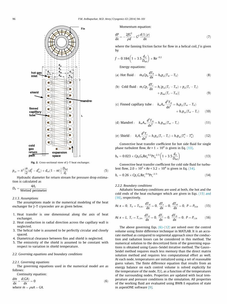
accurate calculation of the flow area for the low-pressure stream isessential for modeling the finned tube heat exchanger. Fig. 2 showsthe cross-section of the finned tube heat exchanger. In order to cal-culate flow area for low pressure stream, Ac, cross-sectional area oftube without fins and area of fins in one coil turn is subtractedfrom the total annular area between shield and mandrel. It isexpressed in Eq. (1)

Ac ¼p4ðd2

si � d2moÞ �

p4½ðDhel þ dcoÞ2 � ðDhel � dcoÞ2�

� tðdf � dcoÞ � Nfins per coil ð1Þ

where dsi is inside diameter of shield, dmo is outside diameter ofmandrel, Dhel is diameter of the helical coil, df is finned tube diam-eter, dco is the fin root diameter, and t is mean thickness of the fin.Nfins per coil represents the number of fins per turn of the coil, whichis given in Eq. (2).

Nfins per coil ¼pDhel

fin pitchð2Þ

Heatexchanger

Fig. 1. J–T cryocooler.

Alternatively, the projected area method [8] can be used to cal-culate flow area and outside perimeter of the finned tube. Accord-ing to this method, the total available free flow area on shell side,Ac, neglecting diametrical clearance is given in Eq. (3).

Ac ¼ pDhel½ðdf � dcoÞð1� n� tÞ� ð3Þ

where n is number of fins per m.

2.1.2. Calculations of surface area & Perimeter of finned tubeIn order to calculate outside perimeter of the finned tube, calcu-

lations are done for one turn of the coil neglecting the surface areaof tips of the fins. The outside surface area of finned tube is calcu-lated by subtracting surface area occupied by base of all fins ontube in one coil turn from the surface area of bare capillary tubeand the surface area of two sides of all fins in one coil turn. There-fore, surface area offered by the outer finned surface in one coilturn, As, is calculated as given in Eq. (4).

As ¼ p2 n2ðd2

f � d2coÞ þ dcoð1� ntÞ

h iDhel ð4Þ

Hence, perimeter of outer finned surface (surface area per unitaxial length), pco, is obtained as

Table 1Specifications of the heat exchanger [1].

Parameters Dimension

Inside diameter tube, dci (mm) 0.3Outside diameter tube, dco (mm) 0.5Inside diameter of mandrel, dmi (mm) 2.3Outside diameter of mandrel, dmo (mm) 2.5Inside diameter of shield, dsi (mm) 4.5Outside diameter of shield, dso (mm) 4.8Length of heat exchanger, L (mm) 50Straight length of tube (mm) 549.5Diameter of helical coil, Dhel (mm) 3.5Pitch of tube (mm) 1.0Number of turn of tube 50Height of fin (mm) 0.25Pitch of fin (mm) 0.3Thickness of fin, t (mm) 0.1Fin density (fins/mm) 3.3

Fin

Fig. 2. Cross-sectional view of J–T heat exchanger.

96 P.M. Ardhapurkar, M.D. Atrey / Cryogenics 63 (2014) 94–101

pco ¼ p2 n2ðd2

f � d2coÞ þ dcoð1� ntÞ

h iDhel

dfð5Þ

Hydraulic diameter for return stream for pressure drop estima-tion is calculated as

Dh ¼4Ac

Wetted perimeter

2.1.3. AssumptionsThe assumptions made in the numerical modeling of the heat

exchanger for J–T cryocooler are as given below.

1. Heat transfer is one dimensional along the axis of heatexchanger.

2. Heat conduction in radial direction across the capillary wall isneglected.

3. The helical tube is assumed to be perfectly circular and closelyspaced.

4. Diametrical clearance between fins and shield is neglected.5. The emissivity of the shield is assumed to be constant with

respect to variation in shield temperature.

2.2. Governing equations and boundary conditions

2.2.1. Governing equationsThe governing equations used in the numerical model are as

follows:Continuity equation:

d _mdx¼ dðGAÞ

dx¼ 0 ð6Þ

where _m ¼ quA ¼ GA.

Momentum equation:

dPdx¼ �2fG2

qd� G2 dð1=qÞ

dxð7Þ

where the fanning friction factor for flow in a helical coil, f is givenby

f ¼ 0:184 1þ 3:5dci

Dhel

� �� Re�0:2

Energy equations:

ðaÞ Hot fluid : _mhCphdTh

dx¼ hhpciðTw � ThÞ ð8Þ

ðbÞ Cold fluid : m:

cCpcdTc

dx¼ hc½pcoðTc � TwÞ þ psiðTc � TsÞ

þ pmoðTc � TmÞ� ð9Þ

ðcÞ Finned capillary tube : kwAwd2Tw

dx2 ¼ hhpciðTw � ThÞ

þ hcpcoðTw � TcÞ ð10Þ

ðdÞ Mandrel : kmAmd2Tm

dx2 ¼ hcpmoðTm � TcÞ ð11Þ

ðeÞ Shield : ksAsd2Ts

dx2 ¼ hcpsiðTs � TcÞ þ hrpsoðT4s � T4

aÞ ð12Þ

Convective heat transfer coefficient for hot side fluid for singlephase turbulent flow, Re > 1 � 104 is given in Eq. (13).

hh ¼ 0:023� CphGhRe�0:2h Pr�2=3

h 1þ 3:5dci

Dhel

� �ð13Þ

Convective heat transfer coefficient for cold side fluid for turbu-lent flow, 2.0 � 103 < Re < 3.2 � 104 is given in Eq. (14).

hc ¼ 0:26� CpcGcRe�0:4c Pr�2=3

c ð14Þ

2.2.2. Boundary conditionsAdiabatic boundary conditions are used at both, the hot and the

cold ends of the heat exchanger which are given in Eqs. (15) and(16), respectively.

At x ¼ 0; Th ¼ Th;in;dTw

dx¼ 0;

dTs

dx¼ 0;

dTm

dx¼ 0; P ¼ Ph;in ð15Þ

At x ¼ L; Tc ¼ Tc;in;dTw

dx¼ 0;

dTs

dx¼ 0;

dTm

dx¼ 0; P ¼ Pc;in ð16Þ

The above governing Eqs. (6)–(12) are solved over the controlvolume using finite difference technique in MATLAB. It is an accu-rate method as compared to segmental approach since the conduc-tion and radiation losses can be considered in this method. Thenumerical solution to the descretized form of the governing equa-tions is obtained using Gauss–Seidel iterative method. The Gauss–Seidel method requires much less memory than the direct matrixsolution method and requires less computational effort as well.At each node, temperatures are initialized using a set of reasonableguess values. The finite difference equation that results from anenergy balance on each control volume is solved explicitly forthe temperature of the node, T(i), as a function of the temperaturesof the surrounding nodes. Properties are updated with local tem-perature and pressure conditions in the simulation. All propertiesof the working fluid are evaluated using BWR-S equation of statein aspenONE software [9].

P.M. Ardhapurkar, M.D. Atrey / Cryogenics 63 (2014) 94–101 97

3. Validation of the model

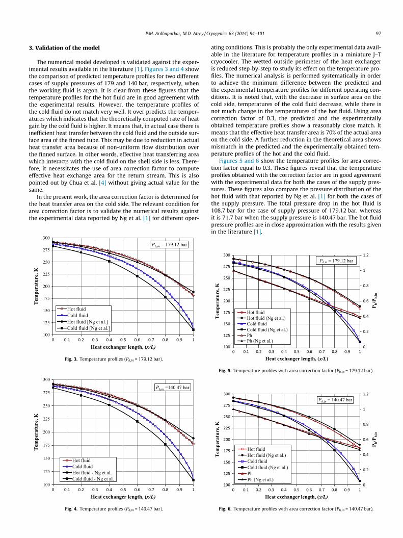
The numerical model developed is validated against the exper-imental results available in the literature [1]. Figures 3 and 4 showthe comparison of predicted temperature profiles for two differentcases of supply pressures of 179 and 140 bar, respectively, whenthe working fluid is argon. It is clear from these figures that thetemperature profiles for the hot fluid are in good agreement withthe experimental results. However, the temperature profiles ofthe cold fluid do not match very well. It over predicts the temper-atures which indicates that the theoretically computed rate of heatgain by the cold fluid is higher. It means that, in actual case there isinefficient heat transfer between the cold fluid and the outside sur-face area of the finned tube. This may be due to reduction in actualheat transfer area because of non-uniform flow distribution overthe finned surface. In other words, effective heat transferring areawhich interacts with the cold fluid on the shell side is less. There-fore, it necessitates the use of area correction factor to computeeffective heat exchange area for the return stream. This is alsopointed out by Chua et al. [4] without giving actual value for thesame.

In the present work, the area correction factor is determined forthe heat transfer area on the cold side. The relevant condition forarea correction factor is to validate the numerical results againstthe experimental data reported by Ng et al. [1] for different oper-

100

125

150

175

200

225

250

275

300

0 0.1 0.2 0.3 0.4 0.5 0.6 0.7 0.8 0.9 1

Tem

pera

ture

, K

Heat exchanger length, (x/L)

Ph,in = 179.12 bar

Hot fluidCold fluidHot fluid [Ng et al.]Cold fluid [Ng et al.]

Fig. 3. Temperature profiles (Ph,in = 179.12 bar).

100

125

150

175

200

225

250

275

300

0 0.1 0.2 0.3 0.4 0.5 0.6 0.7 0.8 0.9 1

Tem

pera

ture

, K

Heat exchanger length, (x/L)

Ph,in =140.47 bar

Hot fluidCold fluidHot fluid - Ng et al.Cold fluid - Ng et al.

Fig. 4. Temperature profiles (Ph,in = 140.47 bar).

ating conditions. This is probably the only experimental data avail-able in the literature for temperature profiles in a miniature J–Tcryocooler. The wetted outside perimeter of the heat exchangeris reduced step-by-step to study its effect on the temperature pro-files. The numerical analysis is performed systematically in orderto achieve the minimum difference between the predicted andthe experimental temperature profiles for different operating con-ditions. It is noted that, with the decrease in surface area on thecold side, temperatures of the cold fluid decrease, while there isnot much change in the temperatures of the hot fluid. Using areacorrection factor of 0.3, the predicted and the experimentallyobtained temperature profiles show a reasonably close match. Itmeans that the effective heat transfer area is 70% of the actual areaon the cold side. A further reduction in the theoretical area showsmismatch in the predicted and the experimentally obtained tem-perature profiles of the hot and the cold fluid.

Figures 5 and 6 show the temperature profiles for area correc-tion factor equal to 0.3. These figures reveal that the temperatureprofiles obtained with the correction factor are in good agreementwith the experimental data for both the cases of the supply pres-sures. These figures also compare the pressure distribution of thehot fluid with that reported by Ng et al. [1] for both the cases ofthe supply pressure. The total pressure drop in the hot fluid is108.7 bar for the case of supply pressure of 179.12 bar, whereasit is 71.7 bar when the supply pressure is 140.47 bar. The hot fluidpressure profiles are in close approximation with the results givenin the literature [1].

0

0.2

0.4

0.6

0.8

1

1.2

100

125

150

175

200

225

250

275

300

0 0.1 0.2 0.3 0.4 0.5 0.6 0.7 0.8 0.9 1

P h/P

h,in

Tem

pera

ture

, K

Heat exchanger length, (x/L)

Hot fluidHot fluid (Ng et al.)Cold fluidCold fluid (Ng et al.)PhPh (Ng et al.)

Ph,in = 179.12 bar

Fig. 5. Temperature profiles with area correction factor (Ph,in = 179.12 bar).

0

0.2

0.4

0.6

0.8

1

1.2

100

125

150

175

200

225

250

275

300

0 0.1 0.2 0.3 0.4 0.5 0.6 0.7 0.8 0.9 1

P h/P

h,in

Tem

pera

ture

, K

Heat exchanger length, (x/L)

Ph,in = 140.47 bar

Hot fluidHot fluid (Ng et al.)Cold fluidCold fluid (Ng et al.)PhPh (Ng et al.)

Fig. 6. Temperature profiles with area correction factor (Ph,in = 140.47 bar).

0.2

0.3

0.4

0.5

0.6

0.7

0.95

0.96

0.97

0.98

0.99

1

Pres

sure

dro

p in

col

d flu

id, b

ar

Eff

ectiv

enes

s of h

eat e

xcha

nger

Working fluid: ArgonCase 1:

Ph,in = 179.12 bar, Pc,in= 1.7272 barTh,in = 291.49 K, Tc,in = 110.36 K

Case 2:Ph,in = 140.47 bar, Pc,in = 1.3426 barTh,in = 291.94 K, Tc,in = 108.7 K

Case 1: EffectivenessCase 2: EffectivenessCase 1: Pressure drop

98 P.M. Ardhapurkar, M.D. Atrey / Cryogenics 63 (2014) 94–101

The predicted temperatures of the cold fluid at the outlet of theheat exchanger are compared with the experimental data and thesimulation results from the literature. Table 2 gives the validationof the numerical results in tabular form for the outlet temperatureof the cold fluid as well as relative errors between predicted andactual results. Table 3 compares the results for pressure drop inboth, the hot and the cold fluid against the literature data. It isnoted that the pressure drop in both, the hot and the cold fluid,are comparable with that of the literature values. It is clear fromTable 2 that the predicted temperature of the cold fluid at the out-let is close to experimental values. The relative error in the simu-lated results for the outlet temperatures of the fluid are within1% limit.

0.10.942.7 2.8 2.9 3 3.1 3.2 3.3 3.4 3.5 3.6 3.7

Fin density, fins/mm

Case 2: Pressure drop

Fig. 7. Effect of fin density on the heat exchanger performance.

4. Performance optimization of cryocooler

Performance of the J–T cryocooler depends on various designand operating parameters. The design parameters considered inthe present work are fin density, coil diameter, heat exchangerlength, while the operating parameters considered are workingfluid, mass flow rate, and supply pressure. In the following section,effect of design parameters is studied for a J–T cryocooler, specifi-cations of which are given in Table 1, while in the later section, theperformance optimization is attempted for this specific design ofthe J–T cryocooler. The optimization is carried out to maximizecooling capacity at low temperature for which J–T cryocooler isdesigned. The parameters optimized are heat exchanger length,pressure, mass flow rate for different working fluids, argon andnitrogen. The constraints in optimizing different parameters areas given below.

(a) The condition of the hot stream at the outlet of the heatexchanger should be such that the state of the working fluidafter isenthalpic expansion should fall in vapor dome so asto have sufficient cooling effect.

(b) Pressure drop in the return line should be kept minimum sothat the net pressure at the return line outlet remains aboveatmospheric pressure.

4.1. Effect of geometry on performance of the cryocooler

The effect of the design parameters of the heat exchanger suchas fin density, helical coil diameter on the performance of the cryo-cooler is studied to determine its optimum performance.

Table 2Prediction of heat exchanger temperatures.

Input conditions Tc,out (K) (N

Ph,in (bar) Pc,in (bar) Th,in (K) Tc,in (K) Experimen

179.12 1.7272 291.49 110.36 282.57169.86 1.7460 291.40 110.42 283.73160.1 1.6362 292.25 109.9 284.77149.66 1.4713 292.14 109.28 284.90140.47 1.3426 291.94 108.70 284.98

Table 3Prediction of pressure drop.

Ph,in (bar) Pc,in (bar) Pressure drop (bar) (Ng et a

Hot fluid

179.12 1.7272 109.26140.47 1.3426 77.25

4.1.1. Effect of fin density on heat exchanger performanceFin density is optimized with the objective of maximizing effec-

tiveness of the heat exchanger and with the constraints of allow-able pressure drop in the cold fluid. Fig. 7 shows the effect of findensity on the effectiveness of the heat exchanger for the case withthe supply pressure of 179.12 bar and 140.47 bar. It is observedthat with the increase in fin density, the effectiveness of the heatexchanger increases due to increased area of heat transfer. How-ever, increase in effectiveness is less beyond certain fin density,i.e. 3.3 fins per mm. This is due to more resistance to flow on thecold side. Fig. 7 also shows the effect of fin density on the pressuredrop in the cold fluid for both the cases of supply pressures. It isnoted that the pressure drop on cold side increases with increasein fin density for both the cases of supply pressures. It is also foundthat the pressure drop in the cold fluid increases with the increasein supply pressure for any value of fin density. The pressure drop inthe cold fluid is more crucial since increased pressure drop leads tomore power consumption. The allowable pressure drop in the coldfluid for the case of supply pressure of 179 bar is 0.7 bar, while it is0.35 bar for the case of supply pressure of 140 bar. Therefore, opti-mum fin density for both the operating pressures is 3.3.

4.1.2. Effect of helical diameter of heat exchanger on performance ofthe cryocooler

In order to study the effect of the helical diameter of the heatexchanger on the performance of the cryocooler, two cases of thehelical diameters, 3.5 mm and 4.5 mm are considered. The heat

g et al. [1]) Tc,out (K) numerical Relative error (%)

tal Numerical

282.85 284.38 +0.63282.90 285.53 +0.63284.07 285.23 0.161284.19 284.74 �0.056284.15 284.96 �0.007

l. [1]) Pressure drop (bar)

Cold fluid Hot fluid Cold fluid

0.67 108.69 0.5290.3176 71.7 0.385

0

20

40

60

80

100

120

140

160

180

200

80 100 120 140 160 180 200 220 240 260 280 300

Ent

halp

y di

ffer

ence

, kJ/

kg

Temperature, K

50 MPa

40 MPa

30 MPa

20 MPa

10 MPa

Argon

Fig. 9. Ideal cooling capacity for argon.

P.M. Ardhapurkar, M.D. Atrey / Cryogenics 63 (2014) 94–101 99

transfer area is kept constant for both the cases. Therefore, thelength of the heat exchanger decreases to 38.9 mm from 50 mmwith the increase in helical diameter from 3.5 mm to 4.5 mm.The cooling capacity is calculated at 110 K keeping all the param-eters constant for both the cases. Supply pressure for argon is fixedat 200 bar.

Fig. 8 gives the comparison of the cooling capacity variationwith respect to mass flow rate for two different cases of the helicaldiameter. It is observed that the cooling capacity is more for theheat exchanger having less helical diameter. This is due to higherturbulence due to secondary flows in the heat exchanger. Due toincrease in the helical diameter, the heat transfer rate decreaseswhile there is compensation in pressure drop in the cold fluiddue to reduced flow path for the cold fluid. Therefore, the decreasein the maximum cooling capacity is only 3.7% with the increase inthe helical diameter for the above case. The maximum coolingcapacity corresponds to the same mass flow rate of 0.28 g/s forboth the cases.

140

160

180

200

ce, k

J/kg

50 MPa40 MPa30 MPa20 MPa

Nitrogen

4.2. Effect of operating parameters on performance of the cryocooler

In this section, the effect of the working fluid and other operat-ing parameters such as mass flow rate, supply pressure on thecooling capacity is analyzed to determine the optimum perfor-mance of the cryocooler.

0

20

40

60

80

100

120

80 100 120 140 160 180 200 220 240 260 280 300

Ent

halp

y di

ffer

en

Temperature, K

10 MPa

Fig. 10. Ideal cooling capacity for nitrogen.

4.2.1. Effect of working fluidUsually, nitrogen and argon are used as working fluids in the J–T

cryocooler. The properties of the fluid significantly affect the per-formance of the cryocooler. In a perfect recuperator (i.e. one withan infinite conductance), maximum possible refrigeration capacityper unit mass flow is the minimum value of the specific enthalpydifference (isothermal J–T effect) over the entire operating temprange. In order to study the effect of fluid on the performance ofthe cryocooler, ideal cooling capacities are calculated for two dif-ferent fluids: nitrogen and argon. Figures 9 and 10 show variationin the specific enthalpy difference with respect to supply pressurefor argon and nitrogen, respectively. It is observed that theenthalpy difference between the two pressures decreases at highertemperatures since gas behaves more like an ideal gas. The mini-mum enthalpy difference at temperature of 300 K increases withthe increase in supply pressure up to 40 MPa. At pressures higherthan 40 MPa, the increase in ideal cooling capacity is less for argon;however, there is decrease in cooling capacity in the case of nitro-gen for increase in supply pressure beyond 40 MPa. The maximum

0

1

2

3

4

5

6

7

8

0.05 0.1 0.15 0.2 0.25 0.3 0.35 0.4 0.45

Coo

ling

capa

city

, W

Mass flow rate, g/s

Th,in = 300 KTc,in = 110 KPh,in = 200 barPc,in = 1.7 bar

Helical dia. = 3.5 mmHelical dia. = 4.5 mm

Fig. 8. Effect of helical diameter on performance of the cooler.

possible cooling capacity of the J–T cryocooler with the use ofnitrogen and argon is compared in Table 4. It is noted that the idealcooling capacity for argon is more than that for nitrogen for thesame operating range of temperatures and pressures.

Fig. 11 compares the cooling capacity of the J–T cryocoolerworking with argon and nitrogen for the same operating condi-tions. As pointed out in Table 4, it is found that the cooling capacityfor argon at 110 K is more than that for nitrogen at any operatingmass flow rate of the fluid. The difference in the cooling capacityincreases with the increase in the mass flow rate. The maximumcooling capacity obtained is 6.79 W at the mass flow rate of0.28 g/s for argon. In the case of nitrogen, the maximum coolingcapacity is 4.0 W only at the mass flow rate of 0.22 g/s. This isdue to reduced isothermal J–T effect for nitrogen as a workingfluid. Fig. 11 also proves that the pressure drop in the hot fluid ismore in the case of nitrogen as compared to that for the argon.Due to cumulative effect of increased pressure drop in the hot fluidand reduced isothermal J–T effect, cooling capacity is lower withthe nitrogen as a working fluid.

The pressure drop in the hot fluid is 46.8 bar corresponding tomaximum cooling capacity at 0.28 g/s for the case of argon. Fornitrogen, this pressure drop is 43.3 bar corresponding to maximumcooling capacity at 0.22 g/s. It is also noted from Fig. 11 that pres-sure drop in the hot fluid increases significantly with increase inthe mass flow rate. In the case of argon, the pressure drop in thehot fluid increases to 89.9 bar for mass flow rate of 0.38 g/s.

Table 4Maximum cooling capacity per unit mass flow rate at various supply pressures (Ph, in) and Pc,in = 1 bar.

Fluid Temp. range Specific enthalpy difference (kJ/kg) at supply pressure in MPa

10 20 30 40 50

N2 80–300 K 19.40 30.90 36.16 37.62 36.73Ar 90–300 K 18.0 32.10 41.10 46.30 48.99

0

10

20

30

40

50

60

70

80

90

100

0

1

2

3

4

5

6

7

8

0.05 0.1 0.15 0.2 0.25 0.3 0.35 0.4

Pres

sure

dro

p in

hot

flui

d, b

ar

Coo

ling

capa

city

, W

Mass flow rate, g/s

Th,in = 300 KTc,in = 110 KPh,in = 200 barPc,in = 1.7 bar

Cooling capacity - ArCooling capacity- N2Pressure drop - ArPressure drop - N2

Fig. 11. Effect of working fluid on performance of J–T cryocooler.

0

20

40

60

80

100

120

0

2

4

6

8

10

12

0.05 0.1 0.15 0.2 0.25 0.3 0.35 0.4

Pres

sure

dro

p in

hot

flui

d, b

ar

Coo

ling

capa

city

, W

Mass flow rate, g/s

Fluid: ArgonTh,in = 300 KTc,in = 110 KPc,in = 1.7 barL = 50 mm

150 bar160 bar170 bar180 bar200 bar220 bar240 bar150 bar160 bar170 bar180 bar200 bar220 bar240 bar

Cooling capacity Pressure drop in hot fluid

Fig. 13. Effect of supply pressure on performance of the cryocooler.

100 P.M. Ardhapurkar, M.D. Atrey / Cryogenics 63 (2014) 94–101

4.2.2. Effect of mass flow rate on performance of heat exchangerFig. 12 shows the effect of mass flow rate on the effectiveness of

the heat exchanger and pressure drop in the hot fluid. It is foundthat, pressure drop in the hot fluid increases significantly andeffectiveness of the heat exchanger decreases with the increasein mass flow rate.

4.2.3. Effect of supply pressure on performance of the cryocoolerFig. 13 shows the effect of supply pressure of argon on the per-

formance of the cryocooler for the input conditions of Th,in = 300 K,Tc,in = 110 K, and Pc,in = 1.7 bar. It is clear from the figure that cool-ing capacity increases with the increase in supply pressure. It canalso be seen that the optimum mass flow rate for producing max-imum cooling capacity increases with the increase in supply pres-sure. The optimal mass flow rate is 0.18 g/s for the supply pressureof 150 bar, while it increases to 0.28 g/s for the supply pressure of200 bar. Also, pressure drop in the hot fluid decreases withincrease in supply pressure. The pressure drop in the hot fluid is

0

10

20

30

40

50

60

70

80

0.96

0.965

0.97

0.975

0.98

0.985

0.05 0.1 0.15 0.2 0.25 0.3

Pres

sure

dro

p, b

ar

Eff

ectiv

enes

s of h

eat e

xcha

nger

Mass flow rate, g/s

Fluid: ArgonTh,in = 291.94 K, Tc,in = 108.7 K, Ph,in = 140.47 bar, Pc,in = 1.3426 bar

EffectivenessPressure drop - Hot fluid

Fig. 12. Effect of mass flow rate on performance the heat exchanger.

calculated to be 46.8 bar for the supply pressure of 200 bar, whileit is 39.8 bar for the supply pressure of 240 bar with mass flow0.3 g/s. This is due to the fact that both, the friction factor andthe density increase with the increase in the supply pressure. How-ever, increment in the density is more than increment in the fric-tion factor. Therefore, the cooling capacity is more with increasein supply pressure for any operating condition of mass flow rate.Additionally, it is observed that the increase in mass flow ratebeyond 0.35 g/s leads to increased pressure drop in the cold fluid.For the supply pressure greater than 180 bar, the pressure drop inthe cold fluid is more than the allowable limit to have positivepressure at the suction to the compressor. Therefore, maximumlimit on the operating mass flow rate is 0.35 g/s for the supplypressures greater than 180 bar. However, for the lower supplypressures, limit on the maximum mass flow rate is determineddue to cooling capacity.

On the basis of above study, the optimum size of the heatexchanger to have maximum cooling capacity at low temperatureof 110 K is determined for the given operating conditions. For this,high pressure and low pressure are 200 bar and 1.7 bar, respec-tively. It is clear from Fig. 13 that, for the heat exchanger lengthof 50 mm, a maximum cooling capacity of 6.8 W at 110 K can beachieved with supply pressure of 200 bar and mass flow rate of0.28 g/s. Also, for lower mass flow rate of 0.2 g/s, the cooling capac-ity obtained is 5.84 W; however, this is not the maximum coolingcapacity that can be obtained from the specified heat exchanger.Therefore, an optimum size of the heat exchanger should be foundout for the specific mass flow rate.

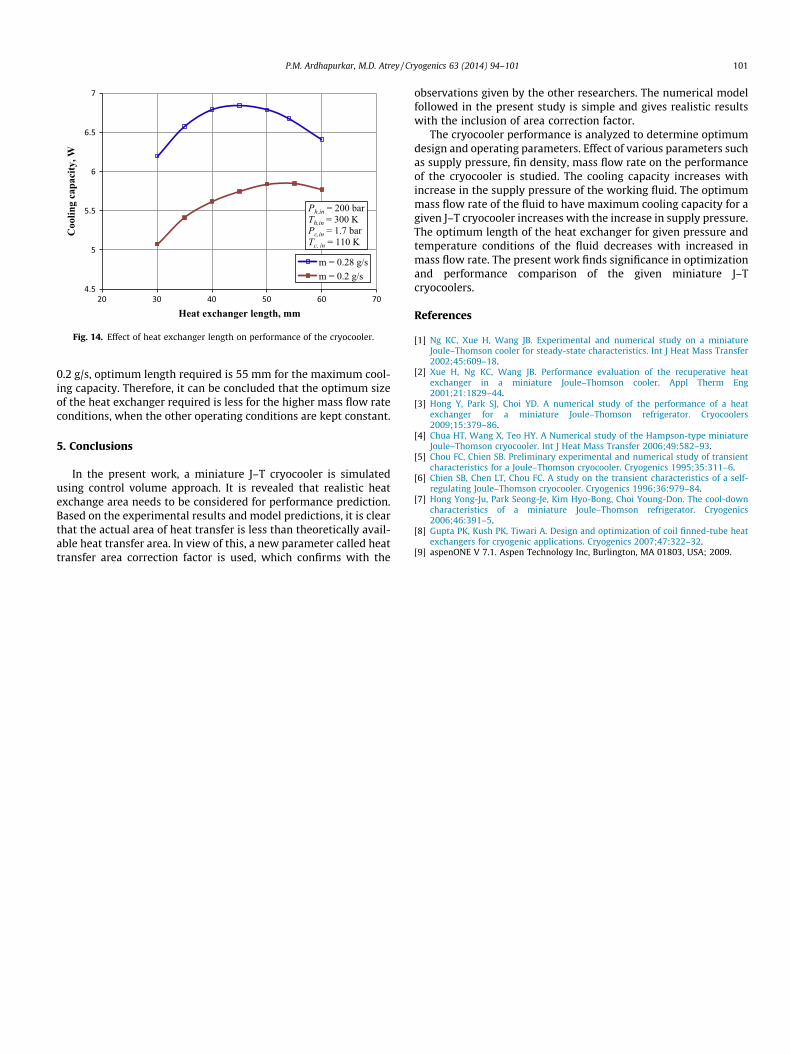
Fig. 14 shows the variation in cooling capacity with respect tothe heat exchanger length. Cooling capacity decreases with theincrease in length beyond optimum value because of increase inpressure drop in the heat exchanger. It is found from Fig. 14 thatthe optimum heat exchanger length required is 45 mm only, tohave maximum cooling capacity of 6.84 W when the mass flowrate is 0.28 g/s. On the other hand, when the mass flow rate is

4.5

5

5.5

6

6.5

7

20 30 40 50 60 70

Coo

ling

capa

city

, W

Heat exchanger length, mm

Ph,in = 200 barTh,in = 300 KPc,in = 1.7 barTc, in = 110 K

m = 0.28 g/sm = 0.2 g/s

Fig. 14. Effect of heat exchanger length on performance of the cryocooler.

P.M. Ardhapurkar, M.D. Atrey / Cryogenics 63 (2014) 94–101 101

0.2 g/s, optimum length required is 55 mm for the maximum cool-ing capacity. Therefore, it can be concluded that the optimum sizeof the heat exchanger required is less for the higher mass flow rateconditions, when the other operating conditions are kept constant.

5. Conclusions

In the present work, a miniature J–T cryocooler is simulatedusing control volume approach. It is revealed that realistic heatexchange area needs to be considered for performance prediction.Based on the experimental results and model predictions, it is clearthat the actual area of heat transfer is less than theoretically avail-able heat transfer area. In view of this, a new parameter called heattransfer area correction factor is used, which confirms with the

observations given by the other researchers. The numerical modelfollowed in the present study is simple and gives realistic resultswith the inclusion of area correction factor.

The cryocooler performance is analyzed to determine optimumdesign and operating parameters. Effect of various parameters suchas supply pressure, fin density, mass flow rate on the performanceof the cryocooler is studied. The cooling capacity increases withincrease in the supply pressure of the working fluid. The optimummass flow rate of the fluid to have maximum cooling capacity for agiven J–T cryocooler increases with the increase in supply pressure.The optimum length of the heat exchanger for given pressure andtemperature conditions of the fluid decreases with increased inmass flow rate. The present work finds significance in optimizationand performance comparison of the given miniature J–Tcryocoolers.

References

[1] Ng KC, Xue H, Wang JB. Experimental and numerical study on a miniatureJoule–Thomson cooler for steady-state characteristics. Int J Heat Mass Transfer2002;45:609–18.

[2] Xue H, Ng KC, Wang JB. Performance evaluation of the recuperative heatexchanger in a miniature Joule–Thomson cooler. Appl Therm Eng2001;21:1829–44.

[3] Hong Y, Park SJ, Choi YD. A numerical study of the performance of a heatexchanger for a miniature Joule–Thomson refrigerator. Cryocoolers2009;15:379–86.

[4] Chua HT, Wang X, Teo HY. A Numerical study of the Hampson-type miniatureJoule–Thomson cryocooler. Int J Heat Mass Transfer 2006;49:582–93.

[5] Chou FC, Chien SB. Preliminary experimental and numerical study of transientcharacteristics for a Joule–Thomson cryocooler. Cryogenics 1995;35:311–6.

[6] Chien SB, Chen LT, Chou FC. A study on the transient characteristics of a self-regulating Joule–Thomson cryocooler. Cryogenics 1996;36:979–84.

[7] Hong Yong-Ju, Park Seong-Je, Kim Hyo-Bong, Choi Young-Don. The cool-downcharacteristics of a miniature Joule–Thomson refrigerator. Cryogenics2006;46:391–5.

[8] Gupta PK, Kush PK, Tiwari A. Design and optimization of coil finned-tube heatexchangers for cryogenic applications. Cryogenics 2007;47:322–32.

[9] aspenONE V 7.1. Aspen Technology Inc, Burlington, MA 01803, USA; 2009.