persamaan diferensial biasa - istiarto.staff.ugm.ac.id persamaan diferensial biasa.pdf · persamaan...

Ordinary Differential Equations – ODE

PERSAMAAN DIFERENSIAL BIASA

https://istiarto.staff.ugm.ac.id


Persamaan Diferensial Biasa2

❑ Acuan

❑ Chapra, S.C., Canale R.P., 1990, Numerical Methods for Engineers, 2nd

Ed., McGraw-Hill Book Co., New York.

◼ Chapter 19 dan 20, hlm. 576-640.


Persamaan Diferensial3

FU = −c v

FD = m g

❑ Benda bermassa m jatuh bebas dengan

kecepatan v

m

FF

m

Fa UD +== Hukum Newton II

c = drag coefficient (kg/s)

g = gravitational acceleration (m/s2)

persamaan diferensial

suku diferensial laju perubahan (rate of change)

vm

cg

t

v−=

d

d

t

v

d

d


Persamaan Diferensial4

FU = −c v

FD = m g

❑ Sebuah benda jatuh bebas

❑ Jika pada saat awal benda dalam keadaan diam:

syarat awal (initial condition)( ) 00 ==tv

vm

cg

t

v−=

d

d

( ) ( ) tmcec

gmtv −−= 1


Persamaan Diferensial

❑ Persamaan diferensial

❑ v variabel tak bebas (dependent variable)

❑ t variabel bebas (independent variable)

❑ Persamaan diferensial biasa

(ordinary differential equations, ODE)

❑ hanya terdiri dari satu variabel bebas

❑ Persamaan diferensial parsial

(partial differential equations, PDE)

❑ terdiri dari dua atau lebih variabel bebas

vm

cg

t

v−=

d

d

vm

cg

t

v−=

d

d

02

2

=

−

x

CD

t

C

5


Persamaan Diferensial

❑ Persamaan diferensial

❑ tingkat (order) tertinggi suku derivatif

❑ Persamaan diferensial tingkat-1

❑ suku derivatif bertingkat-1

❑ Persamaan diferensial tingkat-2

❑ suku derivatif bertingkat-2

vm

cg

t

v−=

d

d

0d

d

d

d2

2

=++ kxt

xc

t

xm

6


Persamaan Diferensial Biasa

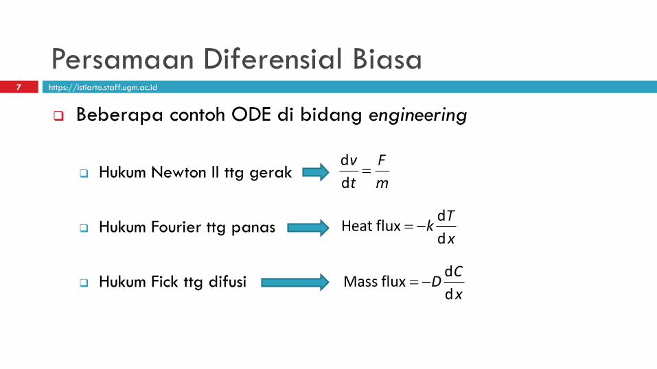
❑ Beberapa contoh ODE di bidang engineering

❑ Hukum Newton II ttg gerak

❑ Hukum Fourier ttg panas

❑ Hukum Fick ttg difusi

m

F

t

v=

d

d

x

Tk

d

dflux Heat −=

x

CD

d

dflux Mass −=

7



15.81045.0 234 ++−+−= xxxxy

5.820122d

d 23 +−+−= xxxx

y

diketahui:

fungsi polinomial tingkat 4

diperoleh: ODE

di-diferensial-kan



0

1

2

3

4

5

0 1 2 3 4

-8

-4

0

4

8

0 1 2 3 4

9

y = -0.5x

4 + 4x3 -10x

2 +8.5x+1

dy

dx= -2x

3 +12x2 -20x+8.5

XX

x

y

d

dY



5.820122d

d 23 +−+−= xxxx

y

diketahui: ODE

fungsi asal

di-integral-kan

( )

Cxxxxy

xxxxy

++−+−=

+−+−= 5.81045.0

d5.820122

234

23

C disebut konstanta integrasi



-8

-4

0

4

8

0 1 2 3 4

-4

0

4

8

0 1 2 3 4

11

Cxxxxy ++−+−= 5.81045.0 234

5.820122d

d 23 +−+−= xxxx

y

XX

x

y

d

dY

C = 3

2

1

0

−1

−2



Cxxxxy ++−+−= 5.81045.0 234

❑ Hasil dari integrasi adalah sejumlah tak berhingga polinomial.

❑ Penyelesaian yang unique (tunggal, satu-satunya) diperoleh dengan

menerapkan suatu syarat, yaitu pada titik awal x = 0, y = 1 → ini disebut

dengan istilah syarat awal (initial condition).

❑ Syarat awal tersebut menghasilkan C = 1.

15.81045.0 234 ++−+−= xxxxy



❑ Syarat awal (initial condition)

❑ mencerminkan keadaan sebenarnya, memiliki arti fisik

❑ pada persamaan diferensial tingkat n, maka dibutuhkan sejumlah n

syarat awal

❑ Syarat batas (boundary conditions)

❑ syarat yang harus dipenuhi tidak hanya di satu titik di awal saja, namun

juga di titik-titik lain atau di beberapa nilai variabel bebas yang lain



❑ Metode penyelesaian ODE

❑ Metode Euler

❑ Metode Heun

❑ Metode Euler Modifikasi (Metode Poligon)

❑ Metode Runge-Kutta


Metode Euler

Penyelesaian ODE15

http://istiarto.staff.ugm.ac.id


Metode Satu Langkah

❑ Dikenal pula sebagai metode satu

langkah (one-step method)

❑ Persamaan:

❑ new value = old value + slope x step size

❑ Dalam bahasa matematika:

❑ jadi, slope atau gradien φ dipakai untuk

meng-ekstrapolasi-kan nilai lama yi ke

nilai baru yi+1 dalam selang h

hyy ii +=+1

1616

xi xi+1

step size = h

x

y

hyy ii +=+1

slope = φ


Metode Satu Langkah

❑ Semua metode satu langkah dapat

dinyatakan dalam persamaan tsb.

❑ Perbedaan antara satu metode dengan

metode yang lain dalam metode satu

langkah ini adalah perbedaan dalam

menetapkan atau memperkirakan slope φ.

❑ Salah satu metode satu langkah adalah

Metode Euler.

hyy ii +=+1

17

xi xi+1

step size = h

x

y

slope = φ

hyy ii +=+1


Metode Euler18

❑ Dalam Metode Euler, slope di xi diperkirakan

dengan derivatif pertama di titik (xi,yi).

❑ Metode Euler dikenal pula dengan nama

Metode Euler-Cauchy.

❑ Jadi nilai y baru diperkirakan berdasarkan

slope, sama dengan derivatif pertama di titik x,

untuk mengekstrapolasikan nilai y lama secara

linear dalam selang h ke nilai y baru.

( )hyxfyy iiii ,1 +=+

( )ii yx

iix

yyxf

,d

d, ==


Metode Euler19

❑ Pakailah Metode Euler untuk mengintegralkan ODE di bawah ini, dari x = 0

s.d. x = 4 dengan selang langkah h = 0.5:

( ) 5.820122d

d, 23 +−+−== xxx

x

yyxf

❑ Syarat awal yang diterapkan pada ODE tsb adalah bahwa di titik x= 0,

y = 1

❑ Ingat, penyelesaian eksak ODE di atas adalah:

15.81045.0 234 ++−+−= xxxxy


Metode Euler20

❑ Selang ke-1, dari x0 = 0 s.d. x1 = x0 + h = 0.5:

( ) ( ) ( ) ( ) 5.85.802001202, 23

00 =+−+−=yxf

( )

( ) 25.55.05.81

, 0001

=+=

+= hyxfyy

( ) ( ) ( ) ( )

21875.3

15.05.85.0105.045.05.0 234

1

=

++−+−=y

❑ Nilai y1 sesungguhnya dari penyelesaian eksak:

❑ Error, yaitu selisih antara nilai y1 sesungguhnya dan estimasi:

03125.225.521875.3 −=−=tE atau %6321875.303125.2 =−=t


Metode Euler

i xi yi(eksak) yi(Euler) t

0 0 1 1

1 0.5 3.21875 5.25 -63%

2 1 3 5.875 -96%

3 1.5 2.21875 5.125 -131%

4 2 2 4.5 -125%

5 2.5 2.71875 4.75 -75%

6 3 4 5.875 -47%

7 3.5 4.71875 7.125 -51%

8 4 3 7 -133%

0

2

4

6

8

0 1 2 3 4

21

X

Y

Euler

Eksak


Metode Euler22

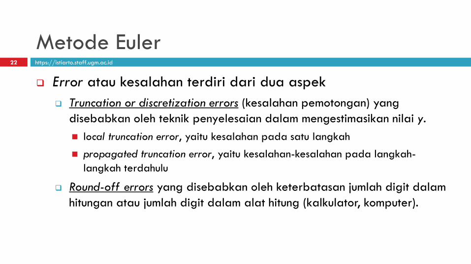
❑ Error atau kesalahan terdiri dari dua aspek

❑ Truncation or discretization errors (kesalahan pemotongan) yang

disebabkan oleh teknik penyelesaian dalam mengestimasikan nilai y.

◼ local truncation error, yaitu kesalahan pada satu langkah

◼ propagated truncation error, yaitu kesalahan-kesalahan pada langkah-

langkah terdahulu

❑ Round-off errors yang disebabkan oleh keterbatasan jumlah digit dalam

hitungan atau jumlah digit dalam alat hitung (kalkulator, komputer).


Metode Euler23

❑ Deret Taylor

( )x

yyxfy

d

d, ==

( )

nn

n

ii Rhn

yh

yhyyy +++

++=+

!...

22

1

( )( )( )

11

1!1

, ++

++

=−= n

n

nii hn

yRxxh

ξ adalah sembarang titik di antara xi dan xi+1.

Deret Taylor dapat pula dituliskan dalam bentuk lain sbb.

( )( ) ( )( ) ( )1

12

1!

,...

2

,, +

−

+ +++

++= nniin

iiiiii hOh

n

yxfh

yxfhyxfyy

O(hn+1) menyatakan bahwa local truncation error adalah proporsional terhadap selang

jarak dipangkatkan (n+1).


Metode Euler24

( )( ) ( )( ) ( )1

12

1!

,...

2

,, +

−

+ +++

++= nniin

iiiiii hOh

n

yxfh

yxfhyxfyy

Euler Error, Et

❑ true local truncation error of the Euler Method (Et)

❑ untuk selang h kecil, error mengecil seiring dengan

peningkatan tingkat

❑ error Et dapat didekati dengan Ea

( ) 2

2

,h

yxfEE iiat

= ( )2hOEa =atau


Metode Euler25

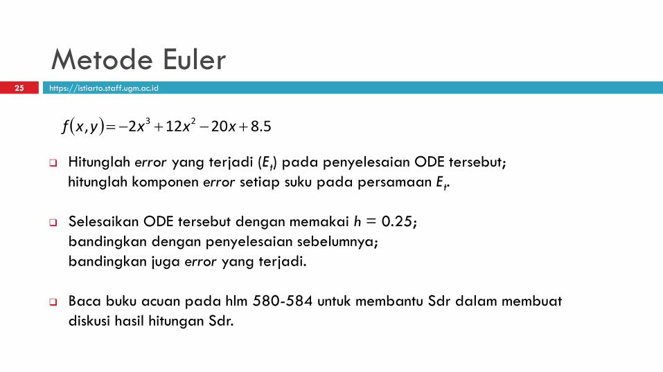
( ) 5.820122, 23 +−+−= xxxyxf

❑ Hitunglah error yang terjadi (Et) pada penyelesaian ODE tersebut;

hitunglah komponen error setiap suku pada persamaan Et.

❑ Selesaikan ODE tersebut dengan memakai h = 0.25;

bandingkan dengan penyelesaian sebelumnya;

bandingkan juga error yang terjadi.

❑ Baca buku acuan pada hlm 580-584 untuk membantu Sdr dalam membuat

diskusi hasil hitungan Sdr.


Metode Euler26

❑ Error pada Metode Euler dapat dihitung dengan memanfaatkan Deret Taylor

❑ Keterbatasan

❑ Deret Taylor hanya memberikan perkiraan/estimasi local truncation error, yaitu error yang

timbul pada satu langkah hitungan Metode Euler, bukan propagated truncation error.

❑ Hanya mudah dipakai apabila ODE berupa fungsi polinomial sederhana yang mudah

untuk di-diferensial-kan, fi(xi,yi) mudah dicari.

❑ Perbaikan Metode Euler, memperkecil error

❑ Pakailah selang h kecil.

❑ Metode Euler tidak memiliki error apabila ODE berupa fungsi linear.


Metode Heun

Penyelesaian ODE27



Metode Heun28

xi xi+1

step size = h

x

y

slope = φi

2slope

01++

= ii

slope = φ0i+1

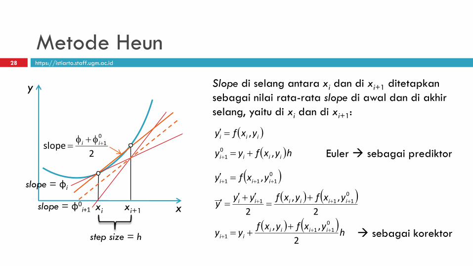
Slope di selang antara xi dan di xi+1 ditetapkan

sebagai nilai rata-rata slope di awal dan di akhir

selang, yaitu di xi dan di xi+1:

( )iii yxfy ,=

( )hyxfyy iiii ,01 +=+ Euler → sebagai prediktor

( )0111 , +++ =

iii yxfy

( ) ( )2

,,

2

0111 +++ +

=+

= iiiiii yxfyxfyyy

( ) ( )h

yxfyxfyy iiiiii

2

,, 011

1++

+

++= → sebagai korektor


Metode Heun29

❑ Pakailah Metode Heun untuk mengintegralkan ODE di bawah ini, dari x = 0

s.d. x = 4 dengan selang langkah h = 1

yex

yy x 5.04

d

d 8.0 −==

❑ Syarat awal yang diterapkan pada ODE tsb adalah bahwa pada x = 0,

y = 2

❑ Penyelesaian eksak ODE tsb yang diperoleh dari kalkulus adalah:

( ) xxx eeey 5.05.08.0 23.1

4 −− +−=


Metode Heun30

❑ Selang ke-1, dari x0 = 0 s.d. x1 = x0 + h = 1:

( ) ( ) ( ) ( ) 325.042,0, 08.000 =−== efyxf

( ) ( ) 5132, 00001 =+=+= hyxfyy

slope di titik ujung awal, (x0, y0)

prediktor y1

slope di titik ujung akhir, (x1, y1)( ) ( ) ( ) ( ) 4021637.655.045,1, 18.0011 =−== efyxf

slope rata-rata selang ke-170108185.42

4021637.63=

+=y

( ) 7010819.6170108185.4201 =+=+= hyyy korektor y1


Metode Heun31

i xi yi (eksak) f(xi,yi)awal yi (prediktor) f(xi,yi)akhir f(xi,yi)rerata yi (korektor) εt

0 0 2 3 --- --- --- 2 ---

1 1 6.1946 5.5516 5.0000 6.4022 4.7011 6.7011 -8%

2 2 14.8439 11.6522 12.2527 13.6858 9.6187 16.3198 -10%

3 3 33.6772 25.4931 27.9720 30.1067 20.8795 37.1992 -10%

4 4 75.3390 --- 62.6923 66.7840 46.1385 83.3378 -11%


Metode Heun32

0

30

60

90

0 1 2 3 4

Y

X

Eksak

Heun


Metode Heun33

❑ Metode Heun dapat diterapkan secara iteratif pada saat

menghitung slope di ujung akhir selang dan nilai yi+1

korektor

❑ nilai yi+1 korektor pertama dihitung berdasarkan nilai yi+1

prediktor

❑ nilai yi+1 korektor tersebut dipakai sebaga nilai yi+1 prediktor

❑ hitung kembali nilai yi+1 korektor yang baru

❑ ulangi kedua langkah terakhir tersebut beberapa kali

❑ Perlu dicatat bahwa

❑ error belum tentu selalu berkurang pada setiap langkah iterasi

❑ iterasi tidak selalu konvergen

( ) ( )h

yxfyxfyy iiiiii

2

,, 011

1++

+

++=

( ) ( )h

yxfyxfyy iiiiii

2

,, 011

1++

+

++=


Metode Heun34

❑ Iterasi kedua pada selang ke-1, dari x0 = 0 s.d. x1 = x0 + h = 1:

prediktor y1 = korektor y1(lama)

slope di titik ujung akhir, (x1, y1)( ) ( )( ) ( )

5516228.5

7010819.65.04

7010819.6,1,18.0

011

=

−=

=

e

fyxf

slope rata-rata selang ke-12758114.42

5516228.53=

+=y

( ) 2758114.6127581145.4201 =+=+= hyyy korektor y1

( ) 7010819.6old101 == yy

❑ Iterasi di atas dapat dilakukan beberapa kali


Metode Poligon

(Modified Euler Method)

Penyelesaian ODE35



Metode Poligon36

xi xi+1

step size = h

x

y

slope = φislope = φi+½

Slope di selang antara xi dan di xi+1 ditetapkan

sebagai nilai slope di titik tengah selang, yaitu di

xi+½:

( )iii yxfy ,=

( )2

,21

hyxfyy iiii

+=+

slope di titik awal

( )21

21

21 ,

+++=

iiiyxfy

( )hyxfyyiiii

21

21 ,1 +++ +=

slope = φi+½

xi+½

ekstrapolasi ke titik tengah

slope di titik tengah

ekstrapolasi ke titik akhir


Metode Poligon37

❑ Pakailah Metode Poligon untuk mengintegralkan ODE di bawah ini, dari x = 0

s.d. x = 4 dengan selang langkah h = 1

yex

yy x 5.04

d

d 8.0 −==

❑ Syarat awal yang diterapkan pada ODE tsb adalah bahwa pada x = 0,

y = 2

❑ Ingat penyelesaian eksak ODE tsb yang diperoleh dari kalkulus adalah:

( ) xxx eeey 5.05.08.0 23.1

4 −− +−=


Metode Poligon38

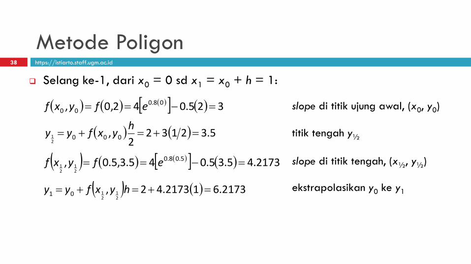
❑ Selang ke-1, dari x0 = 0 sd x1 = x0 + h = 1:

( ) ( ) ( ) ( ) 325.042,0, 08.000 =−== efyxf

( ) ( ) 5.321322

, 00021 =+=+=

hyxfyy

slope di titik ujung awal, (x0, y0)

titik tengah y½

slope di titik tengah, (x½, y½)( ) ( ) ( ) ( ) 2173.45.35.045.3,5.0, 5.08.0

21

21 =−== efyxf

ekstrapolasikan y0 ke y1( ) ( ) 2173.612173.42,21

2101 =+=+= hyxfyy


Metode Poligon39

i xi yi (eksak) f(xi,yi) xi +½ yi +½ f(xi +½,yi +½) yi εt

0 0 2 3 --- --- --- 2 ---

1 1 6.1946 5.7935 0.5 3.5000 4.2173 6.2173 -0.4%

2 2 14.8439 12.3418 1.5 9.1141 8.7234 14.9407 -0.7%

3 3 33.6772 27.1221 2.5 21.1116 19.0004 33.9412 -0.8%

4 4 75.3390 --- 3.5 47.5022 42.0275 75.9686 -0.8%


Metode Poligon40

0

30

60

90

0 1 2 3 4

Y

X

Eksak

Poligon


Metode Runge-Kutta

Penyelesaian ODE41



Metode Runge-Kutta42

❑ Metode Euler

❑ kurang teliti

❑ ketelitian lebih baik diperoleh dengan cara memakai pias kecil atau

memakai suku-suku derivatif berorde lebih tinggi pada Deret Taylor

❑ Metode Runge-Kutta

❑ lebih teliti daripada Metode Euler

❑ tanpa memerlukan suku derivatif



❑ Bentuk umum penyelesaian ODE dengan Metode Runge-Kutta adalah:

( )hhyxyy iiii ,,1 +=+

❑ Fungsi φ dapat dituliskan dalam bentuk umum sbb:

( )hyx ii ,, adalah increment function yang dapat

diinterpretasikan sebagai slope atau gradien

fungsi y pada selang antara xi s.d. xi+1

nnkakaka +++= ...2211

a adalah konstanta dan k adalah: ( )

( )

( )

( )hkqhkqhkqyhpxfk

hkqhkqyhpxfk

hkqyhpxfk

yxfk

nnnnninin

ii

ii

ii

11,122,111,11

22212123

11112

1

...,

,

,

,

−−−−−− +++++=

+++=

++=

=

setiap k saling terhubung dengan

k yang lain → k1 muncul pada

pers k2 dan k2 muncul pada pers

k3 dst.



❑ Terdapat beberapa jenis Metode Runge-Kutta yang dibedakan dari jumlah

suku pada persamaan untuk menghitung k:

❑ RK tingkat-1 (first-order RK): n = 1

❑ RK tingkat-2 (second-order RK): n = 2

❑ RK tingkat-3 (third-order RK): n = 3

❑ RK tingkat-4 (fourth-order RK): n = 4

❑ Order of magnitude kesalahan penyelesaian Metode RK tingkat n:

❑ local truncation error = O(hn+1)

❑ global truncation error = O(hn)

( )

( ) nnii

iiii

kakakahyx

hhyxyy

+++=

+=+

...,,

,,

2211

1


Second-order Runge-Kutta Method45

( )hkakayy ii 22111 ++=+ ( )

( )hkqyhpxfk

yxfk

ii

ii

11112

1

,

,

++=

=

a1, a2, p1, q11 unknowns → perlu 4 persamaan

❑ Deret Taylor

( ) ( )2

,,2

1

hyxfhyxfyy iiiiii

++=+( )

x

y

y

f

x

fyxf ii

d

d,

+

=

( )2d

d,

2

1

h

x

y

y

x

x

fhyxfyy iiii

+

++=+

❑ Bentuk umum persamaan penyelesaian ODE dengan 2nd-order RK



( ) ( ) ( )2111111112 ,, hO

y

fhkq

x

fhpyxfhkqyhpxfk iiii +

+

+=++=

❑ Bentuk di atas diterapkan pada persamaan k2

( ) ( ) ...,, +

+

+=++

y

gs

x

gryxgsyrxg

yi+1

= yi+a

1hf x

i,y

i( )+a2hf x

i,y

i( )+a2p1h2 ¶ f

¶x+a

2q11h2 f x

i,y

i( )¶ f

¶x+O h3( )

= yi+ a

1f x

i,y

i( )+a2f x

i,y

i( )éë

ùûh+ a

2p1

¶ f

¶x+a

2q11f x

i,y

i( )¶ f

¶x

é

ëê

ù

ûúh

2 +O h3( )

❑ Ingat, Deret Taylor untuk fungsi yang memiliki 2 variabel

❑ Bentuk umum penyelesaian ODE metode 2nd-order RK menjadi:



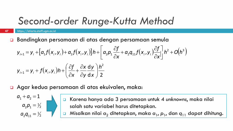
( ) ( ) ( ) ( )3211212211 ,,, hOh

x

fyxfqa

x

fpahyxfayxfayy iiiiiiii +

+

+++=+

❑ Bandingkan persamaan di atas dengan persamaan semula

❑ Agar kedua persamaan di atas ekuivalen, maka:

( )2d

d,

2

1

h

x

y

y

x

x

fhyxfyy iiii

+

++=+

21

112

21

12

21 1

=

=

=+

qa

pa

aa❑ Karena hanya ada 3 persamaan untuk 4 unknowns, maka nilai

salah satu variabel harus ditetapkan.

❑ Misalkan nilai a2 ditetapkan, maka a1, p1, dan q11 dapat dihitung.



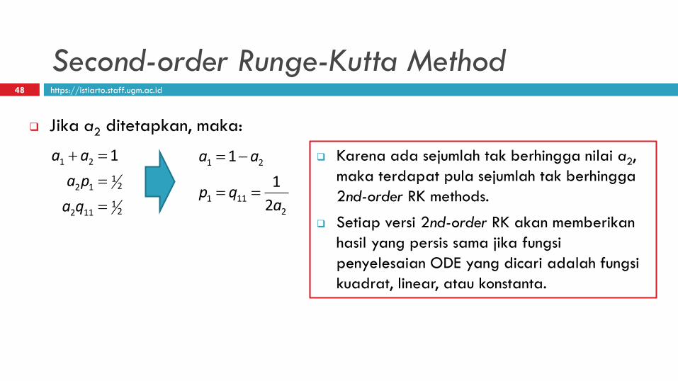
❑ Jika a2 ditetapkan, maka:

21

112

21

12

21 1

=

=

=+

qa

pa

aa

2

111

21

2

1

1

aqp

aa

==

−= ❑ Karena ada sejumlah tak berhingga nilai a2,

maka terdapat pula sejumlah tak berhingga

2nd-order RK methods.

❑ Setiap versi 2nd-order RK akan memberikan

hasil yang persis sama jika fungsi

penyelesaian ODE yang dicari adalah fungsi

kuadrat, linear, atau konstanta.



❑ Metode Heun dengan korektor tunggal

❑ Metode poligon yang diperbaiki (improved polygon method)

❑ Metode Ralston

1, 11121

121

2 ==== qpaa ( )hkkyy ii 221

121

1 ++=+

21

11112 ,01 ==== qpaa

( )

( )12

1

,

,

hkyhxfk

yxfk

ii

ii

++=

=

( )hkkyy ii 232

131

1 ++=+

hkyy ii 21 +=+ ( )

( )121

21

2

1

,

,

hkyhxfk

yxfk

ii

ii

++=

=

43

11131

132

2 , ==== qpaa ( )

( )143

43

2

1

,

,

hkyhxfk

yxfk

ii

ii

++=

=



❑ Pakailah berbagai 2nd-order RK methods untuk mengintegralkan ODE di

bawah ini, dari x = 0 s.d. x = 4 dengan selang langkah h = 0.5:

( ) 5.820122d

d, 23 +−+−== xxx

x

yyxf

❑ Syarat awal yang diterapkan pada ODE tsb adalah bahwa di titik x= 0,

y = 1

❑ Bandingkan hasil-hasil penyelesaian dengan berbagai metode RK tsb.



Single-corrector Heun

i xi yi (eksak) k1 k2 φ yi εt0 0 1 8.5 1.25 4.875 1 0.0%

1 0.5 3.21875 1.25 -1.5 -0.125 3.4375 -6.8%

2 1 3 -1.5 -1.25 -1.375 3.375 -12.5%

3 1.5 2.21875 -1.25 0.5 -0.375 2.6875 -21.1%

4 2 2 0.5 2.25 1.375 2.5 -25.0%

5 2.5 2.71875 2.25 2.5 2.375 3.1875 -17.2%

6 3 4 2.5 -0.25 1.125 4.375 -9.4%

7 3.5 4.71875 -0.25 -7.5 -3.875 4.9375 -4.6%

8 4 3 --- --- --- 3 0.0%



Improved Polygon


1 0.5 3.21875 1.25 -0.59375 -0.59375 3.109375 3.4%

2 1 3 -1.5 -1.65625 -1.65625 2.8125 6.3%

3 1.5 2.21875 -1.25 -0.46875 -0.46875 1.984375 10.6%

4 2 2 0.5 1.46875 1.46875 1.75 12.5%

5 2.5 2.71875 2.25 2.65625 2.65625 2.484375 8.6%

6 3 4 2.5 1.59375 1.59375 3.8125 4.7%

7 3.5 4.71875 -0.25 -3.21875 -3.21875 4.609375 2.3%

8 4 3 --- --- --- 3 0.0%



Second-order Ralston Runge-Kutta


1 0.5 3.21875 1.25 -1.15234 -0.35156 3.277344 -1.8%

2 1 3 -1.5 -1.51172 -1.50781 3.101563 -3.4%

3 1.5 2.21875 -1.25 0.003906 -0.41406 2.347656 -5.8%

4 2 2 0.5 1.894531 1.429688 2.140625 -7.0%

5 2.5 2.71875 2.25 2.660156 2.523438 2.855469 -5.0%

6 3 4 2.5 0.800781 1.367188 4.117188 -2.9%

7 3.5 4.71875 -0.25 -5.18359 -3.53906 4.800781 -1.7%

8 4 3 --- --- --- 3.03125 -1.0%



0

2

4

6

0 1 2 3 4

Exact

Heun

Improved Polygon

Ralston

X

Y


Third-order Runge-Kutta Method55

❑ Persamaan penyelesaian ODE 3rd-order RK methods:

❑ Catatan:

❑ Jika derivatif berupa fungsi x saja, maka 3rd-order RK sama dengan

persamaan Metode Simpson ⅓

( ) hkkkyy ii 32161

1 4 +++=+( )

( )( )213

121

21

2

1

2,

,

,

hkhkyhxfk

hkyhxfk

yxfk

ii

ii

ii

+−+=

++=

=


Third-order Runge-Kutta Method56

Third-order Runge-Kutta

i xi yi (eksak) k1 k2 k3 φ yi εt0 0 1 8.5 4.219 1.25 4.438 1 0.0%

1 0.5 3.21875 1.25 -0.594 -1.5 -0.438 3.21875 0.0%

2 1 3 -1.5 -1.656 -1.25 -1.563 3 0.0%

3 1.5 2.21875 -1.25 -0.469 0.5 -0.438 2.21875 0.0%

4 2 2 0.5 1.469 2.25 1.438 2 0.0%

5 2.5 2.71875 2.25 2.656 2.5 2.563 2.71875 0.0%

6 3 4 2.5 1.594 -0.25 1.438 4 0.0%

7 3.5 4.71875 -0.25 -3.219 -7.5 -3.438 4.71875 0.0%

8 4 3 --- --- --- --- 3 0.0%


Fourth-order Runge-Kutta Method57

❑ Persamaan penyelesaian ODE 4th-order RK methods:

❑ Catatan:

❑ Jika derivatif berupa fungsi x saja, maka 4th-order RK sama dengan

persamaan Metode Simpson ⅓

( ) hkkkkyy ii 432161

1 22 ++++=+( )

( )

( )( )34

221

21

3

121

21

2

1

,

,

,

,

hkyhxfk

hkyhxfk

hkyhxfk

yxfk

ii

ii

ii

ii

++=

++=

++=

=


Fourth-order Runge-Kutta Method58

Fourth-order Runge-Kutta

i xi yi (eksak) k1 k2 k3 k4 φ yi εt0 0 1 8.5 4.219 4.219 1.25 4.44 1 0.0%

1 0.5 3.21875 1.25 -0.594 -0.594 -1.5 -0.44 3.21875 0.0%

2 1 3 -1.5 -1.656 -1.656 -1.25 -1.56 3 0.0%

3 1.5 2.21875 -1.25 -0.469 -0.469 0.5 -0.44 2.21875 0.0%

4 2 2 0.5 1.469 1.469 2.25 1.44 2 0.0%

5 2.5 2.71875 2.25 2.656 2.656 2.5 2.56 2.71875 0.0%

6 3 4 2.5 1.594 1.594 -0.25 1.44 4 0.0%

7 3.5 4.71875 -0.25 -3.219 -3.219 -7.5 -3.44 4.71875 0.0%

8 4 3 --- --- --- --- --- 3 0.0%


3rd- and 4th-order Runge-Kutta Methods59

❑ Pakailah 3rd-order dan 4th-order RK methods untuk mengintegralkan ODE di

bawah ini, dari x = 0 s.d. x = 4 dengan selang langkah h = 0.5:

( ) 5.820122d

d, 23 +−+−== xxx

x

yyxf

▪ Syarat awal yang diterapkan pada ODE tsb adalah bahwa di titik x = 0,

y = 1


3rd- and 4th-order Runge-Kutta Methods60

Node Exact Solution Third-order RK Fourth-order RK

i xi yi yi εt yi εt0 0 1 1 0.0% 1 0.0%

1 0.5 3.21875 3.21875 0.0% 3.21875 0.0%

2 1 3 3 0.0% 3 0.0%

3 1.5 2.21875 2.21875 0.0% 2.21875 0.0%

4 2 2 2 0.0% 2 0.0%

5 2.5 2.71875 2.71875 0.0% 2.71875 0.0%

6 3 4 4 0.0% 4 0.0%

7 3.5 4.71875 4.71875 0.0% 4.71875 0.0%

8 4 3 3 0.0% 3 0.0%

http://istiarto.staff.ugm.ac.id61

persamaan diferensial biasa - istiarto.staff.ugm.ac.id persamaan diferensial biasa.pdf · persamaan...

Documents