WORKING PAPER SERIES

Pessimistic Beliefs under Rational Learning: Quantitative Implications for the Equity Premium Puzzle

Massimo Guidolin

Working Paper 2005-005A http://research.stlouisfed.org/wp/2005/2005-005.pdf

January 2005

FEDERAL RESERVE BANK OF ST. LOUIS Research Division 411 Locust Street

St. Louis, MO 63102 ______________________________________________________________________________________

The views expressed are those of the individual authors and do not necessarily reflect official positions of the Federal Reserve Bank of St. Louis, the Federal Reserve System, or the Board of Governors.

Federal Reserve Bank of St. Louis Working Papers are preliminary materials circulated to stimulate discussion and critical comment. References in publications to Federal Reserve Bank of St. Louis Working Papers (other than an acknowledgment that the writer has had access to unpublished material) should be cleared with the author or authors.

Photo courtesy of The Gateway Arch, St. Louis, MO. www.gatewayarch.com

Pessimistic Beliefs under Rational Learning: Quantitative

Implications for the Equity Premium Puzzle.∗

Massimo GUIDOLIN�

University of Virginia

July 27, 2004

Abstract

In the presence of infrequent but observable structural breaks, we show that a model in which the

representative agent is on a rational learning path concerning the real consumption growth process can

generate high equity premia and low risk-free interest rates. In fact, when the model is calibrated to

U.S. consumption growth data, average risk premia and bond yields similar to those displayed by post-

depression (1938-1999) U.S. historical experience are generated for low levels of risk aversion. Even

ruling out pessimistic beliefs, recursive learning inßates the equity premium without requiring a strong

curvature of the utility function. Simulations reveal that other moments of equilibrium asset returns are

easily matched, chießy excess volatility and the presence of ARCH effects. These Þndings are robust to

a number of details of the simulation experiments, such as the number and dating of the breaks.

JEL codes: G12, D83.

∗I am indebted to Allan Timmermann for many useful comments. I also wish to thank seminar participants at the European

Economic Association meetings in Stockholm (August 2003), the European Financial Management Association in Basel (July

2004), the Midwest Economics Association Meetings in St. Louis (March 2003), IGIER Milan, University of Virginia, and the

Third Workshop in Macroeconomic Dynamics in Milan (December 2003). Parts of this paper have previously circulated under

the title �High Equity Premia and Crash Fears. Rational Foundations�.�Department of Economics, University of Virginia, Charlottesville - 118 Rouss Hall, Charlottesville, VA 22904-4182. Tel:

(434) 924-7654; Fax: (434) 982-2904; e-mail: mg8g@virginia.edu

1. Introduction

The bull equity markets of the 1990�s have left us with a secular (1890-1999) average 7 percent equity

return in excess of risk-free bonds.1 These Þgures are even more striking considering that over two periods

− 1930-1942 (Great Depression and WWII) and 1974-1981 (oil shocks) − average excess equity returns

have been negative (−0.41% and −1.20%). In an economy populated by risk-averse individuals, negativeexcess returns are as difficult to understand as high averages. This paper shows that high and variable

equity premia and low interest rates can all be rationalized in a simple general equilibrium model in which

agents are on a recursive, rational learning path.

Since Mehra and Prescott (1985, MP), we know that a Lucas (1978) economy with power, time-additive

expected utility, complete markets, no frictions, and in which a representative agent forms rational expecta-

tions on the only source of risk (real consumption) cannot pass the test of reproducing the historical mean

equity risk premium. This impasse is labeled the equity premium puzzle. Moreover, in MP�s framework

high risk aversion implies an implausibly low elasticity of intertemporal substitution that forces the real

riskless rate to levels in excess of historical averages, the risk-free rate puzzle (cf. Weil (1989)).

A vast literature has developed after MP had Þrst pointed out the puzzle.2 Many papers have focused

on the role of power, time-additive, expected utility preferences which constrain the elasticity of intertem-

poral substitution to be the inverse of the coefficient of relative risk-aversion (e.g. Constantinides (1990),

Campbell and Cochrane (1999), Epstein and Zin (1989)). Efforts have been directed at removing the

assumption of market completeness, showing that the additional uncertainty in individual consumption

due to the absence of insurance markets for some states helps increasing the equity premium and lowers

the risk-free rate (e.g. Constantinides and Duffie (1995)). Another strand of literature has assessed the

importance of borrowing constraints and transaction costs (Aiyagari and Gertler (1991)).

Surprisingly, less attention has been given to the mechanism by which beliefs are formed and updated.

The early literature had in fact assumed full-information rational expectations as a way to close the model

and impose some − arbitrary − consistency on the mechanism by which beliefs are formed. This means

that agents are empowered with complete knowledge of the stochastic process driving the relevant state

variables (fundamentals) and escape any kind of parameter uncertainty and the need of (econometric)

learning. Yet, besides that its level is high, we know two additional facts concerning excess returns on US

equities. First, excess returns are subject to remarkable ßuctuations. Second, high excess returns seem to

be a phenomenon of the XXth century, in particular of the 1950s and 90s. Interestingly, recent empirical

research has showed that both the 1930s and the early 1980s imply the presence of structural breaks in

the regime followed by fundamentals (Stock and Watson (1996)). Therefore it appears that changes in the

regime characterizing fundamentals tend to be followed by high equity premia, so there might be something

special about the historical path followed by the US economy.

A few papers have tried to offer explanations of the puzzles that move from events unique to the

US history, particularly the Great Depression. Rietz (1988) shows that biasing agents� beliefs to reßect

catastrophic scenarios not present in the historical data, a sizeable equity premium can be generated

1A few recent papers have shown that the realized mean excess return is likely to be an upward biased estimate of the

ex-ante, equity premium expected by investors, e.g. Pastor and Stambaugh (2000) and Fama and French (2001). These studies

estimate an equity premium in the range 3-5%.2Cochrane (2001), Kocherlakota (1996), and Mehra and Prescott (2003) survey the literature.

2

for reasonable degrees of risk aversion. However the crash state needed to deliver the result must be

truly catastrophic (Mehra and Prescott (1988)). Also, matching the empirical volatility of excess returns

remains difficult (Salyer (1998)). Danthine and Donaldson (1999) explore the same concept, showing that

Peso problems have more dramatic effects in artiÞcial samples in which economy crashes are not actually

present. Cecchetti, Lam, and Mark (2000) study the effects of belief distortions on asset prices. Under the

assumption that the rate of growth of fundamentals follows a two-state Markov switching process, they show

that some degree of pessimism relative to the maximum-likelihood estimates generates plausible moments.

However the origin of such pessimistic fears is unclear. This literature therefore relies on deviations between

realized and subjectively perceived beliefs, often in arbitrary ways. On the opposite, we are interested

in detecting situations in which rational pessimism and crash fears may arise as a consequence of the

application of simple but optimal maximum likelihood methods.

Abel (2002) explores the effects of pessimism and doubt for equilibrium asset prices. He shows that

pessimism reduces the risk-free rate and that a peculiar kind of pessimism (uniform) also increases the

average equity premium; doubt has similar effects. This makes it possible to generate plausible risk premia

for acceptable degrees of curvature of the utility function, without running into a risk-free rate puzzle. On

the other hand, Abel�s analysis is admittedly exploratory, in the sense that the sources of pessimism and

doubt are left unspeciÞed.3 Our paper may be read as an attempt to endogenously generate pessimism and

doubt when agents cannot form full information rational expectations, but recursively update an estimate

of the distribution of future growth rates.

When agents lack full information on some parameters characterizing the environment, their subjective

beliefs may rationally deviate from the empirical distribution of the state variables, without the need of

postulating in an ad-hoc fashion that markets agree on the possibility of some disaster state. A few papers

have studied the implications of recursive learning for asset pricing.4 However the implications for the

equity premium are not pursued. An exception is Brennan and Xia (2001): In a continuous-time general

equilibrium setting a representative agent recursively estimates the unobservable drift of dividends. Using

a risk aversion coefficient of 15 and a rate of time preference of -10%, they derive an equity premium

of 6 percent and a risk-free rate of 2.5 percent; the same parameters imply volatile stock returns and

realistic correlations between dividend growth and stock returns. Unfortunately, a risk aversion of 15

is high according to the literature standards and Brennan and Xia observe (p. 266) that the effects

of recursive learning are of second-order magnitude, their assumption on the randomness of the drift

parameter accounting for most of the effects. We show instead that Þrst-order effects can be obtained

from learning using a plausible degree of curvature of the utility function. Finally, Guidolin (2003) shows

that in principle at least, rational learning and pessimism may inßate the equilibrium equity premium and

lower the riskless interest rate, but he stops short of a full assessment of the quantitative implications of

the model through a standard calibration exercise.

The paper pursues three objectives. First, it removes the assumption of full-information (FI) rational

expectations with complete knowledge of the process of the risk factors. In particular, we focus on a

restrictive learning mechanism that does not allow any expected gains from implementing trading strategies

based on the impact on equilibrium prices of the future unfolding of parameter uncertainty. Such learning

3He writes that �(...) the next challenge is to explain why pessimism and doubt may occur.� (p. 1091). We contend that

departures from rationality are not necessary, while departures from complete information are.4See Barsky and De Long (1993), Bullard and Duffie (2001), Veronesi (1999), and Timmermann (1993, 2001).

3

schemes are called rational and in asset pricing applications they imply that prices reßect all possible,

future perceived distributions of the parameters� estimates (future learning).5 Second, we prove that when

a representative agent is on a learning path and the process for dividends is described by a binomial lattice

calibrated on US real consumption growth, both average excess equity returns and bond yields similar

to those displayed the by the post-depression (1934-1999) US data may be generated for low levels of

risk aversion. Third, we show that on a recursive learning path, US investors might have rationally come

to attach positive probability to crash states as a consequence of the pessimism caused by the two deep

recessions of the 1930s and 1970s. This �Peso problem� situation would have arisen in an entirely rational

and endogenous fashion. In a sense, we impose structure on the thought that

�(...) the experience of the Great Depression continues to have a signiÞcant inßuence on the

behaviour of those who experienced it directly or indirectly, even though it has not occurred in

sixty-Þve years.� (Danthine and Donaldson (1999), p. 608)

by using the Great Depression and the two oil shocks as starting points in setting the initial beliefs held by

agents on a recursive learning path. In this sense, rational learning and irrational crash fears are shown

to be observationally equivalent, although only learning provides a foundation for the persistence and size

of the belief distortions needed to rationalize observed asset prices.

The paper has the following structure. Section 2 presents a few empirical regularities. Section 3

introduces the model. Section 4 characterizes equilibrium asset prices under full-information rational

expectations. This can be considered a version of MP�s results, specialized to the case of an i.i.d. binomial

tree. Section 5 characterizes the rational learning scheme, and derives equilibrium expressions for asset

prices. Section 6 discusses the implications for the equity premium and the risk-free rate of the two

assumptions on beliefs. The FI case is shown to display non-trivial equilibrium properties that may prevent

the generation of high equity premia even for high levels of risk-aversion. Section 6 goes on to show how

rational learning might contribute to solve the puzzles. Section 7 conducts simulation experiments. Section

8 discusses the role of initial beliefs and performs a few additional robustness checks. Section 9 concludes.

2. Stylized Facts

We use the same annual data as Shiller (1990), appropriately extended to cover the 110 years of the period

1890-1999. Stock prices and dividends correspond to January levels of the Standard & Poors Composite

Indices. Real stock prices and dividends are obtained by dividing the series by the consumption deßator

series (non-durables and services). The risk-free rate corresponds to the return of a strategy that rolls

over an investment of one dollar in 4-6 months commercial paper. The real risk-free rate is calculated by

subtracting the annual inßation rate (calculated as the percentage change of the consumption deßator)

from the nominal rate. The per capita consumption growth rate series concerns non-durables and services.

2.1. Facts Concerning the Real Consumption Growth Rate

Real consumption growth data conÞrm their well-known �smoothness�. The average growth rate is 1.80%

per year (identical to MP) and the standard deviation is 3.27% (lower than MP�s 3.57%). The series

5Guidolin and Timmermann (2003b) show these learning schemes can be equivalently characterized as Bayesian learning

mechanisms when some assumptions on prior beliefs are made.

4

exhibits a low degree of serial correlation (-0.15), which matches the Þgure in MP. Hence the growth of the

endowment process is well approximated by an i.i.d. process. The volatility of real consumption growth

substantially decreases after WWII, from 4.4% over 1890-1945 to 1.4% over 1946-1999.

Such changes in the consumption process open the possibility that fundamentals be subject to structural

breaks. In particular, breaks may have been so evident to be perceived by US investors. Chu, Stinchcombe,

and White (1996) develop a procedure of real time, recursive monitoring of structural changes in regression

models. The real time nature of the algorithm allows us to locate (i.e. test for) structural breaks perceived

by the agents as they were receiving new data and making decisions. Consider the following autoregressive

process for gt, the rate of growth of real consumption

gt ≡ ct − ct−1ct−1

= µ+LXj=1

φjLjgt + ²t = x

0tθt + ²t,

where ct is real per-capita consumption, L is the standard lag operator, and ²t a white noise process. Call

ι the minimum time span over which the parameters θt ≡ [µt φ1t ... φLt]0 are assumed to remain constant,i.e. θτ+1 = θτ+2 = ... = θτ+ι, where τ is the time of the last structural break detected by agents and

xt ≡ [1 gt−1 ... gt−L]0. Suppose agents aim at testing the presence of a break in the regression model at

time t > τ + ι. Chu et al. suggest calculating the following �ßuctuation detector�:

�Ft = (t− τ) �D−1/2ι (�θt − �θι). (1)

Details on the structure of the test statistic and on the associated asymptotic bounds under the null of no

breaks are provided in Appendix A. In practice, we can think that after at least ι observations have been

received after a break in τ , the agents start the recursive calculation of �Ft. If at t̄ the statistic hits the

bounds, then the null of no structural breaks since τ fails to be rejected. t̄ becomes then the time of the

new structural break. After ι further observations have been received, agents start again monitoring the

occurrence of breaks, etc. We apply these tests to:

gt = µ+ φgt−1 + ²t,

a standard AR(1) model (Timmermann (2001)). We use a value ι = 20 exceeding the average duration of

US business cycles to prevent natural ßuctuations to be interpreted as breaks. Figure 1 shows the results

of tests based on the ßuctuation detector (1) by plotting | �F (µ)t | and | �F (β)t | vs. the asymptotic bound at1 percent test size. The null of no break is unequivocally rejected for both µ and β in correspondence to

the mid 1930s, the Great Depression. Indeed the mean level of �µ jumps from 3% to 2% in the mid 1930s,

while the mean �β goes from about -0.45 to -0.2; this implies a reduction in the perceived long run mean

consumption growth from 2.07% to 1.67% that Þts the negative real growth during 1929-1938 (-0.66%).

The middle plots of Figure 1 repeat the analysis conditioning on the occurrence of a Þrst structural

break during the 1930s: the analysis is applied to a shorter annual data set covering the 1938-1999 period.

Although the evidence on a further break in µ is inconclusive, the ßuctuation detector for β locates a second

break in the early 1980s, in the aftermath of the oil shocks. Indeed in the period 1974-1982 the average

real growth rate was 1.67%, below the 2.10% average of 1939-1973. These econometric tests suggest the

presence of two structural breaks in the fundamentals� process: the Þrst in 1938, at the conclusion of the

Depression cycle, and the second in 1982, at the conclusion of the two cycles marked by the oil price shocks.

5

2.2. Facts Concerning Asset Returns

Over 1938-1999 the mean excess return on stocks has been 7.64%, above MP�s 6.18%. We take this long-run

average as a measure of the ex-post equity premium. On the other hand, the average level of the risk-free

rate, 0.96%, is similar to the 0.80% calculated by MP. The volatility of the equity premium is 16% while the

risk-free rate is stable, 3.86%. Notoriously, a high volatility of excess equity returns along with a negligible

standard deviation for the risk-free rate is puzzling (Hagiwara and Herce (1997)) and has proven to be

a tough stylized fact to match (Cecchetti, Lam, and Mark (1990)). During the period following the oil

shocks, the equity premium climbs even higher (10.36%) despite the higher average risk-free rate (3.84%).

The volatility of both interest rates and the equity premium declines to.14.42% and 1.98%, respectively.

3. The Model

The model is a version of the inÞnite horizon, representative agent, endowment economy studied by MP

(1985). There are two assets: a one-period, risk-free, zero coupon bond in endogenous zero net supply,

yielding an interest rate of rt (hence Bt =1

1+rtwhere B is the bond price), and a stock index with price St

in exogenous net unit supply. The stock pays an inÞnite stream of real dividends {Dt}∞t=1 . These dividendsare perishable, they cannot be reinvested and therefore they must be consumed in the period they are

received. The initial level of fundamentals D0 is given. The real growth rate of dividends gt ≡ DtDt−1 − 1

follows a two-state Markov chain. State 1 is characterized by a high growth rate gh and can be identiÞed

with business cycle expansions, while state 2 is a recession state in which growth is −1 < gl < 0 < gh:

During a recession fundamentals decrease. The transition matrix is

Π =

"p 1− p

1− q q

#

with stationary probabilitiesh1−q2−p−q ,

1−p2−p−q

iand Þrst-order autocorrelation p+ q − 1.

When p = 1 − q = 1 − π, the probability of switching to a given state becomes independent of theoriginal state, the stationary probabilities of the two states reduce to {π, 1− π} , and the Þrst-order serialcorrelation is nil. When confronted with smooth processes such as US consumption growth, a zero Þrst-

order autocorrelation is realistic.6 In this case, the driving process for the endowment is a binomial tree.

Also, gh, gl, and π may be subject to infrequent jumps, i.e. structural breaks. For simplicity, assume that

structural breaks are observable. Events of the magnitude of the Great Depression and the world energy

crises are likely to be rapidly recognized because of their deep consequences. Thus, between today and a

certain future date T and conditioning on no structural breaks occurring, the continuously compounded

rate of growth of dividends follows a (T − t)-steps binomial process by which the dividend growth rate ineach period [t, t+ 1] can be either gh with probability π or gl with probability 1− π:

gt =

(gh with prob. π

gl with prob. 1− π ∀t ≥ 1, π ∈ (0, 1) (2)

and the rates of growth over time are independent. The description of the physical environment is completed

by the assumption of perfect capital markets: unlimited short sales possibilities, perfect liquidity, no taxes,

6Abel (2002) and Barsky and De Long (1993) stress that to a Þrst approximation dividends follow a random walk.

6

transaction fees, bid-ask spreads, markets are open at all points in time in which news on dividends are

generated, no borrowing or lending constraints.

There exists a representative agent who has power, constant relative risk aversion preferences

u(ct) =

½C1−γt −11−γ γ 6= 1

lnCt γ = 1(3)

where Ct is real consumption. The agent maximizes the discounted value (at a rate ρ > 0) of the inÞnite

stream of expected future (instantaneous) utilities deriving from consumption of real dividends.

4. Asset Pricing Under Full Information Rational Expectations

Assume the representative agent knows the stochastic process of dividends, i.e. its binomial structure,

the parameters {gh, gl,πt} , and that she forms rational expectations. Moreover, assume that breaks occurwith such a low frequency to be safely disregarded by agents when they form expectations on future cash

ßows and determine current asset prices.7 The representative agent solves:

max{Ct+k,wst+k,wbt+k}∞k=0

E

" ∞Xk=0

βku(Ct+k)|zt#

s.t. Ct+k + wst+kSt+k + w

bt+kBt+k = w

st+k−1(St+k +Dt+k) + w

bt+k−1, (4)

where β = 11+ρ , and w

st+k, w

bt+k represent the number of shares of stocks and bonds in the agent�s portfolio

as of period t + k. E [·|zt] ≡ Et[·] denotes the conditional expectation operator measurable with respectto zt, the information set. Standard dynamic programming methods yield the following Euler equations:

St = E [Qt+1(St+1 +Dt+1) | zt] (5)

Bt = E [Qt+1 | zt] , (6)

where Qt+1 = βu0(Ct+1)u0(Ct) = β

³Ct+1Ct

´−γis the pricing kernel (stochastic discount factor) deÞned as the prod-

uct of the subjective discount factor and the intertemporal marginal rate of substitution in consumption.

In equilibrium dividends are the only source of endowment and consumption, so Ct+k = Dt+k ∀k ≥ 0.In the full information case, a solution for asset prices can easily be obtained using the method of

undetermined coefficients. It is straightforward to prove that the full information rational expectations

(FI) stock price, SFIt , is given by

SFIt = limT→∞

Et

TXj=1

Ãβj

jYi=1

(Dt+i/Dt+i−1)1−γ! ·Dt. (7)

The linear homogenous form of the pricing function SFIt = ΨFIt Dt is a direct implication of expected utility

maximization, where ΨFIt denotes the pricing kernel, i.e. the price-dividend ratio, see Abel (2002, p. 1079)

and Brennan and Xia (2001, p. 258), a time-varying function of πt. Assuming

ρ > πtg∗h + (1− πt)g∗l , (8)

7Our empirical analysis has isolated only 2 breaks in a 110 years long time series, a frequency of 1.8%. Timmermann (2001)

uses a monthly probability of 0.3%. Guidolin (2003) calculates by simulation equilibrium prices when future, random breaks

are taken into account and concludes that closed-form solutions provide a good approximation.

7

where g∗l ≡ (1 + gl)1−γ − 1 and g∗h ≡ (1 + gh)1−γ − 1, Guidolin and Timmermann (2003a,b) prove that

SFIt = ΨFIt Dt =1 + g∗l + πt(g

∗h − g∗l )

ρ− g∗l − πt(g∗h − g∗l )Dt, (9)

while the positive, time-invariant equilibrium risk-free rate, rf,FI , is

rf,FI =1

BFI− 1 = 1 + ρ

(1 + gl)−γ + πt [(1 + gh)−γ − (1 + gl)−γ] − 1. (10)

Since the stock price is homogeneous of degree one in dividends, it follows the same binomial tree {gh, gl,π}as dividends. Condition (8) ensures not onlyΨFIt > 0 but also convergence of the series

P∞s=1Et[(

Qsk=1Qt+k)

Dt+s] and existence of the equilibrium. For ρ > 0 and given {gh, gl,π}, too low or too high levels of γ

might violate this condition, meaning that there exists no Þnite stock price such that markets clear. When

γ is too low for (8) to hold, then γ must be close to zero. A γ ' 0 means that the agent is nearly

risk-neutral so that πtg∗h + (1 − πt)g∗l ' E[gt] and from (10) rFI ' ρ. Then condition (8) is equivalent

to rFI > E[gt] since a risk-neutral agent will never demand risk-free bonds when it is possible to earn

a higher expected stream of cash dividends from holding the stock. No equilibrium exists as the stock

price diverges to inÞnity in response to the excess demand while the bond price falls to zero as all agents

would like to issue bonds to Þnance their stock holdings. A high γ can prevent satisfaction of (8) since

when gl ≤ 0 there exists a state in which the agent�s intertemporal marginal rate of substitution (IMRS)u0(Dt+k)/u0(Dt+k−1)|gt+k=gl = (1 + gl)

−γ diverges as γ → ∞. This means that all assets paying out apositive amount of real consumption in the bad state receive an inÞnite valuation.

5. Asset Prices on a Learning Path

5.1. Rational Learning

Suppose instead that the representative agent is on a learning path: he knows that dividends follow a

binomial lattice {gh, gl,πt}. He also knows gh and gl. However, πt is unknown and the agent estimatesit using all the available information since its last change (break), time τ b. The agent recursively gains

knowledge on πt by using the simple frequency estimator:

bπτbt =nτb0 +

Ptj=τb+1

I{gj=gh}N τb0 + t− τ b + 1 =

nτb0 + nτbt

N τb0 +N τb

t

t > τ b, (11)

where I{gt+j=gh} takes value 1 when at step/time j of the binomial tree dividends grow at a high rate, andzero otherwise. nτbt denotes the number of high growth states recorded between τ b+1 and time t, while N

τbt

is the total number of dividend movements recorded over [τ b + 1, t]. After a break, investors are assumed

to start out with beliefs synthesized by {nτb0 , N τb0 }.8 bπτb0 = nτb0 /N

τb0 reßects a starting belief agents hold on

the probability of a good state, with 1/N τb0 the associated degree of precision. As stressed by Timmermann

(2001, p. 305), the presence of infrequent breaks makes learning a much more plausible assumption than

full information rational expectations as investors rarely will have available a large historical sample from

which to derive precise estimates of the relevant parameters.

8If breaks are observable, agents know with certainty when to restart their learning process and discard information from

the previous regime. On the other hand, if agents were uncertain as to the occurrence of breaks, explicit econometric methods

to estimate the likelihood of a break at all times τ ≤ t should be used. We do not pursue this extension here.

8

Agents are on a rational learning (RL) path, see Guidolin and Timmermann (2003b), i.e. they take into

account that their beliefs on π will be updated for t0 > t and incorporate the effects of future learning intheir current beliefs.9 Consider the state vector Wt with stationary density parameterized by θ ∈ Θ ⊆ <p,f(Wt; θ). Suppose an agent wants to calculate a T -steps ahead forecast W

ft+T . If the agent does not know

π but he is on a RL path, then his best forecast will be:

W ft+T = E

n...E

hE³Wt+T |zt+T−1,bθt+T−1´ |zt+T−2,bθt+T−2i ...|zt,bθto . (12)

E³·|zt+k,bθt+k´ is a conditional expectation measurable with respect to the information structure zt+k,

conditional on current knowledge on θ, some estimator bθt+k. (12) shows that the agent takes into accountthat her knowledge about θ will change for t0 > t with probability 1. The sequence {bθt,bθt+1, ...,bθt+T−1}enters the forecasting problem and future beliefs are recognized to be state-dependent.

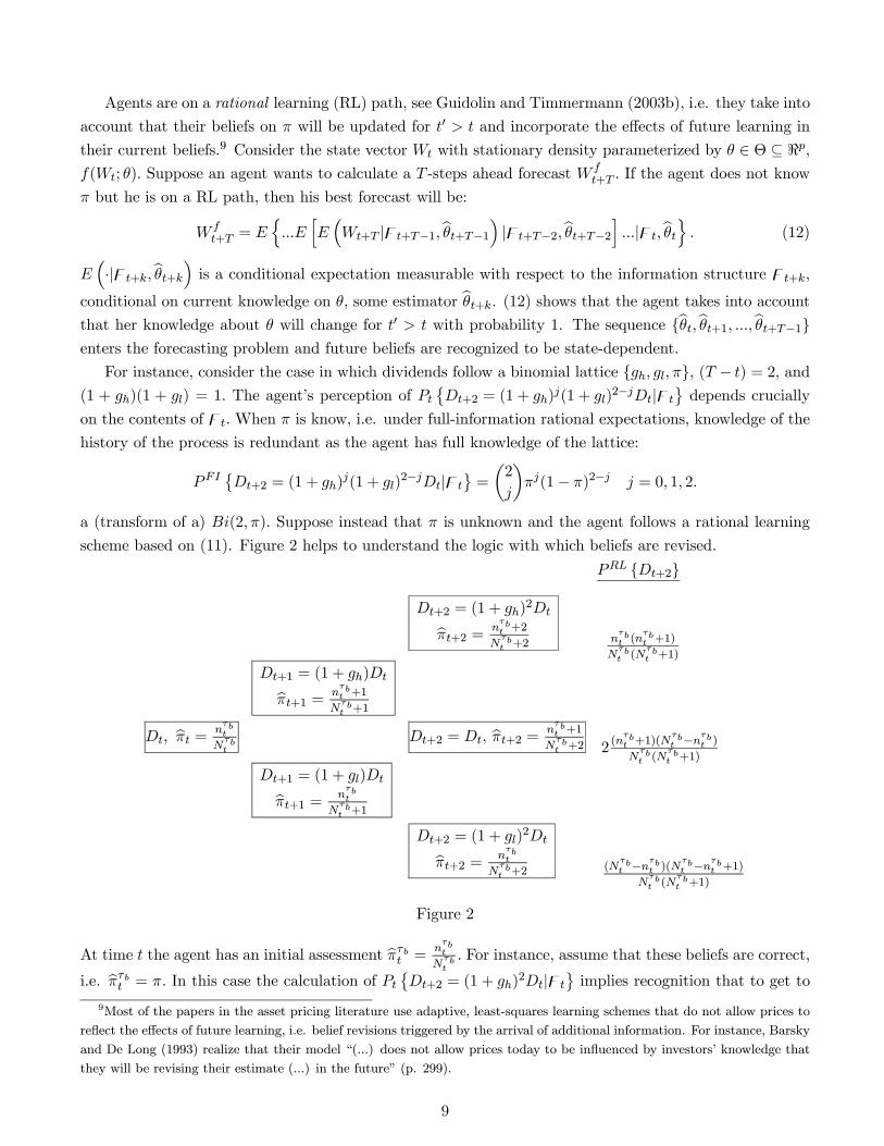
For instance, consider the case in which dividends follow a binomial lattice {gh, gl,π}, (T − t) = 2, and(1 + gh)(1 + gl) = 1. The agent�s perception of Pt

©Dt+2 = (1 + gh)

j(1 + gl)2−jDt|zt

ªdepends crucially

on the contents of zt.When π is know, i.e. under full-information rational expectations, knowledge of thehistory of the process is redundant as the agent has full knowledge of the lattice:

PFI©Dt+2 = (1 + gh)

j(1 + gl)2−jDt|zt

ª=

µ2

j

¶πj(1− π)2−j j = 0, 1, 2.

a (transform of a) Bi(2,π). Suppose instead that π is unknown and the agent follows a rational learning

scheme based on (11). Figure 2 helps to understand the logic with which beliefs are revised.

PRL {Dt+2}

Dt+2 = (1 + gh)2Dtbπt+2 = n

τbt +2

Nτbt +2 n

τbt (n

τbt +1)

Nτbt (N

τbt +1)

Dt+1 = (1 + gh)Dtbπt+1 = nτbt +1

Nτbt +1

Dt, bπt = nτbt

Nτbt

Dt+2 = Dt, bπt+2 = nτbt +1

Nτbt +2 2

(nτbt +1)(N

τbt −nτbt )

Nτbt (N

τbt +1)

Dt+1 = (1 + gl)Dtbπt+1 = nτbt

Nτbt +1

Dt+2 = (1 + gl)2Dtbπt+2 = n

τbt

Nτbt +2 (N

τbt −nτbt )(N

τbt −nτbt +1)

Nτbt (N

τbt +1)

Figure 2

At time t the agent has an initial assessment bπτbt =nτbt

Nτbt

. For instance, assume that these beliefs are correct,

i.e. bπτbt = π. In this case the calculation of Pt©Dt+2 = (1 + gh)

2Dt|ztªimplies recognition that to get to

9Most of the papers in the asset pricing literature use adaptive, least-squares learning schemes that do not allow prices to

reßect the effects of future learning, i.e. belief revisions triggered by the arrival of additional information. For instance, Barsky

and De Long (1993) realize that their model �(...) does not allow prices today to be inßuenced by investors� knowledge that

they will be revising their estimate (...) in the future� (p. 299).

9

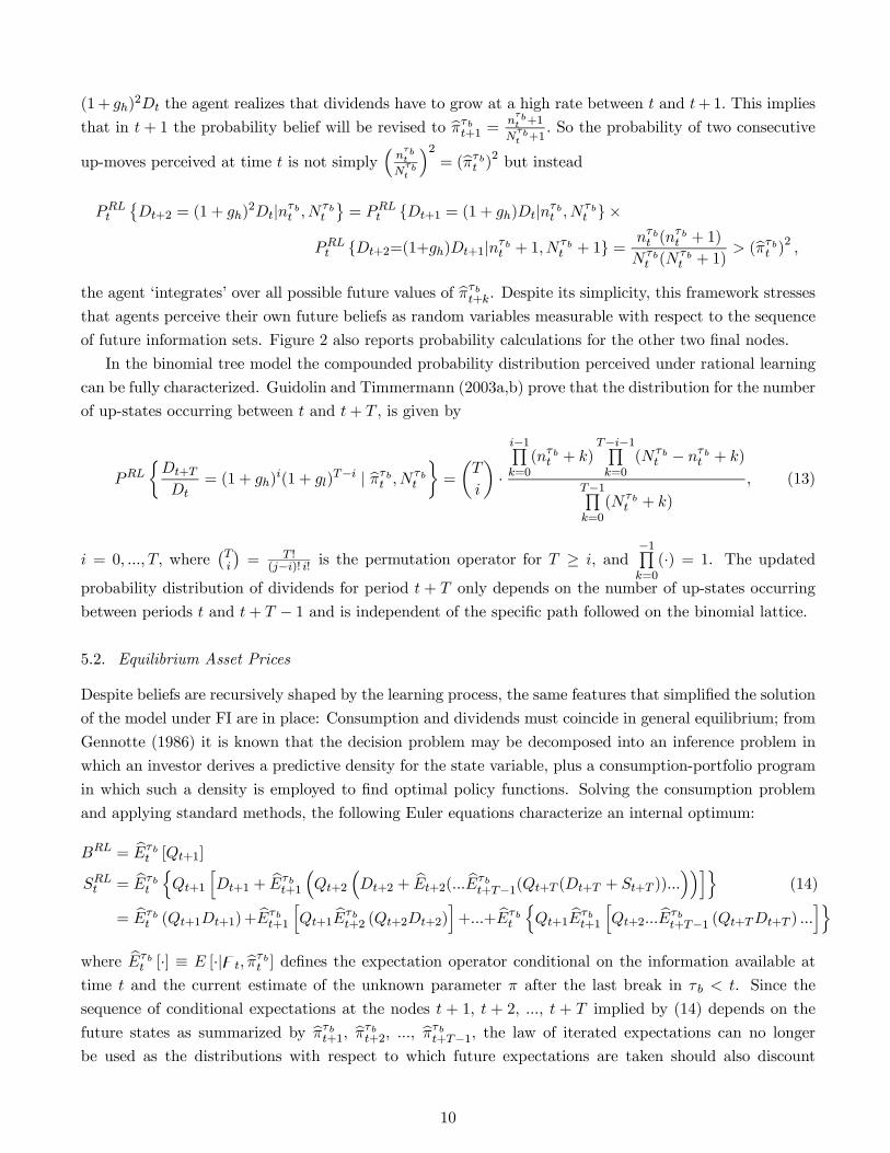
(1+ gh)2Dt the agent realizes that dividends have to grow at a high rate between t and t+1. This implies

that in t + 1 the probability belief will be revised to bπτbt+1 = nτbt +1

Nτbt +1

. So the probability of two consecutive

up-moves perceived at time t is not simply³nτbt

Nτbt

´2= (bπτbt )2 but instead

PRLt©Dt+2 = (1 + gh)

2Dt|nτbt , N τbt

ª= PRLt {Dt+1 = (1 + gh)Dt|nτbt , N τb

t } ×

PRLt {Dt+2=(1+gh)Dt+1|nτbt + 1,N τbt + 1} = nτbt (n

τbt + 1)

N τbt (N

τbt + 1)

> (bπτbt )2 ,the agent �integrates� over all possible future values of bπτbt+k. Despite its simplicity, this framework stressesthat agents perceive their own future beliefs as random variables measurable with respect to the sequence

of future information sets. Figure 2 also reports probability calculations for the other two Þnal nodes.

In the binomial tree model the compounded probability distribution perceived under rational learning

can be fully characterized. Guidolin and Timmermann (2003a,b) prove that the distribution for the number

of up-states occurring between t and t+ T , is given by

PRL½Dt+TDt

= (1 + gh)i(1 + gl)

T−i | bπτbt , N τbt

¾=

µT

i

¶·

i−1Qk=0

(nτbt + k)T−i−1Qk=0

(N τbt − nτbt + k)

T−1Qk=0

(N τbt + k)

, (13)

i = 0, ..., T, where¡Ti

¢= T !

(j−i)! i! is the permutation operator for T ≥ i, and−1Qk=0

(·) = 1. The updated

probability distribution of dividends for period t + T only depends on the number of up-states occurring

between periods t and t+ T − 1 and is independent of the speciÞc path followed on the binomial lattice.

5.2. Equilibrium Asset Prices

Despite beliefs are recursively shaped by the learning process, the same features that simpliÞed the solution

of the model under FI are in place: Consumption and dividends must coincide in general equilibrium; from

Gennotte (1986) it is known that the decision problem may be decomposed into an inference problem in

which an investor derives a predictive density for the state variable, plus a consumption-portfolio program

in which such a density is employed to Þnd optimal policy functions. Solving the consumption problem

and applying standard methods, the following Euler equations characterize an internal optimum:

BRL = bEτbt [Qt+1]SRLt = bEτbt nQt+1 hDt+1 + bEτbt+1 ³Qt+2 ³Dt+2 + bEt+2(... bEτbt+T−1(Qt+T (Dt+T + St+T ))...´´io (14)

= bEτbt (Qt+1Dt+1)+ bEτbt+1 hQt+1 bEτbt+2 (Qt+2Dt+2)i+...+ bEτbt nQt+1 bEτbt+1 hQt+2... bEτbt+T−1 (Qt+TDt+T ) ...iowhere bEτbt [·] ≡ E [·|zt, bπτbt ] deÞnes the expectation operator conditional on the information available attime t and the current estimate of the unknown parameter π after the last break in τ b < t. Since the

sequence of conditional expectations at the nodes t + 1, t + 2, ..., t + T implied by (14) depends on the

future states as summarized by bπτbt+1, bπτbt+2, ..., bπτbt+T−1, the law of iterated expectations can no longer

be used as the distributions with respect to which future expectations are taken should also discount

10

future information ßows. Once this fact is recognized, Guidolin and Timmermann (2003b) show that if a

transversality condition holds and ρ > max {g∗l , g∗h} , the stock price under rational learning, SRLt , is

SRLt = ΨRLt Dt =

∞Xi=1

βiiXj=0

(1 + g∗h)j(1 + g∗l )

i−jPRL³Djt+i|bπτbt , N τb

t

´ ·Dt (15)

where PRL³Djt+i = (1 + gh)

j(1 + gl)i−jDt|bπτbt , N τb

t

´is given by (13). The equilibrium risk-free rate is

rRLt (bπτbt ) = 1 + ρ

(1 + gl)−γ + bπτbt [(1 + gh)−γ − (1 + gl)−γ ] − 1. (16)

These results have three implications. First, the pricing kernel is no longer a constant, depending on the

cumulated knowledge on π, through nτbt and N τbt . In this sense, dividend changes between time t+ k and

t + k + 1 acquire a self-enforcing nature: news of a certain sign will cause not only a stock price change

through the linear pricing relationship SRLt = ΨRLt Dt, but also through the revision of the pricing kernel,

ΨRLt . Second, while under FI the risk-free rate was a constant, on a learning path it changes as a function

of the �new� state variables nτbt and N τbt . In particular, for γ ≤ 1 (1 + gh)

−γ − (1 + gl)−γ ≤ 0 and high

dividend growth raises the risk free rate by raising bπτbt ; the opposite when γ > 1. Third, notice that

structural breaks are reßected in equilibrium asset prices only because of their �resetting� effects on the

agents� learning clock, i.e. via nτbt and N τbt . Although structural breaks are possible at all times, their

infrequent nature makes the cost of ignoring their future occurrence small.

Guidolin and Timmermann (2003b) show that although the process of fundamentals is �smooth� (i.e.

i.i.d. and with low volatility) rational learning may generate stock prices with many realistic features,

such as serial correlation, volatility clustering, and excess volatility. However, they fail to investigate

the implications for excess stock returns and the riskless interest rate. Furthermore, it is clear that in

the absence of structural breaks agents would eventually learn the process for dividends to an arbitrary

accuracy, so that the pricing kernel ΨRLt would converge to ΨFI and all learning effects would disappear.

In other words, by assuming the observable occurrence of breaks, we rule out the possibility of complete

information, see Timmermann (2001, p. 302).

6. Implications for the Equity Premium

6.1. Full Information Rational Expectations

In the FI case, the mapping simpliÞes to a relation between preferences [ρ γ]0 and equilibrium asset returns.It is straightforward to derive the expression for the equity premium:

Ehrp,FIt

i= (1 + ρ)

½1 + gl + πt(gh − gl)1 + g∗l + πt(g

∗h − g∗l )

− 1

(1 + gl)−γ + πt [(1 + gh)−γ − (1 + gl)−γ ]¾. (17)

Since dividends are i.i.d., there is no difference between the time t conditional and unconditional equity

premium. Moreover, besides the parameters {gh, gl,πt} , (17) depends on [ρ γ]0 only. To stress this

dependency, we write E[rp,FIt (ρ, γ)] and rf,FI(ρ, γ). It is then natural to ask what are the limits of

Ehrp,FIt

ias [ρ γ]0 vary, i.e. does a preference structure exist such that the stylized facts can be matched?

From Section 4, it makes no sense to ask what happens to asset returns when γ → ∞ or γ → 0

irrespective of ρ, i.e. to consider independent limits. Since we have assumed that gl < 0, for given ρ when

11

γ → ∞ we incur in a violation of (8). Therefore we restrict ourselves to a range of relative risk aversion

that ensures Þnite stock prices, [0, γ̄), where γ̄ > 1 is deÞned as the CRRA such that:

1 + ρ = πt£(1 + gh)

1−γ̄¤+ (1− πt) £(1 + gl)1−γ̄¤ (18)

Therefore we will take limits as γ % γ̄ (from the left). As for the limit of expected asset returns as γ & 0

(from the right), since gh > 0 it is possible to Þnd a γ< 1 such that:

1 + ρ = πt£(1 + gh)

1−γ¤+ (1− πt) £(1 + gl)1−γ¤ (19)

and (8) fails to hold for γ <γ. We write γ &γ, under the understanding that γ may be zero.The following result characterizes the basic properties of asset returns in this artiÞcial economy. To

simplify its statement, deÞne γf and γe as the coefficients of relative risk aversion such that:

−πt(1 + gh)−γf ln(1 + gh)− (1− πt)(1 + gl)−γf ln(1 + gl) = 0 (20)

−πt(1 + gh)1−γe ln(1 + gh)− (1− πt)(1 + gl)1−γe ln(1 + gl) = 0, (21)

if solutions to the equations exist.

Proposition 1. Under full-information rational expectations:

(a) Given ρ ≥ 0, for γ < γf , rf,FI(ρ, γ) is an increasing function of γ, while for γ > γf , rf,FI(ρ, γ)decreases in γ so that rf,FI(ρ, γ) < 0 is possible. If γf is not deÞned, then rf,FI(ρ, γ) is always monotone

decreasing in γ.

(b) Independently of other conditions, E[rp,FIt (ρ, γ)] ≥ 0, E[rp,FIt (ρ, 0)] = 0. γf ≤ γe so that, given

ρ ≥ 0, there exists a γmax (γf ≤ γmax ≤ γ̄) such that for γ below γmax E[rp,FIt (ρ, γ)] is an increasing

function of γ, while for γ > γmax, E[rp,FIt (ρ, γ)] decreases in γ.

Proof: See Appendix.

The proposition offers direct implications for the possibility to produce under full information a risk-

free rate and an equity premium consistent with the evidence. The naive notion that a high coefficient of

relative risk aversion γ can offer a way to resolve the puzzles does not apply to our model. From (b), we

can only hope that γ̄ is high enough to span an interval that includes a γmax such that a risk premium as

high as in the data obtains. Section 7 examines whether in a standard calibration exercise a model with

FI does stand any chance to match observed features of asset returns series.

6.2. Rational Learning

Under RL preferences impact on equilibrium prices in a way that depends on the state of beliefs. From

(15), SRLt = ΨRL(nτbt ,Nτbt ; ρ, γ)Dt. Therefore � assuming the absence of a structural break between t and

t+ 1 � the excess stock return over the interval [t, t+ 1] is:

rp,RLt+1 (nτbt , N

τbt , n

τbt+1; ρ, γ)=

(1 + gt+1)

ΨRL(nτbt , Nτbt ; ρ, γ)

+ΨRL(nτbt+1, N

τbt +1; ρ, γ)

ΨRL(nτbt , Nτbt ; ρ, γ)

(1+gt+1)− 1− rf,RLt (nτbt , Nτbt ; ρ, γ).

(22)

On a learning path, realized excess equity returns depend on both agent�s initial beliefs (nτbt , Nτbt ) as well

as on their change between t and t+ 1 (through the ratio ΨRL(nτbt+1, Nτbt + 1)/ΨRL(nτbt , N

τbt )).

12

A different concept is the equity premium expected at time t, conditional on the information on the

process for dividends then available (nτbt , Nτbt ):

�Eτbt

hrpRL,t+1 (ρ, γ)

i=�Eτbt [(1 + gt+1)]

ΨRLt+�Eτbt [(1 + gt+1)Ψ

RLt+1]

ΨRLt− 1 + ρ

�Eτbt [(1 + gt+1)−γ]. (23)

Notice that (23) represents a subjective notion of the equity premium as a subjective expectation operator�Eτbt [·] that depends on the agents� information set (nτbt , N τb

t ) is employed. Importantly,

Ehrp,RLt+1 (ρ, γ)

i6= E

n�Eτbt

hrp,RLt+1 (ρ, γ)

io,

i.e. the objective unconditional equity premium (left-hand side) on a rational learning path differs from the

objectively expected subjective equity premium (right-hand side). This difference raises an important issue.

Traditionally, the literature has discussed the circumstances under which a model generates a stationary

distribution for excess returns matching sample moments. In particular, the equity premium E[rpt+1(ρ, γ)]

is identiÞed with a long-run sample mean of excess equity returns. While E[rp,RLt+1 (ρ, γ)] can be quantiÞed

by simulating prices in (22) and (16) and taking averages over simulation trials, this quantity is in general

different from the estimate of En�Eτbt

hrp,RLt+1 (ρ, γ)

iothat can be similarly obtained by simulation. Although

the average (expected) subjective equity premium may be possibly interesting in itself (see Abel (2002) and

Section 8.4), it is clear that the only quantity that can be directly compared to the data is E[rp,RLt+1 (ρ, γ)].

While the current section reports results for the objective conditional expectation of the equity premium

under RL, Section 7 uses simulations from a calibrated version of our model to produce results on the

objective unconditional equity premium to be compared with the evidence from Section 2. A Lemma in

Guidolin and Timmermann (2003b) shows that ΨRLt is an nondecreasing and convex function of bπτbt when

γ ≤ 1, and a decreasing and convex function of bπτbt when γ > 1. Based on this result, it is possible to prove:

Proposition 2. γ < 1 and pessimistic beliefs ( bπτbt < πt) imply

rf,RLt (ρ, γ) < rf,FI(ρ, γ)

Et[rp,RLt+1 (ρ, γ)] > E[rp,RLt+1 (ρ, γ)].

Proof: See Appendix.

We are able to isolate a combination of risk-aversion and beliefs � low risk aversion and pessimism �

for which the conditional risk premium is higher under RL than the (unconditional) risk premium under

FI. In principle, the incorporation of learning effects points in the direction of higher equity premia for

plausible preferences, provided the economy is characterized �on average� by some degree of pessimism.

Moreover, under the same assumptions, rf,RLt (ρ, γ|nτbt , N τbt ) ≤ rf,RL(ρ, γ) should make the occurrence of a

risk-free rate puzzle unlikely.

Contrary to the FI case, under RL it is extremely difficult to characterize the behavior of equilibrium

expected returns and of the equity premium as a function of preference parameters only. In fact, no

analog to Proposition 1 can be proven because ρ and γ have effects on asset returns that depend on

the state of beliefs. For instance, if there is pessimism and relative risk aversion is progressively lowered

towards zero, the conditional premium can increase, a somewhat counter-intuitive result. The intuition is

that as an economy becomes risk-neutral, the intertemporal elasticity of substitution (1/γ) diverges and

rf,RLt (ρ, γ) % ρ as the demand for bonds increases for consumption smoothing. As for stock returns, the

13

RL pricing kernel increases in bπτbt faster and faster as γ & 0. However, as we approach risk-neutrality,

the growing ΨRLt reduces the contribution of dividend growth to stock returns. The Þrst effect reßects the

fact that under near-risk-neutrality the agents will revise the kernel ΨRLt (bπτbt ) more heavily as �πt % π,

i.e. starting from pessimistic beliefs learning gives a stronger contribution to high realized excess returns

through the elimination of the undervaluation. The second effect reßects the pure decline of dividend yields

as we approach risk-neutrality. Although which of the two effects dominates is a function of gh, gl, ρ, andbπτbt , if γ is close to zero the former effect will prevail and the conditional premium increases as γ & 0.

Since also the risk-free rate decreases, the equity premium increases.

7. Simulations

7.1. Model Calibration

We set a yearly ρ = 0.02, which implies an annual discount factor β ' 0.98, a common value in the literature.In the tradition of MP, we experiment with alternative levels of relative risk aversion. Suppose that real

consumption growth changes at quarterly frequency. So its annual rate of growth follows a transformation

of Bi(4,π) process. We condition our exercise on the fact that US investors observed the two structural

breaks in real consumption uncovered in Section 2.1. Therefore we perform a double calibration exercise:

the Þrst with reference to the period 1938-1981, the second with reference to the period 1982-1999.

With reference to the period 1938-1981, we calibrate the quarterly growth process by taking gh = +1.5%,

gl = −1.25%, and π = 0.645. These parameters guarantee an annual mean growth of 2%, an annual

volatility of 2.6%, while the annual growth rate is positive 87% of the time. On a learning path initial

beliefs n0 and N0 concur to determine the equity premium. During the depression period 1930-1937,

the average real consumption growth had been -0.5% and growth had been negative half of the time.

Undoubtedly, beliefs had to be pessimistic. In particular, the �π19380 that makes the assumed quarterly

process for dividends compatible with real consumption declining 50% of the time at an annual level is:

4Xi=0

I{(1.011)i(0.995)4−i<0}

µ4

i

¶¡bπ19380

¢i ¡1− bπ19380

¢4−i=¡1− bπ19380

¢4+ 4bπ19380

¡1− bπ19380

¢3 ∼= 0.50. (24)

bπ19380 = 0.35 approximately satisÞes (24) and implies a slightly negative expected real growth of consump-

tion (-0.3%), a pessimistic albeit not extreme belief. bπ19380 must be assigned some weight, a measure of

its strength against subsequent information. Although the experience of the Great Depression is likely to

have left a big mark on collective beliefs, we limit its precision to 32, the number of quarters in the cycle

1930-1937 (NBER dating). Therefore �n19380 = 11 and �N19380 = 32 so that �n19380 / �N1938

0 ' 0.35. In our view,calibrating a pessimistic belief for the post-Depression era is merely a way to give content to the claim that

�(...) the experience of the Great Depression (...) [had] a signiÞcant inßuence on the behaviour of those

who experienced it directly or indirectly (...)� (Danthine and Donaldson (1999, p. 608)).

The second calibration exercise concerns the period following the structural break determined by the

oil shocks of the 1970s. We calibrate the quarterly process of consumption growth by taking gh = +1.5%,

gl = −1.25%, and π = 0.63. These parameters imply an annual mean of 1.9% and annual volatility of

2%. During the cycle 1974-1981, average real consumption growth has been lower than in the 1960s and

recollection of the pessimistic evaluations of the growth slowdown of those years makes a parameterization

of the initial beliefs reßecting some degree of pessimism plausible. It is easy to verify that bπ19820 = 0.5

14

produces an annual mean growth rate of 0.4%, a volatility of 2.8%, and positive rates of annual growth

69% of the time. These features closely match the process of real fundamentals during the late 1970s. We

also set �N19820 = 8 (the number of quarters in the cycle 1980-1981) and therefore �n19820 = 4.

7.2. The Equity Premium under Full Information

In the full-information case, it is straightforward to calculate γ= 0 and γ̄ ' 58.8: outside this interval

the FI equilibrium fails to exist. Figure 3 depicts the equity premium and the risk-free rate under FI

when γ changes and no breaks are imposed. Notice that under FI no simulations are required since the

expectations involved by (17) can be directly evaluated. The equity premium puzzle admits no solution: an

average risk-free rate below 1% per year can be attained only using a constant relative risk aversion above

57. Incidentally, the available window is also very narrow as γ̄ ' 58.8 and for γ > 58 the real risk-free

rate becomes negative, which is counterfactual. However, even for risk aversion coefficients as high as 58,

the ex-ante expected risk premium is at most 3.8%. Assuming that the consumption growth process is

adequately described by a binomial lattice, it is impossible to Þnd a level of risk aversion such that ex-post

realized excess returns in the order of 7% are generated.

7.3. The Equity Premium under Rational Learning

For alternative levels of γ, we simulate Z = 10, 000 independent, quarterly time paths for real dividends

and equilibrium asset prices when the agent is on a rational learning path and breaks occur in 1938 and

1982. After each break, initial beliefs are calibrated to plausible values as of January 1938 (�n19380 = 11,�N19380 = 32) and January 1982 (�n19820 = 4, �N1982

0 = 8). Fundamentals are drawn according to the

parameters discussed in Section 7.1. The time paths have a length equal to the post-depression period

1938-1999, 248 quarters. Since the statistical properties we match refer to annual series, after simulating

248-quarter long series for dividends and prices, we aggregate them to obtain 62-year long annual series.

One issue that arises when assessing asset pricing properties on a learning path by simulation is the

existence of the equilibrium along the entire simulated path. Indeed the market belief bπτbt changes as new

realizations of the growth process come along. From Section 5 we know that given ρ > 0 and bπτbt , γ 6= 1could be chosen either too large or too small in order for the equilibrium to exist at time t. In particular,

when beliefs are strongly pessimistic (bπτbt << π), γ >> 1 might be excessive to support the equilibrium. It

is also possible that strongly optimistic beliefs (bπτbt >> π) might disrupt the RL equilibrium when γ << 1.

The occurrence of any violation at any point of a simulated path t = 1, ..., T invalidates the ability of the

path itself to represent an equilibrium outcome from an artiÞcial RL economy. We handle the issue in a

pragmatic way. First, we limit the simulations to an interval for the coefficient of relative risk aversion such

that divergence of (15) is unlikely, γ ∈ [0.3, 2]. This is also the interval including values of the coefficientof relative risk aversion that are commonly thought of as plausible. Second, we check convergence of (15)

monitoring the progressive shrinking of the contribution to SRLt of successive terms in (15).

Figure 4 plots the unconditional premium and the risk-free rate when agents are on a rational learning

path and perceive two breaks vs. the FI case. In practice, we report the quantity

1

Z

ZXj=1

1

T

TXt=1

rp,RLt,j (nτbt−1,j , Nτbt−1, n

τbt,j)

15

rp,RLt,j (nτbt−1,j , Nτbt−1, n

τbt,j) ≡

(1 + gt,j)

ΨRL(nτbt−1,j , Nτbt−1)

+ΨRL(nτbt,j , N

τbt−1 + 1)

ΨRL(nτbt−1,j , Nτbt−1)

(1 + gt,j)− 1− rf,RLt,j (nτbt−1,j , Nτbt−1),

where j = 1, 2, ..., Z indexes simulation paths, and nτbt,j evolves randomly on each path. Other unconditional

moments are deÞned similarly. 90% conÞdence bands are also plotted. As for the FI values, they are

obtained by simulation as well since the occurrence of breaks slightly changes results relative to Figure 3.

As shown by Proposition 2, γ < 1 combined with pessimism pushes the RL premium higher than under FI.

In particular, the RL equity premium is decreasing in γ < 1, so a moderate curvature of the utility function

is consistent with generating high excess returns. For instance, for γ = 0.3 the equity premium over the

62 years covered by the exercise is 5%, a remarkable result in the premium literature. A 90% conÞdence

interval generated from the distribution of the simulated equity premia under RL is wide ([3, 7.1]), including

premia close to the 7.6% target reported in Section 2 (and represented by a solid bar in the plots). 51%

of the simulations generated equity premia in excess of 5%, and many (about 24%) were above 7%. For

γs above 1.3 the equity premium becomes negative, an indication that downward revisions of ΨRLt as bπτbtmoves (on average) towards π reduce realized excess returns. The annual rate of return on short-term

bonds is always above 2 percent, above the 1 percent observed over the period 1938-1999. In fact, under

both RL and FI, it takes a downward drifting endowment process in order to produce equilibrium values

of the risk-free rate below 2%. However, Figure 4 also shows that � relying on a low γ � a learning-based

explanation does not incur in the risk-free rate puzzle.

A point often insisted upon (Cecchetti et al. (2001)) is that proposed resolutions to the equity premium

puzzle have been moderately successful at reproducing Þrst moments but that difficulties remain when it

comes to match higher-order moments, in particular variances. Under FI and regardless of the presence

of breaks, equity returns inherit the stochastic properties of the endowment process. Since the growth in

fundamentals is assumed to be i.i.d. and is calibrated to match the smoothness of the US economy, it

implies not only a non-volatile, i.i.d. process for excess returns, but also a constant interest rate. Hence

the FI model stands no chance to reproduce the excess volatility of stock returns vs. consumption growth.

On the opposite, under the RL model the volatility of real stock returns and excess equity returns can be

easily matched (at roughly 18%). Moreover, realistic variability in the equilibrium interest rate appears.

7.4. Matching Other Properties of Asset Returns

A point often insisted upon (Cecchetti et al. (2001)) is that proposed resolutions to the equity premium

puzzle have been moderately successful at reproducing levels of the risk-free rate and of the risk-premium,

although difficulties remain when it comes to match higher-order moments, for instance variances. Since

Table I has also reported other descriptive statistics concerning real stock returns, excess returns, and short-

term yields, we engage in the same type of evaluation for asset returns simulated from the model. Given

preferences [ρ γ]0, for each simulation trial we calculate descriptive statistics χj(ρ, γ|�n0, �N0) (j = 1, ...,

Z) and report averages χ̄(ρ, γ|�n0, �N0) ≡ Z−1PZj=1 χj(ρ, γ|�n0, �N0). Figures 5-7 plot the following (average)

statistics as a function of relative risk aversion: excess returns standard deviation, the percentage of

simulations for which the null hypothesis of zero serial correlation is rejected at a nominal size of 5% (using

the Ljung-Box statistic of order 8), the percentage simulations for which the null of no serial correlation

in squared asset returns is rejected at 5% (using the LB(8) statistic, interpreted as a test of volatility

16

clustering), and the correlation between interest rates and excess returns.

Under FI and regardless of the presence of breaks, the model is clearly incapable of capturing some

stylized facts: Equity returns simply pick up the stochastic properties of the assumed process of endowment

growth. Since the growth in fundamentals is assumed to be i.i.d. and is calibrated to match the smoothness

characterizing the US economy, it implies not only a non-volatile, i.i.d. process for excess returns, but also

a constant interest rate. Hence the FI model stands no chance to pick up interesting stylized facts, such

as excess volatility of stock returns vs. consumption growth, and the rich statistical properties of the real

risk-free rate.10 As far as RL is concerned, Figure 5 shows that for a small γ < 1 the volatility of real

stock returns and excess equity returns can be easily matched. However this conclusion does not fully

apply to the risk-free rate: although RL produces time variation, it is insufficient. On the other hand, it

is remarkable that learning can generate sufficient variation in real stock prices at the same time matching

the volatility of fundamentals and not producing excessive variation in riskless interest rates, a result that

has proven elusive in previous research (see Cecchetti et al. (1990)).

Figure 6 focuses on serial correlation and volatility clustering. Table I shows that while annual real

and excess returns on equities display no sign of serial correlation or ARCH, the opposite holds for the

risk-free rate that has long memory. Under RL, simulated real and excess stock returns display some mild

structure in the Þrst two moments when γ is small, as evidenced by a percentage of simulations between 30

and 50 that show a signiÞcant Ljung-Box statistic at 5%. As γ increases above one, these Þgures rapidly

increase above 90%, sign of strong and counterfactual correlation and volatility clustering. In the case of

the risk-free rate, independently of γ almost 100 percent of the simulations display signiÞcant correlation

both in returns and in squared returns. Finally, Figure 7 plots the average simulated correlation coefficient

between excess returns and the real-risk free rate. In this case, the stylized fact to be matched is a small,

negative correlation (-0.05). It is clear that FI has an advantage, since (apart from breaks) the FI risk-free

rate is constant and uncorrelated with any other random variable. On the other hand, the graph shows

that for small values of γ the average simulated correlation is low (-0.15), as required. We take Figure 7

as evidence favorable to a learning based explanation of US asset returns in the XXth century.

7.5. A Path Calibration

As a more stringent test of the model�s predictive ability, we perform a path-calibration: since realized

consumption growth rates are observed for every year of the period 1938-1999, we Þt the binomial lattice

to the data and let our representative agent learn π by using the sign of realized changes in consumption

to infer whether gt equals either gh > 0 or gl < 0. This calibration strategy is similar to Brennan and

Xia (2001). Figure 8 shows the dynamics of bπτbt implied by US consumption data at annual frequency.

The effects of the Great Depression are evident, as bπτbt starts declining in 1929. The big jump at the

end of the 1930s is also caused by the assumption that agents perceived a break in 1938 and re-started

their estimation from pessimistic beliefs (�n19380 = 2 �N19380 = 8, annualizing quarterly values). Despite a

slowdown at the end of the 1940s, the three decades following 1938 are marked by rapid upward revisions

of bπτbt . By the early 1970s, �π ' 0.75 implying a perceived high mean growth rate and moderate volatility.The oil shocks end this booming period and induce an early 1980s break, characterized by mild pessimism

(�n19820 = 1 �N19820 = 2 consistently with previous choices).

10The FI statistics simply consist of straight lines that do not depend on the relative risk aversion coefficient.

17

The right panel shows equilibrium stock prices obtained assuming ρ = 0.02 and γ = 0.3. For most of

the sample period, FI prices stay above the RL ones. When at the end of the 1990s the perception of π

eventually catches up with values consistent with the statistical properties of US consumption data, RL

and FI prices converge. The (unreported) simulated riskless rate shows that as pessimism is imposed, the

RL rate remains below the FI rate, barely exceeding a plausible level of 3% on average. We extend the

exercise and calculate equity premia and excess return volatility for all levels of γ in [0.3, 2].11 Results are

qualitatively similar to those in Section 7.3 and are quantitatively interesting for low risk aversion. When

γ = 0.3 we Þnd an equity premium of 3.3% and an average riskless interest rate of 3.2% for the period

1938-1999. The corresponding values under FI are 0.7% and 3.6%. As obtained before, the equity premium

is monotone decreasing in γ (over the [0.3, 2] interval). Although an equity premium of 3.3% does not

entirely solve MP�s puzzle, the ability of the model to explain roughly half of MP�s puzzle is encouraging.

7.6. Dynamic Properties

A further set of restrictions implied by RL can be tested: on one hand, since learning is stronger in

the aftermath of structural breaks, the data should display deviations from the unconditional (full-sample)

statistical properties− such as higher than average equity premia and volatility − over the periods followingbreaks; on the other hand, since we have calibrated initial beliefs to reßect some pessimism in the aftermath

of breaks, our simulations ought to generate these stronger deviations from FI.

We study these implications in two ways. First, Figure 9 shows that there is evidence in the data

of higher equity premia and volatility in the aftermath of breaks (the solid vertical lines in the plots).

The top graph plots 10- and 15-year forward rolling window equity premia calculated by collecting partial

samples at each date between 1930 and 1990 and averaging excess equity returns over these intervals.12

The bottom graph does the same with reference to sample standard deviations. The solid horizontal lines

provide unconditional benchmarks, 7.1% and 19.5% for the equity premium and volatility. Clearly, all

potential breaking dates are followed by above average conditional equity premia, both on 10- and on

15-year sub-samples. For instance, using 15-year windows 1938 is followed by a 11% premium, 1982 by a

10.1% premium. Results for volatility are instead mixed: while the 1930s break is certainly followed by

above-normal volatility, this does not happen for other breaks, notably for the one in the early 1980s. In

this sense, our model seems to propose a plausible explanation for the high equity premium phenomenon

but shows some difficulty at generating the correct dynamic volatility patterns.

Second, we use the path calibration of Section 7.5 to measure a few properties of excess returns over

periods that follow the two structural breaks; we use also in this case two identical 15-year long sub-samples,

i.e. 1938-1952 and 1982-1996. For ease of exposition we report a single arithmetic average over the two

periods. We Þnd indeed evidence of stronger deviations from FI in the aftermath of breaks: for γ = 0.3

the equity premium is 7.1% and the standard deviation of excess returns is 22.7%.

11We set the parameters as: gh = +3.1% and gl = −0.7%; although the choice of π is irrelevant for RL prices, it mattersfor FI results and we pick π = 0.795. For the period 1982-1999 we set identical gh and gl, and π = 0.78.12For instance, we consider the 1930-1939 (10-year window) and 1930-1944 (15-year window) samples, calculate mean excess

equity returms, and report the results in correspondence to 1930.

18

8. Discussion

8.1. The Role of Initial Beliefs

We perform robustness checks on initial beliefs: Would the results be stronger if beliefs in the aftermath

of the Great Depression had been even more pessimistic than assumed? To provide some answers to

these questions, we set two alternative values of γ (0.2 and 2) and proceed to calculate E[rp,RLt (ρ, γ)] and

E[rf,RLt (ρ, γ)] with �N0 = 32 as in Section 7.3 but with �n0 that changes between �n0 = 9 (�π0 = 0.28) and

�n0 = 22 (�π0 = 0.69) in steps of two (i.e. �n0=11, 13, etc.) whenever possible.13 Figure 10 shows that when

γ < 1, pessimistic initial beliefs are not required. Even when �π0 = π, γ = 0.2 gives an equity premium of 2

percent, with a 90% conÞdence band wide enough to include premia of 3.5 percent. Moreover, should we

Þnd a reason to specify beliefs more pessimistic than �π19380 = 0.35, we would provide complete solution to

the equity premium puzzle. When γ = 0.2 and �π0 = 0.28, the equity premium is 6 percent and the 90%

conÞdence band spans the interval [3.2, 8]. Finally, for γ = 2 even optimism does not help. For instance

�π0 = 0.59 produces a negative premium. Our intuition is that optimism raises the risk-free rate faster than

expected stock returns, thus reducing the premium.

8.2. Integrating out Initial Beliefs

We study whether rational learning can contribute to our understanding of the equity premium and risk-

free rate puzzles when no restrictions on initial beliefs are imposed and time τ b beliefs are integrated out.

Suppose we take an agnostic view on beliefs at the beginning of 1938, admitting pessimism and optimism in

equal degrees. Assume that given �N19380 = 32, the initial belief �π19380 could have been with equal probability

any value in the interval [0.445, 0.845], symmetric around the unknown π = 0.645, i.e. �π19380 is assumed

to have a uniform prior density.14 We evaluate asset returns on a rational learning path by simulating

time series for the real endowment and equilibrium prices 50,000 times, when in correspondence to each

simulation the initial belief is drawn afresh from a uniform prior in independent fashion. Thus while Section

7.3 has focused on Ehrp,RLt (ρ, γ|�π0)

itaking �π0 as given, we now calculate:

Ehrp,RLt (ρ, γ)

i=

Z 0.845

0.445Ehrp,RLt (ρ, γ|�π0)

id�π0, (25)

where �π0 = bn0/ �N0.15 Again, we set ρ = 0.02 and vary γ over the interval [0.3, 2].Figure 11 gives an encouraging picture. Even imposing no assumptions on initial beliefs, a model

incorporating learning effects gives an appreciable contribution to explain the two asset pricing puzzles,

provided γ is less than one. For a low γ, the equity premium exceeds 3% and the 90% conÞdence band is

[1.7, 5.1]. The risk-free rate is 3.4%. Interestingly, these unconditional expectations are obtained without

imposing absurd degrees of curvature on the utility function. This result is made possible by the combina-

tion of two factors: Firstly, the equilibrium risk-free rate is low when γ is low independently of the state of

beliefs; Secondly, when γ < 1 the price-dividend ratio is increasing and convex in �πt, implying that upward

13The inÞnite sum deÞning the RL pricing kernel may not converge. In fact with very low γs (such as 0.2) the equilibrium

is unlikely to exist for high �n0s, i.e. optimistic beliefs.14The length of this interval is arbitrary. However all other beliefs seem to be extreme and implausible. For instance,

�π0 = 0.845 implies a yearly mean growth rate of 4.4%, which is rather exceptional for a developed country.15We apply a similar randomization to initial beliefs as of 1982. Given �N1982

0 = 8, the initial belief �π0 is drawn with equal

probability on the interval [0.43, 0.83], symmetric around the unknown π = 0.63.

19

revisions of beliefs typical of pessimistic economies will have a stronger (positive) effects on equity returns

than the downward revisions that dominate in optimistic economies.

8.3. Number and Dating of the Breaks

Up to this point we have identiÞed 1938 and 1982 as the dates in which breaks in the endowment process

occurred. Both breaks occur during protracted and deep recession phases (according to official NBER

dating): the Þrst break between 1937 and 1938 (cycle 1933-1937), the second between 1980 and 1981 (cycle

1981-1982). However, the two dates used in our calibration were selected as the year(s) containing the

end quarter of the recession periods during which the break was perceived. One might wonder about what

happens to the number and nature of the breaks in the case in which the Þrst break is associated with (say)

1932 instead of 1938. Conditional on a 1932 break, we perform a statistical analysis similar to Section 2.1

(still taking the minimum no-break period to be ι = 20 years) and uncover some evidence of a break in the

drift parameter µ in the early 1950s, particularly in 1954. Interestingly, the 1954 break is another �negative�

break in the sense that it can be once more characterized by a downward revision of growth expectations

on the US economy: while during the New Deal and during WWII fundamentals grew at high rates (e.g.

the implied unconditional growth rate is 5.4% over the interval 1933-1946), after the end of WWII the US

economy experienced a structural slowdown that agents might have perceived as a break. For instance,

using data for the period 1933-1954, the implied unconditional growth rate would have been 2.9% only,

indication of a remarkable slowdown in 1947-1954. When we condition on a break in 1954, there is once

more evidence of a third break in correspondence of the oil shocks, although some uncertainty now exists

on the dating: while the drift parameter implies a break as early as 1974, the AR(1) coefficient gives weak

indication for 1975 and strongly signals a break as late as 1982, after the second shock. In any event, the

entire period 1974-1982 matches a famous episode of slowdown of the US economy (see Maddison (1987)).

What matters for our purposes are the asset pricing effects of a third break. Notice that the early

1950s represent a period in which the US economy cools off after the rapid growth caused by the war

effort. Therefore, if perceived by the agents, the 1954 break is likely to have been accompanied by relatively

pessimistic beliefs: 1948, 1949, and 1954 were all recession years with nonpositive real consumption growth;

while in 1933-1946 the average annual consumption growth had been 3%, in the interval 1947-1954 it

declines to only 0.4%. Similarly to Section 7.1, we set �π19540 = 0.5 and �N19540 = 32 (hence �n19540 = 16),

corresponding to the sequence of short recession periods characterizing the interval 1947-1954. We then

repeat the simulation experiments.16 For γ = 0.3 the equity premium over the 68 years covered by the

exercise is 4.7% while the riskless interest rate is 3.2%. The annualized volatility of excess equity returns

is 18.8%. Roughly 60% of the simulations exceed 5%. Hence our results on the possibility of generating

equity premia in the order of 5% and interest rates below 3% with low risk aversion do not depend on

either the exact number and location of the breaks or on the details of the calibration of initial beliefs.

8.4. Doubt, Pessimism and Rational Crash Fears

Abel (2002) shows that pessimism and doubt on the distribution of future consumption growth rates may

provide a solution to the puzzles. It is therefore interesting to link our Þndings to Abel�s and show that

rational learning endogenously generates pessimism and doubt. Figure 12 shows the evolution over the

16We set gh = +1.5%, gl = −1.25%, π = 0.635 (1932-1954), π = 0.665 (1955-1981), and π = 0.63 (1982-1999).

20

interval 1938-1999 of the subjectively perceived distribution of the 5- and 50-years ahead real consumption

growth rate when the representative agent is under RL, {PRL(Cjt+i/Ct|bπτbt , N τbt )}ij=0, i = 20, 200. These

distributions are obtained as averages of distributions calculated according to (13) along the 10,000 sample

paths of Section 7.3. The same calibration is used. Right plots show a few selected subjective distributions

compared to the FI (approximately) normal benchmark. The support of the distributions has been re-scaled

to display annualized growth rates.

Abel (2002) deÞnes pessimism as the case in which the RL predictive distribution is Þrst-order stochas-

tically dominated by the FI one. Pessimism reduces the equilibrium risk-free rate. Figure 12 shows that

under rational learning pessimism clearly dominates. Although not reported, the implied cumulative dis-

tribution functions display the desired pattern of stochastic dominance. Of course, the effect is stronger in

the 1940s and again in the 1980s, but it seems that a rational agent might have underestimated the overall

location of the distribution of future growth rates for long periods. The effects on the risk-free rate are

qualitatively similar, as shown by Proposition 4, provided γ < 1. Abel (2002) strengthens his deÞnition

to uniform pessimism, when the subjective distribution lies entirely to the left of the objective one, with

no contact points. Uniform pessimism is sufficient to inßate the equity premium. Figure 12 stresses that

uniform pessimism obtains at many dates in our calibration. The effect on the equity premium is similar

and obtains through the convexity of the RL pricing kernel for γ < 1: since upward revision of beliefs

increase prices more than downward revisions, in a pessimistic economy the former are more likely than

the latter and this impresses a substantial upward drift to equilibrium stock prices.

Abel deÞnes doubt as the case in which the RL predictive distribution is a mean-preserving spread

of the FI one. He shows that since the pricing kernel is convex, doubt will decrease the risk-free rate

and increase the equity premium. Figure 12 provides evidence that, independently of their location,

{PRL(Cjt+i/Ct|bπτbt , N τbt )}ij=0 describes a leptokurtic distribution with much thicker tails than the FI bench-

mark. Once more, in our framework doubt is reßected in a higher equity premium because for γ < 1 the

pricing kernel ΨRLt is a convex function of bπt. Therefore when rational learning is supplemented with his-torical evidence on the US economy, pessimism and doubt do emerge in endogenous fashion, increasing the

risk premium on equities for moderate degrees of curvature of the utility function.

9. Conclusion

This paper shows that there exists an alternative way in which extreme events such as the Great Depression

or the oil shocks can generate high equity premia. While previous literature has focused on the induced,

permanent biases in the stationary beliefs of investors in an ad hoc fashion, we show that if agents are

on a recursive learning path, tail events may produce long-lasting effects on equilibrium prices. For our

calibration of beliefs in the aftermath of the depression and the oil crises, we obtain that equity premia in

the order of 4 to 5 percent are compatible with complete markets, the absence of friction, and power utility

with a reasonable degree of curvature. These Þgures come close to the original size of the equity premium

pointed out by Mehra and Prescott and explain more than 60 percent of the average excess returns on

stocks for the post-depression period 1938-1999. The resulting conÞdence bands for the equity premium

expected as of 1938 are wide, including premia in the order of 8 percent. The equilibrium risk-free rate is

in the order of a realistic 2 percent. The model also matches the observed variance of the risk premium and

of real stock returns over the period 1938-1999, thus showing that the high volatility of real stock returns

21

in excess of real consumption growth is no puzzle.

Section 8.2 has made our case stronger by showing that the results are only slightly weakened when no

restrictions are imposed on initial beliefs and the artiÞcial economy is simulated starting from beliefs drawn

from an ignorance prior. In this case we generate equity premia in the order of 3 percent, with conÞdence

bands wide enough to include 7 percent premia. These Þndings require the use of low risk aversion levels,

so that we avoid falling in the criticized set of explanations that rely on high risk aversion.

References

[1] Abel, A., 2002, �An Exploration of the Effects of Pessimism and Doubt on Asset Returns�, Journal

of Economic Dynamics and Control, 26, 1075-1092.

[2] Aiyagari, R., and M. Gertler, 1991, �Asset Returns with Transactions Costs and Uninsured Individual

Risk�, Journal of Monetary Economics, 27, 311-331.

[3] Barsky, R., and B., De Long, 1993, �Why Does the Stock Market Fluctuate?�, Quarterly Journal of

Economics, 108, 291-311.

[4] Brennan, M., and Y., Xia, 2001, �Stock Price Volatility and Equity Premium�, Journal of Monetary

Economics, 47, 249-283.

[5] Bullard, J., and J., Duffy, 2001, �Learning and Excess Volatility�, Macroeconomic Dynamics, 5, 272-

302.

[6] Campbell, J., and J., Cochrane, 1999, �By Force of Habit: A Consumption-Based Explanation of

Aggregate Stock Market Behavior�, Journal of Political Economy, 107, 205-251.

[7] Cecchetti, S., P. Lam, and N., Mark, 1990, �Mean Reversion in Equilibrium Asset Prices�, American

Economic Review, 80, 211-242.

[8] Cecchetti, S., P. Lam, and N., Mark, 2000, �Asset Pricing with Distorted Beliefs: Are Equity Returns

Too Good To Be True?�, American Economic Review, 90, 787-805.

[9] Chu, C., M., Stinchcombe, and H., White, 1996, �Monitoring Structural Change�, Econometrica, 64,

1045-1065.

[10] Cochrane, J., 2001, Asset Pricing, Princeton University Press.

[11] Constantinides, G., 1990, �Habit Formation: A Resolution of the Equity Premium Puzzle�, Journal

of Political Economy, 98, 519-543.

[12] Constantinides, G., and D., Duffie, 1996, �Asset Pricing with Heterogenous Consumers�, Journal of

Political Economy, 104, 219-240.

[13] Danthine, J.-P., and J. Donaldson, 1999, �Non-FalsiÞed Expectations and General Equilibrium Asset

Pricing: The Power of the Peso�, Economic Journal, 109, 607-635.

[14] Epstein, L., and S. Zin, 1989, �Substitution, Risk Aversion, and the Temporal Behavior of Consump-

tion and Asset Returns II: An Empirical Analysis�, Journal of Political Economy, 99, 263-286.

[15] Fama, E., and K., French, 2002, �The Equity Premium�, Journal of Finance, 57, 637-659.

22

[16] Gennotte, G., 1986, �Optimal Portfolio Choice Under Incomplete Information�, Journal of Finance,

41, 733-746.

[17] Grossman, S., and R., Shiller, 1981, �The Determinants of the Variability of Stock Market Prices�,

American Economic Review, 71, 222-227.

[18] Guidolin, M., 2003, �High Equity Premia and Crash Fears. Rational Foundations�, mimeo, University

of Virginia.

[19] Guidolin, M., and A., Timmermann, 2003a, �Option Prices Under Bayesian Learning: Implied Volatil-

ity Dynamics and Predictive Densities�, Journal of Economic Dynamics and Control, 27, 717-769.

[20] Guidolin, M., and A., Timmermann, 2003b, �Properties of Asset Prices Under Alternative Learning

Schemes�, mimeo, University of Virginia and UCSD.

[21] Hagiwara, M., and M. Herce, 1997, �Risk Aversion and Stock Price Sensitivity to Dividends�, Amer-

ican Economic Review, 87, 738-745.

[22] Hansen, L. P., and K. Singleton, 1983, �Stochastic Consumption, Risk Aversion, and the Temporal

Behavior of Asset Returns�, Journal of Political Economy, 91, 249-265.

[23] Kocherlakota, N., 1996, �The Equity Premium: It�s Still a Puzzle�, Journal of Economic Literature,

34, 42-71.

[24] Lucas, D., 1994, �Asset Pricing with UndiversiÞable Risk and Short Sales Constraints: Deepening the

Equity Premium Puzzle�, Journal of Monetary Economics, 34, 325-342.

[25] Lucas, R., 1978, �Asset prices in an Exchange Economy�, Econometrica, 46, 1429-1445.

[26] Maddison, A., 1987, �Growth and Slowdown in Advanced Capitalist Economies: Techniques of Quan-

titative Assessment�, Journal of Economic Literature, 25, 649-698.

[27] Mehra, R., and E., Prescott, 1985, �The Equity Premium: A Puzzle�, Journal of Monetary Economics,

10, 335-359.

[28] Mehra, R., and E., Prescott, 1988, �The Equity Risk Premium: A Solution?�, Journal of Monetary

Economics, 22, 133-136.

[29] Mehra, R., and E., Prescott, 2003, �The Equity Premium in Retrospect�, NBER W.P. 9525.

[30] Pastor, L., and R., Stambaugh, 2001, �The Equity Premium and Structural Breaks�, Journal of

Finance, 56, 1207-1239.

[31] Rietz, T., 1988, �The Equity Risk Premium: A Solution�, Journal of Monetary Economics, 22, 117-

132.

[32] Salyer, K., 1998, �Crash States and the Equity Premium: Solving One Puzzle Raises Another�,

Journal of Economic Dynamics and Control, 22, 955-965.

[33] Stock, J., and M., Watson, 1996, �Evidence of Structural Instability in Macroeconomic Time Series

Relations�, Journal of Business and Economic Statistics, 14, 11-30.

[34] Shiller, R., 1990, Market Volatility, MIT Press.

23

[35] Timmermann, A., 1993, �How Learning in Financial Markets Generates Volatility and Predictability

in Stock Prices�, Quarterly Journal of Economics, 108, 1135-1145.

[36] Timmermann, A., 2001, �Structural Breaks, Incomplete Information and Stock Prices�, Journal of

Business and Economic Statistics, 19, 299-314.

[37] Veronesi, P., 1999, �Stock Market Overreaction to Bad News in Good Times: A Rational Expectations

Equilibrium Model�, Review of Financial Studies, 12, 975-1007.

[38] Weil, P., 1989, �The Equity Premium Puzzle and the Risk-Free Rate Puzzle�, Journal of Monetary

Economics, 24, 401-421.

Appendix A

Consider an autoregressive process for gt, the rate of growth of real, per-capita consumption

gt ≡ ct − ct−1ct−1

= µ+LXj=1

βjLjgt + ²t = x

0tθt + ²t,

where ct is real per-capita consumption, L is the standard lag operator, and ²t a white noise process. Call

ι the minimum time span over which the parameters θt ≡ [µt β1t ... βLt]0 are assumed to remain constant,i.e. θτ+1 = θτ+2 = ... = θτ+ι, where τ is the time of the last structural break detected by agents and θt is

a L+ 1 column vector while xt ≡ [1 gt−1 ... gt−L]0. Suppose agents aim at testing the presence of a break

in the regression model at time t > τ + ι using a sequential procedure with power one.17 Chu et al. suggest

calculating the following �ßuctuation detector�:

�Ft = (t− τ) �D−1/2ι

³�θt − �θι

´,

where �Dι = �M−1ι�V �M−1

ι , �Mι is a consistent estimator of (ι − τ − 1)−1Pιj=τ+1 xjx

0j and

�V is a consistent

estimator of the moment matrix limι→∞(ι − τ − 1)

−1E[SιS0ι], with Sι =Pιj=τ+1 x

0j²j . Under the null of no

break and a few regularity conditions, ∀t ≥ ι, Chu et al. (1996) provide asymptotic bounds for the statistic| �F (k)t |, k = 1, 2, ..., L+ 1:18

limι→∞P

(| �F (k)t | ≥ t− ι√

ι

·µι

t− ι¶¡a2 + ln ι− ln(t− ι)¢¸1/2) = 1− [1− 2 [1−Φ(a) + aφ(a)]]L+1 , (26)

where Φ(·) and φ(·) are the cdf and the pdf of a standard normal random variable, respectively. a is a

constant characterizing the monitoring boundary that is to be selected conveniently to guarantee a desired

type I error of incorrect detection of a break when there is none. For instance, when there is only one

regressor, α = 5%, then a ' 2.79.In practice, we can think that after at least ι observations have been

received in the aftermath of a break at τ , the agents start the recursive calculation of �Ft (replacing unknown

moments with their sample counterparts). Given a certain α, if at t̄ | �Ft̄| hits the monitoring boundary in(26), then the null of no structural breaks since τ fails to be rejected. t̄ becomes then the time of the new

structural break.

17A constant level α sequential test of power one is a stopping rule such that P (τ < ∞|H0) ≤ α and P (τ < ∞|H1) = 1,

where H0 corresponds to the null of no structural break.18Chu et al. (1996) show that for small ιs the Þnite sample size of the test is substantially lower than the nominal one.

Hence a large enough ι is required.

24

Appendix B

Proof of Proposition 1. (a) Recall that:

rf,FIt =(1 + ρ)

(1 + gl)−γ + π [(1 + gh)−γ − (1 + gl)−γ] − 1

Therefore rf,FIt depends on γ only through the denominator. It increases in γ as long as the denominator

decreases, and viceversa. We study the Þrst derivative of the denominator as a function of γ ≥ 0, d(γ) :

d0(γ) = −π(1 + gh)−γ ln(1 + gh)− (1− π)(1 + gl)−γ ln(1 + gl)

Since gl < 0 < gh, −(1 − π)(1 + gl)−γ ln(1 + gl) is positive and increases in γ, while the Þrst term of the

expression for d0(γ) is negative and decreasing in γ. In particular, `imγ→+∞ − π(1 + gh)

−γ ln(1 + gh) = 0−

while `imγ→+∞(1− π)(1+ gl)

−γ ln(1+ gl) = +∞ and the second term dominates by diverging. Two cases are

then possible: Either d0(0) > 0 (no crossing) so that γf cannot be deÞned and rf,FIt decreases ∀γ ≥ 0, ord0(0) < 0 and the two functions deÞning d0(γ) cross at γ = γf such that d0(γf ) = 0, rf,FI increases over[0, γf ) and decreases for higher γs.

(b) We show that γf ≤ γp. DeÞne

kf (γf ) = −π(1 + gh)−γf ln(1 + gh)− (1− π)(1 + gl)−γf ln(1 + gl) = 0ke(γe) = −π(1 + gh)1−γp ln(1 + gh)− (1− π)(1 + gl)1−γp ln(1 + gl) = 0

The cases γf = 0 ≤ γe = 0 and γe = +∞ ≤ γe = +∞ are trivial and obviously do not contradict the

statement of the proposition. Suppose instead that both quantities are negative at γ = 0, so that at least

initially they increase in γ. Assume there exists γf such that kf (γf ) = 0. We show that ke(γf ) < 0,

implying that γ must be increased even more in order to reach ke(γe) = 0.

ke(γf ) = −π(1 + gh)(1 + gh)−γf ln(1 + gh)− (1− π)(1 + gl)(1 + gl)−γp ln(1 + gl)= −π(1 + gh)−γf ln(1 + gh)− (1− π) (1 + gl)

(1 + gh)(1 + gl)

−γp ln(1 + gl)

< −π(1 + gh)−γf ln(1 + gh)− (1− π)(1 + gl)−γp ln(1 + gl) = kf (γf ) = 0

This follows from (1+gl)(1+gh)

< 1 and ln(1 + gl) < 0. Thus ke(γf ) < 0. Since ke(γ) is increasing in γ it then

takes a γe > γf in order for ke(γe) = 0. An implication is that kf (0) < 0 is sufficient for ke(0) < 0.

If γ̄ can be found, since gl < 0 < gh and kf (0) < 0, we know that γe > γf . Therefore there must exists a

γmax > γf such that E[rp,FIt (ρ, γ)] is maximized by γ = γmax. In the interval (γf , γe) the expected equity

premium keeps growing and it is easy to see that the CRRA maximizing E[rp,FIt (ρ, γ)] must lie on the right

of γf . The same holds when kf (0) > 0 (so that γf = 0). However, when kf (0), ke(0) > 0 then γmax = γ̄ as

we know that E[rp,FIt (ρ, γ)] ≥ 0, ruling out γmax = 0 as a maximizer: if rf,FI(ρ, γ) grows in γ faster thanE[re,FIt (ρ, γ)] the equity premium would end up being negative for a large enough γ. 2

Proof of Proposition 2. All the expectations are taken with respect to true probability measure πt.

Therefore, in the case of (a) start with:

Et

h1 + re,RLt+1 (ρ, γ)

i=Et[(1 + gt+1)]

ΨRLt+Et[(1 + gt+1)Ψ

RLt+1]

ΨRLt

25

Since for γ ≤ 1 ΨRLt is nondecreasing in �πτbt and pessimism is deÞned as �πτbt ≤ π, it follows that ΨRLt ≤ ΨFI .

Hence:

Et

h1 + re,RLt+1 (ρ, γ)

i=

Et[(1 + gt+1)]

ΨRLt+Et[(1 + gt+1)Ψ

RLt+1]

ΨRLt

≥ Et[(1 + gt+1)]

ΨFI+Et[(1 + gt+1)Ψ

RLt+1]

ΨRLt≥ Et[(1 + gt+1)]

ΨFI+Et[Ψ

RLt+1]

ΨRLtEt[(1 + gt+1)]

where the last line derives from an application of the covariance inequality (as ΨRLt+1 can be seen as a

nondecreasing function of gt+1). As for the termEt[ΨRLt+1]

ΨRLt, notice that:

Et[ΨRLt+1] = πtΨ

RLt+1(�π

ut+1) + (1− πt)ΨRLt+1(�πdt+1) ≥ �πτbt ΨRLt+1(�πut+1) + (1− �πτbt )ΨRLt+1(�πdt+1)

where �πut+1 =NtNt+1

�πτbt + 1Nt+1

> �πτbt > NtNt+1

�πτbt and the last line uses the fact that �πτbt ≤ πt whereas

ΨRLt+1(�πut+1) > Ψ

RLt+1(�π

dt+1) from the fact that ΨRLt (�πτbt ) is nondecreasing in �π

τbt . From the convexity of ΨRLt+1

it follows that:

�πτbt ΨRLt+1(�π

ut+1) + (1− �πτbt )ΨRLt+1(�πdt+1) ≥ ΨRLt+1

³�πτbt �π

ut+1 + (1− �πτbt )�πdt+1

´= ΨRLt+1

¡�π∗t+1

¢where

�π∗t+1 = �πτbt �π

ut+1 + (1− �πτbt )�πdt+1 = �πdt+1 + �πτbt (�πut+1 − �πdt+1) =

NtNt + 1

�πτbt +1

Nt + 1�πτbt = �πτbt

Therefore Et[ΨRLt+1] ≥ ΨRLt+1 (�πτbt )19 so that

Et[ΨRLt+1]

ΨRLt≥ 1. Using this fact and ΨFI

ΨFI= 1, we conclude that:

Et

h1 + re,RLt+1 (ρ, γ)

i≥ Et[(1 + gt+1)]

ΨFIt+Et[Ψ

RLt+1]

ΨRLtEt[(1 + gt+1)]

≥·1 +

1

ΨFI

¸Et[(1 + gt+1)] = E

h1 + re,FIt+1 (ρ, γ)

i,

the FI expected gross return on stocks. Trivially this implies Et

hre,RLt+1 (ρ, γ)

i≥ E

hre,FIt+1 (ρ, γ)

i. On the

other hand,

rf,RLt (ρ, γ) =1 + ρ

�πτbt (1 + gh)−γ + (1− �πτbt )(1 + gl)−γ

≤ 1 + ρ

πt(1 + gh)−γ + (1− πt)(1 + gl)−γ = rf,FIt (ρ, γ),

the FI equilibrium risk-free rate, since (1+gh)−γ < (1+gl)−γ and �πτbt ≤ πt. Finally, since the equity premium

is the difference between expected stock returns and the equilibrium risk-free rate, and we have shown that

Et

hre,RLt+1 (ρ, γ)

i≥ E

hre,FIt+1 (ρ, γ)

iand rf,RLt (ρ, γ) ≤ rf,FIt (ρ, γ), then Et

hrp,RLt+1 (ρ, γ)

i≥ E

hrp,FIt+1 (ρ, γ)

ifollows. 2

19The fact that ΨRLt+1 (�πτbt ) employs a precision Nt+1 = Nt+1 just makes the effect stronger, as a pessimistic belief �π

τbt < πt

reduces more the RL pricing kernel for Nt + 1 than for Nt. The real simpliÞcation here is that we ignore integer problems.

26

27

Figure 1

Structural Breaks in the Process of Real Consumption Growth

The plots report the outcomes of real-time tests of structural breaks in the process of real consumption growth. The structural break test applied is the �fluctuation detector� by Chu, Stinchcombe, and White (1996). The estimates on which the fluctuation detector is based are produced by an AR(1) model:

ttg εβµ ++= 1-tg with E[ε t]=0 and constant variance. The minimum time span ι used to initialize the estimates over which the estimates are not subject to breaks is 20 years. The left plots refer to the drift µ. The upper plots refers to the entire sample period 1890-1999, the middle ones to the more recent period 1938-1999, the bottom plot to the recursive estimates of the coefficient over the two sample periods. The right plots refer instead to the AR(1) coefficient β.

Fluctuation detector - drift of real consumption growth (1900-1999)

0

20

40

60

80

100

120

1900 1910 1920 1930 1940 1950 1960 1970 1980 1990 2000

Date

F(t

) an

d m

onit

orin

g bo

unda

ry

Fluctuation detector - AR(1) coefficient of real consumption growth (1900-1999)

0

100

200

300

400

500

600

700

800

900

1900 1910 1920 1930 1940 1950 1960 1970 1980 1990 2000

Date

F(t

) an

d m

onit

orin

g bo

unda

ry

Fluctuation detector - drift of real consumption

growth (1938-1999)

0

10

20

30

40

50

60

70

1955 1960 1965 1970 1975 1980 1985 1990 1995 2000

Date

F(t

) an

d m

onit

orin

g b

oun

d

Fluctuation detector - AR(1) coefficient of real consumption growth (1938-1999)

0

10

20

30

40

50

60

70

1955 1960 1965 1970 1975 1980 1985 1990 1995 2000

Date

F(t

) an

d m

onit

orin

g b

oun

d

Recursive estimates of the drift of real

consumption growth

1

1.5

2

2.5

3

3.5

4

4.5

5

1900 1910 1920 1930 1940 1950 1960 1970 1980 1990 2000

Date

Estimate 1900-1999 Estimate1938-1999

Recursive estimates of the AR(1) coefficient of real consumption growth

-0.7

-0.6

-0.5

-0.4

-0.3

-0.2

-0.1

0

0.1

0.2

0.3

1900 1910 1920 1930 1940 1950 1960 1970 1980 1990 2000

Date

Estimate 1900-1999 Estimate 1938-1999

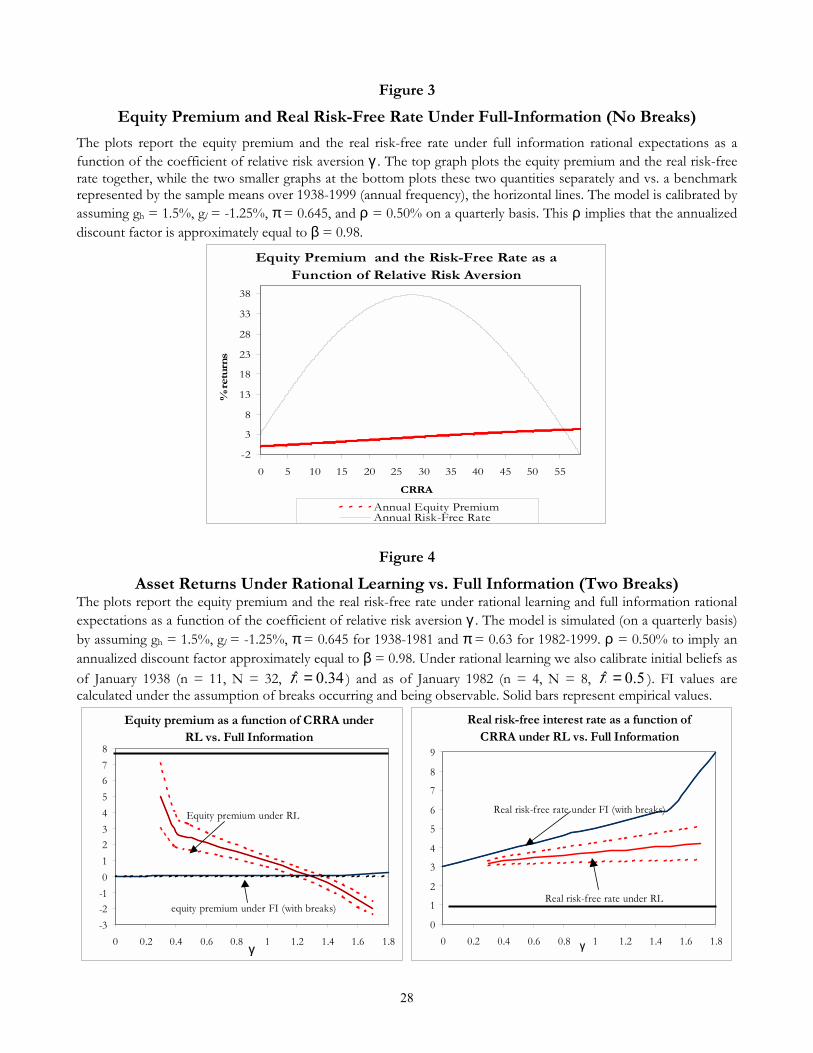
28

Figure 3

Equity Premium and Real Risk-Free Rate Under Full-Information (No Breaks)

The plots report the equity premium and the real risk-free rate under full information rational expectations as a function of the coefficient of relative risk aversion γ . The top graph plots the equity premium and the real risk-free rate together, while the two smaller graphs at the bottom plots these two quantities separately and vs. a benchmark represented by the sample means over 1938-1999 (annual frequency), the horizontal lines. The model is calibrated by assuming gh = 1.5%, gl = -1.25%, π = 0.645, and ρ = 0.50% on a quarterly basis. This ρ implies that the annualized discount factor is approximately equal to β = 0.98.

Equity Premium and the Risk-Free Rate as a Function of Relative Risk Aversion

-2

3

8

13

18

23

28

33

38

0 5 10 15 20 25 30 35 40 45 50 55

CRRA

% r

eturn

s

Annual Equity PremiumAnnual Risk-Free Rate

Figure 4

Asset Returns Under Rational Learning vs. Full Information (Two Breaks) The plots report the equity premium and the real risk-free rate under rational learning and full information rational expectations as a function of the coefficient of relative risk aversion γ . The model is simulated (on a quarterly basis) by assuming gh = 1.5%, gl = -1.25%, π = 0.645 for 1938-1981 and π = 0.63 for 1982-1999. ρ = 0.50% to imply an annualized discount factor approximately equal to β = 0.98. Under rational learning we also calibrate initial beliefs as of January 1938 (n = 11, N = 32, 34.0� =π ) and as of January 1982 (n = 4, N = 8, 5.0� =π ). FI values are calculated under the assumption of breaks occurring and being observable. Solid bars represent empirical values.

Equity premium as a function of CRRA under RL vs. Full Information

-3-2-1012345678

0 0.2 0.4 0.6 0.8 1 1.2 1.4 1.6 1.8γ

equity premium under FI (with breaks)

Equity premium under RL

Real risk-free interest rate as a function of CRRA under RL vs. Full Information

0

1

2

3

4

5

6

7

8

9

0 0.2 0.4 0.6 0.8 1 1.2 1.4 1.6 1.8γ

Real risk-free rate under RL

Real risk-free rate under FI (with breaks)

29

Figure 5

Volatility of Excess Equity Returns and Real Risk-Free Rate Under Rational Learning vs. Full Information (Under Two Breaks)

The plots report the standard deviation of excess equity returns and the real risk-free rate under rational learning and full information rational expectations as a function of the coefficient of relative risk aversion γ . The model is simulated (on a quarterly basis) by assuming gh = 1.5%, gl = -1.25%, π = 0.645 for 1938-1981, and gh = 1.5%, gl = -1.3%, π = 0.63 for 1982-1999. ρ = 0.50% on a quarterly basis. This ρ implies that the annualized discount factor is approximately equal to β = 0.98. Under rational learning we also calibrate initial beliefs as of January 1938 (n = 11, N = 32, 34.0� =π ) and as of January 1982 (n = 4, N = 8, 5.0� =π ). FI values are calculated by simulations under the assumption of breaks occurring and being observed.

Standard Deviation of Excess Equity Returns under RL vs. Full Information

02468

1012141618

0 0.2 0.4 0.6 0.8 1 1.2 1.4 1.6 1.8γ

Rational learning Full information

Standard Deviation of Real Risk-Free Interest Rates under RL vs. Full Information

-1-0.5

00.5

11.5

22.5

33.5

4

0 0.2 0.4 0.6 0.8 1 1.2 1.4 1.6 1.8γ

Rational learning Full information

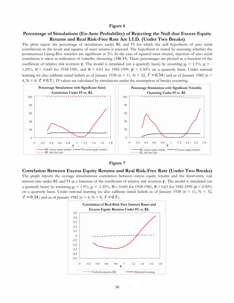
30

Figure 6

Percentage of Simulations (Ex-Ante Probability) of Rejecting the Null that Excess Equity Returns and Real Risk-Free Rate Are I.I.D. (Under Two Breaks)

The plots report the percentage of simulations under RL and FI for which the null hypothesis of zero serial correlations in the levels and squares of asset returns is rejected. The hypothesis is tested by assessing whether the portmanteau Lijung-Box statistics are significant at 5%. In the case of squared asset returns, rejection of zero serial correlation is taken as indication of volatility clustering (ARCH). These percentages are plotted as a function of the coefficient of relative risk aversion γ . The model is simulated (on a quarterly basis) by assuming gh = 1.5%, gl = -1.25%, π = 0.645 for 1938-1981, and π = 0.63 for 1982-1999. ρ = 0.50% on a quarterly basis. Under rational learning we also calibrate initial beliefs as of January 1938 (n = 11, N = 32, 34.0� =π ) and as of January 1982 (n = 4, N = 8, 5.0� =π ). FI values are calculated by simulations under the assumption of breaks occurring.

Percentage Simulations with Significant Serial Correlation Under FI vs. RL

0

20

40

60

80

100

0 0.2 0.4 0.6 0.8 1 1.2 1.4 1.6 1.8γ

RL excess equity returns FI excess equity returnsRL risk-free rate

Percentage Simulations with Significant Volatility Clustering Under FI vs. RL

0

20

40

60

80

100

0 0.2 0.4 0.6 0.8 1 1.2 1.4 1.6 1.8γ

RL excess equity returns FI excess equity returnsRL risk-free rate

Figure 7

Correlation Between Excess Equity Returns and Real Risk-Free Rate (Under Two Breaks) The graph reports the average simultaneous correlation between excess equity returns and the short-term, real interest rate under RL and FI as a function of the coefficient of relative risk aversion γ . The model is simulated (on a quarterly basis) by assuming gh = 1.5%, gl = -1.25%, π = 0.645 for 1938-1981, π = 0.63 for 1982-1999. ρ = 0.50% on a quarterly basis. Under rational learning we also calibrate initial beliefs as of January 1938 (n = 11, N = 32,

34.0� =π ) and as of January 1982 (n = 4, N = 8, 5.0� =π ).

Correlation of Real Risk-Free Interest Rates and Excess Equity Returns Under FI vs. RL

-0.5-0.4-0.3-0.2-0.1

00.10.20.30.40.5

0 0.2 0.4 0.6 0.8 1 1.2 1.4 1.6 1.8γ

Full information RE Rational learning

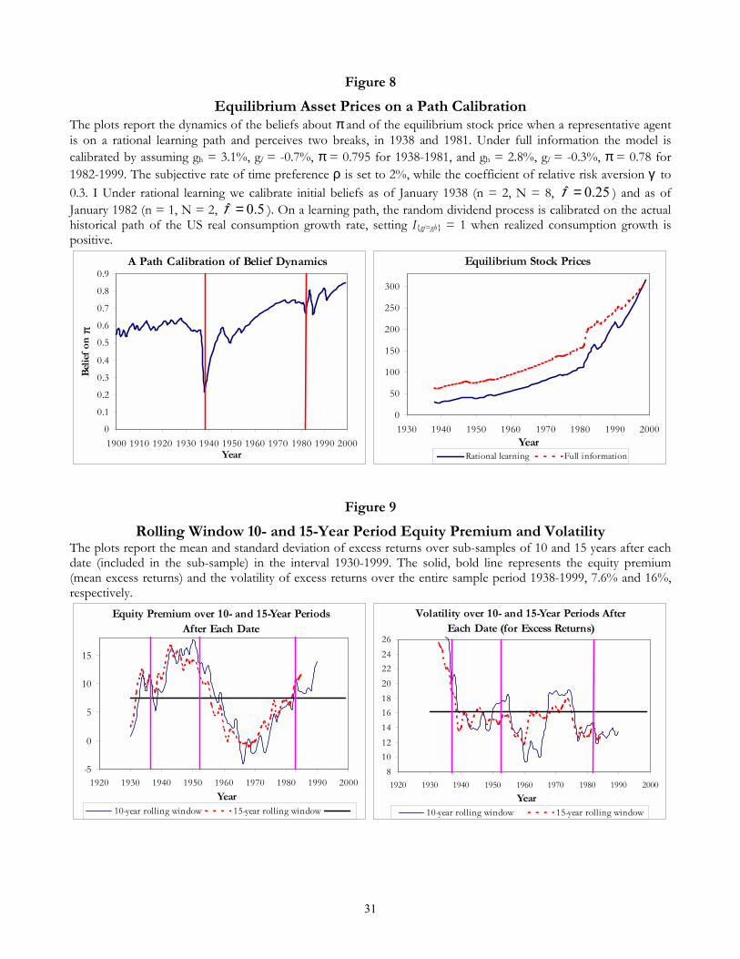
31

Figure 8

Equilibrium Asset Prices on a Path Calibration The plots report the dynamics of the beliefs about π and of the equilibrium stock price when a representative agent is on a rational learning path and perceives two breaks, in 1938 and 1981. Under full information the model is calibrated by assuming gh = 3.1%, gl = -0.7%, π = 0.795 for 1938-1981, and gh = 2.8%, gl = -0.3%, π = 0.78 for 1982-1999. The subjective rate of time preference ρ is set to 2%, while the coefficient of relative risk aversion γ to 0.3. I Under rational learning we calibrate initial beliefs as of January 1938 (n = 2, N = 8, 25.0� =π ) and as of January 1982 (n = 1, N = 2, 5.0� =π ). On a learning path, the random dividend process is calibrated on the actual historical path of the US real consumption growth rate, setting I{gj=gh} = 1 when realized consumption growth is positive.

A Path Calibration of Belief Dynamics

0

0.1

0.2

0.3

0.4

0.5

0.6

0.7

0.8

0.9

1900 1910 1920 1930 1940 1950 1960 1970 1980 1990 2000Year

Bel

ief

on π

Equilibrium Stock Prices

0

50

100

150

200

250

300

1930 1940 1950 1960 1970 1980 1990 2000Year

Rational learning Full information

Figure 9

Rolling Window 10- and 15-Year Period Equity Premium and Volatility The plots report the mean and standard deviation of excess returns over sub-samples of 10 and 15 years after each date (included in the sub-sample) in the interval 1930-1999. The solid, bold line represents the equity premium (mean excess returns) and the volatility of excess returns over the entire sample period 1938-1999, 7.6% and 16%, respectively.

Equity Premium over 10- and 15-Year Periods After Each Date

-5

0

5

10

15

1920 1930 1940 1950 1960 1970 1980 1990 2000Year

10-year rolling window 15-year rolling window

Volatility over 10- and 15-Year Periods After Each Date (for Excess Returns)

8101214161820222426

1920 1930 1940 1950 1960 1970 1980 1990 2000Year

10-year rolling window 15-year rolling window

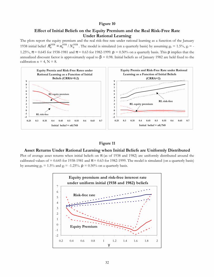
32

Figure 10

Effect of Initial Beliefs on the Equity Premium and the Real Risk-Free Rate Under Rational Learning

The plots report the equity premium and the real risk-free rate under rational learning as a function of the January 1938 initial belief 1938

019380

19380 /� Nn=π . The model is simulated (on a quarterly basis) by assuming gh = 1.5%, gl = -

1.25%, π = 0.645 for 1938-1981 and π = 0.63 for 1982-1999. ρ = 0.50% on a quarterly basis. This ρ implies that the annualized discount factor is approximately equal to β = 0.98. Initial beliefs as of January 1982 are held fixed to the calibration n = 4, N = 8.

Equity Premia and Risk-Free Rates under Rational Learning as a Function of Initial

Beliefs (CRRA=0.2)

-2 -1 0 1 2 3 4 5 6 7 8 9

0.25 0.3 0.35 0.4 0.45 0.5 0.55 0.6 0.65 0.7

Initial belief = n0/N0

RL equity premium

RL risk-free

Equity Premia and Risk-Free Rate under Rational Learning as a Function of Initial Beliefs

(CRRA=2)

-2-1012

3456789

0.25 0.3 0.35 0.4 0.45 0.5 0.55 0.6 0.65 0.7

Initial belief = n0/N0

RL equity premium RL risk-free

Figure 11

Asset Returns Under Rational Learning when Initial Beliefs are Uniformly Distributed Plot of average asset returns when initial beliefs on π (as of 1938 and 1982) are uniformly distributed around the calibrated values of = 0.645 for 1938-1981 and π = 0.63 for 1982-1999. The model is simulated (on a quarterly basis) by assuming gh = 1.5% and gl = -1.25%. ρ = 0.50% on a quarterly basis.

Equity premium and risk-free interest rate under uniform initial (1938 and 1982) beliefs

-2

-1

0

1

2

3

4

5

6

7

0.2 0.4 0.6 0.8 1 1.2 1.4 1.6 1.8 2γ

Risk-free rate

Equity Premium

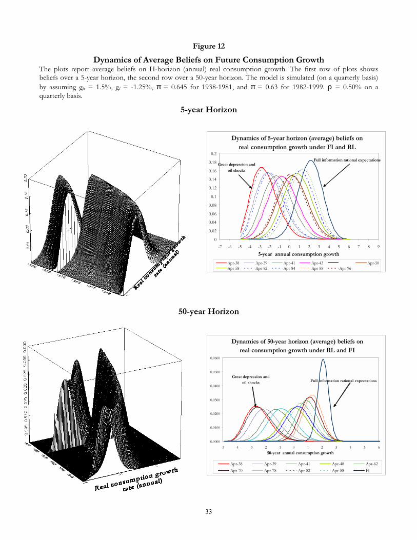
33

Dynamics of 5-year horizon (average) beliefs on real consumption growth under FI and RL

0

0.02

0.04

0.06

0.08

0.1

0.12

0.14

0.16

0.18

0.2

-7 -6 -5 -4 -3 -2 -1 0 1 2 3 4 5 6 7 8 95-year annual consumption growth

Apr-38 Apr-39 Apr-41 Apr-43 F I Apr-50Apr-58 Apr-82 Apr-84 Apr-88 Apr-96

Full information rational expectationsGreat depression and

oil shocks

Dynamics of 50-year horizon (average) beliefs on real consumption growth under RL and FI

0.0000

0.0100

0.0200

0.0300

0.0400

0.0500

0.0600

-5 -4 -3 -2 -1 0 1 2 3 4 5 650-year annual consumption growth

Apr-38 Apr-39 Apr-41 Apr-48 Apr-62Apr-70 Apr-78 Apr-82 Apr-88 FI

Full information rational expectationsGreat depression and

oil shocks

Figure 12

Dynamics of Average Beliefs on Future Consumption Growth The plots report average beliefs on H-horizon (annual) real consumption growth. The first row of plots shows beliefs over a 5-year horizon, the second row over a 50-year horizon. The model is simulated (on a quarterly basis) by assuming gh = 1.5%, gl = -1.25%, π = 0.645 for 1938-1981, and π = 0.63 for 1982-1999. ρ = 0.50% on a quarterly basis.

5-year Horizon

50-year Horizon