peydro, ma.; parres, f.; crespo amorós, je.; navarro vidal
TRANSCRIPT

Document downloaded from:
This paper must be cited as:
The final publication is available at
Copyright
http://dx.doi.org/10.1016/j.jmatprotec.2013.02.012
http://hdl.handle.net/10251/47988
Elsevier
Peydro, MA.; Parres, F.; Crespo Amorós, JE.; Navarro Vidal, R. (2013). Recovery ofrecycled acrylonitrile-butadiene-styrene, through mixing with styrene-ethylene/butylene-styrene. Journal of Materials Processing Technology. 213(8):1268-1283.doi:10.1016/j.jmatprotec.2013.02.012.

ABSTRACT
Recovery of recycled acrylonitrile–butadiene–styrene (ABS) through mixing with styrene-ethylene/butylene-styrene
(SEBS) has been studied in this paper. To simulate recycled ABS, virgin ABS was processed through 5 cycles, at
extreme processing temperatures, 220 ºC and 260 ºC. The virgin ABS, the virgin SEBS, the recycled ABS and the
mixtures were mechanically, thermally and rheologically characterized after the various cycles of reprocessing in order
to evaluate their corresponding properties and correlate them with the number of cycles undergone. With these data and
using CAE (Computer Aided Engineering) the injection process was simulated by obtaining the optimal injection
process parameters. Mixtures were injected at two temperatures in a sensorised mold correlating the shrinkage of the
parts with temperature.
The results show that tensile strength of ABS remains practically constant as the number of reprocessing cycles
increases, while in the material injected with SEBS the tensile strength decreases. Concerning the Charpy notched
impact strength; the values of the ABS reprocessed at 220 ºC remain more or less unchanged, while the values for 260
ºC show a significant decrease. The adhesion of the SEBS causes, in both cases, an increase in impact strength. DSC
techniques enabled us to observe how the glass transition temperature (Tg) remains more or less constant regardless of
the number of cycles or the temperature, whereas the crosslinking is much greater in the samples reprocessed at 260 ºC.
Finally, the viscosity decreases with each cycle and this decrease becomes even more noticeable with the addition of
SEBS, and also that the parts molded at lower temperatures have less shrinkage.
KEYWORDS
Degradation, Recovery, ABS, SEBS, Injection, Shrinkage.

1. INTRODUCTION
The current economic crisis has led to an increase in competition between companies, who in turn have had to
significantly reduce production costs in order to remain competitive. These reductions must be found in areas such as
raw materials, waste reduction, process optimization, etc. In the case of companies who transform polymer materials,
the economic crisis, alongside a dependence on the price of petroleum, have led many companies to use recycled
materials to obtain raw materials at a more stable price. There is also the added incentive of the environmental benefits
gained by reusing waste materials.
One of the most important conditioning factors when substituting a virgin material for a recycled material is the
question of whether the original characteristics are preserved in the recycled material. A disadvantage of thermoplastics
is the variation in their properties, not only due to the effect of successive thermal processes, but also due to their
exposure to atmospheric phenomena. Balart et al. (2005) studied the properties of Acrylonitrile–butadiene–styrene
(ABS) derived from the electrical and electronic sector, to be more precise, from streetlights. These pieces are
extremely exposed to atmospheric phenomena. Balart improved the properties of the waste material by mixing it with
polycarbonate (PC) and then studied the miscibility of the mixture. Another author, Liu et al. (2002) obtained similar
results using Polyamide (PA). This variation in properties has been rectified by various authors through the use of
additives or even by adding other polymers. For example, Tasdemir (2004) used styrene-butadiene-styrene (SBS) and
Tasdemir and Karatop (2006) styrene-isopren-styrene (SIS) also as compatibilizers in mixtures of ABS/PC. SBS and
SIS are materials that are very common in SEBS, but there appear to be no studies into incorporation of SEBS in
recycled polymers in order to recover their properties. Other examples are those of Li et al. (2010), who studied
mixtures of PPO/PA with SEBS-g-MA and ABS-g-MA and Yin et al. (2007), who studied mixtures of PC/SAN with
SEBS. These studies are not comparable to our own as other materials were used, however, they show that there is an
improvement in properties with the addition of SEBS to the materials used.
ABS is a technical thermoplastic that is widely used in a range of industries, such as the automobile, electrical,
electronic, etc. sectors. Its main advantage is the good relationship between price and performance, although the
presence of a polybutadiene phase brings certain problems when it is submitted to various processing cycles, either by
injection or extrusion. The studies carried out by Bai et al. (2007), Boronat et al. (2009), Karahaliou and Tarantili,
(2009) and Perez et al. (2010) clearly demonstrate this. Nearly all studies in this area highlight the crosslinking
phenomena as the cause of the variation in properties that takes place (loss of ductility). In previous studies, such as
those of Tasdemir (2004) and Tasdemir and Karatop (2006), SBS, SIS and styrene-butadiene rubber (SBR) have been
used with the aim of recovering the ductility that is lost in some polymers, but the use of these polymers may cause
crosslinking in future reprocessing cycles as in all cases there is a double C=C.

One of the fundamental properties to consider when studying polymer processing is its rheological behavior.
Understanding this parameter is vital to carry out a correct extrusion or injection of the polymer. The real viscosity of a
polymer is obtained using a capilliary rheometer along with the Bagley and Rabinowitsc corrections. The methodology
used in this work to calculate the viscosity is the same as used by Peydro et al. (2011) in his study of HIPS, which is
comprehensively explained in that work.
Some injection processing simulations, such as Autodesk Moldflow Inside 2012 ®, use values of the parameters from
the Cross-WLF model. Cross (1965) and Williams et al. (1955) carried out experiments to reproduce the rheological
behavior of the materials during the injection process. Reig in his works (2005) and (2007), and Boronat et al. (2009),
applied these models in their studies on reprocessed ABS + PC and ABS respectively. Reig in his 2007 work
determined a Material Processability Index (MPI) from three mixtures of ABS + PC with a different Melt Flow Index
(MFI). Reig calculated the Cross parameters for each mixture and uses the methodology for the design of experiments
(DOE). The variables reused in the DOE were the variables from injection processing (filling time, melt temperature,
coolant temperature, packing pressure level and filling-packing switch-over). For all of this, Reig used the computer
simulation of the injection process to determine that the ideal PC content in the ABS/PC blend is 3.6 %.
Boronat´s study is interesting because he calculated the Cross dependant parameters of his mixtures and shows how
variations in these affect viscosity. At the same time, he showed that increasing the temperature has a greater influence
on the degradation of ABS than increases in the shear rate.
Boronat´s study is very interesting for us because it calculates the dependent Cross parameters of mixtures and indicates
how they affect the viscosity variation of each. This study in turn proves that the increase in temperature has more
influence on the degradation of ABS than increasing the shear rate.
Other interesting studies are those by Shin and Park (2009) and Ozcelik and Sonat (2009) both of whom used the
Moldflow ® simulation to study two real cases. The first is focused on breakages in ice machine parts. Shin concludes
that the failure occurs by residual stress in the end part originated from high injection pressure. The second examines
the thin shell cell phone cover. Ozcelik calculates the best point of injection and the machine parameters that produce
less distortion of the piece.
Hot-melt polymers shrink when injected into the cold mold cavity. In the injection molding process, pressure is high
near the polymer entrance and low at the last-fill location. The polymer temperature is low near the mold wall surface
and high in the core region. Because of these two types of non-uniformity, the part will shrink differently at different
planar and thickness locations, which causes warpage.

Finally, the study by Chang and Faison (2001) is very interesting for us, as he uses Dr. C-Mold ® for simulations and
experiments with contractions that are longitudinal and transverse to the flow. However, this study does not take into
account that the transverse contraction is not the same close to the entry point as it is farther away from this point.
A major objective of this work is to study the process of recycling ABS in its two stages: firstly, at the stage of
reprocessing from virgin status until its fifth reprocessing cycle, and secondly, in the recovery phase of properties by
incorporating SEBS, analyzing mechanical, thermal and rheological properties.
Another objective is to determine model parameters of both the Cross-WLF virgin material as well as the recycled and
mixed materials, in order to implement them in the plastic injection simulation.
The ultimate goal is to measure the shrinkage of the parts correlating with the measured pressure in the mold sensorised
and the injection temperature.
2. EXPERIMENTAL
2.1. Material
The ABS and SEBS used in the experiments are commercial products; ABS Terluran GP 35® (BASF, Ludwigshafen,
Germany) and SEBS Megol TA 50 ® (Applicazioni Plastiche Industriali, Mussolente, Italy). Table 1 shows fresh
material used in this study.
Table 1. Mechanical characterization values of the virgin ABS and virgin SEBS.
Material
Tensile strength
(MPa)
Elongation at
break (%)
Charpy notched
impact strength
(kJ·m-2)
Hardness
Source
ABS 44 12 19 75 (Shore D) BASF
SEBS 6.0 600 - 50 (Shore A) API
2.2. Preparation of samples
The degradation process was conducted with a conventional injection machine (Meteor 270/75 de Mateu & Solé®
(Barcelona, Spain)) at two injection molding temperatures (220 ºC and 260 ºC), which represent the upper and lower
recommended values for ABS processing. This process was repeated until five cycles were completed. Prior to the

injection process each of the samples was dried at 80 ºC in a dehumidifier (MDEU1/10 de Industrial y Comercial Marse
S.L.®, Barcelona Spain).
The mixtures of degraded ABS and SEBS were obtained using a twin screw extruder at a maximum temperature of 220
ºC and varying the percentage of SEBS (0, 2.5, 5, 10 % by weight).
As there was a range of samples in the experiments, we used the code shown in Table 2. For example, R5_260_2.5. 5
represents 5 recycling cycles at 260 ºC mixed with 2.5 % SEBS.
Table 2. Samples code.
Material Nº of cycles Processing
temperature
% of SEBS
R (Reprocessed) 1 220 0
2 260 2.5
3 5
4 10
5
2.3. Mechanical characterization
Mechanical properties of ABS, reprocessed ABS and ABS-SEBS were obtained with a universal tensile test machine
ELIB 30 by S.A.E. Ibertest® (Madrid, Spain) following the guidelines of ISO 527. All samples were 150 mm long and
10•4 mm2 area, and were tested at 25 ºC and a relative humidity of 50 % using a crosshead rate of 50 mm min-1 with a
load cell of 5KN. A minimum of ten samples were tested and average values of elongation at break (ductile mechanical
property) and tensile strength (mechanical resistance property) were calculated.
The impact test was carried out using the Charpy axial impact pendulum (Metrotec®, San Sebastián, Spain) with
adjustable masses for energy ranges of 1 and 6 J according to ISO 179.
Hardness of materials was determined using a shore hardness meter by J. Bot Instruments S.A.® (Barcelona, Spain)
with the D scale following the guidelines of ISO 868.
2.4. Thermal characterization
ABS degradation and miscibility of the different components of ABS/SEBS system was studied through the changes in
glass transition temperature (Tg), crosslinking temperature and crosslinking enthalpy using a Mettler-Toledo 821 DSC
(Mettler Toledo Inc.™ , Schwarzenbach, Switzerland). 9–11 mg samples were subjected to a first heating (30–110 ºC at

10 ºC/min) followed by a slow cooling to remove thermal history and were heated again (30– 300 ºC at 10 ºC/min) until
degradation. Measurements of glass transition temperature, crosslinking temperature and crosslinking enthalpy were
taken on the second heating curve.
2.5. Rheological characterization
The rheological analysis of all the materials was done using a Thermo Haake Rheoflixer MTVR capillary Rheometer by
ThermoHaake (Dieselstr – Karlsruhe, Germany). The temperatures used in the rheometer were 220 ºC and 260 ºC for
ABS, for both cycles of reprocessing (220 ºC and 260 ºC) and its Blends. For SEBS temperatures of 180 ºC and 200 ºC
were used. To get a complete and accuracy rheological characterization of the samples, these have been tested at two
temperatures. The shear rates used in the study were in the range 100 to 10,000 s-1. The rheometer was equipped with
three separate dies, all with a diameter of 1 mm and with L/D ratios of 10, 20, and 30. The barrel pressure and ram rate
were converted into real shear stress (τ) and shear rate (γ), respectively, using Bagley and Weissenberg–Rabinowitsch
corrections. The tests were carried out in compliance with ISO 11443. The viscosity values correspond to the average of
the five experimental tests. The residence time in the rheometer was 5 minutes. Figure 1 shows the Rheological curves
virgin ABS at 220 ºC and 260 ºC and virgin SEBS at 180 ºC and 200 ºC.
Figure 1. Rheological curves virgin ABS at 220 ºC and 260 ºC and virgin SEBS at 180 ºC and 200 ºC.
2.6. Simulation of the injection mold
The injection simulation analyses were calculated using the computer-aided engineering Autodesk Molflow Insight
(version 2012) ® software. The simulation results were used to determine the best injection conditions at extreme
temperatures of 220 °C and 260 °C. Figure 2 shows the geometry used in this study. It is a thin flat rectangular cavity

of 160·60·2 mm3. The samples were injected into a mold equipped with two pressure sensors and two thermal sensors.
The pressure sensors, model Kistler 6157BA, were placed in the bottom of the sprue and in the entrance of the cavity
next to a thermal sensor, model Kistler 6192A. The other thermal sensor was in the other end of the cavity as shown in
Figure 2.
Calculated pressures in the mold were compared with those obtained in the simulation. The mold temperature was
maintained at 50 ° C for all tests. As there were a number of samples, to identify the point where pressure is measured,
the coding shown in Table 2 was used (adding a P1 or P2, depending on whether a point is at the bottom of sprue or at
the entrance of the cavity respectively). For example: R4_260_2.5_P1.
Also the simulated contraction of the samples was compared to the measurement taken with a micrometer TESA ®
(Renens, Switzerland) for a measuring range of 150-175 and Kalkum Ezquerra ® (Los Fresnos - Haro - La Rioja,
Spain) for a measuring range of 50 -75, both of 0.001 mm precision.
Figure 2. Geometry of injected part and position of pressure and temperature sensors.
3. METHODOLOGY
3.1. Methodology for viscosity calculation using cross-wlf model.
Capillary rheology was used for rheological characterization of virgin and reprocessed material. Extrusion rheometry
was selected because the shear rate range studied includes injection shear rates. To get a complete rheological
characterization of the samples, these were tested at two temperatures, 220 °C and 260 °C, which coincide with the
processing temperature limits according to the manufacturer. The barrel pressure and ram rate were converted into real
shear stress (τ) and shear rate ( ), respectively, using Bagley and Weissenberg–Rabinowitsch corrections. The
viscosity was calculated with the quotient between shear stress and shear rate, as seen in equation (1). As with the
calculation of viscosity, three dies were used, and three viscosity curves were obtained for each material.
(1)
Cross model (1965), equation (2), has been chosen to assess the viscosity of the material because it is the most
appropriate model to study both filling and packing phases.
This method also allows calculation of viscosity of the material at any temperature from a viscosity curve at a given
temperature.
n
1
*0
0
1 (2)
Where η0 [Pa·s] is material viscosity under zero-shear-rate conditions, τ* [Pa] is the model constant that shows the
shear stress rate, from which the pseudoplastic behavior of the material starts, n [−] is the model constant which
symbolizes the pseudoplastic behavior slope of the material as: (1−n).
To determine the viscosity of the material with zero shear, we used the Williams-Landel-Ferry (1955) expression (3).
1
2
0 1
A T T
A T TD e
, si T ≥ T o η0 = ∞ , si T ≤ T (3)
2 2 3A A D p
pDDT 32
~
Where T [K] is the glass transition temperature of the material, depending on the pressure, D2 [K] is the model constant
which registers the glass transition temperature of the material at atmospheric pressure, D3 [K/Pa] is the model constant
which symbolizes the variation of the glass transition temperature of the material, according to the pressure,D1 [Pa s] is
the model constant which registers the material viscosity, under zero shear rate conditions, at material glass transition
temperature and at atmospheric pressure,A1 [−] is the model constant that shows the temperature dependence of material
glass transition temperature under zero shear rate conditions and Ã2 [K] is a model parameter that depends on the type
of material that has been considered.

The independent parameters of the Cross model are those which only depend on the material and which were
obtained from Moldflow 6.1 ® simulation data and from the DSC Figure 4a. Ã2 = 51.6 K. D2, = Tg = 105 ºC = 378.15
K. p
TD g
3 = 0 K/Pa
The dependent parameters of the Cross model which must be calculated are: n [-]; τ* [Pa]; D1 [Pa·s]; A1 [-].
In order to calculate these parameters we used the MathCad 2001 ® program for the interaction, using data from the
three dies.
Once the parameters were obtained, they were introduced into the data base of Autodesk Molflow Insight (2012) ® in
order to then obtain the material viscosity graphics. Figure 3 shows the viscosity of virgin material at five different
temperatures.
Figure 3. Viscosity of virgin material at 200, 220, 240, 260 and 280 ºC.
3.2. Methodology for determination of specific heat capacity (cp).
The sapphire method for cp determination has been used for more than 30 years. The DSC signal of the sample is
compared with the DSC signal of the calibration sample for known specific heat. Both curves are blank curve corrected
(automatic blank curve correction). A total of three measurements are made: blank (empty crucible), sapphire (3 small
sapphire disks of 4.8 mm diameter, as in the calibration sample) and the sample itself. A blank curve correction is, in
this case, also essential.

1) Blank run (empty pans in sample and reference holders);
2) Calibration run (calibration material in sample holder pan and empty pan in reference holder);
3) Specimen run (specimen in sample holder pan and empty pan in reference holder).
blankrunnruncalibratio
sp
blankrunnspecimenrucal
calp
spp PPm
PPmcc
(4)
Once the DSC graphs are obtained and processed, see Figure 4a, the calibration cp is needed, in this case sapphire and
formula (4) is applied. Finally, the graph shown in Figure 4b is obtained.
The data on specific heat capacity of virgin material, in the simulator database, has an approximate value in this case of
2,155 J/(kg ºC) for 200 ºC. After calculation, a value of 2850 J/(kg ºC) was obtained for virgin material and 2904 J/(kg
ºC) for recycled material.
Figure 4. Calorimetric curve of virgin ABS and R5. Cp of sapphire, virgin ABS and R5.
3.3. Methodology of the simulation system
Injection simulation is a useful tool because it can detect design errors in the parts before making the mold. It is also
very useful because it predicts the approximate values of the injection parameters to be introduced in the injection
molding machine, allowing the size of the injection molding machine to be selected beforehand and therefore allowing
production costs to be estimated.
Before starting the simulation, all injection data for the new materials characterized was introduced into the simulator.
These data are the dependent parameters of the Cross-WLF model and specific heat capacity.

There follows an explanation of the methodology used for the simulation of virgin materials. For all other materials the
methodology is identical.
The first step was the simulation of the filling phase. Several simulations were made at different injection times until
the optimum injection conditions were identified. Table 3 shows the results of the simulation processes in the filling
phase for comparison.
Table 3. Results of the simulation process.
Simulations 1st 2nd 3rd 4th 5th 6th
Injection temperature (ºC) 220 220 220 260 260 260
Injection time (s) 1.0 1.3 1.5 0.5 0.8 1.1
Maximum clamp force (tons) 20.82 21.08 22.36 13.75 13.95 14.31
Maximum injection pressure (MPa) 94.52 96.55 97.81 71.75 69.11 69.53
Maximum shear rate (1/s) 3,881 2,987 3,235 9,361 4,658 3,842
Maximum shear stress (MPa) 0.34 0.3 0.31 0.26 0.20 0.20
Maximum temperature position part (ºC) 235.5 234.5 234.3 275 271.4 270.6
Maximum difference temperature at flow front (ºC) 3.8 5.0 5.4 1.5 3.1 3.5
When analyzing Table 3, it can be observed that for the simulations at 220 °C, the 2nd simulation is the only one that
does not exceed the limit of maximum 0.3 MPa of shear stress, as specified by the manufacturer. In the simulations at
260 °C, the 5th cycle presents the injection pressure and shear stress and the second lowest minimum closing force.
Thus, the Fill time was set at 1.3s for injection at 220 °C and 0.8 s at 260 °C.
The second step was the simulation of the packing phase. In our case, first of all, injections were carried out using a
machine to identify the limits. It was discovered that it was necessary to reduce the packing pressure to 80% of the
maximum pressure reached in the filling at 220 ° C and 70% at 260 ° C. If this is not done, the mold opens, with the
consequent appearance of flash in the part. Furthermore, the filling-packing switch-over was set at 95% of the stroke.
Figure 5 shows the pressure versus time cycle for the simulation of injection at 220 °C, at the two points studied (sprue
- P1 and part - P2). These points are where the sensors are located in the mold. A peak sprue point of maximum
pressure 82.13 MPa and 73.04 MPa (packing) can be seen. In contrast, at the point of the piece (P2), a peak of 53.57
MPa was observed in the packing phase.

Figure 5. Pressures obtained in the simulator by injecting at 220 °C with virgin material.
The third step was to simulate the cooling phase. For the simulation at 220 °C, Figure 6 shows the graph of
temperature points studied (1 and 3) as well as the entry point (point 2). It emphasizes that after 11 seconds
(corresponding to a compaction of 10 seconds) the temperature of the entry point is below 105 °C (glass transition
temperature) and therefore, the material can be more compacted. It is also noted that on after 15 seconds, the piece
(point 3) is also below 85 °C (ejection temperature) and can be removed. From these data it follows that the cooling
time has to be 15 seconds. However, from the machine experiment, it was observed that the minimum time needed for
the shot is around 5 seconds. Therefore, the mold close time has to be 5 seconds, which is added to the fill and packing
time (11 seconds) to obtain a cooling time of 16 seconds. The part can be ejected although the sprue temperature (point
1) is above the ejection temperature. This is not important, as the sprue is residue and it is not important if it is not
correctly injected.
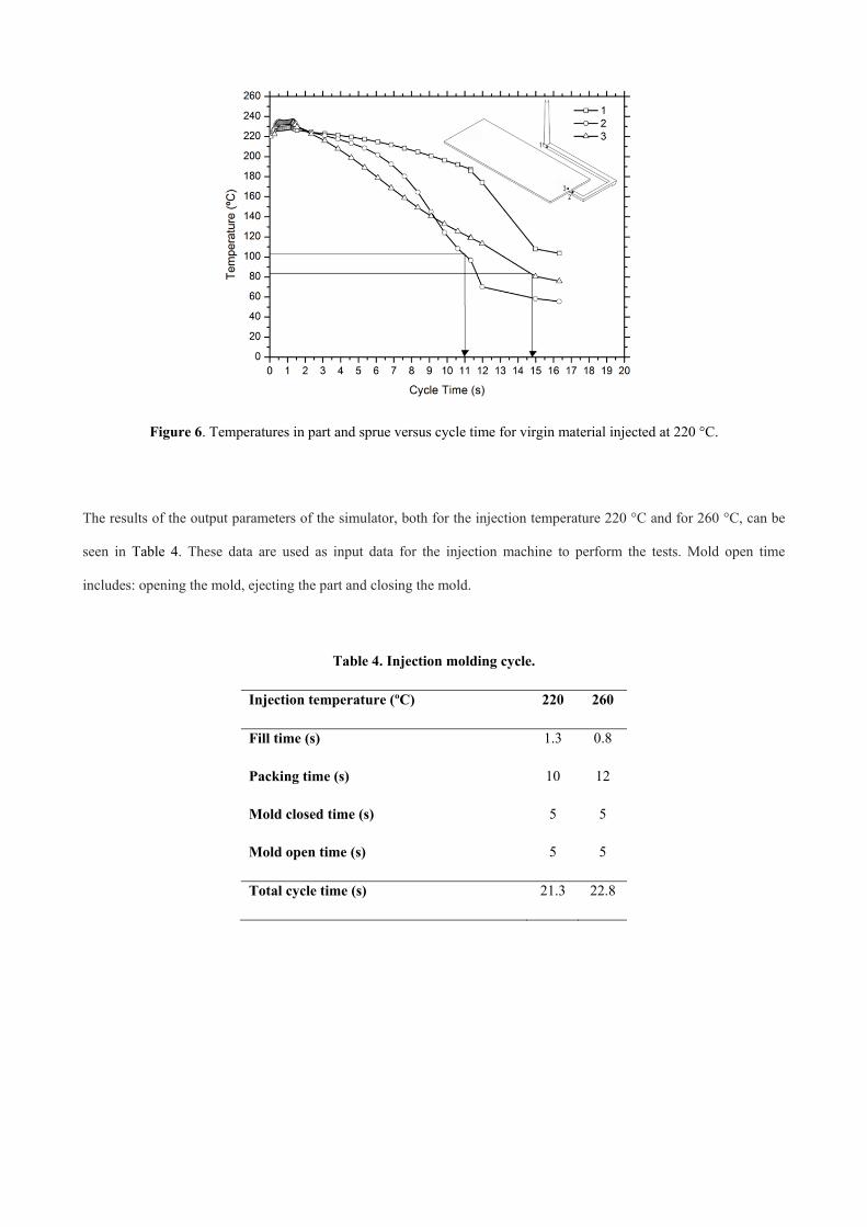
Figure 6. Temperatures in part and sprue versus cycle time for virgin material injected at 220 °C.
The results of the output parameters of the simulator, both for the injection temperature 220 °C and for 260 °C, can be
seen in Table 4. These data are used as input data for the injection machine to perform the tests. Mold open time
includes: opening the mold, ejecting the part and closing the mold.
Table 4. Injection molding cycle.
Injection temperature (ºC) 220 260
Fill time (s) 1.3 0.8
Packing time (s) 10 12
Mold closed time (s) 5 5
Mold open time (s) 5 5
Total cycle time (s) 21.3 22.8

4. RESULTS AND DISCUSSION
4.1. Characterization of degraded ABS over various injection cycles
4.1.1. Mechanical properties
The mechanical properties of any material are fundamental for its use in any particular application. Traction and impact
test are extremely important because they allow us to understand properties such as tensile strength, elongation at break
and impact strength.
Table 5 shows the values obtained from the mechanical characterization of ABS in function of the number of cycles,
both at 220 ºC and 260 ºC. A high level of stability in the ABS was observed after successive injection cycles; the
tensile strength and elongation at break values remained virtually constant. This behavior has been observed by a
number of other authors such as Bai et al. (2007), Eguiazabal and Nazabal (1990), Perez et al. (2010) and Salari and
Ranjbar (2008). However, different impact strength values for the two temperatures (220 and 260 ºC) were obtained. In
the first case (220 ºC), impact energy remains more or less constant, but the values fall when the temperature used is
260 ºC. This phenomena was also observed by Bai et al. (2007) and Eguiazabal and Nazabal (1990). This decrease is
due to the crosslinking phenomenon arising from the break in C=C double bond, which limits the later use and
application of the recycled ABS.
Previously, results show that the 220 ºC temperature is better than 260 ºC, but the injection process is slower and more
injection pressure is needed due to the higher viscosity shown by the ABS at 220 ºC.
Table 5. Mechanical characterization values of the reprocessed ABS at 220 ºC and 260 ºC.
Temperature (ºC)
Material (cycles)
Tensile strength (MPa)
Elongation at break (%)
Charpy notched impact strength
(kJ·m-2)
Hardness (Shore D)
ABS V 40.96±0.54 9.64±0.32 18.43±0.16 75.5±1.87
220 1 41.58±0.56 8.57±1.06 18.32±0.41 76.0±0.35
2 40.93±0.38 8.38±1.23 18.33±0.17 75.6±0.89
3 41.83±0.23 8.48±0.92 18.85±0.17 74.9±2.13
4 41.28±0.47 7.75±0.28 18.95±0.29 75.9±1.14
5 41.10±1.07 8.93±0.76 17.91±0.17 75.6±0.89
V 40.96±0.54 9.64±0.32 18.43±0.16 75.5±1.87
260 1 41.12±0.94 8.54±1.73 18.50±0.14 74.6±0.89
2 41.32±0.43 7.47±1.60 17.35±0.85 75.8±3.11
3 41.65±0.65 7.38±0.46 14.98±0.48 75.7±0.44
4 41.68±0.54 9.07±1.00 12.59±0.33 75.6±0.65
5 41.95±0.37 7.20±0.50 11.68±0.87 77.0±1.41
SEBS V 6.0 600 - 50 (Shore A)
4.1.2. Thermal analysis
Differential scanning calorimetry (DSC) shows the different thermal transitions that take place in a polymer, such as
glass transition temperature (Tg), melt point temperature (Tm) and initial degradation temperature (Tz).Although it is also
possible to observe other phenomena, such as cold crystallization, which is typical in PET, studied by Flores (Flores et
al., 2008), and crosslinking reactions due to the presence of double carbon bonds. This reaction has been calculated with
the integral of the curve in the zone of the peak, (onset: 225.83 ºC, enset: 250.55 ºC). Figure 4a shows the thermal
curve of virgin ABS, and here we can see the Tg of the styrene phase and the crosslinking of the polybutadiene phase.
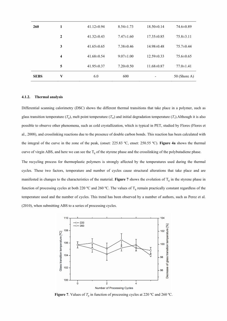
The recycling process for thermoplastic polymers is strongly affected by the temperatures used during the thermal
cycles. These two factors, temperature and number of cycles cause structural alterations that take place and are
manifested in changes to the characteristics of the material. Figure 7 shows the evolution of Tg in the styrene phase in
function of processing cycles at both 220 ºC and 260 ºC. The values of Tg remain practically constant regardless of the
temperature used and the number of cycles. This trend has been observed by a number of authors, such as Perez et al.
(2010), when submitting ABS to a series of processing cycles.
Figure 7. Values of Tg in function of processing cycles at 220 ºC and 260 ºC.

However, the crosslinking reaction in the polybutadiene phase does cause changes in the values, both at 220 ºC and 260
ºC. In both cases, the crosslinking enthalpy value decreases in function of processing cycles, but this decrease is much
more marked for the samples at 260 ºC. This is because the crosslinking process is irreversible and takes place between
approximately 220 ºC and 260 ºC. In the reprocessing of the material at 220 ºC, these temperatures are hardly reached,
which means that only a small quantity of double links reacts in each cycle. However, for the reprocessing at 260 ºC,
the reaction is produced in the first and second reprocessing, with no remaining double links left to react in the
successive cycles, (Figure 8).
Figure 8. Crosslinking enthalpy in function of reprocessing cycles at 220 ºC and 260 ºC.
4.1.3. Analysis of rheological properties.
One of the fundamental properties to consider when studying polymer processing is its rheological behavior.
Understanding this parameter is vital to carry out a correct extrusion or injection of the polymer. In order to achieve a
complete rheological characterization of the samples, they were subjected to capillary rheometer tests at 220 ºC and
260 ºC.
Table 7 shows the values of the Cross-WLF model and the viscosity of the material at zero shear rate at temperatures of
220 ºC and 260 ºC. These values are very important in enabling us to carry out an accurate injection simulation using
data on reprocessed material, given that no other data base exists.
To calculate these parameters, we used the Math-Cad 2001 ® program for the interaction and used data from the three
dies. The equation for this calculation can be seen in Eq. (5).
ChiCuadrado D1 A1 n datos 0
rows datos( ) 1
i
datosi 2 datos
i 0 datosi 1 D1 A1 n 2
datosi 0 datos
i 1 D1 A1 n
(5)
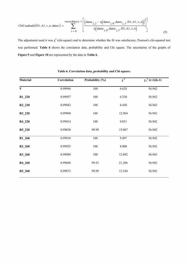
The adjustment used it was χ2 (chi-square) and to determine whether the fit was satisfactory, Pearson's chi-squared test
was performed. Table 6 shows the correlation data, probability and Chi square. The uncertainty of the graphs of
Figure 9 and Figure 10 are represented by the data in Table 6.
Table 6. Correlation data, probability and Chi square.
Material Correlation Probability (%) χ 2 χ t2 (r-1)(k-1)
V 0.99944 100 6.628 56.942
R1_220 0.99957 100 6.530 56.942
R2_220 0.99943 100 8.450 56.942
R3_220 0.99908 100 12.964 56.942
R4_220 0.99914 100 9.851 56.942
R5_220 0.99838 99.99 15.067 56.942
R1_260 0.99918 100 9.497 56.942
R2_260 0.99935 100 8.008 56.942
R3_260 0.99989 100 12.092 56.942
R4_260 0.99688 99.53 21.286 56.942
R5_260 0.99873 99.99 13.244 56.942

Table 7. Dependent parameters of the Cross-WLF model.
Material n (-) * (Pa) D1 (Pa·s) D2 (ºC) D3 (K/Pa) A1 (-) Ã2 (K) 0 (Pa/s) 0 (Pa/s)
220 ºC 260 ºC
V 0.23493 81,101 2.33693·1011 378.15 0 25.96 51.6 3,855.0 812.7
R1_220 0.24513 73,057 1.44613·1011 378.15 0 25.10 51.6 4,325.3 960.2
R2_220 0.25578 67,698 7.4067·1011 378.15 0 27.39 51.6 4,547.3 879.8
R3_220 0.26693 60,166 1.01513·1012 378.15 0 27.68 51.6 5,110.6 971.8
R4_220 0.25071 72,508 1.9747·1011 378.15 0 25.69 51.6 3,922.9 840.5
R5_220 0.25999 68,512 1.68448·1011 378.15 0 25.46 51.6 3,920.8 851.7
R1_260 0.25629 71,543 5.23962·1011 378.15 0 27.10 51.6 3,940.9 776.0
R2_260 0.25184 73,316 3.26807·1011 378.15 0 26.40 51.6 3,985.9 818.5
R3_260 0.26261 68,648 5.61485·1011 378.15 0 27.15 51.6 4,081.8 801.4
R4_260 0.27416 65,688 6.07148·1011 378.15 0 27.35 51.6 3,848.6 746.7
R5_260 0.25142 82,034 3.11695·1011 378.15 0 26.69 51.6 3,114.7 628.7
The variation in the value n (a constant of the model represented as (1-n) which describes the pseudoplastic behavior of
the material) increases slightly with each new reprocessing cycle, at both 220 °C and 260 °C. This slight increase in n
causes a slight reduction in the slope. This slight reduction in the slope of the curve causes a slight increase in viscosity
under the same conditions of zero shear rate.
The variation of the value which shows the shear stress rate at which the pseudoplastic behavior of the material
begins, diminishes slightly with each cycle. This behavior causes the viscosity curve to move to the left, causing a slight
reduction in viscosity.
The parameter D1 (a constant of the model which shows the viscosity of the material at zero shear rate conditions, and
at the transition temperature and atmospheric pressure) and the parameter A1 (a constant of the model which shows the
sensitivity of the viscosity at zero shear rate at the temperature) are not represented as the model developed with
MathCad 2001 ® can give the same viscosity values for different pairs of D1 and A1.
The variation in the value η0, viscosity of the material at zero shear rate, for both test temperatures (220 °C and 260 °C),
can be seen in Table 7. This value remains more or less constant temperature of 220 °C, however, for the temperature

of 260 °C and reprocessing at 260 ºC it shows a slight decline as the number of cycles increases. For a temperature of
260 °C and reprocessing at 220 °C this value remains more or less constant.
Viscosity curves, Figure 9, have been obtained replacing the data of Table 7 in Equation 2. The rheological behavior of
reprocessed materials at both 220 °C (Figure 9a) and 260 °C (Figure 9b) is virtually the same. When the material is
heated at low temperatures, 220 °C, increasing n (which decreases the slope of the curve) and decreasing (which
shifts the curve to the left) causes the curves to intersect at the average shear rates (above 2000 s-1) zone. This
intersection of curves leads to a slight drop in viscosity at low shear rates and a very slight increase in viscosity to high,
as the material is reprocessed.
Figure 9. Viscosity of virgin and reprocessed material at 220 ºC and 260 ºC.
When the material is heated to high temperatures, 260 °C, the variation of n and * cause the curves to converge in the
area of high shear rates. There is a slight decrease in viscosity at low shear rates, but values remain constant at high

rates as the material is reprocessed. This viscosity change is easier to see when looking at the viscosity values for low
shear rates (100s-1) Figure 10a and high shear rates (5,000 s-1) Figure 10b.
The study of polymer viscosity at low and high shear rates is very important since during the injection process the shear
rate occurs in both the fill phase (high shear rate) and in the packing phase (low shear rate). Navarro et al. (2008) in his
work mentions the importance of studying these two stages of injection separately.
Figure 10.Viscosity of virgin and reprocessed material at shear rate of 100 and 5,000 s-1.
Viscosity is a property that is extremely sensitive to variations in molecular weight. This behavior which sees falls in
viscosity at low shear rates is due to degradation of the material (breaks in the polymer chains which then become

shorter), as the material is repeatedly reprocessed (injected and pelletized) and because of the temperature and shear that
occur in the injection process.
Similar results have been obtained by other authors, such as Boronat et al. (2009) who observed with a low viscosity
ABS (like ours) the same effect, ie a fall in viscosity at low shear rate only.
4.1.4. Analysis of the pressures in the mold.
The quality of injection-molded parts is largely decided within the mold. The cyclical cavity pressure curve therefore
provides a chronological and qualitative profile of mold filling that can be used to evaluate more than just the quality of
the process. It also makes it possible to decide during each individual cycle whether the part currently being molded
meets the quality requirements. Measurement and evaluation of mold pressure consequently make zero-defect
production possible.
Figure 11 shows the pressures obtained in the simulator and in the mold at points P1 and P2 of the part shown in
Figure 2. At first glance it can be seen, as expected, that the higher injection temperature requires less pressure to fill
the cavity. To be more precise, for a difference of 40 °C temperature, there is a 30% drop in pressure. It can also be seen
that there is a big difference between data obtained in the simulator (Figure 11a and 11c) and mold (Figures Figure
11b and 11d). Although the simulator has predicted fairly accurately what will happen in the mold, at the temperature
of 220 °C there is greater dispersion in the pressures obtained in the mold, caused because the material is processed at
its lower limit of temperature, see Figure 11b. Instead, at a temperature of 260 °C although there is less dispersion,
values from the mold (Figure 11d) show that the part still has some pressure when the simulator indicates that there is
not. This small residual pressure in the part is not significant. Moreover, the reason that pressure also appears in the
sprue after the cooling time (18s) is that the interior of the sprue is still molten, which does not prevent the removal of
the part and that this is well injected. Furthermore small variations in the viscosity of the recycled materials do not
influence the pressures obtained in the mold.
Authors such as Shin also use the pressure in the cavity for their studies. So Shin and Park (2009) solves a problem of a
broken injection piece using the simulation. He uses the pressure in the cavity to compare the defective piece and the
good piece.

Figure 11. Graphic "Pressure - Cycle time" in Moldflow and mold, for temperatures of 220 °C and 260 °C.
4.1.5. Analysis of the shrinkage.
The analysis of the shrinkage in the injected parts is very important as the final piece must meet the specifications of the
design plane. A good analysis can predict the shrinkage that will occur, which will in turn allow the size of the mold to
be increased to counteract the shrinkage. But besides the shrinkage, it is also important to consider also the warpage that
may appear on parts. In our case, with a long flat piece injected at one end, the width of the piece must be as constant as
possible.
Table 8 shows the lengths A, B and C of Figure 2 and measurements of real parts and values obtained from the
simulator. Results showed that at higher temperatures molded parts are smaller, and so have undergone more shrinkage.
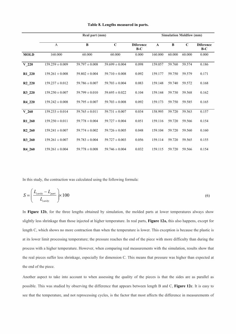
Table 8. Lengths measured in parts.
Real part (mm) Simulation Moldfow (mm)
A B C Diference B-C
A B C Diference B-C
MOLD 160.000 60.000 60.000 0.000 160.000 60.000 60.000 0.000
V_220 159.259 ± 0.009 59.797 ± 0.008 59.699 ± 0.004 0.098 159.057 59.760 59.574 0.186
R1_220 159.261 ± 0.008 59.802 ± 0.004 59.710 ± 0.008 0.092 159.177 59.750 59.579 0.171
R2_220 159.237 ± 0.012 59.786 ± 0.007 59.703 ± 0.004 0.083 159.148 59.740 59.572 0.168
R3_220 159.250 ± 0.007 59.799 ± 0.010 59.695 ± 0.022 0.104 159.144 59.730 59.568 0.162
R4_220 159.242 ± 0.008 59.795 ± 0.007 59.703 ± 0.008 0.092 159.173 59.750 59.585 0.165
V_260 159.233 ± 0.014 59.765 ± 0.011 59.731 ± 0.007 0.034 158.995 59.720 59.563 0.157
R1_260 159.250 ± 0.011 59.778 ± 0.004 59.727 ± 0.004 0.051 159.116 59.720 59.566 0.154
R2_260 159.241 ± 0.007 59.774 ± 0.002 59.726 ± 0.005 0.048 159.104 59.720 59.560 0.160
R3_260 159.261 ± 0.007 59.783 ± 0.004 59.727 ± 0.003 0.056 159.114 59.720 59.565 0.155
R4_260 159.261 ± 0.004 59.778 ± 0.008 59.746 ± 0.004 0.032 159.115 59.720 59.566 0.154
In this study, the contraction was calculated using the following formula:
100cavity part
cavity
L LS
L
(6)
In Figure 12b, for the three lengths obtained by simulation, the molded parts at lower temperatures always show
slightly less shrinkage than those injected at higher temperature. In real parts, Figure 12a, this also happens, except for
length C, which shows no more contraction than when the temperature is lower. This exception is because the plastic is
at its lower limit processing temperature; the pressure reaches the end of the piece with more difficulty than during the
process with a higher temperature. However, when comparing real measurements with the simulation, results show that
the real pieces suffer less shrinkage, especially for dimension C. This means that pressure was higher than expected at
the end of the piece.
Another aspect to take into account to when assessing the quality of the pieces is that the sides are as parallel as
possible. This was studied by observing the difference that appears between length B and C, Figure 12c. It is easy to
see that the temperature, and not reprocessing cycles, is the factor that most affects the difference in measurements of

the part. At higher temperatures there is less difference of measurements. In reality, the pieces have been obtained with
less difference in the measurements than predicted by the simulator.
It can be concluded that the contraction of the reprocessed parts does not depend on reprocessing cycles, but depends on
the injection temperature; the lower the temperature the less shrinkage. However, at higher temperatures parts are
obtained with the sides more parallel. Therefore, shrinkage dependes mainly on the maximum pressure reached in the
cavity. Shen et al. (2007) also found that at higher temperatures more shrinkage was produced and at higher pressure of
compaction less shrinkage occurred. Tang et al. (2007) measured the deformation of one piece 120·50 mm and showed
that at a lower temperature, less deformation occurred.
Other authors have obtained similar results. Chang and Faison (2001) experimented at temperatures of 218 and 252 °C
and injection pressures of 64 to 71 MPas, with parts of dimensions: 127 · 12.8 · 3.18 mm3, obtaining contractions in
both longitudinal and transversal to the flow. Chang also noted that the parts obtained in the mold (average longitudinal
shrinkage, 0.76% and transversal, 0.51%) were less than that obtained by simulation (longitudinal, 1.11% and
transversal, 0.72%).
Figure 12. Real and simulated shrinkage in the parts. Difference in width in the parts.
4.2. The influence of the addition of SEBS on the properties of degraded ABS
Modern industrial activity requires fast, efficient production processes that enhance the company’s ability to compete in
the market place. In this case, in order to transform ABS high reprocessing temperatures are necessary to adequately fill
the mold cavity. However, the use of these temperatures causes losses in ductility that dramatically limit the uses and
applications of degraded ABS. The objective of this second section is to recover this lost ductility through the addition
of SEBS to the degraded ABS and to check how the viscosity, pressure in the cavity and shrinkage of the part is
affected by the addition of SEBS to the degraded ABS. Other authors have recovered ductile properties through the
incorporation of SIS, Tasdemir (2004), or SBS, Tasdemir and Karatop (2006), but these additives possess a C=C double
bond structure which with time causes the crosslinking phenomenon to appear.
Although the variation in properties is more accentuated in the samples reprocessed at 260 ºC, in this section, the effect
of integration of SEBS with ABS at 220 ºC and 260 ºC is studied.
4.2.1. Mechanical properties
One of the principal objectives of incorporating SEBS is the recovery of impact strength, given that this is the property
that shows the greatest decrease with repeated reprocessing cycles, above all in the ABS reprocessed at 260 ºC.
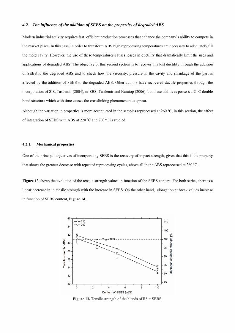
Figure 13 shows the evolution of the tensile strength values in function of the SEBS content. For both series, there is a
linear decrease in in tensile strength with the increase in SEBS. On the other hand, elongation at break values increase
in function of SEBS content, Figure 14.
Figure 13. Tensile strength of the blends of R5 + SEBS.

Figure 14. Elongation at break of the blends of R5 + SEBS.
Finally, the addition of SEBS to reprocessed ABS causes an increase in impact strength, both at 220 ºC and 260 ºC. We
saw that the evolution of the values is different, as for the ABS degraded at 260 ºC the increase in impact energy is
linear, whereas the ABS degraded at 220 ºC has an initial stage in which impact energy increases rapidly up to 5 %
SEBS content, and a second stage in which greater contents of SEBS only slightly increase this value, Figure 15.
The incorporation of SEBS and other elastic thermoplastics has been carried out by Ganguly et al. (2008), Tasdemir
(2004), Tasdemir and Karatop (2006) and Yin et al. (2007) with similar results.
Figure 15. Impact strength of the mixtures of R5 + SEBS.

4.2.2. Rheological characterization
The incorporation of additives of any polymer causes variations in the rheological behavior. In this case, the presence of
SEBS caused a reduction in viscosity in all the samples tested. Table 9 shows the values of the Cross-WLF model and
the viscosity of the material at zero shear rate at two test temperatures, 220 ºC y 260 ºC.
Table 9. Dependent parameters of the Cross-WLF model and the viscosity of the material at zero shear rate.
Material n [-] * [Pa] D1 [Pa·s] D2 [ºC] D3 [K/Pa] A1 [-] Ã2 [K] 0 [Pa/s] 0 [Pa/s]
220 ºC 260 ºC
V 0.23493 81,101 2.34·1011 378.15 0 25.9608 51.6 3855.0 812.7
R5_220_0 0.25999 68,512 1.68·1011 378.15 0 25.4620 51.6 3920.8 851.7
R5_220_2.5 0.30177 57,350 6.80·108 378.15 0 17.9979 51.6 2733.8 929.1
R5_220_5 0.29537 50,105 1.28·1011 378.15 0 25.0074 51.6 4065.4 907.5
R5_220_10 0.30309 37,978 9.70·1012 378.15 0 30.8345 51.6 5537.4 871.5
R5_260_0 0.25142 82,034 3.12·1011 378.15 0 26.6870 51.6 3114.7 628.7
R5_260_2.5 0.32680 40,695 7.10·1010 378.15 0 24.2341 51.6 3855.0 901.4
R5_260_5 0.32003 41,271 2.05·1011 378.15 0 25.6348 51.6 4240.8 911.7
R5_260_10 0.32131 34,023 3.47·1012 378.15 0 29.4056 51.6 5303.3 909.4
Once again, conversion of the viscosity has been performed (taking into account the data of the three dies of the
rheometer) in equations (2) and (3). For the adjustment the method of the χ2 (chi-square) has been used again and to
determine the goodness of fit the Pearson's chi-squared test has been performed. Table 10 shows the correlation data,
probability and Chi square. The uncertainty of the graphs shown in Figure 16 and Figure 17 is represented by the data
in Table 10.

Table 10. Correlation data, probability and Chi square.
Material Correlation Probability (%) χ 2 χ t2 (r-1)(k-1)
V 0.99944 100 6.628 56.942
R5_220_0 0.99838 99.99 15.067 56.942
R5_220_2.5 0.99555 86.50 31.232 56.942
R5_220_5 0.99110 14.22 50.712 56.942
R5_220_10 0.99618 97.034 25.700 56.942
R5_260_0 0.99873 99.99 13.244 56.942
R5_260_2.5 0.99615 97.42 25.296 56.942
R5_260_5 0.99278 38.456 43.025 56.942
R5_260_10 0.99599 96.680 26.032 56.942
Looking at Table 9, it is worth highlighting that the variation in the value of n increases as the percentage of
incorporation of SEBS is increased. This is more pronounced for the material reprocessed at 260 °C than for the
material reprocessed at 220 °C. This increase of n causes a slight decline in the slope. This decline in the slope of the
curve represents a slight increase in viscosity under the same conditions of zero shear rate.
The incorporation of different percentages of SEBS to the two sets of degraded materials causes the value of τ* to
disminish significantly as the percentage of SEBS increases. This behavior causes the viscosity curve to move to the left
for all the blends, representing a slight reduction in viscosity. For material reprocessed at 220 °C the decreased τ* is
flat, causing the displacement to the left be progresive depending on the increase of the quantity of SEBS. This behavior
can be observed in the Figure 16a, which shows how the viscosoty curves (characterized at 220 ºC) run side by side. For
material processed at 260 °C (220 °C characterized) (Figure 16b) the decreased * is more abrupt, causing the
separation of the two groups of curves. The first group is the curves of V and R5_260 and the second group are the
curves with various percentage of SEBS, which are all below the previous two. This behavior is best seen in Figure
17a, which shows these two levels of viscosity on the curve with R5_260 material characterized at 220 °C. Figure 16b
also shows that the amount of SEBS has more influence on the viscosity when the material is processed at high
temperature than that which has been treated at low temperature.
The variation in the value of η0, can be seen in Table 9. Again, the change in value of η0, was calculated using the
Williams-Landel-Ferry equation (3) and with shear rate data from the rheometer. We reiterate that the lower viscosity
real data obtained with the rheometer from 100 s-1 to zero shear rate was done by approximation with the equation, and
so are not very relevant.
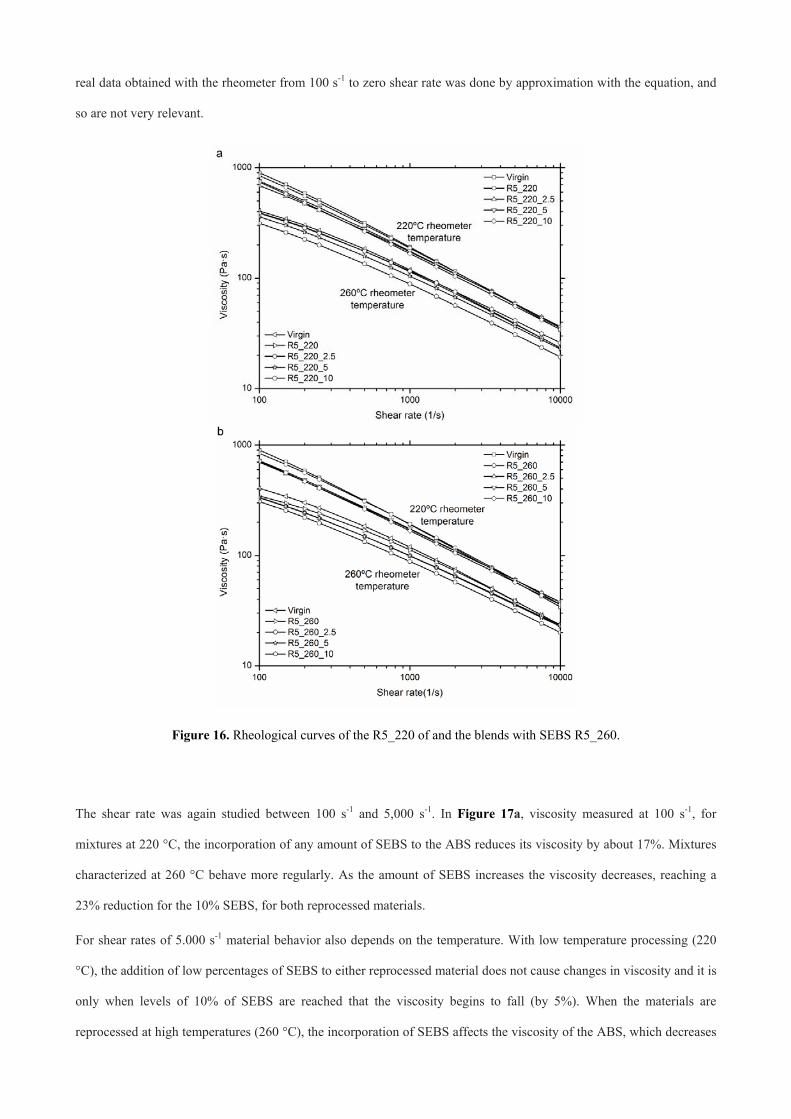
Figure 16. Rheological curves of the R5_220 of and the blends with SEBS R5_260.
The shear rate was again studied between 100 s-1 and 5,000 s-1. In Figure 17a, viscosity measured at 100 s-1, for
mixtures at 220 °C, the incorporation of any amount of SEBS to the ABS reduces its viscosity by about 17%. Mixtures
characterized at 260 °C behave more regularly. As the amount of SEBS increases the viscosity decreases, reaching a
23% reduction for the 10% SEBS, for both reprocessed materials.
For shear rates of 5.000 s-1 material behavior also depends on the temperature. With low temperature processing (220
°C), the addition of low percentages of SEBS to either reprocessed material does not cause changes in viscosity and it is
only when levels of 10% of SEBS are reached that the viscosity begins to fall (by 5%). When the materials are
reprocessed at high temperatures (260 °C), the incorporation of SEBS affects the viscosity of the ABS, which decreases

progressively and linearly as the percentage of SEBS is increased, with the addition of 10% of SEBS causing a 20%
reduction in viscosity, see Figure 17b.
Figure 17. Viscosity of the mixtures at 100 s-1 and 5,000 s-1.
Other authors have obtained similar results. For example, the same results were obtained by Tasdemir ( 2004) and
Tasdemir and Karatop (2006) , who also saw a reduction in viscosity. He used styrene-butadiene-styrene (SBS) and
styrene-isopren-styrene (SIS) as compatibilizers in blends of ABS / PC. The SBS and SIS materials are very similar to
SEBS. The drop in viscosity is due to the low viscosity of the SEBS, which allows the fluidization of the mixture
generated.

4.2.3. Analysis of the pressures in the mold.
The drop in viscosity of the mixtures of ABS reprocessed with different percentages of SEBS, is also reflected in the
drop in pressure in the mold cavity. Table 11 shows how the maximum pressure reached in the filling decreases with
increasing percentages of SEBS.
Besides the pressure drop necessary to inject the parts, the incorporation of SEBS, has caused the aforementioned
decrease in viscosity, which in turn has caused the occurrence of flash. To avoid this defect the injection rate was as the
amount of SEBS was increased. This effect can be seen perfectly in the graphs in Figure 18. The figure shows how the
data obtained in the mold cavity are similar to those predicted by the simulation.
The pressures listed in Table 11 are obtained from the hydraulic circuit of the injection machine. These data are
interesting because, although one can not directly compare with the pressure values in the mold, the variation of these
values reflects the variation in pressure in the mold. For comparison it is important to take into account that the
compression ratio between the barrel of the injection machine and the oil circuit is 10/1 and that the injection machine
has a pressure loss. Thus, the table values expressed in bars are comparable to those obtained in the mold in MPas.
Thus, for the temperature of 220 °C, varying the pressure of the hydraulic circuit in the packing phase (Packing
pressure in Table 11) between the virgin material and the mixture with 10% SEBS goes from 96 to 85 bar (down 11,
4%), and the pressure drop point P1 in the mold (Figure 18b) moves from 66 to 59 MPas, showing a decrease of
10.6%, very similar to the hydraulic circuit.
Table 11. Parameters introduced and obtained from the injection machine.
Injection temperature (ºC) 220 ºC 260 ºC
Material V R5_2.5 R5_5 R5_10 V R5_2.5 R5_2.5 R5_2.5
Injection time (s) 1.3 1.3 1.3 1.3 0.8 0.8 0.8 0.8
Packing time (s) 10 10 10 10 12 12 12 12
Mold closed time (s) 5 5 5 5 5 5 5 5
Filling, 100 % (dmm) 340 340 340 340 300 300 300 300
Filling, swich-over 95 % (dmm) 323 323 323 323 285 285 285 285
Injection shot (dmm) 200 200 200 200 200 200 200 200
Suction distance (dmm) 0 0 0 0 0 0 0 0
Shot distance (dmm) 523 523 523 523 485 485 485 485
Injection rate (%) 22 22 22 22 35 35 35 35

Maximum injection pressure (bar)
120 118 115 110 95 95 90 90
Packing pressure; percentage over maximum injection pressure (%)
80 80 80 75 70 70 65 60
Packing pressure (bar) 96 94 92 85 66 66 60 55
Shutoff nozzle (offset) 1,610 1,610 1,610 1,610 1,610 1,610 1,610 1,610
Mold temperature (ºC) 50 50 50 50 50 50 50 50
Clamp force; in simulation (tons) 52.95 59.05 53.29 42.77 41.59 41.26 34.56 27.05
Figure 18. Graphic "Pressure - Cycle time" in Moldflow and mold for 220 °C and 260 °C in ABS with SEBS.
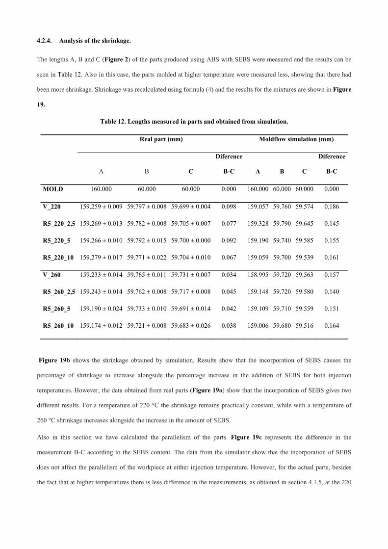
4.2.4. Analysis of the shrinkage.
The lengths A, B and C (Figure 2) of the parts produced using ABS with SEBS were measured and the results can be
seen in Table 12. Also in this case, the parts molded at higher temperature were measured less, showing that there had
been more shrinkage. Shrinkage was recalculated using formula (4) and the results for the mixtures are shown in Figure
19.
Table 12. Lengths measured in parts and obtained from simulation.
Real part (mm) Moldflow simulation (mm)
A B C
Diference
B-C A B C
Diference
B-C
MOLD 160.000 60.000 60.000 0.000 160.000 60.000 60.000 0.000
V_220 159.259 ± 0.009 59.797 ± 0.008 59.699 ± 0.004 0.098 159.057 59.760 59.574 0.186
R5_220_2,5 159.269 ± 0.013 59.782 ± 0.008 59.705 ± 0.007 0.077 159.328 59.790 59.645 0.145
R5_220_5 159.266 ± 0.010 59.792 ± 0.015 59.700 ± 0.000 0.092 159.190 59.740 59.585 0.155
R5_220_10 159.279 ± 0.017 59.771 ± 0.022 59.704 ± 0.010 0.067 159.059 59.700 59.539 0.161
V_260 159.233 ± 0.014 59.765 ± 0.011 59.731 ± 0.007 0.034 158.995 59.720 59.563 0.157
R5_260_2,5 159.243 ± 0.014 59.762 ± 0.008 59.717 ± 0.008 0.045 159.148 59.720 59.580 0.140
R5_260_5 159.190 ± 0.024 59.733 ± 0.010 59.691 ± 0.014 0.042 159.109 59.710 59.559 0.151
R5_260_10 159.174 ± 0.012 59.721 ± 0.008 59.683 ± 0.026 0.038 159.006 59.680 59.516 0.164
Figure 19b shows the shrinkage obtained by simulation. Results show that the incorporation of SEBS causes the
percentage of shrinkage to increase alongside the percentage increase in the addition of SEBS for both injection
temperatures. However, the data obtained from real parts (Figure 19a) show that the incorporation of SEBS gives two
different results. For a temperature of 220 °C the shrinkage remains practically constant, while with a temperature of
260 °C shrinkage increases alongside the increase in the amount of SEBS.
Also in this section we have calculated the parallelism of the parts. Figure 19c represents the difference in the
measurement B-C according to the SEBS content. The data from the simulator show that the incorporation of SEBS
does not affect the parallelism of the workpiece at either injection temperature. However, for the actual parts, besides
the fact that at higher temperatures there is less difference in the measurements, as obtained in section 4.1.5, at the 220

°C temperature the difference in the measurements decreases with the increase in the percentage of SEBS. On the other
hand, for the temperature of 260 °C this difference increases with the presence of SEBS.
Figure 19. Real and simulated shrinkage in the parts. Difference in the width of the parts with SEBS.
5. CONCLUSIONS
The possibility of processing polymers at a range of temperatures has created the need for studies into the effect of
temperature when the polymer is reprocessed. In this case, ABS reprocessed at the limit temperatures (220 ºC and 260
ºC) shows significant differences in the evolution of its properties.
The properties (mechanical and rheological) of ABS reprocessed at 220 ºC remain virtually unchanged with the number
of cycles. On the other hand, when the ABS is reprocessed 260 ºC, variations in both the mechanical and rheological
properties are seen. Of these variations, it is particularly worth highlighting the considerable loss of ductility in the
ABS. This takes place due to the crosslinking effect of the ABS. This phenomenon can be easily observed using DSC.
A decrease in the enthalpy of the crosslinking as the number of cycles increased was observed, and this decrease was
more noticeable in the samples reprocessed at 260 ºC than those reprocessed at 220 ºC.
Moreover, the crosslinking effect should increase the viscosity of the material. Although the total number of crosslinks
increases with the number of processes, the quantity of the butadiene phase within the polymer is so small that the
degradation effect due to temperature and shear stress (breaks in the polymer chain) is greater than the crosslinking, and
thus the viscosity of the reprocessed material is slightly lower than the virgin ABS.
In relation to the pressure in the cavity, at a higher temperature less pressure is required to fill the cavity. To be more
precise, with a difference of 40 °C in temperature, there is a 30% drop in pressure.

Concerning the shrinkage of the part, at lower temperatures less shrinkage is obtained, however, at higher temperature
parts are obtained with sides that are more parallel.
With the aim of recovering the ductility of degraded ABS, this material was mixed with SEBS. The presence of SEBS
in the degraded ABS allowed the recovery of the lost ductility, but in turn a decrease in the tensile strength values was
seen. The material reprocessed at 220 ºC would not need to be mixed with SEBS. On the other hand, the material
reprocessed at 260 ºC would have to be mixed with at least 5 % SEBS. This mixture would recover up to 75 % of the
impact energy. Mixtures with larger proportions of SEBS would produce an excessive reduction in tensile strength.
In terms of rheological properties, the SEBS reduces viscosity, which allows reduction of the temperature and injection
time during transformation. This allows the producer to increase production and reduce energy consumption.
In relation to the pressure in the cavity, the drop in viscosity of the blends caused a decrease in the pressure required to
inject the parts. This is beneficial because less power is needed in the injection machine to fill the parts. But the
decrease in viscosity also causes flash if the same packing pressure is maintained. To remedy injection problems, the
packing pressure is further reduced.
Concerning shrinkage, results showed that higher temperatures cause slightly more shrinkage. However, with the
incorporation of SEBS two differing results were produced. At a temperature of 220 °C shrinkage remained practically
constant, while at the temperature of 260 °C it increased with the increase in the amount of SEBS.
In this work we concluded that the quantity of 5% SEBS, for the reprocessed material at 260 °C, is the ideal amount that
recovers a large part of the material’s mechanical properties.
ACKNOWLEDGEMENTS
We would like to thank the Vice-Directorate of Research, Development and Innovation of the Polytechnic University of
Valencia for the help granted to the project: “Ternary systems research applied to polymeric materials for the upgrading
of waste styrene”, Ref: 20091056 within the program of First Projects of Investigation (PAID 06-09) where this work is
framed.

6. REFERENCES
Bai, X.J., Isaac, D.H., Smith, K., 2007. Reprocessing acrylonitrile-butadiene-styrene plastics: Structure-property relationships. Polymer Engineering and Science 47, 120-130.
Balart, R., Lopez, J., Garcia, D., Salvador, M.D., 2005. Recycling of ABS and PC from electrical and electronic waste. Effect of miscibility and previous degradation on final performance of industrial blends. European Polymer Journal 41, 2150-2160.
Boronat, T., Segui, V.J., Peydro, M.A., Reig, M.J., 2009. Influence of temperature and shear rate on the rheology and processability of reprocessed ABS in injection molding process. Journal of Materials Processing Technology 209, 2735-2745.
Cross, M.M., 1965. Rheology of Non-Newtonian Fluids - a New Flow Equation for Pseudoplastic Systems. Journal of Colloid Science 20, 417-437.
Chang, T.C., Faison, E., 2001. Shrinkage behavior and optimization of injection molded parts studied by the Taguchi method. Polym. Eng. Sci. 41, 703-710.
Eguiazabal, J.I., Nazabal, J., 1990. Reprocessing polycarbonate Acrylonitrile-Butadiene-Styrene blends - influence on physical-properties. Polymer Engineering and Science 30, 527-531.
Flores, A., Pieruccini, M., Nochel, U., Stribeck, N., Calleja, F.J.B., 2008. Recrystallization studies on isotropic cold-crystallized PET: Influence of heating rate. Polymer 49, 965-973.
Ganguly, A., Saha, S., Bhowmick, A.K., Chattopadhyay, S., 2008. Augmenting the performance of acrylonitrile-butadiene-styrene plastics for low-noise dynamic applications. Journal of Applied Polymer Science 109, 1467-1475.
Karahaliou, E.K., Tarantili, P.A., 2009. Stability of ABS Compounds Subjected to Repeated Cycles of Extrusion Processing. Polymer Engineering and Science 49, 2269-2275.
Li, B., Wan, C.Y., Zhang, Y., Ji, J.L., 2010. Blends of Poly(2,6-dimethyl-1,4-phenylene oxide)/Polyamide 6 Toughened by Maleated Polystyrene-based Copolymers: Mechanical Properties, Morphology, and Rheology. Journal of Applied Polymer Science 115, 3385-3392.
Liu, X.D., Boldizar, A., Rigdahl, M., Bertilsson, H., 2002. Recycling of blends of acrylonitrile-butadiene-styrene (ABS) and polyamide. Journal of Applied Polymer Science 86, 2535-2543.
Navarro, R., Ferrandiz, S., Lopez, J., Segui, V.J., 2008. The influence of polyethylene in the mechanical recycling of polyethylene terephtalate. Journal of Materials Processing Technology 195, 110-116.
Ozcelik, B., Sonat, I., 2009. Warpage and structural analysis of thin shell plastic in the plastic injection molding. Mater. Des. 30, 367-375.
Perez, J.M., Vilas, J.L., Laza, J.M., Arnaiz, S., Mijangos, F., Bilbao, E., Leon, L.M., 2010. Effect of Reprocessing and Accelerated Weathering on ABS Properties. Journal of Polymers and the Environment 18, 71-78.
Peydro, M.A., Parres, F., Crespo, J.E., Juarez, D., 2011. Study of Rheological Behavior During the Recovery Process of High Impact Polystyrene Using Cross-WLF Model. Journal of Applied Polymer Science 120, 2400-2410.
Reig, M.J., Segui, V.J., Ferrandiz, S., Zamanillo, J.D., 2007. An evaluation of processability by injection molding of ABS/PC blends obtained from recycled materials. Journal of Polymer Engineering 27, 29-54.
Reig, M.J., Segui, V.J., Zamanillo, J.D., 2005. Rheological behavior modeling of recycled ABS/PC blends applied to injection molding process. Journal of Polymer Engineering 25, 435-457.
Salari, D., Ranjbar, H., 2008. Study on the recycling of ABS resins: Simulation of reprocessing and thermo-oxidation. Iranian Polymer Journal 17, 599-610.
Shen, C.Y., Wang, L.X., Li, Q., 2007. Optimization of injection molding process parameters using combination of artificial neural network and genetic algorithm method. Journal of Materials Processing Technology 183, 412-418.
Shin, H., Park, E.S., 2009. Analysis of Crack Phenomenon for Injection-Molded Screw Using Moldflow Simulation. Journal of Applied Polymer Science 113, 2702-2708.
Tang, S.H., Tan, Y.J., Sapuan, S.M., Sulaiman, S., Ismail, N., Samin, R., 2007. The use of Taguchi method in the design of plastic injection mould for reducing warpage. Journal of Materials Processing Technology 182, 418-426.
Tasdemir, M., 2004. Properties of acrylonitrile-butadiene-styrene/polycarbonate blends with styrene-butadiene-styrene block copolymer. Journal of Applied Polymer Science 93, 2521-2527.
Tasdemir, M., Karatop, S., 2006. Effect of styrene-isopren-styrene addition on the recycled polycarbonate/acrylonitrile-butadiene-styrene polymer blends. Journal of Applied Polymer Science 101, 559-566.
Williams, M.L., Landel, R.F., Ferry, J.D., 1955. Mechanical Properties of Substances of High Molecular Weight .19. the Temperature Dependence of Relaxation Mechanisms in Amorphous Polymers and Other Glass-Forming Liquids. Journal of the American Chemical Society 77, 3701-3707.
Yin, N.A.W., Zhang, Y.X., Zhang, Y., Zhang, X.F., Zhou, W., 2007. Preparation and properties of PC/SAN alloy modified with styrene-ethylene-butylene-styrene block copolymer. Journal of Applied Polymer Science 106, 637-643.

Table Caption
Table 1. Mechanical characterization values of the virgin ABS and virgin SEBS.
Table 2. Samples code.
Table 3. Results of the simulation process.
Table 4. Injection molding cycle.
Table 5. Mechanical characterization values of the reprocessed ABS at 220 ºC and 260 ºC.
Table 6. Correlation data, probability and Chi square.
Table 7. Dependent parameters of the Cross-WLF model.
Table 8. Lengths measured in parts.
Table 9. Dependent parameters of the Cross-WLF model and the viscosity of the material at zero shear rate.
Table 10. Correlation data, probability and Chi square.
Table 11. Parameters introduced and obtained from the injection machine.
Table 12. Lengths measured in parts and obtained from simulation.
Figure Caption
Figure 1. Rheological curves virgin ABS at 220 ºC and 260 ºC and virgin SEBS at 180 ºC and 200 ºC.
Figure 2. Geometry of injected part and position of pressure and temperature sensors.
Figure 3. Viscosity of virgin material at 200, 220, 240, 260 and 280 ºC.
Figure 4. Calorimetric curve of virgin ABS and R5. Cp of sapphire, virgin ABS and R5.
Figure 5. Pressures obtained in the simulator by injecting at 220 °C with virgin material.
Figure 6. Temperatures in part and sprue versus cycle time for virgin material injected at 220 °C.
Figure 7. Values of Tg in function of processing cycles at 220 ºC and 260 ºC.
Figure 8. Crosslinking enthalpy in function of reprocessing cycles at 220 ºC and 260 ºC.
Figure 9. Viscosity of virgin and reprocessed material at 220 ºC and 260 ºC.
Figure 10.Viscosity of virgin and reprocessed material at shear rate of 100 and 5,000 s-1.
Figure 11. Graphic "Pressure - Cycle time" in Moldflow and mold, for temperatures of 220 °C and 260 °C.
Figure 12. Real and simulated shrinkage in the parts. Difference in width in the parts.
Figure 13. Tensile strength of the blends of R5 + SEBS.
Figure 14. Elongation at break of the blends of R5 + SEBS.
Figure 15. Impact strength of the mixtures of R5 + SEBS.
Figure 16. Rheological curves of the R5_220 of and the blends with SEBS R5_260.

Figure 17. Viscosity of the mixtures at 100 s-1 and 5,000 s-1.
Figure 18. Graphic "Pressure - Cycle time" in Moldflow and mold for 220 °C and 260 °C in ABS with SEBS.
Figure 19. Real and simulated shrinkage in the parts. Difference in the width of the parts with SEBS.