Phenomenology of Particle Physics

NIU Fall 2018 PHYS 686 Lecture Notes

Stephen P. Martin

Physics DepartmentNorthern Illinois University

DeKalb IL 60115spmartin@niu.edu

August 22, 2018

1

Contents

1 Introduction 41.1 Fundamental forces . . . . . . . . . . . . . . . . . . . . . . . . . . . . . . . . . . . . . . . 41.2 Resonances, widths, and lifetimes . . . . . . . . . . . . . . . . . . . . . . . . . . . . . . . 51.3 Leptons and quarks . . . . . . . . . . . . . . . . . . . . . . . . . . . . . . . . . . . . . . . 61.4 Hadrons . . . . . . . . . . . . . . . . . . . . . . . . . . . . . . . . . . . . . . . . . . . . . 71.5 Decays and branching ratios . . . . . . . . . . . . . . . . . . . . . . . . . . . . . . . . . . 12

2 Special Relativity and Lorentz Transformations 152.1 Lorentz transformations . . . . . . . . . . . . . . . . . . . . . . . . . . . . . . . . . . . . 152.2 Relativistic kinematics . . . . . . . . . . . . . . . . . . . . . . . . . . . . . . . . . . . . . 182.3 Tensors and Lorentz invariant quantities . . . . . . . . . . . . . . . . . . . . . . . . . . . 222.4 Maxwell’s equations and electromagnetism . . . . . . . . . . . . . . . . . . . . . . . . . . 25

3 Relativistic Quantum Mechanics of Single Particles 283.1 Klein-Gordon and Dirac equations . . . . . . . . . . . . . . . . . . . . . . . . . . . . . . 283.2 Solutions of the Dirac equation . . . . . . . . . . . . . . . . . . . . . . . . . . . . . . . . 353.3 The Weyl equation . . . . . . . . . . . . . . . . . . . . . . . . . . . . . . . . . . . . . . . 433.4 Majorana fermions . . . . . . . . . . . . . . . . . . . . . . . . . . . . . . . . . . . . . . . 45

4 Field Theory and Lagrangians 464.1 The field concept and Lagrangian dynamics . . . . . . . . . . . . . . . . . . . . . . . . . 464.2 Quantization of free scalar field theory . . . . . . . . . . . . . . . . . . . . . . . . . . . . 534.3 Quantization of free Dirac fermion field theory . . . . . . . . . . . . . . . . . . . . . . . 584.4 Scalar field with φ4 coupling . . . . . . . . . . . . . . . . . . . . . . . . . . . . . . . . . . 614.5 Scattering processes and cross-sections . . . . . . . . . . . . . . . . . . . . . . . . . . . . 674.6 Scalar field with φ3 coupling . . . . . . . . . . . . . . . . . . . . . . . . . . . . . . . . . . 774.7 Feynman rules . . . . . . . . . . . . . . . . . . . . . . . . . . . . . . . . . . . . . . . . . 84

5 Quantum Electro-Dynamics (QED) 925.1 QED Lagrangian and Feynman rules . . . . . . . . . . . . . . . . . . . . . . . . . . . . . 925.2 Electron-positron scattering . . . . . . . . . . . . . . . . . . . . . . . . . . . . . . . . . . 100

5.2.1 e−e+ → µ−µ+ . . . . . . . . . . . . . . . . . . . . . . . . . . . . . . . . . . . . . 1005.2.2 e−e+ → ff . . . . . . . . . . . . . . . . . . . . . . . . . . . . . . . . . . . . . . . . 1055.2.3 Helicities in e−e+ → µ−µ+ . . . . . . . . . . . . . . . . . . . . . . . . . . . . . . 1105.2.4 Bhabha scattering (e−e+ → e−e+) . . . . . . . . . . . . . . . . . . . . . . . . . . 118

5.3 Crossing symmetry . . . . . . . . . . . . . . . . . . . . . . . . . . . . . . . . . . . . . . . 1235.3.1 e−µ+ → e−µ+ and e−µ− → e−µ− . . . . . . . . . . . . . . . . . . . . . . . . . . 1245.3.2 Møller scattering (e−e− → e−e−) . . . . . . . . . . . . . . . . . . . . . . . . . . . 126

5.4 Gauge invariance in Feynman diagrams . . . . . . . . . . . . . . . . . . . . . . . . . . . 1285.5 External photon scattering . . . . . . . . . . . . . . . . . . . . . . . . . . . . . . . . . . 130

5.5.1 Compton scattering (γe− → γe−) . . . . . . . . . . . . . . . . . . . . . . . . . . . 1305.5.2 e+e− → γγ . . . . . . . . . . . . . . . . . . . . . . . . . . . . . . . . . . . . . . . 138

6 Decay Processes 1406.1 Decay rates and partial widths . . . . . . . . . . . . . . . . . . . . . . . . . . . . . . . . 1406.2 Two-body decays . . . . . . . . . . . . . . . . . . . . . . . . . . . . . . . . . . . . . . . . 1416.3 Scalar decays to fermion-antifermion pairs: Higgs decay . . . . . . . . . . . . . . . . . . 1436.4 Three-body decays . . . . . . . . . . . . . . . . . . . . . . . . . . . . . . . . . . . . . . . 147

2

7 Fermi Theory of Weak Interactions 1507.1 Weak nuclear decays . . . . . . . . . . . . . . . . . . . . . . . . . . . . . . . . . . . . . . 1507.2 Muon decay . . . . . . . . . . . . . . . . . . . . . . . . . . . . . . . . . . . . . . . . . . . 1527.3 Corrections to muon decay . . . . . . . . . . . . . . . . . . . . . . . . . . . . . . . . . . 1627.4 Inverse muon decay (e−νµ → νeµ

−) . . . . . . . . . . . . . . . . . . . . . . . . . . . . . . 1647.5 e−νe → µ−νµ . . . . . . . . . . . . . . . . . . . . . . . . . . . . . . . . . . . . . . . . . . 1677.6 Charged currents and π± decay . . . . . . . . . . . . . . . . . . . . . . . . . . . . . . . . 1687.7 Unitarity, renormalizability, and the W boson . . . . . . . . . . . . . . . . . . . . . . . . 175

8 Gauge theories 1808.1 Groups and representations . . . . . . . . . . . . . . . . . . . . . . . . . . . . . . . . . . 1808.2 The Yang-Mills Lagrangian and Feynman rules . . . . . . . . . . . . . . . . . . . . . . . 191

9 Quantum Chromo-Dynamics (QCD) 1989.1 QCD Lagrangian and Feynman rules . . . . . . . . . . . . . . . . . . . . . . . . . . . . . 1989.2 Scattering of quarks and gluons . . . . . . . . . . . . . . . . . . . . . . . . . . . . . . . . 200

9.2.1 Quark-quark scattering (qq → qq) . . . . . . . . . . . . . . . . . . . . . . . . . . 2009.2.2 Gluon-gluon scattering (gg → gg) . . . . . . . . . . . . . . . . . . . . . . . . . . . 203

9.3 Renormalization . . . . . . . . . . . . . . . . . . . . . . . . . . . . . . . . . . . . . . . . 2049.4 Parton distribution functions and hadron-hadron scattering . . . . . . . . . . . . . . . . 2159.5 Top-antitop production in pp and pp collisions . . . . . . . . . . . . . . . . . . . . . . . . 2249.6 Kinematics in hadron-hadron scattering . . . . . . . . . . . . . . . . . . . . . . . . . . . 2289.7 Drell-Yan scattering (ℓ+ℓ− production in hadron collisions) . . . . . . . . . . . . . . . . 231

10 Spontaneous Symmetry Breaking 23510.1 Global symmetry breaking . . . . . . . . . . . . . . . . . . . . . . . . . . . . . . . . . . . 23510.2 Local symmetry breaking and the Higgs mechanism . . . . . . . . . . . . . . . . . . . . 23910.3 Goldstone’s Theorem and the Higgs mechanism in general . . . . . . . . . . . . . . . . . 242

11 The Standard Electroweak Model 24511.1 SU(2)L × U(1)Y representations and Lagrangian . . . . . . . . . . . . . . . . . . . . . . 24511.2 The Standard Model Higgs mechanism . . . . . . . . . . . . . . . . . . . . . . . . . . . . 25011.3 Fermion masses and Cabibbo-Kobayashi-Maskawa mixing . . . . . . . . . . . . . . . . . 25511.4 Neutrino masses and the seesaw mechanism . . . . . . . . . . . . . . . . . . . . . . . . . 26411.5 The Higgs boson discovery . . . . . . . . . . . . . . . . . . . . . . . . . . . . . . . . . . . 266

11.5.1 Higgs boson decays revisited . . . . . . . . . . . . . . . . . . . . . . . . . . . . . 26711.5.2 Higgs boson production at the LHC . . . . . . . . . . . . . . . . . . . . . . . . . 27111.5.3 The Higgs boson discovery . . . . . . . . . . . . . . . . . . . . . . . . . . . . . . 275

Further Reading 278

Appendices 279A.1 Natural units and conversions . . . . . . . . . . . . . . . . . . . . . . . . . . . . . . . . . 279A.2 Dirac Spinor Formulas . . . . . . . . . . . . . . . . . . . . . . . . . . . . . . . . . . . . . 280

Index 281

3

1 Introduction

In this course, we will explore some of the tools necessary for attacking the fundamental questions

of elementary particle physics. These questions include:

• What fundamental particles is everything made out of?

• How do the particles interact with each other?

• What principles underlie the answers to these questions?

• How can we use this information to predict and interpret the results of experiments?

The Standard Model of particle physics proposes some answers to these questions. Although

it is highly doubtful that the Standard Model will survive intact beyond this decade, it is the

benchmark against which future theories will be compared. Furthermore, it is highly likely that

the new physics to be uncovered at the CERN Large Hadron Collider (LHC) can be described

using the same set of tools.

This Introduction contains a brief outline of the known fundamental particle content of the

Standard Model, for purposes of orientation. These and many other experimental results about

elementary particles can be found in the Review of Particle Properties, hereafter known as the

RPP, authored by the Particle Data Group, and in its pocket-sized abridged form, the Particle

Physics Booklet. The current edition of the RPP was published as M. Tanabashi et al. (Particle

Data Group), Phys. Rev. D 98, 030001 (2018). It is updated and republished every even-

numbered year. An always-up-to-date version is available on-line, at http://pdg.lbl.gov, and

it is usually considered the definitive source for elementary particle physics data and analysis.

Each result is referenced according to the experiments that provided it. Background theoretical

material needed for interpreting the results is also included. Copies can be ordered for free from

their website.

1.1 Fundamental forces

The known interaction forces in nature are the universal attraction of gravity, the electromag-

netic force, the weak nuclear force, and the strong nuclear force. Among these, gravity is special

and is governed by Einstein’s theory of General Relativity. The other forces are gauge theories.

The definition of gauge theories and their properties will be explored extensively throughout

this book. Here let it suffice to say that a gauge force is one that is mediated by a spin-1 (vector)

boson. The force-mediator gauge bosons that we know about in the Standard Model are listed

in Table 1.1.

4

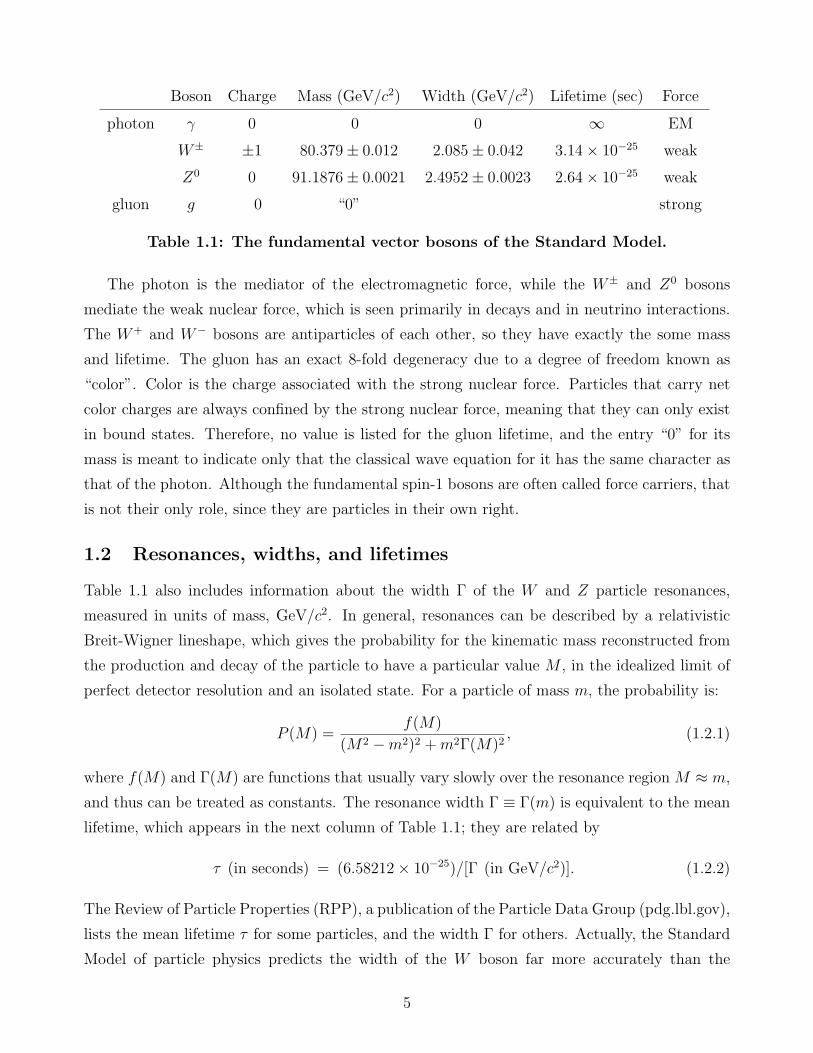
Boson Charge Mass (GeV/c2) Width (GeV/c2) Lifetime (sec) Force

photon γ 0 0 0 ∞ EM

W± ±1 80.379± 0.012 2.085± 0.042 3.14× 10−25 weak

Z0 0 91.1876± 0.0021 2.4952± 0.0023 2.64× 10−25 weak

gluon g 0 “0” strong

Table 1.1: The fundamental vector bosons of the Standard Model.

The photon is the mediator of the electromagnetic force, while the W± and Z0 bosons

mediate the weak nuclear force, which is seen primarily in decays and in neutrino interactions.

The W+ and W− bosons are antiparticles of each other, so they have exactly the some mass

and lifetime. The gluon has an exact 8-fold degeneracy due to a degree of freedom known as

“color”. Color is the charge associated with the strong nuclear force. Particles that carry net

color charges are always confined by the strong nuclear force, meaning that they can only exist

in bound states. Therefore, no value is listed for the gluon lifetime, and the entry “0” for its

mass is meant to indicate only that the classical wave equation for it has the same character as

that of the photon. Although the fundamental spin-1 bosons are often called force carriers, that

is not their only role, since they are particles in their own right.

1.2 Resonances, widths, and lifetimes

Table 1.1 also includes information about the width Γ of the W and Z particle resonances,

measured in units of mass, GeV/c2. In general, resonances can be described by a relativistic

Breit-Wigner lineshape, which gives the probability for the kinematic mass reconstructed from

the production and decay of the particle to have a particular value M , in the idealized limit of

perfect detector resolution and an isolated state. For a particle of mass m, the probability is:

P (M) =f(M)

(M2 −m2)2 +m2Γ(M)2, (1.2.1)

where f(M) and Γ(M) are functions that usually vary slowly over the resonance regionM ≈ m,

and thus can be treated as constants. The resonance width Γ ≡ Γ(m) is equivalent to the mean

lifetime, which appears in the next column of Table 1.1; they are related by

τ (in seconds) = (6.58212× 10−25)/[Γ (in GeV/c2)]. (1.2.2)

The Review of Particle Properties (RPP), a publication of the Particle Data Group (pdg.lbl.gov),

lists the mean lifetime τ for some particles, and the width Γ for others. Actually, the Standard

Model of particle physics predicts the width of the W boson far more accurately than the

5

experimentally measured width indicated in Table 1.1. The predicted width, with uncertainties

from input parameters, is ΓW = 2.091± 0.002 GeV/c2.

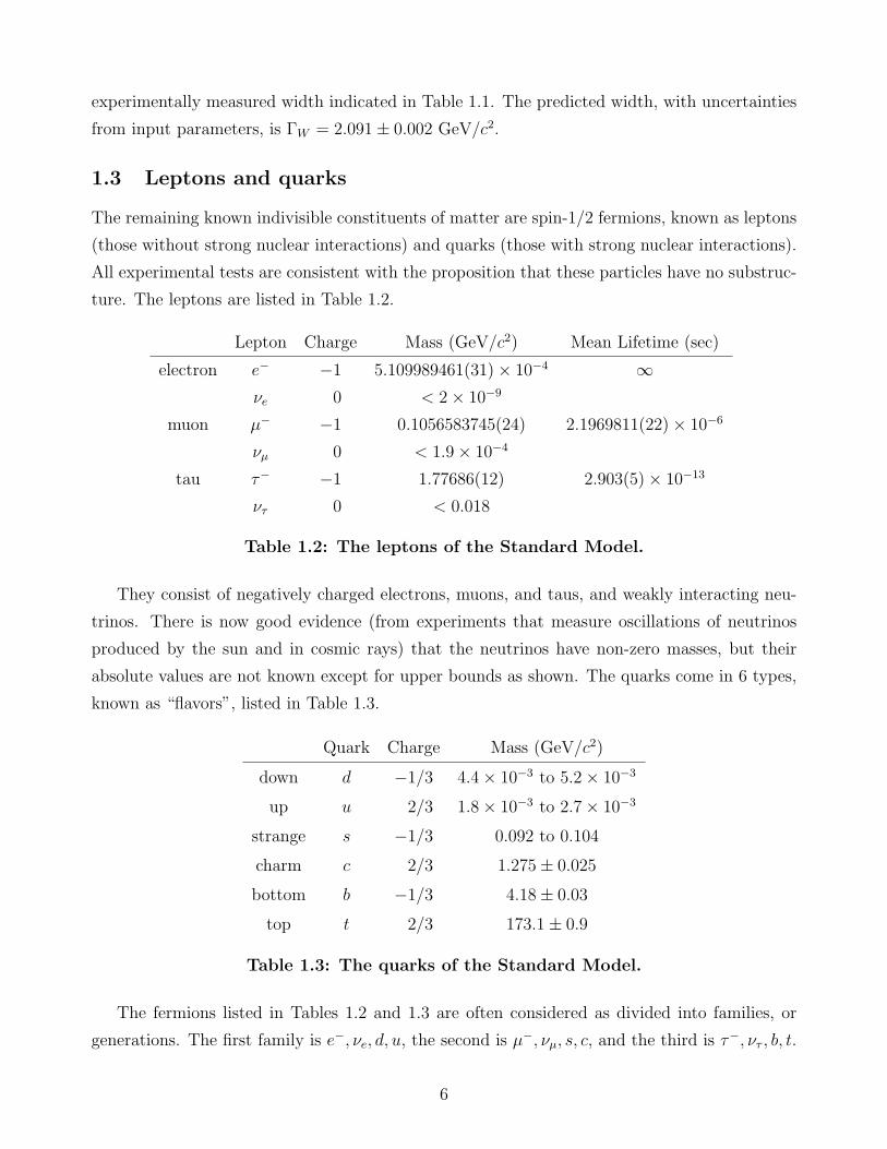
1.3 Leptons and quarks

The remaining known indivisible constituents of matter are spin-1/2 fermions, known as leptons

(those without strong nuclear interactions) and quarks (those with strong nuclear interactions).

All experimental tests are consistent with the proposition that these particles have no substruc-

ture. The leptons are listed in Table 1.2.

Lepton Charge Mass (GeV/c2) Mean Lifetime (sec)

electron e− −1 5.109989461(31)× 10−4 ∞νe 0 < 2× 10−9

muon µ− −1 0.1056583745(24) 2.1969811(22)× 10−6

νµ 0 < 1.9× 10−4

tau τ− −1 1.77686(12) 2.903(5)× 10−13

ντ 0 < 0.018

Table 1.2: The leptons of the Standard Model.

They consist of negatively charged electrons, muons, and taus, and weakly interacting neu-

trinos. There is now good evidence (from experiments that measure oscillations of neutrinos

produced by the sun and in cosmic rays) that the neutrinos have non-zero masses, but their

absolute values are not known except for upper bounds as shown. The quarks come in 6 types,

known as “flavors”, listed in Table 1.3.

Quark Charge Mass (GeV/c2)

down d −1/3 4.4× 10−3 to 5.2× 10−3

up u 2/3 1.8× 10−3 to 2.7× 10−3

strange s −1/3 0.092 to 0.104

charm c 2/3 1.275± 0.025

bottom b −1/3 4.18± 0.03

top t 2/3 173.1± 0.9

Table 1.3: The quarks of the Standard Model.

The fermions listed in Tables 1.2 and 1.3 are often considered as divided into families, or

generations. The first family is e−, νe, d, u, the second is µ−, νµ, s, c, and the third is τ−, ντ , b, t.

6

The masses of the fermions of a given charge increase with the family. The weak interactions

mediated by W± bosons can change quarks of one family into those of another, but it is an

experimental fact that these family-changing reactions are highly suppressed. All of the fermions

listed above also have corresponding antiparticles, with the opposite charge and color, but

the same mass and spin. The antileptons are positively charged e+, µ+, τ+ and antineutrinos

νe, νµ, ντ . For each quark, there is an antiquark (d, u, s, c, b, t) with the same mass but the

opposite charge. Antiquarks carry anticolor (anti-red, anti-blue, or anti-green).

The masses of the five lightest quarks (d, u, s, c, b) are somewhat uncertain, and even the

definition of the mass of a quark is subject to technical difficulties and ambiguities. This is

related to the fact that quarks exist only in colorless bound states, called hadrons, due to the

confining nature of the strong force. A colorless bound state can be formed either from three

quarks (a baryon), or from three antiquarks (an anti-baryon), or from a quark with a given color

and an antiquark with the corresponding anti-color (a meson). All baryons are fermions with

half-integer spin, and all mesons are bosons with integer spin. The quark mass values shown

in Table 1.3 correspond to particular technical definitions of quark mass used by the RPP†,

but other definitions give quite different values. The lifetimes of the d, u, s, c, b quarks are also

fuzzy, and are best described in terms of the hadrons in which they live. In contrast, the top

quark mass is relatively well-known, with an uncertainty under a percent. This is because the

top-quark mean lifetime (about 4.6×10−25 seconds) is so short that it decays before it can form

hadronic bound states (which take roughly 3×10−24 seconds to form). Therefore it behaves like

a free particle during its short life, and so its mass and width can be defined in a way that is not

subject to large ambiguities. Each of these quarks has an exact 3-fold degeneracy, associated

with the color that is the source charge for the strong force. The colors are often represented by

the labels red, green, and blue, but these are just arbitrary labels; there is no experiment that

could tell a red quark from a green quark, even in principle.

There is also a Higgs boson, with spin 0 and charge 0. It was discovered in 2012, and its mass

has been measured to be 125.18 ± 0.16GeV. Some extensions of the Standard Model predict

that this Higgs boson is not fundamental and is a composite state of other particles. However,

the data collected to date are consistent with the Higgs boson being another elementary particle.

1.4 Hadrons

As remarked above, quarks and antiquarks are always found as part of colorless bound states.

The most common are the nucleons (the proton and the neutron), the baryons that make up

most of the directly visible mass in the universe. They and other similar baryons with total

†Here, we have quoted “MS masses” for u, d, s, c, b, and the “pole mass” for t.

7

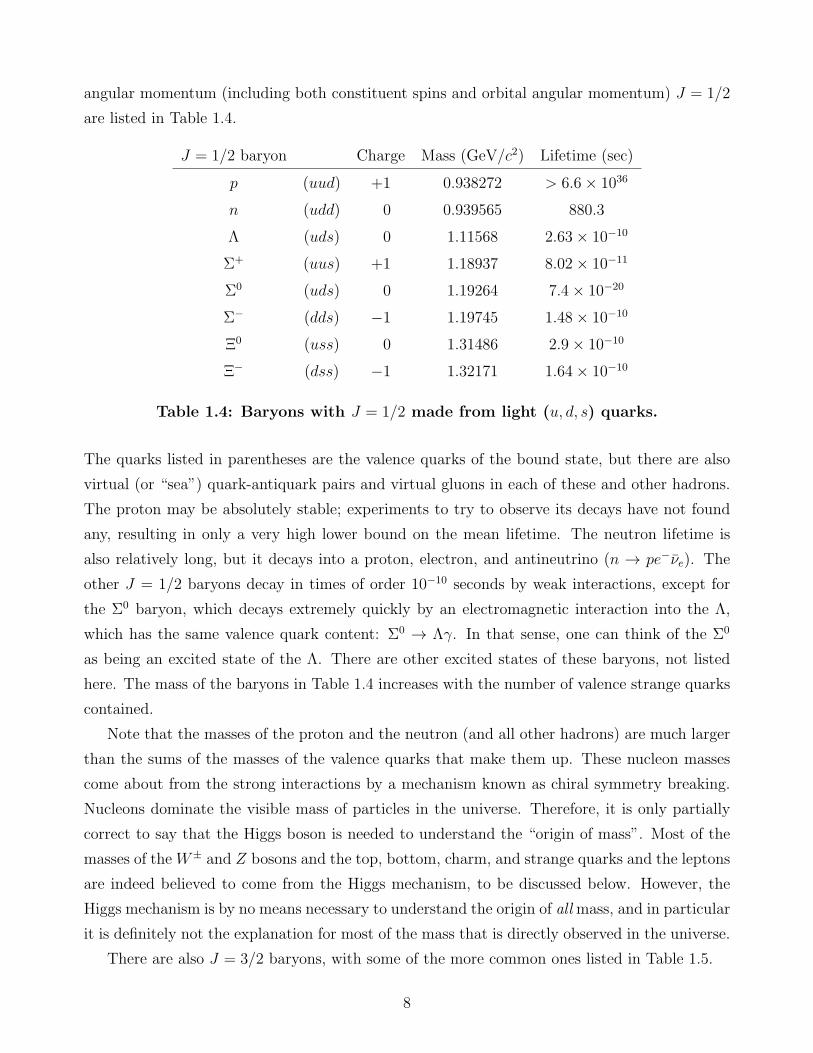
angular momentum (including both constituent spins and orbital angular momentum) J = 1/2

are listed in Table 1.4.

J = 1/2 baryon Charge Mass (GeV/c2) Lifetime (sec)

p (uud) +1 0.938272 > 6.6× 1036

n (udd) 0 0.939565 880.3

Λ (uds) 0 1.11568 2.63× 10−10

Σ+ (uus) +1 1.18937 8.02× 10−11

Σ0 (uds) 0 1.19264 7.4× 10−20

Σ− (dds) −1 1.19745 1.48× 10−10

Ξ0 (uss) 0 1.31486 2.9× 10−10

Ξ− (dss) −1 1.32171 1.64× 10−10

Table 1.4: Baryons with J = 1/2 made from light (u, d, s) quarks.

The quarks listed in parentheses are the valence quarks of the bound state, but there are also

virtual (or “sea”) quark-antiquark pairs and virtual gluons in each of these and other hadrons.

The proton may be absolutely stable; experiments to try to observe its decays have not found

any, resulting in only a very high lower bound on the mean lifetime. The neutron lifetime is

also relatively long, but it decays into a proton, electron, and antineutrino (n → pe−νe). The

other J = 1/2 baryons decay in times of order 10−10 seconds by weak interactions, except for

the Σ0 baryon, which decays extremely quickly by an electromagnetic interaction into the Λ,

which has the same valence quark content: Σ0 → Λγ. In that sense, one can think of the Σ0

as being an excited state of the Λ. There are other excited states of these baryons, not listed

here. The mass of the baryons in Table 1.4 increases with the number of valence strange quarks

contained.

Note that the masses of the proton and the neutron (and all other hadrons) are much larger

than the sums of the masses of the valence quarks that make them up. These nucleon masses

come about from the strong interactions by a mechanism known as chiral symmetry breaking.

Nucleons dominate the visible mass of particles in the universe. Therefore, it is only partially

correct to say that the Higgs boson is needed to understand the “origin of mass”. Most of the

masses of theW± and Z bosons and the top, bottom, charm, and strange quarks and the leptons

are indeed believed to come from the Higgs mechanism, to be discussed below. However, the

Higgs mechanism is by no means necessary to understand the origin of all mass, and in particular

it is definitely not the explanation for most of the mass that is directly observed in the universe.

There are also J = 3/2 baryons, with some of the more common ones listed in Table 1.5.

8

J = 3/2 baryon Charge Mass (GeV/c2) Γ (GeV/c2) Lifetime (seconds)

∆++ (uuu) +2 1.232 0.117 5.6× 10−24

∆+ (uud) +1 "" "" ""

∆0 (udd) 0 "" "" ""

∆− (ddd) −1 "" "" ""

Σ∗+ (suu) +1 1.383 0.036 1.8× 10−23

Σ∗0 (sud) 0 1.384 0.036 1.8× 10−23

Σ∗− (sdd) −1 1.387 0.039 1.7× 10−23

Ξ∗0 (ssu) 0 1.532 0.0091 7.2× 10−23

Ξ∗− (ssd) −1 1.535 0.0099 6.6× 10−23

Ω− (sss) −1 1.672 8.0× 10−15 8.21× 10−11

Table 1.5: J = 3/2 baryons.

The RPP uses a slightly different notation for the Σ∗ and Ξ∗ J = 3/2 baryons. Instead of the∗ notation to differentiate these states from the corresponding J = 1/2 baryons with the same

quantum numbers, the RPP chooses to denote them by their approximate mass in MeV (as

determined by older experiments, so a little off from the present best values) in parentheses, so

Σ(1385) and Ξ(1530). Very narrow resonances correspond to very long-lived states; the Ω− is

by far the narrowest and most stable of the ten J = 3/2 baryon ground states listed.

There are also baryons containing heavy (c or b) quarks. The only ones that have been

definitively observed so far have J = 1/2 and contain exactly one heavy quark. The lowest lying

states with a charm quark include the Λ+c , Σ

++c , Σ+

c , Σ0c , Ξ

+c , Ξ

0c , and Ω0

c resonances with masses

ranging from 2.29 GeV/c2 to 2.7 GeV/c2, and those with a bottom quark include the Λ0b , Ξ

0b ,

Ξ−b , Ω

−b , Σ

+b , and Σ−

b , with masses ranging from 5.62 GeV/c2 to 5.82 GeV/c2. More information

about them can be found in the RPP. Again, there are other baryons, generally with heavier

masses, that can be thought of as excited states of the more common ones listed above.

Bound states of a valence quark and antiquark are called mesons. They always carry integer

total angular momentum J . The most common J = 0 mesons are listed in Table 1.6.

Here the bar over a quark name denotes the corresponding antiquark. The charged pions π± are

antiparticles of each other, as are the charged kaons K±, so they are exactly degenerate mass

pairs with the same lifetime. However, the K0 and K0 mesons are mixed and not quite exactly

degenerate in mass. One of the interaction eigenstates (K0L) is actually much longer-lived than

the other (K0S); the mean lifetimes are respectively 5.12 × 10−8 and 8.95× 10−11 seconds. The

lifetimes (and the widths) of the other J = 0 mesons are not listed here; you can find them

9

J = 0 meson Charge Mass (GeV/c2)

π0 (uu, dd) 0 0.134977

π± (ud); (du) ±1 0.139570

K± (us); (su) ±1 0.493677

K0, K0 (ds); (sd) 0 0.497614

η (uu, dd, ss) 0 0.54786

η′ (uu, dd, ss) 0 0.95778

Table 1.6: J = 0 mesons containing light (u, d, s) quarks and antiquarks.

yourself in the RPP.

Besides the J = 0 mesons listed above, there are counterparts containing a single heavy

(charm or bottom) quark or antiquark, with the other antiquark or quark light (up, down or

strange). The most common ones are listed in Table 1.7.

J = 0 meson Charge Mass (GeV/c2)

D0, D0 (cu); (uc) 0 1.8648

D± (cd); (dc) ±1 1.8696

D±s (cs); (sc) ±1 1.9683

B± (ub); (bu) ±1 5.279

B0, B0 (db); (bd) 0 5.280

B0s , B

0s (sb); (bs) 0 5.367

Table 1.7: J = 0 mesons containing one heavy and one light quark and antiquark.

There are also J = 0 mesons containing only charm and bottom quarks and antiquarks. The

ones with the lowest masses are listed in Table 1.8.

J = 0 meson Charge Mass (GeV/c2)

ηc “charmonium” (cc) 0 2.984

B±c (cb); (bc) ±1 6.275

ηb “bottomonium” (bb) 0 9.398

Table 1.8: J = 0 mesons containing a heavy quark and a heavy antiquark.

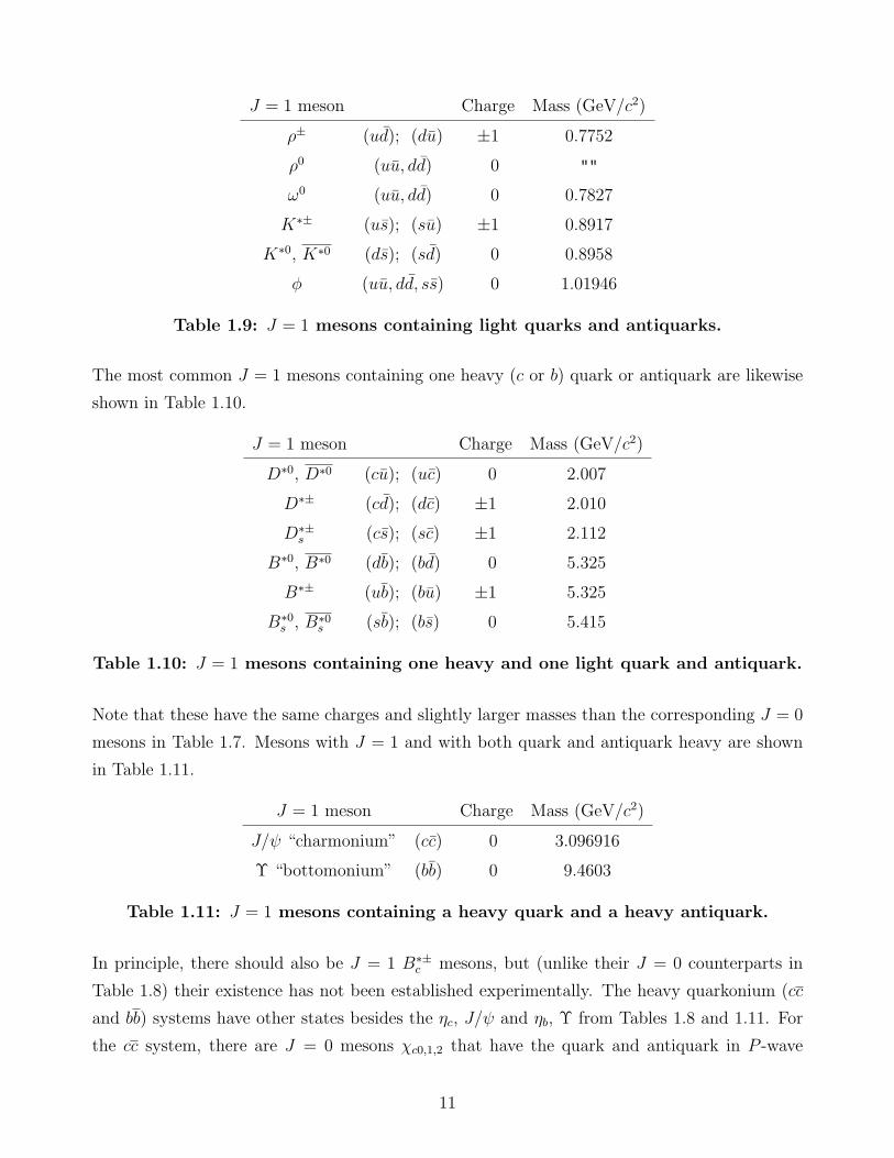
Vector (J = 1) mesons are also very important. Table 1.9 lists the most common ones that

contain only light (u, d, s) valence quarks and antiquarks.

10

J = 1 meson Charge Mass (GeV/c2)

ρ± (ud); (du) ±1 0.7752

ρ0 (uu, dd) 0 ""

ω0 (uu, dd) 0 0.7827

K∗± (us); (su) ±1 0.8917

K∗0, K∗0 (ds); (sd) 0 0.8958

φ (uu, dd, ss) 0 1.01946

Table 1.9: J = 1 mesons containing light quarks and antiquarks.

The most common J = 1 mesons containing one heavy (c or b) quark or antiquark are likewise

shown in Table 1.10.

J = 1 meson Charge Mass (GeV/c2)

D∗0, D∗0 (cu); (uc) 0 2.007

D∗± (cd); (dc) ±1 2.010

D∗±s (cs); (sc) ±1 2.112

B∗0, B∗0 (db); (bd) 0 5.325

B∗± (ub); (bu) ±1 5.325

B∗0s , B∗0

s (sb); (bs) 0 5.415

Table 1.10: J = 1 mesons containing one heavy and one light quark and antiquark.

Note that these have the same charges and slightly larger masses than the corresponding J = 0

mesons in Table 1.7. Mesons with J = 1 and with both quark and antiquark heavy are shown

in Table 1.11.

J = 1 meson Charge Mass (GeV/c2)

J/ψ “charmonium” (cc) 0 3.096916

Υ “bottomonium” (bb) 0 9.4603

Table 1.11: J = 1 mesons containing a heavy quark and a heavy antiquark.

In principle, there should also be J = 1 B∗±c mesons, but (unlike their J = 0 counterparts in

Table 1.8) their existence has not been established experimentally. The heavy quarkonium (cc

and bb) systems have other states besides the ηc, J/ψ and ηb, Υ from Tables 1.8 and 1.11. For

the cc system, there are J = 0 mesons χc0,1,2 that have the quark and antiquark in P -wave

11

orbital angular momentum states. There are also states ηc(2S), ψ(2S), ψ(3770), ψ(3872) that

are similar to the ηc and J/ψ, but with excited radial bound-state wavefunctions. Similarly,

in the bb system, there are excited bottomonium states Υ(2S), Υ(3S), Υ(4S), Υ(10860), and

Υ(11020) with J = 1, and P -wave orbital angular momentum states with total J = 0, χb0,1,2(1P )

and χb0,1,2(2P ). The spectroscopy of these states provides a striking confirmation of the quark

model for hadrons and of the strong force.

Much more detailed information on all of these hadronic bound states (and many others not

listed above), including the decay widths and the decay products, can be found in the RPP.

Theoretically, one also expects exotic mesons that are mostly “gluonium” or glueballs, that is,

bound states of gluons. However, these states are expected to mix with excited quark-antiquark

bound states, and they will be extremely difficult to identify experimentally.

In collider experiments, hadrons are most often produced in groups called jets. Roughly

speaking, each jet can be thought of as originating, at the shortest distance scales, from individ-

ual gluons and quarks (partons) which then hadronize by complicated processes into collections

of final state particles that share the energy and momentum of the original parton. The hadrons

in a given jet have momenta in approximately the same direction as their parent parton.

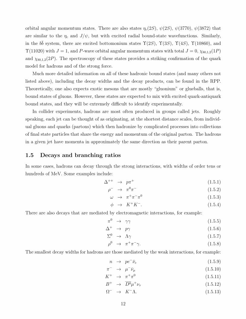
1.5 Decays and branching ratios

In some cases, hadrons can decay through the strong interactions, with widths of order tens or

hundreds of MeV. Some examples include:

∆++ → pπ+ (1.5.1)

ρ− → π0π− (1.5.2)

ω → π+π−π0 (1.5.3)

φ → K+K−. (1.5.4)

There are also decays that are mediated by electromagnetic interactions, for example:

π0 → γγ (1.5.5)

∆+ → pγ (1.5.6)

Σ0 → Λγ (1.5.7)

ρ0 → π+π−γ. (1.5.8)

The smallest decay widths for hadrons are those mediated by the weak interactions, for example:

n → pe−νe (1.5.9)

π− → µ−νµ (1.5.10)

K+ → π+π0 (1.5.11)

B+ → D0µ+ντ (1.5.12)

Ω− → K−Λ. (1.5.13)

12

The weak interactions are also entirely responsible for the decays of the charged leptons:

µ− → νµe−νe (1.5.14)

τ− → ντe−νe (1.5.15)

τ− → ντµ−νµ (1.5.16)

τ− → ντ + hadrons. (1.5.17)

Experimentally, the hadronic τ decays are classified by the number of charged hadrons present

in the final state, as either “1-prong” (if exactly one charged hadron), “3-prong” (if exactly three

charged hadrons), etc.

In most cases, a variety of different decay modes contribute to each total decay width. The

fraction that each final state contributes to the total decay width is known as the branching

ratio (or branching fraction), usually abbreviated as BR or B. As a randomly chosen example,

in the case of the ω meson the strong interaction accounts for most, but not all, of the decays:

BR(ω → π+π−π0) = (89.2± 0.7)% (strong) (1.5.18)

BR(ω → π0γ) = (8.3± 0.3)% (EM) (1.5.19)

BR(ω → π+π−) = (1.53± 0.13)% (EM) (1.5.20)

with other final states totaling less than 1%.

It is also common to present this information in terms of the partial widths into various final

states. If the total decay width for a parent particle X is Γ(X), then the partial decay width of

X into a particular final state Y is

Γ(X → Y ) = BR(X → Y )Γ(X). (1.5.21)

The sum of all of the branching ratios is equal to 1, and the sum of the partial widths is equal

to the total decay width.

There are two roads to enlightenment regarding the Standard Model and its future replace-

ment. The experimental road, which is highly successful as indicated by the impressive volume

and detail in the RPP, finds the answers to masses, decay rates, branching ratios, production

rates, and even more detailed information like kinematic and angular distributions directly from

data in high-energy collisions. The theoretical road aims to match these results onto predictions

of quantum field theories specified in terms of a small number of parameters. In the case of

electromagnetic interactions, quantum field theory is extremely successful, providing amazingly

accurate predictions for observable quantities such as magnetic moments and interaction rates.

In other applications, quantum field theory is only partly successful. For some calculations,

perturbation theory and other known methods are too difficult to carry out, or do not converge

even in principle. In some cases, lattice gauge theory provides useful information; this approach

13

is based on a discretized approximation to quantum field theory and stochastic methods. In

other cases, only rough or even qualitative results are possible. However, quantum field theory

is systematic and elegant, and provides understanding that is often elusive in the raw data. In

the following notes, we will try to understand some of the basic calculation methods of quantum

field theory as a general framework, and eventually the description of the Standard Model in

terms of it.

14

2 Special Relativity and Lorentz Transformations

2.1 Lorentz transformations

A successful description of elementary particles must be consistent with the two pillars of modern

physics: special relativity and quantum mechanics. Let us begin by reviewing some important

features of special relativity.

Spacetime has four dimensions. For any given event (for example, a firecracker explodes, or

a particle decays to two other particles) one can assign a four-vector position:

(ct, x, y, z) = (x0, x1, x2, x3) = xµ (2.1.1)

The Greek indices µ, ν, ρ, . . . run over the values 0, 1, 2, 3, and c is the speed of light in vacuum.

As a matter of terminology, xµ is an example of a contravariant four-vector.

The laws of physics should not depend on what coordinate system we use, as long as it is

an “inertial reference frame”, which means that the coordinates describing the position of a free

classical particle do not accelerate. This invariance of the laws of physics is a guiding principle

in making a sensible theory. It is often useful to change our coordinate system from one inertial

reference frame to another, according to

xµ → x′µ = Lµνx

ν . (2.1.2)

Here Lµν is a constant 4 × 4 real matrix that parameterizes the Lorentz transformation. It is

not arbitrary, however, as we will soon see. Such a change of coordinates is called a Lorentz

transformation.

As a simple example of a Lorentz transformation, suppose we rotate our coordinate system

about the z-axis by an angle α. Then in the new coordinate system:

x′µ = (ct′, x′, y′, z′) (2.1.3)

where

ct′ = ct

x′ = x cosα + y sinα

y′ = −x sinα + y cosα

z′ = z. (2.1.4)

Alternatively, we could go to a frame moving with respect to the original frame with velocity v

along the z direction, with the origins of the two frames coinciding at time t = t′ = 0. Then:

ct′ = γ(ct− βz)

15

x′ = x

y′ = y

z′ = γ(z − βct). (2.1.5)

where

β = v/c; γ = 1/√1− β2. (2.1.6)

Another way of rewriting this is to define the rapidity ρ by β = tanh ρ, so that γ = cosh ρ and

βγ = sinh ρ. Then we can rewrite eq. (2.1.5),

x′0 = x0 cosh ρ− x3 sinh ρx′1 = x1

x′2 = x2

x′3 = −x0 sinh ρ+ x3 cosh ρ. (2.1.7)

This change of coordinates is called a boost (with rapidity ρ and in the z direction).

Another example of a contravariant four-vector is given by the 4-momentum formed from

the energy E and spatial momentum ~p of a particle:

pµ = (E/c, ~p ). (2.1.8)

In the rest frame of a particle of mass m, its 4-momentum is given by pµ = (mc, 0, 0, 0). All

contravariant four-vectors transform the same way under a Lorentz transformation:

a′µ = Lµνa

ν . (2.1.9)

The 4-momentum of a particle is related to its mass by the Lorentz transformation that relates

the frame of reference in which it is measured and the rest frame. In the example of eq. (2.1.5),

one has:

Lµν =

γ 0 0 −βγ0 1 0 00 0 1 0−βγ 0 0 γ

, (2.1.10)

and the inverse Lorentz transformation is

aµ = (L−1)µνa′ν , (L−1)µν =

γ 0 0 βγ0 1 0 00 0 1 0βγ 0 0 γ

. (2.1.11)

16

A key property of special relativity is that for any two events one can define a proper interval,

which is independent of the Lorentz frame, and which tells us how far apart the two events are

in a coordinate-independent sense. So, consider two events occurring at xµ and xµ + dµ, where

dµ is some four-vector displacement. The proper interval between the events is

(∆τ)2 = (d0)2 − (d1)2 − (d2)2 − (d3)2 = gµνdµdν (2.1.12)

where

gµν =

1 0 0 00 −1 0 00 0 −1 00 0 0 −1

(2.1.13)

is known as the metric tensor. Here, and from now on, we adopt the Einstein summation

convention, in which repeated indices µ, ν, . . . are taken to be summed over. It is an assumption

of special relativity that gµν is the same in every inertial reference frame.

The existence of the metric tensor allows us to define covariant four-vectors by lowering an

index:

xµ = gµνxν = (ct,−x,−y,−z), (2.1.14)

pµ = gµνpν = (E/c,−px,−py,−pz). (2.1.15)

Furthermore, one can define an inverse metric gµν so that

gµνgνρ = δµρ , (2.1.16)

where δµν = 1 if µ = ν, and otherwise = 0. It follows that

gµν =

1 0 0 00 −1 0 00 0 −1 00 0 0 −1

. (2.1.17)

Then one has, for any vector aµ,

aµ = gµνaν ; aµ = gµνaν . (2.1.18)

It follows that covariant four-vectors transform as

a′µ = Lµνaν (2.1.19)

where (note the positions of the indices!)

Lµν = gµρg

νσLρσ. (2.1.20)

17

Because one can always use the metric to go between contravariant and covariant four-vectors,

people often use a harmlessly sloppy terminology and neglect the distinction, simply referring

to them as four-vectors.

If aµ and bµ are any four-vectors, then

aµbνgµν = aµbνgµν = aµb

µ = aµbµ ≡ a · b (2.1.21)

is a scalar quantity. For example, if pµ and qµ are the four-momenta of any two particles, then

p · q is a Lorentz-invariant; it does not depend on which inertial reference frame it is measured

in. In particular, a particle with mass m satisfies the on-shell condition

p2 = pµpµ = E2/c2 − ~p 2 = m2c2. (2.1.22)

The Lorentz invariance of dot products of pairs of 4-momenta, plus the conservation of total four-

momentum, plus the on-shell condition (2.1.22), is enough to solve most problems in relativistic

kinematics.

2.2 Relativistic kinematics

Let us pause to illustrate this with an example. Consider the situation of two particles, each of

mass m, colliding. Suppose the result of the collision is two final-state particles each of mass

M . Let us find the threshold energy and momentum 4-vectors for this process in the COM

(center-of-momentum) frame and in the frame in which one of the initial-state particles is at

rest. Throughout most of the following, we will take c = 1, by a choice of units.

Relativistic kinematics problems are often more easily analyzed in the COM frame, so let

us consider that case first. Without loss of generality, we can take the colliding initial-state

particles to be moving along the z-axis. Then their 4-momenta are:

pµ1 = (E, 0, 0,√E2 −m2) (2.2.1)

pµ2 = (E, 0, 0, −√E2 −m2). (2.2.2)

The spatial momenta are required to be opposite by the definition of the COM frame, which in

turn requires the energies to be the same, using eq. (2.1.22) and the fact that the masses are

assumed equal. The total 4-momentum of the initial state is pµ = (2E, 0, 0, 0), and so this must

be equal to the total 4-momentum of the final state in the COM frame as well. Furthermore,

p2 = 4E2 (2.2.3)

is a Lorentz invariant, the same in any inertial frame.

18

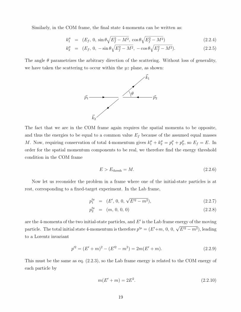
Similarly, in the COM frame, the final state 4-momenta can be written as:

kµ1 = (Ef , 0, sin θ√E2

f −M2, cos θ√E2

f −M2) (2.2.4)

kµ2 = (Ef , 0, − sin θ√E2

f −M2, − cos θ√E2

f −M2). (2.2.5)

The angle θ parametrizes the arbitrary direction of the scattering. Without loss of generality,

we have taken the scattering to occur within the yz plane, as shown:

~p1 ~p2

~k1

~k2

θ

The fact that we are in the COM frame again requires the spatial momenta to be opposite,

and thus the energies to be equal to a common value Ef because of the assumed equal masses

M . Now, requiring conservation of total 4-momentum gives kµ1 + kµ2 = pµ1 + pµ2 , so Ef = E. In

order for the spatial momentum components to be real, we therefore find the energy threshold

condition in the COM frame

E > Ethresh =M. (2.2.6)

Now let us reconsider the problem in a frame where one of the initial-state particles is at

rest, corresponding to a fixed-target experiment. In the Lab frame,

p′µ1 = (E ′, 0, 0,√E ′2 −m2), (2.2.7)

p′µ2 = (m, 0, 0, 0) (2.2.8)

are the 4-momenta of the two initial-state particles, and E ′ is the Lab frame energy of the moving

particle. The total initial state 4-momentum is therefore p′µ = (E ′+m, 0, 0,√E ′2 −m2), leading

to a Lorentz invariant

p′2 = (E ′ +m)2 − (E ′2 −m2) = 2m(E ′ +m). (2.2.9)

This must be the same as eq. (2.2.3), so the Lab frame energy is related to the COM energy of

each particle by

m(E ′ +m) = 2E2. (2.2.10)

19

Because we already found E > M , the Lab frame threshold energy condition for the scattering

event to be possible is m(E ′ +m) > 2M2, or

E ′ > E ′thresh =

2M2 −m2

m. (2.2.11)

Let us also relate the Lab frame 4-momenta to those in the COM frame. To find the Lorentz

transformation needed to go from the COM frame to the Lab frame, consider the 0, 3 components

of the equation p′µ2 = Λµνp

ν2:

(m0

)=(γ βγβγ γ

)(E

−√E2 −m2

). (2.2.12)

It follows that

β =√1−m2/E2 =

√E ′ −mE ′ +m

, (2.2.13)

γ =1√

1− β2= E/m =

√E ′ +m

2m, (2.2.14)

βγ =√E2/m2 − 1 =

√E ′ −m2m

. (2.2.15)

Now we can apply this Lorentz boost to the final-state momenta as found in the COM frame to

obtain the Lab frame momenta. For the first final-state particle:

k′µ1 =

γ 0 0 βγ0 1 0 00 0 1 0βγ 0 0 γ

E0

sin θ√E2 −M2

cos θ√E2 −M2

(2.2.16)

= (E2/m)

1 + cos θ√1−m2/E2

√1−M2/E2

0sin θ (m/E)

√1−M2/E2

√1−m2/E2 + cos θ

√1−M2/E2

. (2.2.17)

Note that for M > m, the z-component of the momentum is always positive (in the same

direction as the incoming particle in the Lab frame), regardless of the sign of cos θ. (The

other final-state momentum is obtained by just flipping the signs of cos θ and sin θ.) The Lab-

frame scattering angle with respect to the original collision axis (the z-axis in both frames) is

determined by

tan θ′ =(m/E) sin θ√

1−m2/E2/√1−M2/E2 + cos θ

. (2.2.18)

For fixed θ in the COM frame, |θ′| in the Lab frame decreases with increasing E/m, as the

produced particles go more in the forward direction.

20

Notice from eqs. (2.2.6) and (2.2.11) that while the production of a pair of heavy particles

of mass M requires beam energies in symmetric collisions that scale like M , in fixed-target

collisions the energy required scales like 2M2/m ≫ M , where m is the beam particle mass.

This is why fixed-target collisions are no longer an option for frontier physics discoveries of very

heavy particles or high-energy phenomena.

In collider applications, it is common to see the direction of a final-state particle with respect

to the colliding beams described either by the pseudo-rapidity η or the longitudinal rapidity y.

Suppose that the two colliding beams are oriented so that Beam 1 is going in the z direction

and Beam 2 is going in the −z direction. A final state particle (or group of particles) emerging

at an angle θ with respect to Beam 1 in general has a four-vector momentum given by:

pµ = (E, pT cosφ, pT sinφ, pz), (2.2.19)

where pT = |~p| sin θ is the transverse momentum, pz = |~p| cos θ is the longitudinal momentum,

and E =√|~p|2 +m2 is the energy, with m the mass and ~p the three-vector momentum. (In

hadron colliders, this four-vector is generally defined in the lab frame, not in the center-of-

momentum frame of the scattering event, which is often unknown.) Then the pseudo-rapidity

is defined by

η =1

2ln

(|~p|+ pz|~p| − pz

)= − ln [tan(θ/2)] . (2.2.20)

Thus η = 0 corresponds to a particle coming out perpendicular to the beam line (θ = 90),

while η = ±∞ correspond to the directions along the beams (θ = 0, 180). Particles at small |η|(less than 1 or 2 or so, depending on the situation) are said to be central, while those at large

|η| are said to be forward. Note that the pseudo-rapidity depends only on the direction of the

particle, not on its energy. The longitudinal rapidity is defined somewhat similarly by

y =1

2ln

(E + pzE − pz

). (2.2.21)

In fact, η = y in the special case of a massless particle, and they are very nearly equal for a

particle whose energy is large compared to its mass. However, in general y does depend on the

energy. For the same particle, the ordinary rapidity is given by:

ρ =1

2ln

(E + |~p|E − |~p|

). (2.2.22)

The quantity y is the rapidity of the boost needed to move to a frame where the particle has no

longitudinal momentum along the beam direction, while ρ is the rapidity of the boost needed

to move to the particle’s rest frame. Confusingly, it has become a standard abuse of language

21

among collider physicists to call y simply the rapidity, and among non-collider physicists it is

common to see the letter η used to refer to the ordinary rapidity, called ρ here. Some care is

needed to ensure that one is using and interpreting these quantities consistently.

2.3 Tensors and Lorentz invariant quantities

Now let us return to the study of the properties of Lorentz transformations. The Lorentz-

invariance of equation (2.1.21) implies that, if aµ and bµ are constant four-vectors, then

gµνa′µb′ν = gµνa

µbν , (2.3.1)

so that

gµνLµρL

νσa

ρbσ = gρσaρbσ. (2.3.2)

Since aµ and bν are arbitrary, it must be that:

gµνLµρL

νσ = gρσ. (2.3.3)

This is the fundamental constraint that a Lorentz transformation matrix must satisfy. In matrix

form, it could be written as LT gL = g. If we contract eq. (2.3.3) with gρκ, we obtain

LνκLν

σ = δκσ (2.3.4)

Applying this to eqs. (2.1.2) and (2.1.19), we find that the inverse Lorentz transformation of

any four-vector is

aν = a′µLµν (2.3.5)

aν = a′µLµν (2.3.6)

Let us now consider some more particular Lorentz transformations. To begin, we note

that as a matrix, det(L) = ±1. (See homework problem.) An example of a “large” Lorentz

transformation with det(L) = −1 is:

Lµν =

−1 0 0 00 1 0 00 0 1 00 0 0 1

. (2.3.7)

This just flips the sign of the time coordinate, and is therefore known as time reversal:

x′0 = −x0 x′1 = x1 x′2 = x2 x′3 = x3. (2.3.8)

22

Another “large” Lorentz transformation is parity, or space inversion:

Lµν =

1 0 0 00 −1 0 00 0 −1 00 0 0 −1

, (2.3.9)

so that:

x′0 = x0 x′1 = −x1 x′2 = −x2 x′3 = −x3. (2.3.10)

It was once thought that the laws of physics have to be invariant under these operations. How-

ever, it was shown experimentally in the 1950’s that parity is violated in the weak interactions,

specifically in the weak decays of the 60Co nucleus and the K± mesons. Likewise, experiments

in the 1960’s on the decays of K0 mesons showed that time-reversal invariance is violated (at

least if very general properties of quantum mechanics and special relativity are assumed).

However, all experiments up to now are consistent with invariance of the laws of physics

under the subset of Lorentz transformations that are continuously connected to the identity;

these are known as “proper” Lorentz transformations and have det(L) = +1. They can be built

up out of infinitesimal Lorentz transformations:

Lµν = δµν + ωµ

ν +O(ω2), (2.3.11)

where we agree to drop everything with more than one ωµν . Then, according to eq. (2.3.3),

gµν(δµρ + ωµ

ρ + . . .)(δνσ + ωνσ + . . .) = gρσ, (2.3.12)

or

gρσ + ωσρ + ωρσ + . . . = gρσ. (2.3.13)

Therefore

ωσρ = −ωρσ (2.3.14)

is an antisymmetric 4×4 matrix, with 4 ·3/2 ·1 = 6 independent entries. These correspond to 3

rotations (ρ, σ = 1, 2 or 1,3 or 2,3) and 3 boosts (ρ, σ = 0, 1 or 0,2 or 0,3). It is a mathematical

fact that any Lorentz transformation can be built up out of repeated infinitesimal boosts and

rotations, combined with the operations of time-reversal and space inversion.

Lorentz transformations obey the mathematical properties of a group, known as the Lorentz

group. The subset of Lorentz transformations that can be built out of repeated infinitesimal

boosts and rotations form a smaller group, called the proper Lorentz group. In the Standard

23

Model of particle physics and generalizations of it, all interesting objects, including operators,

states, particles, and fields, transform as well-defined representations of the Lorentz group. We

will study these group representations in more detail later.

So far we have considered constant four-vectors. However, one can also consider four-vectors

that depend on position in spacetime. For example, suppose that F (x) is a scalar function of

xµ. It is usual to leave the index µ off of xµ when it is used as the argument of a function, so

F (x) really means F (x0, x1, x2, x3). Under a Lorentz transformation from coordinates xµ → x′µ,

at a given fixed point in spacetime the value of the function F ′ reported by an observer using

the primed coordinate system is taken to be equal to the value of the original function F in the

original coordinates:

F ′(x′) = F (x). (2.3.15)

Then

∂µF ≡∂F

∂xµ=

(1

c

∂F

∂t, ~∇F

)(2.3.16)

is a covariant four-vector. This is because:

(∂µF )′(x′) ≡ ∂

∂x′µF ′(x′) =

∂xν

∂x′µ∂

∂xνF (x) = Lµ

ν(∂νF )(x), (2.3.17)

showing that it transforms according to eq. (2.1.19). [The second equality uses the chain rule

and eq. (2.3.15); the last equality uses eq. (2.3.5) with aµ = xµ.] By raising the index, one

obtains a contravariant four-vector function

∂µF = gµν∂νF =

(1

c

∂F

∂t,−~∇F

). (2.3.18)

One can obtain another scalar function by acting twice with the 4-dimensional derivative

operator on F , contracting the indices on the derivatives:

∂µ∂µF =1

c2∂2F

∂t2−∇2F. (2.3.19)

The object −∂µ∂µF is a 4-dimensional generalization of the Laplacian.

A tensor is an object that can carry an arbitrary number of spacetime vector indices, and

transforms appropriately when one goes to a new reference frame. The objects gµν and gµν and δµν

are constant tensors. Four-vectors and scalar functions and 4-derivatives of them are also tensors.

In general, the defining characteristic of a tensor function T µ1µ2...ν1ν2...

(x) is that under a change of

reference frame, it transforms so that in the primed coordinate system, the corresponding tensor

T ′ is:

T ′µ1µ2...ν1ν2...

(x′) = Lµ1ρ1L

µ2ρ2 · · ·Lν1

σ1Lν2σ2 · · ·T ρ1ρ2...

σ1σ2...(x). (2.3.20)

24

A special and useful constant tensor is the totally antisymmetric Levi-Civita tensor:

ǫµνρσ =

+1 if µνρσ is an even permutation of 0123−1 if µνρσ is an odd permutation of 01230 otherwise

(2.3.21)

One use for the Levi-Civita tensor is in understanding the Lorentz invariance of four-

dimensional integration. Define 4 four-vectors so that in a particular frame they are given

by the infinitesimal differentials:

Aµ = (cdt, 0, 0, 0); (2.3.22)

Bµ = (0, dx, 0, 0); (2.3.23)

Cµ = (0, 0, dy, 0); (2.3.24)

Dµ = (0, 0, 0, dz). (2.3.25)

Then the 4-dimensional volume element

d4x ≡ dx0dx1dx2dx3 = AµBνCρDσǫµνρσ (2.3.26)

is Lorentz-invariant, since in the last expression it has no uncontracted four-vector indices. It

follows that if F (x) is a Lorentz scalar function of xµ, then the integral

I[F ] =∫d4xF (x) (2.3.27)

is invariant under Lorentz transformations. This is good because eventually we will learn to

define theories in terms of such an integral, known as the action.

2.4 Maxwell’s equations and electromagnetism

An example of a relativistic theory that we are familiar with is electricity and magnetism. It

is instructive to recast Maxwell’s equations into a manifestly relativistic form. This will give

us familiarity with four-component gauge field formulation of the relativistic wave equations

governing electromagnetic fields. We will also see the relativistic version of gauge invariance

and concept of gauge transformations for the electromagnetic field, which will be explored more

completely in later sections.

Recall that Maxwell’s equations can be written in the form:

~∇ · ~E = eρ, (2.4.1)

~∇× ~B − ∂ ~E

∂t= e ~J, (2.4.2)

~∇ · ~B = 0, (2.4.3)

~∇× ~E +∂ ~B

∂t= 0, (2.4.4)

25

where ρ is the local charge density and ~J is the current density, with the magnitude of the

electron’s charge, e, factored out. These equations can be rewritten in a manifestly relativistic

form, using the following observations. First, suppose we add together the equations obtained

by taking ∂/∂t of eq. (2.4.1) and ~∇· of eq. (2.4.2). Since the divergence of a curl vanishes

identically, this yields the Law of Local Conservation of Charge:

∂ρ

∂t+ ~∇ · ~J = 0. (2.4.5)

To put this into a Lorentz-invariant form, we can form a four-vector charge and current density:

Jµ = (ρ, ~J ), (2.4.6)

so that eq. (2.4.5) becomes

∂µJµ = 0. (2.4.7)

Furthermore, eqs. (2.4.3) and (2.4.4) imply that we can write the electric and magnetic fields as

derivatives of the electric and magnetic potentials V and ~A:

~E = −~∇V − ∂ ~A

∂t, (2.4.8)

~B = ~∇× ~A. (2.4.9)

Now if we assemble the potentials into a four-vector:

Aµ = (V, ~A ), (2.4.10)

then eqs. (2.4.8) and (2.4.9) mean that we can write the electric and magnetic fields as compo-

nents of an antisymmetric tensor:

Fµν = ∂µAν − ∂νAµ (2.4.11)

=

0 Ex Ey Ez

−Ex 0 −Bz By

−Ey Bz 0 −Bx

−Ez −By Bx 0

. (2.4.12)

Now the Maxwell equations (2.4.1) and (2.4.2) correspond to the relativistic wave equation

∂µFµν = eJν , (2.4.13)

or equivalently,

∂µ∂µAν − ∂ν∂µAµ = eJν . (2.4.14)

26

The remaining Maxwell equations (2.4.3) and (2.4.4) are equivalent to the identity:

∂ρFµν + ∂µFνρ + ∂νFρµ = 0, (2.4.15)

for µ, ν, ρ = any of 0, 1, 2, 3. Note that this equation is automatically true because of eq. (2.4.11).

Also, because F µν is antisymmetric and partial derivatives commute, ∂µ∂νFµν = 0, so that the

Law of Local Conservation of Charge eq. (2.4.7) follows from eq. (2.4.13).

The potential Aµ(x) may be thought of as fundamental, and the fields ~E and ~B as derived

from it. The theory of electromagnetism as described by Aµ(x) is subject to a redundancy

known as gauge invariance. To see this, we note that eq. (2.4.14) is unchanged if we do the

transformation

Aµ(x)→ Aµ(x) + ∂µλ(x), (2.4.16)

where λ(x) is any function of position in spacetime. In components, this amounts to:

V → V +∂λ

∂t, (2.4.17)

~A → ~A− ~∇λ . (2.4.18)

This transformation leaves F µν (or equivalently ~E and ~B) unchanged. Therefore, the new Aµ

is just as good as the old Aµ for the purposes of describing a particular physical situation.

27

3 Relativistic Quantum Mechanics of Single Particles

3.1 Klein-Gordon and Dirac equations

Any realistic theory must be consistent with quantum mechanics. In this section, we consider

how to formulate a theory of quantum mechanics that is consistent with special relativity.

Suppose that Φ(x) is the wavefunction of a free particle in 4-dimensional spacetime. A

fundamental principle of quantum mechanics is that the time dependence of Φ is determined by

a Hamiltonian operator, according to:

HΦ = ih∂

∂tΦ. (3.1.1)

Now, the three-momentum operator is given by

~P = −ih~∇. (3.1.2)

BecauseH and ~P commute, one can take Φ to be one of the basis of wavefunctions for eigenstates

with energy and momentum eigenvalues E and ~p respectively:

HΦ = EΦ; ~PΦ = ~pΦ. (3.1.3)

One can now turn this into a relativistic Schrodinger wave equation for free particle states, by

using the fact that special relativity implies:

E =√m2c4 + ~p 2c2, (3.1.4)

where m is the mass of the particle. To make sense of this as an operator equation, we could

try expanding it in an infinite series, treating ~p 2 as small compared to m2c2:

ih∂

∂tΦ = mc2(1 +

~p 2

2m2c2− ~p 4

8m4c4+ . . .)Φ (3.1.5)

= [mc2 − h2

2m∇2 − h4

8m3c2(∇2)2 + . . .]Φ (3.1.6)

If we keep only the first two terms, then we recover the standard non-relativistic quantum

mechanics of a free particle; the first term mc2 is an unobservable constant contribution to the

Hamiltonian, proportional to the rest energy, and the second term is the usual non-relativistic

kinetic energy. However, the presence of an infinite number of derivatives leads to horrible

problems, including apparently non-local effects.

Instead, one can consider the operator H2 acting on Φ, avoiding the square root. It follows

that

H2Φ = E2Φ = (c2~p 2 +m2c4)Φ = (c2 ~P2+m2c4)Φ, (3.1.7)

28

so that:

−∂2Φ

∂t2= −∇2Φ +m2Φ. (3.1.8)

Here and from now on we have set c = 1 and h = 1 by a choice of units. This convention means

that mass, energy, and momentum all have the same units (GeV), while time and distance have

units of GeV−1, and velocity is dimensionless. These conventions greatly simplify the equations

of particle physics. One can always recover the usual metric system units using the following

conversion table for energy, mass, distance, and time, respectively:

1 GeV = 1.6022× 10−3 erg = 1.6022× 10−10 Joules, (3.1.9)

(1 GeV)/c2 = 1.7827× 10−24 g = 1.7827× 10−27 kg, (3.1.10)

(1 GeV)−1(hc) = 1.9733× 10−14 cm = 1.9733× 10−16 m, (3.1.11)

(1 GeV)−1h = 6.58212× 10−25 sec. (3.1.12)

Using eq. (2.3.19), the wave-equation eq. (3.1.8) can be rewritten in a manifestly Lorentz-

invariant way as

(∂µ∂µ +m2)Φ = 0. (3.1.13)

This relativistic generalization of the Schrodinger equation is known as the Klein-Gordon equa-

tion.

It is easy to guess the solutions of the Klein-Gordon equation. If we try:

Φ(x) = Φ0e−ik·x, (3.1.14)

where Φ0 is a constant and kµ is a four-vector, then ∂µΦ = −ikµΦ and so

∂µ∂µΦ = −kµkµΦ = −k2Φ. (3.1.15)

Therefore, we only need to impose k2 = m2 to have a solution. It is then easy to check that

this is an eigenstate of H and ~P with energy E = k0 and three-momentum ~p = ~k, satisfying

E2 = ~p 2 +m2.

However, there is a big problem with this. If kµ = (E, ~p ) gives a solution, then so does

kµ = (−E, ~p ). By increasing |~p |, one can have |E| arbitrarily large. This is a disaster, because

the energy is not bounded from below. If the particle can interact, it will make transitions from

higher energy states to lower energy states. This would seem to lead to the release of an infinite

amount of energy as the particle acquires a larger and larger three-momentum, without bound!

In 1927, Dirac suggested an alternative, based on the observation that the problem with the

Klein-Gordon equation seems to be that it is quadratic in H or equivalently ∂/∂t; this leads

29

to the sign ambiguity for E. Dirac could also have been† motivated by the fact that particles

like the electron have spin; since they have more than one intrinsic degree of freedom, trying to

explain them with a single wavefunction Φ(x) is doomed to failure. Instead, Dirac proposed to

write a relativistic Schrodinger equation, for a multi-component wavefunction Ψa(x), where the

spinor index a = 1, 2, . . . , n runs over the components. The wave equation should be linear in

∂/∂t; since relativity places t on the same footing as x, y, z, it should also be linear in derivatives

of the spatial coordinates. Therefore, the equation ought to take the form

i∂

∂tΨ = HΨ = (~α · ~P + βm)Ψ, (3.1.16)

where αx, αy, αz, and β are n× n matrices acting in “spinor space”.

To determine what ~α and β have to be, consider H2Ψ. There are two ways to evaluate the

result. First, by exactly the same reasoning as for the Klein-Gordon equation, one finds

− ∂2

∂t2Ψ = (−∇2 +m2)Ψ. (3.1.17)

On the other hand, expressing H in terms of the right-hand side of eq. (3.1.16), we find:

− ∂2

∂t2Ψ =

−

3∑

j,k=1

αjαk∂

∂xj∂

∂xk− im

∑

j

(αjβ + βαj)∂

∂xj+ β2m2

Ψ. (3.1.18)

Since partial derivatives commute, one can write:

3∑

j,k=1

αjαk∂

∂xj∂

∂xk=

1

2

3∑

j,k=1

(αjαk + αkαj)∂

∂xj∂

∂xk. (3.1.19)

Then comparing eqs. (3.1.17) and (3.1.18), one finds that the two agree if, for j, k = 1, 2, 3:

β2 = 1, (3.1.20)

αjβ + βαj = 0, (3.1.21)

αjαk + αkαj = 2δjk. (3.1.22)

The simplest solution turns out to require n = 4 spinor indices. This may be somewhat

surprising, since naively one only needs n = 2 to describe a spin-1/2 particle like the electron. As

we will see, the Dirac equation automatically describes positrons as well as electrons, accounting

for the doubling. It is easiest to write the solution in terms of 2× 2 Pauli matrices:

σ1 =(0 11 0

), σ2 =

(0 −ii 0

), σ3 =

(1 00 −1

), and σ0 =

(1 00 1

). (3.1.23)

†Apparently, he realized this only in hindsight.

30

Then one can check that the 4× 4 matrices

β =(

0 σ0

σ0 0

), αj =

(−σj 00 σj

), (j = 1, 2, 3) (3.1.24)

obey the required conditions. The matrices β, αj are written in 2×2 block form, so “0” actually

denotes a 2 × 2 block of 0’s. Equation (3.1.16) is known as the Dirac equation, and the 4-

component object is known as a Dirac spinor. Note that the fact that Dirac spinor space is

4-dimensional, just like ordinary spacetime, is really just a coincidence.‡ One must be careful

not to confuse the two types of 4-dimensional spaces!

It is convenient and traditional to rewrite the Dirac equation in a nicer way by multiplying

it on the left by the matrix β, and defining

γ0 = β, γj = βαj, (j = 1, 2, 3). (3.1.25)

The result is[i(γ0

∂

∂x0+ γ1

∂

∂x1+ γ2

∂

∂x2+ γ3

∂

∂x3)−m

]Ψ = 0, (3.1.26)

or, even more nicely:

(iγµ∂µ −m)Ψ = 0. (3.1.27)

The γµ matrices are explicitly given, in 2× 2 blocks, by:

γ0 =(

0 σ0

σ0 0

), γj =

(0 σj

−σj 0

), (j = 1, 2, 3). (3.1.28)

[The solution found above for the γµ is not unique. To see this, suppose U is any constant

unitary 4× 4 matrix satisfying U †U = 1. Then the Dirac equation implies:

U(iγµ∂µ −m)U †UΨ = 0, (3.1.29)

from which it follows that, writing γ′µ = UγµU †, and Ψ′ = UΨ,

(iγ′µ∂µ −m)Ψ′ = 0. (3.1.30)

So, the new γ′µ matrices together with the new spinor Ψ′ are just as good as the old pair γµ,Ψ;

there are an infinite number of different, equally valid choices. The set we’ve given above is

called the chiral or Weyl representation. Another popular choice used by some textbooks (but

not here) is the Pauli-Dirac representation.]

‡For example, if we lived in 10 dimensional spacetime, it turns out that Dirac spinors would have 32 compo-nents.

31

Many problems involving fermions in high-energy physics involve many gamma matrices

dotted into partial derivatives or momentum four-vectors. To keep the notation from getting

too bloated, it is often useful to use the Feynman slash notation:

γµaµ = /a (3.1.31)

for any four-vector aµ. Then the Dirac equation takes the even more compact form:

(i/∂ −m)Ψ = 0. (3.1.32)

Some important properties of the γµ matrices are:

γ0† = γ0, γj† = −γj, (j = 1, 2, 3), (3.1.33)

γ0㵆γ0 = γµ, (3.1.34)

Tr(γµγν) = 4gµν , (3.1.35)

γµγµ = 4, (3.1.36)

γµγν + γνγµ = γµ, γν = 2gµν . (3.1.37)

Note that on the right-hand sides of each of eqs. (3.1.36) and (3.1.37), there is an implicit 4× 4

unit matrix. It turns out that one almost never needs to know the explicit form of the γµ.

Instead, the equations above can be used to derive identities needed in practical work. (You

will get some practice with this from the homework.)

How does a Dirac spinor Ψa(x) transform under a Lorentz transformation? It carries no

vector index, so it is not a tensor. On the other hand, the fact that the Hamiltonian “mixes

up” the components of Ψa(x) is a clue that it doesn’t transform like an ordinary scalar function

either. Instead, we might expect that the spinor reported by an observer in the primed frame

is given by

Ψ′(x′) = ΛΨ(x), (3.1.38)

where Λ is a 4× 4 matrix that depends on the Lorentz transformation matrix Lµν . In fact, you

will show for homework that for an infinitesimal Lorentz transformation Lµν = δµν + ωµ

ν , one

has:

Ψ′(x′) = (1− i

2ωµνS

µν)Ψ(x), (3.1.39)

where

Sµν =i

4[γµ, γν ]. (3.1.40)

32

To obtain the result for a non-infinitesimal proper Lorentz transformation, we can apply

the same infinitesimal transformation a large number of times N , with N → ∞. Letting

Ωµν = Nωµν , we obtain, after N iterations of the Lorentz transformation parameterized by ωµν :

Lµν = (δµν + Ωµ

ν/N)N → [exp(Ω)]µν (3.1.41)

as N →∞. Here we are using the identity:

limN→∞

(1 + x/N)N = exp(x), (3.1.42)

with the exponential of a matrix to be interpreted in the power series sense:

exp(M) = 1 +M +M2/2 +M3/6 + . . . . (3.1.43)

For the Dirac spinor, one has in the same way:

Ψ′(x′) =(1− i

2ΩµνS

µν/N)N

Ψ(x) → exp(− i2ΩµνS

µν)Ψ(x). (3.1.44)

So, we have found the Λ that appears in eq. (3.1.38) corresponding to the Lµν that appears in

eq. (3.1.41):

Λ = exp(− i2ΩµνS

µν). (3.1.45)

As an example, consider a boost in the z direction:

Ωµν =

0 0 0 −ρ0 0 0 00 0 0 0−ρ 0 0 0

. (3.1.46)

Then

Ω2 =

ρ2 0 0 00 0 0 00 0 0 00 0 0 ρ2

, Ω3 =

0 0 0 −ρ30 0 0 00 0 0 0−ρ3 0 0 0

, etc. (3.1.47)

so that from eqs. (3.1.41) and (3.1.43),

Lµν =

1 0 0 00 1 0 00 0 1 00 0 0 1

+

(ρ2

2+ρ4

24+ . . .

)

1 0 0 00 0 0 00 0 0 00 0 0 1

−

(ρ+

ρ3

6+ . . .

)

0 0 0 10 0 0 00 0 0 01 0 0 0

=

cosh ρ 0 0 − sinh ρ0 1 0 00 0 1 0

− sinh ρ 0 0 cosh ρ

, (3.1.48)

33

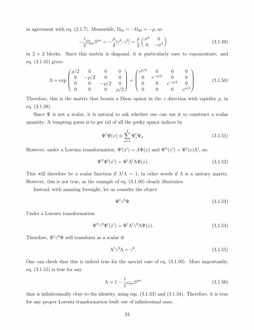
in agreement with eq. (2.1.7). Meanwhile, Ω03 = −Ω30 = −ρ, so

− i2ΩµνS

µν = −ρ4[γ0, γ3] =

ρ

2

(σ3 00 −σ3

)(3.1.49)

in 2 × 2 blocks. Since this matrix is diagonal, it is particularly easy to exponentiate, and

eq. (3.1.45) gives:

Λ = exp

ρ/2 0 0 00 −ρ/2 0 00 0 −ρ/2 00 0 0 ρ/2

=

eρ/2 0 0 00 e−ρ/2 0 00 0 e−ρ/2 00 0 0 eρ/2

. (3.1.50)

Therefore, this is the matrix that boosts a Dirac spinor in the z direction with rapidity ρ, in

eq. (3.1.38).

Since Ψ is not a scalar, it is natural to ask whether one can use it to construct a scalar

quantity. A tempting guess is to get rid of all the pesky spinor indices by

Ψ†Ψ(x) ≡4∑

a=1

Ψ†aΨa. (3.1.51)

However, under a Lorentz transformation, Ψ′(x′) = ΛΨ(x) and Ψ′†(x′) = Ψ†(x)Λ†, so:

Ψ′†Ψ′(x′) = Ψ†Λ†ΛΨ(x). (3.1.52)

This will therefore be a scalar function if Λ†Λ = 1, in other words if Λ is a unitary matrix.

However, this is not true, as the example of eq. (3.1.50) clearly illustrates.

Instead, with amazing foresight, let us consider the object

Ψ†γ0Ψ. (3.1.53)

Under a Lorentz transformation:

Ψ′†γ0Ψ′(x′) = Ψ†Λ†γ0ΛΨ(x). (3.1.54)

Therefore, Ψ†γ0Ψ will transform as a scalar if:

Λ†γ0Λ = γ0. (3.1.55)

One can check that this is indeed true for the special case of eq. (3.1.50). More importantly,

eq. (3.1.55) is true for any

Λ = 1− i

2ωµνS

µν (3.1.56)

that is infinitesimally close to the identity, using eqs. (3.1.33) and (3.1.34). Therefore, it is true

for any proper Lorentz transformation built out of infinitesimal ones.

34

Motivated by this, one defines, for any Dirac spinor Ψ,

Ψ ≡ Ψ†γ0. (3.1.57)

One should think of Ψ as a column vector in spinor space, and Ψ as a row vector. Then their

inner product

ΨΨ, (3.1.58)

with all spinor indices contracted, transforms as a scalar function under proper Lorentz trans-

formations. Similarly, one can show that

ΨγµΨ (3.1.59)

transforms as a four-vector. One should think of eq. (3.1.59) as a (row vector)×(matrix)×(column

vector) in spinor-index space, with a spacetime vector index µ hanging around.

3.2 Solutions of the Dirac equation

Our next task is to construct solutions to the Dirac equation. Let us separate out the xµ-

dependent part as a plane wave, by trying

Ψ(x) = u(p, s)e−ip·x. (3.2.1)

Here pµ is a four-vector momentum, with p0 = E > 0. A solution to the Dirac equation must

also satisfy the Klein-Gordon equation, so p2 = E2 − ~p 2 = m2. The object u(p, s) is a spinor,

labeled by the 4-momentum p and s. For now s just distinguishes between distinct solutions,

but it will turn out to be related to the spin. Plugging this into the Dirac equation (3.1.32), we

obtain a 4× 4 eigenvalue equation to be solved for u(p, s):

(/p−m)u(p, s) = 0. (3.2.2)

To simplify things, first consider this equation in the rest frame of the particle, where pµ =

(m, 0, 0, 0). In that frame,

m(γ0 − 1)u(p, s) = 0. (3.2.3)

Using the explicit form of γ0, we can therefore write in 2× 2 blocks:(−1 1

1 −1)u(p, s) = 0, (3.2.4)

where each “1” means a 2× 2 unit matrix. The solutions are clearly

u(p, s) =√m(χs

χs

), (3.2.5)

35

where χs can be any 2-vector, and the√m normalization is a convention. In practice, it is best

to choose the χs orthonormal, satisfying χ†sχr = δrs for r, s = 1, 2. A particularly nice choice is:

χ1 =(10

), χ2 =

(01

). (3.2.6)

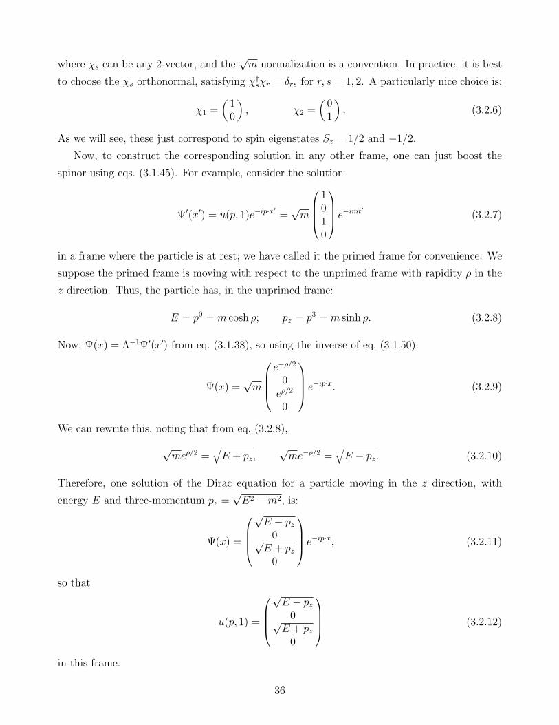
As we will see, these just correspond to spin eigenstates Sz = 1/2 and −1/2.Now, to construct the corresponding solution in any other frame, one can just boost the

spinor using eqs. (3.1.45). For example, consider the solution

Ψ′(x′) = u(p, 1)e−ip·x′

=√m

1010

e

−imt′ (3.2.7)

in a frame where the particle is at rest; we have called it the primed frame for convenience. We

suppose the primed frame is moving with respect to the unprimed frame with rapidity ρ in the

z direction. Thus, the particle has, in the unprimed frame:

E = p0 = m cosh ρ; pz = p3 = m sinh ρ. (3.2.8)

Now, Ψ(x) = Λ−1Ψ′(x′) from eq. (3.1.38), so using the inverse of eq. (3.1.50):

Ψ(x) =√m

e−ρ/2

0eρ/2

0

e

−ip·x. (3.2.9)

We can rewrite this, noting that from eq. (3.2.8),

√meρ/2 =

√E + pz,

√me−ρ/2 =

√E − pz. (3.2.10)

Therefore, one solution of the Dirac equation for a particle moving in the z direction, with

energy E and three-momentum pz =√E2 −m2, is:

Ψ(x) =

√E − pz0√

E + pz0

e

−ip·x, (3.2.11)

so that

u(p, 1) =

√E − pz0√

E + pz0

(3.2.12)

in this frame.

36

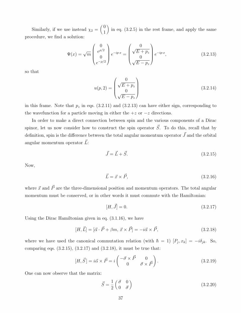
Similarly, if we use instead χ2 =(01

)in eq. (3.2.5) in the rest frame, and apply the same

procedure, we find a solution:

Ψ(x) =√m

0eρ/2

0e−ρ/2

e

−ip·x =

0√E + pz0√

E − pz

e

−ip·x, (3.2.13)

so that

u(p, 2) =

0√E + pz0√

E − pz

(3.2.14)

in this frame. Note that pz in eqs. (3.2.11) and (3.2.13) can have either sign, corresponding to

the wavefunction for a particle moving in either the +z or −z directions.

In order to make a direct connection between spin and the various components of a Dirac

spinor, let us now consider how to construct the spin operator ~S. To do this, recall that by

definition, spin is the difference between the total angular momentum operator ~J and the orbital

angular momentum operator ~L:

~J = ~L+ ~S. (3.2.15)

Now,

~L = ~x× ~P , (3.2.16)

where ~x and ~P are the three-dimensional position and momentum operators. The total angular

momentum must be conserved, or in other words it must commute with the Hamiltonian:

[H, ~J ] = 0. (3.2.17)

Using the Dirac Hamiltonian given in eq. (3.1.16), we have

[H, ~L] = [~α · ~P + βm, ~x× ~P ] = −i~α× ~P , (3.2.18)

where we have used the canonical commutation relation (with h = 1) [Pj, xk] = −iδjk. So,

comparing eqs. (3.2.15), (3.2.17) and (3.2.18), it must be true that:

[H, ~S ] = i~α× ~P = i

(−~σ × ~P 0

0 ~σ × ~P

). (3.2.19)

One can now observe that the matrix:

~S =1

2

(~σ 00 ~σ

)(3.2.20)

37

obeys eq. (3.2.19). So, it must be the spin operator acting on Dirac spinors.

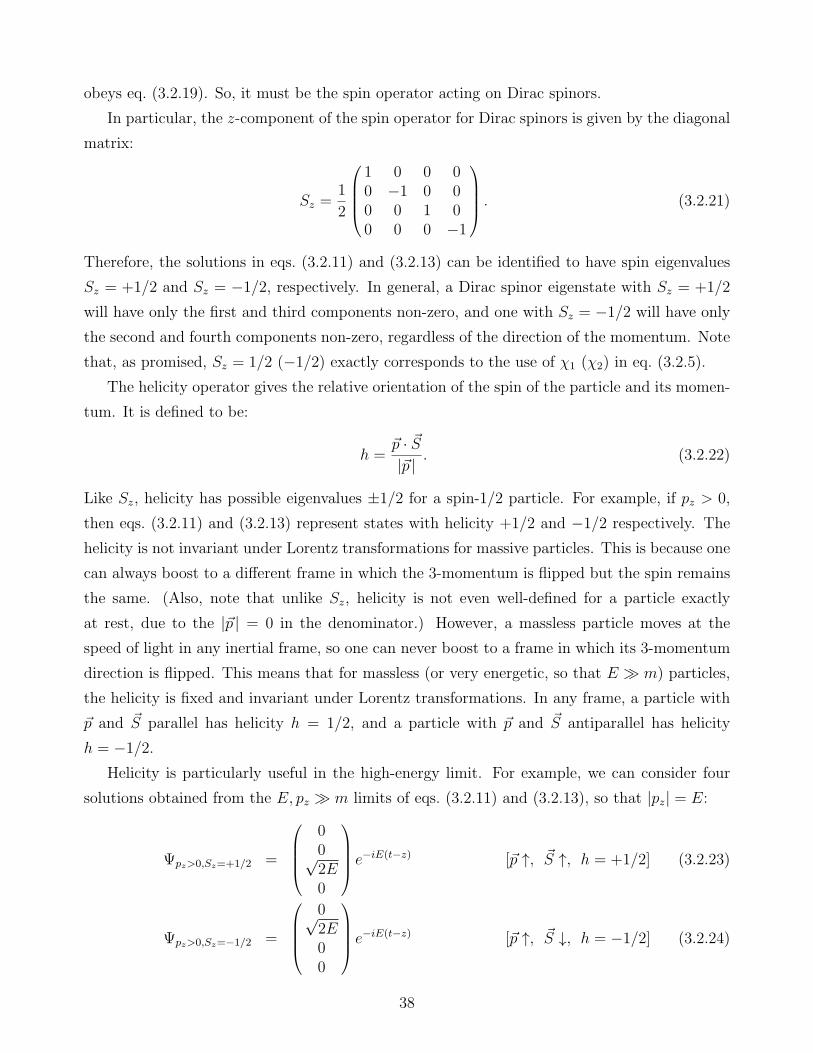
In particular, the z-component of the spin operator for Dirac spinors is given by the diagonal

matrix:

Sz =1

2

1 0 0 00 −1 0 00 0 1 00 0 0 −1

. (3.2.21)

Therefore, the solutions in eqs. (3.2.11) and (3.2.13) can be identified to have spin eigenvalues

Sz = +1/2 and Sz = −1/2, respectively. In general, a Dirac spinor eigenstate with Sz = +1/2

will have only the first and third components non-zero, and one with Sz = −1/2 will have only

the second and fourth components non-zero, regardless of the direction of the momentum. Note

that, as promised, Sz = 1/2 (−1/2) exactly corresponds to the use of χ1 (χ2) in eq. (3.2.5).

The helicity operator gives the relative orientation of the spin of the particle and its momen-

tum. It is defined to be:

h =~p · ~S|~p | . (3.2.22)

Like Sz, helicity has possible eigenvalues ±1/2 for a spin-1/2 particle. For example, if pz > 0,

then eqs. (3.2.11) and (3.2.13) represent states with helicity +1/2 and −1/2 respectively. The

helicity is not invariant under Lorentz transformations for massive particles. This is because one

can always boost to a different frame in which the 3-momentum is flipped but the spin remains

the same. (Also, note that unlike Sz, helicity is not even well-defined for a particle exactly

at rest, due to the |~p | = 0 in the denominator.) However, a massless particle moves at the

speed of light in any inertial frame, so one can never boost to a frame in which its 3-momentum

direction is flipped. This means that for massless (or very energetic, so that E ≫ m) particles,

the helicity is fixed and invariant under Lorentz transformations. In any frame, a particle with

~p and ~S parallel has helicity h = 1/2, and a particle with ~p and ~S antiparallel has helicity

h = −1/2.Helicity is particularly useful in the high-energy limit. For example, we can consider four

solutions obtained from the E, pz ≫ m limits of eqs. (3.2.11) and (3.2.13), so that |pz| = E:

Ψpz>0,Sz=+1/2 =

00√2E0

e

−iE(t−z) [~p ↑, ~S ↑, h = +1/2] (3.2.23)

Ψpz>0,Sz=−1/2 =

0√2E00

e

−iE(t−z) [~p ↑, ~S ↓, h = −1/2] (3.2.24)

38

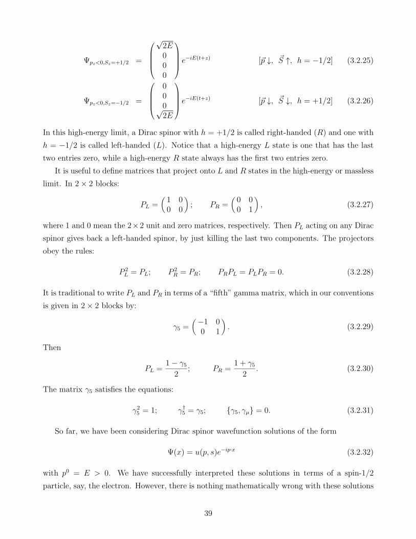
Ψpz<0,Sz=+1/2 =

√2E000

e

−iE(t+z) [~p ↓, ~S ↑, h = −1/2] (3.2.25)

Ψpz<0,Sz=−1/2 =

000√2E

e

−iE(t+z) [~p ↓, ~S ↓, h = +1/2] (3.2.26)

In this high-energy limit, a Dirac spinor with h = +1/2 is called right-handed (R) and one with

h = −1/2 is called left-handed (L). Notice that a high-energy L state is one that has the last

two entries zero, while a high-energy R state always has the first two entries zero.

It is useful to define matrices that project onto L and R states in the high-energy or massless

limit. In 2× 2 blocks:

PL =(1 00 0

); PR =

(0 00 1

), (3.2.27)

where 1 and 0 mean the 2×2 unit and zero matrices, respectively. Then PL acting on any Dirac

spinor gives back a left-handed spinor, by just killing the last two components. The projectors

obey the rules:

P 2L = PL; P 2

R = PR; PRPL = PLPR = 0. (3.2.28)

It is traditional to write PL and PR in terms of a “fifth” gamma matrix, which in our conventions

is given in 2× 2 blocks by:

γ5 =(−1 0

0 1

). (3.2.29)

Then

PL =1− γ5

2; PR =

1 + γ52

. (3.2.30)

The matrix γ5 satisfies the equations:

γ25 = 1; γ†5 = γ5; γ5, γµ = 0. (3.2.31)

So far, we have been considering Dirac spinor wavefunction solutions of the form

Ψ(x) = u(p, s)e−ip·x (3.2.32)

with p0 = E > 0. We have successfully interpreted these solutions in terms of a spin-1/2

particle, say, the electron. However, there is nothing mathematically wrong with these solutions

39

for pµ with p0 < 0 and p2 = m2. So, like the Klein-Gordon equation, the Dirac equation has the

embarrassment of negative energy solutions.

Dirac proposed to get around the problem of negative energy states by using the fact that

spin-1/2 particle are fermions. The Pauli exclusion principle dictates that two fermions cannot

occupy the same quantum state. Therefore, Dirac proposed that all of the negative energy states

are occupied. This prevents electrons with positive energy from making disastrous transitions

to the E < 0 states. The infinite number of filled E < 0 states is called the Dirac sea.

If one of the states in the Dirac sea becomes unoccupied, it leaves behind a “hole”. Since a

hole is the absence of an E < 0 state, it effectively has energy −E > 0. An electron has charge†

−e, so the hole corresponding to its absence effectively has the opposite charge, +e. Since both

electrons and holes obey p2 = m2, they have the same mass. Dirac’s proposal therefore predicts

the existence of “anti-electrons” or positrons, with positive energy and positive charge. The

positron was indeed discovered in 1932 in cosmic ray experiments.

Feynman and Stuckelberg noted that one can reinterpret the positron as a negative en-

ergy electron moving backwards in time, so that pµ → −pµ and ~S → −~S. According to this

interpretation, the wavefunction for a positron with 4-momentum pµ with p0 = E > 0 is

Ψ(x) = v(p, s)eip·x. (3.2.33)

Now, using the Dirac equation (3.1.32), v(p, s) must satisfy the eigenvalue equation:

(/p+m)v(p, s) = 0. (3.2.34)

We can now construct solutions to this equation just as before. First, in the rest (primed) frame

of the particle, we have in 2× 2 blocks:

(m mm m

)v(p, s) = 0. (3.2.35)

So, the solutions are

Ψ′(x′) =√m(ξs−ξs

)eimt′ (3.2.36)

for any two-vector ξs.

One must be careful in interpreting the quantum numbers of the positron solutions to the

Dirac equation. This is because the Hamiltonian, 3-momentum, and spin operators of a positron

described by the wavefunction eq. (3.2.33) are all given by the negative of the expressions one

†Here, e is always defined to be positive, so that the electron has charge −e. (Some references define e to benegative.)

40

would use for an electron wavefunction. Thus, acting on a positron wavefunction, one has

HΨ = −i ∂∂t

Ψ, (3.2.37)

~PΨ = i~∇Ψ, (3.2.38)

~SΨ = −1

2

(~σ 00 ~σ

)Ψ, (3.2.39)

where H, ~P , and ~S are the operators whose eigenvalues are to be interpreted as the energy,

3-momentum, and spin of the positive-energy positron antiparticle. Therefore, to describe a

positron with spin Sz = +1/2 or −1/2, one should use, respectively,

ξ1 =(01

); or ξ2 =

(10

), (3.2.40)

in eq. (3.2.36).

Now we can boost to the unprimed frame just as before, yielding the solutions:

v(p, 1) =

0√E + pz0

−√E − pz

, (3.2.41)

v(p, 2) =

√E − pz0

−√E + pz0

. (3.2.42)

Here v(p, 1) corresponds to a positron moving in the +z direction with 3-momentum pz and

energy E =√p2z +m2 and Sz = +1/2, hence helicity h = +1/2 if pz > 0. Similarly, v(p, 2)

corresponds to a positron with the same energy and 3-momentum, but with Sz = −1/2, andtherefore helicity h = −1/2 if pz > 0.

Note that for positron wavefunctions, PL projects onto states that describe right-handed

positrons in the high-energy limit, and PR projects onto states that describe left-handed positrons

in the high-energy limit. If we insist that PL projects on to left-handed spinors, and PR projects

on to right-handed spinors, then we must simply remember that a right-handed positron is

described by a left-handed spinor (annihilated by PR), and vice versa!

Later we will also need to use the Dirac row spinors:

u(p, s) = u(p, s)†γ0, v(p, s) = v(p, s)†γ0. (3.2.43)

The quantities u(p, s)u(k, r) and u(p, s)v(k, r) and v(p, s)u(k, r) and v(p, s)v(k, r) are all Lorentz

scalars. For example, in the rest frame of a particle with mass m and spin Sz = +1/2, one has

u(p, 1) = u(p, 1)†γ0 =√m ( 1 0 1 0 )

(0 σ0

σ0 0

)= (√m 0

√m 0 ) , (3.2.44)

41

so that

u(p, 1)u(p, 1) = (√m 0

√m 0 )

√m0√m0

= 2m. (3.2.45)

Since this quantity is a scalar, it must be true that u(p, 1)u(p, 1) = 2m in any Lorentz frame, in

other words, for any pµ. More generally, if s, r = 1, 2 represent orthonormal spin state labels,

then the u and v spinors obey:

u(p, s)u(p, r) = 2mδsr, (3.2.46)

v(p, s)v(p, r) = −2mδsr, (3.2.47)

v(p, s)u(p, r) = u(p, s)v(p, r) = 0. (3.2.48)

Similarly, one can show that u(p, s)γµu(p, r) = 2(m,~0)δsr in the rest frame. Since it is a four-

vector, it must be that in any frame:

u(p, s)γµu(p, r) = 2pµδsr. (3.2.49)

But the most useful identities that we will use later on are the spin-sum equations:

2∑

s=1

u(p, s)u(p, s) = /p+m; (3.2.50)

2∑

s=1

v(p, s)v(p, s) = /p−m. (3.2.51)

Here the spin state label s is summed over. These equations are to be interpreted in the sense

of a column vector times a row vector giving a 4× 4 matrix, like:

a1a2a3a4

( b1 b2 b3 b4 ) =

a1b1 a1b2 a1b3 a1b4a2b1 a2b2 a2b3 a2b4a3b1 a3b2 a3b3 a3b4a4b1 a4b2 a4b3 a4b4

. (3.2.52)

We will use eqs. (3.2.50) and (3.2.51) often when calculating cross-sections and decay rates

involving fermions.

As a check, note that if we act on the left of eq. (3.2.50) with /p − m, the left hand side

vanishes because of eq. (3.2.2), and the right hand side vanishes because of

(/p−m)(/p+m) = /p/p−m2 = 0. (3.2.53)

This relies on the identity

/p/p = p2, (3.2.54)

42

which follows from

/p/p = pµpνγµγν = pµpν(−γνγµ + 2gµν) = −/p/p+ 2p2, (3.2.55)

where eq. (3.1.37) was used. A similar consistency check works if we act on the left of eq. (3.2.51)

with /p+m.

The Dirac spinors given above only describe electrons and positrons with both momentum

and spin aligned along the ±z direction. More generally, we could construct u(p, s) and v(p, s)

for states describing electrons or positrons with any ~p and spin. However, in general that is

quite a mess, and it turns out to be not particularly useful in most practical applications, as we

will see.

3.3 The Weyl equation

It turns out that the Dirac equation can be replaced by something simpler and more fundamental

in the special case m = 0. If we go back to Dirac’s guess for the Hamiltonian, we now have just

H = ~α · ~P , (3.3.1)

and there is no need for the matrix β. Therefore, eqs. (3.1.20) and (3.1.21) are not applicable,

and we have only the one requirement:

αjαk + αkαj = 2δjk. (3.3.2)

Now there are two distinct solutions involving 2× 2 matrices, namely ~α = ~σ or ~α = −~σ. So we

have two possible quantum mechanical wave equations:

i∂

∂tψ = ±i~σ · ~∇ψ. (3.3.3)

If we now define

σµ = (σ0, σ1, σ2, σ3), (3.3.4)

σµ = (σ0,−σ1,−σ2,−σ3), (3.3.5)

then we can write the two possible equations in the form:

iσµ∂µψL = 0, (3.3.6)

iσµ∂µψR = 0. (3.3.7)

Here I have attached labels L and R because the solutions to these equations turn out to have

left and right helicity, respectively, as we will see in a moment. Each of these equations is called

43

a Weyl equation. They are similar to the Dirac equation, but only apply to massless spin-1/2

particles, and are 2× 2 matrix equations rather than 4× 4. The two-component objects ψL and

ψR are called Weyl spinors.

We can understand the relationship of the Dirac equation to the Weyl equations if we notice

that the γµ matrices can be written as

γµ =(

0 σµ

σµ 0

). (3.3.8)

[Compare eq. (3.1.28).] If we now write a Dirac spinor in its L and R helicity components,

Ψ =(ΨL

ΨR

), (3.3.9)

then the Dirac equation (3.1.27) becomes:

i(

0 σµ

σµ 0

)∂µ

(ΨL

ΨR

)= m

(ΨL

ΨR

), (3.3.10)

or

iσµ∂µΨR = mΨL, (3.3.11)

iσµ∂µΨL = mΨR. (3.3.12)

Comparing with eqs. (3.3.6) and (3.3.7) when m = 0, we can indeed identify ΨR as a right-

handed helicity Weyl fermion, and ΨL as a left-handed helicity Weyl fermion.

Note that ifm = 0, one can consistently set ΨR = 0 as an identity in the Dirac spinor without

violating eqs. (3.3.11) and (3.3.12). Then only the left-handed helicity fermion exists. This is

how neutrinos originally appeared in the Standard Model; a massless neutrino corresponds to a

left-handed Weyl fermion. Recent evidence shows that neutrinos do have small masses, so that

this discussion has to be modified slightly. However, for experiments in which neutrino masses

can be neglected, it is still proper to treat a neutrino as a Weyl fermion, or equivalently as the

left-handed part of a Dirac neutrino with no right-handed part.

The two versions of the Weyl equation, eqs. (3.3.6) and (3.3.7), are actually not distinct.

To see this, suppose we take the Hermitian conjugate of eq. (3.3.7). Since (~∇)† = −~∇ and

(σµ)† = σµ, we obtain:

i(σ0 ∂

∂t− ~σ · ~∇)ψ†

R = 0 (3.3.13)

or:

iσµ∂µψ†R = 0. (3.3.14)

44

In other words, a right-handed Weyl spinor is the Hermitian conjugate of a left-handed Weyl

spinor, and vice versa. The modern point of view is that the Weyl equation is fundamental,

and all 4-component Dirac fermions can be thought of as consisting of two 2-component Weyl

fermions coupled together by a mass. This is because in the Standard Model, all fermions

are massless until they are provided with a mass term by the spontaneous breaking of the

electroweak symmetry, as described in section 11.2. Since a right-handed Weyl fermion is the

Hermitian conjugate of a left-handed Weyl fermion, all one really needs is the single Weyl

equation (3.3.6). A Dirac fermion is then written as

Ψ =(χξ†

), (3.3.15)

where χ and ξ are independent left-handed two-component Weyl fermions. All fermion degrees

of freedom can thus be thought of in terms of left-handed Weyl fermions.

3.4 Majorana fermions

A Majorana fermion can be obtained from a massive Dirac fermion by reducing the number of

degrees of freedom. This is done by identifying the right-handed part with the conjugate of the

left-handed part, imposed as a constraint, expressed by:

ψ ≡ ΨL = Ψ†R. (3.4.1)

In four-component notation, a Majorana spinor has the form

ΨM =(ψψ†

), (3.4.2)

and obeys the same wave equation as a Dirac fermion, (iγµ∂µ − m)ΨM = 0. However, it has

only half as many degrees of freedom; the Majorana condition (3.4.1) ensures that a Majorana

fermion is its own antiparticle. From eqs. (3.3.11), (3.3.12), one sees that in the two-component

form a classical Majorana fermion obeys the wave equation:

iσµ∂µψ −mψ† = 0, (3.4.3)

or, in complex-conjugated form,

iσµ∂µψ† −mψ = 0. (3.4.4)

As we will see in section 11.4, the experimental fact that neutrinos have small masses suggests

that they are likely to be Majorana fermions (and thus their own antiparticles), although this

expectation is based partly on theoretical prejudice and it is also quite possible that they may be

Dirac. In the minimal supersymmetric extension of the Standard Model, there are new fermions

called neutralinos and the gluino, which are predicted to be Majorana fermions.

45

4 Field Theory and Lagrangians

4.1 The field concept and Lagrangian dynamics

It is now time to make a conceptual break from our earlier treatment of relativistic quantum-

mechanical wave equations for scalar and Dirac particles. There are two reasons for doing this.

First, the existence of negative energy solutions has lead us to the concept of antiparticles.

Now, a hole in the Dirac sea, representing a positron, can be removed if the state is occupied

by a positive energy electron, releasing an energy of at least 2m. This forces us to admit that

the total number of particles is not conserved. The Klein-Gordon wavefunction φ(x) and the

Dirac wavefunction Ψ(x) were designed to describe single-particle probability amplitudes, but

the correct theory of nature evidently must describe a variable number of particles. Secondly, we

note that in the electromagnetic theory, Aµ(x) are not just quantum mechanical wavefunctions;

they exist classically too. If we follow this example with scalar and spinor particles, we are lead

to abandon φ(x) and Ψ(x) as quantum wavefunctions representing single-particle states, and

reinterpret them as fields that have meaning even classically.

Specifically, a scalar particle is described by a field φ(x). Classically, this just means that

for every point xµ, the object φ(x) returns a number. Quantum mechanically, φ(x) becomes

an operator (rather than a state or wavefunction). There is a distinct operator for each xµ.

Therefore, we no longer have a position operator xµ; instead, it is just an ordinary number label

that tells us which operator φ we are talking about.

If φ(x) is now an operator, what states will it act on? To answer this, we can start with a

vacuum state

|0〉 (4.1.1)

that describes an empty universe with no particles in it. If we now act with our field operator,

we obtain a state:

φ(x)|0〉, (4.1.2)

which, at the time t = x0, contains one particle at ~x. (What this state describes at other times

is a much more complicated question!) If we act again with our field operator at a different

point yµ, we get a state

φ(y)φ(x)|0〉, (4.1.3)

which in general can be a linear combination of states containing any number of particles. [The

operator φ(y) can either add another particle, or remove the particle added to the vacuum state

46

by φ(x). But, in addition, the particles can interact to change their number.] In general, the

field operator φ(x) acts on any state by adding or subtracting particles. So this is the right

framework to describe the quantum mechanics of a system with a variable number of particles.

Similarly, to describe spin-1/2 particles and their antiparticles, like the electron and the

positron, or quarks and antiquarks, we will want to use a Dirac field Ψ(x). Classically, Ψ(x) is

a set of four functions (one for each of the Dirac spinor components). Quantum mechanically,

Ψ(x) is a set of four operators. We can build up any state we want, containing any number of

electrons and positrons, by acting on the vacuum state |0〉 enough times with the fields Ψ(x)

and Ψ(x) = Ψ†γ0.

The vector field Aµ(x) associated with electromagnetism is already very familiar in the clas-

sical theory, as the electrical and vector potentials. In the quantum theory of electromagnetism,

Aµ(x) becomes an operator which can add or subtract photons from the vacuum.

This way of dealing with theories of multi-particle physics is called field theory. In order to

describe how particles in a field theory evolve and interact, we need to specify a single object

called the action.

Let us first review how the action principle works in a simple, non-field-theory setting. Let

the variables qn(t) describe the configuration of a physical system. (For example, a single q(t)

could describe the displacement of a harmonic oscillator from equilibrium, as a function of time.)

Here n is just a label distinguishing the different configuration variables. Classically, we could

specify the equations of motion for the qn, which we could get from knowing what forces were

acting on it. A clever way of summarizing this information is to specify the action

S =∫ tf

tiL(qn, qn) dt. (4.1.4)

Here ti and tf are fixed initial and final times, and L is the Lagrangian. It is given in simple

systems by

L = T − V, (4.1.5)

where T is the total kinetic energy and V is the total potential energy. Thus the action S is

a functional of qn; if you specify a particular trajectory qn(t), then the action returns a single

number. The Lagrangian is a function of qn(t) and its first derivative.

The usefulness of the action is given by Hamilton’s principle, which states that if qn(ti)

and qn(tf ) are held fixed as boundary conditions, then S is minimized when qn(t) satisfy the

equations of motion. Since S is at an extremum, this means that any small variation in qn(t)

will lead to no change in S, so that qn(t) → qn(t) + δqn(t) implies δS = 0, provided that qn(t)

obeys the equations of motion. Here δqn(t) is any small function of t that vanishes at both ti

and tf , as shown in the figure below:

47

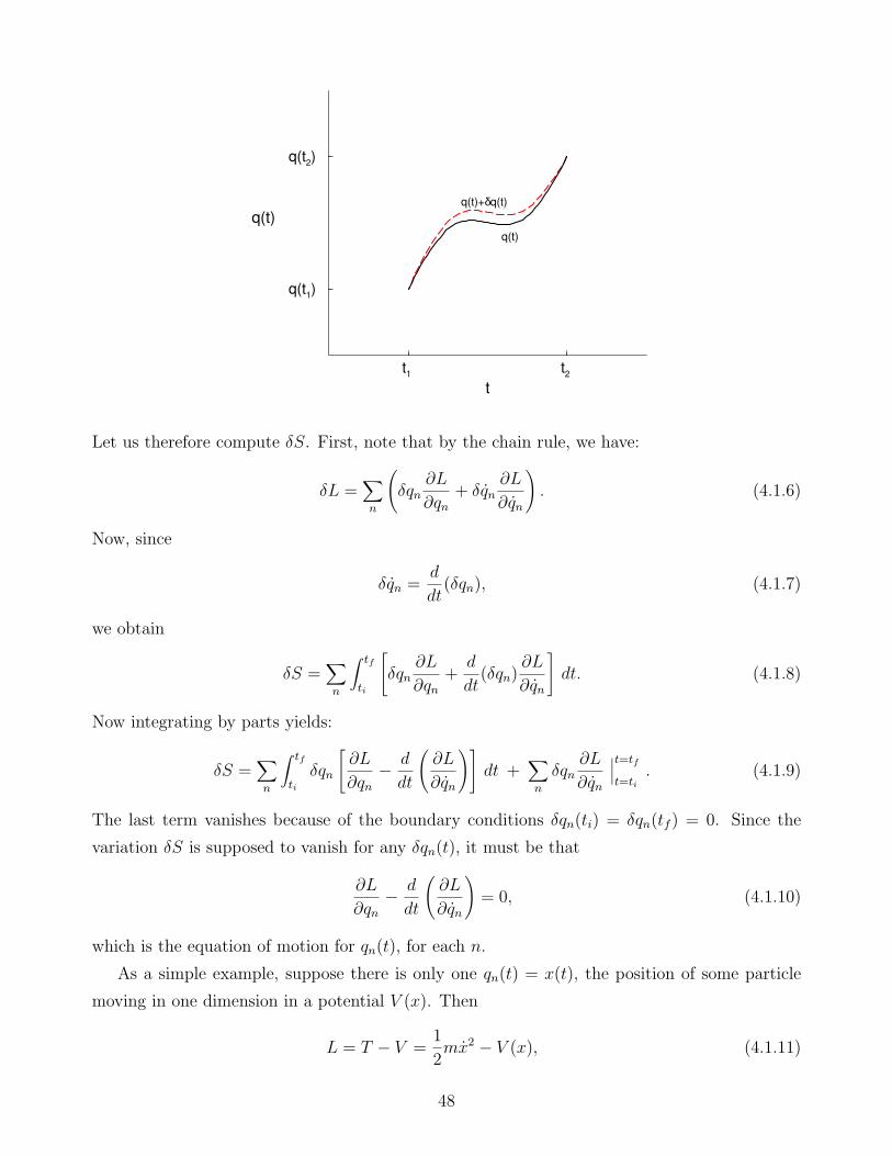
t1

t2

t

q(t1)

q(t2)

q(t)q(t)

q(t)+δq(t)

Let us therefore compute δS. First, note that by the chain rule, we have:

δL =∑

n

(δqn

∂L

∂qn+ δqn

∂L

∂qn

). (4.1.6)

Now, since

δqn =d

dt(δqn), (4.1.7)

we obtain

δS =∑

n

∫ tf

ti

[δqn

∂L

∂qn+d

dt(δqn)

∂L

∂qn

]dt. (4.1.8)

Now integrating by parts yields:

δS =∑

n

∫ tf

tiδqn

[∂L

∂qn− d

dt

(∂L

∂qn

)]dt +

∑

n

δqn∂L

∂qn

∣∣∣t=tf

t=ti. (4.1.9)

The last term vanishes because of the boundary conditions δqn(ti) = δqn(tf ) = 0. Since the

variation δS is supposed to vanish for any δqn(t), it must be that

∂L

∂qn− d

dt

(∂L

∂qn

)= 0, (4.1.10)

which is the equation of motion for qn(t), for each n.

As a simple example, suppose there is only one qn(t) = x(t), the position of some particle

moving in one dimension in a potential V (x). Then

L = T − V =1

2mx2 − V (x), (4.1.11)

48

from which there follows:

∂L

∂x= −∂V

∂x= F, (4.1.12)

which we recognize as the Newtonian force, and

d

dt

(∂L

∂x

)=

d

dt(mx) = mx. (4.1.13)

So the equation of motion is Newton’s second law:

F = mx. (4.1.14)

Everything we need to know about the dynamics of a physical system is encoded in the

action S, or equivalently the Lagrangian L. In quantum field theory, it will tell us what the

particle masses are, how they interact, how they decay, and what symmetries provide selection

rules on their behavior.

As a first example of an action for a relativistic field theory, consider a scalar field φ(x) =

φ(t, ~x). Then, in the previous discussion, we identify the label n with the spatial position ~x, and

qn(t) = φ(t, ~x). The action is obtained by summing contributions from each x:

S =∫ tf

tidt L(φ, φ) =

∫ tf

tidt∫d3~xL(φ, φ). (4.1.15)

Now, since this expression depends on φ, it must also depend on ~∇φ in order to be Lorentz

invariant. This just means that the form of the Lagrangian allows it to depend on the differences

between the field evaluated at infinitesimally nearby points. So, a better way to write the action

is:

S =∫d4xL(φ, ∂µφ). (4.1.16)

The object L is known as the Lagrangian density. Specifying a particular form for L defines the

theory.

To find the classical equations of motion for the field, we must find φ(x) so that S is extrem-

ized; in other words, for any small variation φ(x)→ φ(x) + δφ(x), we must have δS = 0. By a

similar argument as above, this implies the equations of motion:

δLδφ− ∂µ

(δL

δ(∂µφ)

)= 0. (4.1.17)

Here, we use δLδφ

to mean the partial derivative of L with respect to φ; δ is used rather than ∂

to avoid confusing between derivatives with respect to φ and spacetime partial derivatives with

49

respect to xµ. Likewise, δLδ(∂µφ)

means a partial derivative of L with respect to the object ∂µφ,

upon which it depends.

As an example, consider the choice:

L =1

2∂µφ∂

µφ− 1

2m2φ2. (4.1.18)

It follows that:

δLδφ

= −m2φ (4.1.19)

and

δLδ(∂µφ)

=δ

δ(∂µφ)

[1

2gαβ∂αφ∂βφ

]=

1

2gµβ∂βφ+

1

2gαµ∂αφ = ∂µφ. (4.1.20)

Therefore,

∂µ

(δL

δ(∂µφ)

)= ∂µ∂

µφ, (4.1.21)

and so the equation of motion following from eq. (4.1.17) is:

∂µ∂µφ+m2φ = 0. (4.1.22)

This we recognize as the Klein-Gordon wave equation for a scalar particle of mass m; compare

to eq. (3.1.13). This equation was originally introduced with the interpretation as the equation

governing the quantum wavefunction of a single scalar particle. Now it has reappeared with a

totally different interpretation, as the classical equation of motion for the scalar field.

The previous discussion for scalar fields can be extended to other types of fields as well.

Consider a general list of fields Φj(x), which could include scalar fields φ(x), Dirac or Majorana

fields Ψ(x) with four components, Weyl fields ψ(x) with two components, or vector fields Aµ(x)

with four components, or several copies of any of these. The Lagrangian density L(Φj, ∂µΦj)

determines the classical equations of motion through the principle that S =∫d4x L should

be stationary to first order when a deviation Φj(x) → Φj(x) + δΦj(x) is made, with boundary

conditions that δΦj(x) vanishes on the boundary of the spacetime region on which S is evaluated.

(Typically one evaluates S between two times ti and tf , and over all of space, so this means that

δΦ(x) vanishes very far away from some region of interest.) The Lagrangian density L should

be a real quantity that transforms under proper Lorentz transformations as a scalar.

Similarly to eq. (4.1.6), we have by the chain rule:

δS =∫d4x

∑

j

[δΦj

δLδΦj

+ δ(∂µΦj)

(δL

δ(∂µΦj)

)]. (4.1.23)

50

Now using δ(∂µΦj) = ∂µ(δΦj), and integrating the second term by parts (this is where the

boundary conditions come in), one obtains

δS =∫d4x

∑

j

δΦj

[δLδΦj

− ∂µ(

δLδ(∂µΦj)

)]. (4.1.24)

If we require this to vanish for each and every arbitrary variation δΦj, we obtain the Euler-

Lagrange equations of motion:

δLδΦj

− ∂µ(

δLδ(∂µΦj)

)= 0, (4.1.25)

for each j.

For example, let us consider how to make a Lagrangian density for a Dirac field Ψ(x). Under

Lorentz transformations, Ψ(x) transforms exactly like the wavefunction solution to the Dirac

equation. But now it is interpreted instead as a field; classically it is a function on spacetime, and

quantum mechanically it is an operator for each point xµ. Now, Ψ(x) is a complex 4-component

object, so Ψ†(x) is also a field. One should actually treat Ψ(x) and Ψ†(x) as independent fields,

in the same way that in complex analysis one often treats z = x + iy and z∗ = x − iy as

independent variables. As we found in section 3.1, if we want to build Lorentz scalar quantities,

it is useful to use Ψ(x) = Ψ†γ0 as a building block.

A good (and correct) guess for the Lagrangian for a Dirac field is:

L = iΨγµ∂µΨ−mΨΨ, (4.1.26)

which can also be written as:

L = iΨ†γ0γµ∂µΨ−mΨ†γ0Ψ. (4.1.27)

This is a Lorentz scalar, so that when integrated∫d4x it will give a Lorentz-invariant number.

Let us now compute the equations of motion that follow from it. First, let us find the equations

of motion obtained by varying with respect to Ψ†. For this, we need:

δLδΨ† = iγ0γµ∂µΨ−mγ0Ψ, (4.1.28)

δLδ(∂µΨ†)

= 0. (4.1.29)

The second equation just reflects the fact that the Lagrangian only contains the derivative of

Ψ, not the derivative of Ψ†. So, by plugging in to the general result eq. (4.1.25), the equation

of motion is simply:

iγµ∂µΨ−mΨ = 0, (4.1.30)

51

where we have multiplied δLδΨ† = 0 on the left by γ0 and used the fact that (γ0)2 = 1. This is, of

course, the Dirac equation.

We can also find the equations of motion obtained from the Lagrangian by varying with

respect to Ψ. For that, we need:

δLδΨ

= −mΨ, (4.1.31)

δLδ(∂µΨ)

= iΨγµ. (4.1.32)

Plugging these into eq. (4.1.25), we obtain:

−i∂µΨγµ −mΨ = 0. (4.1.33)

However, this is nothing new; it is just the Hermitian conjugate of eq. (4.1.30), multiplied on

the right by γ0 and using eq. (3.1.34).

The Lagrangian density for an electromagnetic field is:

LEM = −1

4FµνF

µν = −1

4(∂µAν − ∂νAµ)(∂

µAν − ∂νAµ). (4.1.34)

To find the equations of motion that follow from this Lagrangian, we compute:

δLEM

δAν

= 0, (4.1.35)

since Aµ doesn’t appear in the Lagrangian without a derivative acting on it, and

δLEM

δ(∂µAν)=

δ

δ(∂µAν)

[−1

4(∂αAβ − ∂βAα)(∂ρAσ − ∂σAρ)g

αρgβσ]

= −1

4

[(∂ρAσ − ∂σAρ)g

µρgνσ − (∂ρAσ − ∂σAρ)gνρgµσ

+(∂αAβ − ∂βAα)gµαgβσ − (∂αAβ − ∂αAβ)g

ναgµβ]

= −∂µAν + ∂νAµ

= −F µν . (4.1.36)

So, the equations of motion,

δLEM

δAν

− ∂µ(

δLEM

δ(∂µAν)

)= 0 (4.1.37)

reduce to

∂µFµν = 0, (4.1.38)

which we recognize as Maxwell’s equations in the case of vanishing Jµ [see eq. (2.4.13)]. In order

to include the effects of a 4-current Jµ, we can simply add a term

Lcurrent = −eJµAµ (4.1.39)

52

to the Lagrangian density. Then, since

δLcurrent

δAν

= −eJν ; (4.1.40)

δLcurrent

δ(∂µAν)= 0, (4.1.41)

the classical equations of motion for the vector field become

∂µFµν − eJν = 0, (4.1.42)

in agreement with eq. (2.4.13). The current density Jµ may be regarded as an external source

of unspecified origin for the electromagnetic field; or, it can be built out of the fields for charged

particles, as we will see.

4.2 Quantization of free scalar field theory

Let us now turn to the question of quantizing a field theory. To begin, let us recall how one

quantizes a simple generic system based on variables qn(t), given the Lagrangian L(qn, qn). First,

one defines the canonical momenta conjugate to each qn:

pn ≡∂L

∂qn. (4.2.1)

The classical Hamiltonian is then defined by

H(qn, pn) ≡∑

n

pnqn − L(qn, qn), (4.2.2)

where the qn are to be eliminated using eq. (4.2.1). To go to the corresponding quantum theory,

the qn and pn and H are reinterpreted as Hermitian operators acting on a Hilbert space of states.

The operators obey canonical equal-time commutation relations:

[pn, pm] = 0; (4.2.3)

[qn, qm] = 0; (4.2.4)

[pn, qm] = −ihδnm, (4.2.5)

and the time evolution of the system is determined by the Hamiltonian operator H.

Let us now apply this to the theory of a scalar field φ(x) with the Lagrangian density given

by eq. (4.1.18). Then φ(x) = φ(t, ~x) plays the role of qn(t), with ~x playing the role of the label

n; there is a different field at each point in space. The momentum conjugate to φ is:

π(~x) ≡ δLδφ

=δ

δφ

[12φ2 + . . .

]= φ. (4.2.6)

53

It should be emphasized that π(~x), the momentum conjugate to the field φ(~x), is not in any

way the mechanical momentum of the particle. Notice that π(~x) is a scalar function, not a

three-vector or a four-vector!

The Hamiltonian is obtained by summing over the fields at each point ~x:

H =∫d3~x π(~x)φ(x)− L (4.2.7)

=∫d3~x π(~x)φ(x)−

∫d3~x

1

2[φ2 − (~∇φ)2 −m2φ2] (4.2.8)

=1

2

∫d3~x [π2 + (~∇φ)2 +m2φ2]. (4.2.9)

Notice that a nice feature has emerged: this Hamiltonian is a sum of squares, and is therefore

always ≥ 0. There are no dangerous solutions with arbitrarily large negative energy, unlike the

case of the single-particle Klein-Gordon wave equation.

At any given fixed time t, the field operators φ(~x) and their conjugate momenta π(~x) are

Hermitian operators satisfying commutation relations exactly analogous to eqs. (4.2.3)-(4.2.5):

[φ(~x), φ(~y)] = 0; (4.2.10)

[π(~x), π(~y)] = 0; (4.2.11)

[π(~x), φ(~y)] = −ihδ(3)(~x− ~y). (4.2.12)

As we will see, it turns out to be profitable to analyze the system in a way similar to the way

one treats the harmonic oscillator in one-dimensional nonrelativistic quantum mechanics. In

that system, one defines “creation” and “annihilation” (or “raising” and “lowering”) operators

a† and a as complex linear combinations of the position and momentum operators x and p.

Similarly, here we will define:

a~p =∫d3~x e−i~p·~x [E~pφ(~x) + iπ(~x)] , (4.2.13)

where

E~p =√~p2 +m2, (4.2.14)

with the positive square root always taken. The overall coefficient in front of eq. (4.2.13) reflects

an arbitrary choice (and in fact it is chosen differently by various books). Equation (4.2.13)

defines a distinct annihilation operator for each three-momentum ~p. Taking the Hermitian

conjugate yields:

a†~p =∫d3~x ei~p·~x [E~pφ(~x)− iπ(~x)] . (4.2.15)

54

To see the usefulness of these definitions, compute the commutator:

[a~p, a†~k] =

∫d3~x

∫d3~y e−i~p·~xei

~k·~y [E~pφ(~x) + iπ(~x) , E~k φ(~y)− iπ(~y)] (4.2.16)

=∫d3~x

∫d3~y e−i~p·~xei

~k·~y (E~k + E~p) δ(3)(~x− ~y), (4.2.17)

where eqs. (4.2.10)-(4.2.12) have been used. Now performing the ~y integral using the definition

of the delta function, one obtains:

[a~p, a†~k] = (E~k + E~p)

∫d3~x ei(

~k−~p)·x . (4.2.18)

This can be further reduced by using the important identity:∫d3~x ei~q·~x = (2π)3δ(3)(~q ), (4.2.19)

valid for any 3-vector ~q, to obtain the final result:

[a~p, a†~k] = (2π)32E~p δ

(3)(~k − ~p). (4.2.20)

Here we have put E~k = E~p, using the fact that the delta function vanishes except when ~k = ~p.

In a similar way, one can check the commutators:

[a~p, a~k] = [a†~p, a†~k] = 0. (4.2.21)

Up to a constant factor on the right-hand side of eq. (4.2.20), these results have the same form

as the harmonic oscillator algebra familiar from non-relativistic quantum mechanics: [a, a†] = 1;

[a, a] = [a†, a†] = 0. Therefore, the quantum mechanics of a scalar field behaves like an infinite

collection of harmonic oscillators, one associated with each three-momentum ~p.

Now we can understand the Hilbert space of states for the quantum field theory. We start

with the vacuum state |0〉, which is taken to be annihilated by all of the lowering operators:

a~k|0〉 = 0. (4.2.22)

Acting on the vacuum state with any raising operator produces

a†~k|0〉 = |~k〉, (4.2.23)

which describes a state with a single particle with three-momentum ~k (and no definite position).

Acting multiple times with raising operators produces a state with multiple particles. So

a†~k1a†~k2

. . . a†~kn|0〉 = |~k1, ~k2, . . . , ~kn〉 (4.2.24)

describes a state of the universe with n φ-particles with momenta ~k1, ~k2, . . . , ~kn. Note that these

states are automatically symmetric under interchange of any two of the momentum labels ~ki,

55

because of the identity [a†~ki, a†~kj

] = 0. This is another way of saying that the multiparticle states

obey Bose-Einstein statistics for identical particles with integer (in this case, 0) spin.

In order to check our interpretation of the quantum theory, let us now evaluate the Hamil-

tonian operator in terms of the raising and lowering operators, and then determine how H acts

on the space of states. First, let us invert the definitions eqs. (4.2.13) and (4.2.15) to find φ(~x)

and π(~y) in terms of the a†~p and a~p. We begin by noting that:

a~p + a†−~p =∫d3~x e−i~p·~x2E~pφ(~x). (4.2.25)

Now we act on both sides by:∫dp ei~p·~y, (4.2.26)

where we have introduced the very convenient shorthand notation:

∫dp ≡

∫ d3~p

(2π)32E~p

, (4.2.27)

used often from now on. The result is that eq. (4.2.25) becomes

∫dp ei~p·~y(a~p + a†−~p) =

∫d3~x φ(~x)

∫ d3~p

(2π)3ei~p·(~y−~x)

. (4.2.28)

Since the ~p integral in braces is equal to δ(3)(~y−~x) [see eq. (4.2.19)], one obtains after performing

the ~x integral:

φ(~y) =∫dp ei~p·~y(a~p + a†−~p), (4.2.29)

or, renaming ~y → ~x, and ~p→ −~p in the second term on the right:

φ(~x) =∫dp (ei~p·~xa~p + e−i~p·~xa†~p). (4.2.30)

This expresses the original field in terms of raising and lowering operators. Similarly, for the

conjugate momentum field, one finds:

π(~x) = −i∫dp E~p (e

i~p·~xa~p − e−i~p·~xa†~p). (4.2.31)

Now we can plug the results of eqs. (4.2.30) and (4.2.31) into the expression eq. (4.2.9) for

the Hamiltonian. The needed terms are:

1

2

∫d3~x π(x)2 =

1

2

∫d3~x

∫dk∫dp (−i)2E~kE~p

(ei~k·~xa~k − e−i~k·~xa†~k

) (ei~p·~xa~p − e−i~p·~xa†~p

), (4.2.32)

1

2

∫d3~x (~∇φ)2 =

1

2

∫d3~x

∫dk∫dp

(i~kei

~k·~xa~k − i~ke−i~k·~xa†~k

)·(i~pei~p·~xa~p − i~pe−i~p·~xa†~p

), (4.2.33)

m2

2

∫d3~x φ(x)2 =

m2

2

∫d3~x

∫dk∫dp

(ei~k·~xa~k + e−i~k·~xa†~k

) (ei~p·~xa~p + e−i~p·~xa†~p

). (4.2.34)

56

Adding up the pieces, one finds:

H =1

2

∫dk∫dp∫d3~x

(m2 − ~k · ~p− E~kE~p)

[a~ka~p e

i(~k+~p)·~x + a†~ka†~p e

−i(~k+~p)·~x]

+(m2 + ~k · ~p+ E~kE~p)[a†~ka~p e

i(~p−~k)·~x + a~ka†~p e

i(~k−~p)·~x]

. (4.2.35)

Now one can do the ~x integration using:

∫d3~x e±i(~k+~p)·~x = (2π)3δ(3)(~k + ~p ), (4.2.36)

∫d3~x e±i(~k−~p)·~x = (2π)3δ(3)(~k − ~p ). (4.2.37)

As a result, the coefficient (m2−~k · ~p−E~kE~p) of the aa and a†a† terms vanishes after plugging

in ~k = −~p as enforced by the delta function. Meanwhile, for the aa† and a†a terms one has

~k = ~p from the delta function, so that

(m2 + ~k · ~p+ E~kE~p)δ(3)(~k − ~p) = 2E2

~p δ(3)(~k − ~p). (4.2.38)

Now performing the ~k integral in eq. (4.2.35), one finds:

H =1

2

∫dp E~p

(a†~p a~p + a~p a

†~p

). (4.2.39)

Finally, we can rearrange the second term, using

a~p a†~p = a†~p a~p + (2π)32E~p δ

(3)(~p− ~p) (4.2.40)

from eq. (4.2.20). The last term is infinite, so

H =∫dp E~p a

†~p a~p + ∞, (4.2.41)

where “∞” means an infinite, but constant, contribution to the energy. Since a uniform constant

contribution to the energy of all states is unobservable and commutes will all other operators, we

are free to drop it, by a redefinition of the Hamiltonian. This is a simple example of the process

known as renormalization. (In a more careful treatment, one could “regulate” the theory by

quantizing the theory confined to a box of finite volume, and neglecting all contributions coming

from momenta greater than some very large cutoff |~p|max. Then the infinite constant would be

rendered finite. Since we are going to ignore the constant anyway, we won’t bother doing this.)

So, from now on,

H =∫dp E~p a

†~p a~p (4.2.42)

is the Hamiltonian operator.

57

Acting on the vacuum state,

H|0〉 = 0, (4.2.43)

since all a~p annihilate the vacuum. This shows that the infinite constant we dropped from H

is actually the infinite energy density associated with an infinite universe of empty space, filled

with the zero-point energies of an infinite number of oscillators, one for each possible momentum

3-vector ~p. But we’ve already agreed to ignore it, so let it go. One can show that:

[H, a†~k] = E~k a†~k. (4.2.44)

Acting with H on a one-particle state, we therefore obtain

H|~k〉 = Ha†~k|0〉 = [H, a†~k]|0〉 = E~k a†~k|0〉 = E~k |~k〉. (4.2.45)

This proves that the one-particle state with 3-momentum ~k has energy eigenvalue E~k =√~k2 +m2,

as expected from special relativity. More generally, a multi-particle state

|~k1, ~k2, . . . , ~kn〉 = a†~k1a†~k2

. . . a†~kn|0〉 (4.2.46)

is easily shown to be an eigenstate of H with eigenvalue E~k1+ E~k2

+ . . . + E~kn. Note that it is

not possible to construct a state with a negative energy eigenvalue!

4.3 Quantization of free Dirac fermion field theory

Let us now apply the wisdom obtained by the quantization of a scalar field in the previous sub-

section to the problem of quantizing a Dirac fermion field that describes electrons and positrons.

A sensible strategy is to expand the fields Ψ and Ψ† in terms of operators that act on states by

creating and destroying particles with a given 3-momentum. Now, since Ψ is a spinor with four

components, one must expand it in a basis for the four-dimensional spinor space. A convenient

such basis is the solutions we found to the Dirac equation, u(p, s) and v(p, s). So we expand the

Dirac field, at a given fixed time t, as:

Ψ(~x) =2∑

s=1

∫dp

[u(p, s)ei~p·~xb~p,s + v(p, s)e−i~p·~xd†~p,s

]. (4.3.1)

Here s labels the two possible spin states in some appropriate basis (for example, Sz = ±1/2).The operator b~p,s will be interpreted as an annihilation operator, which removes an electron,

with 3-momentum ~p and spin state s, from whatever state it acts on. The operator d†~p,s is a

creation operator, which adds a positron to whatever state it acts on. We are using b, b† and d, d†

rather than a, a† in order to distinguish the fermion and antifermion creation and annihilation

58

operators from the scalar field versions. Taking the Hermitian conjugate of eq. (4.3.1), and

multiplying by γ0 on the right, we get:

Ψ(~x) =2∑

s=1

∫dp

[u(p, s)e−i~p·~xb†~p,s + v(p, s)ei~p·~xd~p,s

]. (4.3.2)

The operator b†~p,s creates an electron, and d~p,s destroys a positron, with the corresponding 3-

momentum and spin.

More generally, if the Dirac field describes some fermions other than the electron-positron

system, then you can substitute “particle” for electron and “antiparticle” for positron. So b†, b

act on states to create and destroy particles, while d†, d create and destroy antiparticles.

Just as in the case of a scalar field, we assume the existence of a vacuum state |0〉, whichdescribes a universe of empty space with no electrons or positrons present. The annihilation

operators yield 0 when acting on the vacuum state:

b~p,s|0〉 = d~p,s|0〉 = 0 (4.3.3)

for all ~p and s. To make a state describing a single electron with 3-momentum ~p and spin state

s, just act on the vacuum with the corresponding creation operator:

b†~p,s|0〉 = |e−~p,s〉. (4.3.4)

Similarly,

b†~k,rb†~p,s|0〉 = |e−~k,r; e

−~p,s〉 (4.3.5)

is a state containing two electrons, etc.

Now, electrons are fermions; they must obey Fermi-Dirac statistics for identical particles.

This means that if we interchange the momentum and spin labels for the two electrons in the

state of eq. (4.3.5), we must get a minus sign:

|e−~k,r; e−~p,s〉 = −|e−~p,s; e−~k,r〉. (4.3.6)

A corollary of this is the Pauli exclusion principle, which states that two electrons cannot be in

exactly the same state. In the present case, that means that we cannot add to the vacuum two

electrons with exactly the same 3-momentum and spin. Taking ~k = ~p and r = s in eq. (4.3.6):

|e−~p,s; e−~p,s〉 = −|e−~p,s; e−~p,s〉, (4.3.7)

which can only be true if |e−~p,s; e−~p,s〉 = 0, in other words there is no such state.

59

Writing eq. (4.3.6) in terms of creation operators, we have:

b†~k,rb†~p,s|0〉 = −b†~p,sb†~k,r|0〉. (4.3.8)

So, instead of the commutation relation

[b†~k,r, b†~p,s] = 0 (Wrong!) (4.3.9)

that one might expect from comparison with the scalar field, we must have an anticommutation

relation:

b†~k,rb†~p,s + b†~p,sb

†~k,r

= b†~k,r, b†~p,s = 0. (4.3.10)

Taking the Hermitian conjugate, we must also have:

b~k,r, b~p,s = 0. (4.3.11)

Similarly, applying the same thought process to identical positron fermions, one must have:

d†~k,r, d†~p,s = d~k,r, d~p,s = 0. (4.3.12)

Note that in the classical limit, h→ 0, these equations are unaffected, since h doesn’t appear

anywhere. So it must be true that b, b†, d, and d† anticommute even classically. So, as classical

fields, one must have

Ψ(x),Ψ(y) = 0, (4.3.13)

Ψ†(x),Ψ†(y) = 0, (4.3.14)

Ψ(x),Ψ†(y) = 0. (4.3.15)

Evidently, the classical Dirac field is not a normal number, but rather an anticommuting or

Grassmann number. Interchanging the order of any two Grassmann numbers results in an

overall minus sign.

In order to discover how the classical equations (4.3.13) and (4.3.15) are modified when one

goes to the quantum theory, let us construct the momentum conjugate to Ψ(~x). It is:

P(~x) = δLδ(∂0Ψ)

= iΨγ0 = iΨ†γ0γ0 = iΨ†. (4.3.16)

So the momentum conjugate to the Dirac spinor field is just i times its Hermitian conjugate.

Now, naively following the path of canonical quantization, one might expect the equal-time

commutation relation:

[P(~x),Ψ(~y )] = −ihδ(3)(~x− ~y ). (Wrong!) (4.3.17)

60

However, this clearly cannot be correct, since these are anticommuting fields; in the classical

limit h → 0, eq. (4.3.17) disagrees with eq. (4.3.15). So, instead we postulate a canonical

anticommutation relation for the Dirac field operator and its conjugate momentum operator:

P(~x), Ψ(~y ) = −ihδ(3)(~x− ~y ). (4.3.18)

Now just rewriting P = i؆, this becomes:

Ψ†(~x),Ψ(~y ) = −hδ(3)(~x− ~y ). (4.3.19)

From this, using a strategy similar to that used for scalar fields, one can obtain:

b~p,s, b†~k,r = d~p,s, d†~k,r = (2π)32E~p δ(3)(~p− ~k) δsr, (4.3.20)

and all other anticommutators of b, b†, d, d† operators vanish.

One also can check that the Hamiltonian is

H =2∑

s=1

∫dp E~p (b

†~p,sb~p,s + d†~p,sd~p,s) (4.3.21)

in a way very similar to the way we found the Hamiltonian for a scalar field in terms of a, a†

operators. In doing so, one must again drop an infinite constant contribution (negative, this

time) which is unobservable because it is the same for all states. Note that H again has energy

eigenvalues that are ≥ 0. One can show that:

[H, b†~k,s] = E~k b†~k,s, (4.3.22)

[H, d†~k,s] = E~k d†~k,s. (4.3.23)

(Note that these equations are commutators rather than anticommutators!) It follows that the

eigenstates of energy and 3-momentum are given in general by:

b†~p1,s1 . . . b†~pn,sn

d†~k1,r1. . . d†~km,rm

|0〉, (4.3.24)

which describes a state with n electrons (particles) and m positrons (antiparticles) with the

obvious 3-momenta and spins, and total energy E~p1 + . . .+ E~pn + E~k1+ . . .+ E~km

.

4.4 Scalar field with φ4 coupling

So far, we have been dealing with free field theories. These are theories in which the Lagrangian

density is quadratic in the fields, so that the Euler-Lagrange equations obtained by varying Lare linear wave equations in the fields, with exact solutions that are not too hard to find. At

the quantum level, this nice feature shows up in the simple time evolution of the states. In field

61

theory, as in any quantum system, the time evolution of a state |X〉 is given in the Schrodinger

picture by

ihd

dt|X〉 = H|X〉. (4.4.1)

So, in the case of a multiparticle state with an energy eigenvalue E as described above, the

solution is just

|X(t)〉 = e−i(t−t0)H |X(t0)〉 = e−i(t−t0)E|X(t0)〉. (4.4.2)

In other words, the state at some time t is just the same as the state at some previous time t0,

up to a phase. So nothing ever happens to the particles in a free theory; their number does not

change, and their momenta and spins remain the same.

We are interested in describing a more interesting situation where particles can scatter off

each other, perhaps inelastically to create new particles, and in which some particles can decay

into other sets of particles. To describe this, we need a Lagrangian density that contains terms

with more than two fields. At the classical level, this will lead to non-linear equations of motion

that have to be solved approximately. At the quantum level, finding exact energy eigenstates of

the Hamiltonian is not possible, so one usually treats the non-quadratic part of the Hamiltonian

as a perturbation on the quadratic part, giving an approximate answer.

As an example, consider the free Lagrangian for a scalar field φ, as given in eq. (4.1.18), and

add to it an interaction term:

L = L0 + Lint; (4.4.3)

Lint = − λ

24φ4. (4.4.4)

Here λ is a dimensionless number, a parameter of the theory known as a coupling. It governs

the strength of interactions; if we set λ = 0, we would be back to the free theory in which

nothing interesting ever happens. The factor of 1/4! = 1/24 is a convention, and the reason for

it will be apparent later. Now canonical quantization can proceed as before, except that now

the Hamiltonian is

H = H0 +Hint, (4.4.5)

where

Hint = −∫d3~x Lint =

λ

24

∫d3~x φ(~x)4. (4.4.6)

Let us write this in terms of creation and annihilation operators, using eq. (4.2.30):

Hint =λ

24

∫d3~x

∫dq1

∫dq2

∫dq3

∫dq4

(a~q1e

i~q1·~x + a†~q1e−i~q1·~x

) (a~q2e

i~q2·~x + a†~q2e−i~q2·~x

)

(a~q3e

i~q3·~x + a†~q3e−i~q3·~x

) (a~q4e

i~q4·~x + a†~q4e−i~q4·~x

). (4.4.7)

62

Now we can perform the d3~x integration, using eq. (4.2.19). The result is:

Hint =λ

24(2π)3

∫dq1

∫dq2

∫dq3

∫dq4

[a†~q1a

†~q2a†~q3a

†~q4δ(3)(~q1 + ~q2 + ~q3 + ~q4)

+4a†~q1a†~q3a†~q3a~q4 δ

(3)(~q1 + ~q2 + ~q3 − ~q4)+6a†~q1a

†~q2a~q3a~q4 δ

(3)(~q1 + ~q2 − ~q3 − ~q4)+4a†~q1a~q2a~q3a~q4 δ

(3)(~q1 − ~q3 − ~q3 − ~q4)

+a~q1a~q2a~q3a~q4 δ(3)(~q1 + ~q2 + ~q3 + ~q4)

]. (4.4.8)

Here we have combined several like terms, by relabeling the momenta, giving rise to the factors

of 4, 6, and 4. This involves reordering the a’s and a†’s. In doing so, we have ignored the fact

that a’s do not commute with a†’s when the 3-momenta are exactly equal. This should not cause

any worry, because it just corresponds to the situation where a particle is “scattered” without

changing its momentum at all, which is the same as no scattering, and therefore not of interest.

To see how to use the interaction Hamiltonian, it is useful to tackle a specific process. For

example, consider a scattering problem in which we have two scalar particles with 4-momenta

pa, pb that interact, producing two scalar particles with 4-momenta k1, k2:

papb → k1k2. (4.4.9)

We will work in the Schrodinger picture of quantum mechanics, in which operators are time-

independent and states evolve in time according to eq. (4.4.1). Nevertheless, in the far past, we

assume that the incoming particles were far apart, so the system is accurately described by the

free Hamiltonian and its energy eigenstates. The same applies to the outgoing particles in the

far future. So, we can pretend that Hint is “turned off” in both the far past and the far future.

The states that are simple two-particle states are

|pa, pb〉IN = a†~paa†~pb|0〉, (4.4.10)

in the far past, and

|k1, k2〉OUT = a†~k1a†~k2|0〉, (4.4.11)

in the far future. These are built out of creation and annihilation operators just as before, so

they are eigenstates of the free Hamiltonian H0, but not of the full Hamiltonian. Now, we are

interested in computing the probability amplitude that the state |pa, pb〉IN evolves to the state

|k1, k2〉OUT. According to the rules of quantum mechanics this is given by their overlap at a

common time, say in the far future:

OUT〈k1, k2|pa, pb〉OUT. (4.4.12)

63

The state |pa, pb〉OUT is the time evolution of |pa, pb〉IN from the far past to the far future:

|pa, pb〉OUT = e−iTH |pa, pb〉IN, (4.4.13)

where T is the long time between the far past time when the initial state was created and the

far future time at which the overlap is computed. So we have:

OUT〈k1, k2|pa, pb〉OUT = OUT〈k1, k2|e−iTH |pa, pb〉IN. (4.4.14)

The states appearing on the right-hand side are simple; see eqs. (4.4.10) and (4.4.11). The

complications are hidden in the operator e−iTH .

In general, e−iTH cannot be written exactly in a useful way in terms of creation and anni-

hilation operators. However, we can do it perturbatively, order by order in the coupling λ. For

example, let us consider the contribution linear in λ. We use the definition of the exponential

to write:

e−iTH = [1− iHT/N ]N = [1− i(H0 +Hint)T/N ]N , (4.4.15)

for N →∞. Now, the part of this that is linear in Hint can be expanded as:

e−iTH =N−1∑

n=0

[1− iH0T/N ]N−n−1 (−iHintT/N) [1− iH0T/N ]n . (4.4.16)

(Here we have dropped the 0th order part, e−iTH0 , as uninteresting; it just corresponds to the

particles evolving as free particles.) We can now turn this discrete sum into an integral, by

letting t = nT/N and dt = T/N in the limit of large N :

e−iTH = −i∫ T

0dt e−i(T−t)H0Hinte

−itH0 . (4.4.17)

Next we can use the fact that we know whatH0 is when acting on the simple states of eqs. (4.4.10)

and (4.4.11):

e−itH0|pa, pb〉IN = e−itEi |pa, pb〉IN, (4.4.18)

OUT〈k1, k2|e−i(T−t)H0 = OUT〈k1, k2|e−i(T−t)Ef , (4.4.19)

where

Ei = E~pa + E~pb , Ef = E~k1+ E~k2

(4.4.20)

are the energies of the initial and final states, respectively. So we have:

OUT〈k1, k2|e−iTH |pa, pb〉IN = −i∫ T

0dt e−i(T−t)Ef e−itEi

OUT〈k1, k2|Hint|pa, pb〉IN. (4.4.21)

64

First let us do the t integral:

∫ T

0dt e−i(T−t)Ef e−itEi = e−i(Ef+Ei)T/2

∫ T/2

−T/2dt′ eit

′(Ef−Ei) (4.4.22)

where we have redefined the integration variable by t = t′ + T/2. As we take T → ∞, we can

use the integral identity

∫ ∞

−∞dx eixA = 2πδ(A) (4.4.23)

to obtain:

∫ T

0dt e−i(T−t)Ef e−itEi = 2π δ(Ef − Ei) e

−i(Ef+Ei)T/2. (4.4.24)

This tells us that energy conservation will be enforced, and (dropping the phase factor e−i(Ef+Ei)T/2,

which will just give 1 when we take the complex square of the probability amplitude):

OUT〈k1, k2|pa, pb〉OUT = −i 2π δ(Ef − Ei) OUT〈k1, k2|Hint|pa, pb〉IN. (4.4.25)

Now we are ready to use our expression for Hint in eq. (4.4.8). The action of Hint on

eigenstates of the free Hamiltonian can be read off from the different types of terms. The

aaaa-type term will remove four particles from the state. Clearly we don’t have to worry about

that, because there were only two particles in the state to begin with! The same goes for the

a†aaa-type term. The terms of type a†a†a†a† and a†a†a†a create more than the two particles

we know to be in the final state, so we can ignore them too. Therefore, the only term that will

play a role in this example is the a†a†aa contribution:

Hint =λ

4(2π)3

∫dq1

∫dq2

∫dq3

∫dq4 δ

(3)(~q1 + ~q2 − ~q3 − ~q4) a†~q1a†~q2a~q3a~q4 , (4.4.26)

Therefore, we have:

OUT〈k1, k2|pa, pb〉OUT = −i(2π)4λ4

∫dq1

∫dq2

∫dq3

∫dq4 δ

(4)(q1 + q2 − q3 − q4)

OUT〈k1, k2|a†~q1a†~q2a~q3a~q4|pa, pb〉IN. (4.4.27)

Here we have combined the three-momenta delta function from eq. (4.4.26) with the energy

delta function from eq. (4.4.25) to give a 4-momentum delta function.

It remains to evaluate:

OUT〈k1, k2|a†~q1a†~q2a~q3a~q4 |pa, pb〉IN, (4.4.28)

which, according to eqs. (4.4.10) and (4.4.11), is equal to

〈0|a~k1a~k2a†~q1a†~q2a~q3a~q4a

†~paa†~pb |0〉. (4.4.29)

65

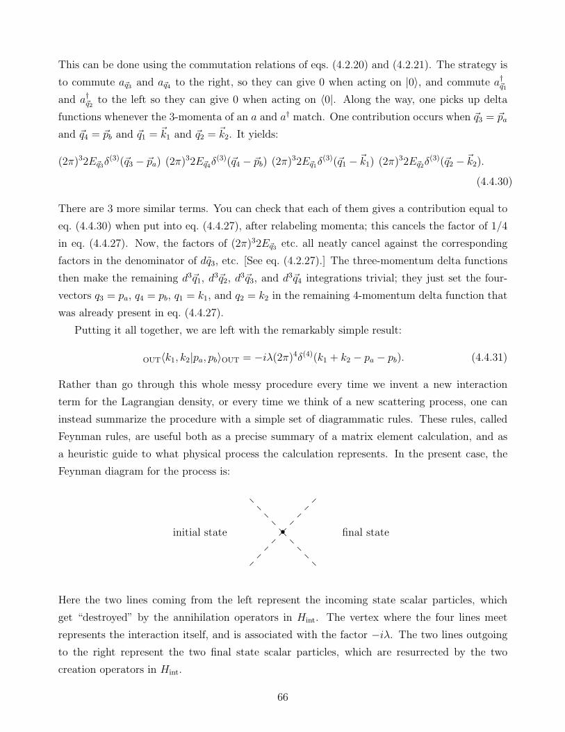
This can be done using the commutation relations of eqs. (4.2.20) and (4.2.21). The strategy is

to commute a~q3 and a~q4 to the right, so they can give 0 when acting on |0〉, and commute a†~q1and a†~q2 to the left so they can give 0 when acting on 〈0|. Along the way, one picks up delta

functions whenever the 3-momenta of an a and a† match. One contribution occurs when ~q3 = ~pa

and ~q4 = ~pb and ~q1 = ~k1 and ~q2 = ~k2. It yields:

(2π)32E~q3δ(3)(~q3 − ~pa) (2π)32E~q4δ

(3)(~q4 − ~pb) (2π)32E~q1δ(3)(~q1 − ~k1) (2π)32E~q2δ

(3)(~q2 − ~k2).(4.4.30)

There are 3 more similar terms. You can check that each of them gives a contribution equal to

eq. (4.4.30) when put into eq. (4.4.27), after relabeling momenta; this cancels the factor of 1/4

in eq. (4.4.27). Now, the factors of (2π)32E~q3 etc. all neatly cancel against the corresponding

factors in the denominator of dq3, etc. [See eq. (4.2.27).] The three-momentum delta functions

then make the remaining d3~q1, d3~q2, d

3~q3, and d3~q4 integrations trivial; they just set the four-

vectors q3 = pa, q4 = pb, q1 = k1, and q2 = k2 in the remaining 4-momentum delta function that

was already present in eq. (4.4.27).

Putting it all together, we are left with the remarkably simple result:

OUT〈k1, k2|pa, pb〉OUT = −iλ(2π)4δ(4)(k1 + k2 − pa − pb). (4.4.31)

Rather than go through this whole messy procedure every time we invent a new interaction

term for the Lagrangian density, or every time we think of a new scattering process, one can

instead summarize the procedure with a simple set of diagrammatic rules. These rules, called

Feynman rules, are useful both as a precise summary of a matrix element calculation, and as

a heuristic guide to what physical process the calculation represents. In the present case, the

Feynman diagram for the process is:

initial state final state

Here the two lines coming from the left represent the incoming state scalar particles, which

get “destroyed” by the annihilation operators in Hint. The vertex where the four lines meet

represents the interaction itself, and is associated with the factor −iλ. The two lines outgoing

to the right represent the two final state scalar particles, which are resurrected by the two

creation operators in Hint.

66

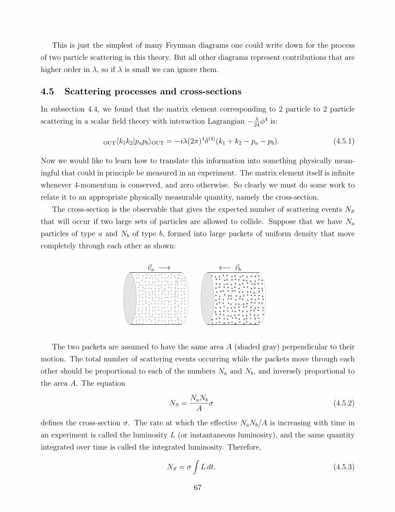
This is just the simplest of many Feynman diagrams one could write down for the process

of two particle scattering in this theory. But all other diagrams represent contributions that are

higher order in λ, so if λ is small we can ignore them.

4.5 Scattering processes and cross-sections

In subsection 4.4, we found that the matrix element corresponding to 2 particle to 2 particle

scattering in a scalar field theory with interaction Lagrangian − λ24φ4 is:

OUT〈k1k2|papb〉OUT = −iλ(2π)4δ(4)(k1 + k2 − pa − pb). (4.5.1)

Now we would like to learn how to translate this information into something physically mean-

ingful that could in principle be measured in an experiment. The matrix element itself is infinite

whenever 4-momentum is conserved, and zero otherwise. So clearly we must do some work to

relate it to an appropriate physically measurable quantity, namely the cross-section.

The cross-section is the observable that gives the expected number of scattering events NS

that will occur if two large sets of particles are allowed to collide. Suppose that we have Na

particles of type a and Nb of type b, formed into large packets of uniform density that move

completely through each other as shown:

~va −→ ←− ~vb

The two packets are assumed to have the same area A (shaded gray) perpendicular to their

motion. The total number of scattering events occurring while the packets move through each

other should be proportional to each of the numbers Na and Nb, and inversely proportional to

the area A. The equation

NS =NaNb

Aσ (4.5.2)

defines the cross-section σ. The rate at which the effective NaNb/A is increasing with time in

an experiment is called the luminosity L (or instantaneous luminosity), and the same quantity

integrated over time is called the integrated luminosity. Therefore,

NS = σ∫Ldt. (4.5.3)

67

The dimensions for cross-section are the same as area, and the official unit is 1 barn = 10−24

cm2 = 2568 GeV−2. However, from the point of view of modern high-energy experiments, a barn

is a very large cross-section,† so more commonly-used units are obtained by using the prefixes

nano-, pico-, and femto-:

1 nb = 10−33 cm2 = 2.568× 10−6 GeV−2, (4.5.4)

1 pb = 10−36 cm2 = 2.568× 10−9 GeV−2, (4.5.5)

1 fb = 10−39 cm2 = 2.568× 10−12 GeV−2. (4.5.6)

As an example, the Tevatron collided protons (p) and antiprotons (p) with a center-of-momentum

(CM) energy of ECM = 1960 GeV and each experiment received a total integrated luminosity of

about

∫Ldt = 12 fb−1 = 12, 000 pb−1, (4.5.7)

although not all of that data is useable in any given analysis. The Large Hadron Collider

(LHC) at CERN is a pp machine that previously collected 23.3 fb−1 of integrated luminosity

per experiment (ATLAS and CMS) at center-of-mass energy√s = 8TeV. The LHC has been

running at√s = 13TeV since 2015, with the goal of reaching several hundred fb−1 of integrated

luminosity in the coming years. As of this writing (August 2018), about 130 fb−1 have already

been delivered to each LHC experiment at√s = 13TeV, with the record highest luminosity in a

single day being about 860 pb−1. The highest instantaneous luminosity so far is about 2.1×1034

cm−2 sec−1, exceeding the LHC design target.

To figure out how many scattering events one expects at a collider, one needs to know the

corresponding cross-section for that type of event, which depends on the final state. The total

cross-section for any type of scattering at hadron colliders is quite large. By one estimate at the

Tevatron it was approximately

σ(pp→ anything) = 0.075 barns. (4.5.8)

However, this estimate is quite fuzzy, because it depends on detection variables such as the

minimum momentum transfer that one requires in order to say that a scattering event has

occurred. For arbitrarily small momentum transfer in elastic scattering of charged particles, the

cross-section actually becomes arbitrarily large due to the long-range nature of the Coulomb

force, as we will see in section 5.2.4. Also, the vast majority of the scattering events reflected in

eq. (4.5.8) are extremely uninteresting, featuring final states of well-known and well-understood

hadrons.

†The joke is that achieving an event with such a cross-section is “as easy as hitting the broad side of a barn”.

68

An example of a more interesting final state would be anything involving a top quark (t)and

anti-top quark (t) pair, for which the Tevatron cross-section was about

σ(pp→ tt+ anything) = 7.5 pb. (4.5.9)

This means that about 96,000 top pairs were produced at the Tevatron. However, only a small

fraction of these were identified as such. At the LHC, the cross-section for producing top-antitop

pairs is about

σ(pp→ tt+ anything) = (175, 250, 830) pb, (4.5.10)

for center-of-mass energies√s = (7, 8, 13) TeV, respectively. This means that tens of millions

of tt pairs have already been produced, enabling unprecedented precision studies of top quark

properties. Those studies will continue as the integrated luminosity increases.

A propaganda plot summarizing the theoretical predictions and experimental measurements

of cross-sections for a selection of some of the more important processes involving Standard

Model particles is shown on the next page for LHC energies of 7, 8, and 13 TeV. Besides the

very large total and the inelastic total, also shown are the cross-sections for producing ≥ 1 or

≥ 2 hadronic jets, a photon, a W boson, a Z boson, tt pairs, a single top quark, combinations

of vector bosons WW , WZ, ZZ, and γγ, the Higgs boson, and other even rarer processes as

labeled. In some cases, the cross-sections are given independently for sub-cases in which at least

a certain number of hadronic jets nj is required in the final state. Note that the ranges for

these cross-sections span many orders of magnitude. The plot shows both experimental results

and theoretical predictions for these cross-section. It is both gratifying and reassuring that

the theoretical predictions of the Standard Model are in good agreement with the experimental

results.

69

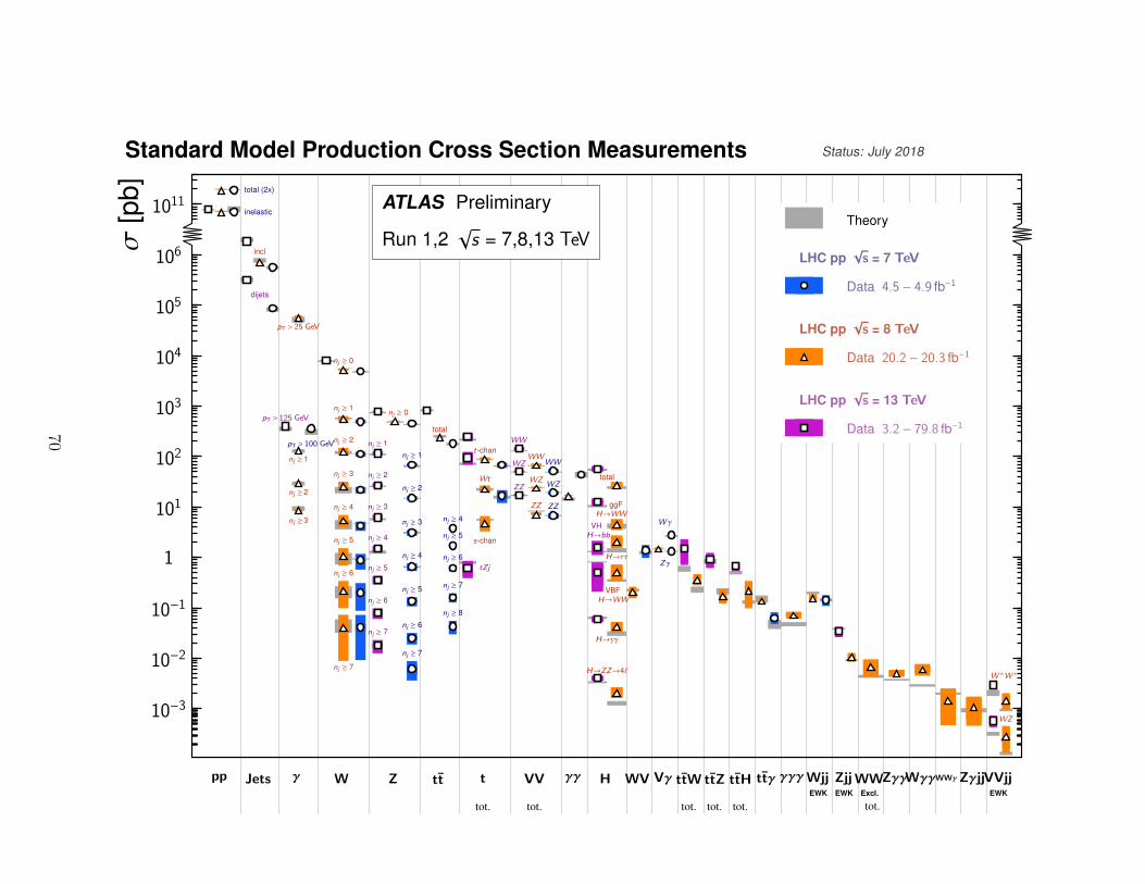
pp

total (2x)

inelastic

Jets

dijets

incl

γ

pT > 125 GeV

nj ≥ 3

pT > 25 GeV

nj ≥ 1

nj ≥ 2

pT > 100 GeV

W

nj ≥ 2

nj ≥ 3

nj ≥ 5

nj ≥ 1

nj ≥ 6

nj ≥ 7

nj ≥ 4

nj ≥ 0

Z

nj ≥ 7

nj ≥ 6

nj ≥ 4

nj ≥ 3

nj ≥ 2

nj ≥ 1

nj ≥ 5

nj ≥ 0

nj ≥ 7

nj ≥ 6

nj ≥ 4

nj ≥ 3

nj ≥ 2

nj ≥ 1

nj ≥ 5

tt

total

nj ≥ 6

nj ≥ 5

nj ≥ 4

nj ≥ 7

nj ≥ 8

t

tot.

tZj

Wt

t-chan

s-chan

VV

tot.

WW

WZ

ZZ

WW

WZ

ZZ

WW

WZ

ZZ

γγ H

VH

H→bb

total

ggF

H→WW

H→ZZ→4ℓ

VBF

H→WW

H→γγ

H→ττ

WV Vγ

Zγ

W γ

ttW

tot.

ttZ

tot.

ttH

tot.

ttγ γγγWjjEWK

ZjjEWK

WWExcl.

tot.

ZγγWγγWWγZγjjVVjjEWK

W ±W ±

WZ10−3

10−2

10−1

1

101

102

103

104

105

106

1011

σ[p

b]

Status: July 2018

ATLAS Preliminary

Run 1,2√s = 7,8,13 TeV

Theory

LHC pp√

s = 7 TeV

Data 4.5 − 4.9 fb−1

LHC pp√

s = 8 TeV

Data 20.2 − 20.3 fb−1

LHC pp√

s = 13 TeV

Data 3.2 − 79.8 fb−1

Standard Model Production Cross Section Measurements

70

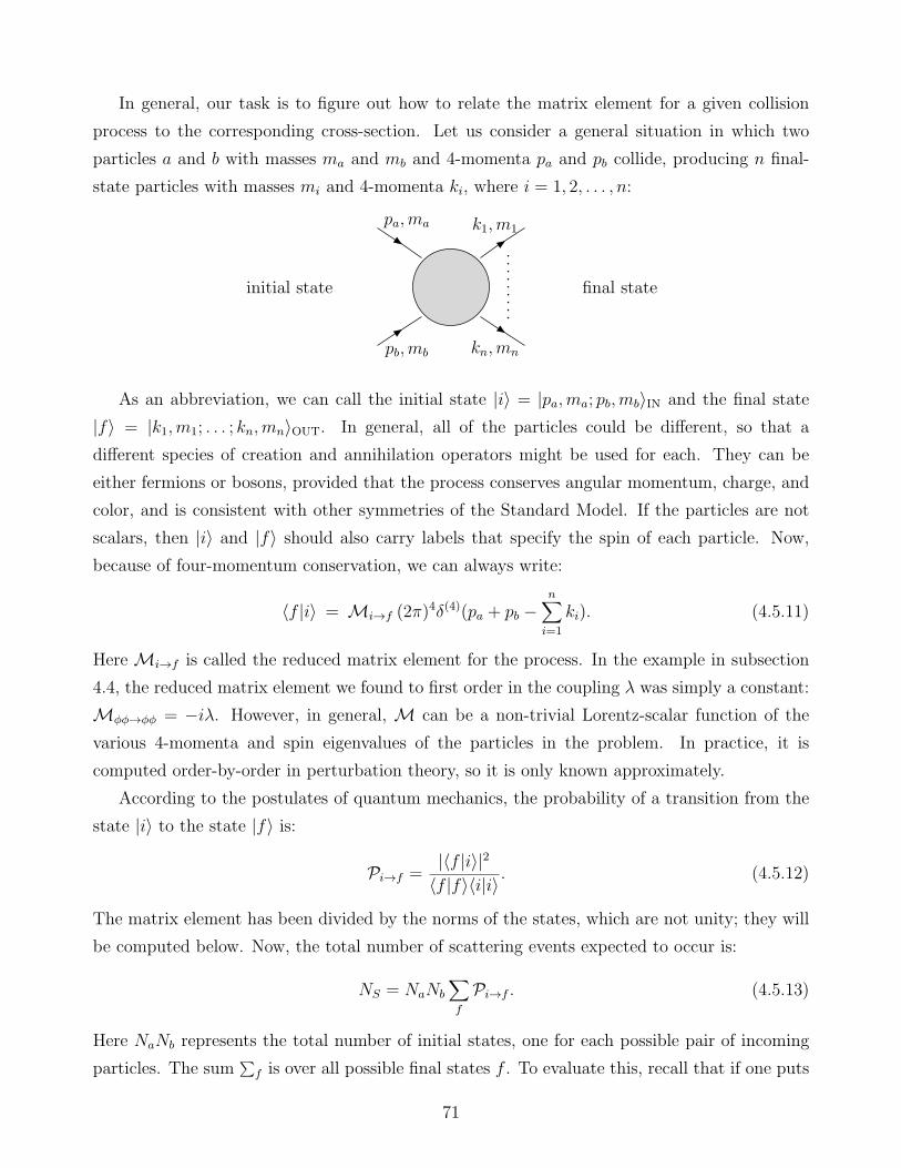
In general, our task is to figure out how to relate the matrix element for a given collision

process to the corresponding cross-section. Let us consider a general situation in which two

particles a and b with masses ma and mb and 4-momenta pa and pb collide, producing n final-

state particles with masses mi and 4-momenta ki, where i = 1, 2, . . . , n:

initial state final state

.........

pa,ma

pb,mb

k1,m1

kn,mn

As an abbreviation, we can call the initial state |i〉 = |pa,ma; pb,mb〉IN and the final state

|f〉 = |k1,m1; . . . ; kn,mn〉OUT. In general, all of the particles could be different, so that a

different species of creation and annihilation operators might be used for each. They can be

either fermions or bosons, provided that the process conserves angular momentum, charge, and

color, and is consistent with other symmetries of the Standard Model. If the particles are not

scalars, then |i〉 and |f〉 should also carry labels that specify the spin of each particle. Now,

because of four-momentum conservation, we can always write:

〈f |i〉 = Mi→f (2π)4δ(4)(pa + pb −

n∑

i=1

ki). (4.5.11)

HereMi→f is called the reduced matrix element for the process. In the example in subsection

4.4, the reduced matrix element we found to first order in the coupling λ was simply a constant:

Mφφ→φφ = −iλ. However, in general, M can be a non-trivial Lorentz-scalar function of the

various 4-momenta and spin eigenvalues of the particles in the problem. In practice, it is

computed order-by-order in perturbation theory, so it is only known approximately.

According to the postulates of quantum mechanics, the probability of a transition from the

state |i〉 to the state |f〉 is:

Pi→f =|〈f |i〉|2〈f |f〉〈i|i〉 . (4.5.12)

The matrix element has been divided by the norms of the states, which are not unity; they will

be computed below. Now, the total number of scattering events expected to occur is:

NS = NaNb

∑

f

Pi→f . (4.5.13)

Here NaNb represents the total number of initial states, one for each possible pair of incoming

particles. The sum∑

f is over all possible final states f . To evaluate this, recall that if one puts

71

particles in a large box of volume V , then the density of one-particle states with 3-momentum

~k is

density of states = Vd3~k

(2π)3. (4.5.14)

So, including a sum over the n final-state particles implies

∑

f

→n∏

i=1

V

∫ d3~ki(2π)3

. (4.5.15)

Putting this into eq. (4.5.13) and comparing with the definition eq. (4.5.2), we have for the

differential contribution to the total cross-section:

dσ = Pi→fAn∏

i=1

V

d3~ki(2π)3

. (4.5.16)

Let us now suppose that each packet of particles consists of a cylinder with a large volume

V . Then the total time T over which the particles can collide is given by the time it takes for

the two packets to move through each other:

T =V

A|~va − ~vb|. (4.5.17)

(Assume that the volume V and area A of each bunch are very large compared to the cube and

square of the particles’ Compton wavelengths.) It follows that the differential contribution to

the cross-section is:

dσ = Pi→fV

T |~va − ~vb|n∏

i=1

V

d3~ki(2π)3

. (4.5.18)

The total cross-section is obtained by integrating over 3-momenta of the final state particles.

Note that the differential cross-section dσ depends only on the collision process being studied.

So in the following we expect that the arbitrary volume V and packet collision time T should

cancel out.

To see how that happens in the example of φφ → φφ scattering with a φ4 interaction, let

us first compute the normalizations of the states appearing in Pi→f . For the initial state |i〉 ofeq. (4.4.10), one has:

〈i|i〉 = 〈0|a~pba~paa†~paa†~pb|0〉. (4.5.19)

To compute this, one can commute the a† operators to the left:

〈i|i〉 = 〈0|a~pb [a~paa†~pa ]a†~pb|0〉+ 〈0|a~pba†~paa~paa

†~pb|0〉. (4.5.20)

72

Now the incoming particle momenta ~pa and ~pb are always different, so in the last term the a†~pajust commutes with a~pb according to eq. (4.2.20), yielding 0 when acting on 〈0|. The first term

can be simplified using the commutator eq. (4.2.20):

〈i|i〉 = 〈0|a~pba†~pb |0〉 (2π)3 2Eaδ

(3)(~pa − ~pa). (4.5.21)

Commuting a†~pb to the left in the same way yields the norm of the state |i〉:

〈i|i〉 = (2π)6 4EaEb δ(3)(~pa − ~pa)δ(3)(~pb − ~pb). (4.5.22)

This result is doubly infinite, since the arguments of each delta function vanish! In order to

successfully interpret it, let us recall the origin of the 3-momentum delta functions. One can

write

(2π)3δ(3)(~p− ~p ) =∫d3~x ei

~0·~x = V, (4.5.23)

showing that a 3-momentum delta-function with vanishing argument corresponds to V/(2π)3,

where V is the volume that the particles occupy. So we obtain

〈i|i〉 = 4EaEbV2 (4.5.24)

for the norm of the incoming state.

Similarly, the norm of the state |f〉 is:

〈f |f〉 =n∏

i=1

(2π)32Eiδ(3)(~ki − ~ki) =

n∏

i=1

(2EiV ). (4.5.25)

In doing this, there is one subtlety; unlike the colliding particles, it could be that two identical

outgoing particles have exactly the same momentum. This seemingly could produce “extra”

contributions when we commute a† operators to the left. However, at least for massive particles,

one can usually ignore this, since the probability that two outgoing particles will have exactly

the same momentum is vanishingly small in the limit V →∞.

Next we turn to the square of the matrix element:

|〈f |i〉|2 = |Mi→f |2[(2π)4δ(4)(pa + pb −

∑ki)]2. (4.5.26)

This also is apparently the square of an infinite quantity. To interpret it, we again recall the

origin of the delta functions:

2πδ(Ef − Ei) =∫ T/2

−T/2dt eit(Ef−Ei) = T (for Ef = Ei), (4.5.27)

(2π)3δ(∑

~k −∑

~p ) =∫d3~x ei~x·(

∑~k−∑

~p ) = V (for∑

~k =∑

~p ). (4.5.28)

73

So we can write:

(2π)4δ(4)(pa + pb −n∑

i=1

ki) = TV. (4.5.29)

Now if we use this to replace one of the two 4-momentum delta functions in eq. (4.5.26), we

have:

|〈f |i〉|2 = |Mi→f |2 (2π)4 T V δ(4)(pa + pb −n∑

i=1

ki). (4.5.30)

Plugging the results of eqs. (4.5.24), (4.5.25) and (4.5.30) into eq. (4.5.12), we obtain an

expression for the transition probability:

Pi→f = |Mi→f |2 (2π)4δ(4)(pa + pb −n∑

i=1

ki)T

4EaEbV

n∏

i=1

(1

2EiV

). (4.5.31)

Putting this in turn into eq. (4.5.18), we finally obtain:

dσ =|Mi→f |2

4EaEb|~va − ~vb|dΦn, (4.5.32)

where dΦn is a short-hand notation for

dΦn = (2π)4δ(4)(pa + pb −n∑

i=1

ki)n∏

i=1

d3~ki(2π)32Ei

, (4.5.33)

and is known as the n-body differential Lorentz-invariant phase space: As expected, all factors

of T and V have canceled out of the formula eq. (4.5.32) for the differential cross-section.

In the formula eq. (4.5.32), one can write for the velocities:

~va =~paEa

, ~vb =~pbEb

. (4.5.34)

Now, assuming that the collision is head-on so that ~vb is opposite to ~va (or 0), the denominator

in eq. (4.5.32) is:

4EaEb|~va − ~vb| = 4(Ea|~pb|+ Eb|~pa|). (4.5.35)

The most common case one encounters is two-particle scattering to a final state with two

particles. In the center-of-momentum frame, ~pb = −~pa, so that the 2-body Lorentz-invariant

phase space becomes:

dΦ2 = (2π)4δ(3)(~k1 + ~k2)δ(Ea + Eb − E1 − E2)d3~k1

(2π)32E1

d3~k2(2π)32E2

(4.5.36)

=δ(3)(~k1 + ~k2) δ(

√~k21 +m2

1 +√~k22 +m2

2 − ECM)

16π2

√~k21 +m2

1

√~k22 +m2

2

d3~k1 d3~k2, (4.5.37)

74

where

ECM ≡ Ea + Eb (4.5.38)

is the center-of-momentum energy of the process. Now one can do the ~k2 integral; the 3-

momentum delta function just sets ~k2 = −~k1 (as it must be in the CM frame). If we define

K ≡ |~k1| (4.5.39)

for convenience, then

d3~k1 = K2dK dΩ = K2dK dφ d(cos θ), (4.5.40)

where Ω = (θ, φ) are the spherical coordinate angles for ~k1. So

∫. . . dΦ2 =

∫. . .

δ(√K2 +m2

1 +√K2 +m2

2 − ECM)√K2 +m2

1

√K2 +m2

2

K2dK dφ d(cos θ), (4.5.41)

where . . . represents any quantity. To do the remaining dK integral, it is convenient to change

variables to the argument of the delta function. So, defining

W =√K2 +m2

1 +√K2 +m2

2 − ECM, (4.5.42)

we find

dW =

√K2 +m2

1 +√K2 +m2

2√K2 +m2

1

√K2 +m2

2

KdK. (4.5.43)

Noticing that the delta function predestines√K2 +m2

1+√K2 +m2

2 to be replaced by ECM, we

can write:

K2dK√K2 +m2

1

√K2 +m2

2

=KdW

ECM

. (4.5.44)

Using this in eq. (4.5.41), and integrating dW using the delta function δ(W ), we obtain:

dΦ2 =K

16π2ECM

dφ d(cos θ) (4.5.45)

for the Lorentz-invariant phase space of a two-particle final state.

Meanwhile, in the CM frame, eq. (4.5.35) simplifies according to:

4EaEb|~va − ~vb| = 4(Ea|~pb|+ Eb|~pa|) = 4|~pa|(Ea + Eb) = 4|~pa|ECM. (4.5.46)

75

Therefore, using the results of eqs. (4.5.45) and (4.5.46) in eq. (4.5.32), we have:

dσ = |Mi→f |2|~k1|

64π2E2CM|~pa|

dΩ (4.5.47)

for the differential cross-section for two-particle scattering to two particles.

The matrix element is almost always symmetric under rotations about the collision axis

determined by the incoming particle momenta. If so, then everything is independent of φ, and

one can do∫dφ = 2π, leaving:

dσ = |Mi→f |2|~k1|

32πE2CM|~pa|

d(cos θ). (4.5.48)

If the particle masses satisfy ma = m1 and mb = m2 (or they are very small), then one has the

further simplification |~k1| = |~pa|, so that

dσ = |Mi→f |21

32πE2CM

d(cos θ). (4.5.49)

The formulas eqs. (4.5.47)-(4.5.49) will be used often in the following.

We can finally interpret the meaning of the result eq. (4.4.31) that we obtained for scalar φ4

theory. Since we foundMφφ→φφ = −iλ, the differential cross-section in the CM frame is:

dσφφ→φφ =λ2

32πE2CM

d(cos θ). (4.5.50)

Now we can integrate over θ using∫ 1−1 d(cos θ) = 2. However, there is a double-counting problem

that we must take into account. The angles (θ, φ) that we have integrated over represent the

direction of the 3-momentum of one of the final state particles. The other particle must then

have 3-momentum in the opposite direction (π − θ,−φ). The two possible final states with

~k1 along those two opposite directions are therefore actually the same state, because the two

particles are identical. So, we have actually counted each state twice when integrating over

all dΩ. To take this into account, we have to divide by 2, arriving at the result for the total

cross-section:

σφφ→φφ =λ2

32πE2CM

. (4.5.51)

In the system of units with c = h = 1, energy has the same units as 1/distance. Since λ is

dimensionless, it checks that σ indeed has units of area. This is a very useful thing to check

whenever one has found a cross-section!

76

4.6 Scalar field with φ3 coupling

For our next example, let us consider a theory with a single scalar field as before, but with an

interaction Lagrangian that is cubic in the field:

Lint = −µ

6φ3, (4.6.1)

instead of eq. (4.4.4). Here µ is a coupling that has the same dimensions as mass. As before,

let us compute the matrix element for 2 particle to particle scattering, φφ→ φφ.

The definition and quantization of the free Hamiltonian proceeds exactly as before, with equal

time commutators given by eqs. (4.2.20) and (4.2.21), and the free Hamiltonian by eq. (4.2.42).

The interaction part of the Hamiltonian can be obtained in exactly the same way as the discus-

sion leading up to eq. (4.4.8), yielding:

Hint =µ

6(2π)3

∫dq1

∫dq2

∫dq3

[a†~q1a

†~q2a†~q3 δ

(3)(~q1 + ~q2 + ~q3)

+3a†~q1a†~q2a~q3 δ

(3)(~q1 + ~q2 − ~q3)+3a†~q1a~q2a~q3 δ

(3)(~q1 − ~q2 − ~q3)

+a~q1a~q2a~q3 δ(3)(~q1 + ~q2 + ~q3)

]. (4.6.2)

As before, we want to calculate:

OUT〈~k1, ~k2|~pa~pb〉OUT = OUT〈~k1, ~k2|e−iTH |~pa, ~pb〉IN = 〈0|a~k1a~k2e−iTHa†~paa

†~pb|0〉, (4.6.3)

where H = H0 +Hint is the total Hamiltonian. However, this time if we expand e−iTH only to

first order in Hint, the contribution is clearly zero, because the net number of particles created or

destroyed by Hint is always odd. Therefore we must work to second order in Hint, or equivalently

in the coupling µ.

The operator e−iTH can be written as [compare to eq. (4.4.15) and the surrounding discus-

sion]:

e−iTH =[1− i(H0 +Hint)

T

N

]N, (4.6.4)

in the large N limit. Keeping only terms that are of order H2int, this becomes:

e−iTH =N−2∑

n=0

N−n−2∑

m=0

[1− iH0

T

N

]N−n−m−2 (−iHint

T

N

) [1− iH0

T

N

]m (−iHint

T

N

) [1− iH0

T

N

]n.

Now, in the large N limit, we can convert the discrete sums into integrals over the variables

t = Tn/N and t′ = Tm/N + t with ∆t = ∆t′ = T/N . Since most of the contribution comes

from large n,m when N →∞, the result becomes:

e−iTH =∫ T

0dt∫ T

tdt′ e−iH0(T−t′) (−iHint) e

−iH0(t′−t) (−iHint) e−iH0t. (4.6.5)

77

When we sandwich this between the states 〈~k1, ~k2| and |~pa, ~pb〉, we can substitute

e−iH0(T−t′) → e−iEf (T−t′); (4.6.6)

e−iH0t → e−iEit, (4.6.7)

where Ei = E~pa +E~pb is the initial state energy eigenvalue and Ef = E~k1+E~k2

is the final state

energy eigenvalue. Now, (−iHint)|~pa, ~pb〉 will consist of a linear combination of eigenstates |X〉of H0 with different energies EX . So we can also substitute

e−iH0(t′−t) → e−iEX(t′−t) (4.6.8)

provided that in place of EX we will later put in the appropriate energy eigenvalue of the state

created by each particular term in −iHint acting on the initial state. So, we have:

e−iTH = (−iHint) I (−iHint) (4.6.9)

where

I =∫ T

0dt∫ T

tdt′ e−iEf (T−t′)e−iEX(t′−t)e−iEit. (4.6.10)

To evaluate the integral I, we can first define shifted integration variables t = t − T/2 and

t′ = t′ − T/2, so that with due care to the limits of integration,

I = e−iT (Ei+Ef )/2∫ T/2

−T/2dt eit(EX−Ei)

∫ T/2

tdt′ eit

′(Ef−EX). (4.6.11)

Now e−iT (Ei+Ef )/2 is just a constant phase that will go away when we take the complex square

of the matrix element, so we drop it. Then, relabeling t→ t and t′ → t′, and taking the limit of

a very long time T →∞:

I =∫ ∞

−∞dt eit(EX−Ei)

∫ ∞

tdt′ eit

′(Ef−EX+iǫ). (4.6.12)

The t′ integral does not have the form of a delta function because its lower limit of integration

is t. Therefore we have inserted an infinitesimal factor e−ǫt′ so that the integral converges for

t′ →∞; we will take ǫ→ 0 at the end. Performing the t′ integration, we get:

I =

(i

Ef − EX + iǫ

)∫ ∞

−∞dt eit(Ef−Ei) (4.6.13)

= 2π δ(Ef − Ei)

(i

Ef − EX + iǫ

). (4.6.14)

As usual, energy conservation between the initial and final states is thus automatic.

78

Putting together the results above, we have so far:

OUT〈~k1, ~k2|~pa, ~pb〉OUT =

2πδ(Ef − Ei)〈0|a~k1a~k2(−iHint)

(i

Ef − EX + iǫ

)(−iHint)a

†~paa†~pb|0〉. (4.6.15)

Let us now evaluate the matrix element in eq. (4.6.15). To do this, we can divide the calculation

up into pieces, depending on how many a and a† operators are contained in each factor of Hint.

First, let us consider the contribution when the right Hint contains a†aa terms acting on the

initial state, and the left Hint contains a†a†a terms. Taking these pieces from eq. (4.6.2), the

contribution from eq. (4.6.15) is:

OUT〈~k1, ~k2|~pa, ~pb〉OUT

∣∣∣(a†a†a)(a†aa) part

=[−iµ

2(2π)3

]22πδ(Ef − Ei)

∫dr1

∫dr2

∫dr3

∫dq1

∫dq2

∫dq3

δ(3)(~r1 + ~r2 − ~r3) δ(3)(~q1 − ~q2 − ~q3)

〈0|a~k1a~k2a†~r1a†~r2a~r3

(i

Ef − EX

)a†~q1a~q2a~q3a

†~paa†~pb |0〉. (4.6.16)

The factor involving EX is left inserted within the matrix element to remind us that EX should

be replaced by the eigenvalue of the free Hamiltonian H0 acting on the state to its right.

The last line in eq. (4.6.16) can be calculated using the following general strategy. We

commute a’s to the right and a†’s to the left, using eqs. (4.2.20) and (4.2.21). In doing so, we

will get a non-zero contribution with a delta function whenever the 3-momentum of an a equals

that of an a† with which it is commuted, removing that a, a† pair. In the end, every a must

“contract” with some a† in this way (and vice versa), because an a acting on |0〉 or an a† actingon 〈0| vanishes.

This allows us to identify what EX is. The a~q2 and a~q3 operators must be contracted with

a†~pa and a†~pb if a non-zero result is to be obtained. There are two ways to do this: either pair

up [a~q2 , a†~pa] and [a~q3 , a

†~pb], or pair up [a~q2 , a

†~pb] and [a~q3 , a

†~pa]. In both cases, the result can be

non-zero only if ~q2 + ~q3 = ~pa + ~pb. The delta-function δ(3)(~q1 − ~q2 − ~q3) then insures that there

will be a non-zero contribution only when

~q1 = ~pa + ~pb ≡ ~Q. (4.6.17)

So the energy eigenvalue of the state a†~q1a~q2a~q3a†~paa†~pb |0〉 must be replaced by

EX = E ~Q =√|~pa + ~pb|2 +m2 (4.6.18)

whenever there is a non-zero contribution.

79

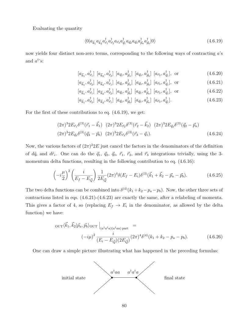
Evaluating the quantity

〈0|a~k1a~k2a†~r1a†~r2a~r3a

†~q1a~q2a~q3a

†~paa†~pb|0〉 (4.6.19)

now yields four distinct non-zero terms, corresponding to the following ways of contracting a’s

and a†’s:

[a~k1 , a†~r1] [a~k2 , a

†~r2] [a~q2 , a

†~pa] [a~q3 , a

†~pb] [a~r3 , a

†~q1], or (4.6.20)

[a~k1 , a†~r2] [a~k2 , a

†~r1] [a~q2 , a

†~pa] [a~q3 , a

†~pb] [a~r3 , a

†~q1], or (4.6.21)

[a~k1 , a†~r1] [a~k2 , a

†~r2] [a~q2 , a

†~pb] [a~q3 , a

†~pa] [a~r3 , a

†~q1], or (4.6.22)

[a~k1 , a†~r2] [a~k2 , a

†~r1] [a~q2 , a

†~pb] [a~q3 , a

†~pa] [a~r3 , a

†~q1]. (4.6.23)

For the first of these contributions to eq. (4.6.19), we get:

(2π)32E~r1δ(3)(~r1 − ~k1) (2π)32E~r2δ

(3)(~r2 − ~k2) (2π)32E~q2δ(3)(~q2 − ~pa)

(2π)32E~q3δ(3)(~q3 − ~pb) (2π)32E~r3δ

(3)(~r3 − ~q1). (4.6.24)

Now, the various factors of (2π)22E just cancel the factors in the denominators of the definition

of dqi and dri. One can do the ~q1, ~q2, ~q3, ~r1, ~r2, and ~r3 integrations trivially, using the 3-

momentum delta functions, resulting in the following contribution to eq. (4.6.16):

(−iµ

2

)2(

i

Ef − E ~Q

)1

2E ~Q

(2π)4δ(Ef − Ei)δ(3)(~k1 + ~k2 − ~pa − ~pb). (4.6.25)

The two delta functions can be combined into δ(4)(k1+k2−pa−pb). Now, the other three sets ofcontractions listed in eqs. (4.6.21)-(4.6.23) are exactly the same, after a relabeling of momenta.

This gives a factor of 4, so (replacing Ef → Ei in the denominator, as allowed by the delta

function) we have:

OUT〈~k1, ~k2|~pa, ~pb〉OUT

∣∣∣(a†a†a)(a†aa) part

=

(−iµ)2 i

(Ei − E ~Q)(2E ~Q)(2π)4δ(4)(k1 + k2 − pa − pb). (4.6.26)

One can draw a simple picture illustrating what has happened in the preceding formulas:

initial state final statea†a†aa†aa

80

The initial state contains two particles, denoted by the lines on the left. Acting with the first

factor of Hint (on the right in the formula, and represented by the vertex on the left in the

figure) destroys the two particles and creates a virtual particle in their place. The second factor

of Hint destroys the virtual particle and creates the two final state particles, represented by

the lines on the right. The three-momentum carried by the intermediate virtual particle is

~Q = ~pa + ~pb = ~k1 + ~k2, so momentum is conserved at the two vertices.

However, there are other contributions that must be included. Another one occurs if the Hint

on the right in eq. (4.6.15) contains a†a†a† operators, and the other Hint contains aaa operators.

The corresponding picture is this:

initial state final state

aaa

a†a†a†

Here the Hint carrying a†a†a† (the rightmost one in the formula) is represented by the upper

left vertex in the figure, and the one carrying aaa is represented by the lower right vertex. The

explicit formula corresponding to this picture is:

OUT〈~k1, ~k2|~pa, ~pb〉OUT

∣∣∣(aaa)(a†a†a†) part

=[−iµ

6(2π)3

]22πδ(Ef − Ei)

∫dr1

∫dr2

∫dr3

∫dq1

∫dq2

∫dq3

δ(3)(~r1 + ~r2 + ~r3) δ(3)(~q1 + ~q2 + ~q3)

〈0|a~k1a~k2a~r1a~r2a~r3(

i

Ef − EX

)a†~q1a

†~q2a†~q3a

†~paa†~pb |0〉. (4.6.27)

As before, we can calculate this by commuting a’s to the right and a†’s to the left. In the end,

non-zero contributions arise only when each a is contracted with some a†. In doing so, we should

ignore any terms that arise whenever a final state state a~k is contracted with an initial state a†~p.

That would correspond to a situation with no scattering, since the initial state particle and the

final state particle would be exactly the same.

The result contains 36 distinct contributions, corresponding to the 6 ways of contracting

a~k1 and a~k2 with any two of a†~q1 , a†~q2, and a†~q3 , times the 6 ways of contracting a†~pa and a†~pb with

any two of a~r1 , a~r2 , a~r3 . However, all 36 of these contributions are identical under relabeling

of momentum, so we can just calculate one of them and multiply the answer by 36. This will

neatly convert the factor of (−iµ/6)2 to (−iµ)2. We also note that EX must be replaced by the

81

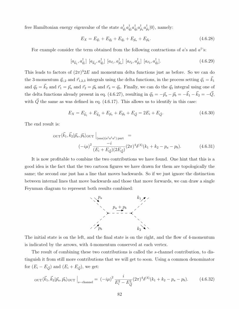
free Hamiltonian energy eigenvalue of the state a†~q1a†~q2a†~q3a

†~paa†~pb |0〉, namely:

EX = E~q1 + E~q2 + E~q3 + E~pa + E~pb . (4.6.28)

For example consider the term obtained from the following contractions of a’s and a†’s:

[a~k1 , a†~q1] [a~k2 , a

†~q2] [a~r1 , a

†~pa] [a~r2 , a

†~pb] [a~r3 , a

†~q3]. (4.6.29)

This leads to factors of (2π)32E and momentum delta functions just as before. So we can do

the 3-momentum ~q1,2 and ~r1,2,3 integrals using the delta functions, in the process setting ~q1 = ~k1

and ~q2 = ~k2 and ~r1 = ~pa and ~r2 = ~pb and ~r3 = ~q3. Finally, we can do the ~q3 integral using one of

the delta functions already present in eq. (4.6.27), resulting in ~q3 = −~pa− ~pb = −~k1−~k2 = − ~Q,with ~Q the same as was defined in eq. (4.6.17). This allows us to identify in this case:

EX = E~k1+ E~k2

+ E~pa + E~pb + E ~Q = 2Ei + E ~Q. (4.6.30)

The end result is:

OUT〈~k1, ~k2|~pa, ~pb〉OUT

∣∣∣(aaa)(a†a†a†) part

=

(−iµ)2 −i(Ei + E ~Q)(2E ~Q)

(2π)4δ(4)(k1 + k2 − pa − pb). (4.6.31)

It is now profitable to combine the two contributions we have found. One hint that this is a

good idea is the fact that the two cartoon figures we have drawn for them are topologically the

same; the second one just has a line that moves backwards. So if we just ignore the distinction

between internal lines that move backwards and those that move forwards, we can draw a single

Feynman diagram to represent both results combined:

pa k1

pb k2

pa + pb

The initial state is on the left, and the final state is on the right, and the flow of 4-momentum

is indicated by the arrows, with 4-momentum conserved at each vertex.

The result of combining these two contributions is called the s-channel contribution, to dis-

tinguish it from still more contributions that we will get to soon. Using a common denominator

for (Ei − E ~Q) and (Ei + E ~Q), we get:

OUT〈~k1, ~k2|~pa, ~pb〉OUT

∣∣∣s−channel

= (−iµ)2 i

E2i − E2

~Q

(2π)4δ(4)(k1 + k2 − pa − pb). (4.6.32)

82

If we now consider the four-vector

pµa + pµb = (√|~pa|2 +m2 +

√|~pb|2 +m2 , ~pa + ~pb) = (Ei, ~Q), (4.6.33)

then we recognize that

(pa + pb)2 = E2

i − | ~Q|2 = E2i − E2

~Q+m2. (4.6.34)

[Note that pµa + pµb is not equal to (E ~Q,~Q).] So we can rewrite the term

i

E2i − E2

~Q

=i

(pa + pb)2 −m2, (4.6.35)

The final result is that the s-channel contribution to the matrix element is:

OUT〈~k1, ~k2|~pa, ~pb〉OUT

∣∣∣s−channel

= (−iµ)2 i

(pa + pb)2 −m2(2π)4δ(4)(k1 + k2 − pa − pb). (4.6.36)

Note that one could just as well have put (k1 + k2)2 in place of (pa + pb)

2 in this expression,

because of the delta function.

Now one can go through the same whole process with contributions that come from the

rightmost Hint (acting first on the initial state) consisting of a†a†a terms, and the leftmost Hint

containing a†aa terms. One can draw Feynman diagrams that represent these terms, which look

like:

k2

k1

pb

pa

pa − k1

k2

k1

pb

pa

pa − k2

These are referred to as the t-channel and u-channel contributions respectively. Here we have

combined all topologically-identical diagrams. This is a standard procedure that is always

followed; the diagrams we have drawn with dashed lines for the scalar field are the Feynman

diagrams for the process. [The solid-line diagrams appearing between eqs. (4.6.26) and (4.6.27)

above are sometimes known as “old-fashioned Feynman diagrams”, but it is very rare to see

them in the modern literature.]

After much juggling of factors of (2π)3 and doing 3-momentum integrals using delta functions,

but using no new concepts, the contributions of the t-channel and u-channel Feynman diagrams

can be found to be simply:

OUT〈~k1, ~k2|~pa, ~pb〉OUT

∣∣∣t−channel

= (−iµ)2 i

(pa − k1)2 −m2(2π)4δ(4)(k1 + k2 − pa − pb), (4.6.37)

83

and

OUT〈~k1, ~k2|~pa, ~pb〉OUT

∣∣∣u−channel

= (−iµ)2 i

(pa − k2)2 −m2(2π)4δ(4)(k1 + k2 − pa − pb). (4.6.38)

The reduced matrix element can now be obtained by just stripping off the factors of (2π)4δ(4)(k1+

k2 − pa − pb), as demanded by the definition eq. (4.5.11). So the total reduced matrix element,

suitable for plugging into the formula for the cross-section, is:

Mφφ→φφ = Ms +Mt +Mu (4.6.39)

where:

Ms = (−iµ)2 i

(pa + pb)2 −m2, (4.6.40)

Mt = (−iµ)2 i

(pa − k1)2 −m2, (4.6.41)

Mu = (−iµ)2 i

(pa − k2)2 −m2. (4.6.42)

The reason for the terminology s, t, and u is because of the standard kinematic variables for

2→2 scattering known as Mandelstam variables:

s = (pa + pb)2 = (k1 + k2)

2, (4.6.43)

t = (pa − k1)2 = (k2 − pb)2, (4.6.44)

u = (pa − k2)2 = (k1 − pb)2. (4.6.45)

The s-, t-, and u-channel diagrams are simple functions of the corresponding Mandelstam vari-

ables:

Ms = (−iµ)2 i

s−m2, (4.6.46)

Mt = (−iµ)2 i

t−m2, (4.6.47)

Mu = (−iµ)2 i

u−m2. (4.6.48)

Typically, if one instead scatters fermions or vector particles or some combination of them, the

s- t- and u- channel diagrams will have a similar form, with m always the mass of the particle

on the internal line, but with more junk in the numerators coming from the appropriate reduced

matrix elements.

4.7 Feynman rules

It is now possible to abstract what we have found, to obtain the general Feynman rules for

calculating reduced matrix elements in a scalar field theory. Evidently, the reduced matrix

84

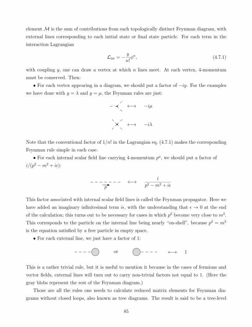
elementM is the sum of contributions from each topologically distinct Feynman diagram, with

external lines corresponding to each initial state or final state particle. For each term in the

interaction Lagrangian

Lint = −y

n!φn, (4.7.1)

with coupling y, one can draw a vertex at which n lines meet. At each vertex, 4-momentum

must be conserved. Then:

• For each vertex appearing in a diagram, we should put a factor of −iy. For the examples

we have done with y = λ and y = µ, the Feynman rules are just:

←→ −iµ

←→ −iλ

Note that the conventional factor of 1/n! in the Lagrangian eq. (4.7.1) makes the corresponding

Feynman rule simple in each case.

• For each internal scalar field line carrying 4-momentum pµ, we should put a factor of

i/(p2 −m2 + iǫ):

p←→ i

p2 −m2 + iǫ

This factor associated with internal scalar field lines is called the Feynman propagator. Here we

have added an imaginary infinitesimal term iǫ, with the understanding that ǫ → 0 at the end

of the calculation; this turns out to be necessary for cases in which p2 become very close to m2.

This corresponds to the particle on the internal line being nearly “on-shell”, because p2 = m2

is the equation satisfied by a free particle in empty space.

• For each external line, we just have a factor of 1:

or ←→ 1

This is a rather trivial rule, but it is useful to mention it because in the cases of fermions and

vector fields, external lines will turn out to carry non-trivial factors not equal to 1. (Here the

gray blobs represent the rest of the Feynman diagram.)

Those are all the rules one needs to calculate reduced matrix elements for Feynman dia-

grams without closed loops, also known as tree diagrams. The result is said to be a tree-level

85

calculation. There are additional rules that apply to diagrams with closed loops (loop diagrams)

which have not arisen explicitly in the preceding discussion, but could be inferred from more

complicated calculations. For them, the additional rules are:

• For each closed loop in a Feynman diagram, there is an undetermined 4-momentum ℓµ.

These loop momenta should be integrated over according to:

∫ d4ℓ

(2π)4. (4.7.2)

Loop diagrams quite often diverge because of the integration over all ℓµ, because of the con-

tribution from very large |ℓ2|. This can be fixed by introducing a cutoff |ℓ2|max in the integral,

or by other more rigorous methods, which can make the integrals finite. The techniques of

getting physically meaningful answers out of this are known as regularization (making the inte-

grals finite) and renormalization (redefining coupling constants and masses so that the physical

observables do not depend explicitly on the unknown cutoff).

• If a Feynman diagram with one or more closed loops can be transformed into an exact copy

of itself by interchanging any number of internal lines through a smooth deformation, without

moving the external lines, then there is an additional factor of 1/N , where N is the number

of distinct permutations of that type. (This is known as the “symmetry factor” for the loop

diagram.)

Some examples might be useful. In the φ3 theory, there are quite a few Feynman diagrams

that will describe the scattering of 2 particles to 3 particles. One of them is shown below:

pa

k1

k1 + k2

pb

k2

k3

pa + pb

For this diagram, according to the rules, the contribution to the reduced matrix element is just

M = (−iµ)3[

i

(pa + pb)2 −m2

] [i

(k1 + k2)2 −m2

]. (4.7.3)

Imagine having to calculate this starting from scratch with creation and annihilation operators,

and tremble with fear! Feynman rules are good.

An example of a Feynman diagram with a closed loop in the φ3 theory is:

86

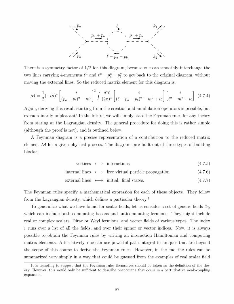
pa k1

pb k2

pa + pb pa + pb

ℓ

ℓ− pa − pb

There is a symmetry factor of 1/2 for this diagram, because one can smoothly interchange the

two lines carrying 4-momenta ℓµ and ℓµ − pµa − pµb to get back to the original diagram, without

moving the external lines. So the reduced matrix element for this diagram is:

M =1

2(−iµ)4

[i

(pa + pb)2 −m2

]2 ∫ d4ℓ

(2π)4

[i

(ℓ− pa − pb)2 −m2 + iǫ

] [i

ℓ2 −m2 + iǫ

]. (4.7.4)

Again, deriving this result starting from the creation and annihilation operators is possible, but

extraordinarily unpleasant! In the future, we will simply state the Feynman rules for any theory

from staring at the Lagrangian density. The general procedure for doing this is rather simple

(although the proof is not), and is outlined below.

A Feynman diagram is a precise representation of a contribution to the reduced matrix

elementM for a given physical process. The diagrams are built out of three types of building

blocks:

vertices ←→ interactions (4.7.5)

internal lines ←→ free virtual particle propagation (4.7.6)

external lines ←→ initial, final states. (4.7.7)

The Feynman rules specify a mathematical expression for each of these objects. They follow

from the Lagrangian density, which defines a particular theory.†

To generalize what we have found for scalar fields, let us consider a set of generic fields Φi,

which can include both commuting bosons and anticommuting fermions. They might include

real or complex scalars, Dirac or Weyl fermions, and vector fields of various types. The index

i runs over a list of all the fields, and over their spinor or vector indices. Now, it is always

possible to obtain the Feynman rules by writing an interaction Hamiltonian and computing

matrix elements. Alternatively, one can use powerful path integral techniques that are beyond

the scope of this course to derive the Feynman rules. However, in the end the rules can be

summarized very simply in a way that could be guessed from the examples of real scalar field

†It is tempting to suggest that the Feynman rules themselves should be taken as the definition of the the-ory. However, this would only be sufficient to describe phenomena that occur in a perturbative weak-couplingexpansion.

87

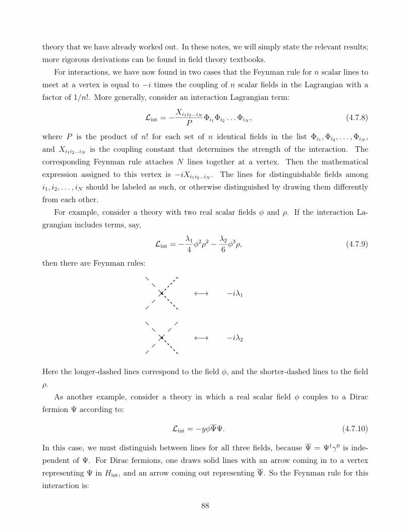
theory that we have already worked out. In these notes, we will simply state the relevant results;

more rigorous derivations can be found in field theory textbooks.

For interactions, we have now found in two cases that the Feynman rule for n scalar lines to

meet at a vertex is equal to −i times the coupling of n scalar fields in the Lagrangian with a

factor of 1/n!. More generally, consider an interaction Lagrangian term:

Lint = −Xi1i2...iN

PΦi1Φi2 . . .ΦiN , (4.7.8)

where P is the product of n! for each set of n identical fields in the list Φi1 ,Φi2 , . . . ,ΦiN ,

and Xi1i2...iN is the coupling constant that determines the strength of the interaction. The

corresponding Feynman rule attaches N lines together at a vertex. Then the mathematical

expression assigned to this vertex is −iXi1i2...iN . The lines for distinguishable fields among

i1, i2, . . . , iN should be labeled as such, or otherwise distinguished by drawing them differently

from each other.

For example, consider a theory with two real scalar fields φ and ρ. If the interaction La-

grangian includes terms, say,

Lint = −λ14φ2ρ2 − λ2

6φ3ρ, (4.7.9)

then there are Feynman rules:

←→ −iλ1

←→ −iλ2

Here the longer-dashed lines correspond to the field φ, and the shorter-dashed lines to the field

ρ.

As another example, consider a theory in which a real scalar field φ couples to a Dirac

fermion Ψ according to:

Lint = −yφΨΨ. (4.7.10)

In this case, we must distinguish between lines for all three fields, because Ψ = Ψ†γ0 is inde-

pendent of Ψ. For Dirac fermions, one draws solid lines with an arrow coming in to a vertex

representing Ψ in Hint, and an arrow coming out representing Ψ. So the Feynman rule for this

interaction is:

88

←→ −iyδab

b

a

Note that this Feynman rule is proportional to a 4 × 4 identity matrix in Dirac spinor space.

This is because the interaction Lagrangian can be written −yδabφΨaΨb, where a is the Dirac

spinor index for Ψ and b for Ψ. Often, one just suppresses the spinor indices, and writes simply

−iy for the Feynman rule, with the identity matrix implicit.

The interaction Lagrangian eq. (4.7.10) is called a Yukawa coupling. This theory has a

real-world physical application: it is precisely the type of interaction that applies between the

Standard Model Higgs boson φ = h and each Dirac fermion Ψ, with the coupling y proportional

to the mass of that fermion. We will return to this interaction when we discuss the decays of

the Higgs boson into fermion-antifermion pairs.

Let us turn next to the topic of internal lines in Feynman diagrams. These are determined

by the free (quadratic) part of the Lagrangian density. Recall that for a scalar field, we can

write the free Lagrangian after integrating by parts as:

L0 =1

2φ(−∂µ∂µ −m2)φ. (4.7.11)

This corresponded to a Feynman propagator rule for internal scalar lines i/(p2−m2+ iǫ). So, up

to the iǫ factor, the propagator is just proportional to i divided by the inverse of the coefficient

of the quadratic piece of the Lagrangian density, with the replacement

∂µ −→ −ipµ. (4.7.12)

The free Lagrangian density for generic fields Φi can always be put into either the form

L0 =1

2

∑

i,j

ΦiPijΦj , (4.7.13)

for real fields, or the form

L0 =∑

i,j

(Φ†)iPijΦj , (4.7.14)

for complex fields (including, for example, Dirac spinors). To accomplish this, one may need to

integrate the action by parts, throwing away a total derivative in L0 which will not contribute

to S =∫d4x L. Here Pij is a matrix that involves spacetime derivatives and masses. Then it

turns out that the Feynman propagator can be found by making the replacement eq. (4.7.12)

and taking i times the inverse of the matrix Pij:

i(P−1)ij. (4.7.15)

89

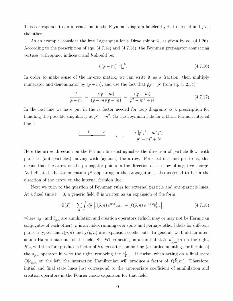
This corresponds to an internal line in the Feynman diagram labeled by i at one end and j at

the other.

As an example, consider the free Lagrangian for a Dirac spinor Ψ, as given by eq. (4.1.26).

According to the prescription of eqs. (4.7.14) and (4.7.15), the Feynman propagator connecting

vertices with spinor indices a and b should be:

i[(/p−m)−1]ab. (4.7.16)

In order to make sense of the inverse matrix, we can write it as a fraction, then multiply

numerator and denominator by (/p+m), and use the fact that /p/p = p2 from eq. (3.2.54):

i

/p−m=

i(/p+m)

(/p−m)(/p+m)=

i(/p+m)

p2 −m2 + iǫ. (4.7.17)

In the last line we have put in the iǫ factor needed for loop diagrams as a prescription for

handling the possible singularity at p2 = m2. So the Feynman rule for a Dirac fermion internal

line is:

←→ i([/p]ab +mδa

b)

p2 −m2 + iǫ

b ap→

Here the arrow direction on the fermion line distinguishes the direction of particle flow, with

particles (anti-particles) moving with (against) the arrow. For electrons and positrons, this

means that the arrow on the propagator points in the direction of the flow of negative charge.

As indicated, the 4-momentum pµ appearing in the propagator is also assigned to be in the

direction of the arrow on the internal fermion line.

Next we turn to the question of Feynman rules for external particle and anti-particle lines.

At a fixed time t = 0, a generic field Φ is written as an expansion of the form:

Φ(~x) =∑

n

∫dp

[i(~p, n) ei~p·~xa~p,n + f(~p, n) e−i~p·~xb†~p,n

], (4.7.18)

where a~p,n and b†~p,n are annihilation and creation operators (which may or may not be Hermitian

conjugates of each other); n is an index running over spins and perhaps other labels for different

particle types; and i(~p, n) and f(~p, n) are expansion coefficients. In general, we build an inter-

action Hamiltonian out of the fields Φ. When acting on an initial state a†~k,m|0〉 on the right,

Hint will therefore produce a factor of i(~k,m) after commuting (or anticommuting, for fermions)

the a~p,n operator in Φ to the right, removing the a†~k,m. Likewise, when acting on a final state

〈0|b~k,m on the left, the interaction Hamiltonian will produce a factor of f(~k,m). Therefore,

initial and final state lines just correspond to the appropriate coefficient of annihilation and

creation operators in the Fourier mode expansion for that field.

90

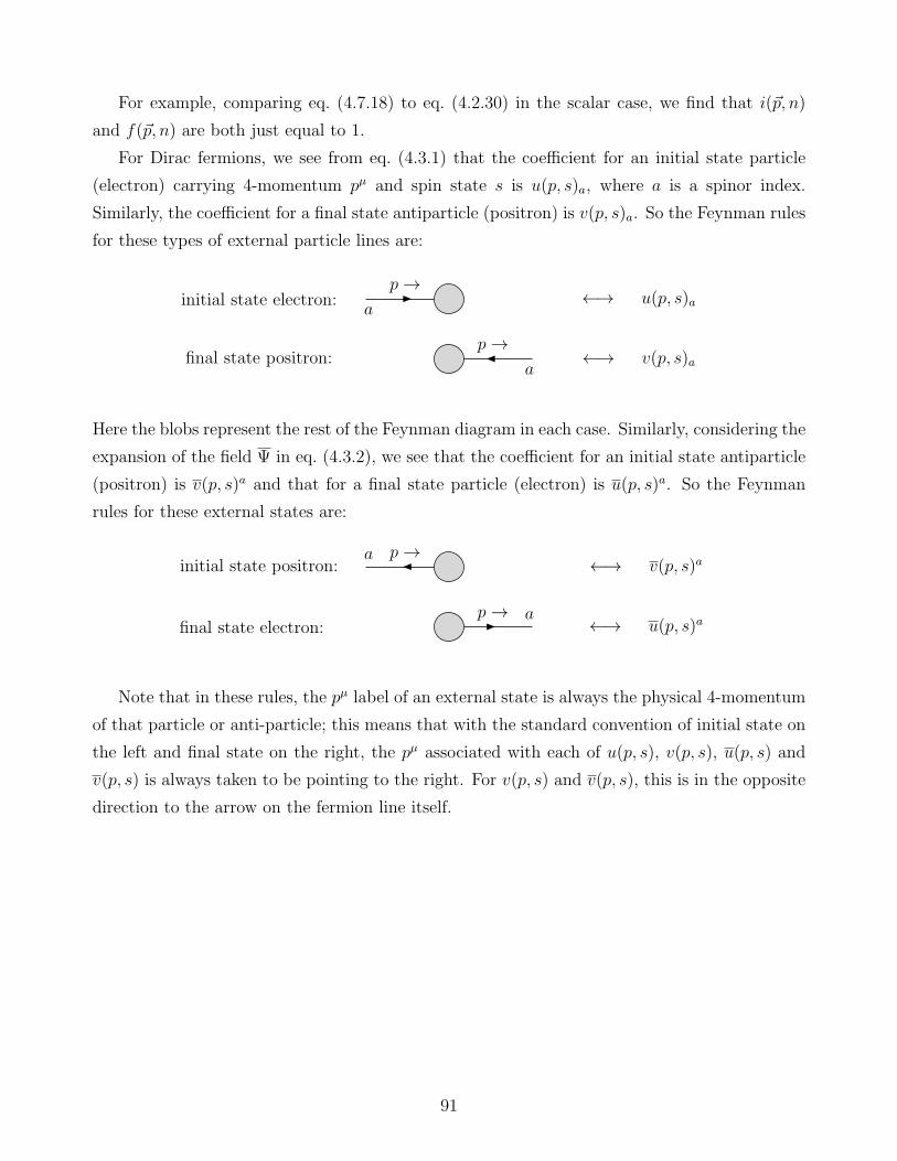
For example, comparing eq. (4.7.18) to eq. (4.2.30) in the scalar case, we find that i(~p, n)

and f(~p, n) are both just equal to 1.

For Dirac fermions, we see from eq. (4.3.1) that the coefficient for an initial state particle

(electron) carrying 4-momentum pµ and spin state s is u(p, s)a, where a is a spinor index.

Similarly, the coefficient for a final state antiparticle (positron) is v(p, s)a. So the Feynman rules

for these types of external particle lines are:

a

p→initial state electron: ←→ u(p, s)a

a

p→final state positron: ←→ v(p, s)a

Here the blobs represent the rest of the Feynman diagram in each case. Similarly, considering the

expansion of the field Ψ in eq. (4.3.2), we see that the coefficient for an initial state antiparticle

(positron) is v(p, s)a and that for a final state particle (electron) is u(p, s)a. So the Feynman

rules for these external states are:

a p→←→ v(p, s)ainitial state positron:

ap→←→ u(p, s)afinal state electron:

Note that in these rules, the pµ label of an external state is always the physical 4-momentum

of that particle or anti-particle; this means that with the standard convention of initial state on

the left and final state on the right, the pµ associated with each of u(p, s), v(p, s), u(p, s) and

v(p, s) is always taken to be pointing to the right. For v(p, s) and v(p, s), this is in the opposite

direction to the arrow on the fermion line itself.

91

5 Quantum Electro-Dynamics (QED)

5.1 QED Lagrangian and Feynman rules

Let us now see how all of these general rules apply in the case of Quantum Electrodynamics. This

is the quantum field theory governing photons (quantized electromagnetic waves) and charged

fermions and antifermions. The fermions in the theory are represented by Dirac spinor fields

Ψ carrying electric charge Qe, where e is the magnitude of the charge of the electron. Thus

Q = −1 for electrons and positrons, +2/3 for up, charm and top quarks and their anti-quarks,

and −1/3 for down, strange and bottom quarks and their antiquarks. (Recall that a single Dirac

field, assigned a single value of Q, is used to describe both particles and their anti-particles.)

The free Lagrangian for the theory is:

L0 = −1

4F µνFµν +Ψ(iγµ∂µ −m)Ψ. (5.1.1)

Now, earlier we found that the electromagnetic field Aµ couples to the 4-current density

Jµ = (ρ, ~J ) by a term in the Lagrangian −eJµAµ [see eq. (4.1.39)]. Since Jµ must be a

four-vector built out of the charged fermion fields Ψ and Ψ, we can guess that

Jµ = QΨγµΨ. (5.1.2)

The interaction Lagrangian density for a fermion with charge Qe and electromagnetic fields is

therefore

Lint = −eQΨγµΨAµ. (5.1.3)

The value of e is determined by experiment. However, it is a running coupling constant, which

means that effectively its value has a logarithmic dependence on the characteristic energy of the

process. For very low energy experiments, the numerical value is e ≈ 0.30282, corresponding to

the experimental result for the fine structure constant:

α ≡ e2

4π≈ 1/137.036. (5.1.4)

For experiments done at energies near 100 GeV, the appropriate value is a little larger, more

like e ≈ 0.313.

Let us take a small detour to check that eq. (5.1.2) really has the correct form and normal-

ization to be the electromagnetic current density. Consider the total charge operator:

Q =∫d3~x ρ(~x) =

∫d3~x J0(~x) = Q

∫d3~xΨγ0Ψ = Q

∫d3~xΨ†Ψ. (5.1.5)

92

Plugging in eqs. (4.3.1) and (4.3.2), and doing the ~x integration, and one of the momentum

integrations using the resulting delta function, one finds

Q = Q2∑

s=1

2∑

r=1

∫dp

1

2E~p

[u†(p, s)b†~p,s + v†(p, s)d~p,s] [u(p, r)b~p,r + v(p, r)d†~p,r]. (5.1.6)

This can be simplified using some spinor identities:

u†(p, s)u(p, r) = v†(p, s)v(p, r) = 2E~p δsr; (5.1.7)

u†(p, s)v(p, r) = v†(p, s)u(p, r) = 0. (5.1.8)

Taking into account that the operators d, d† satisfy the anticommutation relation eqs. (4.3.20),

the result is

Q = Q2∑

s=1

∫dp

[b†~p,sb~p,s − d†~p,sd~p,s

]. (5.1.9)

Here we have dropped an infinite contribution, much like we had to do in getting to eqs. (4.2.42)

and eqs. (4.3.21). This represents a uniform and constant (and therefore unobservable) infinite

charge density throughout all space. The result is that the total charge eigenvalue of the vacuum

vanishes:

Q|0〉 = 0. (5.1.10)

One can now check that

[Q, b†~k,r] = Qb†~k,r, (5.1.11)

[Q, d†~k,r] = −Qd†~k,r. (5.1.12)

Therefore,

Q b†~k,r|0〉 = Q b†~k,r|0〉 (5.1.13)

for single-particle states, and

Q d†~k,r|0〉 = −Q d†~k,r|0〉 (5.1.14)

for single anti-particle states. More generally, the eigenvalue of Q acting on a state with N

particles and N antiparticles is (N−N)Q. From eq. (5.1.5), this verifies that the charge density

ρ is indeed the time-like component of the four-vector QΨγµΨ, which must therefore be equal

to Jµ.

93

The full QED Lagrangian is invariant under gauge transformations:

Aµ(x) → Aµ(x)−1

e∂µθ(x), (5.1.15)

Ψ(x) → eiQθ Ψ(x), (5.1.16)

Ψ(x) → e−iQθ Ψ(x), (5.1.17)

where θ(x) is an arbitrary function of spacetime [equal to −eλ(x) in eq. (2.4.16)]. A nice way

to see this invariance is to define the covariant derivative:

DµΨ ≡ (∂µ + iQeAµ)Ψ. (5.1.18)

Here the term “covariant” refers to the gauge transformation symmetry, not the Lorentz trans-

formation symmetry as it did when we introduced covariant four-vectors. Note that the covariant

derivative actually depends on the charge of the field it acts on. Now one can write the full

Lagrangian density as

L = L0 + Lint = −1

4F µνFµν + iΨγµDµΨ−mΨΨ. (5.1.19)

The ordinary derivative of the spinor transforms under the gauge transformation with an “extra”

term:

∂µΨ → ∂µ(eiQθΨ) = eiQθ∂µΨ+ iQΨ∂µθ. (5.1.20)

The point of the covariant derivative of Ψ is that it transforms under the gauge transformation

the same way Ψ does, by acquiring a phase:

DµΨ → eiQθDµΨ. (5.1.21)

Here the contribution from the transformation of Aµ in Dµ cancels the extra term in eq. (5.1.20).

Using eqs. (5.1.15)-(5.1.17) and (5.1.21), it is easy to see that L is invariant under the gauge

transformation, since the multiplicative phase factors just cancel.

Returning to the interaction term eq. (5.1.3), we can now identify the Feynman rule for QED

interactions, by following the general prescription outlined with eq. (4.7.8):

←→ −iQeγµ

b

a

µ

This one interaction vertex governs all physical processes in QED.

94

To find the Feynman rules for initial and final state photons, consider the Fourier expansion

of the vector field at a fixed time:

Aµ =3∑

λ=0

∫dp

[ǫµ(p, λ)e

i~p·~xa~p,λ + ǫ∗µ(p, λ)e−i~p·~xa†~p,λ

]. (5.1.22)

Here ǫµ(p, λ) is a basis of four polarization four-vectors labeled by λ = 0, 1, 2, 3. They satisfy

the orthonormality condition:

ǫµ(p, λ)ǫ∗µ(p, λ′) =

−1 for λ = λ′ = 1, 2, or 3+1 for λ = λ′ = 00 for λ 6= λ′

(5.1.23)

The operators a†~p,λ and a~p,λ act on the vacuum state by creating and destroying photons with

momentum ~p and polarization vector ǫµ(p, λ).

However, not all of the four degrees of freedom labeled by λ can be physical. From classical

electromagnetism, we know that electromagnetic waves are transversely polarized. This means

that the electric and magnetic fields are perpendicular to the 3-momentum direction of propa-

gation. In terms of the potentials, it means that one can always choose a gauge in which A0 = 0

and the Lorenz gauge condition ∂µAµ = 0 is satisfied. Therefore, physical electromagnetic wave

quanta corresponding to the classical solutions to Maxwell’s equations Aµ = ǫµe−ip·x with p2 = 0

can be taken to obey:

ǫµ = (0,~ǫ), (5.1.24)

pµǫµ = 0 (5.1.25)

(or, equivalent to the last condition, ~ǫ · ~p = 0). After imposing these two conditions, only two

of the four λ’s will survive as valid initial or final states for any given pµ.

For example, suppose that a state contains a photon with 3-momentum ~p = pz, so pµ =

(p, 0, 0, p). Then we can choose a basis of transverse linearly-polarized vectors with λ = 1, 2:

ǫµ(p, 1) = (0, 1, 0, 0) x-polarized, (5.1.26)

ǫµ(p, 2) = (0, 0, 1, 0) y-polarized. (5.1.27)

However, in high-energy physics it is often more useful to instead use a basis of left- and right-

handed circular polarizations that carry definite helicities λ = R,L:

ǫµ(p,R) =1√2(0, 1, i, 0) right-handed, (5.1.28)

ǫµ(p, L) =1√2(0, 1,−i, 0) left-handed. (5.1.29)

95

In general, incoming photon lines have a Feynman rule ǫµ(p, λ) and outgoing photon lines have

a Feynman rule ǫ∗µ(p, λ), where λ = 1, 2 in some convenient basis of choice. Often, we will sum

or average over the polarization labels λ, so the ǫµ(p, λ) will not need to be listed explicitly for

a given momentum.

Let us next construct the Feynman propagator for photon lines. The free Lagrangian density

given in eq. (4.1.34) can be rewritten as:

L0 =1

2Aµ (gµν∂ρ∂

ρ − ∂µ∂ν)Aν , (5.1.30)

where we have dropped a total derivative. (The action, obtained by integrating L0, does not

depend on total derivative terms.) Therefore, following the prescription of eq. (4.7.15), it appears

that we ought to find the propagator by finding the inverse of the 4× 4 matrix

Pµν = −p2gµν + pµpν . (5.1.31)

Unfortunately, however, this matrix is not invertible. The reason for this can be traced to the

gauge invariance of the theory; not all of the physical states we are attempting to propagate are

really physical.

This problem can be avoided using a trick, due to Fermi, called “gauge fixing”. As long as

we agree to stick to the Lorenz gauge, ∂µAµ = 0, we can add a term to the Lagrangian density

proportional to (∂µAµ)2:

L(ξ)0 = L0 −

1

2ξ(∂µA

µ)2. (5.1.32)

In Lorenz gauge, not only does the extra term vanish, but also its contribution to the equations

of motion vanishes. Here ξ is an arbitrary new gauge-fixing parameter; it can be picked at will.

Intermediate steps in a calculation may depend on it, but physical results should not depend

on the choice of ξ. The new term in the modified free Lagrangian L(ξ)0 is called the gauge-fixing

term. Now the matrix to be inverted is:

Pµν = −p2gµν +(1− 1

ξ

)pµpν . (5.1.33)

To find the inverse, one notices that as a tensor, (P−1)νρ can only be a linear combination of

terms proportional to gνρ and to pνpρ. So, writing the most general possible form for the answer:

(P−1)νρ = C1 gνρ + C2 p

νpρ (5.1.34)

and requiring that

Pµν(P−1)νρ = δρµ, (5.1.35)

96

one finds the solution

C1 = − 1

p2; C2 =

1− ξ(p2)2

. (5.1.36)

It follows that the desired Feynman propagator for a photon with momentum pµ is:

i

p2 + iǫ

[−gµν + (1− ξ)pµpν

p2

]. (5.1.37)

(Here we have put in the iǫ factor in the denominator as usual.) In a Feynman diagram, this

propagator corresponds to an internal wavy line, labeled by µ and ν at opposite ends, and

carrying 4-momentum p. The gauge-fixing parameter ξ can be chosen at the convenience or

whim of the person computing the Feynman diagram. The most popular choice for simple

calculations is ξ = 1, called Feynman gauge. Then the Feynman propagator for photons is

simply:

−igµνp2 + iǫ

(Feynman gauge). (5.1.38)

Another common choice is ξ = 0, known as Landau gauge, for which the Feynman propagator

is:

−ip2 + iǫ

[gµν −

pµpνp2

](Landau gauge). (5.1.39)

[Comparing to eq. (5.1.32), we see that this is really obtained as a formal limit ξ → 0.] The

Landau gauge photon propagator has the nice property that it vanishes when contracted with

either pµ or pν , which can make some calculations simpler (especially certain loop diagram

calculations). Sometimes it is useful to just leave ξ unspecified. Even though this means having

to calculate more terms, the payoff is that in the end one can see if the final answer for the

reduced matrix element is independent of ξ, providing a consistency check.

We have now encountered most of the Feynman rules for QED. There are some additional

rules having to do with minus signs because of Fermi-Dirac statistics; these can be understood

by carefully considering the effects of anticommutation relations for fermionic operators. In

practice, one usually does not write out the spinor indices explicitly. All of the rules are sum-

marized in the following two pages in a cookbook form. Of course, the best way to understand

how the rules work is to do some examples. That will be the subject of the next few subsections.

97

Feynman rules for QED

To find the contributions to the reduced matrix element M for a physical process involving

charged Dirac fermions and photons:

1. Draw all topologically distinct Feynman diagrams, with wavy lines representing photons, and

solid lines with arrows representing fermions, using the rules below for external lines, internal

lines, and interaction vertices. The arrow direction is preserved when following each fermion

line. Enforce four-momentum conservation at each vertex.

2. For external lines, write (with 4-momentum pµ always to the right, and spin polarization s

or λ as appropriate):

initial-state fermion: ←→ u(p, s)

←→ v(p, s)initial-state antifermion:

←→ u(p, s)final-state fermion:

final-state antifermion: ←→ v(p, s)

µ←→ ǫµ(p, λ)initial-state photon:

µfinal-state photon: ←→ ǫ∗µ(p, λ)

3. For internal fermion lines, write Feynman propagators:

←→ i(/p+m)

p2 −m2 + iǫ

with 4-momentum pµ along the arrow direction, and m the mass of the fermion. For internal

photon lines, write:

←→ i

p2 + iǫ

[−gµν + (1− ξ)pµpν

p2

]µ ν

with 4-momentum pµ along either direction in the wavy line. (Use ξ = 1 for Feynman gauge

and ξ = 0 for Landau gauge.)

4. For the interaction vertex of a fermion f of charge Qf , write:

98

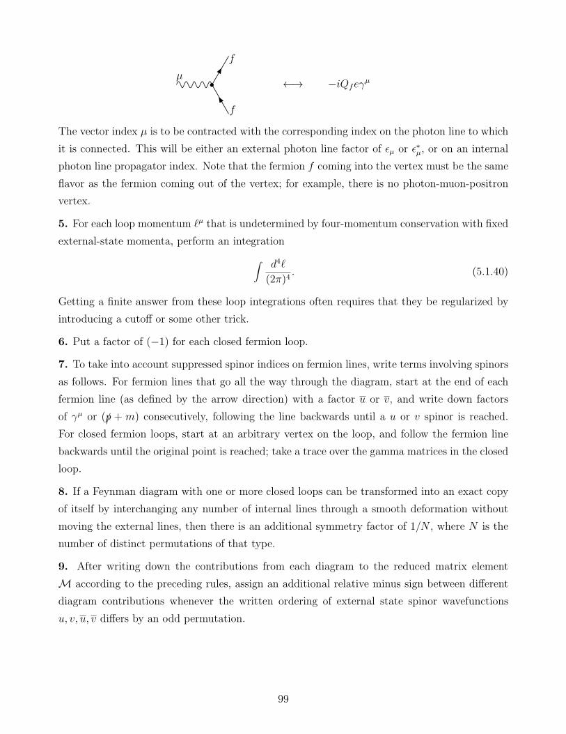
←→ −iQfeγµ

µ

f

f

The vector index µ is to be contracted with the corresponding index on the photon line to which

it is connected. This will be either an external photon line factor of ǫµ or ǫ∗µ, or on an internal

photon line propagator index. Note that the fermion f coming into the vertex must be the same

flavor as the fermion coming out of the vertex; for example, there is no photon-muon-positron

vertex.

5. For each loop momentum ℓµ that is undetermined by four-momentum conservation with fixed

external-state momenta, perform an integration

∫ d4ℓ

(2π)4. (5.1.40)

Getting a finite answer from these loop integrations often requires that they be regularized by

introducing a cutoff or some other trick.

6. Put a factor of (−1) for each closed fermion loop.

7. To take into account suppressed spinor indices on fermion lines, write terms involving spinors

as follows. For fermion lines that go all the way through the diagram, start at the end of each

fermion line (as defined by the arrow direction) with a factor u or v, and write down factors

of γµ or (/p + m) consecutively, following the line backwards until a u or v spinor is reached.

For closed fermion loops, start at an arbitrary vertex on the loop, and follow the fermion line

backwards until the original point is reached; take a trace over the gamma matrices in the closed

loop.

8. If a Feynman diagram with one or more closed loops can be transformed into an exact copy

of itself by interchanging any number of internal lines through a smooth deformation without

moving the external lines, then there is an additional symmetry factor of 1/N , where N is the

number of distinct permutations of that type.

9. After writing down the contributions from each diagram to the reduced matrix element

M according to the preceding rules, assign an additional relative minus sign between different

diagram contributions whenever the written ordering of external state spinor wavefunctions

u, v, u, v differs by an odd permutation.

99

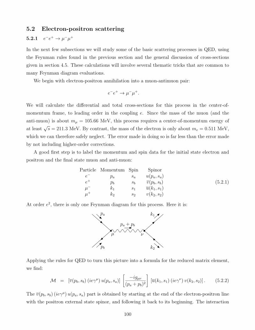
5.2 Electron-positron scattering

5.2.1 e−e+ → µ−µ+

In the next few subsections we will study some of the basic scattering processes in QED, using

the Feynman rules found in the previous section and the general discussion of cross-sections

given in section 4.5. These calculations will involve several thematic tricks that are common to

many Feynman diagram evaluations.

We begin with electron-positron annihilation into a muon-antimuon pair:

e−e+ → µ−µ+.

We will calculate the differential and total cross-sections for this process in the center-of-

momentum frame, to leading order in the coupling e. Since the mass of the muon (and the

anti-muon) is about mµ = 105.66 MeV, this process requires a center-of-momentum energy of

at least√s = 211.3 MeV. By contrast, the mass of the electron is only about me = 0.511 MeV,

which we can therefore safely neglect. The error made in doing so is far less than the error made

by not including higher-order corrections.

A good first step is to label the momentum and spin data for the initial state electron and

positron and the final state muon and anti-muon:

Particle Momentum Spin Spinore− pa sa u(pa, sa)e+ pb sb v(pb, sb)µ− k1 s1 u(k1, s1)µ+ k2 s2 v(k2, s2)

(5.2.1)

At order e2, there is only one Feynman diagram for this process. Here it is:

pa

µ ν

k1

pb k2

pa + pb

Applying the rules for QED to turn this picture into a formula for the reduced matrix element,

we find:

M = [v(pb, sb) (ieγµ) u(pa, sa)]

[−igµν

(pa + pb)2

][u(k1, s1) (ieγ

ν) v(k2, s2)] . (5.2.2)

The v(pb, sb) (ieγµ) u(pa, sa) part is obtained by starting at the end of the electron-positron line

with the positron external state spinor, and following it back to its beginning. The interaction

100

vertex is −iQeγµ = ieγµ, since the charge of the electron and muon is Q = −1. Likewise, the

u(k1, s1) (ieγν) v(k2, s2) part is obtained by starting at the end of the muon-antimuon line with

the muon external state spinor, and following it backwards. The photon propagator is written

in Feynman gauge, for simplicity, and carries indices µ and ν that connect to the two fermion

lines at their respective interaction vertices.

We can write this result more compactly by using abbreviations v(pb, sb) = vb and u(pa, sa) ≡ua, etc. Writing the denominator of the photon propagator as the Mandelstam variable s =

(pa + pb)2 = (k1 + k2)

2, and using the metric in the photon propagator to lower the index on

one of the gamma matrices, we get:

M = ie2

s(vbγµua)(u1γ

µv2). (5.2.3)

The differential cross-section involves the complex square ofM:

|M|2 =e4

s2(vbγµua)(u1γ

µv2)(vbγνua)∗(u1γ

νv2)∗. (5.2.4)

Evaluating the complex conjugated terms in parentheses can be done systematically by taking

the Hermitian conjugate of the Dirac spinors and matrices they are made of, taking care to write

them in the reverse order. So, for example,

(vbγνua)∗ = (v†bγ

0γνua)∗ = u†aγ

†νγ

0vb = u†aγ0γνvb = uaγνvb. (5.2.5)

The third equality follows from the identity (A.2.5), which implies γ†νγ0 = γ0γν . Similarly,

(u1γνv2)

∗ = v2γνu1. (5.2.6)

[Following the same strategy, one can show that in general,

(xγµγν . . . γρy)∗ = yγρ . . . γνγµx (5.2.7)

where x and y are any u and v spinors.] Therefore we have:

|M|2 = e4

s2(vbγµua)(uaγνvb) (u1γ

µv2)(v2γνu1). (5.2.8)

At this point, we could work out explicit forms for the external state spinors and plug

eq. (5.2.8) into eq. (4.5.47) to find the differential cross-section for any particular set of spins.

However, this is not very convenient, and fortunately it is not necessary either. In a real exper-

iment, the final state spins of the muon and anti-muon are typically not measured. Therefore,

to find the total cross-section for all possible final states, we should sum over s1 and s2. Also, if

the initial-state electron spin states are unknown, we should average over sa and sb. (One must

101

average, not sum, over the initial-state spins, because sa and sb cannot simultaneously take on

both spin-up and spin-down values; there is only one initial state, even if it is unknown.) These

spin sums and averages will allow us to exploit the identities (3.2.50) and (3.2.51) [also listed

in Appendix B as (A.2.29) and (A.2.30)], so that the explicit forms for the spinors are never

needed.

After doing the spin sum and average, the differential cross-section must be symmetric under

rotations about the collision axis. This is because the only special directions in the problem are

the momenta of the particles, so that the cross-section can only depend on the angle θ between

the collision axis determined by the two initial-state particles and the scattering axis determined

by the two final-state particles. So, we can apply eq. (4.5.48) to obtain:

dσ

d(cos θ)=

1

2

∑

sa

1

2

∑

sb

∑

s1

∑

s2

|M|2 |~k1|32πs|~pa|

(5.2.9)

in the center-of-momentum frame, with the effects of initial state spin averaging and final state

spin summing now included.

We can now use eqs. (A.2.29) and (A.2.30), which in the present situation imply

∑

sa

uaua = /pa +me, (5.2.10)

∑

s2

v2v2 = /k2 −mµ. (5.2.11)

Neglecting me as promised earlier, we obtain:

1

2

∑

sa

1

2

∑

sb

∑

s1

∑

s2

|M|2 =e4

4s2∑

sb

∑

s1

(vbγµ/paγνvb) (u1γµ[/k2 −mµ]γ

νu1). (5.2.12)

Now we apply another trick. A dot product of two vectors is equal to the trace of the vectors

multiplied in the opposite order to form a matrix:

( a1 a2 a3 a4 )

b1b2b3b4

= Tr

[

b1b2b3b4

( a1 a2 a3 a4 )

]≡ Tr

b1a1 b1a2 b1a3 b1a4b2a1 b2a2 b2a3 b2a4b3a1 b3a2 b3a3 b3a4b4a1 b4a2 b4a3 b4a4

.(5.2.13)

Applying this to each expression in parentheses in eq. (5.2.12), we move the barred spinor

(thought of as a row vector) to the end and take the trace over the resulting 4× 4 Dirac spinor

matrix. So:

vbγµ/paγνvb = Tr[γµ/paγνvbvb], (5.2.14)

u1γµ[/k2 −mµ]γ

νu1 = Tr[γµ(/k2 −mµ)γνu1u1], (5.2.15)

102

so that

1

4

∑

spins

|M|2 = e4

4s2∑

sb

∑

s1

Tr[γµ/paγνvbvb] Tr[γµ(/k2 −mµ)γ

νu1u1]. (5.2.16)

The reason this trick of rearranging into a trace is useful is that now we can once again exploit

the spin-sum identities (A.2.29) and (A.2.30), this time in the form:

∑

sb

vbvb = /pb −me, (5.2.17)

∑

s1

u1u1 = /k1 +mµ. (5.2.18)

The result, again neglecting me, is:

1

4

∑

spins

|M|2 = e4

4s2Tr[γµ/paγν/pb] Tr[γ

µ(/k2 −mµ)γν(/k1 +mµ)]. (5.2.19)

Next we must evaluate the traces. First,

Tr[γµ/paγν/pb] = pαapβbTr[γµγαγνγβ] (5.2.20)

= pαapβb (4gµαgνβ − 4gµνgαβ + 4gµβgνα) (5.2.21)

= 4paµpbν − 4gµνpa · pb + 4pbµpaν , (5.2.22)

where we have used the general result for the trace of four gamma matrices found in the home-

work, and listed in eq. (A.2.10). Similarly, making use of the fact that the trace of an odd

number of gamma matrices is zero:

Tr[γµ(/k2 −mµ)γν(/k1 +mµ)] = Tr[γµ/k2γ

ν/k1]−m2µTr[γ

µγν ] (5.2.23)

= 4kµ2kν1 − 4gµνk1 · k2 + 4kµ1k

ν2 − 4gµνm2

µ, (5.2.24)

where eqs. (A.2.8)-(A.2.10) have been used. Taking the product of the two traces, one finds

that the answer reduces to simply:

1

4

∑

spins

|M|2 = e4

s28[(pa · k2)(pb · k1) + (pa · k1)(pb · k2) + (pa · pb)m2

µ

]. (5.2.25)

Our next task is to work out the kinematic quantities appearing in eq. (5.2.25). Let us call P

and K the magnitudes of the 3-momenta of the electron and the muon, respectively. We assume

that the electron is initially moving in the +z direction, and the muon makes an angle θ with

respect to the positive z axis, within the yz plane. The on-shell conditions for the particles are:

p2a = p2b = m2e ≈ 0, (5.2.26)

k21 = k22 = m2µ. (5.2.27)

103

Then we have:

pa = (P, 0, 0, P ), (5.2.28)

pb = (P, 0, 0, −P ), (5.2.29)

k1 = (√K2 +m2

µ, 0, K sin θ, K cos θ), (5.2.30)

k2 = (√K2 +m2

µ, 0, −K sin θ, −K cos θ). (5.2.31)

Since (pa + pb)2 = (k1 + k2)

2 = s, it follows that

P =

√s

4, (5.2.32)

K =

√s

4−m2

µ, (5.2.33)

and

pa · pb = 2P 2 =s

2, (5.2.34)

pa · k1 = pb · k2 = P√K2 +m2

µ − PK cos θ =s

4

1− cos θ

√

1− 4m2µ

s

, (5.2.35)

pa · k2 = pb · k1 = P√K2 +m2

µ + PK cos θ =s

4

1 + cos θ

√

1− 4m2µ

s

. (5.2.36)

Putting these results into eq. (5.2.25), we get:

1

4

∑

spins

|M|2 =8e4

s2

(s

4

)2[1 + cos θ

√

1− 4m2µ

s

]2+(s

4

)2[1− cos θ

√

1− 4m2µ

s

]2+sm2

µ

2

= e4[1 +

4m2µ

s+

(1− 4m2

µ

s

)cos2 θ

]. (5.2.37)

Finally we can plug this into eq. (5.2.9):

dσ

d(cos θ)=

1

4

∑

spins

|M|2 K

32πsP(5.2.38)

=e4

32πs

√

1− 4m2µ

s

[1 +

4m2µ

s+

(1− 4m2

µ

s

)cos2 θ

], (5.2.39)

or, rewriting in terms of the fine structure constant α = e2/4π,

dσ

d(cos θ)=

πα2

2s

√

1− 4m2µ

s

[1 +

4m2µ

s+

(1− 4m2

µ

s

)cos2 θ

]. (5.2.40)

Doing the integral over cos θ using∫ 1−1 d(cos θ) = 2 and

∫ 1−1 cos

2 θ d(cos θ) = 2/3, we find the

total cross-section:

σ =4πα2

3s

√

1− 4m2µ

s

(1 +

2m2µ

s

). (5.2.41)

104

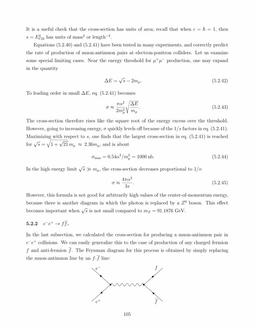
It is a useful check that the cross-section has units of area; recall that when c = h = 1, then

s = E2CM has units of mass2 or length−2.

Equations (5.2.40) and (5.2.41) have been tested in many experiments, and correctly predict

the rate of production of muon-antimuon pairs at electron-positron colliders. Let us examine

some special limiting cases. Near the energy threshold for µ+µ− production, one may expand

in the quantity

∆E =√s− 2mµ. (5.2.42)

To leading order in small ∆E, eq. (5.2.41) becomes

σ ≈ πα2

2m2µ

√∆E

mµ

. (5.2.43)

The cross-section therefore rises like the square root of the energy excess over the threshold.

However, going to increasing energy, σ quickly levels off because of the 1/s factors in eq. (5.2.41).

Maximizing with respect to s, one finds that the largest cross-section in eq. (5.2.41) is reached

for√s =

√1 +√21mµ ≈ 2.36mµ, and is about

σmax = 0.54α2/m2µ = 1000 nb. (5.2.44)

In the high energy limit√s≫ mµ, the cross-section decreases proportional to 1/s:

σ ≈ 4πα2

3s. (5.2.45)

However, this formula is not good for arbitrarily high values of the center-of-momentum energy,

because there is another diagram in which the photon is replaced by a Z0 boson. This effect

becomes important when√s is not small compared to mZ = 91.1876 GeV.

5.2.2 e−e+ → ff .

In the last subsection, we calculated the cross-section for producing a muon-antimuon pair in

e−e+ collisions. We can easily generalize this to the case of production of any charged fermion

f and anti-fermion f . The Feynman diagram for this process is obtained by simply replacing

the muon-antimuon line by an f -f line:

e− f

e+ f

105

The reduced matrix element for this process has exactly the same form as for e−e+ → ff , except

that the photon-µ−-µ+ vertex is replaced by a photon-f -f vertex, with:

ieγν −→ −iQfeγν , (5.2.46)

where Qf is the charge of the fermion f . In the case of quarks, there are three indistinguishable

colors for each flavor (up, down, strange, charm, bottom, top). The photon-quark-antiquark

vertex is diagonal in color, so the three colors are simply summed over in order to find the total

cross-section for a given flavor. In general, if we call nf the number of colors (or perhaps other

non-spin degrees of freedom) of the fermion f , then we have:

|Me−e+→ff |2 = nfQ2f |Me−e+→µ−µ+ |2, (5.2.47)

where it is understood that mµ should be replaced by mf everywhere in |Me−e+→ff |2. It followsthat the differential and total cross-sections for e−e+ → ff are obtained from eqs. (5.2.40) and

(5.2.41) by just multiplying by nfQ2f and replacing mµ → mf :

σe−e+→ff = nfQ2f

4πα2

3s

√

1− 4m2f

s

(1 +

2m2f

s

). (5.2.48)

In the high-energy limit√s≫ mf , we have:

σe−e+→ff = nfQ2f

4πα2

3s. (5.2.49)

The following graph compares the total cross-section for e+e− → ff (solid line) as given by

eq. (5.2.48) to the asymptotic approximation (dashed line) given by eq. (5.2.49).

0 1 2 3 4 5E

CM/m

f

0

0.54 nfQ

f

2α2/m

f

2

σ

106

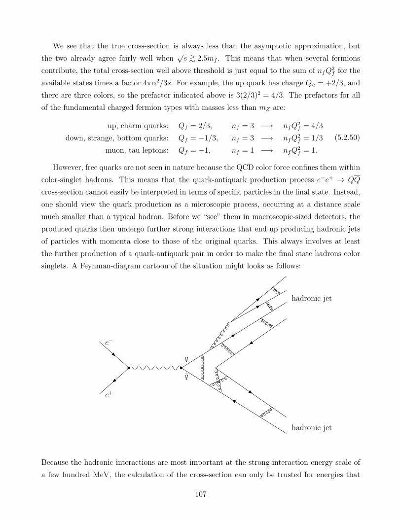
We see that the true cross-section is always less than the asymptotic approximation, but

the two already agree fairly well when√s >∼ 2.5mf . This means that when several fermions

contribute, the total cross-section well above threshold is just equal to the sum of nfQ2f for the

available states times a factor 4πα2/3s. For example, the up quark has charge Qu = +2/3, and

there are three colors, so the prefactor indicated above is 3(2/3)2 = 4/3. The prefactors for all

of the fundamental charged fermion types with masses less than mZ are:

up, charm quarks: Qf = 2/3, nf = 3 −→ nfQ2f = 4/3

down, strange, bottom quarks: Qf = −1/3, nf = 3 −→ nfQ2f = 1/3

muon, tau leptons: Qf = −1, nf = 1 −→ nfQ2f = 1.

(5.2.50)

However, free quarks are not seen in nature because the QCD color force confines them within

color-singlet hadrons. This means that the quark-antiquark production process e−e+ → QQ

cross-section cannot easily be interpreted in terms of specific particles in the final state. Instead,

one should view the quark production as a microscopic process, occurring at a distance scale

much smaller than a typical hadron. Before we “see” them in macroscopic-sized detectors, the

produced quarks then undergo further strong interactions that end up producing hadronic jets

of particles with momenta close to those of the original quarks. This always involves at least

the further production of a quark-antiquark pair in order to make the final state hadrons color

singlets. A Feynman-diagram cartoon of the situation might looks as follows:

e−

e+

q

q

hadronic jet

hadronic jet

Because the hadronic interactions are most important at the strong-interaction energy scale of

a few hundred MeV, the calculation of the cross-section can only be trusted for energies that

107

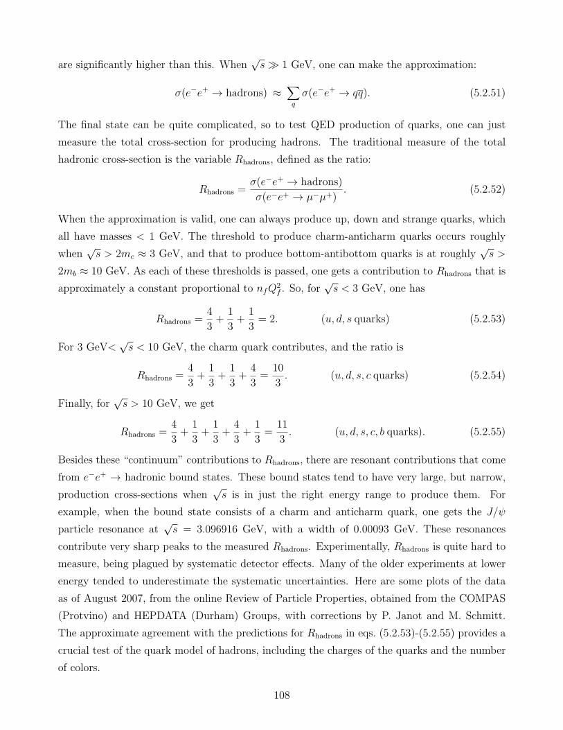
are significantly higher than this. When√s≫ 1 GeV, one can make the approximation:

σ(e−e+ → hadrons) ≈∑

q

σ(e−e+ → qq). (5.2.51)

The final state can be quite complicated, so to test QED production of quarks, one can just

measure the total cross-section for producing hadrons. The traditional measure of the total

hadronic cross-section is the variable Rhadrons, defined as the ratio:

Rhadrons =σ(e−e+ → hadrons)

σ(e−e+ → µ−µ+). (5.2.52)

When the approximation is valid, one can always produce up, down and strange quarks, which

all have masses < 1 GeV. The threshold to produce charm-anticharm quarks occurs roughly

when√s > 2mc ≈ 3 GeV, and that to produce bottom-antibottom quarks is at roughly

√s >

2mb ≈ 10 GeV. As each of these thresholds is passed, one gets a contribution to Rhadrons that is

approximately a constant proportional to nfQ2f . So, for

√s < 3 GeV, one has

Rhadrons =4

3+

1

3+

1

3= 2. (u, d, s quarks) (5.2.53)

For 3 GeV<√s < 10 GeV, the charm quark contributes, and the ratio is

Rhadrons =4

3+

1

3+

1

3+

4

3=

10

3. (u, d, s, c quarks) (5.2.54)

Finally, for√s > 10 GeV, we get

Rhadrons =4

3+

1

3+

1

3+

4

3+

1

3=

11

3. (u, d, s, c, b quarks). (5.2.55)

Besides these “continuum” contributions to Rhadrons, there are resonant contributions that come

from e−e+ → hadronic bound states. These bound states tend to have very large, but narrow,

production cross-sections when√s is in just the right energy range to produce them. For

example, when the bound state consists of a charm and anticharm quark, one gets the J/ψ

particle resonance at√s = 3.096916 GeV, with a width of 0.00093 GeV. These resonances

contribute very sharp peaks to the measured Rhadrons. Experimentally, Rhadrons is quite hard to

measure, being plagued by systematic detector effects. Many of the older experiments at lower

energy tended to underestimate the systematic uncertainties. Here are some plots of the data

as of August 2007, from the online Review of Particle Properties, obtained from the COMPAS

(Protvino) and HEPDATA (Durham) Groups, with corrections by P. Janot and M. Schmitt.

The approximate agreement with the predictions for Rhadrons in eqs. (5.2.53)-(5.2.55) provides a

crucial test of the quark model of hadrons, including the charges of the quarks and the number

of colors.

108

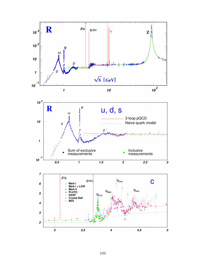
10-1

1

10

102

103

1 10 102

ρ

ωφ

ρ

J/ψ ψ(2S)ZR

S GeV

10-1

1

10

102

0.5 1 1.5 2 2.5 3

3-loop pQCD

Naive quark model

Sum of exclusivemeasurements

Inclusivemeasurements

R

ρ

ω

φ

ρ

u, d, s

2

3

4

5

6

7

3 3.5 4 4.5 5

Mark IMark I + LGWMark IIPLUTODASPCrystal BallBES

J/ψψ(2S)

ψ3770

ψ4040

ψ4160

ψ4415

c

109

2

3

4

5

6

7

8

9.5 10 10.5 11

ARGUSCrystal BallCLEO

CLEO IICUSBDASP

DHHMLENAMD-1

(1S)

(2S)

(3S)

(4S)

b

S GeV

5.2.3 Helicities in e−e+ → µ−µ+

Up to now, we have computed the cross-section by averaging over the unknown spins of the initial

state electron and positron. However, some e−e+ colliders can control the initial spin states,

using polarized beams. This means that the beams are arranged to have an excess of either

L-handed or R-handed helicity electrons and positrons. Practical realities make it impossible to

achieve 100%-pure polarized beams, of course. At a proposed future Linear Collider, it is a very

important part of the experimental program to be able to run with at least the electron beam

polarized. Present estimates are that one might be able to get 90% or 95% pure polarization

for the electron beam (either L or R), with perhaps 60% polarization for the positron beam.

This terminology means that when the beam is operating in R mode, then a polarization of X%

implies that

PR − PL = X% (5.2.56)

where PR and PL are the probabilities of measuring the spin pointing along and against the 3-

momentum direction, respectively. This experimental capability shows that one needs to be able

to calculate cross-sections without assuming that the initial spin state is random and averaged

over.

We could redo the calculation of the previous subsections with particular spinors u(p, s) and

v(p, s) for the desired specific spin states s of initial state particles. However, then we would lose

our precious trick of evaluating∑

s uu and∑

s vv. A nicer way is to keep the sum over spins, but

eliminate the “wrong” polarization from the sum using a projection matrix from eq. (3.2.30).

So, for example, we can use

PLu(p, s) ←→ L initial-state particle, (5.2.57)

110

PRu(p, s) ←→ R initial-state particle, (5.2.58)

in place of the usual Feynman rules for an initial state particle. Summing over the spin s will not

change the fact that the projection matrix allows only L- or R-handed electrons to contribute to

the cross-section. Now our traces over gamma matrices will involve γ5, because of the explicit

expressions for PL and PR [see eq. (3.2.30)].

To get the equivalent rules for an initial state antiparticle, we must remember that the spin

operator acting on v(p, s) spinors is the opposite of the spin operator acting on u(p, s) spinors.

Therefore, PL acting on a v(p, s) spinor projects onto a R-handed antiparticle. So if we form the

object v(p, s)PR = v†(p, s)γ0PR = v†(p, s)PLγ0, the result must describe a R-handed positron;

in this case, the bar on the spinor for an antiparticle “corrects” the handedness. So, for an

initial state antiparticle with either L or R polarization, we can use:

v(p, s)PL ←→ L initial-state anti-particle, (5.2.59)

v(p, s)PR ←→ R initial-state anti-particle. (5.2.60)

In some cases, one can also measure the polarizations of outgoing particles, for example by

observing their decays. Tau leptons and anti-taus sometimes decay by the weak interaction

processes:

τ− → ℓ−ντνℓ (5.2.61)

, τ+ → ℓ+ντνℓ, (5.2.62)

where ℓ is either e or µ, with the angular distributions of the final state directions depending on

the spin of the τ , which may be one of the final state fermions in a scattering or decay process

of interest. If the polarization of a final-state fermion is fixed by measurement, then we need to

use:

u(p, s)PR ←→ L final-state particle, (5.2.63)

u(p, s)PL ←→ R final-state particle, (5.2.64)

PRv(p, s) ←→ L final-state anti-particle, (5.2.65)

PLv(p, s) ←→ R final-state anti-particle, (5.2.66)

in order to be able to calculate cross-sections to final states with specific L or R spin polarization

states. (As a result of the barred spinor notation, the general rule is that the projection matrix

in an initial state has the same handedness as the incoming particle or antiparticle, while the

projection matrix in a final state has the opposite handedness of the particle being produced.)

111

As an example, let us consider the process:

e−Re+R → µ−µ+, (5.2.67)

where the helicities of the initial state particles are now assumed to be known perfectly. The

reduced matrix element for this process, following from the same Feynman diagram as before,

is:

M = ie2

s(vbPRγ

µPRua) (u2γµv1). (5.2.68)

As you should have discovered in a homework problem, a projection matrix can be moved

through a gamma matrix by changing L↔ R:

PRγµ = γµPL, (5.2.69)

PLγµ = γµPR. (5.2.70)

This follows from the fact that γ5 anticommutes with γµ:

PRγµ =

(1 + γ5

2

)γµ = γµ

(1− γ5

2

)= γµPL. (5.2.71)

Therefore, eq. (5.2.68) simply vanishes, because

PRγµPR = γµPLPR = 0. (5.2.72)

Therefore, the process e−Re+R → µ−µ+ does not occur in QED. Similarly, e−Le

+L → µ−µ+ does not

occur in QED. By the same type of argument, µ− and µ+ in the final state must have opposite

L,R polarizations from each other in QED.

To study a non-vanishing reduced matrix element, let us therefore consider the process:

e−Le+R → µ−

Lµ+R, (5.2.73)

in which we have now assumed that all helicities are perfectly known. To simplify matters,

we will assume the high energy limit√s ≫ mµ. The reduced matrix element can be simply

obtained from eq. (5.2.3) by just putting in the appropriate L and R projection matrices acting

on each external state spinor:

M = ie2

s(vbPRγ

µPLua)(u1PRγµPLv2). (5.2.74)

This can be simplified slightly by using the properties of the projections matrices:

PRγµPL = γµPLPL = γµPL, (5.2.75)

112

so that

M = ie2

s(vbγ

µPLua)(u1γµPLv2), (5.2.76)

and so

|M|2 =e4

s2(vbγ

µPLua)(u1γµPLv2)(vbγνPLua)

∗(u1γνPLv2)∗. (5.2.77)

To evaluate this, we compute:

(vbγνPLua)

∗ = (v†bγ0γνPLua)

∗ = u†a(PL)†(γν)†γ0vb (5.2.78)

= u†aPLγ0γνvb (5.2.79)

= u†aγ0PRγ

νvb (5.2.80)

= uaPRγνvb. (5.2.81)

Here we have used the facts that (PL)† = PL, and (γν)†γ0 = γ0γν , and PLγ

0 = γ0PR, and

u†aγ0 = ua. In a similar way,

(u1γνPLv2)∗ = v2PRγνu1. (5.2.82)

Therefore,

|M|2 = e4

s2(vbγ

µPLua)(uaPRγνvb)(u1γµPLv2)(v2PRγνu1). (5.2.83)

Because the spin projection matrices will only allow the specified set of spins to contribute

anyway, we are free to sum over the spin labels sa, sb, s1, and s2, without changing anything.

Let us do so, since it will allow us to apply the tricks

∑

sa

uaua = /pa +me, (5.2.84)

∑

s2

v2v2 = /k2 −mµ. (5.2.85)

Neglecting the masses because of the high-energy limit, we therefore have

|M|2 =∑

sa

∑

sb

∑

s1

∑

s2

|M|2 (5.2.86)

=e4

s2∑

s1

∑

sb

(vbγµPL/paPRγ

νvb) (u1γµPL/k2PRγνu1). (5.2.87)

This can be simplified by eliminating excess projection matrices, using:

PL/paPR = /paPRPR = /paPR, (5.2.88)

PL/k2PR = /k2PRPR = /k2PR, (5.2.89)

113

to get

|M|2 = e4

s2∑

s1

∑

sb

(vbγµ/paPRγ

νvb) (u1γµ/k2PRγνu1). (5.2.90)

Again using the trick of putting the barred spinor at the end and taking the trace [see the

discussion around eq. (5.2.13)] for each quantity in parentheses, this becomes:

|M|2 = e4

s2∑

s1

∑

sb

Tr[γµ/paPRγνvbvb] Tr[γµ/k2PRγνu1u1]. (5.2.91)

Doing the sums over s1 and sb using the usual trick gives:

|M|2 = e4

s2Tr[γµ/paPRγ

ν/pb] Tr[γµ/k2PRγν/k1]. (5.2.92)

Now it is time to evaluate the traces. We have

Tr[γµ/paPRγν/pb] = Tr[γµ/pa

(1 + γ5

2

)γν/pb] (5.2.93)

=1

2Tr[γµ/paγ

ν/pb] +

1

2Tr[γµ/paγ

ν/pbγ5], (5.2.94)

where we have used the fact that γ5 anticommutes with any gamma matrix to rearrange the

order in the last term. The first of these traces was evaluated in section 5.2.1. The trace

involving γ5 is, from eq. (A.2.19):

Tr[γµ/paγν/pbγ5] = paαpbβTr[γ

µγαγνγβγ5] (5.2.95)

= paαpbβ(4iǫµανβ). (5.2.96)

where ǫµανβ is the totally antisymmetric Levi-Civita tensor defined in eq. (2.3.21). Putting

things together:

Tr[γµ/paPRγν/pb] = 2

[pµap

νb − gµν(pa · pb) + pµb p

νa + ipaαpbβǫ

µανβ]. (5.2.97)

In exactly the same way, we get

Tr[γµ/k2PRγν/k1] = 2 [k2µk1ν − gµν(k2 · k1) + k1µk2ν + ikρ2kσ1 ǫµρνσ] . (5.2.98)

Finally, we have to multiply these two traces together, contracting the indices µ and ν. Note

that the cross-terms containing only one ǫ tensor vanish, because the epsilon tensors are anti-

symmetric under µ↔ ν, while the other terms are symmetric. The term involving two epsilon

tensors can be evaluated using the useful identity

ǫµανβǫµρνσ = −2δαρ δβσ + 2δασδβρ , (5.2.99)

114

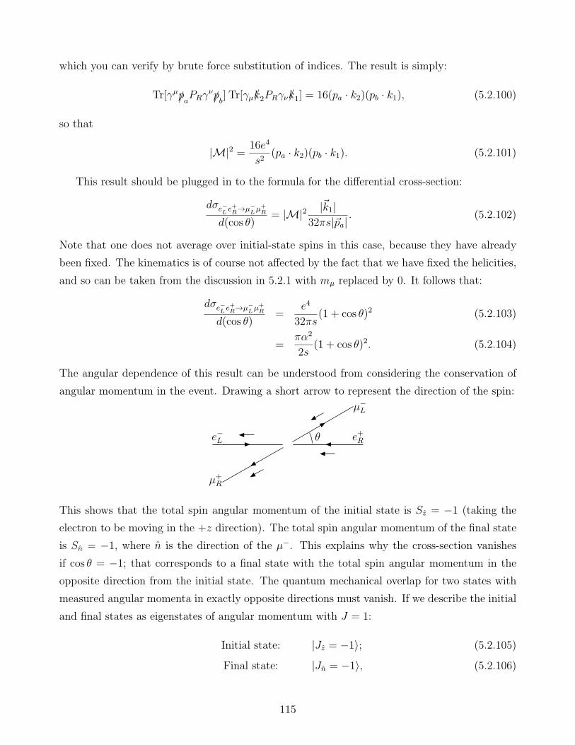
which you can verify by brute force substitution of indices. The result is simply:

Tr[γµ/paPRγν/pb] Tr[γµ/k2PRγν/k1] = 16(pa · k2)(pb · k1), (5.2.100)

so that

|M|2 = 16e4

s2(pa · k2)(pb · k1). (5.2.101)

This result should be plugged in to the formula for the differential cross-section:

dσe−Le+R→µ−

Lµ+

R

d(cos θ)= |M|2 |~k1|

32πs|~pa|. (5.2.102)

Note that one does not average over initial-state spins in this case, because they have already

been fixed. The kinematics is of course not affected by the fact that we have fixed the helicities,

and so can be taken from the discussion in 5.2.1 with mµ replaced by 0. It follows that:

dσe−Le+R→µ−

Lµ+

R

d(cos θ)=

e4

32πs(1 + cos θ)2 (5.2.103)

=πα2

2s(1 + cos θ)2. (5.2.104)

The angular dependence of this result can be understood from considering the conservation of

angular momentum in the event. Drawing a short arrow to represent the direction of the spin:

e−L e+R

µ+R

µ−L

θ

This shows that the total spin angular momentum of the initial state is Sz = −1 (taking the

electron to be moving in the +z direction). The total spin angular momentum of the final state

is Sn = −1, where n is the direction of the µ−. This explains why the cross-section vanishes

if cos θ = −1; that corresponds to a final state with the total spin angular momentum in the

opposite direction from the initial state. The quantum mechanical overlap for two states with

measured angular momenta in exactly opposite directions must vanish. If we describe the initial

and final states as eigenstates of angular momentum with J = 1:

Initial state: |Jz = −1〉; (5.2.105)

Final state: |Jn = −1〉, (5.2.106)

115

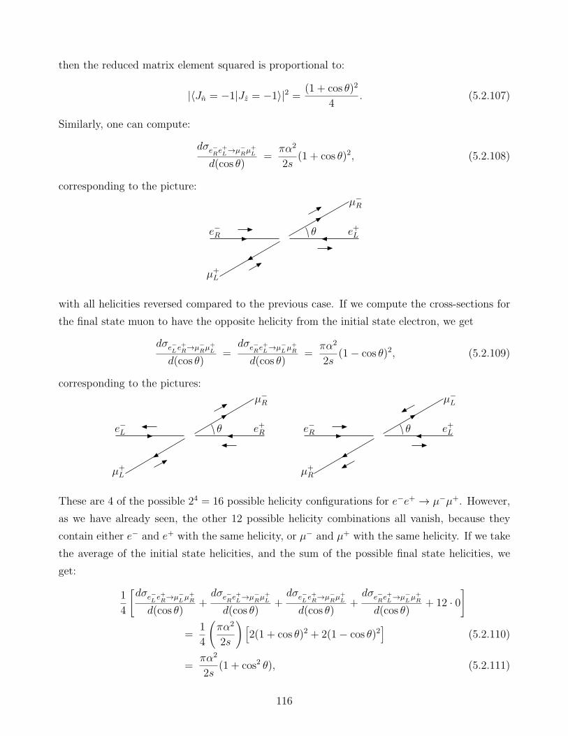
then the reduced matrix element squared is proportional to:

|〈Jn = −1|Jz = −1〉|2 =(1 + cos θ)2

4. (5.2.107)

Similarly, one can compute:

dσe−Re+L→µ−

Rµ+

L

d(cos θ)=

πα2

2s(1 + cos θ)2, (5.2.108)

corresponding to the picture:

e−R e+L

µ+L

µ−R

θ

with all helicities reversed compared to the previous case. If we compute the cross-sections for

the final state muon to have the opposite helicity from the initial state electron, we get

dσe−Le+R→µ−

Rµ+

L

d(cos θ)=

dσe−Re+L→µ−

Lµ+

R

d(cos θ)=

πα2

2s(1− cos θ)2, (5.2.109)

corresponding to the pictures:

e−L e+R

µ+L

µ−R

θ e−R e+L

µ+R

µ−L

θ

These are 4 of the possible 24 = 16 possible helicity configurations for e−e+ → µ−µ+. However,

as we have already seen, the other 12 possible helicity combinations all vanish, because they

contain either e− and e+ with the same helicity, or µ− and µ+ with the same helicity. If we take

the average of the initial state helicities, and the sum of the possible final state helicities, we

get:

1

4

[dσe−

Le+R→µ−

Lµ+

R

d(cos θ)+dσe−

Re+L→µ−

Rµ+

L

d(cos θ)+dσe−

Le+R→µ−

Rµ+

L

d(cos θ)+dσe−

Re+L→µ−

Lµ+

R

d(cos θ)+ 12 · 0

]

=1

4

(πα2

2s

) [2(1 + cos θ)2 + 2(1− cos θ)2

](5.2.110)

=πα2

2s(1 + cos2 θ), (5.2.111)

116

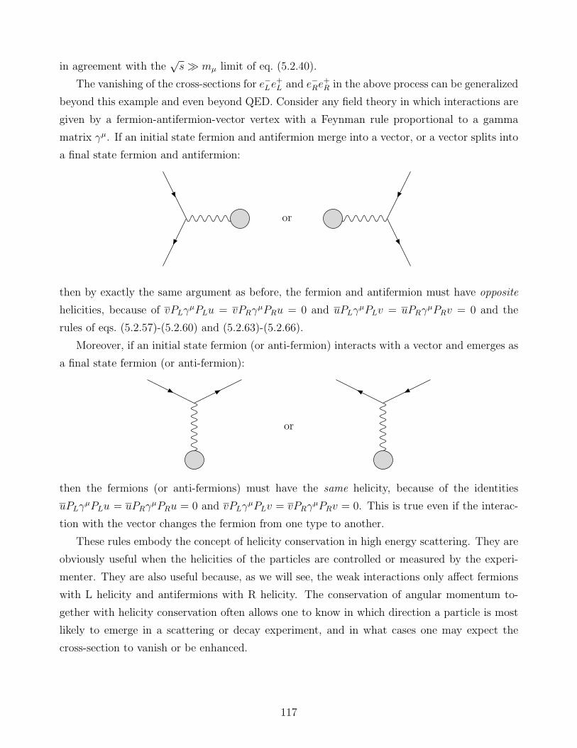
in agreement with the√s≫ mµ limit of eq. (5.2.40).

The vanishing of the cross-sections for e−Le+L and e−Re

+R in the above process can be generalized

beyond this example and even beyond QED. Consider any field theory in which interactions are

given by a fermion-antifermion-vector vertex with a Feynman rule proportional to a gamma

matrix γµ. If an initial state fermion and antifermion merge into a vector, or a vector splits into

a final state fermion and antifermion:

or

then by exactly the same argument as before, the fermion and antifermion must have opposite

helicities, because of vPLγµPLu = vPRγ

µPRu = 0 and uPLγµPLv = uPRγ

µPRv = 0 and the

rules of eqs. (5.2.57)-(5.2.60) and (5.2.63)-(5.2.66).

Moreover, if an initial state fermion (or anti-fermion) interacts with a vector and emerges as

a final state fermion (or anti-fermion):

or

then the fermions (or anti-fermions) must have the same helicity, because of the identities

uPLγµPLu = uPRγ

µPRu = 0 and vPLγµPLv = vPRγ

µPRv = 0. This is true even if the interac-

tion with the vector changes the fermion from one type to another.

These rules embody the concept of helicity conservation in high energy scattering. They are

obviously useful when the helicities of the particles are controlled or measured by the experi-

menter. They are also useful because, as we will see, the weak interactions only affect fermions

with L helicity and antifermions with R helicity. The conservation of angular momentum to-

gether with helicity conservation often allows one to know in which direction a particle is most

likely to emerge in a scattering or decay experiment, and in what cases one may expect the

cross-section to vanish or be enhanced.

117

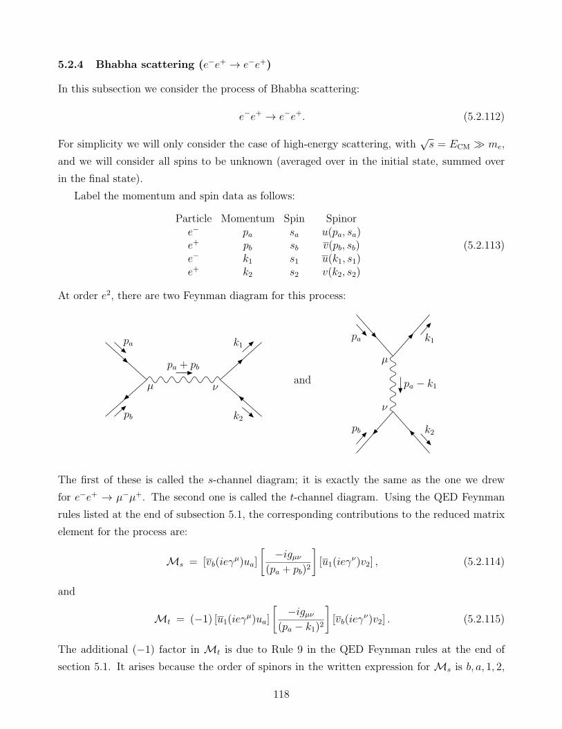
5.2.4 Bhabha scattering (e−e+ → e−e+)

In this subsection we consider the process of Bhabha scattering:

e−e+ → e−e+. (5.2.112)

For simplicity we will only consider the case of high-energy scattering, with√s = ECM ≫ me,

and we will consider all spins to be unknown (averaged over in the initial state, summed over

in the final state).

Label the momentum and spin data as follows:

Particle Momentum Spin Spinore− pa sa u(pa, sa)e+ pb sb v(pb, sb)e− k1 s1 u(k1, s1)e+ k2 s2 v(k2, s2)

(5.2.113)

At order e2, there are two Feynman diagram for this process:

pa

µ ν

k1

pb k2

pa + pb

and

k2

ν

µ

k1

pb

pa

pa − k1

The first of these is called the s-channel diagram; it is exactly the same as the one we drew

for e−e+ → µ−µ+. The second one is called the t-channel diagram. Using the QED Feynman

rules listed at the end of subsection 5.1, the corresponding contributions to the reduced matrix

element for the process are:

Ms = [vb(ieγµ)ua]

[−igµν

(pa + pb)2

][u1(ieγ

ν)v2] , (5.2.114)

and

Mt = (−1) [u1(ieγµ)ua][−igµν

(pa − k1)2][vb(ieγ

ν)v2] . (5.2.115)

The additional (−1) factor in Mt is due to Rule 9 in the QED Feynman rules at the end of

section 5.1. It arises because the order of spinors in the written expression forMs is b, a, 1, 2,

118

but that inMt is 1, a, b, 2, and these differ from each other by an odd permutation. We could

have just as well assigned the minus sign toMs instead; only the relative phases of terms in the

matrix element are significant.

Therefore the full reduced matrix element for Bhabha scattering, written in terms of the

Mandelstam variables s = (pa + pb)2 and t = (pa − k1)2, is:

M = Ms +Mt = ie21

s(vbγµua)(u1γ

µv2)−1

t(u1γµua)(vbγ

µv2). (5.2.116)

Taking the complex conjugate of this gives:

M∗ = M∗s +M∗

t (5.2.117)

= −ie21

s(vbγνua)

∗(u1γνv2)

∗ − 1

t(u1γνua)

∗(vbγνv2)

∗

(5.2.118)

= −ie21

s(uaγνvb)(v2γ

νu1)−1

t(uaγνu1)(v2γ

νvb). (5.2.119)

The complex square of the reduced matrix element, |M|2 =M∗M, contains a pure s-channel

piece proportional to 1/s2, a pure t-channel piece proportional to 1/t2, and an interference piece

proportional to 1/st. For organizational purposes, it is useful to calculate these pieces separately.

The pure s-channel contribution calculation is exactly the same as what we did before for

e−e+ → µ−µ+, except that now we can substitute mµ → me → 0. Therefore, plagiarizing the

result of eq. (5.2.25), we have:

1

4

∑

spins

|Ms|2 =8e4

s2[(pa · k2)(pb · k1) + (pa · k1)(pb · k2)] . (5.2.120)

The pure t-channel contribution can be calculated in a very similar way. We have:

|Mt|2 =e4

t2(v2γνvb)(vbγµv2)(u1γ

µua)(uaγνu1). (5.2.121)

Taking the average of initial state spins and the sum over final state spins allows us to use the

identities∑

sa uaua = /pa and∑

sa vbvb = /pb (neglecting me). The result is:

1

4

∑

spins

|Mt|2 =e4

4t2∑

s1,s2

(v2γν/pbγµv2)(u1γµ/paγ

νu1) (5.2.122)

=e4

4t2∑

s1,s2

Tr[γν/pbγµv2v2]Tr[γµ/paγ

νu1u1], (5.2.123)

in which we have turned the quantity into a trace by moving the u1 to the end. Now performing

the sums over s1, s2 gives:

1

4

∑

spins

|Mt|2 =e4

4t2Tr[γν/pbγµ/k2]Tr[γ

µ/paγ

ν/k1] (5.2.124)

=e4

4t2Tr[γµ/k2γν/pb]Tr[γ

µ/paγ

ν/k1]. (5.2.125)

119

In the second line, the first trace has been rearranged using the cyclic property of traces. The

point of doing so is that now these traces have exactly the same form that we encountered in

eq. (5.2.19), but with pa ↔ k2 and mµ → 0. Therefore we can obtain 14

∑spins |Mt|2 by simply

making the same replacements pa ↔ k2 and mµ → 0 in eq. (5.2.25):

1

4

∑

spins

|Mt|2 =8e4

t2[(pa · k2)(pb · k1) + (k2 · k1)(pb · pa)] . (5.2.126)

Next, consider the interference term:

1

4

∑

spins

M∗tMs = − e4

4st

∑

spins

(vbγµua)(uaγνu1)(u1γ

µv2)(v2γνvb). (5.2.127)

We chose to write the factors parentheses in that order, so that now we can immediately use

the tricks∑

sa uaua = /pa, and∑

s1 u1u1 = /k1, and∑

s2 v2v2 = /k2, to obtain:

1

4

∑

spins

M∗tMs = − e4

4st

∑

sb

(vbγµ/paγν/k1γ

µ/k2γνvb), (5.2.128)

which can now be converted into a trace by the usual trick of moving the vb to the end:

1

4

∑

spins

M∗tMs = − e4

4st

∑

sb

Tr[γµ/paγν/k1γ

µ/k2γνvbvb] (5.2.129)

= − e4

4stTr[γµ/paγ

ν/k1γµ/k2γν/pb]. (5.2.130)

Now we are faced with the task of computing the trace of 8 gamma matrices. In principle, the

trace of any number of gamma matrices can be performed with the algorithm of eq. (A.2.11).

The procedure is to replace the trace over 2n gamma matrices by a sum over traces of 2n − 2

gamma matrices, and repeat until all traces are short enough to evaluate using eqs. (A.2.8)-

(A.2.11) and (A.2.15)-(A.2.19). However, in many cases including the present one it is easier

to simplify the contents of the trace first, using eqs. (A.2.20)-(A.2.23). To evaluate the trace in

eq. (5.2.130), we first use eq. (A.2.23) to write:

γµ/paγν/k1γ

µ = −2/k1γν/pa, (5.2.131)

which implies that

Tr[γµ/paγν/k1γ

µ/k2γν/pb] = −2Tr[/k1γν/pa/k2γν/pb]. (5.2.132)

This can be further simplified by now using eq. (A.2.22) to write:

γν/pa/k2γν = 4pa · k2, (5.2.133)

120

so that:

Tr[γµ/paγν/k1γ

µ/k2γν/pb] = −8(pa · k2)Tr[/k1/pb] (5.2.134)

= −32(pa · k2)(k1 · pb), (5.2.135)

in which the trace has finally been performed using eq. (A.2.9). So, from eq. (5.2.130)

1

4

∑

spins

M∗tMs =

8e4

st(pa · k2)(pb · k1). (5.2.136)

Taking the complex conjugate of both sides, we also have:

1

4

∑

spins

M∗sMt =

8e4

st(pa · k2)(pb · k1). (5.2.137)

This completes the contributions to the total

1

4

∑

spins

|M|2 = 1

4

∑

spins

[|Ms|2 + |Mt|2 +M∗

tMs +M∗sMt

]. (5.2.138)

It remains to identify the dot products of momenta appearing in the above formulas. This

can be done by carrying over the kinematic analysis for the case e−e+ → µ−µ+ as worked out

in eqs. (5.2.26)-(5.2.36), with mµ,me → 0. Letting θ be the angle between the 3-momenta

directions of the initial state electron and the final state electron, we have:

pa · pb = k1 · k2 = s/2, (5.2.139)

pa · k1 = pb · k2 = −t/2, (5.2.140)

pa · k2 = pb · k1 = −u/2, (5.2.141)

with

t = −s2(1− cos θ), (5.2.142)

u = −s2(1 + cos θ). (5.2.143)

It follows from eqs. (5.2.120), (5.2.126), (5.2.136), and (5.2.137) that:

1

4

∑

spins

|Ms|2 =2e4

s2(u2 + t2) (5.2.144)

1

4

∑

spins

|Mt|2 =2e4

t2(u2 + s2) (5.2.145)

1

4

∑

spins

(M∗tMs +M∗

sMt) =4e4

stu2. (5.2.146)

121

Putting this into eq. (4.5.49), since |~pa| = |~k1|, we obtain the spin-averaged differential

cross-section for Bhabha scattering:

dσ

d(cos θ)=

e4

16πs

(u2 + t2

s2+u2 + s2

t2+

2u2

st

)(5.2.147)

=πα2

2s

(3 + cos2 θ

1− cos θ

)2

. (5.2.148)

This result actually diverges for cos θ → 1, because of the t’s in the denominator. This is

not an integrable singularity, because the differential cross-section blows up quadratically near

cos θ = 1, so

σ =∫ 1

−1

dσ

d(cos θ)d(cos θ) −→ ∞. (5.2.149)

The infinite total cross-section corresponds to the infinite range of the Coulomb potential be-

tween two charged particles. It arises entirely from the t-channel diagram, in which the electron

and positron scatter off of each other in the forward direction (θ ≈ 0). It simply reflects that

an infinite-range interaction will always produce some deflection, although it may be extremely

small. This result is the relativistic generalization of the non-relativistic, classical Rutherford

scattering problem, in which an electron or alpha particle (or some other light charged particle)

scatters off of the classical electric field of a heavy nucleus. As worked out in many textbooks on

classical physics (for example, H. Goldstein’s Classical Mechanics, J.D. Jackson’s Classical Elec-

trodynamics), the differential cross-section for a non-relativistic light particle with charge QA

and a heavy particle with charge QB, with center-of-momentum energy ECM to scatter through

their Coulomb interaction is:

dσRutherford

d(cos θ)=

πQ2AQ

2Bα

2

2E2(1− cos θ)2. (5.2.150)

(Here one must be careful in comparing results, because the charge e used by Goldstein and

Jackson differs from the one used here by a factor of√4π.) Comparing the non-relativistic

Rutherford result to the relativistic Bhabha result, we see that in both cases the small-angle

behavior scales like 1/θ4, and does not depend on the signs of the charges of the particles.

In a real experiment, there is always some minimum scattering angle that can be resolved.

In a colliding-beam experiment, this is usually dictated by the fact that detectors cannot be

placed within or too close to the beamline. In other experiments, one is limited by the angular

resolution of detectors. Therefore, the true observable quantity is typically something more like:

σexperiment =∫ cos θcut

− cos θcut

dσ

d(cos θ)d(cos θ). (5.2.151)

Of course, in the Real World, the minimum resolvable angle is just one of many practical factors

that have to be included.

122

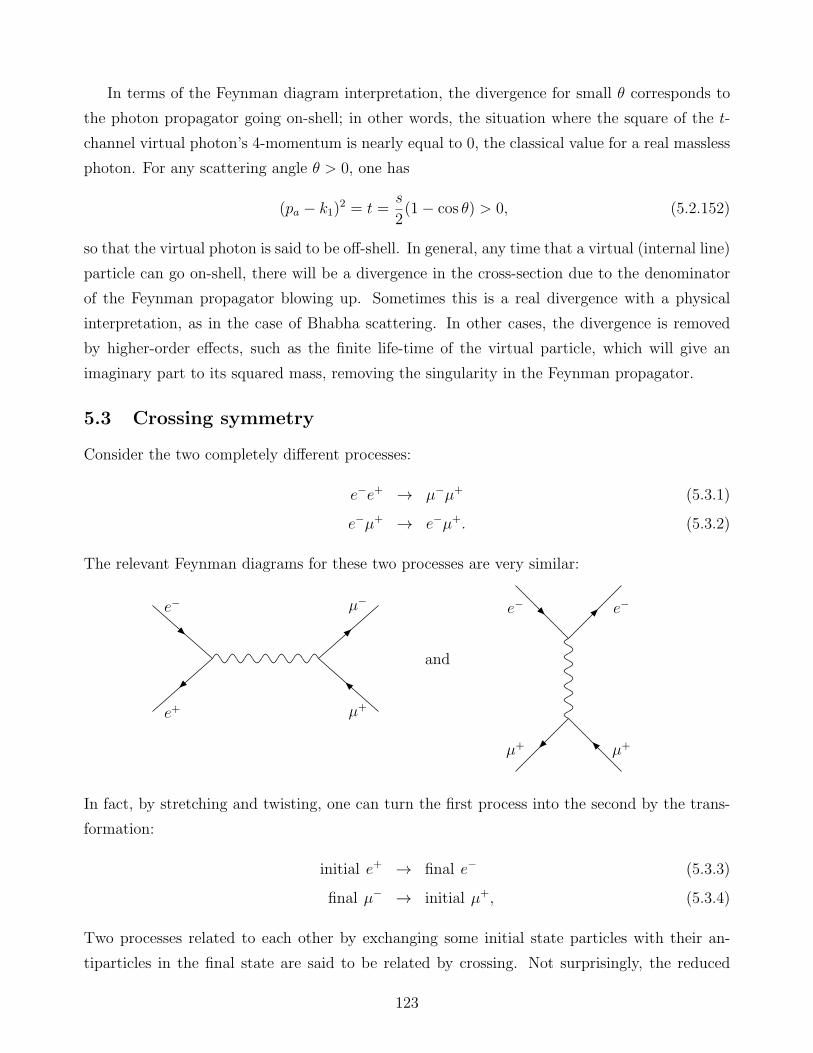
In terms of the Feynman diagram interpretation, the divergence for small θ corresponds to

the photon propagator going on-shell; in other words, the situation where the square of the t-

channel virtual photon’s 4-momentum is nearly equal to 0, the classical value for a real massless

photon. For any scattering angle θ > 0, one has

(pa − k1)2 = t =s

2(1− cos θ) > 0, (5.2.152)

so that the virtual photon is said to be off-shell. In general, any time that a virtual (internal line)

particle can go on-shell, there will be a divergence in the cross-section due to the denominator

of the Feynman propagator blowing up. Sometimes this is a real divergence with a physical

interpretation, as in the case of Bhabha scattering. In other cases, the divergence is removed

by higher-order effects, such as the finite life-time of the virtual particle, which will give an

imaginary part to its squared mass, removing the singularity in the Feynman propagator.

5.3 Crossing symmetry

Consider the two completely different processes:

e−e+ → µ−µ+ (5.3.1)

e−µ+ → e−µ+. (5.3.2)

The relevant Feynman diagrams for these two processes are very similar:

e− µ−

e+ µ+

and

µ+

e−

µ+

e−

In fact, by stretching and twisting, one can turn the first process into the second by the trans-

formation:

initial e+ → final e− (5.3.3)

final µ− → initial µ+, (5.3.4)

Two processes related to each other by exchanging some initial state particles with their an-

tiparticles in the final state are said to be related by crossing. Not surprisingly, the reduced

123

matrix elements for these processes are also quite similar. For example, in the high-energy limit√s≫ mµ,

1

4

∑

spins

|Me−e+→µ−µ+ |2 = 2e4(u2 + t2

s2

), (5.3.5)

1

4

∑

spins

|Me−µ+→e−µ+ |2 = 2e4(u2 + s2

t2

). (5.3.6)

This similarity is generalized and made more precise by the following theorem.

Crossing Symmetry Theorem: Suppose two Feynman diagrams with reduced

matrix elementsM andM′ are related by the exchange (“crossing”) of some initial

state particles and antiparticles for the corresponding final state antiparticles and

particles. If the crossed particles have 4-momenta P µ1 , . . . P

µn inM, then

∑spins |M|2

can be obtained by substituting P ′µi = −P µ

i into the mathematical expression for∑

spins |M′|2, as follows:∑

spins

|M(P µ1 , . . . , P

µn , . . .)|2 = (−1)F

∑

spins

|M′(P ′µ1 , . . . , P

′µn , . . .)|2

∣∣∣∣∣P ′µi

→−Pµi

, (5.3.7)

with the other (uncrossed) particle 4-momenta unaffected. Here F is the number of

fermion lines that were crossed.

If pµ = (E, ~p ) is a valid physical 4-momentum, then p′µ = (−E,−~p ) is never a physical 4-

momentum, since it has negative energy. So the relation between the two diagrams is a formal

one rather than a relation between physical reduced matrix elements that would actually be

measured; when one of the matrix elements involves the 4-momenta appropriate for a physical

process, the other one does not. However, it is still perfectly valid as a mathematical relation,

and therefore extremely useful. In general, if one has calculated the cross-section or reduced

matrix element for one process, one can obtain the results for several “crossed” processes by

merely substituting momenta, with no additional labor. Equation (5.3.7) might look dubious

at first, since it may look like the right-hand side is negative for odd F . However, the point is

that when the expression for |M′|2 is analytically continued to unphysical momenta, it always

flips sign for odd F . We will see this in some examples later.

5.3.1 e−µ+ → e−µ+ and e−µ− → e−µ−

Let us apply crossing symmetry to the example of eqs. (5.3.1) and (5.3.2) by assigning primed

momenta to the Feynman diagram for e−e+ → µ−µ+:

initial state

e− ↔ p′ae+ ↔ p′b

(5.3.8)

124

final state

µ− ↔ k′1µ+ ↔ k′2.

(5.3.9)

Label the momenta in the crossed Feynman diagram (for e−µ+ → e−µ+) without primes:

initial state

e− ↔ paµ+ ↔ pb

(5.3.10)

final state

e− ↔ k1µ+ ↔ k2.

(5.3.11)

Then the Crossing Symmetry Theorem tells us that we can get the reduced matrix element

for the process e−µ+ → e−µ+ as a function of physical momenta pa, pb, k1, k2 by substituting

unphysical momenta

p′a = pa; p′b = −k1; k′1 = −pb; k′2 = k2, (5.3.12)

into the formula for the reduced matrix element for the process e−e+ → µ−µ+. This means that

we can identify:

s′ = (p′a + p′b)2 = (pa − k1)2 = t, (5.3.13)

t′ = (p′a − k′1)2 = (pa + pb)2 = s, (5.3.14)

u′ = (p′a − k′2)2 = (pa − k2)2 = u. (5.3.15)

In other words, crossing symmetry tells us that the formulas for the reduced matrix elements for

these two processes are just related by the exchange of s and t, as illustrated in the high-energy

limit in eqs. (5.3.5) and (5.3.6). Since we had already derived the result for the first process in

section 5.2.1, the second result has been obtained for free. Note that we could have obtained

the particular result (5.3.6) even more easily just by noting that the calculation for the reduced

matrix element of e−µ+ → e−µ+ is exactly the same as for Bhabha scattering, except that only

the t-channel diagram exists in the former case. So one only keeps the contribution with t (not

s or u) in the denominator, since that corresponds to the t-channel diagram.

We can carry this further by considering another process also related by crossing to the two

just studied:

e−µ− → e−µ−, (5.3.16)

with physical momenta:

initial state

e− ↔ paµ− ↔ pb

(5.3.17)

final state

e− ↔ k1µ− ↔ k2

. (5.3.18)

125

This time, the Crossing Symmetry Theorem tells us that we can identify the matrix element by

again starting with the reduced matrix element for e−e+ → µ−µ+ and replacing:

p′a = pa; p′b = −k1; k′1 = k2; k′2 = −pb, (5.3.19)

so that

s′ = (p′a + p′b)2 = (pa − k1)2 = t, (5.3.20)

t′ = (p′a − k′1)2 = (pa − k2)2 = u, (5.3.21)

u′ = (p′a − k′2)2 = (pa + pb)2 = s. (5.3.22)

Here the primed Mandelstam variable are the unphysical ones for the e−e+ → µ−µ+ process,

and the unprimed ones are for the desired process e−µ− → e−µ−. We can therefore infer, from

eq. (5.3.5), that

1

4

∑

spins

|Me−µ−→e−µ− |2 = 2e4(s2 + u2

t2

), (5.3.23)

by doing the substitutions indicated by eqs. (5.3.20)-(5.3.22).

By comparing eq. (5.3.6) to eq. (5.3.23), one sees that the spin averaged and summed squared

matrix elements for the two processes are actually the same; the charge of the muon does not

matter at leading order. Because we are neglecting the muon mass, the kinematics relating t

and u to the scattering angle θ between the initial-state electron and the final state electron in

these two cases is just the same as in Bhabha scattering:

t = −s2(1− cos θ); u = −s

2(1 + cos θ). (5.3.24)

Therefore, putting eq. (5.3.23) into eq. (4.5.49) with |~pa| = |~k1| and using e2 = 4πα, we obtain

the differential cross-section for e−µ± → e−µ±:

dσ

d(cos θ)=

πα2

s

(u2 + s2

t2

)(5.3.25)

=πα2

2s

5 + 2 cos θ + cos2 θ

(1− cos θ)2. (5.3.26)

Note that this again diverges for forward scattering cos θ → 1.

5.3.2 Møller scattering (e−e− → e−e−)

As another example, let us consider the case of Møller scattering:

e−e− → e−e−. (5.3.27)

There are two Feynman diagrams for this process:

126

e−, k2

e−, k1

e−, pb

e−, pa

and

e−, k2

e−, k1

e−, pb

e−, pa

Now, nobody can stop us from getting the result for this process by applying the Feynman

rules to get the reduced matrix element, taking the complex square, summing and averaging

over spins, and computing the Dirac traces. However, an easier way is to note that this is a

crossed version of Bhabha scattering, which we studied earlier. Making a table of the momenta:

Bhabha Møller (5.3.28)

e− ↔ p′a e− ↔ pa (5.3.29)

e+ ↔ p′b e− ↔ pb (5.3.30)

e− ↔ k′1 e− ↔ k1 (5.3.31)

e+ ↔ k′2 e− ↔ k2, (5.3.32)

we see that crossing symmetry allows us to compute the Møller scattering by identifying the

(initial state positron, final state positron) in Bhabha scattering with the (final state electron,

initial state electron) in Møller scattering, so that:

p′a = pa p′b = −k2 k′1 = k1 k′2 = −pb. (5.3.33)

Therefore, the Møller scattering reduced matrix element is obtained by putting

s′ = (p′a + p′b)2 = (pa − k2)2 = u (5.3.34)

t′ = (p′a − k′1)2 = (pa − k1)2 = t (5.3.35)

u′ = (p′a − k′2)2 = (pa + pb)2 = s (5.3.36)

into the corresponding result for Bhabha scattering. Using the results of eq. (5.2.144)-(5.2.146),

we get:

1

4

∑

spins

|Me−e−→e−e− |2 = 2e2(s2 + t2

u2+s2 + u2

t2+

2s2

ut

). (5.3.37)

127

Again, if we keep only the t-channel part (that is, the part with t2 in the denominator), we

recover the result for e−µ± → e−µ± in the previous section.

Applying eq. (4.5.49), we find the differential cross-section:

dσe−e−→e−e−

d(cos θ)=

1

32πs

1

4

∑

spins

|Me−e−→e−e− |2 (5.3.38)

=πα2

s

(s2 + t2

u2+s2 + u2

t2+

2s2

ut

)(5.3.39)

=2πα2

s

(3 + cos2 θ

1− cos2 θ

)2

. (5.3.40)

Just as in the cases in the previous sections, t = −s(1− cos θ)/2 and u = −2(1+ cos θ)/2 where

θ is the angle between the initial-state and final-state electrons. However, in this case there

is a special feature, because the two electrons in the final state are indistinguishable particles.

This means that the final state with an electron coming out at angles (θ, φ) is actually the same

quantum state as the one with an electron coming out at angles (π − θ, −φ). (As a check,

note that eq. (5.3.40) is invariant under cos θ → − cos θ. We have already integrated over the

angle φ.) Therefore, to avoid overcounting we must only integrate over half the range of θ, or

equivalently divide the total cross-section by 2. So, we have a tricky and crucial factor of 1/2

in the total cross-section:

σe−e−→e−e− =1

2

∫ cos θcut

− cos θcut

dσe−e−→e−e−

d(cos θ)d(cos θ). (5.3.41)

To obtain a finite value for the total cross-section, we had to also impose a cut on the minimum

scattering angle θcut that we require in order to say that a scattering event should be counted.

5.4 Gauge invariance in Feynman diagrams

Let us now turn to the issue of gauge invariance as it is manifested in QED Feynman diagrams.

Recall that when we found the Feynman propagator for a photon, it contained a term that

depended on an arbitrary parameter ξ. We have been working with ξ = 1 (Feynman gauge).

Consider what the matrix element for the process e−e+ → µ−µ+ would be if instead we let ξ

remain unfixed. Instead of eq. (5.2.2), we would have

M = (vbγµua)(u1γ

νv2)ie2

(pa + pb)2

[−gµν + (1− ξ)(pa + pb)µ(pa + pb)ν

(pa + pb)2

]. (5.4.1)

If the answer is to be independent of ξ, then it must be true that the new term proportional to

(1− ξ) gives no contribution. This can be easily proved by observing that it contains the factor

(vbγµua)(pa + pb)µ = vb/paua + vb/pbua = mvbua −mvbua = 0. (5.4.2)

128

Here we have applied the Dirac equation, as embodied in eqs. (A.2.24) and (A.2.25), to write

/paua = mua and vb/pb = −m/pb. For any photon propagator connected (at either end) to an

external fermion line, the proof is similar. And, in general, one can show that the 1 − ξ term

will always cancel when one includes all Feynman diagrams contributing to a particular process.

So we can choose the most convenient value of ξ, which is usually ξ = 1.

Another aspect of gauge invariance involves a feature that we have not explored in an example

so far: external state photons. Recall that the Feynman rules associate factors of ǫµ(p, λ) and

ǫ∗µ(p, λ) to initial or final state photons, respectively. Now, making a gauge transformation on

the photon field results in:

Aµ → Aµ + ∂µΛ (5.4.3)

where Λ is any function. In momentum space, the derivative ∂µ is proportional to pµ. So, in

terms of the polarization vector for the electromagnetic field, a gauge transformation is

ǫµ(p, λ)→ ǫµ(p, λ) + apµ (5.4.4)

where a is any quantity. The polarization vector and momentum for a physical photon satisfy

ǫ2 = −1 and ǫ · p = 0 and p2 = 0. As a consistency check, note that if these relations are

satisfied, then they will also be obeyed after the gauge transformation (5.4.4).

Gauge invariance implies that the reduced matrix element should also be unchanged after

the substitution in eq. (5.4.4). The reduced matrix element for a process with an external state

photon with momentum pµ and polarization label λ can always be written in the form:

M =Mµǫµ(p, λ), (5.4.5)

which defines Mµ. Since M must be invariant under a gauge transformation, it follows from

eq. (5.4.4) that

Mµpµ = 0. (5.4.6)

This relation is known as the Ward identity for QED. It says that if we replace the polarization

vector for any photon by the momentum of that photon, then the reduced matrix element should

become 0. This is a nice consistency check on calculations.

Another nice consequence of the Ward identity is that it provides for a simplified way to

sum or average over unmeasured photon polarization states. Consider a photon with momentum

taken to be along the positive z axis, with pµ = (P, 0, 0, P ). Summing over the two polarization

vectors in eqs. (5.1.26)-(5.1.27), we have:

2∑

λ=1

|M|2 =2∑

λ=1

MµM∗νǫ

µ(p, λ)ǫ∗ν(p, λ) = |M1|2 + |M2|2, (5.4.7)

129

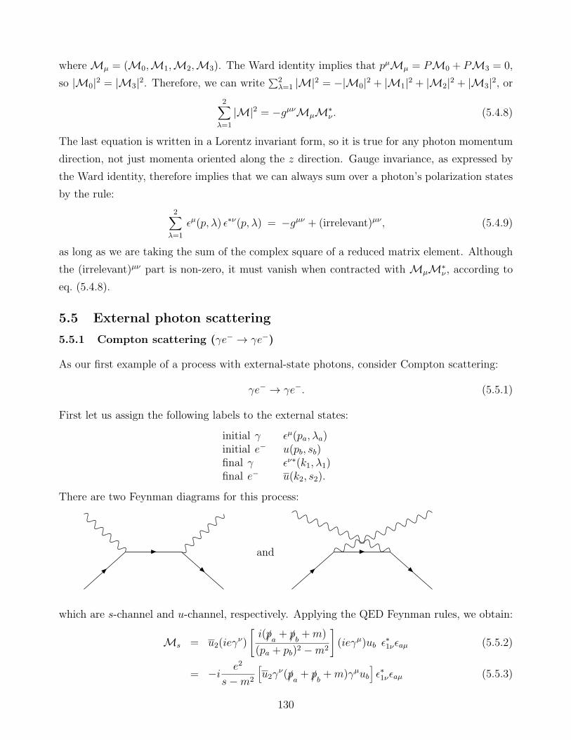
whereMµ = (M0,M1,M2,M3). The Ward identity implies that pµMµ = PM0 + PM3 = 0,

so |M0|2 = |M3|2. Therefore, we can write∑2

λ=1 |M|2 = −|M0|2 + |M1|2 + |M2|2 + |M3|2, or2∑

λ=1

|M|2 = −gµνMµM∗ν . (5.4.8)

The last equation is written in a Lorentz invariant form, so it is true for any photon momentum

direction, not just momenta oriented along the z direction. Gauge invariance, as expressed by

the Ward identity, therefore implies that we can always sum over a photon’s polarization states

by the rule:

2∑

λ=1

ǫµ(p, λ) ǫ∗ν(p, λ) = −gµν + (irrelevant)µν , (5.4.9)

as long as we are taking the sum of the complex square of a reduced matrix element. Although

the (irrelevant)µν part is non-zero, it must vanish when contracted withMµM∗ν , according to

eq. (5.4.8).

5.5 External photon scattering

5.5.1 Compton scattering (γe− → γe−)

As our first example of a process with external-state photons, consider Compton scattering:

γe− → γe−. (5.5.1)

First let us assign the following labels to the external states:

initial γ ǫµ(pa, λa)initial e− u(pb, sb)final γ ǫν∗(k1, λ1)final e− u(k2, s2).

There are two Feynman diagrams for this process:

and

which are s-channel and u-channel, respectively. Applying the QED Feynman rules, we obtain:

Ms = u2(ieγν)

[i(/pa + /pb +m)

(pa + pb)2 −m2

](ieγµ)ub ǫ

∗1νǫaµ (5.5.2)

= −i e2

s−m2

[u2γ

ν(/pa + /pb +m)γµub]ǫ∗1νǫaµ (5.5.3)

130

and

Mu = u2(ieγµ)

[i(/pb − /k1 +m)

(pb − k1)2 −m2

](ieγν)ub ǫ

∗1νǫaµ (5.5.4)

= −i e2

u−m2

[u2γ

µ(/pb − /k1 +m)γνub]ǫ∗1νǫaµ. (5.5.5)

Before squaring the total reduced matrix element, it is useful to simplify. So we note that:

(/pb +m)γµub = /pb, γµub − γµ(/pb −m)ub (5.5.6)

= pbσγσ, γµub + 0 (5.5.7)

= 2pbσgσµub (5.5.8)

= 2pµbub, (5.5.9)

where we have used eq. (A.2.24). So the reduced matrix element is:

M = −ie2ǫ∗1νǫaµ u2

[1

s−m2

(γν/paγ

µ + 2pµb γν)+

1

u−m2(−γµ/k1γν + 2pνbγ

µ)]ub. (5.5.10)

Taking the complex conjugate of eq. (5.5.10) gives:

M∗ = ie2ǫ1σǫ∗aρ ub

[1

s−m2(γρ/paγ

σ + 2pρbγσ) +

1

u−m2(−γσ/k1γρ + 2pσb γ

ρ)]u2. (5.5.11)

Now we multiply together eqs. (5.5.10) and (5.5.11), and average over the initial photon polar-

ization λa and sum over the final photon polarization λ1, using

1

2

2∑

λa=1

ǫaµǫ∗aρ = −

1

2gµρ + irrelevant, (5.5.12)

2∑

λ1=1

ǫ∗1νǫ1σ = −gνσ + irrelevant, (5.5.13)

to obtain:

1

2

∑

λa,λ1

|M|2 = e4

2

u2

[1

s−m2(γν/paγ

µ + 2pµb γν) +

1

u−m2(−γµ/k1γν + 2pνbγ

µ)]ub

ub

[1

s−m2(γµ/paγν + 2pbµγν) +

1

u−m2(−γν/k1γµ + 2pbνγµ)

]u2

. (5.5.14)

Next we can average over sb, and sum over s2, using the usual tricks:

1

2

∑

sb

ubub =1

2(/pb +m), (5.5.15)

∑

s2

u2 . . . u2 = Tr[. . . (/k2 +m)]. (5.5.16)

131

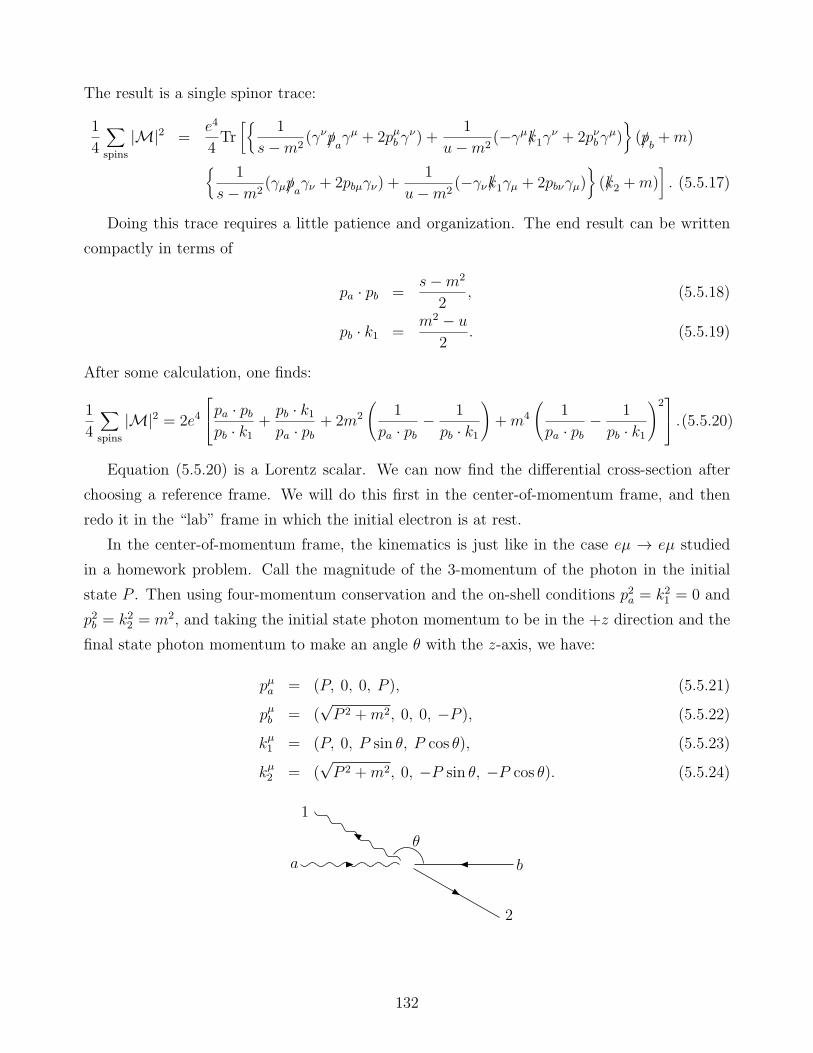
The result is a single spinor trace:

1

4

∑

spins

|M|2 =e4

4Tr[

1

s−m2(γν/paγ

µ + 2pµb γν) +

1

u−m2(−γµ/k1γν + 2pνbγ

µ)(/pb +m)

1

s−m2(γµ/paγν + 2pbµγν) +

1

u−m2(−γν/k1γµ + 2pbνγµ)

(/k2 +m)

]. (5.5.17)

Doing this trace requires a little patience and organization. The end result can be written

compactly in terms of

pa · pb =s−m2

2, (5.5.18)

pb · k1 =m2 − u

2. (5.5.19)

After some calculation, one finds:

1

4

∑

spins

|M|2 = 2e4

pa · pbpb · k1

+pb · k1pa · pb

+ 2m2

(1

pa · pb− 1

pb · k1

)+m4

(1

pa · pb− 1

pb · k1

)2 .(5.5.20)

Equation (5.5.20) is a Lorentz scalar. We can now find the differential cross-section after

choosing a reference frame. We will do this first in the center-of-momentum frame, and then

redo it in the “lab” frame in which the initial electron is at rest.

In the center-of-momentum frame, the kinematics is just like in the case eµ → eµ studied

in a homework problem. Call the magnitude of the 3-momentum of the photon in the initial

state P . Then using four-momentum conservation and the on-shell conditions p2a = k21 = 0 and

p2b = k22 = m2, and taking the initial state photon momentum to be in the +z direction and the

final state photon momentum to make an angle θ with the z-axis, we have:

pµa = (P, 0, 0, P ), (5.5.21)

pµb = (√P 2 +m2, 0, 0, −P ), (5.5.22)

kµ1 = (P, 0, P sin θ, P cos θ), (5.5.23)

kµ2 = (√P 2 +m2, 0, −P sin θ, −P cos θ). (5.5.24)

a b

2

1

θ

132

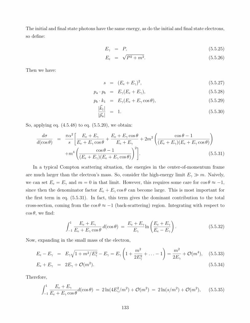
The initial and final state photons have the same energy, as do the initial and final state electrons,

so define:

Eγ = P, (5.5.25)

Ee =√P 2 +m2. (5.5.26)

Then we have:

s = (Ee + Eγ)2, (5.5.27)

pa · pb = Eγ(Ee + Eγ), (5.5.28)

pb · k1 = Eγ(Ee + Eγ cos θ), (5.5.29)

|~k1||~pa|

= 1. (5.5.30)

So, applying eq. (4.5.48) to eq. (5.5.20), we obtain:

dσ

d(cos θ)=

πα2

s

[Ee + Eγ

Ee + Eγ cos θ+Ee + Eγ cos θ

Ee + Eγ

+ 2m2

(cos θ − 1

(Ee + Eγ)(Ee + Eγ cos θ)

)

+m4

(cos θ − 1

(Ee + Eγ)(Ee + Eγ cos θ)

)2]. (5.5.31)

In a typical Compton scattering situation, the energies in the center-of-momentum frame

are much larger than the electron’s mass. So, consider the high-energy limit Eγ ≫ m. Naively,

we can set Ee = Eγ and m = 0 in that limit. However, this requires some care for cos θ ≈ −1,since then the denominator factor Ee + Eγ cos θ can become large. This is most important for

the first term in eq. (5.5.31). In fact, this term gives the dominant contribution to the total

cross-section, coming from the cos θ ≈ −1 (back-scattering) region. Integrating with respect to

cos θ, we find:

∫ 1

−1

Ee + Eγ

Ee + Eγ cos θd(cos θ) =

Ee + Eγ

Eγ

ln

(Ee + Eγ

Ee − Eγ

). (5.5.32)

Now, expanding in the small mass of the electron,

Ee − Eγ = Eγ

√1 +m2/E2

γ − Eγ = Eγ

(1 +

m2

2E2γ

+ . . .− 1

)=

m2

2Eγ

+O(m4), (5.5.33)

Ee + Eγ = 2Eγ +O(m2). (5.5.34)

Therefore,

∫ 1

−1

Ee + Eγ

Ee + Eγ cos θd(cos θ) = 2 ln(4E2

γ/m2) +O(m2) = 2 ln(s/m2) +O(m2), (5.5.35)

133

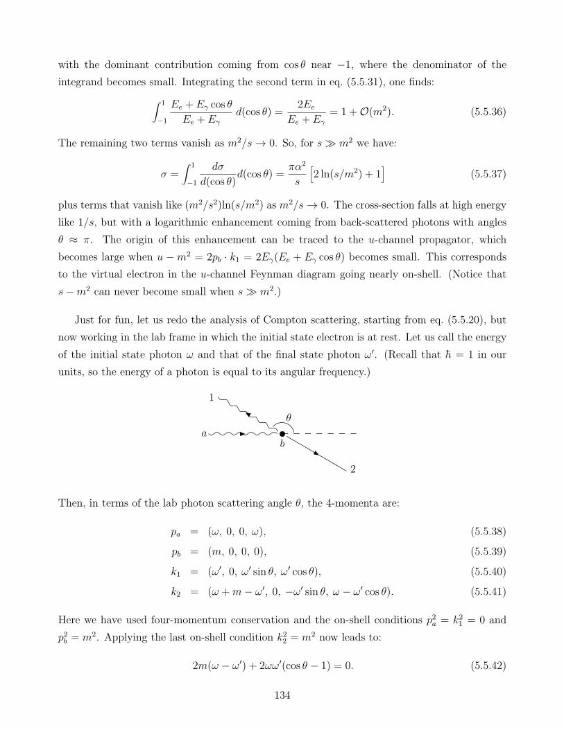
with the dominant contribution coming from cos θ near −1, where the denominator of the

integrand becomes small. Integrating the second term in eq. (5.5.31), one finds:

∫ 1

−1

Ee + Eγ cos θ

Ee + Eγ

d(cos θ) =2Ee

Ee + Eγ

= 1 +O(m2). (5.5.36)

The remaining two terms vanish as m2/s→ 0. So, for s≫ m2 we have:

σ =∫ 1

−1

dσ

d(cos θ)d(cos θ) =

πα2

s

[2 ln(s/m2) + 1

](5.5.37)

plus terms that vanish like (m2/s2)ln(s/m2) as m2/s→ 0. The cross-section falls at high energy

like 1/s, but with a logarithmic enhancement coming from back-scattered photons with angles

θ ≈ π. The origin of this enhancement can be traced to the u-channel propagator, which

becomes large when u −m2 = 2pb · k1 = 2Eγ(Ee + Eγ cos θ) becomes small. This corresponds

to the virtual electron in the u-channel Feynman diagram going nearly on-shell. (Notice that

s−m2 can never become small when s≫ m2.)

Just for fun, let us redo the analysis of Compton scattering, starting from eq. (5.5.20), but

now working in the lab frame in which the initial state electron is at rest. Let us call the energy

of the initial state photon ω and that of the final state photon ω′. (Recall that h = 1 in our

units, so the energy of a photon is equal to its angular frequency.)

ab

2

1

θ

Then, in terms of the lab photon scattering angle θ, the 4-momenta are:

pa = (ω, 0, 0, ω), (5.5.38)

pb = (m, 0, 0, 0), (5.5.39)

k1 = (ω′, 0, ω′ sin θ, ω′ cos θ), (5.5.40)

k2 = (ω +m− ω′, 0, −ω′ sin θ, ω − ω′ cos θ). (5.5.41)

Here we have used four-momentum conservation and the on-shell conditions p2a = k21 = 0 and

p2b = m2. Applying the last on-shell condition k22 = m2 now leads to:

2m(ω − ω′) + 2ωω′(cos θ − 1) = 0. (5.5.42)

134

This can be used to solve for ω′ in terms of cos θ, or vice versa:

ω′ =ω

1 + ωm(1− cos θ)

; (5.5.43)

cos θ = 1− m(ω − ω′)

ωω′ . (5.5.44)

In terms of lab-frame variables, one has:

pa · pb = ωm; (5.5.45)

pb · k1 = ω′m, (5.5.46)

so that, from eq. (5.5.20):

1

4

∑

spins

|M|2 = 2e4[ω

ω′ +ω′

ω+ 2m

(1

ω− 1

ω′

)+m2

(1

ω− 1

ω′

)2]. (5.5.47)

This can be simplified slightly by using

m(1

ω− 1

ω′

)= cos θ − 1, (5.5.48)

which follows from eq. (5.5.42), so that

1

4

∑

spins

|M|2 = 2e4[ω

ω′ +ω′

ω− sin2 θ

]. (5.5.49)

Now to find the differential cross-section, we must apply eq. (4.5.32):

dσ =1

4EaEb|~va − ~vb|

(1

4|M|2

)dΦ2, (5.5.50)

where dΦ2 is the two-body Lorentz-invariant phase space, as defined in eq. (4.5.33), for the final

state particles in the lab frame. Evaluating the prefactors for the case at hand:

Ea = ω, (5.5.51)

Eb = m, (5.5.52)

|~va − ~vb| = 1− 0 = 1. (5.5.53)

(Recall that the speed of the photon is c = 1.)

The two-body phase space in the lab frame is:

dΦ2 = (2π)4 δ(4)(k1 + k2 − pa − pb)d3~k1

(2π)32E1

d3~k2(2π)32E2

(5.5.54)

= δ(3)(~k1 + ~k2 − ωz) δ(ω′ + E2 − ω −m)d3~k1

16π2ω′E2

d3~k2, (5.5.55)

135

where ω′ is now defined to be equal to E1 = |~k1| and E2 is defined to be√|~k2|2 +m2. Performing

the ~k2 integral using the 3-momentum delta function just sets ~k2 = ωz − ~k1, resulting in:

dΦ2 = δ(ω′ + E2 − ω −m)d3~k1

16π2ω′E2

, (5.5.56)

where now

E2 =√ω′2 − 2ωω′ cos θ + ω2 +m2. (5.5.57)

The phase space for the final state photon can be simplified by writing it in terms of angular

coordinates and doing the integral∫dφ = 2π:

d3~k1 = dφ d(cos θ) ω′2 dω′ = 2π d(cos θ) ω′2 dω′. (5.5.58)

Therefore,

dΦ2 = δ(ω′ + E2 − ω −m)d(cos θ)ω′dω′

8πE2

. (5.5.59)

In order to do the ω′ integral, it is simplest, as usual, to make a change of integration variables

to the argument of the delta function. So, defining

K = ω′ + E2 − ω −m, (5.5.60)

we have

dK

dω′ = 1 +ω′ − ω cos θ

E2

. (5.5.61)

Therefore,

ω′dω′

E2

=ω′dK

E2 + ω′ − ω cos θ. (5.5.62)

Performing the dK integration sets K = 0, so E2 = ω+m−ω′. Using eq. (5.5.62) in eq. (5.5.59)

gives

dΦ2 =ω′

m+ ω(1− cos θ)

d(cos θ)

8π=

ω′2

8πmωd(cos θ), (5.5.63)

where eq. (5.5.43) has been used to simplify the denominator. Finally using this in eq. (5.5.50)

yields:

dσ =

1

4

∑

spins

|M|2 ω′2

32πmω2d(cos θ), (5.5.64)

136

so that, putting in eq. (5.5.49),

dσ

d(cos θ)=πα2

m2

(ω′

ω

)2 [ω′

ω+ω

ω′ − sin2 θ

]. (5.5.65)

This result is the Klein-Nishina formula.

As in the center-of-momentum frame, the largest differential cross-section is found for back-

scattered photons with cos θ = −1, which corresponds to the smallest possible final-state photon

energy ω′. Notice that, according to eq. (5.5.43), when ω ≫ m, one gets very low energies ω′

when the photon is back-scattered. One can now integrate the lab-frame differential cross-

section∫ 1−1 d(cos θ) to get the total cross-section, using the dependence of ω′ on cos θ as given

in eq. (5.5.43). The result is:

σ = πα2

[(1

ωm− 2

ω2− 2m

ω3

)ln(1 +

2ω

m

)+

4

ω2+

2(m+ ω)

m(m+ 2ω)2

]. (5.5.66)

In the high-energy (small m) limit, this becomes:

σ = πα2[

1

ωmln(2ω

m

)+

1

2ωm+ . . .

]. (5.5.67)

We can re-express this in terms of the Mandelstam variable s = (ω +m)2 − ω2 = 2ωm+m2 ≈2ωm,

σ =πα2

s

[2ln(s/m2) + 1 + . . .

]. (5.5.68)

Equation (5.5.68) is the same result that we found in the center-of-momentum frame, eq. (5.5.37).

This is an example of a general fact: the total cross-section does not depend on the choice of

reference frame, provided that one boosts along a direction parallel to the collision axis. To

see why, one need only look at the definition of the total cross-section given in eq. (4.5.2). The

numbers of particles NS, Na, and Nb can be simply counted, and so certainly do not depend on

any choice of inertial reference frame, while the area A is invariant under Lorentz boosts along

the collision axis.

The low-energy Thomson scattering limit is also interesting. In the lab frame, ω ≪ m implies

ω′/ω = 1, so that

dσ

d(cos θ)=πα2

m2(1 + cos2 θ), (5.5.69)

which is independent of energy. The total cross-section in this limit is then

σ =8πα2

3m2. (5.5.70)

Unlike the case of high-energy Compton scattering, Thomson scattering is symmetric under

θ → π − θ, with a factor of 2 enhancement in the forward (θ = 0) and backward (θ = π)

directions compared to right-angle (θ = π/2) scattering.

137

5.5.2 e+e− → γγ

As our final example of a QED process let us consider e+e− → γγ in the high-energy limit. We

could always compute the reduced matrix element starting from the Feynman rules. However,

since we have already done Compton scattering, it is easier to use crossing. Labeling the physical

momenta for Compton scattering now with primes, we can make the following comparison table:

Compton e+e− → γγ (5.5.71)

γ ↔ p′a e+ ↔ pa (5.5.72)

e− ↔ p′b e− ↔ pb (5.5.73)

γ ↔ k′1 γ ↔ k1 (5.5.74)

e− ↔ k′2 γ ↔ k2. (5.5.75)

For convenience, we have chosen e+ to be labeled by “a”, so that the initial-state e− can have

the same label “b” in both processes. Then according to the Crossing Symmetry Theorem, we

can obtain∑

spins |Me+e−→γγ|2 by making the replacements

p′a = −k2; p′b = pb; k′1 = k1; k′2 = −pa (5.5.76)

in the Compton scattering result (for small m):

∑

spins

|Mγe−→γe− |2 = 8e4(p′a · p′bp′b · k′1

+p′b · k′1p′a · p′b

), (5.5.77)

obtained from eq. (5.5.20). Because the crossing involves one fermion (a final state electron

changes into an initial state positron), there is also a factor of (−1)1 = −1, according to

eq. (5.3.7). So, the result is:

∑

spins

|Me+e−→γγ|2 = (−1)8e4(−k2 · pbpb · k1

+pb · k1−k2 · pb

)(5.5.78)

= 8e4(k2 · pbpb · k1

+pb · k1k2 · pb

). (5.5.79)

The situation here is 2 → 2 massless particle scattering, so we can steal the kinematics

information directly from eqs. (5.2.139)-(5.2.143). The relevant facts for the present case are:

pb · k1 = −u2=s

4(1 + cos θ), (5.5.80)

pb · k2 = − t2=s

4(1− cos θ). (5.5.81)

Therefore,

1

4

∑

spins

|Me+e−→γγ|2 = 2e4(t

u+u

t

)= 4e4

(1 + cos2 θ

sin2 θ

). (5.5.82)

138

It is a useful check, and a vindication of the (−1)F factor in the Crossing Symmetry Theorem,

that this is positive! Now plugging this into the formula eq. (4.5.49) for the differential cross-

section, we get:

dσ

d cos(θ)=

2πα2

s

(1 + cos2 θ

sin2 θ

). (5.5.83)

This cross-section is symmetric as θ → π − θ. That was inevitable, since the two final state

photons are identical; the final state in which a photon is observed coming out at a (θ, φ) is

actually the same as a state in which a photon is observed at an angle (π − θ,−φ). When we

find the total cross-section, we should therefore divide by 2 (or just integrate over half of the

range for cos θ) to avoid overcounting. This is the same overcounting issue for identical final

state particles that arose for Møller scattering at the end of section 5.3.2.

The integrand in eq. (5.5.83) diverges for sin θ = 0. This is because we have set m = 0 in

the kinematics, which is not valid for scattering very close to the collision axis. If you put back

non-zero m, you will find that instead of diverging, the total cross-section features a logarithmic

enhancement ln(s/m2) coming from small sin θ. In a real e−e+ → γγ experiment, however,

photons very close to the electron and positron beams will not be seen by any detector. The

observable cross-section in one of these colliding beam experiments is something more like

σcut =1

2

∫ cos θcut

− cos θcut

dσ

d(cos θ)d(cos θ) (5.5.84)

=2πα2

s

[ln

(1 + cos θcut1− cos θcut

)− cos θcut

]. (5.5.85)

(You can easily check that this is a positive and increasing function of cos θcut.) On the other

hand, if you are interested in the total cross-section for electron-positron annihilation with no

cuts applied on the angle, then you must take into account the non-zero electron mass. Redoing

everything with m≪ √s but non-zero, you can show:

σ =2πα2

s

[ln(

s

2m2

)− 1

]. (5.5.86)

The logarithmic enhancement at large s in this formula comes entirely from the sin θ ≈ 0 region.

Note that this formula is just what you would have gotten by plugging in

cos θcut = 1− 4m2/s (5.5.87)

into eq. (5.5.85), for smallm. In this sense, the finite mass of the electron “cuts off” the would-be

logarithmic divergence of the cross-section for small sin θ.

139

6 Decay Processes

6.1 Decay rates and partial widths

So far, we have studied only 2→ 2 scattering processes. This is because in QED as a stand-alone

theory, the fundamental particles are stable. Photons cannot decay into anything else (in any

theory), because they are massless. The electron is the lightest particle that carries charge, so

it cannot decay because of charge conservation. The photon interaction vertex with a fermion

line does not change the type of fermion. So if there is only a muon in the initial state, you

can easily convince yourself that there must be at least one muon in the final state. Going to

the rest frame of the initial muon, the total energy of the process is simply mµ, but the energy

of the final state would have to be larger than this, so if only QED interactions are allowed,

the muon must also be stable. The weak interactions get around this by allowing interaction

vertices that change the fermion type. Moreover, bound states can decay even in QED.

For any type of unstable particle, the probability that a decay will occur in a very short

interval of time ∆t should be proportional to ∆t. So we can define the decay rate Γ [also

known as the decay width; it is equal to the resonance width in eq. (1.2.1)] as the constant of

proportionality:

(Probability of decay in time ∆t) = Γ∆t. (6.1.1)

Suppose we observe the decays of a large sample of particles of this type, all at rest. If the

number of particle at time t is denoted N(t), then the number of particles remaining a short

time later is therefore:

N(t+∆t) = (1− Γ∆t)N(t). (6.1.2)

It follows that

dN

dt= lim

∆t→0

N(t+∆t)−N(t)

∆t= −ΓN, (6.1.3)

so that

N(t) = e−ΓtN(0). (6.1.4)

When one has computed or measured Γ for some particle, it is traditional and sensible to quote

the result as measured in the rest frame of the particle. If the particle is moving with velocity

β, then because of relativistic time dilation, the survival probability for a particular particle as

a function of the laboratory time t is:

(Probability of particle survival) = e−Γt√

1−β2

. (6.1.5)

140

The quantity

τ = 1/Γ (6.1.6)

is also known as the mean lifetime of the particle at rest. [Putting in the units recovers eq. (1.2.2);

see eq. (A.1.6).] There is often more than one final state available for a decaying particle. One

can then compute or measure the decay rates into particular final states. The rate Γ for a

particular final state or class of final states is called a partial width. The sum of all exclusive

partial widths should add up to the total decay rate, of course.

Consider a process in which a particle at rest with 4-momentum

pµ = (M, 0, 0, 0) (6.1.7)

decays to several particles with 4-momenta ki and masses mi. Given the reduced matrix element

M for this process, one can show by arguments similar to those in 4.5 for cross-sections that

the differential decay rate is:

dΓ =1

2M|M|2 dΦn, (6.1.8)

where

dΦn = (2π)4δ(4)(p−∑

i

ki)n∏

i=1

d3~ki(2π)32Ei

(6.1.9)

is the n-body Lorentz-invariant phase space. [Compare this to eq. (4.5.33); you will see that the

only difference is that the pa+ pb in the 4-momentum delta function for a scattering process has

been replaced by p for a decay process.] To find the contribution to the decay rate for final-state

particles with 3-momenta restricted to be in some ranges, we should integrate dΓ over those

ranges. To find the total decay rate Γ, we should integrate the 3-momenta over all available ~ki.

The energies in this formula are defined by

Ei =√~k2i +m2

i . (6.1.10)

6.2 Two-body decays

Most of the decay processes that one encounters in high-energy physics are two-particle or three-

particle final states. As general rule, if the number of particles in the final state is larger, then

the decay partial width for that final state tends to be smaller, so a particle will typically decay

into few-particle states if it can. If a two-particle final state is available, it is usually a very

good bet that three-particle final states will lose. However, there are some exceptions to this,

including in the important case of the Higgs boson.

141

Let us simplify the formula eq. (6.1.8) for the case of two-particle final states with arbitrary

masses. The evaluation of the two-particle final-state phase space is exactly the same as in

eqs. (4.5.36)-(4.5.45), with the simple replacement ECM →M . Therefore,

dΦ2 =K

16π2Mdφ1 d(cos θ1), (6.2.1)

and

dΓ =K

32π2M2|M|2 dφ1 d(cos θ1). (6.2.2)

It remains to solve for K. Energy conservation requires that

E1 + E2 =√K2 +m2

1 +√K2 +m2

2 =M. (6.2.3)

One can solve this by writing it as

E1 −M =√E2

1 −m21 +m2

2 (6.2.4)

and squaring both sides. The solution is:

E1 =M2 +m2

1 −m22

2M, (6.2.5)

E2 =M2 +m2

2 −m21

2M, (6.2.6)

K =

√λ(M2,m2

1,m22)

2M, (6.2.7)

where

λ(x, y, z) ≡ x2 + y2 + z2 − 2xy − 2xz − 2yz. (6.2.8)

is known as the triangle function.† It is useful to tabulate results for some common special cases:

• If the final-state masses are equal, m1 = m2 = m, then the final state particles share the

energy equally in the rest frame:

E1 = E2 = M/2, (6.2.9)

K =M

2

√1− 4m2/M2, (6.2.10)

and

dΓ =|M|264π2M

√1− 4m2/M2 dφ1 d(cos θ1). (6.2.11)

†It is so-named because, if each of√x,√y,√z is less than the sum of the other two, then λ(x, y, z) is −16

times the square of the area of a triangle with sides√x,√y,√z. However, in the present context M,m1,m2

never form a triangle; if M < m1 +m2, then the decay is forbidden.

142

• If one of the final-state particle is massless, m2 = 0, then:

E1 =M2 +m2

1

2M, (6.2.12)

E2 = K =M2 −m2

1

2M. (6.2.13)

This illustrates the general feature that since the final state particles have equal 3-momentum

magnitudes, the heavier particle gets more energy. In this case,

dΓ =|M|264π2M

(1−m2

1/M2)dφ1 d(cos θ1). (6.2.14)

• If the decaying particle has spin 0, or if its spin is not measured, then there can be no

special direction in the decay, so the final state particles must be distributed isotropically

in the center-of-momentum frame. One then obtains the total decay rate from

dφ1 d(cos θ1)→ 4π, (6.2.15)

provided that the two final state particles are distinguishable. There is an extra factor of

1/2 if they are identical, to avoid counting each final state twice [see the discussions at

the end of sections 5.3.2 and 5.5.2].

6.3 Scalar decays to fermion-antifermion pairs: Higgs decay

Let us now consider a simple and very important decay process, namely a scalar particle φ

decaying to a fermion-antifermion pair. As a model, let us consider the Lagrangian already

mentioned in section 4.7:

Lint = −yφΨΨ. (6.3.1)

This type of interaction is called a Yukawa interaction, and y is a Yukawa coupling. The

corresponding Feynman rule was argued to be equal to −iy times an identity matrix in Dirac

spinor space, as shown in the picture immediately after eq. (4.7.10). Consider an initial state

containing a single φ particle of mass M and 4-momentum p, and a final state containing a

fermion and antifermion each with mass m and with 4-momenta and spins k1, s1 and k2, s2

respectively. Then the matrix element will be of the form

OUT〈k1, s1; k2, s2|p〉OUT = −iM(2π)4δ(4)(k1 + k2 − p). (6.3.2)

The Feynman rules for fermion external states don’t depend on the choice of interaction vertex,

so they are the same as for QED. Therefore we can draw the Feynman diagram:

143

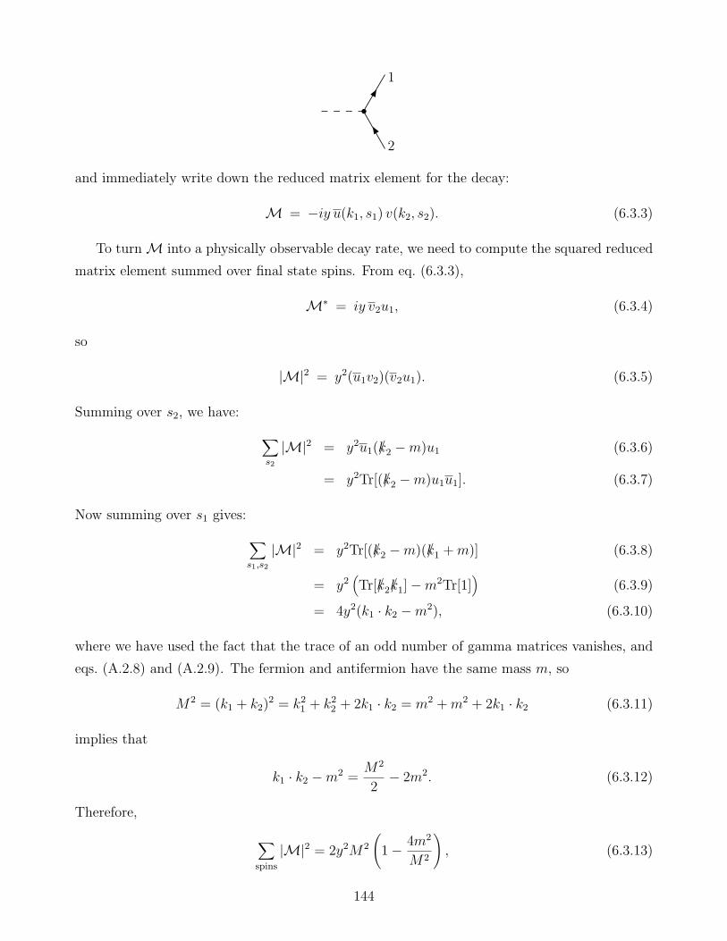
2

1

and immediately write down the reduced matrix element for the decay:

M = −iy u(k1, s1) v(k2, s2). (6.3.3)

To turnM into a physically observable decay rate, we need to compute the squared reduced

matrix element summed over final state spins. From eq. (6.3.3),

M∗ = iy v2u1, (6.3.4)

so

|M|2 = y2(u1v2)(v2u1). (6.3.5)

Summing over s2, we have:

∑

s2

|M|2 = y2u1(/k2 −m)u1 (6.3.6)

= y2Tr[(/k2 −m)u1u1]. (6.3.7)

Now summing over s1 gives:

∑

s1,s2

|M|2 = y2Tr[(/k2 −m)(/k1 +m)] (6.3.8)

= y2(Tr[/k2/k1]−m2Tr[1]

)(6.3.9)

= 4y2(k1 · k2 −m2), (6.3.10)

where we have used the fact that the trace of an odd number of gamma matrices vanishes, and

eqs. (A.2.8) and (A.2.9). The fermion and antifermion have the same mass m, so

M2 = (k1 + k2)2 = k21 + k22 + 2k1 · k2 = m2 +m2 + 2k1 · k2 (6.3.11)

implies that

k1 · k2 −m2 =M2

2− 2m2. (6.3.12)

Therefore,

∑

spins

|M|2 = 2y2M2

(1− 4m2

M2

), (6.3.13)

144

and, using eq. (6.2.11),

dΓ =y2M

32π2

(1− 4m2

M2

)3/2

dφ1 d(cos θ1). (6.3.14)

Doing the (trivial) angular integrals finally gives the total decay rate:

Γ =y2M

8π

(1− 4m2

M2

)3/2

. (6.3.15)

In the Standard Model, the Higgs boson h plays the role of φ, and couples to each fermion

f with a Lagrangian that is exactly of the form given above:

Lint = −∑

f

yf hΨfΨf . (6.3.16)

The Yukawa coupling for each fermion is approximately proportional to its mass:

yf ≈mf

175 GeV. (6.3.17)

(The reason for this will be explained below in section 11.3.) However, the mf appearing in this

formula is not quite equal to the mass, because of higher-order corrections. For quarks, these

corrections are quite large, and mf tends to come out considerably smaller than the masses of

the quarks quoted in Table 1.3.

At the LHC, one of the major goals is to study the Higgs boson through its decay modes.

The Higgs boson mass has been measured to be about 125 GeV. Since the top quark has a mass

of about 173 GeV, the decay h → tt is kinematically forbidden. The next-lightest fermions in

the Standard Model are the bottom quark, charm quark, and tau lepton, so we expect decays

h → bb and h → τ−τ+ and h → cc. For quarks, the sum in eq. (6.3.16) includes a summation

over 3 colors, leading to an extra factor of nf = 3 in the decay rate. Since the kinematic factor

(1− 4m2f/M

2h)

3/2 is close to 1 for all allowed fermion-antifermion final states, the leading-order

prediction for the decay rate to a particular fermion is approximately:

Γ(h→ ff) =nfy

2fMh

16π∝ nfm

2f . (6.3.18)

Estimates of the mf from present experimental data are:

mb ≈ 2.7 GeV → yb ≈ 0.0154, (6.3.19)

mτ ≈ 1.77 GeV → yτ ≈ 0.0101, (6.3.20)

mc ≈ 0.58 GeV → yc ≈ 0.0033, (6.3.21)

145

for a Higgs with mass Mh = 125 GeV. (Notice that even though the charm quark is heavier

than the tau lepton, it turns out that mτ > mc because of the large higher-order corrections for

the charm quark.) Therefore, the prediction is that bb final states win, with, very roughly:

Γ(h→ bb) : Γ(h→ τ−τ+) : Γ(h→ cc) :: 3(mb)2 : (mτ )

2 : 3(mc)2 (6.3.22)

:: 1 : 0.143 : 0.046. (6.3.23)

A more accurate accounting of the Higgs boson width and branching ratios must take into

account many important corrections beyond our scope here. For example, higher-order Feynman

diagram are important, and increase the partial widths into quarks substantially. Second, there

are other final states that can appear in h decays, notably gluon-gluon (gg) and γγ, which both

occur due to Feynman diagrams with loops, andW+W− and Z0Z0. Naively, the last two are not

kinematically allowed, since 2mW and 2mZ are both greater than mh. However, they can still

contribute if one or both of the weak vector bosons is off-shell (virtual). These decays are often

written as h → WW (∗) and h → ZZ(∗), with the (∗) indicating an off-shell particle. Normally,

such decays would be negligible compared to 2-body decays to on-shell particles, but they are

competitive because the bottom quark squared Yukawa coupling y2b ≈ 0.00024 is so small.

Taking into account these effects,† it turns out that the total width of the Higgs boson is

approximately 4.2MeV, assuming mh = 125 GeV. This is an extremely small decay width for

such a heavy particle. One can define the branching ratio to be the partial decay rate into a

particular final state, divided by the total decay rate, so for example

BR(h→ bb) = Γ(h→ bb)/Γtotal. (6.3.24)

In the Standard Model with mh = 125 GeV, the predicted branching fractions into b, τ , and c

pairs, taking into account all known effects, are:

BR(h→ bb) ≈ 0.577, (6.3.25)

BR(h→ τ−τ+) ≈ 0.063, (6.3.26)

BR(h→ cc) ≈ 0.029. (6.3.27)

Some other branching ratios that turn out to be extremely important for the Higgs boson at

the Large Hadron collider, but rely on more involved calculations, are:

BR(h→ WW (∗)) ≈ 0.215, (6.3.28)

BR(h→ ZZ(∗)) ≈ 0.0264, (6.3.29)

BR(h→ gg) ≈ 0.0857, (6.3.30)

BR(h→ γγ) ≈ 0.00228. (6.3.31)

†For the results quoted in this paragraph, see https://arxiv.org/abs/1307.1347 S. Heinemeyer et al., “Hand-book of LHC Higgs Cross Sections: 3. Higgs Properties”.

146

We will return to the subject of the Higgs boson branching ratios in section 11.5.

Finally, consider the helicities for the process h→ ff . If we demanded that the final states

have particular helicities, then we would have obtained for the matrix element, using PR, PL

projection matrices:

R-fermion, R-antifermion: M = −iy u2PLPLv1 = −iy u2PLv1 6= 0 (6.3.32)

L-fermion, L-antifermion: M = −iy u2PRPRv1 = −iy u2PRv1 6= 0 (6.3.33)

R-fermion, L-antifermion: M = −iy u2PLPRv1 = 0 (6.3.34)

L-fermion, R-antifermion: M = −iy u2PRPLv1 = 0 (6.3.35)

[Recall, from eqs. (5.2.63)-(5.2.66), that to get a L fermion or antifermion in the final state, one

puts in a PR next to the spinor, while to get a R fermion or antifermion in the final state, one puts

in a PL.] So, the rule here is that helicity is always violated by the scalar-fermion-antifermion

vertex, since the scalar must decay to a state with equal helicities.

One may understand this result from angular momentum conservation. The initial state had

no spin and no orbital angular momentum. In the final state, the spins of the outgoing particles

must therefore have opposite directions. Since they have momentum in opposite directions, this

means they must also have the same helicity. Drawing a short arrow to represent the spin, the

allowed cases of RR helicities and LL helicities look like:

R fermion R anti-fermionh

hL fermion L anti-fermion

The helicities of tau leptons can be (statistically) measured from the angular distributions of

their decay products, so this effect may eventually be measured with a sample of h → τ−τ+

decay events.

6.4 Three-body decays

Let us consider a generic three-body decay process in which a particle of massM decays to three

lighter particles with masses m1, m2, and m3. We will work in the rest frame of the decaying

particle, so its four-vector is pµ = (M, 0, 0, 0), and the four-vectors of the remaining particles

are k1, k2, and k3 respectively:

147

M

m1, k1

m3, k3m2, k2

In general, the formula for a three-body differential decay rate is

dΓ =1

2M|M|2dΦ3, (6.4.1)

where

dΦ3 = (2π)4δ(4)(p− k1 − k2 − k3)d3~k1

(2π)32E1

d3~k2(2π)32E2

d3~k3(2π)32E3

(6.4.2)

is the Lorentz-invariant phase space. Since there are 9 integrals to do, and 4 delta functions,

the result for dΓ is a differential with respect to 5 remaining variables. The best choice of 5

variables depends on the problem at hand, so there are several ways to present the result. Two

of the 5 variables can be chosen to be the energies E1 and E2 of two of the final-state particles;

then the energy of the third particle E3 =M −E1−E2 is also known from energy conservation.

In the rest frame of the decaying particle, the three final-state particle 3-momenta must lie in a

plane, because of momentum conservation. Specifying E1 and E2 also uniquely fixes the angles

between the three particle momenta within this decay plane. The remaining 3 variables just

correspond to the orientation of the decay plane with respect to some fixed coordinate axis. If

we think of the three 3-momenta within the decay plane as describing a rigid body, then the

relative orientation can be described using three Euler angles. These can be chosen to be the

spherical coordinate angles φ1 and θ1 for particle 1, and an angle α2 that measures the rotation

of the 3-momentum direction of particle 2 as measured about the axis of the momentum vector

of particle 1. Then one can show:

dΦ3 =1

256π5dE1 dE2 dφ1 d(cos θ1) dα2. (6.4.3)

The choice of which particles to label as 1 and 2 is arbitrary, and should be made to maximize

convenience.

If the initial state particle spin is averaged over, or if it is spinless, then there is no special

direction to measure the orientation of the final state decay plane with respect to. In that case,

for particular E1 and E2, the reduced matrix element cannot depend on the angles φ1, θ1, or

α2, and one can do the integrals∫ 2π

0dφ1

∫ 1

−1d(cos θ1)

∫ 2π

0dα2 = (2π)(2)(2π) = 8π2. (6.4.4)

148

Then,

dΦ3 =1

32π3dE1dE2, (6.4.5)

and so, for spinless or spin-averaged initial states,

dΓ =1

64π3M|M|2 dE1 dE2. (6.4.6)

To do the remaining energy integrals, one must find the limits of integration. If one decides to

do the E2 integral first, then by doing the kinematics one can show for any particular E1 that

Emax,min2 =

1

2m223

[(M − E1)(m

223 +m2

2 −m23)±

√(E2

1 −m21)λ(m

223,m

22,m

23)], (6.4.7)

where the triangle function λ(x, y, z) was defined by eq. (6.2.8), and

m223 = (k2 + k3)

2 = (p− k1)2 =M2 − 2E1M +m21 (6.4.8)

is the invariant (mass)2 of the combination of particles 2 and 3. Then the limits of integration

for the final E1 integral are:

m1 < E1 <M2 +m2

1 − (m2 +m3)2

2M. (6.4.9)

A good strategy is usually to choose the label “1” for the particle whose energy we care the

most about. Then after doing the dE2 integral, we will be left with an expression for dΓ/dE1.

In the special case that all final state particles are massless (or small enough to neglect)

m1 = m2 = m3 = 0, then these limits of integration simplify to:

M

2− E1 < E2 <

M

2, (6.4.10)

0 < E1 <M

2. (6.4.11)

149

7 Fermi Theory of Weak Interactions

7.1 Weak nuclear decays

In nuclear physics, the weak interactions are responsible for decays of long-lived isotopes. A nu-

cleus with Z protons and A−Z neutrons, so A nucleons in all, is denoted by AZ. If kinematically

allowed, one can observe decays:

AZ → A(Z + 1) + e−νe. (7.1.1)

The existence of the antineutrino νe was inferred by Pauli as a “desperate remedy” to save the

principle of energy conservation. The simplest example of this is the decay of the neutron into

a proton, electron, and antineutrino:

n→ p+e−νe (7.1.2)

with a mean lifetime of†

τ = 881.5± 1.5 sec. (7.1.3)

Decays of heavier nuclei can be thought of as involving the subprocess:

“n”→ “p+”e−νe, (7.1.4)

where the quotes indicated that the neutron and proton are really not separate entities, but

part of the nuclear bound states. So for example, tritium decays according to

3H→ 3He + e−νe (τ = 5.6× 108 sec = 17.7 years), (7.1.5)

and carbon-14 decays according to

14C→ 14N+ e−νe (τ = 1.8× 1011 sec = 8280 years). (7.1.6)

Nuclear physicists usually quote the half life t1/2 rather than the mean lifetime τ . They are

related by

t1/2 = τ ln(2), (7.1.7)

so that t1/2 = 5730 years for Carbon-14, making it ideal for dating dead organisms. In the upper

atmosphere, cosmic rays produce energetic neutrons, which in turn constantly convert 14N nuclei

†The lifetime of the neutron is an infamous example of an experimental measurement that has shifted dra-matically over time. As recently as the late 1960’s, it was thought that τn = 1010±30 seconds, and as recently as2010, the official value was 885.7± 0.8 seconds. Even today the systematic uncertainties are a source of concern.

150

into 14C. Carbon-dioxide-breathing organisms, or those that eat them, maintain an equilibrium

with the carbon content of the atmosphere, at a level of roughly 14C/12C≈ 10−12. However,

a complication is the fact that this ratio is not constant; it dropped in the early 20th century

as more ordinary 12C entered the atmosphere because of the burning of fossil fuels containing

the carbon of organisms that have been dead for a very long time. The relative abundance14C/12C≈ 10−12 then doubled after 1954 because of nuclear weapons testing, reaching a peak in

the mid 1960’s from which it has since declined. In any case, dead organisms lose half of their14C every 5730±30 years, and certainly do not regain it by breathing or eating. So, by measuring

the rate of e− beta rays consistent with 14C decay produced by a sample, and determining the

historic atmospheric 14C/12C ratio as a function of time with control samples or by other means,

one can date the death of a sample of organic matter.

One can also have decays that release a positron and neutrino:

AZ → A(Z − 1) + e+νe. (7.1.8)

These can be thought of as coming from the subprocess

“p+”→ “n”e+νe. (7.1.9)

In free space, the proton cannot decay, simply because mp < mn, but under the right circum-

stances it is kinematically allowed when the proton and neutron are parts of nuclear bound

states. An example is

14O→ 14N+ e+νe (τ = 71 sec). (7.1.10)

The long lifetimes of such decays are what originally gave rise to the name “weak” interactions.

Charged pions also decay through the weak interactions, with a mean lifetime of

τπ± = 2.6× 10−8 sec. (7.1.11)

This is still a very long lifetime by particle physics standards, and corresponds to a proper decay

length of cτ = 7.8 meters. The probability that a charged pion with velocity β will travel a

distance L in empty space before decaying is therefore

P = e−(L/7.8 m)√

1−β2/β. (7.1.12)

This means that a relativistic charged pion will typically travel several meters before decaying,

unless it interacts (which it usually will in a collider detector). The main decay mode is

π− → µ−νµ (7.1.13)

151

with a branching ratio of 0.99988. (This includes submodes in which an additional photon is

radiated away.) The only other significant decay mode is

π− → e−νe. (7.1.14)

with a branching ratio 1.2 × 10−4. This presents a puzzle: since the electron is lighter, there

is more kinematic phase space available for the second decay, yet the first decay dominates by

almost a factor of 104. We will calculate the reason for this later, in section 7.6.

7.2 Muon decay

The muon decays according to

µ− → e−νeνµ (τ = 2.2× 10−6 sec). (7.2.1)

This corresponds to a decay width of

Γ = 3.0× 10−19 GeV, (7.2.2)

implying a proper decay length of cτ = 659 meters. Muons do not undergo hadronic interactions

like pions do, so that relativistic muons will usually penetrate at least the inner layers of particle

detectors with a very high probability.

The Feynman diagram for muon decay can be drawn as:

µ−

e−

νe

νµ

This involves a 4-fermion interaction vertex.† Because of the correspondence between inter-

actions and terms in the Lagrangian, we therefore expect that the Lagrangian should contain

terms schematically of the form

Lint = (νµ . . . µ) (e . . . νe) or (νµ . . . νe) (e . . . µ), (7.2.3)

where the symbols µ, νµ, e, νe mean the Dirac spinor fields for the muon, muon neutrino, electron,

and electron neutrino, and the ellipses mean matrices in Dirac spinor space. To be more precise

about the interaction Lagrangian, one needs clues from experiment.

†We will later find out that this is not a true fundamental interaction of the theory, but rather an “effective”interaction that is derived from the low-energy effects of the W− boson.

152

One clue is the fact that there are three quantum numbers, called lepton numbers, that are

additively conserved to a high accuracy in most experiments. (The only confirmed exceptions

are neutrino oscillation experiments.) They are assigned as:

Le =

+1 for e−, νe−1 for e+, νe0 for all other particles

(7.2.4)

Lµ =

+1 for µ−, νµ−1 for µ+, νµ0 for all other particles

(7.2.5)

Lτ =

+1 for τ−, ντ−1 for τ+, ντ0 for all other particles

(7.2.6)

So, for example, in the nuclear decay examples above, one always has Le = 0 in the initial state,

and Le = 1− 1 = 0 in the final state, with Lµ = Lτ = 0 trivially in each case. The muon decay

mode in eq. (7.2.1) has (Le, Lµ) = (0, 1) in both the initial and final states. If lepton numbers

were not conserved, then one might expect that decays like

µ− → e−γ (7.2.7)

would be allowed. However, these decays have never been observed, and the most recent limit

from the MEG experiment at the Paul Scherrer Institute is

BR(µ− → e−γ) < 4.2× 10−13. (7.2.8)

(Actually, the MEG experiment searches for the decay µ+ → e+γ, but the branching ratio should

be the same with all particles replaced by their anti-particles.) This is a remarkably strong

constraint, since this decay only has to compete with the already weak mode in eq. (7.2.1). It

implies that

Γ(µ− → e−γ) < 1.3× 10−31 GeV. (7.2.9)

The BaBar and Belle experiments have put similar (but not as stringent) bounds on tau lepton

number non-conservation:

BR(τ− → e−γ) < 3.3× 10−8 BaBar, (7.2.10)

BR(τ− → µ−γ) < 4.4× 10−8 BaBar, (7.2.11)

BR(τ− → e−π0) < 8.0× 10−8 Belle. (7.2.12)

Since 1998, experimental results from neutrinos produced in the Sun, the atmosphere, by

accelerators, and in reactors have given strong evidence for oscillations of neutrinos that are

153

caused by them having small non-zero masses that violate the individual lepton numbers. (It is

still an open question whether they also violate the total lepton number

L ≡ Le + Lµ + Lτ ; (7.2.13)

for more on this, see section 11.4.) However, these are very small effects for colliding beam

experiments, and can be ignored for almost all conceivable processes at the Tevatron and the

LHC.

The (near) conservation of lepton numbers suggests that the interaction Lagrangian for the

weak interactions can always be written in terms of fermion bilinears involving one barred and

one unbarred Dirac spinor from each lepton family. So, we will write the weak interactions for

leptons in terms of building blocks with net Le = Lµ = Lτ = 0, for example, like the first term

in eq. (7.2.3) but not the second. More generally, we will want to use building blocks:

(ℓ . . . νℓ) or (νℓ . . . ℓ), (7.2.14)

where ℓ is any of e, µ, τ . Now, since each Dirac spinor has 4 components, a basis for fermion

bilinears involving any two fields Ψ1 and Ψ2 will have 4×4 = 16 elements. The can be classified

by their transformation properties under the proper Lorentz group and the parity transformation

~x→ −~x, as follows:

Term Number Parity (~x→ −~x) Type

Ψ1Ψ2 1 +1 Scalar = S

Ψ1γ5Ψ2 1 −1 Pseudo-scalar = P

Ψ1γµΨ2 4 (−1)µ Vector = V

Ψ1γµγ5Ψ2 4 −(−1)µ Axial-vector = A

i2Ψ1 [γ

µ, γν ] Ψ2 6 (−1)µ(−1)ν Tensor = T.

The entry under Parity indicates the multiplicative factor under which each of these terms

transforms when ~x→ −~x, with

(−1)µ =

+1 for µ = 0−1 for µ = 1, 2, 3.

(7.2.15)

The weak interaction Lagrangian for leptons could be formed out of any product of such terms

with Ψ1,Ψ2 = ℓ, νℓ. Fermi originally proposed that the weak interaction fermion building blocks

were of the type V , so that muon decays would be described by

LVint = −G(νµγρµ)(eγρνe) + c.c. (7.2.16)

Here “c.c.” means complex conjugate; this is necessary since the Dirac spinor fields are complex.

Some other possibilities could have been that the building blocks were of type A:

LAint = −G(νµγργ5µ)(eγργ5νe) + c.c. (7.2.17)

154

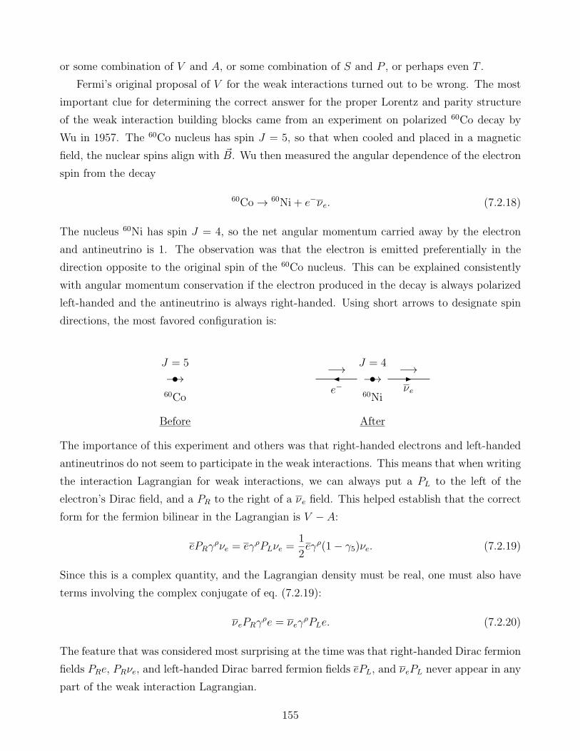
or some combination of V and A, or some combination of S and P , or perhaps even T .

Fermi’s original proposal of V for the weak interactions turned out to be wrong. The most

important clue for determining the correct answer for the proper Lorentz and parity structure

of the weak interaction building blocks came from an experiment on polarized 60Co decay by

Wu in 1957. The 60Co nucleus has spin J = 5, so that when cooled and placed in a magnetic

field, the nuclear spins align with ~B. Wu then measured the angular dependence of the electron

spin from the decay

60Co→ 60Ni + e−νe. (7.2.18)

The nucleus 60Ni has spin J = 4, so the net angular momentum carried away by the electron

and antineutrino is 1. The observation was that the electron is emitted preferentially in the

direction opposite to the original spin of the 60Co nucleus. This can be explained consistently

with angular momentum conservation if the electron produced in the decay is always polarized

left-handed and the antineutrino is always right-handed. Using short arrows to designate spin

directions, the most favored configuration is:

J = 5

−→60Co

Before

J = 4

−→60Ni

After

−→−→νee−

The importance of this experiment and others was that right-handed electrons and left-handed

antineutrinos do not seem to participate in the weak interactions. This means that when writing

the interaction Lagrangian for weak interactions, we can always put a PL to the left of the

electron’s Dirac field, and a PR to the right of a νe field. This helped establish that the correct

form for the fermion bilinear in the Lagrangian is V − A:

ePRγρνe = eγρPLνe =

1

2eγρ(1− γ5)νe. (7.2.19)

Since this is a complex quantity, and the Lagrangian density must be real, one must also have

terms involving the complex conjugate of eq. (7.2.19):

νePRγρe = νeγ

ρPLe. (7.2.20)

The feature that was considered most surprising at the time was that right-handed Dirac fermion

fields PRe, PRνe, and left-handed Dirac barred fermion fields ePL, and νePL never appear in any

part of the weak interaction Lagrangian.

155

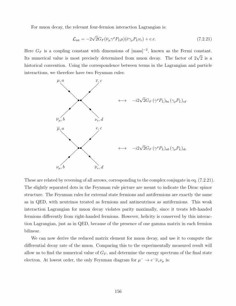
For muon decay, the relevant four-fermion interaction Lagrangian is:

Lint = −2√2GF (νµγ

ρPLµ)(eγρPLνe) + c.c. (7.2.21)

Here GF is a coupling constant with dimensions of [mass]−2, known as the Fermi constant.

Its numerical value is most precisely determined from muon decay. The factor of 2√2 is a

historical convention. Using the correspondence between terms in the Lagrangian and particle

interactions, we therefore have two Feynman rules:

µ, a e, c

νµ, b νe, d

←→ −i2√2GF (γρPL)ba (γρPL)cd

µ, a e, c

νµ, b νe, d

←→ −i2√2GF (γρPL)ab (γρPL)dc

These are related by reversing of all arrows, corresponding to the complex conjugate in eq. (7.2.21).

The slightly separated dots in the Feynman rule picture are meant to indicate the Dirac spinor

structure. The Feynman rules for external state fermions and antifermions are exactly the same

as in QED, with neutrinos treated as fermions and antineutrinos as antifermions. This weak

interaction Lagrangian for muon decay violates parity maximally, since it treats left-handed

fermions differently from right-handed fermions. However, helicity is conserved by this interac-

tion Lagrangian, just as in QED, because of the presence of one gamma matrix in each fermion

bilinear.

We can now derive the reduced matrix element for muon decay, and use it to compute the

differential decay rate of the muon. Comparing this to the experimentally measured result will

allow us to find the numerical value of GF , and determine the energy spectrum of the final state

electron. At lowest order, the only Feynman diagram for µ− → e−νeνµ is:

156

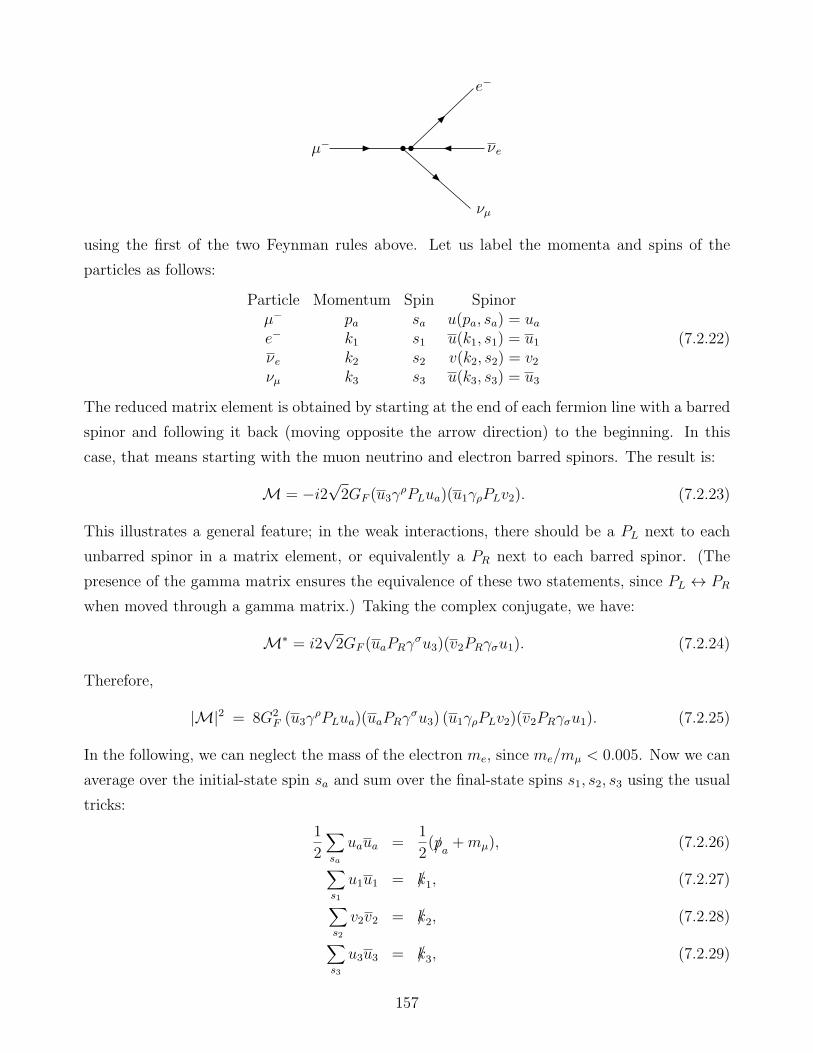
µ−

e−

νµ

νe

using the first of the two Feynman rules above. Let us label the momenta and spins of the

particles as follows:

Particle Momentum Spin Spinorµ− pa sa u(pa, sa) = uae− k1 s1 u(k1, s1) = u1νe k2 s2 v(k2, s2) = v2νµ k3 s3 u(k3, s3) = u3

(7.2.22)

The reduced matrix element is obtained by starting at the end of each fermion line with a barred

spinor and following it back (moving opposite the arrow direction) to the beginning. In this

case, that means starting with the muon neutrino and electron barred spinors. The result is:

M = −i2√2GF (u3γ

ρPLua)(u1γρPLv2). (7.2.23)

This illustrates a general feature; in the weak interactions, there should be a PL next to each

unbarred spinor in a matrix element, or equivalently a PR next to each barred spinor. (The

presence of the gamma matrix ensures the equivalence of these two statements, since PL ↔ PR

when moved through a gamma matrix.) Taking the complex conjugate, we have:

M∗ = i2√2GF (uaPRγ

σu3)(v2PRγσu1). (7.2.24)

Therefore,

|M|2 = 8G2F (u3γ

ρPLua)(uaPRγσu3) (u1γρPLv2)(v2PRγσu1). (7.2.25)

In the following, we can neglect the mass of the electron me, since me/mµ < 0.005. Now we can

average over the initial-state spin sa and sum over the final-state spins s1, s2, s3 using the usual

tricks:

1

2

∑

sa

uaua =1

2(/pa +mµ), (7.2.26)

∑

s1

u1u1 = /k1, (7.2.27)

∑

s2

v2v2 = /k2, (7.2.28)

∑

s3

u3u3 = /k3, (7.2.29)

157

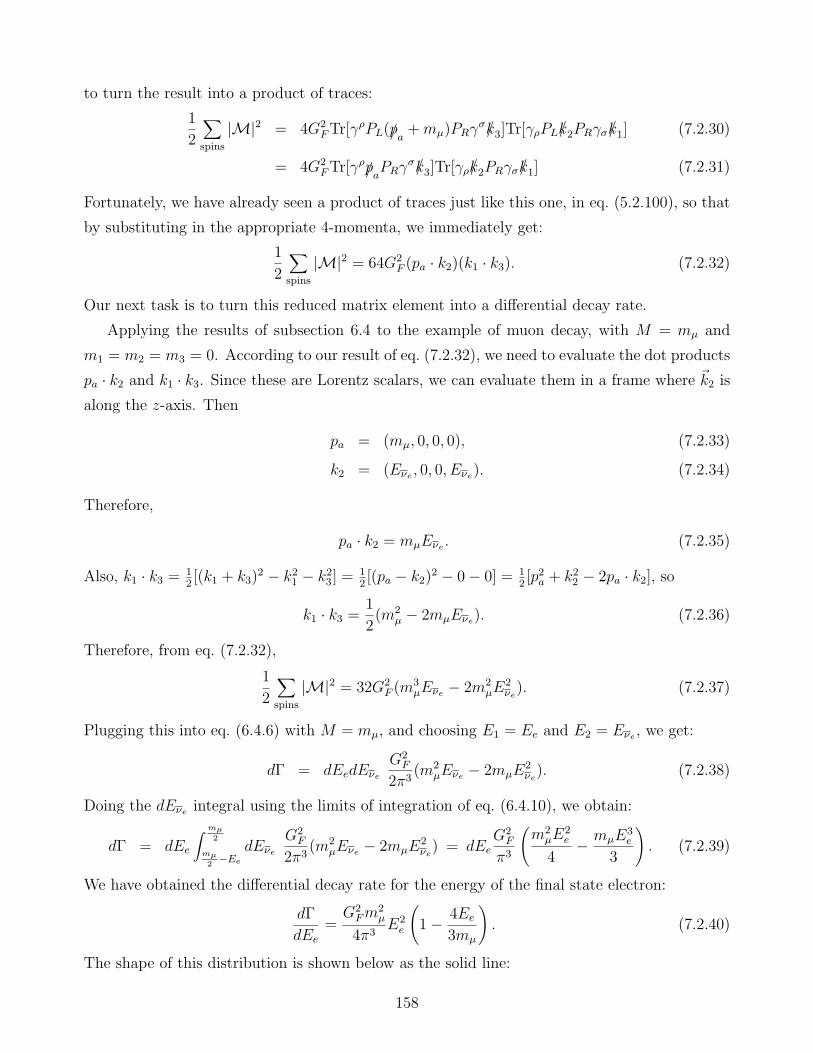
to turn the result into a product of traces:

1

2

∑

spins

|M|2 = 4G2FTr[γ

ρPL(/pa +mµ)PRγσ/k3]Tr[γρPL/k2PRγσ/k1] (7.2.30)

= 4G2FTr[γ

ρ/paPRγ

σ/k3]Tr[γρ/k2PRγσ/k1] (7.2.31)

Fortunately, we have already seen a product of traces just like this one, in eq. (5.2.100), so that

by substituting in the appropriate 4-momenta, we immediately get:

1

2

∑

spins

|M|2 = 64G2F (pa · k2)(k1 · k3). (7.2.32)

Our next task is to turn this reduced matrix element into a differential decay rate.

Applying the results of subsection 6.4 to the example of muon decay, with M = mµ and

m1 = m2 = m3 = 0. According to our result of eq. (7.2.32), we need to evaluate the dot products

pa · k2 and k1 · k3. Since these are Lorentz scalars, we can evaluate them in a frame where ~k2 is

along the z-axis. Then

pa = (mµ, 0, 0, 0), (7.2.33)

k2 = (Eνe , 0, 0, Eνe). (7.2.34)

Therefore,

pa · k2 = mµEνe . (7.2.35)

Also, k1 · k3 = 12[(k1 + k3)

2 − k21 − k23] = 12[(pa − k2)2 − 0− 0] = 1

2[p2a + k22 − 2pa · k2], so

k1 · k3 =1

2(m2

µ − 2mµEνe). (7.2.36)

Therefore, from eq. (7.2.32),

1

2

∑

spins

|M|2 = 32G2F (m

3µEνe − 2m2

µE2νe). (7.2.37)

Plugging this into eq. (6.4.6) with M = mµ, and choosing E1 = Ee and E2 = Eνe , we get:

dΓ = dEedEνe

G2F

2π3(m2

µEνe − 2mµE2νe). (7.2.38)

Doing the dEνe integral using the limits of integration of eq. (6.4.10), we obtain:

dΓ = dEe

∫ mµ

2

mµ

2−Ee

dEνe

G2F

2π3(m2

µEνe − 2mµE2νe) = dEe

G2F

π3

(m2

µE2e

4− mµE

3e

3

). (7.2.39)

We have obtained the differential decay rate for the energy of the final state electron:

dΓ

dEe

=G2

Fm2µ

4π3E2

e

(1− 4Ee

3mµ

). (7.2.40)

The shape of this distribution is shown below as the solid line:

158

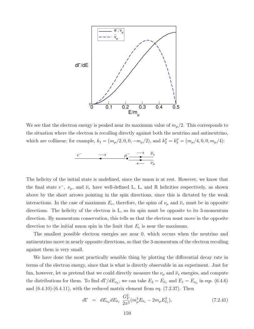
0 0.1 0.2 0.3 0.4 0.5E/mµ

0

dΓ/dE

e_, νµ

νe

We see that the electron energy is peaked near its maximum value of mµ/2. This corresponds to

the situation where the electron is recoiling directly against both the neutrino and antineutrino,

which are collinear; for example, k1 = (mµ/2, 0, 0,−mµ/2), and kµ2 = kµ3 = (mµ/4, 0, 0,mµ/4):

µ−e− −→ −→

←− νµ

νe

The helicity of the initial state is undefined, since the muon is at rest. However, we know that

the final state e−, νµ, and νe have well-defined L, L, and R helicities respectively, as shown

above by the short arrows pointing in the spin directions, since this is dictated by the weak

interactions. In the case of maximum Ee, therefore, the spins of νµ and νe must be in opposite

directions. The helicity of the electron is L, so its spin must be opposite to its 3-momentum

direction. By momentum conservation, this tells us that the electron must move in the opposite

direction to the initial muon spin in the limit that Ee is near the maximum.

The smallest possible electron energies are near 0, which occurs when the neutrino and

antineutrino move in nearly opposite directions, so that the 3-momentum of the electron recoiling

against them is very small.

We have done the most practically sensible thing by plotting the differential decay rate in

terms of the electron energy, since that is what is directly observable in an experiment. Just for

fun, however, let us pretend that we could directly measure the νµ and νe energies, and compute

the distributions for them. To find dΓ/dEνµ , we can take E2 = Eνe and E1 = Eνµ in eqs. (6.4.6)

and (6.4.10)-(6.4.11), with the reduced matrix element from eq. (7.2.37). Then

dΓ = dEνµdEνe

G2F

2π3(m2

µEνe − 2mµE2νe), (7.2.41)

159

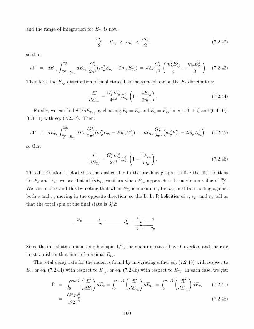
and the range of integration for Eνe is now:

mµ

2− Eνµ < Eνe <

mµ

2, (7.2.42)

so that

dΓ = dEνµ

∫ mµ

2

mµ

2−Eνµ

dEνe

G2F

2π3(m2

µEνe − 2mµE2νe) = dEe

G2F

π3

(m2

µE2νµ

4−mµE

3νµ

3

). (7.2.43)

Therefore, the Eνµ distribution of final states has the same shape as the Ee distribution:

dΓ

dEνµ

=G2

Fm2µ

4π3E2

νµ

(1− 4Eνµ

3mµ

). (7.2.44)

Finally, we can find dΓ/dEνe , by choosing E2 = Ee and E1 = Eνe in eqs. (6.4.6) and (6.4.10)-

(6.4.11) with eq. (7.2.37). Then:

dΓ = dEνe

∫ mµ

2

mµ

2−Eνe

dEeG2

F

2π3(m2

µEνe − 2mµE2νe) = dEνe

G2F

2π3

(m2

µE2νe − 2mµE

3νe

), (7.2.45)

so that

dΓ

dEνe

=G2

Fm2µ

2π3E2

νe

(1− 2Eνe

mµ

). (7.2.46)

This distribution is plotted as the dashed line in the previous graph. Unlike the distributions

for Ee and Eν , we see that dΓ/dEνe vanishes when Eνe approaches its maximum value of mµ

2.

We can understand this by noting that when Eνe is maximum, the νe must be recoiling against

both e and νe moving in the opposite direction, so the L, L, R helicities of e, νµ, and νe tell us

that the total spin of the final state is 3/2:

µ−νe ←− ←−

←− νµ

e

Since the initial-state muon only had spin 1/2, the quantum states have 0 overlap, and the rate

must vanish in that limit of maximal Eνe .

The total decay rate for the muon is found by integrating either eq. (7.2.40) with respect to

Ee, or eq. (7.2.44) with respect to Eνµ , or eq. (7.2.46) with respect to Eνe . In each case, we get:

Γ =∫ mµ/2

0

(dΓ

dEe

)dEe =

∫ mµ/2

0

(dΓ

dEνµ

)dEνµ =

∫ mµ/2

0

(dΓ

dEνe

)dEνe (7.2.47)

=G2

Fm5µ

192π3. (7.2.48)

160

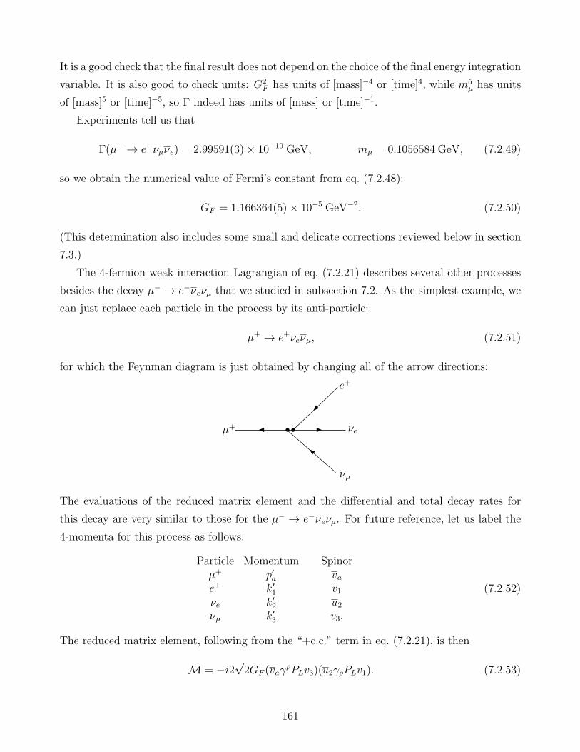
It is a good check that the final result does not depend on the choice of the final energy integration

variable. It is also good to check units: G2F has units of [mass]−4 or [time]4, while m5

µ has units

of [mass]5 or [time]−5, so Γ indeed has units of [mass] or [time]−1.

Experiments tell us that

Γ(µ− → e−νµνe) = 2.99591(3)× 10−19 GeV, mµ = 0.1056584 GeV, (7.2.49)

so we obtain the numerical value of Fermi’s constant from eq. (7.2.48):

GF = 1.166364(5)× 10−5 GeV−2. (7.2.50)

(This determination also includes some small and delicate corrections reviewed below in section

7.3.)

The 4-fermion weak interaction Lagrangian of eq. (7.2.21) describes several other processes

besides the decay µ− → e−νeνµ that we studied in subsection 7.2. As the simplest example, we

can just replace each particle in the process by its anti-particle:

µ+ → e+νeνµ, (7.2.51)

for which the Feynman diagram is just obtained by changing all of the arrow directions:

µ+

e+

νµ

νe

The evaluations of the reduced matrix element and the differential and total decay rates for

this decay are very similar to those for the µ− → e−νeνµ. For future reference, let us label the

4-momenta for this process as follows:

Particle Momentum Spinorµ+ p′a vae+ k′1 v1νe k′2 u2νµ k′3 v3.

(7.2.52)

The reduced matrix element, following from the “+c.c.” term in eq. (7.2.21), is then

M = −i2√2GF (vaγ

ρPLv3)(u2γρPLv1). (7.2.53)

161

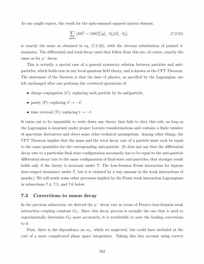
As one might expect, the result for the spin-summed squared matrix element,

∑

spins

|M|2 = 128G2F (p

′a · k′2)(k′1 · k′3), (7.2.54)

is exactly the same as obtained in eq. (7.2.32), with the obvious substitution of primed 4-

momenta. The differential and total decay rates that follow from this are, of course, exactly the

same as for µ− decay.

This is actually a special case of a general symmetry relation between particles and anti-

particles, which holds true in any local quantum field theory, and is known as the CPT Theorem.

The statement of the theorem is that the laws of physics, as specified by the Lagrangian, are

left unchanged after one performs the combined operations of:

• charge conjugation (C): replacing each particle by its antiparticle,

• parity (P): replacing ~x→ −~x,

• time reversal (T): replacing t→ −t.

It turns out to be impossible to write down any theory that fails to obey this rule, as long as

the Lagrangian is invariant under proper Lorentz transformations and contains a finite number

of spacetime derivatives and obeys some other technical assumptions. Among other things, the

CPT Theorem implies that the mass and the total decay rate of a particle must each be equal

to the same quantities for the corresponding anti-particle. (It does not say that the differential

decay rate to a particular final state configuration necessarily has to be equal to the anti-particle

differential decay rate to the same configuration of final-state anti-particles; that stronger result

holds only if the theory is invariant under T. The four-fermion Fermi interaction for leptons

does respect invariance under T, but it is violated by a tiny amount in the weak interactions of

quarks.) We will study some other processes implied by the Fermi weak interaction Lagrangians

in subsections 7.4, 7.5, and 7.6 below.

7.3 Corrections to muon decay

In the previous subsection, we derived the µ− decay rate in terms of Fermi’s four-fermion weak

interaction coupling constant GF . Since this decay process is actually the one that is used to

experimentally determine GF most accurately, it is worthwhile to note the leading corrections

to it.

First, there is the dependence on me, which we neglected, but could have included at the

cost of a more complicated phase space integration. Taking this into account using correct

162

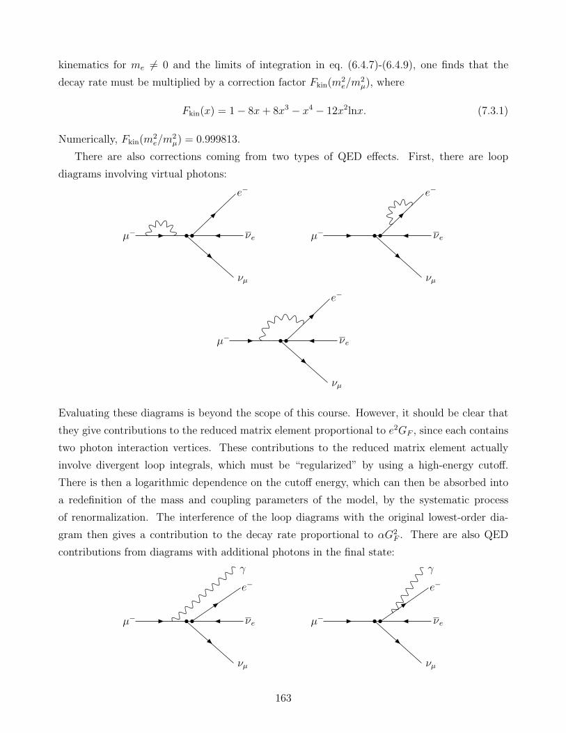
kinematics for me 6= 0 and the limits of integration in eq. (6.4.7)-(6.4.9), one finds that the

decay rate must be multiplied by a correction factor Fkin(m2e/m

2µ), where

Fkin(x) = 1− 8x+ 8x3 − x4 − 12x2lnx. (7.3.1)

Numerically, Fkin(m2e/m

2µ) = 0.999813.

There are also corrections coming from two types of QED effects. First, there are loop

diagrams involving virtual photons:

µ−

e−

νµ

νe µ−

e−

νµ

νe

µ−

e−

νµ

νe

Evaluating these diagrams is beyond the scope of this course. However, it should be clear that

they give contributions to the reduced matrix element proportional to e2GF , since each contains

two photon interaction vertices. These contributions to the reduced matrix element actually

involve divergent loop integrals, which must be “regularized” by using a high-energy cutoff.

There is then a logarithmic dependence on the cutoff energy, which can then be absorbed into

a redefinition of the mass and coupling parameters of the model, by the systematic process

of renormalization. The interference of the loop diagrams with the original lowest-order dia-

gram then gives a contribution to the decay rate proportional to αG2F . There are also QED

contributions from diagrams with additional photons in the final state:

µ−

γ

e−

νµ

νe µ−

γ

e−

νµ

νe

163

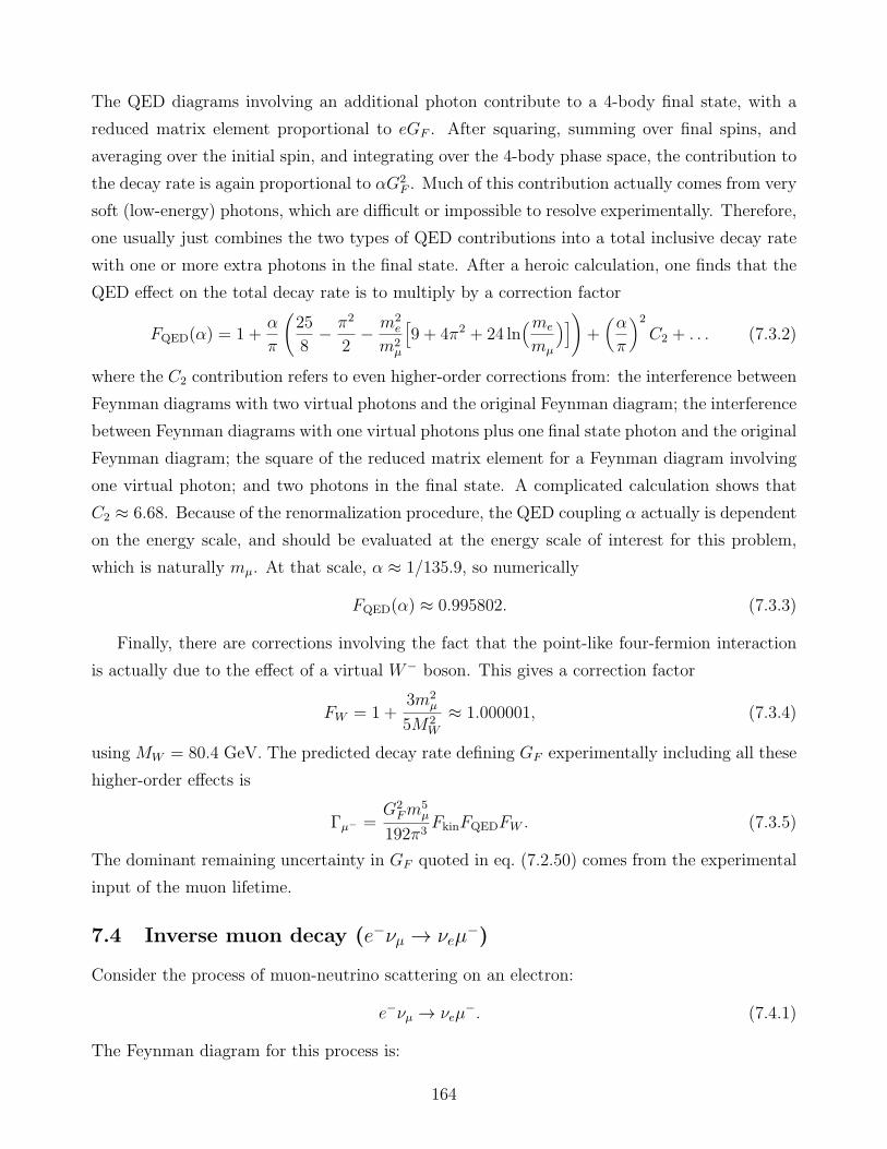
The QED diagrams involving an additional photon contribute to a 4-body final state, with a

reduced matrix element proportional to eGF . After squaring, summing over final spins, and

averaging over the initial spin, and integrating over the 4-body phase space, the contribution to

the decay rate is again proportional to αG2F . Much of this contribution actually comes from very

soft (low-energy) photons, which are difficult or impossible to resolve experimentally. Therefore,

one usually just combines the two types of QED contributions into a total inclusive decay rate

with one or more extra photons in the final state. After a heroic calculation, one finds that the

QED effect on the total decay rate is to multiply by a correction factor

FQED(α) = 1 +α

π

(25

8− π2

2− m2

e

m2µ

[9 + 4π2 + 24 ln

(me

mµ

)])+(α

π

)2

C2 + . . . (7.3.2)

where the C2 contribution refers to even higher-order corrections from: the interference between

Feynman diagrams with two virtual photons and the original Feynman diagram; the interference

between Feynman diagrams with one virtual photons plus one final state photon and the original

Feynman diagram; the square of the reduced matrix element for a Feynman diagram involving

one virtual photon; and two photons in the final state. A complicated calculation shows that

C2 ≈ 6.68. Because of the renormalization procedure, the QED coupling α actually is dependent

on the energy scale, and should be evaluated at the energy scale of interest for this problem,

which is naturally mµ. At that scale, α ≈ 1/135.9, so numerically

FQED(α) ≈ 0.995802. (7.3.3)

Finally, there are corrections involving the fact that the point-like four-fermion interaction

is actually due to the effect of a virtual W− boson. This gives a correction factor

FW = 1 +3m2

µ

5M2W

≈ 1.000001, (7.3.4)

using MW = 80.4 GeV. The predicted decay rate defining GF experimentally including all these

higher-order effects is

Γµ− =G2

Fm5µ

192π3FkinFQEDFW . (7.3.5)

The dominant remaining uncertainty in GF quoted in eq. (7.2.50) comes from the experimental

input of the muon lifetime.

7.4 Inverse muon decay (e−νµ → νeµ−)

Consider the process of muon-neutrino scattering on an electron:

e−νµ → νeµ−. (7.4.1)

The Feynman diagram for this process is:

164

e−, pa νe, k1

νµ, pb µ−, k2

in which we see that the following particles have been crossed from the previous diagram for µ+

decay:

initial µ+ → final µ− (7.4.2)

final e+ → initial e− (7.4.3)

final νµ → initial νµ. (7.4.4)

In fact, this scattering process is often known as inverse muon decay. To apply the Crossing

Symmetry Theorem stated in section 5.3, we can assign momentum labels pa, pb, k1, k2 to e−,

νµ, νe, µ− respectively, as shown in the figure, and then make the following comparison table:

µ+ → e+νeνµ e−νµ → νeµ−

µ+, p′a µ−, k2

e+, k′1 e−, pa

νe, k′2 νe, k1

νµ, k′3 νµ, pb

(7.4.5)

Therefore, we obtain the spin-summed, squared matrix element for e−νµ → νeµ− by making the

replacements

p′a = −k2; k′1 = −pa; k′2 = k1; k′3 = −pb (7.4.6)

in eq. (7.2.54), and then multiplying by (−1)3 for three crossed fermions, resulting in:

∑

spins

|Me−νµ→νeµ− |2 = 128G2F (k2 · k1)(pa · pb). (7.4.7)

Let us evaluate this result in the limit of high-energy scattering, so that mµ can be neglected,

and in the center-of-momentum frame. In that case, all four particles being treated as massless,

we can take the kinematics results from eqs. (5.2.139)-(5.2.143), so that pa · pb = k1 · k2 = s/2,

and

∑

spins

|Me−νµ→νeµ− |2 = 32G2F s

2. (7.4.8)

165

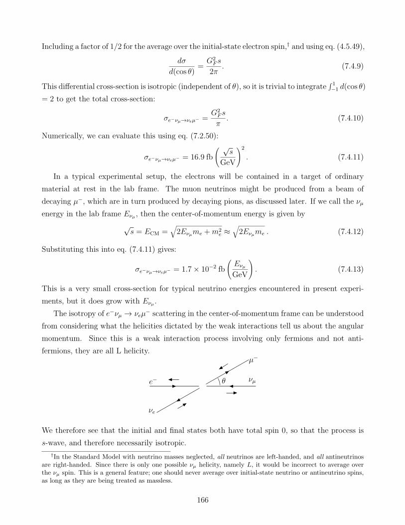
Including a factor of 1/2 for the average over the initial-state electron spin,† and using eq. (4.5.49),

dσ

d(cos θ)=G2

F s

2π. (7.4.9)

This differential cross-section is isotropic (independent of θ), so it is trivial to integrate∫ 1−1 d(cos θ)

= 2 to get the total cross-section:

σe−νµ→νeµ− =G2

F s

π. (7.4.10)

Numerically, we can evaluate this using eq. (7.2.50):

σe−νµ→νeµ− = 16.9 fb

( √s

GeV

)2

. (7.4.11)

In a typical experimental setup, the electrons will be contained in a target of ordinary

material at rest in the lab frame. The muon neutrinos might be produced from a beam of

decaying µ−, which are in turn produced by decaying pions, as discussed later. If we call the νµ

energy in the lab frame Eνµ , then the center-of-momentum energy is given by

√s = ECM =

√2Eνµme +m2

e ≈√2Eνµme . (7.4.12)

Substituting this into eq. (7.4.11) gives:

σe−νµ→νeµ− = 1.7× 10−2 fb

(Eνµ

GeV

). (7.4.13)

This is a very small cross-section for typical neutrino energies encountered in present experi-

ments, but it does grow with Eνµ .

The isotropy of e−νµ → νeµ− scattering in the center-of-momentum frame can be understood

from considering what the helicities dictated by the weak interactions tell us about the angular

momentum. Since this is a weak interaction process involving only fermions and not anti-

fermions, they are all L helicity.

e− νµ

νe

µ−

θ

We therefore see that the initial and final states both have total spin 0, so that the process is

s-wave, and therefore necessarily isotropic.

†In the Standard Model with neutrino masses neglected, all neutrinos are left-handed, and all antineutrinosare right-handed. Since there is only one possible νµ helicity, namely L, it would be incorrect to average overthe νµ spin. This is a general feature; one should never average over initial-state neutrino or antineutrino spins,as long as they are being treated as massless.

166

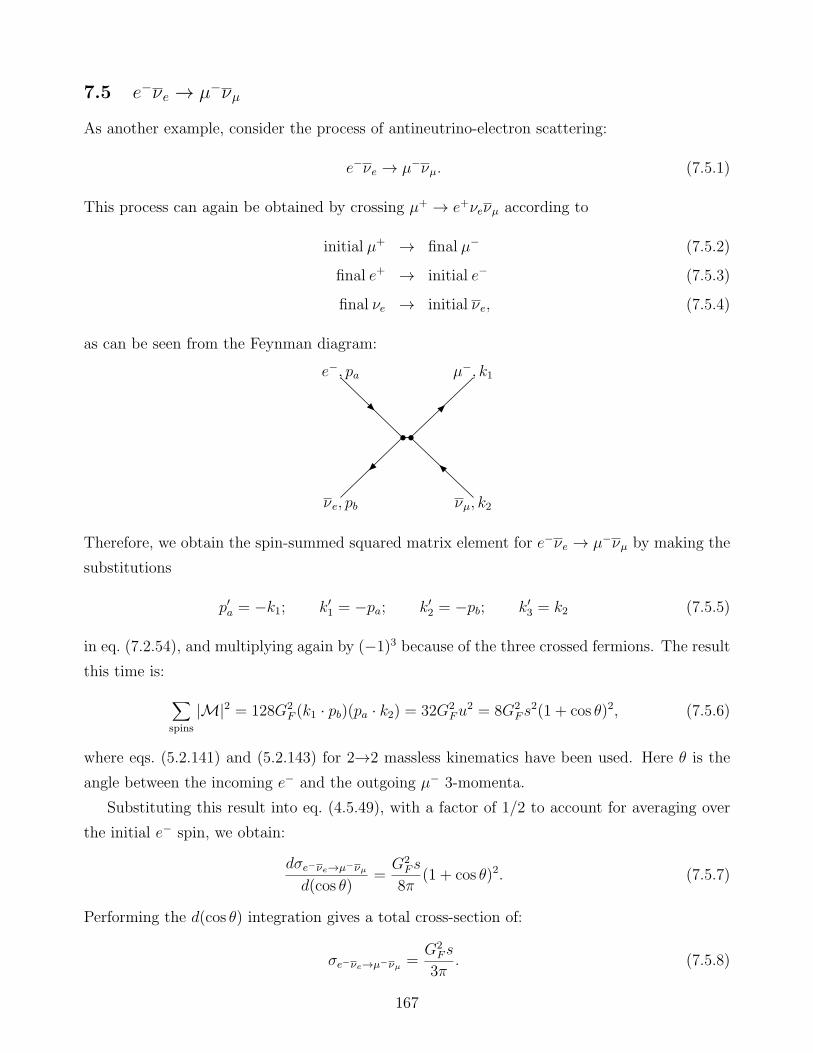
7.5 e−νe → µ−νµ

As another example, consider the process of antineutrino-electron scattering:

e−νe → µ−νµ. (7.5.1)

This process can again be obtained by crossing µ+ → e+νeνµ according to

initial µ+ → final µ− (7.5.2)

final e+ → initial e− (7.5.3)

final νe → initial νe, (7.5.4)

as can be seen from the Feynman diagram:

e−, pa µ−, k1

νe, pb νµ, k2

Therefore, we obtain the spin-summed squared matrix element for e−νe → µ−νµ by making the

substitutions

p′a = −k1; k′1 = −pa; k′2 = −pb; k′3 = k2 (7.5.5)

in eq. (7.2.54), and multiplying again by (−1)3 because of the three crossed fermions. The result

this time is:

∑

spins

|M|2 = 128G2F (k1 · pb)(pa · k2) = 32G2

Fu2 = 8G2

F s2(1 + cos θ)2, (7.5.6)

where eqs. (5.2.141) and (5.2.143) for 2→2 massless kinematics have been used. Here θ is the

angle between the incoming e− and the outgoing µ− 3-momenta.

Substituting this result into eq. (4.5.49), with a factor of 1/2 to account for averaging over

the initial e− spin, we obtain:

dσe−νe→µ−νµ

d(cos θ)=G2

F s

8π(1 + cos θ)2. (7.5.7)

Performing the d(cos θ) integration gives a total cross-section of:

σe−νe→µ−νµ =G2

F s

3π. (7.5.8)

167

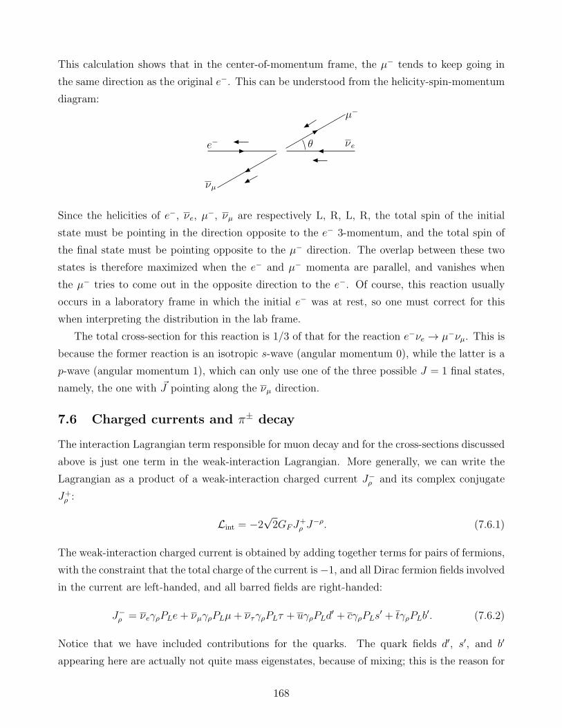
This calculation shows that in the center-of-momentum frame, the µ− tends to keep going in

the same direction as the original e−. This can be understood from the helicity-spin-momentum

diagram:

e− νe

νµ

µ−

θ

Since the helicities of e−, νe, µ−, νµ are respectively L, R, L, R, the total spin of the initial

state must be pointing in the direction opposite to the e− 3-momentum, and the total spin of

the final state must be pointing opposite to the µ− direction. The overlap between these two

states is therefore maximized when the e− and µ− momenta are parallel, and vanishes when

the µ− tries to come out in the opposite direction to the e−. Of course, this reaction usually

occurs in a laboratory frame in which the initial e− was at rest, so one must correct for this

when interpreting the distribution in the lab frame.

The total cross-section for this reaction is 1/3 of that for the reaction e−νe → µ−νµ. This is

because the former reaction is an isotropic s-wave (angular momentum 0), while the latter is a

p-wave (angular momentum 1), which can only use one of the three possible J = 1 final states,

namely, the one with ~J pointing along the νµ direction.

7.6 Charged currents and π± decay

The interaction Lagrangian term responsible for muon decay and for the cross-sections discussed

above is just one term in the weak-interaction Lagrangian. More generally, we can write the

Lagrangian as a product of a weak-interaction charged current J−ρ and its complex conjugate

J+ρ :

Lint = −2√2GFJ

+ρ J

−ρ. (7.6.1)

The weak-interaction charged current is obtained by adding together terms for pairs of fermions,

with the constraint that the total charge of the current is−1, and all Dirac fermion fields involved

in the current are left-handed, and all barred fields are right-handed:

J−ρ = νeγρPLe+ νµγρPLµ+ ντγρPLτ + uγρPLd

′ + cγρPLs′ + tγρPLb

′. (7.6.2)

Notice that we have included contributions for the quarks. The quark fields d′, s′, and b′

appearing here are actually not quite mass eigenstates, because of mixing; this is the reason for

168

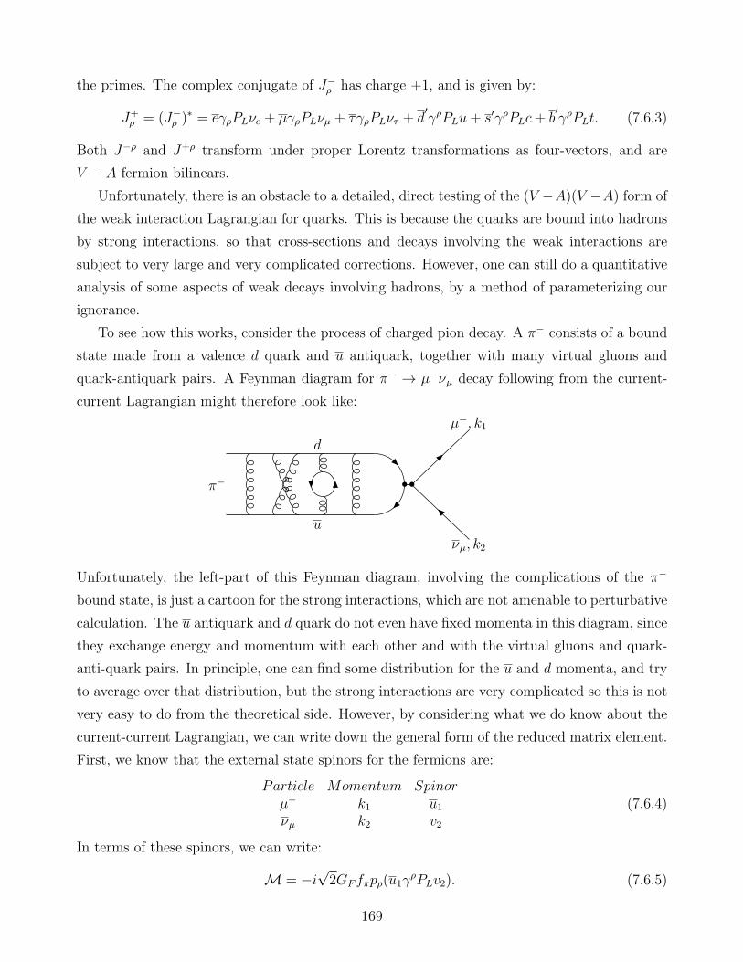
the primes. The complex conjugate of J−ρ has charge +1, and is given by:

J+ρ = (J−

ρ )∗ = eγρPLνe + µγρPLνµ + τγρPLντ + d

′γρPLu+ s′γρPLc+ b

′γρPLt. (7.6.3)

Both J−ρ and J+ρ transform under proper Lorentz transformations as four-vectors, and are

V − A fermion bilinears.

Unfortunately, there is an obstacle to a detailed, direct testing of the (V −A)(V −A) form of

the weak interaction Lagrangian for quarks. This is because the quarks are bound into hadrons

by strong interactions, so that cross-sections and decays involving the weak interactions are

subject to very large and very complicated corrections. However, one can still do a quantitative

analysis of some aspects of weak decays involving hadrons, by a method of parameterizing our

ignorance.

To see how this works, consider the process of charged pion decay. A π− consists of a bound

state made from a valence d quark and u antiquark, together with many virtual gluons and

quark-antiquark pairs. A Feynman diagram for π− → µ−νµ decay following from the current-

current Lagrangian might therefore look like:

µ−, k1

νµ, k2

π−

u

d

Unfortunately, the left-part of this Feynman diagram, involving the complications of the π−

bound state, is just a cartoon for the strong interactions, which are not amenable to perturbative

calculation. The u antiquark and d quark do not even have fixed momenta in this diagram, since

they exchange energy and momentum with each other and with the virtual gluons and quark-

anti-quark pairs. In principle, one can find some distribution for the u and d momenta, and try

to average over that distribution, but the strong interactions are very complicated so this is not

very easy to do from the theoretical side. However, by considering what we do know about the

current-current Lagrangian, we can write down the general form of the reduced matrix element.

First, we know that the external state spinors for the fermions are:

Particle Momentum Spinorµ− k1 u1νµ k2 v2

(7.6.4)

In terms of these spinors, we can write:

M = −i√2GFfπpρ(u1γ

ρPLv2). (7.6.5)

169

In this formula, the factor (u1γρPLv2) just reflects the fact that leptons are immune from the

complications of the strong interactions. The factor fπpρ takes into account the part of the

reduced matrix element involving the π−; here pρ is the 4-momentum of the pion. The point is

that whatever the pion factor in the reduced matrix element is, we know that it is a four-vector in

order to contract with the lepton part, and it must be proportional to pρ, since there is no other

vector quantity in the problem that it can depend on. (Recall that pions are spinless, so there

is no spin dependence.) So we are simply parameterizing all of our ignorance of the bound-state

properties of the pion in terms of a single constant fπ, called the pion decay constant. It is a

quantity with dimensions of mass. In principle we could compute it if we had perfect ability to

calculate with the strong interactions. In practice, fπ is an experimentally measured quantity,

with its value following most accurately from the π− lifetime that we will compute below. The

factor√2GF is another historical convention; it could have been absorbed into the definition of

fπ. But it is useful to have the GF appear explicitly as a sign that this is a weak interaction;

then fπ is entirely a strong-interaction parameter.

Let us now compute the decay rate for π− → µ−νµ. Taking the complex square of the

reduced matrix element eq. (7.6.5), we have:

|M|2 = 2G2Ff

2πpρpσ(u1γ

ρPLv2)(v2PRγσu1). (7.6.6)

Now summing over final state spins in the usual way gives:

∑

spins

|M|2 = 2G2Ff

2πpρpσTr[γ

ρPL/k2PRγσ(/k1 +mµ)] = 2G2

Ff2πTr[/p/k2PR/p/k1]. (7.6.7)

Note that we do not neglect the mass of the muon, since mµ/mπ± = 0.1056 GeV/0.1396 GeV

= 0.756 is not a small number. However, the term in eq. (7.6.7) that explicitly involves mµ does

not contribute, since the trace of 3 gamma matrices (with or without a PR) vanishes. Evaluating

the trace, we have:

Tr[/p/k2PR/p/k1] = 4(p · k1)(p · k2)− 2p2(k1 · k2). (7.6.8)

The decay kinematics tells us that:

p2 = m2π± ; k21 = m2

µ; k22 = m2νµ = 0; (7.6.9)

p · k1 =1

2[−(p− k1)2 + p2 + k21] =

1

2(m2

π± +m2µ); (7.6.10)

p · k2 =1

2[−(p− k2)2 + p2 + k22] =

1

2(−m2

µ +m2π±); (7.6.11)

k1 · k2 =1

2[(k1 + k2)

2 − k21 − k22] =1

2(m2

π± −m2µ). (7.6.12)

170

Therefore, Tr[/p/k2PR/p/k1] = m2µ(m

2π± −m2

µ), and

∑

spins

|M|2 = 2G2Ff

2πm

2π±m2

µ

(1− m2

µ

m2π±

), (7.6.13)

so that using eq. (6.2.14), we get:

dΓ =G2

Ff2πmπ±m2

µ

32π2

(1− m2

µ

m2π±

)2

dφ d(cos θ), (7.6.14)

where (θ, φ) are the angles for the µ− three-momentum. Of course, since the pion is spinless,

the differential decay rate is isotropic, so the angular integration trivially gives dφd(cos θ)→ 4π,

and:

Γ(π− → µ−νµ) =G2

Ff2πmπ±m2

µ

8π

(1− m2

µ

m2π±

)2

. (7.6.15)

The charged pion can also decay according to π− → e−νe. The calculation of this decay rate

is identical to the one just given, except that me is substituted everywhere for mµ. Therefore,

we have:

Γ(π− → e−νe) =G2

Ff2πmπ±m2

e

8π

(1− m2

e

m2π±

)2

, (7.6.16)

and the ratio of branching ratios is predicted to be:

BR(π− → e−νe)

BR(π− → µ−νµ)=

Γ(π− → e−νe)

Γ(π− → µ−νµ)=

(m2

e

m2µ

)(m2

π± −m2e

m2π± −m2

µ

)2

= 1.2× 10−4. (7.6.17)

The ratio eq. (7.6.17) is a robust prediction of the theory, because the dependence on fπ has

canceled out. Since there are no other kinematically-possible two-body decay channels open to

π−, it should decay to µ−νµ almost always, with a rare decay to e−νe occurring 0.012% of the

time. This has been confirmed experimentally. We can also use the measurement of the total

lifetime of the π− to find fπ numerically, using eq. (7.6.15). The result is:

fπ = 0.128 GeV. (7.6.18)

It is not surprising that this value is of the same order-of-magnitude as the mass of the pion.

The most striking feature of the π− decay rate is that it is proportional to m2µ, with M

proportional to mµ. This is what leads to the strong suppression of decays to e−νe (already

mentioned at the end of section 7.1). We found this result just by calculating. To understand

it better, we can draw a momentum-helicity-spin diagram, using the fact that the ℓ− and νℓ

produced in the weak interactions are L and R respectively:

171

J = 0

π−

−→−→νee

The π− has spin 0, but the final state predicted by the weak interaction helicities unambiguously

has spin 1. Therefore, if helicity were exactly conserved, the π− could not decay at all! However,

helicity conservation only holds in the high-energy limit in which we can treat all fermions as

massless. This decay is said to be helicity-suppressed, since the only reason it can occur is

because mµ and me are non-zero. In the limit mℓ → 0, we recover exact helicity conservation

and the reduced matrix element and the decay lifetime vanish. This explains why they should

be proportional to mℓ and m2ℓ respectively. The helicity suppression of this decay is therefore a

good prediction of the rule that the weak interactions affect only L fermions and R antifermions.

In the final state, the charged lepton µ− or e− is said to undergo a helicity flip, meaning that the

L-helicity fermion produced by the weak interactions has an amplitude to appear in the final

state as a R-fermion. In general, a helicity flip for a fermion entails a suppression in the reduced

matrix element proportional to the mass of the fermion divided by its energy.

Having computed the decay rate following from eq. (7.6.5), let us find a Lagrangian that

would give rise to it involving a quantum field for the pion. Although the pion is a composite,

bound-state particle, we can still invent a quantum field for it, in an approximate, “effective”

description. The π− corresponds to a charged spin-0 field. Previously, we studied spin-0 particles

described by a real scalar field. However, the particle and antiparticle created by a real scalar

field turned out to be the same thing. Here we want something different; since the π− is charged,

its antiparticle π+ is clearly a different particle. This means that the π− particle should be

described by a complex scalar field.

Let us therefore define π−(x) to be a complex scalar field, with its complex conjugate given

by

π+(x) ≡ (π−(x))∗. (7.6.19)

We can construct a real free Lagrangian density from these complex fields as follows:

L = ∂µπ+∂µπ− −m2

π±π+π−. (7.6.20)

[Compare to the Lagrangian density for a real scalar field, eq. (4.1.18).] This Lagrangian density

describes free pion fields with mass mπ± . At any fixed time t = 0, the π+ and π− fields can be

172

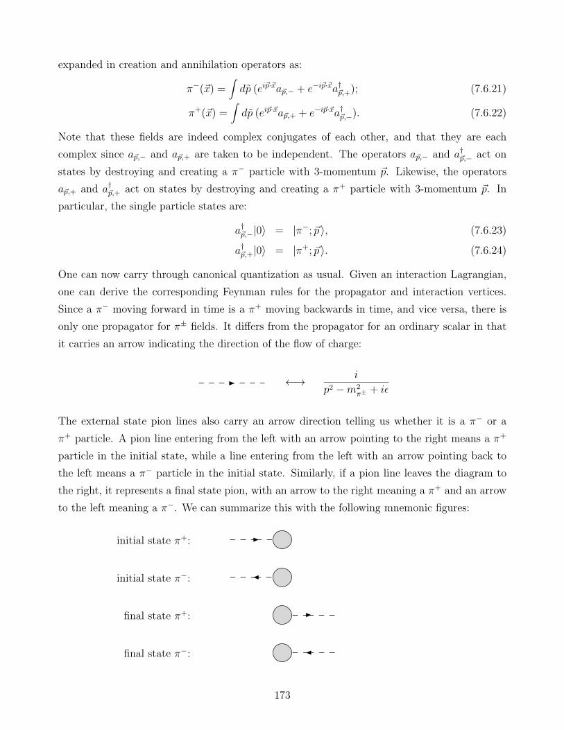
expanded in creation and annihilation operators as:

π−(~x) =∫dp (ei~p·~xa~p,− + e−i~p·~xa†~p,+); (7.6.21)

π+(~x) =∫dp (ei~p·~xa~p,+ + e−i~p·~xa†~p,−). (7.6.22)

Note that these fields are indeed complex conjugates of each other, and that they are each

complex since a~p,− and a~p,+ are taken to be independent. The operators a~p,− and a†~p,− act on

states by destroying and creating a π− particle with 3-momentum ~p. Likewise, the operators

a~p,+ and a†~p,+ act on states by destroying and creating a π+ particle with 3-momentum ~p. In

particular, the single particle states are:

a†~p,−|0〉 = |π−; ~p 〉, (7.6.23)

a†~p,+|0〉 = |π+; ~p 〉. (7.6.24)

One can now carry through canonical quantization as usual. Given an interaction Lagrangian,

one can derive the corresponding Feynman rules for the propagator and interaction vertices.

Since a π− moving forward in time is a π+ moving backwards in time, and vice versa, there is

only one propagator for π± fields. It differs from the propagator for an ordinary scalar in that

it carries an arrow indicating the direction of the flow of charge:

←→ i

p2 −m2π± + iǫ

The external state pion lines also carry an arrow direction telling us whether it is a π− or a

π+ particle. A pion line entering from the left with an arrow pointing to the right means a π+

particle in the initial state, while a line entering from the left with an arrow pointing back to

the left means a π− particle in the initial state. Similarly, if a pion line leaves the diagram to

the right, it represents a final state pion, with an arrow to the right meaning a π+ and an arrow

to the left meaning a π−. We can summarize this with the following mnemonic figures:

initial state π+:

initial state π−:

final state π+:

final state π−:

173

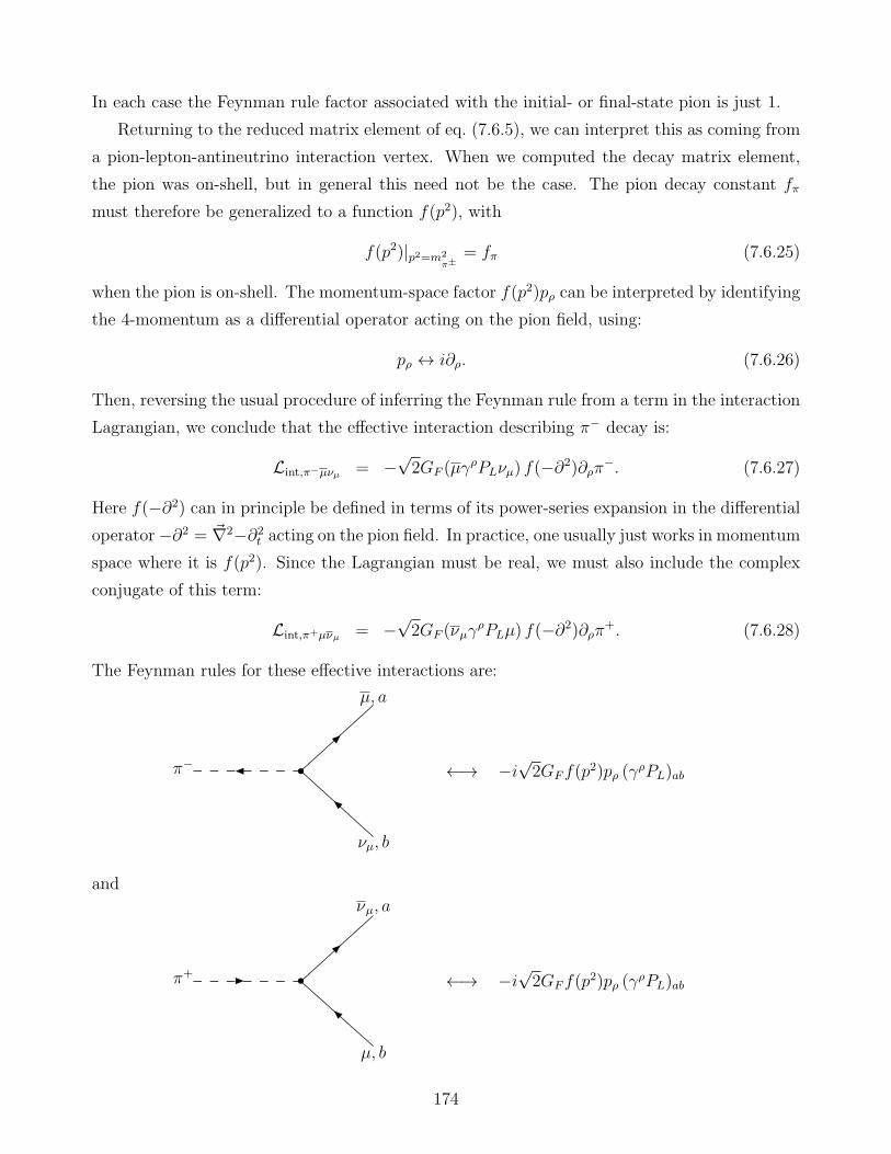
In each case the Feynman rule factor associated with the initial- or final-state pion is just 1.

Returning to the reduced matrix element of eq. (7.6.5), we can interpret this as coming from

a pion-lepton-antineutrino interaction vertex. When we computed the decay matrix element,

the pion was on-shell, but in general this need not be the case. The pion decay constant fπ

must therefore be generalized to a function f(p2), with

f(p2)|p2=m2

π±= fπ (7.6.25)

when the pion is on-shell. The momentum-space factor f(p2)pρ can be interpreted by identifying

the 4-momentum as a differential operator acting on the pion field, using:

pρ ↔ i∂ρ. (7.6.26)

Then, reversing the usual procedure of inferring the Feynman rule from a term in the interaction

Lagrangian, we conclude that the effective interaction describing π− decay is:

Lint,π−µνµ = −√2GF (µγ

ρPLνµ) f(−∂2)∂ρπ−. (7.6.27)

Here f(−∂2) can in principle be defined in terms of its power-series expansion in the differential

operator−∂2 = ~∇2−∂2t acting on the pion field. In practice, one usually just works in momentum

space where it is f(p2). Since the Lagrangian must be real, we must also include the complex

conjugate of this term:

Lint,π+µνµ = −√2GF (νµγ

ρPLµ) f(−∂2)∂ρπ+. (7.6.28)

The Feynman rules for these effective interactions are:

µ, a

νµ, b

π− ←→ −i√2GFf(p

2)pρ (γρPL)ab

and

νµ, a

µ, b

π+ ←→ −i√2GFf(p

2)pρ (γρPL)ab

174

In each Feynman diagram, the arrow on the pion line describes the direction of flow of charge,

and the 4-momentum pρ is taken to be flowing in to the vertex. When the pion is on-shell, one

can replace f(p2) by the pion decay constant fπ.

Other charged mesons made out of a quark and antiquark, like the K±, D±, and D±s , have

their own decay constants fK , fD, and fDs, and their decays can be treated in a similar way.

7.7 Unitarity, renormalizability, and the W boson

An important feature of weak-interaction 2 → 2 cross-sections following from Fermi’s four-

fermion interaction is that they grow proportional to s for very large s; see eqs. (7.4.10) and

(7.5.8). This had to be true on general grounds just from dimensional analysis. Any reduced

matrix element that contains one four-fermion interaction will be proportional to GF , so the

cross-section will have to be proportional to G2F . Since this has units of [mass]−4, and cross-

sections must have dimensions of [mass]−2, it must be that the cross-section scales like the

square of the characteristic energy of the process, s, in the high-energy limit in which all other

kinematic mass scales are comparatively unimportant. This behavior of σ ∝ s is not acceptable

for arbitrarily large s, since the cross-section is bounded by the fact that the probability for any

two particles to scatter cannot exceed 1. In quantum mechanical language, the constraint is on

the unitarity of the time-evolution operator e−iHt. If the cross-section grows too large, then our

perturbative approximation e−iHt = 1− iHt represented by the lowest-order Feynman diagram

must break down. The reduced matrix element found from just including this Feynman diagram

will have to be compensated somehow by higher-order diagrams, or by changing the physics of

the weak interactions at some higher energy scale.

Let us develop the dimensional analysis of fields and couplings further. We know that the

Lagrangian must have the same units as energy. In the standard system in which c = h = 1,

this is equal to units of [mass]. Since d3~x has units of [length]3, or [mass]−3, and

L =∫d3~x L, (7.7.1)

it must be that L has units of [mass]4. This fact allows us to evaluate the units of all fields and

couplings in a theory. For example, a spacetime derivative has units of inverse length, or [mass].

Therefore, from the kinetic terms for scalars, fermions, and vector fields found for example in

eqs. (4.1.18), (4.1.26), and (4.1.34), we find that these types of fields must have dimensions of

[mass], [mass]3/2, and [mass] respectively. This allows us to evaluate the units of various possible

interaction couplings that appear in the Lagrangian density. For example, a coupling of n scalar

fields,

Lint = −λnn!φn (7.7.2)

175

implies that λn has units of [mass]4−n. A vector-fermion-fermion coupling, like e in QED, is

dimensionless. The effective coupling fπ for on-shell pions has dimensions of [mass], because of

the presence of a spacetime derivative together with a scalar field and two fermion fields in the

Lagrangian. Summarizing this information for the known types of fields and couplings that we

have encountered so far:

Object Dimension Role

L [mass]4 Lagrangian density

∂µ [mass] derivative

φ [mass] scalar field

Ψ [mass]3/2 fermion field

Aµ [mass] vector field

λ3 [mass] scalar3 coupling

λ4 [mass]0 scalar4 coupling

y [mass]0 scalar-fermion-fermion (Yukawa) coupling

e [mass]0 photon-fermion-fermion coupling

GF [mass]−2 fermion4 coupling

fπ [mass] fermion2-scalar-derivative coupling

u, v, u, v [mass]1/2 external-state spinors

MNi→Nf[mass]4−Ni−Nf reduced matrix element for Ni → Nf particles

σ [mass]−2 cross-section

Γ [mass] decay rate.

(7.7.3)

It is a general fact that theories with couplings with negative mass dimension, like GF , or λn

for n ≥ 5, always suffer from a problem known as non-renormalizability.† In a renormalizable

theory, the divergences that occur in loop diagrams due to integrating over arbitrarily large

4-momenta for virtual particles can be regularized by introducing a high momentum cutoff, and

then the resulting dependence on the unknown cutoff can be absorbed into a redefinition of the

masses and coupling constants of the theory. In contrast, in a non-renormalizable theory, one

finds that this process requires introducing an infinite number of different couplings, each of

which must be redefined in order to absorb the momentum-cutoff dependence. This dependence

on an infinite number of different coupling constants makes non-renormalizable theories non-

predictive, although only in principle. We can always use non-renormalizable theories as effective

theories at low energies, as we have done in the case of the four-fermion theory of the weak

†The converse is not true; just because a theory has only couplings with positive or zero mass dimension doesnot guarantee that it is renormalizable. It is a necessary, but not sufficient, condition.

176

interactions. However, when probed at sufficiently high energies, a non-renormalizable theory

will encounter related problems associated with the apparent failure of unitarity (cross-sections

that grow uncontrollably with energy) and non-renormalizability (an uncontrollable dependence

on more and more unknown couplings that become more and more important at higher energies).

For this reason, we are happier to describe physical phenomena using renormalizable theories if

we can.

An example of a useful non-renormalizable theory is gravity. The effective coupling constant

for Feynman diagrams involving gravitons is 1/M2Planck, where MPlanck = 2.4 × 1018 GeV is

the “reduced Planck mass”. Like GF , this coupling has negative mass dimension, so tree-level

cross-sections for 2 → 2 scattering involving gravitons grow with energy like s. This is not a

problem as long as we stick to scattering energies ≪ MPlanck, which corresponds to all known

experiments and directly measured phenomena. However, we do not know how unitarity is

restored in gravitational interactions at energies comparable to MPlanck or higher. Unlike the

case of the weak interactions, it is hard to conceive of an experiment with present technologies

that could test competing ideas.

To find a renormalizable “fix” for the weak interactions, we note that the (V − A)(V − A)current-current structure of the four-fermion coupling could come about from the exchange of

a heavy vector particle. To do this, we imagine “pulling apart” the two currents, and replacing

the short line segment by the propagator for a virtual vector particle. For example, one of the

current-current terms is:

µ, a e, c

νµ, b νe, d

←→

µ, a e, c

νµ, b νe, d

W

Since the currents involved have electric charges −1 and +1, the vector boson must carry charge

−1 to the right. This is the W− vector boson. By analogy with the charged pion, W± are

complex vector fields, with an arrow on its propagator indicating the direction of flow of charge.

The Feynman rule for the propagator of a charged vector W± boson carrying 4-momentum

p turns out to be:

←→ i

p2 −m2W + iǫ

[−gρσ +

pρpσm2

W

]ρ σ

177

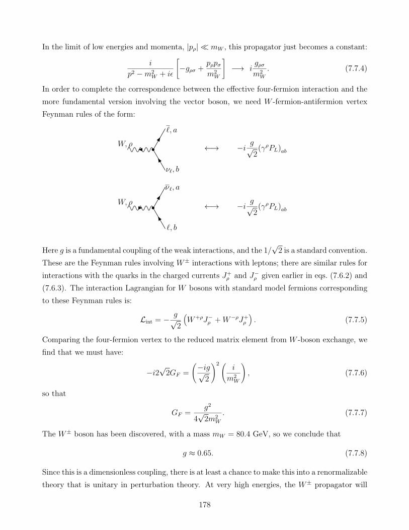
In the limit of low energies and momenta, |pρ| ≪ mW , this propagator just becomes a constant:

i

p2 −m2W + iǫ

[−gρσ +

pρpσm2

W

]−→ i

gρσm2

W

. (7.7.4)

In order to complete the correspondence between the effective four-fermion interaction and the

more fundamental version involving the vector boson, we need W -fermion-antifermion vertex

Feynman rules of the form:

←→ −i g√2(γρPL)ab

νℓ, b

ℓ, a

W, ρ

←→ −i g√2(γρPL)ab

ℓ, b

νℓ, a

W, ρ

Here g is a fundamental coupling of the weak interactions, and the 1/√2 is a standard convention.

These are the Feynman rules involving W± interactions with leptons; there are similar rules for

interactions with the quarks in the charged currents J+ρ and J−

ρ given earlier in eqs. (7.6.2) and

(7.6.3). The interaction Lagrangian for W bosons with standard model fermions corresponding

to these Feynman rules is:

Lint = −g√2

(W+ρJ−

ρ +W−ρJ+ρ

). (7.7.5)

Comparing the four-fermion vertex to the reduced matrix element from W -boson exchange, we

find that we must have:

−i2√2GF =

(−ig√2

)2 (i

m2W

), (7.7.6)

so that

GF =g2

4√2m2

W

. (7.7.7)

The W± boson has been discovered, with a mass mW = 80.4 GeV, so we conclude that

g ≈ 0.65. (7.7.8)

Since this is a dimensionless coupling, there is at least a chance to make this into a renormalizable

theory that is unitary in perturbation theory. At very high energies, the W± propagator will

178

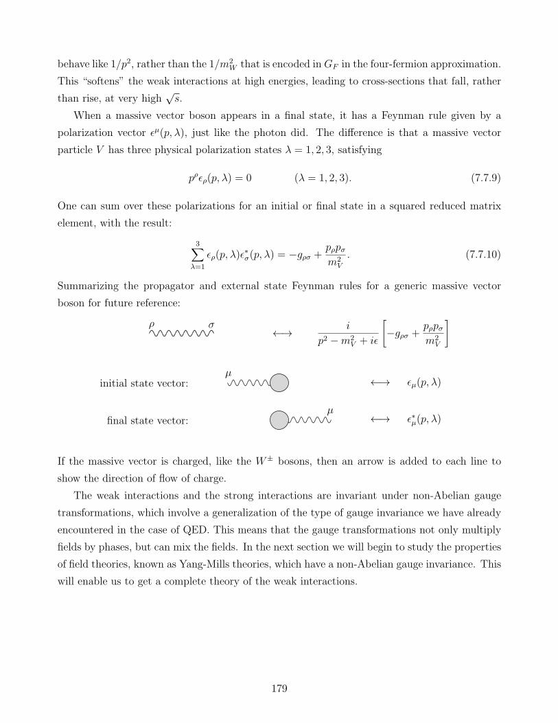
behave like 1/p2, rather than the 1/m2W that is encoded in GF in the four-fermion approximation.

This “softens” the weak interactions at high energies, leading to cross-sections that fall, rather

than rise, at very high√s.

When a massive vector boson appears in a final state, it has a Feynman rule given by a

polarization vector ǫµ(p, λ), just like the photon did. The difference is that a massive vector

particle V has three physical polarization states λ = 1, 2, 3, satisfying

pρǫρ(p, λ) = 0 (λ = 1, 2, 3). (7.7.9)

One can sum over these polarizations for an initial or final state in a squared reduced matrix

element, with the result:

3∑

λ=1

ǫρ(p, λ)ǫ∗σ(p, λ) = −gρσ +

pρpσm2

V

. (7.7.10)

Summarizing the propagator and external state Feynman rules for a generic massive vector

boson for future reference:

←→ i

p2 −m2V + iǫ

[−gρσ +

pρpσm2

V

]ρ σ

µ←→ ǫµ(p, λ)initial state vector:

µfinal state vector: ←→ ǫ∗µ(p, λ)

If the massive vector is charged, like the W± bosons, then an arrow is added to each line to

show the direction of flow of charge.

The weak interactions and the strong interactions are invariant under non-Abelian gauge

transformations, which involve a generalization of the type of gauge invariance we have already

encountered in the case of QED. This means that the gauge transformations not only multiply

fields by phases, but can mix the fields. In the next section we will begin to study the properties

of field theories, known as Yang-Mills theories, which have a non-Abelian gauge invariance. This

will enable us to get a complete theory of the weak interactions.

179

8 Gauge theories

8.1 Groups and representations

In this section, we will generalize the idea of gauge invariance found in electrodynamics. Recall

that in QED the Lagrangian is defined in terms of a covariant derivative

Dµ = ∂µ + iQeAµ (8.1.1)

and a field strength

Fµν = ∂µAν − ∂νAµ (8.1.2)

as

L = −1

4F µνFµν + iΨ /DΨ−mΨΨ. (8.1.3)

This Lagrangian is invariant under the local gauge transformation

Aµ → A′µ = Aµ −

1

e∂µθ, (8.1.4)

Ψ → Ψ′ = eiQθΨ, (8.1.5)

where θ(x) is any function of spacetime, called a gauge parameter. Now, the result of doing one

gauge transformation θ1 followed by another gauge transformation θ2 is always a third gauge

transformation parameterized by the function θ1 + θ2:

Aµ → (Aµ −1

e∂µθ1)−

1

e∂µθ2 = Aµ −

1

e∂µ(θ1 + θ2), (8.1.6)

Ψ→ eiQθ2(eiQθ1Ψ) = eiQ(θ1+θ2)Ψ. (8.1.7)

Mathematically, these gauge transformations are an example of a group.

A group is a set of elements G = gi and a rule for multiplying them, with the properties:

1) Closure: If gi and gj are elements of the group G, then the product gigj is also an element

of G.

2) Associativity: gi(gjgk) = (gigj)gk.

3) Existence of an Identity: There is a unique element I = g1 of the group, such that for all

gi in G, Igi = giI = gi.

4) Inversion: For each gi, there is a unique inverse element (gi)−1 satisfying (gi)

−1gi =

gi(gi)−1 = I.

180

It may or may not be also true that the group also satisfies the commutativity property:

gigj = gjgi. (8.1.8)

If this is satisfied, then the group is called commutative or Abelian. Otherwise it is non-

commutative or non-Abelian.

In generalizing the QED Lagrangian, we will be interested in continuous Lie groups. A

continuous group has an uncountably infinite number of elements labeled by one or more con-

tinuously varying parameters, which turn out to be nothing other than the generalizations of

the gauge parameter θ in QED. A Lie group is a continuous group that also has the desirable

property of being differentiable with respect to the gauge parameters.

The action of group elements on physics states or fields can be represented by a set of complex

n × n matrices acting on n-dimensional complex vectors. This association of group elements

with n× n matrices and the states or fields that they act on is said to form a representation of

the group. The matrices obey the same rules as the group elements themselves.

For example, the group of QED gauge transformations is the Abelian Lie group U(1). Ac-

cording to eq. (8.1.5), the group is represented on Dirac fermion fields by complex 1×1 matrices:

UQ(θ) = eiQθ. (8.1.9)

Here θ labels the group elements, and the charge Q labels the representation of the group. So

we can say that the electron, muon, and tau Dirac fields each live in a representation of the

group U(1) with charge Q = −1; the Dirac fields for up, charm, and top quarks each live in a

representation with charge Q = 2/3; and the Dirac fields for down, strange and bottom quarks

each live in a representation with Q = −1/3. We can read off the charge of any field if we know

how it transforms under the gauge group. A barred Dirac field transforms with the opposite

phase from the original Dirac field of charge Q, and therefore has charge −Q.Objects that transform into themselves with no change are said to be in the singlet rep-

resentation. In general, the Lagrangian should be invariant under gauge transformations, and

therefore must be in the singlet representation. For example, each term of the QED Lagrangian

carries no charge, and so is a singlet of U(1). The photon field Aµ has charge 0, and is therefore

usually said (by a slight abuse of language) to transform as a singlet representation of U(1).

[Technically, it does not really transform under gauge transformations as any representation of

the group U(1), because of the derivative term in eq. (8.1.4), unless θ is a constant function so

that one is making the same transformation everywhere in spacetime.]

Let us now generalize to non-Abelian groups, which always involve representations contain-

ing more than one field or state. Let ϕi be a set of objects that together transform in some

181

representation R of the group G. The number of components of ϕi is called the dimension of

the representation, dR, so that i = 1, . . . , dR. Under a group transformation,

ϕi → ϕ′i = Ui

jϕj (8.1.10)

where Uij is a representation matrix. We are especially interested in transformations that are

represented by unitary matrices, so that their action can be realized on the quantum Hilbert

space by a unitary operator. Consider the subset of group elements that are infinitesimally close

to the identity element. We can write these in the form:

U(ǫ)ij = (1 + iǫaT a)i

j. (8.1.11)

Here the T aji are a basis for all the possible infinitesimal group transformations. The number

of matrices T a is called the dimension of the group, dG, and there is an implicit sum over

a = 1, . . . , dG. The ǫa are a set of dG infinitesimal gauge parameters (analogous to θ in QED)

that tell us how much of each is included in the transformation represented by U(ǫ). Since U(ǫ)

is unitary,

U(ǫ)† = U(ǫ)−1 = 1− iǫaT a, (8.1.12)

from which it follows that the matrices T a must be Hermitian.

Consider two group transformations gǫ and gδ parameterized by ǫa and δa. By the closure

property we can then form a new group element

gǫgδg−1ǫ g−1

δ . (8.1.13)

Working with some particular representation, this corresponds to

U(ǫ)U(δ)U(ǫ)−1U(δ)−1 = (1 + iǫaT a)(1 + iδbT b)(1− iǫcT c)(1− iδdT d) (8.1.14)

= 1− ǫaδb[T a, T b] + . . . (8.1.15)

The closure property requires that this is a representation of the group element in eq. (8.1.13),

which must also be close to the identity. It follows that

[T a, T b] = ifabcT c (8.1.16)

for some set of numbers fabc, called the structure constants of the group. In practice, one often

picks a particular representation of matrices T a as the defining or fundamental representation.

This determines the structure constants fabc once and for all. The set of matrices T a for

all other representations are then required to reproduce eq. (8.1.16), which fixes their overall

182

normalization. Equation (8.1.16) defines the Lie algebra corresponding to the Lie group, and

the hermitian matrices T a are said to be generators of the Lie algebra for the corresponding

representation. Many physicists have a bad habit of using the words “Lie group” and “Lie

algebra” interchangeably, because we often only care about the subset of gauge transformations

that are close to the identity.

For any given representation R, one can always choose the generators so that:

Tr(T aRT

bR) = I(R)δab. (8.1.17)

The number I(R) is called the index of the representation. A standard choice is that the index

of the fundamental representation of a non-Abelian Lie algebra is 1/2. (This can always be

achieved by rescaling the T a, if necessary.) From eqs. (8.1.16) and (8.1.17), one obtains for any

representation R:

iI(R)fabc = Tr([T aR, T

bR]T

cR). (8.1.18)

It follows, from the cyclic property of the trace, that fabc is totally antisymmetric under inter-

change of any two of a, b, c. By using the Jacobi identity,

[T a, [T b, T c]] + [T b, [T c, T a]] + [T c, [T a, T b]] = 0, (8.1.19)

which holds for any three matrices, one also finds the useful result:

fadef bce + f cdefabe + f bdef cae = 0. (8.1.20)

Two representations R and R′ are said to be equivalent if there exists some fixed matrix X

such that:

XT aRX

−1 = T aR′ , (8.1.21)

for all a. Obviously, this requires that R and R′ have the same dimension. From a physical

point of view, equivalent representations are indistinguishable from each other.

A representation R of a Lie algebra is said to be reducible if it is equivalent to a representation

in block-diagonal form; in other words, if there is some matrix X that can be used to put all of

the T aR simultaneously in a block-diagonal form:

XT aRX

−1 =

T ar1

0 . . . 00 T a

r2. . . 0

......

. . ....

0 0 . . . T arn

for all a. (8.1.22)

183

Here the T ariare representation matrices for smaller representations ri. One calls this a direct

sum, and writes it as

R = r1 ⊕ r2 ⊕ . . .⊕ rn. (8.1.23)

A representation that is not equivalent to a direct sum of smaller representations in this way is

said to be irreducible. Heuristically, reducible representations are those that can be chopped up

into smaller pieces that can be consistently treated individually.

With the above conventions on the Lie algebra generators, one can show that for each

irreducible representation R:

(T aRT

aR)i

j = C(R)δji (8.1.24)

(with an implicit sum over a = 1, . . . , dG), where C(R) is another characteristic number of the

representation R, called the quadratic Casimir invariant. If we take the sum over a of eq. (8.1.17),

it is equal to the trace of eq. (8.1.24). It follows that for each irreducible representation R, the

dimension, the index, and the Casimir invariant are related to the dimension of the group by:

dGI(R) = dRC(R). (8.1.25)

The simplest irreducible representation of any Lie algebra is just:

T aji = 0. (8.1.26)

This is called the singlet representation.

Suppose that we have some representation with matrices T aji . Then one can show that

the matrices −(T aji )∗ also form a representation of the algebra eq. (8.1.16). This is called the

complex conjugate of the representation R, and is often denoted R:

T aR= −T a∗

R . (8.1.27)

If T aRis equivalent to T a

R, so that there is some fixed matrix X such that

XT aRX−1 = T a

R, (8.1.28)

then the representation R is said to be a real representation,† and otherwise R is said to be

complex.

†Real representations can be divided into two sub-cases, “positive-real” and “pseudo-real”, depending onwhether the matrix X can or cannot be chosen to be symmetric. In a pseudo-real representation, the T a cannotall be made antisymmetric and imaginary; in a positive-real representation, they can.

184

One can also form the tensor product of any two representations R, R′ of the Lie algebra to

get another representation:

(T aR⊗R′)i,x

j,y ≡ (T aR)i

jδyx + δji (TaR′)x

y. (8.1.29)

The representation R⊗R′ has dimension dRdR′ , and is typically reducible:

R⊗R′ = R1 ⊕ . . .⊕Rn (8.1.30)

with

dR⊗R′ = dRdR′ = dR1+ . . .+ dRn

. (8.1.31)

This is a way to make larger representations (R1 . . . Rn out of smaller ones (R,R′).

One can check from the identity eq. (8.1.20) that the matrices

(T a)bc = −ifabc (8.1.32)

form a representation, called the adjoint representation, with the same dimension as the group

G. As a matter of terminology, the quadratic Casimir invariant of the adjoint representation

is also called the Casimir invariant of the group, and given the symbol C(G). Note that, from

eq. (8.1.25), the index of the adjoint representation is equal to its quadratic Casimir invariant:

C(G) ≡ C(adjoint) = I(adjoint). (8.1.33)

We now list, without proof, some further group theory facts regarding Lie algebra represen-

tations:

• The number of inequivalent irreducible representations of a Lie group is always infinite.

• Unlike group element multiplication, the tensor product multiplication of representations

is both associative and commutative:

(R1 ⊗R2)⊗R3 = R1 ⊗ (R2 ⊗R3), (8.1.34)

R1 ⊗R2 = R2 ⊗R1. (8.1.35)

• The tensor product of any representation with the singlet representation just gives the

original representation back:

1⊗R = R⊗ 1 = R. (8.1.36)

• The tensor product of two real representations R1 and R2 is always a direct sum of repre-

sentations that are either real or appear in complex conjugate pairs.

185

• The adjoint representation is always real.

• The tensor product of two irreducible representations contains the singlet representation

if and only if they are complex conjugates of each other:

R1 ⊗R2 = 1⊕ . . . ←→ R2 = R1. (8.1.37)

It follows that if R is real, then R⊗R contains a singlet.

• The tensor product of a representation and its complex conjugate always contains both

the singlet and adjoint representations:

R⊗R = 1⊕ Adjoint⊕ . . . . (8.1.38)

• As a corollary of the preceding rules, the tensor product of the adjoint representation with

itself always contains both the singlet and the adjoint:

Adjoint⊗ Adjoint = 1S ⊕ AdjointA ⊕ . . . . (8.1.39)

Here the S and A mean that the indices of the two adjoints on the left are combined

symmetrically and antisymmetrically respectively.

• If the tensor product of two representations contains a third, then the tensor product of the

first representation with the conjugate of the third representation contains the conjugate

of the second representation:

R1 ⊗R2 = R3 ⊕ . . . , ←→ R1 ⊗R3 = R2 ⊕ . . . , (8.1.40)

R1 ⊗R2 ⊗R3 = 1⊕ . . . , ←→ R1 ⊗R2 = R3 ⊕ . . . . (8.1.41)

• If R1 ⊗R2 = r1 ⊕ . . .⊕ rn, then the indices satisfy the following rule:

I(R1)dR2+ I(R2)dR1

=n∑

i=1

I(ri). (8.1.42)

Let us recall how Lie algebra representations work in the example of SU(2), the group of

unitary 2× 2 matrices (that’s the “U(2)” part of the name) with determinant 1 (that’s the “S”,

for special, part of the name). This group is familiar from the study of angular momentum in

quantum mechanics, and the defining or fundamental representation is the familiar spin-1/2 one

with ϕi with i = 1, 2 or up,down. The Lie algebra generators in the fundamental representation

are:

T a =σa

2(a = 1, 2, 3), (8.1.43)

186

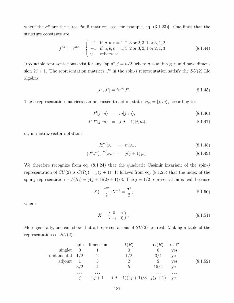
where the σa are the three Pauli matrices [see, for example, eq. (3.1.23)]. One finds that the

structure constants are

fabc = ǫabc =

+1 if a, b, c = 1, 2, 3 or 2, 3, 1 or 3, 1, 2−1 if a, b, c = 1, 3, 2 or 3, 2, 1 or 2, 1, 30 otherwise.

(8.1.44)

Irreducible representations exist for any “spin” j = n/2, where n is an integer, and have dimen-

sion 2j + 1. The representation matrices Ja in the spin-j representation satisfy the SU(2) Lie

algebra:

[Ja, J b] = iǫabcJ c. (8.1.45)

These representation matrices can be chosen to act on states ϕm = |j,m〉, according to:

J3|j,m〉 = m|j,m〉, (8.1.46)

JaJa|j,m〉 = j(j + 1)|j,m〉, (8.1.47)

or, in matrix-vector notation:

J3m′

m ϕm′ = mϕm, (8.1.48)

(JaJa)mm′

ϕm′ = j(j + 1)ϕm. (8.1.49)

We therefore recognize from eq. (8.1.24) that the quadratic Casimir invariant of the spin-j

representation of SU(2) is C(Rj) = j(j + 1). It follows from eq. (8.1.25) that the index of the

spin-j representation is I(Rj) = j(j + 1)(2j + 1)/3. The j = 1/2 representation is real, because

X(−σa∗

2)X−1 =

σa

2, (8.1.50)

where

X =(

0 i−i 0

). (8.1.51)

More generally, one can show that all representations of SU(2) are real. Making a table of the

representations of SU(2):

spin dimension I(R) C(R) real?singlet 0 1 0 0 yes

fundamental 1/2 2 1/2 3/4 yesadjoint 1 3 2 2 yes

3/2 4 5 15/4 yes. . . . . . . . . . . . . . .j 2j + 1 j(j + 1)(2j + 1)/3 j(j + 1) yes

(8.1.52)

187

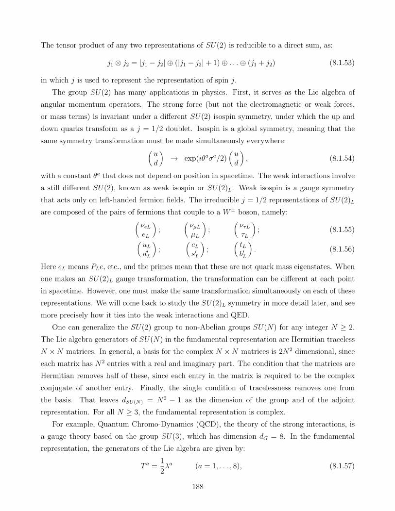
The tensor product of any two representations of SU(2) is reducible to a direct sum, as:

j1 ⊗ j2 = |j1 − j2| ⊕ (|j1 − j2|+ 1)⊕ . . .⊕ (j1 + j2) (8.1.53)

in which j is used to represent the representation of spin j.

The group SU(2) has many applications in physics. First, it serves as the Lie algebra of

angular momentum operators. The strong force (but not the electromagnetic or weak forces,

or mass terms) is invariant under a different SU(2) isospin symmetry, under which the up and

down quarks transform as a j = 1/2 doublet. Isospin is a global symmetry, meaning that the

same symmetry transformation must be made simultaneously everywhere:(ud

)→ exp(iθaσa/2)

(ud

), (8.1.54)

with a constant θa that does not depend on position in spacetime. The weak interactions involve

a still different SU(2), known as weak isospin or SU(2)L. Weak isospin is a gauge symmetry

that acts only on left-handed fermion fields. The irreducible j = 1/2 representations of SU(2)L

are composed of the pairs of fermions that couple to a W± boson, namely:(νeLeL

);

(νµLµL

);

(ντLτL

); (8.1.55)

(uLd′L

);

(cLs′L

);

(tLb′L

). (8.1.56)

Here eL means PLe, etc., and the primes mean that these are not quark mass eigenstates. When

one makes an SU(2)L gauge transformation, the transformation can be different at each point

in spacetime. However, one must make the same transformation simultaneously on each of these

representations. We will come back to study the SU(2)L symmetry in more detail later, and see

more precisely how it ties into the weak interactions and QED.

One can generalize the SU(2) group to non-Abelian groups SU(N) for any integer N ≥ 2.

The Lie algebra generators of SU(N) in the fundamental representation are Hermitian traceless

N ×N matrices. In general, a basis for the complex N ×N matrices is 2N2 dimensional, since

each matrix has N2 entries with a real and imaginary part. The condition that the matrices are

Hermitian removes half of these, since each entry in the matrix is required to be the complex

conjugate of another entry. Finally, the single condition of tracelessness removes one from

the basis. That leaves dSU(N) = N2 − 1 as the dimension of the group and of the adjoint

representation. For all N ≥ 3, the fundamental representation is complex.

For example, Quantum Chromo-Dynamics (QCD), the theory of the strong interactions, is

a gauge theory based on the group SU(3), which has dimension dG = 8. In the fundamental

representation, the generators of the Lie algebra are given by:

T a =1

2λa (a = 1, . . . , 8), (8.1.57)

188

where the λa are known as the Gell-Mann matrices:

λ1 =

0 1 01 0 00 0 0

; λ2 =

0 −i 0i 0 00 0 0

; λ3 =

1 0 00 −1 00 0 0

;

λ4 =

0 0 10 0 01 0 0

; λ5 =

0 0 −i0 0 0i 0 0

; λ6 =

0 0 00 0 10 1 0

;

λ7 =

0 0 00 0 −i0 i 0

; λ8 =

1√3

1 0 00 1 00 0 −2

. (8.1.58)

Note that each of these matrices is Hermitian and traceless, as required. They have also been

engineered to satisfy Tr(λaλb) = 2δab, so that

Tr(T aT b) =1

2δab, (8.1.59)

and therefore the index of the fundamental representation is

I(F ) = 1/2. (8.1.60)

One can also check that

(T aT a)ij =

4

3δji , (8.1.61)

so that the quadratic Casimir invariant of the fundamental representation is

C(F ) = 4/3. (8.1.62)

By taking commutators of each pair of generators, one finds that the non-zero structure constants

of SU(3) are:

f 123 = 1; (8.1.63)

f 147 = −f 156 = f 246 = f 257 = f 345 = −f 367 = 1/2; (8.1.64)

f 458 = f 678 =√3/2. (8.1.65)

and those related to the above by permutations of indices, following from the condition that

the fabc are totally antisymmetric. From these one can find the adjoint representation matrices

using eq. (8.1.32), with, for example:

T 1adjoint = −i

0 0 0 0 0 0 0 00 0 1 0 0 0 0 00 −1 0 0 0 0 0 00 0 0 0 0 0 1/2 00 0 0 0 0 −1/2 0 00 0 0 0 1/2 0 0 00 0 0 −1/2 0 0 0 00 0 0 0 0 0 0 0

, (8.1.66)

189

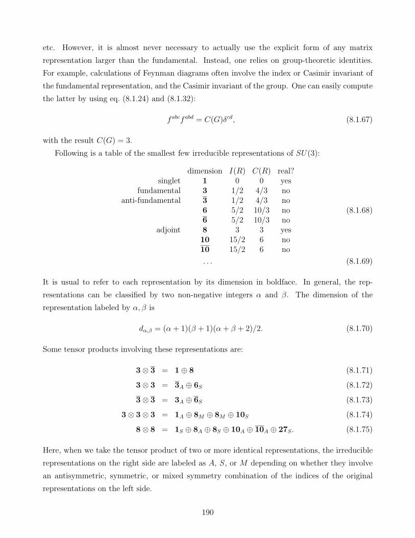
etc. However, it is almost never necessary to actually use the explicit form of any matrix

representation larger than the fundamental. Instead, one relies on group-theoretic identities.

For example, calculations of Feynman diagrams often involve the index or Casimir invariant of

the fundamental representation, and the Casimir invariant of the group. One can easily compute

the latter by using eq. (8.1.24) and (8.1.32):

fabcfabd = C(G)δcd, (8.1.67)

with the result C(G) = 3.

Following is a table of the smallest few irreducible representations of SU(3):

dimension I(R) C(R) real?singlet 1 0 0 yes

fundamental 3 1/2 4/3 noanti-fundamental 3 1/2 4/3 no

6 5/2 10/3 no6 5/2 10/3 no

adjoint 8 3 3 yes10 15/2 6 no10 15/2 6 no

(8.1.68)

. . . (8.1.69)

It is usual to refer to each representation by its dimension in boldface. In general, the rep-

resentations can be classified by two non-negative integers α and β. The dimension of the

representation labeled by α, β is

dα,β = (α + 1)(β + 1)(α + β + 2)/2. (8.1.70)

Some tensor products involving these representations are:

3⊗ 3 = 1⊕ 8 (8.1.71)

3⊗ 3 = 3A ⊕ 6S (8.1.72)

3⊗ 3 = 3A ⊕ 6S (8.1.73)

3⊗ 3⊗ 3 = 1A ⊕ 8M ⊕ 8M ⊕ 10S (8.1.74)

8⊗ 8 = 1S ⊕ 8A ⊕ 8S ⊕ 10A ⊕ 10A ⊕ 27S. (8.1.75)

Here, when we take the tensor product of two or more identical representations, the irreducible

representations on the right side are labeled as A, S, or M depending on whether they involve

an antisymmetric, symmetric, or mixed symmetry combination of the indices of the original

representations on the left side.

190

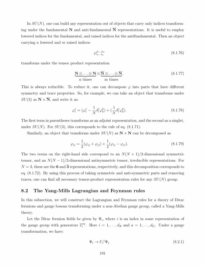
In SU(N), one can build any representation out of objects that carry only indices transform-

ing under the fundamental N and anti-fundamental N representations. It is useful to employ

lowered indices for the fundamental, and raised indices for the antifundamental. Then an object

carrying n lowered and m raised indices:

ϕj1...jmi1...in (8.1.76)

transforms under the tensor product representation

N⊗ . . .⊗N︸ ︷︷ ︸n times

⊗N⊗ . . .⊗N︸ ︷︷ ︸m times

. (8.1.77)

This is always reducible. To reduce it, one can decompose ϕ into parts that have different

symmetry and trace properties. So, for example, we can take an object that transforms under

SU(3) as N×N, and write it as:

ϕji = (ϕj

i −1

Nδjiϕ

kk) + (

1

Nδjiϕ

kk). (8.1.78)

The first term in parentheses transforms as an adjoint representation, and the second as a singlet,

under SU(N). For SU(3), this corresponds to the rule of eq. (8.1.71).

Similarly, an object that transforms under SU(N) as N×N can be decomposed as

ϕij =1

2(ϕij + ϕji) +

1

2(ϕij − ϕji). (8.1.79)

The two terms on the right-hand side correspond to an N(N + 1)/2-dimensional symmetric

tensor, and an N(N − 1)/2-dimensional antisymmetric tensor, irreducible representations. For

N = 3, these are the 6 and 3 representations, respectively, and this decomposition corresponds to

eq. (8.1.72). By using this process of taking symmetric and anti-symmetric parts and removing

traces, one can find all necessary tensor-product representation rules for any SU(N) group.

8.2 The Yang-Mills Lagrangian and Feynman rules

In this subsection, we will construct the Lagrangian and Feynman rules for a theory of Dirac

fermions and gauge bosons transforming under a non-Abelian gauge group, called a Yang-Mills

theory.

Let the Dirac fermion fields be given by Ψi, where i is an index in some representation of

the gauge group with generators T aji . Here i = 1, . . . , dR and a = 1, . . . , dG. Under a gauge

transformation, we have:

Ψi → UijΨj (8.2.1)

191

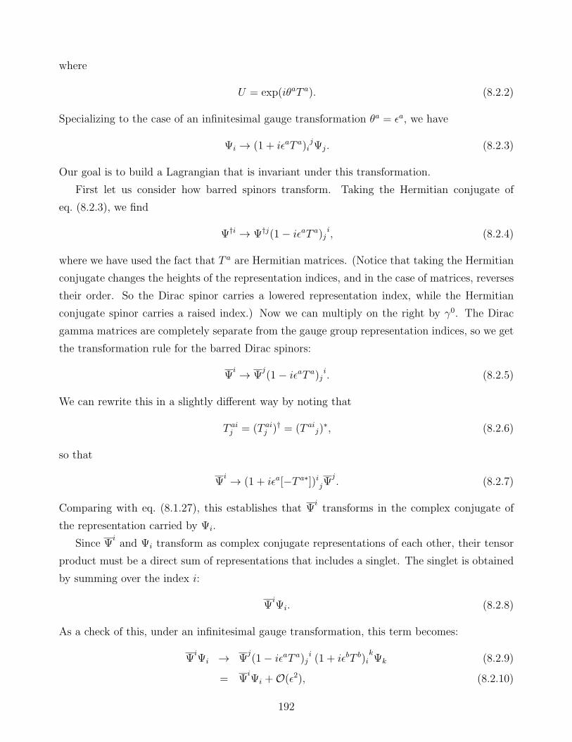
where

U = exp(iθaT a). (8.2.2)

Specializing to the case of an infinitesimal gauge transformation θa = ǫa, we have

Ψi → (1 + iǫaT a)ijΨj. (8.2.3)

Our goal is to build a Lagrangian that is invariant under this transformation.

First let us consider how barred spinors transform. Taking the Hermitian conjugate of

eq. (8.2.3), we find

Ψ†i → Ψ†j(1− iǫaT a)ji, (8.2.4)

where we have used the fact that T a are Hermitian matrices. (Notice that taking the Hermitian

conjugate changes the heights of the representation indices, and in the case of matrices, reverses

their order. So the Dirac spinor carries a lowered representation index, while the Hermitian

conjugate spinor carries a raised index.) Now we can multiply on the right by γ0. The Dirac

gamma matrices are completely separate from the gauge group representation indices, so we get

the transformation rule for the barred Dirac spinors:

Ψi → Ψ

j(1− iǫaT a)j

i. (8.2.5)

We can rewrite this in a slightly different way by noting that

T aij = (T ai

j )† = (T aij)

∗, (8.2.6)

so that

Ψi → (1 + iǫa[−T a∗])ijΨ

j. (8.2.7)

Comparing with eq. (8.1.27), this establishes that Ψitransforms in the complex conjugate of

the representation carried by Ψi.

Since Ψiand Ψi transform as complex conjugate representations of each other, their tensor

product must be a direct sum of representations that includes a singlet. The singlet is obtained

by summing over the index i:

ΨiΨi. (8.2.8)

As a check of this, under an infinitesimal gauge transformation, this term becomes:

ΨiΨi → Ψ

j(1− iǫaT a)j

i (1 + iǫbT b)ikΨk (8.2.9)

= ΨiΨi +O(ǫ2), (8.2.10)

192

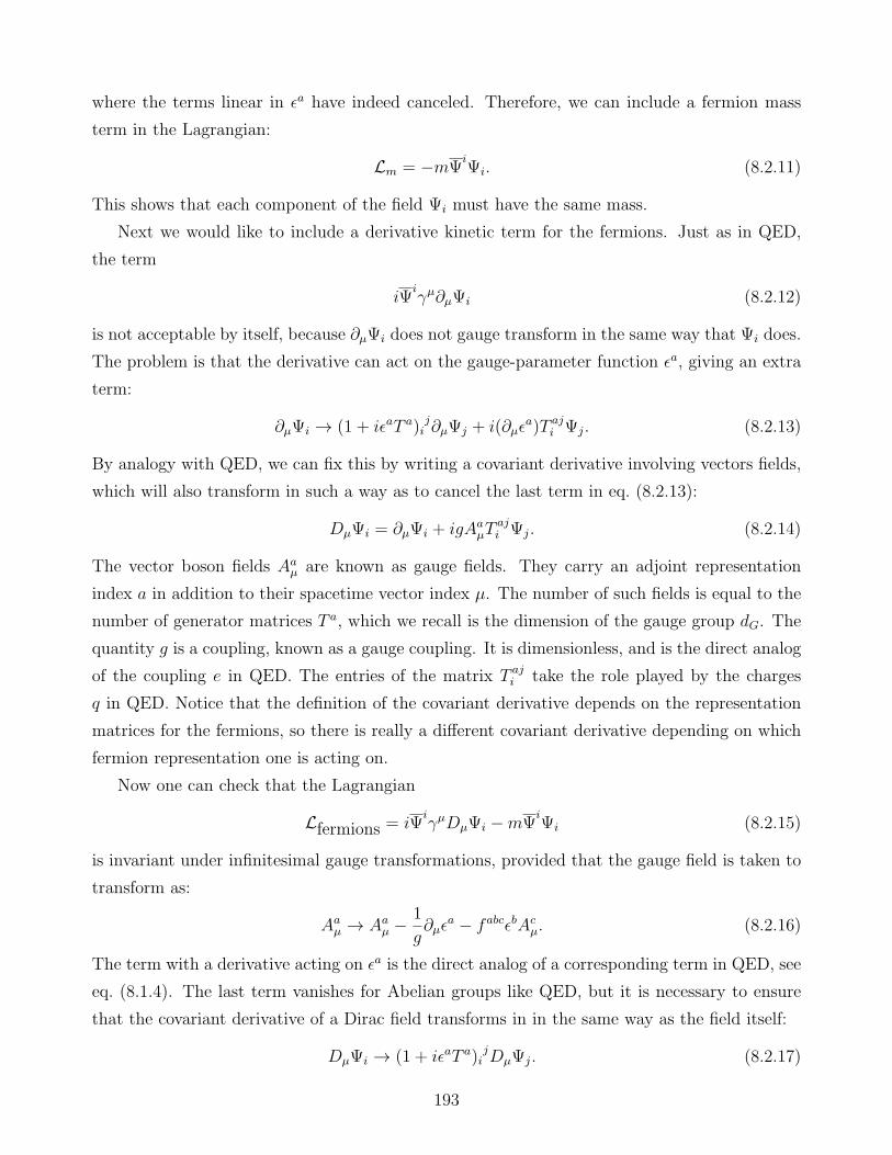
where the terms linear in ǫa have indeed canceled. Therefore, we can include a fermion mass

term in the Lagrangian:

Lm = −mΨiΨi. (8.2.11)

This shows that each component of the field Ψi must have the same mass.

Next we would like to include a derivative kinetic term for the fermions. Just as in QED,

the term

iΨiγµ∂µΨi (8.2.12)

is not acceptable by itself, because ∂µΨi does not gauge transform in the same way that Ψi does.

The problem is that the derivative can act on the gauge-parameter function ǫa, giving an extra

term:

∂µΨi → (1 + iǫaT a)ij∂µΨj + i(∂µǫ

a)T aji Ψj. (8.2.13)

By analogy with QED, we can fix this by writing a covariant derivative involving vectors fields,

which will also transform in such a way as to cancel the last term in eq. (8.2.13):

DµΨi = ∂µΨi + igAaµT

aji Ψj. (8.2.14)

The vector boson fields Aaµ are known as gauge fields. They carry an adjoint representation

index a in addition to their spacetime vector index µ. The number of such fields is equal to the

number of generator matrices T a, which we recall is the dimension of the gauge group dG. The

quantity g is a coupling, known as a gauge coupling. It is dimensionless, and is the direct analog

of the coupling e in QED. The entries of the matrix T aji take the role played by the charges

q in QED. Notice that the definition of the covariant derivative depends on the representation

matrices for the fermions, so there is really a different covariant derivative depending on which

fermion representation one is acting on.

Now one can check that the Lagrangian

Lfermions = iΨiγµDµΨi −mΨ

iΨi (8.2.15)

is invariant under infinitesimal gauge transformations, provided that the gauge field is taken to

transform as:

Aaµ → Aa

µ −1

g∂µǫ

a − fabcǫbAcµ. (8.2.16)

The term with a derivative acting on ǫa is the direct analog of a corresponding term in QED, see

eq. (8.1.4). The last term vanishes for Abelian groups like QED, but it is necessary to ensure

that the covariant derivative of a Dirac field transforms in in the same way as the field itself:

DµΨi → (1 + iǫaT a)ijDµΨj. (8.2.17)

193

If we limit ourselves to constant gauge parameters ∂µǫa = 0, then the transformation in

eq. (8.2.16) is of the correct form for a field in the adjoint representation.

Having introduced a gauge field for each Lie algebra generator, we must now include kinetic

terms for them. By analogy with QED, the gauge field Lagrangian has the form:

Lgauge = −1

4F µνaF a

µν , (8.2.18)

with an implied sum on a, where F aµν is an antisymmetric field strength tensor for each Lie

algebra generator. However, we must also require that this Lagrangian is invariant under gauge

transformations. This is accomplished if we choose:

F aµν = ∂µA

aν − ∂νAa

µ − gfabcAbµA

cν . (8.2.19)

Then one can check, using eq. (8.2.16), that

F aµν → F a

µν − fabcǫbF cµν . (8.2.20)

From this it follows that Lgauge transforms as:

−1

4F µνaF a

µν → −1

4F µνaF a

µν −1

2F µνafabcǫbF c

µν +O(ǫ2). (8.2.21)

The extra term linear in ǫ vanishes, because the part F µνaF cµν is symmetric under interchange

of a↔ c, but its gauge indices are contracted with fabc, which is antisymmetric under the same

interchange. Therefore, eq. (8.2.18) is a gauge singlet.

Putting the above results together, we have found a gauge-invariant Lagrangian for Dirac

fermions coupled to a non-Abelian gauge field:

LYang−Mills = Lgauge + Lfermions. (8.2.22)

Now we can find the Feynman rules for this theory in the usual way. First we identify the

kinetic terms that are quadratic in the fields. That part of LYang-Mills is:

Lkinetic = −1

4(∂µA

aν − ∂νAa

µ)(∂µAaν − ∂νAaµ) + iΨ

i/∂Ψi −mΨiΨi. (8.2.23)

These terms have exactly the same form as in the QED Lagrangian, but with a sum over dG

copies of the vector fields, labeled by a, and over dR copies of the fermion field, labeled by i.

Therefore we can obtain the Feynman rules for vector and fermion propagators in the same

way. For the gauge fields, we need to include a gauge-fixing term, just as in QED [compare

eq. (5.1.32) and the surrounding discussion], in order to have a well-defined propagator:

Lgauge−fixing = − 1

2ξ(∂µAa

µ)2 (8.2.24)

with the index a summed over. This leads to:

194

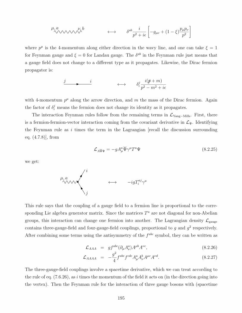
←→ δabi

p2 + iǫ

[−gµν + (1− ξ)pµpν

p2

]µ, a ν, b

where pµ is the 4-momentum along either direction in the wavy line, and one can take ξ = 1

for Feynman gauge and ξ = 0 for Landau gauge. The δab in the Feynman rule just means that

a gauge field does not change to a different type as it propagates. Likewise, the Dirac fermion

propagator is:

←→ δjii(/p+m)

p2 −m2 + iǫ

j i

with 4-momentum pµ along the arrow direction, and m the mass of the Dirac fermion. Again

the factor of δji means the fermion does not change its identity as it propagates.

The interaction Feynman rules follow from the remaining terms in LYang−Mills. First, there

is a fermion-fermion-vector interaction coming from the covariant derivative in LΨ. Identifying

the Feynman rule as i times the term in the Lagrangian [recall the discussion surrounding

eq. (4.7.8)], from

LAΨΨ = −gAaµΨγ

µT aΨ (8.2.25)

we get:

←→ −igT aji γµ

j

i

µ, a

This rule says that the coupling of a gauge field to a fermion line is proportional to the corre-

sponding Lie algebra generator matrix. Since the matrices T a are not diagonal for non-Abelian

groups, this interaction can change one fermion into another. The Lagrangian density Lgauge

contains three-gauge-field and four-gauge-field couplings, proportional to g and g2 respectively.

After combining some terms using the antisymmetry of the fabc symbol, they can be written as

LAAA = gfabc(∂µAaν)A

µbAνc, (8.2.26)

LAAAA = −g2

4fabef cdeAa

µAbνA

µcAνd. (8.2.27)

The three-gauge-field couplings involve a spacetime derivative, which we can treat according to

the rule of eq. (7.6.26), as i times the momentum of the field it acts on (in the direction going into

the vertex). Then the Feynman rule for the interaction of three gauge bosons with (spacetime

195

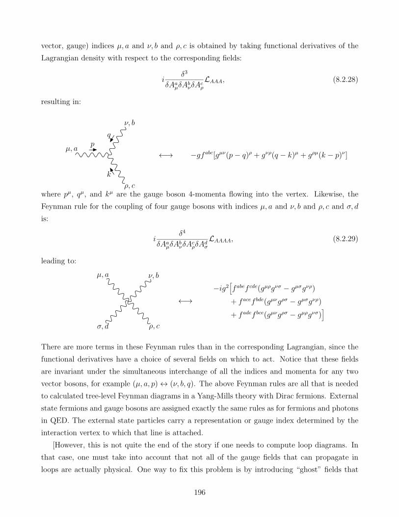
vector, gauge) indices µ, a and ν, b and ρ, c is obtained by taking functional derivatives of the

Lagrangian density with respect to the corresponding fields:

iδ3

δAaµδA

bνδA

cρ

LAAA, (8.2.28)

resulting in:

←→ −gfabc[gµν(p− q)ρ + gνρ(q − k)µ + gρµ(k − p)ν ]

ρ, c

ν, b

µ, ap

q

k

where pµ, qµ, and kµ are the gauge boson 4-momenta flowing into the vertex. Likewise, the

Feynman rule for the coupling of four gauge bosons with indices µ, a and ν, b and ρ, c and σ, d

is:

iδ4

δAaµδA

bνδA

cρδA

dσ

LAAAA, (8.2.29)

leading to:

←→−ig2

[fabef cde(gµρgνσ − gµσgνρ)+ facef bde(gµνgρσ − gµσgνρ)+ fadef bce(gµνgρσ − gµρgνσ)

]

µ, a ν, b

ρ, cσ, d

There are more terms in these Feynman rules than in the corresponding Lagrangian, since the

functional derivatives have a choice of several fields on which to act. Notice that these fields

are invariant under the simultaneous interchange of all the indices and momenta for any two

vector bosons, for example (µ, a, p)↔ (ν, b, q). The above Feynman rules are all that is needed

to calculated tree-level Feynman diagrams in a Yang-Mills theory with Dirac fermions. External

state fermions and gauge bosons are assigned exactly the same rules as for fermions and photons

in QED. The external state particles carry a representation or gauge index determined by the

interaction vertex to which that line is attached.

[However, this is not quite the end of the story if one needs to compute loop diagrams. In

that case, one must take into account that not all of the gauge fields that can propagate in

loops are actually physical. One way to fix this problem is by introducing “ghost” fields that

196

only appear in loops, never in initial or final states. The ghost fields do not create and destroy

real particles; they are really just book-keeping devices that exist only to cancel the unphysical

contributions of gauge fields in loops. We will not do any loop calculations in this course, so we

will not go into more detail on that issue.]

The Yang-Mills theory we have constructed makes several interesting predictions. One is

that the gauge fields are necessarily massless. If one tries to get around this by introducing a

mass term for the vector gauge fields, like:

LA−mass = m2VA

aµA

aµ, (8.2.30)

then one finds that this term is not invariant under the gauge transformation of eq. (8.2.16).

Therefore, if we put in such a term, we necessarily violate the gauge invariance of the Lagrangian,

and the gauge symmetry will not be a symmetry of the theory. This sounds like a serious

problem, because there is only one known freely-propagating, non-composite, massless vector

field, the photon. In particular, the massive W± boson cannot be described by the Yang-Mills

theory that we have so far. One way to proceed would be to simply keep the term in eq. (8.2.30),

and accept that the theory is not fully invariant under the gauge symmetry. The only problem

with this is that the theory would be non-renormalizable in that case; as a related problem,

unitarity would be violated in scattering at very high energies. Instead, we can explain the

non-zero mass of the W± boson by enlarging the theory to include scalar fields, leading to a

spontaneous breakdown in the gauge symmetry.

Another nice feature of the Yang-Mills theory is that several different couplings are predicted

to be related to each other. Once we have picked a gauge group G, a set of irreducible represen-

tations for the fermions, and the gauge coupling g, then the interaction terms are all fixed. In

particular, if we know the coupling of one type of fermion to the gauge fields, then we know g.

This in turn allows us to predict, as a consequence of the gauge invariance, what the couplings

of other fermions to the gauge fields should be (as long as we know their representations), and

what the three-gauge-boson and four-gauge-boson vertices should be.

197

9 Quantum Chromo-Dynamics (QCD)

9.1 QCD Lagrangian and Feynman rules

The strong interactions are based on a Yang-Mills theory with gauge group SU(3)c, with quarks

transforming in the fundamental 3 representation. The subscript c is to distinguish this as the

group of invariances under transformations of the color degrees of freedom. As far as we can

tell, this is an exact symmetry of nature. (There is also an approximate SU(3)flavor symmetry

under which the quark flavors u, d, s transform into each other; isospin is an SU(2) subgroup

of this symmetry.) Each of the quark Dirac fields u, d, s, c, b, t transforms separately as a 3

of SU(3)c, and each barred Dirac field u, d, s, c, b, t therefore transforms as a 3, as we saw on

general grounds in subsection 8.2.

For example, an up quark is created in an initial state by any one of the three color component

fields:

u =

uredublueugreen

=

u1u2u3

, (9.1.1)

while an anti-up quark is created in an initial state by any of the fields:

u = ( ured ublue ugreen ) = ( u1 u2 u3 ) . (9.1.2)

Since SU(3)c is an exact symmetry, no experiment can tell the difference between a red quark

and a blue quark, so the labels are intrinsically arbitrary. In fact, we can do a different SU(3)c

transformation at each point in spacetime, but simultaneously on each quark flavor, so that:

u→ eiθa(x)Ta

u, d→ eiθa(x)Ta

d, s→ eiθa(x)Ta

s, etc., (9.1.3)

where T a = λa

2with a = 1, . . . , 8, and the θa(x) are any gauge parameter functions of our

choosing. This symmetry is in addition to the U(1)EM gauge transformations:

u→ eiθ(x)Quu, d→ eiθ(x)Qdd, s→ eiθ(x)Qss, etc., (9.1.4)

where Qu = Qc = Qt = 2/3 and Qd = Qs = Qb = −1/3. For each of the 8 generator matrices

T a of SU(3)c, there is a corresponding gauge vector boson called a gluon, represented by a field

Gaµ carrying both a spacetime vector index and an SU(3)c adjoint representation index.

One says that the unbroken gauge group of the Standard Model is SU(3)c × U(1)EM, withthe fermions and gauge bosons transforming as:

198

SU(3)c × U(1)EM spin

u, c, t (3,+23) 1

2

d, s, b (3,−13) 1

2

e, µ, τ (1,−1) 12

νe, νµ, ντ (1, 0) 12

γ (1, 0) 1

gluon (8, 0) 1

The gluon appears together with the photon field Aµ in the full covariant derivative for

quark fields. Using an index i = 1, 2, 3 to run over the color degrees of freedom, the covariant

derivatives are:

Dµui = ∂µui + ig3GaµT

aji uj + ieAµ(

2

3)ui, (9.1.5)

Dµdi = ∂µdi + ig3GaµT

aji dj + ieAµ(−

1

3)di. (9.1.6)

Here g3 is the coupling constant associated with the SU(3)c gauge interactions. The strength

of the strong interactions comes from the fact that g3 ≫ e.

Using the general results for a gauge theory in subsection 8.2, we know that the propagator

for the gluon is that of a massless vector field just like the photon:

←→ δabi

p2 + iǫ

[−gµν + (1− ξ)pµpν

p2

]µ, a ν, b

Note that it is traditional, in QCD, to use “springy” lines for gluons, to easily distinguish them

from wavy photon lines. There are also quark-gluon interaction vertices for each flavor of quark:

←→ −ig3T aji γµ

j

i

µ, a

Here the quark line can be any of u, d, s, c, b, t. The gluon interaction changes the color of the

quarks when T a is non-diagonal, but never changes the flavor of the quark line, so an up quark

remains an up quark, a down quark remains a down quark, etc.

The Lagrangian density also contains a “pure glue” part:

Lglue = −1

4F µνaF a

µν (9.1.7)

F aµν = ∂µG

aν − ∂νGa

µ − g3fabcGbµG

cν , (9.1.8)

where fabc are the structure constants for SU(3)c given in eqs. (8.1.63)-(8.1.65). In addition to

the propagator, this implies that there are three-gluon and four-gluon interactions:

199

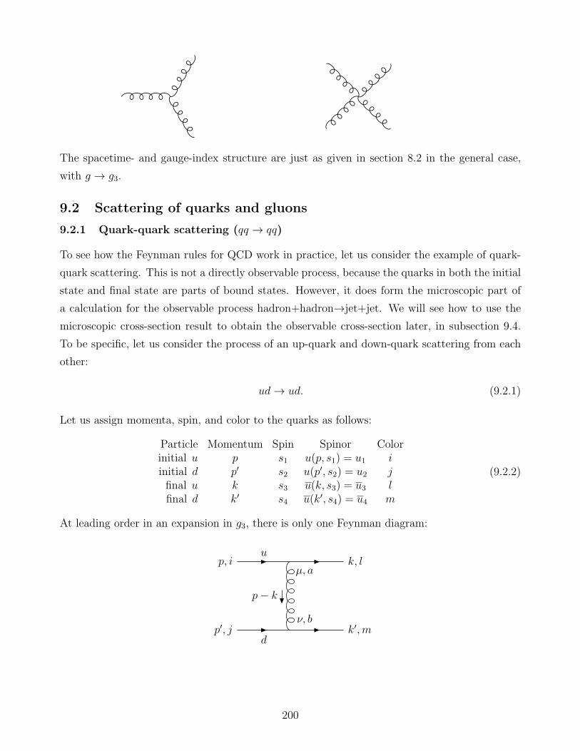
The spacetime- and gauge-index structure are just as given in section 8.2 in the general case,

with g → g3.

9.2 Scattering of quarks and gluons

9.2.1 Quark-quark scattering (qq → qq)

To see how the Feynman rules for QCD work in practice, let us consider the example of quark-

quark scattering. This is not a directly observable process, because the quarks in both the initial

state and final state are parts of bound states. However, it does form the microscopic part of

a calculation for the observable process hadron+hadron→jet+jet. We will see how to use the

microscopic cross-section result to obtain the observable cross-section later, in subsection 9.4.

To be specific, let us consider the process of an up-quark and down-quark scattering from each

other:

ud→ ud. (9.2.1)

Let us assign momenta, spin, and color to the quarks as follows:

Particle Momentum Spin Spinor Colorinitial u p s1 u(p, s1) = u1 iinitial d p′ s2 u(p′, s2) = u2 jfinal u k s3 u(k, s3) = u3 lfinal d k′ s4 u(k′, s4) = u4 m

(9.2.2)

At leading order in an expansion in g3, there is only one Feynman diagram:

u

d

p, i

p′, j

k, l

k′,m

p− k

µ, a

ν, b

200

The reduced matrix element can now be written down by the same procedure as in QED. One

obtains, using Feynman gauge (ξ = 1):

M =[u3(−ig3γµT ai

l )u1] [u4(−ig3γνT bj

m )u2] [−igµνδab

(p− k)2]

(9.2.3)

= ig23Tail T

ajm [u3γµu1] [u4γ

µu2] /t (9.2.4)

where t = (p − k)2. This matrix element is exactly what one finds in QED for e−µ− → e−µ−,

but with the QED squared coupling replaced by a product of matrices depending on the color

combination:

e2 → g23Tail T

ajm . (9.2.5)

This illustrates that the “color charge matrix” g3Tail is analogous to the electric charge eQf .

There are 34 = 81 color combinations for quark-quark scattering.

In order to find the differential cross-section, we continue as usual by taking the complex

square of the reduced matrix element:

|M|2 = g43(Tail T

ajm )(T bi

l Tbjm )∗|M|2, (9.2.6)

for each i, j, l,m (with no implied sum yet), and

M = [u3γµu1] [u4γµu2] /t. (9.2.7)

It is not possible, even in principle, to distinguish between colors. However, one can always

imagine fixing, by an arbitrary choice, that the incoming u-quark has color red= 1; then the

colors of the other quarks can be distinguished up to SU(3)c rotations that leave the red com-

ponent fixed. In practice, one does not measure the colors of quarks in an experiment, even

with respect to some arbitrary choice, so we will sum over the colors of the final state quarks

and average over the colors of the initial state quarks:

1

3

∑

i

1

3

∑

j

∑

l

∑

m

|M|2. (9.2.8)

To do the color sum/average most easily, we note that, because the gauge group generator

matrices are Hermitian,

(T bil T

bjm )∗ = (T bl

i Tbmj ). (9.2.9)

Therefore, the color factor is

1

3

∑

i

1

3

∑

j

∑

l

∑

m

(T ail T

ajm )(T bi

l Tbjm )∗ =

1

9

∑

i,j,l,m

(T ail T

bli )(T

ajm T bm

j ) (9.2.10)

201

=1

9Tr(T aT b)Tr(T aT b) (9.2.11)

=1

9I(3)δabI(3)δab (9.2.12)

=1

9(1

2)2dG (9.2.13)

=2

9(9.2.14)

In doing this, we have used the definition of the index of a representation eq. (8.1.17); the fact

that the index of the fundamental representation is 1/2; and the fact that the sum over a, b of

δabδab just counts the number of generators of the Lie algebra dG, which is 8 for SU(3)c.

Meanwhile, the rest of |M|2, including a sum over final state spins and an average over initial

state spins, can be taken directly from the corresponding result for e−µ− → e−µ− in QED, which

we found by crossing symmetry in eq. (5.3.23). Stripping off the factor e4 associated with the

QED charges, we find in the high energy limit of negligible quark masses,

1

2

∑

s1

1

2

∑

s2

∑

s3

∑

s4

|M|2 = 2

(s2 + u2

t2

). (9.2.15)

Putting this together with the factor of g43 and the color factor above, we have

|M|2 ≡ 1

9

∑

colors

1

4

∑

spins

|M|2 = 4g439

(s2 + u2

t2

). (9.2.16)

The notation |M|2 is a standard notation, which for a general process implies the appropriate

sum/average over spin and color. The differential cross-section for this process is therefore:

dσ

d(cos θ)=

1

32πs|M|2 = 2πα2

s

9s

(s2 + u2

t2

), (9.2.17)

where

αs =g234π

(9.2.18)

is the strong-interaction analog of the fine structure constant. Since we are neglecting quark

masses, the kinematics for this process is the same as in any massless 2→2 process, for example

as found in eqs. (5.2.139)-(5.2.143). Therefore, one can replace cos θ in favor of the Mandelstam

variable t, using

d(cos θ) =2dt

s, (9.2.19)

so

dσ

dt=

4πα2s

9s2

(s2 + u2

t2

). (9.2.20)

202

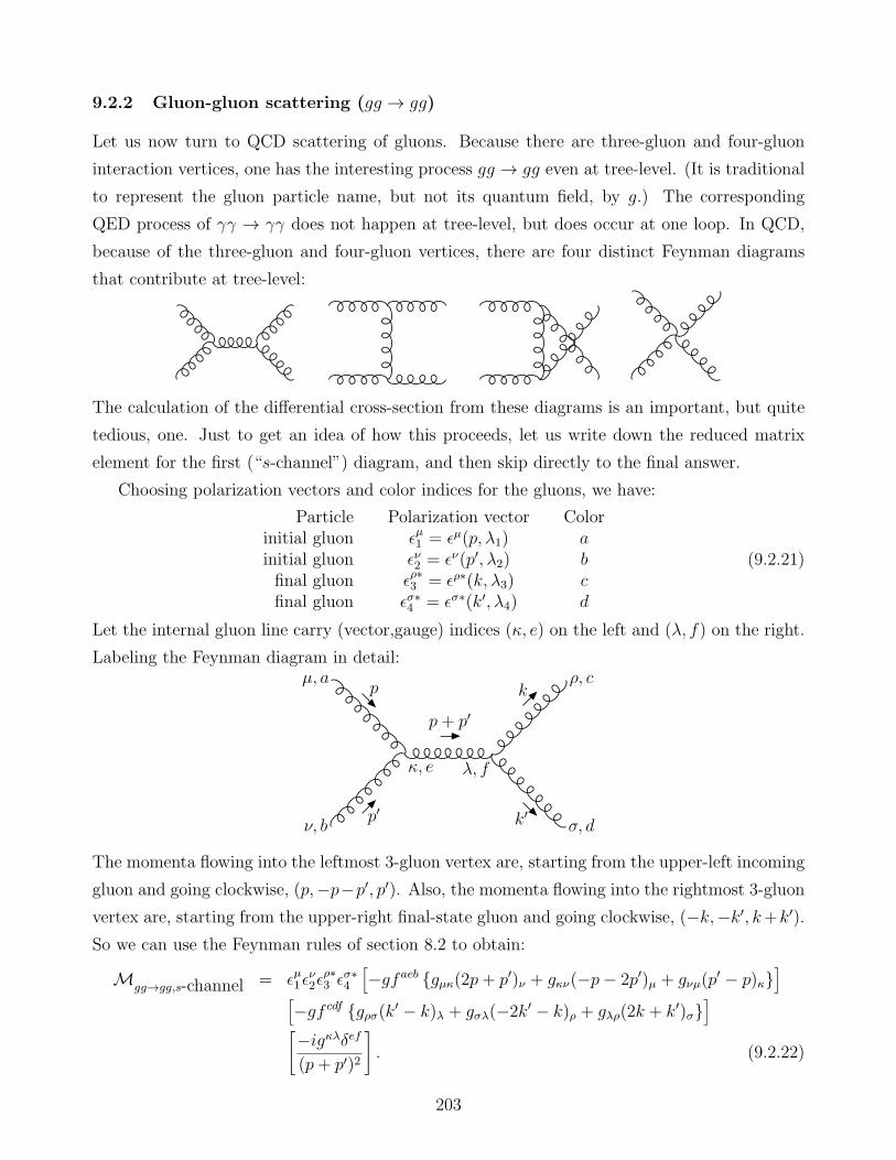
9.2.2 Gluon-gluon scattering (gg → gg)

Let us now turn to QCD scattering of gluons. Because there are three-gluon and four-gluon

interaction vertices, one has the interesting process gg → gg even at tree-level. (It is traditional

to represent the gluon particle name, but not its quantum field, by g.) The corresponding

QED process of γγ → γγ does not happen at tree-level, but does occur at one loop. In QCD,

because of the three-gluon and four-gluon vertices, there are four distinct Feynman diagrams

that contribute at tree-level:

The calculation of the differential cross-section from these diagrams is an important, but quite

tedious, one. Just to get an idea of how this proceeds, let us write down the reduced matrix

element for the first (“s-channel”) diagram, and then skip directly to the final answer.

Choosing polarization vectors and color indices for the gluons, we have:

Particle Polarization vector Colorinitial gluon ǫµ1 = ǫµ(p, λ1) ainitial gluon ǫν2 = ǫν(p′, λ2) bfinal gluon ǫρ∗3 = ǫρ∗(k, λ3) cfinal gluon ǫσ∗4 = ǫσ∗(k′, λ4) d

(9.2.21)

Let the internal gluon line carry (vector,gauge) indices (κ, e) on the left and (λ, f) on the right.

Labeling the Feynman diagram in detail:

p+ p′

p

p′

k

k′

µ, a

ν, b

ρ, c

σ, d

κ, e λ, f

The momenta flowing into the leftmost 3-gluon vertex are, starting from the upper-left incoming

gluon and going clockwise, (p,−p−p′, p′). Also, the momenta flowing into the rightmost 3-gluon

vertex are, starting from the upper-right final-state gluon and going clockwise, (−k,−k′, k+k′).So we can use the Feynman rules of section 8.2 to obtain:

Mgg→gg,s-channel = ǫµ1ǫ

ν2ǫ

ρ∗3 ǫ

σ∗4

[−gfaeb gµκ(2p+ p′)ν + gκν(−p− 2p′)µ + gνµ(p

′ − p)κ]

[−gf cdf gρσ(k′ − k)λ + gσλ(−2k′ − k)ρ + gλρ(2k + k′)σ

]

[−igκλδef(p+ p′)2

]. (9.2.22)

203

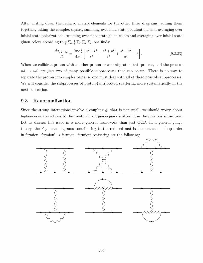
After writing down the reduced matrix elements for the other three diagrams, adding them

together, taking the complex square, summing over final state polarizations and averaging over

initial state polarizations, summing over final-state gluon colors and averaging over initial-state

gluon colors according to 18

∑a

18

∑b

∑c

∑d one finds:

dσgg→gg

dt=

9πα2s

4s2

[u2 + t2

s2+s2 + u2

t2+s2 + t2

u2+ 3

]. (9.2.23)

When we collide a proton with another proton or an antiproton, this process, and the process

ud → ud, are just two of many possible subprocesses that can occur. There is no way to

separate the proton into simpler parts, so one must deal with all of these possible subprocesses.

We will consider the subprocesses of proton-(anti)proton scattering more systematically in the

next subsection.

9.3 Renormalization

Since the strong interactions involve a coupling g3 that is not small, we should worry about

higher-order corrections to the treatment of quark-quark scattering in the previous subsection.

Let us discuss this issue in a more general framework than just QCD. In a general gauge

theory, the Feynman diagrams contributing to the reduced matrix element at one-loop order

in fermion+fermion′ → fermion+fermion′ scattering are the following:

204

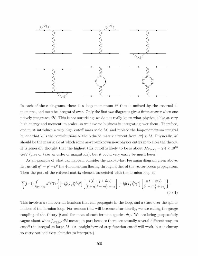
In each of these diagrams, there is a loop momentum ℓµ that is unfixed by the external 4-

momenta, and must be integrated over. Only the first two diagrams give a finite answer when one

naively integrates d4ℓ. This is not surprising; we do not really know what physics is like at very

high energy and momentum scales, so we have no business in integrating over them. Therefore,

one must introduce a very high cutoff mass scale M , and replace the loop-momentum integral

by one that kills the contributions to the reduced matrix element from |ℓµ| ≥M . Physically, M

should be the mass scale at which some as-yet-unknown new physics enters in to alter the theory.

It is generally thought that the highest this cutoff is likely to be is about MPlanck = 2.4 × 1018

GeV (give or take an order of magnitude), but it could very easily be much lower.

As an example of what can happen, consider the next-to-last Feynman diagram given above.

Let us call qµ = pµ−kµ the 4-momentum flowing through either of the vector-boson propagators.

Then the part of the reduced matrix element associated with the fermion loop is:

∑

f

(−1)∫

|ℓµ|≤Md4ℓ Tr

[−ig(Tf )aji γµ

] [ i(/ℓ + /q + mf )

(ℓ+ q)2 − m2f + iǫ

] [−ig(Tf )bij γν

] [ i(/ℓ + mf )

ℓ2 − m2f + iǫ

].

(9.3.1)

This involves a sum over all fermions that can propagate in the loop, and a trace over the spinor

indices of the fermion loop. For reasons that will become clear shortly, we are calling the gauge

coupling of the theory g and the mass of each fermion species mf . We are being purposefully

vague about what∫|ℓµ|≤M d4ℓ means, in part because there are actually several different ways to

cutoff the integral at large M . (A straightforward step-function cutoff will work, but is clumsy

to carry out and even clumsier to interpret.)

205

The d4ℓ factor can be written as an angular part times a radial part |ℓ|3d|ℓ|. Now there are

up to five powers of |ℓ| in the numerator (three from the d4ℓ, and two from the propagators),

and four powers of |ℓ| in the denominator from the propagators. So naively, one might expect

that the result of doing the integral will scale like M2 for a large cutoff M . However, there is

a conspiratorial cancellation, so that the large-M behavior is only logarithmic. The result is

proportional to:

g2(q2gµν − qµqν)∑

f

Tr(T af T

bf ) [ln (M/m) + . . .] (9.3.2)

where the . . . represents a contribution that does not get large as M gets large. The m is a

characteristic mass scale of the problem; it is something with dimensions of mass built out of qµ

and the mf . It must appear in the formula in the way it does in order to make the argument of

the logarithm dimensionless. The arbitrariness in the precise definition of m can be absorbed

into the “. . .”.

When one uses eq. (9.3.2) in the rest of the Feynman diagram, it is clear that the entire

contribution must be proportional to:

Mfermion loop in gauge propagator ∝ g4∑

f

I(Rf )ln(M/m) + . . . . (9.3.3)

What we are trying to keep track of here is just the number of powers of g, the group-theory

factor, and the large-M dependence on ln(M/m).

A similar sort of calculation applies to the last diagram involving a gauge vector boson loop.

Each of the three-vector couplings involves a factor of fabc, with two of the indices contracted

because of the propagators. So it must be that the loop part of the diagram make a contribution

proportional to facdf bcd = C(G)δab. It is again logarithmically divergent, so that

Mgauge loop in gauge propagator ∝ g4C(G)ln(M/m) + . . . . (9.3.4)

Doing everything carefully, one finds that the contributions to the differential cross-section is

given by:

dσ = dσtree(g)

1 +

g2

4π2

113C(G)− 4

3

∑

f

I(Rf )

ln(M/m) + . . .

, (9.3.5)

where dσtree(g) is the tree-level result (which we have already worked out in the special case of

QCD), considered to be a function of g. To be specific, it is proportional to g4. Let us ignore

all the other diagrams for now; the justification for this will be revealed soon.

The cutoffM may be quite large. Furthermore, we typically do not know what it is, or what

the specific very-high-energy physics associated with it is. (If we did, we could just redo the

206

calculation with that physics included, and a higher cutoff.) Therefore, it is convenient to absorb

our ignorance of M into a redefinition of the coupling. Specifically, inspired by eq. (9.3.5), one

defines a renormalized or running coupling g(µ) by writing:

g = g(µ)

1−

(g(µ))2

16π2

113C(G)− 4

3

∑

f

I(Rf )

ln(M/µ)

, (9.3.6)

Here µ is a new mass scale, called the renormalization scale, that we get to pick. (It is not

uncommon to see the renormalization scale denoted by Q instead of µ.) The original coupling

g is called the bare coupling. One can invert this relation to write the renormalized coupling in

terms of the bare coupling:

g(µ) = g

1 +

g2

16π2

113C(G)− 4

3

∑

f

I(Rf )

ln(M/µ) + . . .

, (9.3.7)

where we are treating g(µ) as an expansion in g, dropping terms of order g5 everywhere.

The reason for this strategic definition is that, since we know that dσtree(g) is proportional

to g4, we can now write, using eqs. (9.3.5) and (9.3.6):

dσ = dσtree(g) (g/g)4

1 +

g2

4π2

113C(G)− 4

3

∑

f

I(Rf )

ln(M/m) + . . .

(9.3.8)

= dσtree(g)

1 +

g2

4π2

113C(G)− 4

3

∑

f

I(Rf )

ln(µ/m) + . . .

. (9.3.9)

Here we are again dropping terms that go like g4; these are comparable to 2-loop contributions

that we are neglecting anyway. The factor dσtree(g) is the tree-level differential cross-section,

but with g(µ) in place of g. This formula looks very much like eq. (9.3.5), but with the crucial

difference that the unknown cutoff M has disappeared, and is replaced by the scale µ that we

know, because we get to pick it.

What should we pick µ to be? In principle we could pick it to be the cutoff M , except that

we do not know what that is. Besides, the logarithm could then be very large, and perturbation

theory would converge very slowly or not at all. For example, suppose that M = MPlanck,

and the characteristic energy scale of the experiment we are doing is, say, m = 0.511 MeV or

m = 1000 GeV. These choice might be appropriate for experiments involving a non-relativistic

electron and a TeV-scale collider, respectively. Then

ln(M/m) ≈ 50 or 35. (9.3.10)

This logarithm typically gets multiplied by 1/16π2 times g2 times a group-theory quantity, but

is still large. This suggests that a really good choice for µ is to make the logarithm ln(µ/m)

207

as small as possible, so that the correction term in eq. (9.3.9) is small. Therefore, one should

choose

µ ≈ m. (9.3.11)

Then, to a first approximation, one can calculate using the tree-level approximation using a

renormalized coupling g(µ), knowing that the one-loop correction from these diagrams is small.

The choice of renormalization scale eq. (9.3.11) allows us to write:

dσ ≈ dσtree(g(µ)). (9.3.12)

Of course, this is only good enough to get rid of the large logarithmic one-loop corrections. If

you really want all one-loop corrections, there is no way around calculating all the one-loop

diagrams, keeping all the pieces, not just the ones that get large as M →∞.

What about the remaining diagrams? If we isolate the M → ∞ behavior, they fall into

three classes. First, there are diagrams that are not divergent at all (the first two diagram).

Second, there are diagrams (the third through sixth diagrams) that are individually divergent

like ln(M/m), but sum up to a total that is not divergent. Finally, the seventh through tenth

diagrams have a logarithmic divergence, but it can be absorbed into a similar redefinition of the

mass. A clue to this is that they all involve sub-diagrams:

The one-loop renormalized or running mass mf (µ) is defined in terms of the bare mass mf by

mf = mf (µ)

(1− g2

2π2C(Rf )ln(M/µ)

), (9.3.13)

or

mf (µ) = mf

(1 +

g2

2π2C(Rf )ln(M/µ) + . . .

), (9.3.14)

where C(Rf ) is the quadratic Casimir invariant of the representation carried by the fermion f .

It is an amazing fact that the two redefinitions eqs. (9.3.6) and (9.3.13) are enough to remove

the cutoff dependence of all cross-sections in the theory up to and including one-loop order. In

other words, one can calculate dσ for any process, and express it in terms of the renormalized

mass m(µ) and the renormalized coupling g(µ), with no M -dependence. This is what it means

for a theory to be renormalizable at one loop order.

In Yang-Mills theories, one can show that by doing some redefinitions of the form:

g = g(µ)

[1 +

L∑

n=1

bng2npn(ln(M/µ))

], (9.3.15)

mf = mf (µ)

[1 +

L∑

n=1

cng2nqn(ln(M/µ))

], (9.3.16)

208

one can simultaneously eliminate all dependence on the cutoff in any process up to L-loop order.

Here pn(x) and qn(x) are polynomials of degree n, and bn, cn are some constants that depend on

group theory invariants like the Casimir invariants of the group and the representations, and the

index. At any finite loop order, what is left in the expression for any cross-section after writing

it in terms of the renormalized mass m(µ) and renormalized coupling g(µ) is a polynomial in

ln(µ/m); these are to be made small by choosing† µ ≈ m. This is what it means for a theory

to be renormalizable at all loop orders. Typically, the specifics of these redefinitions is only

known at 2- or 3- or occasionally 4- loop order, except in some special theories. If a theory

is non-renormalizable, it does not necessarily mean that the theory is useless; we saw that the

four-fermion theory of the weak interactions makes reliable predictions, and we still have no

more predictive theory for gravity than Einstein’s relativity. It does mean that we expect the

theory to have trouble making predictions about processes at high energy scales.

We have seen that we can eliminate the dependence on the unknown cutoff of a theory by

defining a renormalized running coupling g(µ) and mass mf (µ). When one does an experiment

in high energy physics, the results are first expressed in terms of observable quantities like cross-

sections, decay rates, and physical masses of particles. Using this data, one extracts the value of

the running couplings and running masses at some appropriately-chosen renormalization scale µ,

using a theoretical prediction like eq. (9.3.9), but with the non-logarithmic corrections included

too. (The running mass is not quite the same thing as the physical mass. The physical mass

can be determined from the experiment by kinematics, the running mass is related to it by

various corrections.) The running parameters can then be used to make predictions for other

experiments. This tests both the theoretical framework, and the specific values of the running

parameters.

The bare coupling and the bare mass never enter into this process of comparing theory to

experiment. If we measure dσ in an experiment, we see from eq. (9.3.5) that in order to determine

the bare coupling g from the data, we would also need to know the cutoff M . However, we do

not know what M is. We could guess at it, but this would usually be a wild guess, devoid of

practical significance.

A situation that arises quite often is that one extracts running parameters from an exper-

iment with a characteristic energy scale µ0, and one wants to compare with data from some

other experiment that has a completely different characteristic energy scale µ. Here µ0 and µ

each might be the mass of some particle that is decaying, or the momentum exchanged between

particles in a collision, or some suitable average of particle masses and exchanged momenta. It

†Of course, there might be more than one characteristic energy scale in a given problem, rather than a singlem. If so, and if they are very different from each other, then one may be stuck with some large logarithms, nomatter what µ is chosen. This has to be dealt with by fancier methods.

209

would be unwise to use the same renormalization scale when computing the theoretical expecta-

tions for both experiments, because the loop corrections involved in at least one of the two cases

will be unnecessarily large. What we need is a way of taking a running coupling as determined

in the first experiment at a renormalization scale µ0, and getting from it the running coupling at

any other scale µ. The change of the choice of scale µ is known as the renormalization group.‡

As an example, let us consider how g(µ) changes in a Yang-Mills gauge theory. Since the

differential cross-section dσ for fermion+fermion′ →fermion+fermion′ is an observable, in prin-

ciple it should not depend on the choice of µ, which is an arbitrary one made by us. Therefore,

we can require that eq. (9.3.9) is independent of µ. Remembering that dσtree ∝ g4, we find:

0 =d

dµ(dσ) = (dσtree)

4

g

dg

dµ+

g2

4π2

113C(G)− 4

3

∑

f

I(Rf )

1

µ+ . . .

, (9.3.17)

where we are dropping all higher-loop-order terms that are proportional to (dσtree)g4. The first

term in eq. (9.3.17) comes from the derivative acting on the g4 inside dσtree. The second term

comes from the derivative acting on the lnµ one-loop correction term. The contribution from

the derivative acting on the g2 in the one-loop correction term can be self-consistently judged,

from the equation we are about to write down, as proportional to (dσtree)g5, so it is neglected

as a higher-loop-order effect in the expansion in g2. So, it must be true that:

µdg

dµ=

g3

16π2

−11

3C(G) +

4

3

∑

f

I(Rf )

+ . . . . (9.3.18)

This differential equation, called the renormalization group equation or RG equation, tells us

how to change the coupling g(µ) when we change the renormalization scale. An experimental

result will provide a boundary condition at some scale µ0, and then we can solve the RG equation

to find g(µ) at some other scale. Other experiments then test the whole framework. The right-

hand side of the RG equation is known as the beta function for the running coupling g(µ), and

is written β(g), so that:

µdg

dµ= β(g). (9.3.19)

In a Yang-Mills gauge theory, including the effects of Feynman diagrams with more loops,

β(g) =g3

16π2b0 +

g5

(16π2)2b1 +

g7

(16π2)3b2 + . . . (9.3.20)

where we already know that

b0 = −11

3C(G) +

4

3

∑

f

I(Rf ), (9.3.21)

‡The use of the word “group” is historical; this is not a group in the mathematical sense defined earlier.

210

and, just to give you an idea of how it goes,

b1 = −34

3C(G)2 +

20

3C(G)

∑

f

I(Rf ) + 4∑

f

C(Rf )I(Rf ), (9.3.22)

etc. In QCD, the coefficients up to b3 (four-loop order) have been calculated. In practical

applications, it is usually best to work within an effective theory in which fermions much heavier

than the scales µ of interest are ignored. The sum over fermions then includes only those

satisfying mf<∼ µ. The difference between this effective theory and the more complete theory

with all known fermions included can be absorbed into a redefinition of running parameters.

The advantage of doing this is that perturbation theory will converge more quickly and reliably

if heavy fermions (that are, after all, irrelevant to the process under study) are not included.

In the one-loop order approximation, one can solve the RG equation explicitly. Writing

dg2

dlnµ=

b08π2

g4, (9.3.23)

you can check that

g2(µ) =g2(µ0)

1− b0g2(µ0)8π2 ln(µ/µ0)

. (9.3.24)

To see how this works in QCD, let us examine the one-loop beta function. In SU(3), C(G) =

3, and each quark flavor is in a fundamental 3 representation with I(3) = 1/2. Therefore,

b0,QCD = −11 + 2

3nf (9.3.25)

where nf is the number of “active” quarks in the effective theory, usually those with mass <∼ µ.

The crucial fact is that since there are only 6 quark flavors known, b0,QCD is definitely negative

for all accessible scales µ, and so the beta function is definitely negative. For an effective theory

with nf = (3, 4, 5, 6) quark flavors, b0 = (−9,−25/3,−23/3,−7). Writing the solution to the

RG equation, eq. (9.3.24), in terms of the running αs, we have:

αs(µ) =αs(µ0)

1− b0αs(µ0)2π

ln(µ/µ0). (9.3.26)

Since b0 is negative, we can make αs blow up by choosing µ small enough. To make this more

explicit, we can define a quantity

ΛQCD = µ0e2π/b0αs(µ0), (9.3.27)

with dimensions of [mass], implying that

αs(µ) =2π

b0ln(ΛQCD/µ). (9.3.28)

211

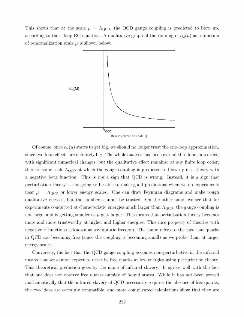
This shows that at the scale µ = ΛQCD, the QCD gauge coupling is predicted to blow up,

according to the 1-loop RG equation. A qualitative graph of the running of αs(µ) as a function

of renormalization scale µ is shown below:

Renormalization scale Q

αS(Q)

ΛQCD

Of course, once αs(µ) starts to get big, we should no longer trust the one-loop approximation,

since two-loop effects are definitely big. The whole analysis has been extended to four-loop order,

with significant numerical changes, but the qualitative effect remains: at any finite loop order,

there is some scale ΛQCD at which the gauge coupling is predicted to blow up in a theory with

a negative beta function. This is not a sign that QCD is wrong. Instead, it is a sign that

perturbation theory is not going to be able to make good predictions when we do experiments

near µ = ΛQCD or lower energy scales. One can draw Feynman diagrams and make rough

qualitative guesses, but the numbers cannot be trusted. On the other hand, we see that for

experiments conducted at characteristic energies much larger than ΛQCD, the gauge coupling is

not large, and is getting smaller as µ gets larger. This means that perturbation theory becomes

more and more trustworthy at higher and higher energies. This nice property of theories with

negative β functions is known as asymptotic freedom. The name refers to the fact that quarks

in QCD are becoming free (since the coupling is becoming small) as we probe them at larger

energy scales.

Conversely, the fact that the QCD gauge coupling becomes non-perturbative in the infrared

means that we cannot expect to describe free quarks at low energies using perturbation theory.

This theoretical prediction goes by the name of infrared slavery. It agrees well with the fact

that one does not observe free quarks outside of bound states. While it has not been proved

mathematically that the infrared slavery of QCD necessarily requires the absence of free quarks,

the two ideas are certainly compatible, and more complicated calculations show that they are

212

plausibly linked. Heuristically, the growth of the QCD coupling means that at very small energies

or large distances, the force between two free color charges is large and constant as the distance

increases. In the early universe, after the temperature dropped below ΛQCD, all quarks and

antiquarks and gluons arranged themselves into color-singlet bound states, and have remained

that way ever since.

An important feature of the renormalization of QCD is that we can actually trade the gauge

coupling as a parameter of the theory for the scale ΛQCD. This is remarkable, since g3 (or

equivalently αs) is a dimensionless coupling, while ΛQCD is a mass scale. If we want, we can

specify how strong the QCD interactions are either by quoting what αs(µ0) is at some specified

µ0, or by quoting what ΛQCD is. This trade of a dimensionless parameter for a mass scale in a

gauge theory is known as dimensional transmutation. Working in a theory with five “active”

quarks u, d, s, c, b (the top quark is treated as part of the unknown theory above the cutoff),

one finds ΛQCD is about 210 MeV. One can also work in an effective theory with only four

active quarks u, d, s, c, in which case ΛQCD is about 290 MeV, or in an effective theory with

only three active quarks u, d, s, in which case ΛQCD is about 330 MeV. Alternatively, αs(mZ) =

0.1181±0.0013. Recently, it has become standard to use this second way of specifying the QCD

coupling strength. These results hold when the details of the cutoff and the renormalization

are treated in the most popular way, called the MS scheme.§ A summary of the experimental

data on the QCD coupling is shown in the figure below (from the 2015 update of the Review of

Particle Properties).

§In this scheme, one cuts off loop momentum integrals by a process known as dimensional regularization, whichcontinuously varies the number of spacetime dimensions infinitesimally away from 4, rather than putting in aparticular cutoff M . Although bizarre physically, this scheme is consistent with gauge invariance and relativelyeasy to calculate in.

213

QCD αs(Mz) = 0.1181 ± 0.0013

pp –> jetse.w. precision fits (NNLO)

0.1

0.2

0.3

αs (Q2)

1 10 100Q [GeV]

Heavy Quarkonia (NLO)

e+e– jets & shapes (res. NNLO)

DIS jets (NLO)

October 2015

τ decays (N3LO)

1000

(NLO

pp –> tt (NNLO)

)(–)

The data determine αS(µ) at a variety of renormalization scales µ from 1.78 GeV up to more

than 1000 GeV. (In the figure, Q was used as the name of the renormalization scale instead of

µ.) The most accurate determinations come from lattice QCD calculations of the mass splittings

in the Υ bottomonium system and from the hadronic branching ratio in τ decays, but other

inputs to the average come from production of jets and tt pairs at hadron colliders, deep inelastic

scattering at the HERA proton-electron collider, and jet production data in e+e− collisions. The

four-loop renormalization group running of αS(µ) with inputs from various widely different µ

are then used to determine the reference value αS(mZ).

We can contrast this situation with the case of QED. For a U(1) group, there is no non-zero

structure constant, so C(G) = 0. Also, since the generator of the group in a representation of

charge Qf is just the 1 × 1 matrix Qf , the index for a fermion with charge Qf is I(Rf ) = Q2f .

Therefore,

b0,QED =4

3

[3nu(2/3)

2 + 3nd(−1/3)2 + nℓ(−1)2]=

16

9nu +

4

9nd +

4

3nℓ, (9.3.29)

where nu is the number of up-type quark flavors (u, c, t), and nd is the number of down-type

quark flavors (d, s, b), and nℓ is the number of charged leptons (e, µ, τ) included in the chosen

effective theory. If we do experiments with a characteristic energy scale me<∼ µ <∼ mµ, then only

the electron itself contributes, and b0,EM = 4/3, so:

de

dlnµ= βe =

e3

16π2

(4

3

)(me

<∼ µ <∼ mµ). (9.3.30)

This corresponds to a very slow running. (Notice that the smaller a gauge coupling is, the

slower it will run.) If we do experiments at characteristic energies that are much less than

214

the electron mass, then the relativistic electron is not included in the effective theory (virtual

electron-positron pairs are less and less important at low energies), so b0,EM = 0, and the electron

charge does not run at all:

de

dlnµ= 0 (µ≪ me). (9.3.31)

This means that QED is not quite “infrared free”, since the effective electromagnetic coupling is

perturbative, but does not get arbitrarily small, at very large distance scales. At extremely high

energies, the coupling e could in principle become very large, because the QED beta function

is always positive. Fortunately, this is predicted to occur only at energy scales far beyond what

we can probe, because e runs very slowly. Furthermore, QED is embedded in a larger, more

complete theory anyway at energy scales in the hundreds of GeV range, so the apparent blowing

up of α = e2/4π much farther in the ultraviolet is just an illusion.

9.4 Parton distribution functions and hadron-hadron scattering

In general, a hadron is a QCD bound state of quarks, anti-quarks, and gluons. The characteristic

size of a hadron, like the proton or antiproton, is always roughly 1/ΛQCD ≈ 10−13 cm, since this

is the scale at which the strongly-interacting particles are confined. In general, the point-like

quark, antiquark, and gluon parts of a hadron are called partons, and the description of hadrons

in terms of them is called the parton model.

Suppose we scatter a hadron off of another particle (which might be another hadron or a

lepton or photon) with a total momentum exchange much larger than ΛQCD. The scattering

can be thought of as a factored into a “hard scattering” of one of the point-like partons, with

the remaining partons as spectators, and “soft” QCD processes that involve exchanges and

radiation of low energy virtual gluons. The hard scattering subprocess takes place on a time

scale much shorter than 1/ΛQCD expressed in seconds. Because of asymptotic freedom, at

higher scattering energies it becomes a better and better approximation to think of the partons

as individual entities that move collectively before and after the scattering, but are free particles

at the moment of scattering. As a first approximation, we can consider only the hard scattering

processes, and later worry about adding on the various soft processes as part of the higher-order

corrections. This way of thinking about things allows us to compute cross-sections for hadron

scattering by first calculating the partonic cross-sections leading to a desired final state, and

then combining them with information about the multiplicity and momentum distributions of

partons within the hadronic bound states.

For example, suppose we want to calculate the scattering of a proton and antiproton. This

215

involves the following 2→2 partonic subprocesses:

qq → qq, qq′ → qq′, qq → qq, qq′ → qq′, (9.4.1)

qq → gg, qq → qq, qq → q′q′, qq′ → qq′, (9.4.2)

qg → qg, qg → qg, gg → gg, gg → qq. (9.4.3)

where g is a gluon and q is any fixed quark flavor and q′ is any quark flavor that is definitely

different from q. Let the center-of-mass energy of the proton and antiproton be called√s. Each

parton only carries a fraction of the energy of the energy of the proton it belongs to, so the

partonic center-of-mass energy, call it√s, will be significantly less than

√s. One often uses

hatted Mandelstam variables s, t and u for the partonic scattering event. If√s≫ ΛQCD, then

the two partons in the final state will be sufficiently energetic that they can usually escape

from most or all of the spectator quarks and gluons before hadronizing (forming bound states).

However, before traveling a distance 1/ΛQCD, they must rearrange themselves into color-singlet

combinations, possibly by creating quark-antiquark or gluon-antigluon pairs out of the vacuum.

This hadronization process can be quite complicated, but will usually result in a jet of hadronic

particles moving with roughly the same 4-momentum as the parton that was produced. So, all

of the partonic process cross-sections in eq. (9.4.3) contribute to the observable cross-section for

the process:

pp→ jj +X, (9.4.4)

where j stands for a jet. The X stands for “anything”, and includes stray hadronic junk left

over from the original proton and antiproton. Similarly, partonic hard scatterings like:

qq → q′q′g, qg → qgg, qg → qgg, gg → ggg, (9.4.5)

and so on, will contribute to an observable cross-section for

pp→ jjj +X. (9.4.6)

The 2 × 2 hard scattering processes can also contribute to this process if one of the final state

partons hadronizes by splitting into two jets, or if there is an additional jet from the initial state.

In order to use the calculation of cross-sections for partonic processes like eq. (9.4.3) to obtain

measurable cross-sections, we need to know how likely it is to have a given parton inside the

initial-state hadron with a given 4-momentum. Since we are mostly interested in high-energy

scattering problems, we can make things simple, and treat the hadron and all of its constituents

as nearly massless. (For the proton, this means that we are assuming that√s≫ mp ≈ 1 GeV.)

216

Suppose we therefore take the total 4-momentum of the hadron h in an appropriate Lorentz

frame to be:

pµh = (E, 0, 0, E). (9.4.7)

This is sometimes called the “infinite momentum frame”, even though E is finite, since E ≫ mp.

Consider a parton constituent A (a quark, antiquark, or gluon) that carries a fraction x of the

hadron’s momentum:

pµA = x(E, 0, 0, E). (9.4.8)

The variable x is a standard notation, and is called the (longitudinal) momentum fraction for

the parton, or Feynman’s x. It is older than QCD, dating back to a time when the proton

was suspected to contain point-like partons with properties that were then obscure. In order to

describe the partonic content of a hadron, one defines:Probability of finding a parton of type A with4-momentum between xpµ and (x+ dx)pµ

inside a hadron h with 4-momentum pµ

= fh

A(x) dx . (9.4.9)

The function fhA(x) is called the parton distribution function or PDF for the parton A in the

hadron h. The parton can be either one of the two or three valence quarks or antiquarks that

are the nominal constituents of the hadron, or one of an indeterminate number of virtual sea

quarks and gluons. Either type of parton can participate in a scattering event.

Hadronic collisions studied in laboratories usually involve protons or antiprotons, so the

PDFs of the proton and antiproton are especially interesting. The proton is nominally a bound

state of three valence quarks, namely two up quarks and one down quark, so we are certainly

interested in the up-quark and down-quark distribution functions

f pu(x) and f p

d (x).

The proton also contains virtual gluons, implying a gluon distribution function:

f pg (x). (9.4.10)

Furthermore, there are always virtual quark-antiquark pairs within the proton. This adds ad-

ditional contributions to f pu(x) and f

pd (x), and also means that there is a non-zero probability

of finding antiup, antidown, or strange or antistrange quarks:

f pu(x), f p

d(x), f p

s (x), f ps (x). (9.4.11)

These parton distribution functions are implicitly summed over color and spin. So f pu(x) tells us

the probability of finding an up quark with the given momentum fraction x and any color and

217

spin. Since the gluon is its own antiparticle (it lives in the adjoint representation of the gauge

group, which is always a real representation), there is not a separate f pg (x).

Although the charm, bottom and top quarks are heavier than the proton, virtual charm-

anticharm, bottom-antibottom, and top-antitop pairs can exist as long as their total energy does

not exceed mp. This can happen because, as virtual particles, they need not be on-shell. So, one

can even talk about the parton distribution functions f pc (x), f

pc (x), f

pb (x), f

p

b(x), f p

t (x), fp

t(x).

Fortunately, these are small so one can often neglect them, although they can be important for

processes involving charm or bottom quarks in the final state.

Given the PDFs for the proton, the PDFs for the antiproton follow immediately from the

fact that it is the proton’s antiparticle. The probability of finding a given parton in the proton

with a given x is the same as the probability of finding the corresponding antiparton in the

antiproton with the same x. Therefore, if we know the PDFs for the proton, there is no new

information in the PDFs for the antiproton. We can just describe everything having to do with

proton and antiproton collisions in terms of the proton PDFs. To simplify the notation, it is

traditional to write the proton and antiproton PDFs as:

g(x) = f pg (x) = f p

g (x), (9.4.12)

u(x) = f pu(x) = f p

u(x), (9.4.13)

d(x) = f pd (x) = f p

d(x), (9.4.14)

u(x) = f pu(x) = f p

u(x), (9.4.15)

d(x) = f p

d(x) = f p

d (x), (9.4.16)

s(x) = f ps (x) = f p

s (x), (9.4.17)

s(x) = f ps (x) = f p

s (x). (9.4.18)

The PDFs are also functions of another parameter Q (sometimes denoted µ or µF ), known

as the factorization scale. The factorization scale can be thought of as the energy scale that

serves as the boundary between what is treated as the short-distance hard partonic process

and what is taken to be part of the long-distance physics associated with hadronization. The

choice of the factorization scale is an arbitrary one, and in principle the final result should not

depend on it, just like the choice of renormalization scale discussed in section 9.3 is arbitrary.

It is very common to choose the factorization scale equal to the renormalization scale, although

this is not mandatory. (When they are distinguished in the literature, some authors use Q

for the renormalization scale and µ for the factorization scale, and some use the reverse as we

have here. Some use the same letter for both, especially when choosing them to be the same

numerically.) The PDFs have a mild logarithmic dependence on the choice of factorization scale

Q, which can be computed in perturbation theory by a set of equations known as the DGLAP

218

(Dokshitzer–Gribov–Lipatov–Altarelli–Parisi) equations. So they are really functions g(x,Q2)

etc., although the Q-dependence is often left implicit for brevity, as we will mostly do below.

It is usual to choose the factorization scale Q to be comparable to some energy scale relevant

to the physical process of interest. For example, in deeply inelastic scattering of leptons off of

protons, with momentum transfer to the scattered quark qµ, the factorization scale is typically

chosen as Q2 = −q2. This Q2 is positive, since qµ is a spacelike vector. When producing a pair

of heavy particles with some mass m, it is common to choose Q = m or some fraction thereof.

After having completed a calculation, one often varies the renormalization and factorization

scales (either together or independently) over a range (say, from Q = m/4 to Q = 2m in the

case just mentioned) to see how the cross-section or other observables that resulted from the

calculation vary. This is a test of the accuracy of the perturbation theory calculation, since in

principle if one could calculate exactly rather than to some low order in perturbation theory,

the results should not depend on either scale choice at all.

In the proton, antiquarks are always virtual, and so must be accompanied by a quark with

the same flavor. This implies that if we add up all the up quarks found in the proton, and

subtract all the anti-ups, we must find a total of 2 quarks:∫ 1

0dx

[u(x,Q2)− u(x,Q2)

]= 2. (9.4.19)

Similarly, summing over all x the probability of finding a down quark with a given x, and

subtracting the same thing for anti-downs, one has:∫ 1

0dx

[d(x,Q2)− d(x,Q2)

]= 1. (9.4.20)

Most of the strange quarks in the proton come from the process of a virtual gluon splitting into

a strange and anti-strange pair. Since the virtual gluon treats quarks and antiquarks on an

equal footing, for every strange quark with a given x, there should be† an equal probability of

finding an antistrange with the same x:

s(x,Q2) = s(x,Q2). (9.4.21)

The up-quark PDF can be thought of as divided into a contribution uv(x) from the two valence

quarks, and a contribution us(x) from the sea (non-valence) quarks that are accompanied by an

anti-up. (Here and below the factorization scale dependence is left implicit, for brevity.) So we

have:

u(x) = uv(x) + us(x), us(x) = u(x); (9.4.22)

d(x) = dv(x) + ds(x), ds(x) = d(x). (9.4.23)

†Although QCD interactions do not change quark flavors, there is a small strangeness violation in the weakinteractions, so the following rule is not quite exact.

219

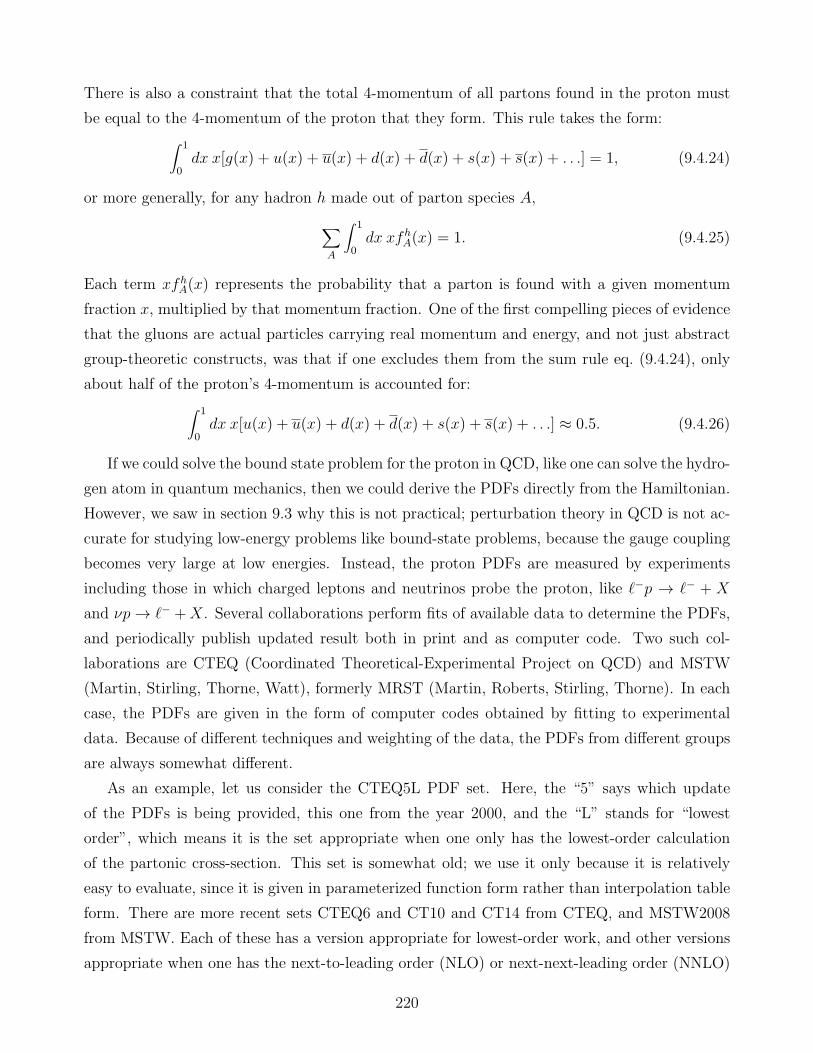
There is also a constraint that the total 4-momentum of all partons found in the proton must

be equal to the 4-momentum of the proton that they form. This rule takes the form:

∫ 1

0dx x[g(x) + u(x) + u(x) + d(x) + d(x) + s(x) + s(x) + . . .] = 1, (9.4.24)

or more generally, for any hadron h made out of parton species A,

∑

A

∫ 1

0dx xfh

A(x) = 1. (9.4.25)

Each term xfhA(x) represents the probability that a parton is found with a given momentum

fraction x, multiplied by that momentum fraction. One of the first compelling pieces of evidence

that the gluons are actual particles carrying real momentum and energy, and not just abstract

group-theoretic constructs, was that if one excludes them from the sum rule eq. (9.4.24), only

about half of the proton’s 4-momentum is accounted for:

∫ 1

0dx x[u(x) + u(x) + d(x) + d(x) + s(x) + s(x) + . . .] ≈ 0.5. (9.4.26)

If we could solve the bound state problem for the proton in QCD, like one can solve the hydro-

gen atom in quantum mechanics, then we could derive the PDFs directly from the Hamiltonian.

However, we saw in section 9.3 why this is not practical; perturbation theory in QCD is not ac-

curate for studying low-energy problems like bound-state problems, because the gauge coupling

becomes very large at low energies. Instead, the proton PDFs are measured by experiments

including those in which charged leptons and neutrinos probe the proton, like ℓ−p → ℓ− + X

and νp→ ℓ− +X. Several collaborations perform fits of available data to determine the PDFs,

and periodically publish updated result both in print and as computer code. Two such col-

laborations are CTEQ (Coordinated Theoretical-Experimental Project on QCD) and MSTW

(Martin, Stirling, Thorne, Watt), formerly MRST (Martin, Roberts, Stirling, Thorne). In each

case, the PDFs are given in the form of computer codes obtained by fitting to experimental

data. Because of different techniques and weighting of the data, the PDFs from different groups

are always somewhat different.

As an example, let us consider the CTEQ5L PDF set. Here, the “5” says which update

of the PDFs is being provided, this one from the year 2000, and the “L” stands for “lowest

order”, which means it is the set appropriate when one only has the lowest-order calculation

of the partonic cross-section. This set is somewhat old; we use it only because it is relatively

easy to evaluate, since it is given in parameterized function form rather than interpolation table

form. There are more recent sets CTEQ6 and CT10 and CT14 from CTEQ, and MSTW2008

from MSTW. Each of these has a version appropriate for lowest-order work, and other versions

appropriate when one has the next-to-leading order (NLO) or next-next-leading order (NNLO)

220

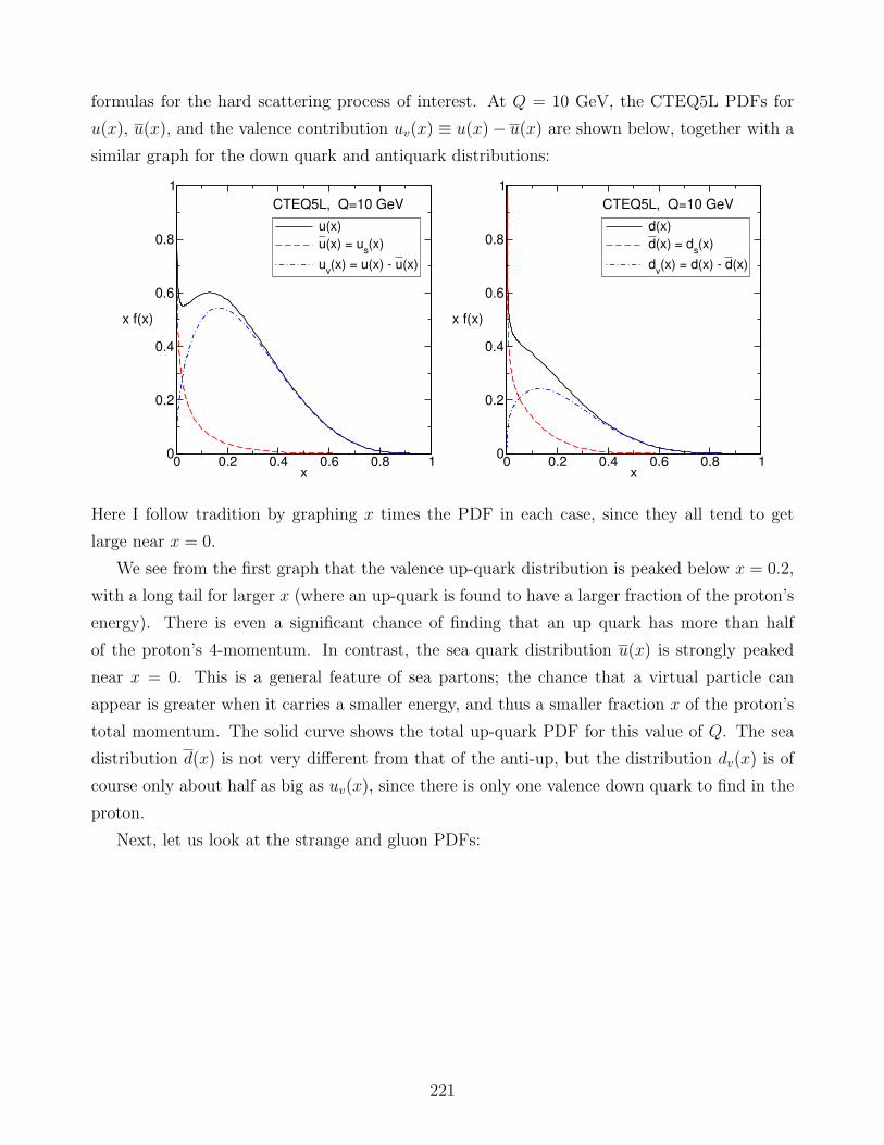
formulas for the hard scattering process of interest. At Q = 10 GeV, the CTEQ5L PDFs for

u(x), u(x), and the valence contribution uv(x) ≡ u(x)− u(x) are shown below, together with a

similar graph for the down quark and antiquark distributions:

0 0.2 0.4 0.6 0.8 1x

0

0.2

0.4

0.6

0.8

1

x f(x)

u(x)

u(x) = us(x)

uv(x) = u(x) - u(x)

CTEQ5L, Q=10 GeV

0 0.2 0.4 0.6 0.8 1x

0

0.2

0.4

0.6

0.8

1

x f(x)

d(x)

d(x) = ds(x)

dv(x) = d(x) - d(x)

CTEQ5L, Q=10 GeV

Here I follow tradition by graphing x times the PDF in each case, since they all tend to get

large near x = 0.

We see from the first graph that the valence up-quark distribution is peaked below x = 0.2,

with a long tail for larger x (where an up-quark is found to have a larger fraction of the proton’s

energy). There is even a significant chance of finding that an up quark has more than half

of the proton’s 4-momentum. In contrast, the sea quark distribution u(x) is strongly peaked

near x = 0. This is a general feature of sea partons; the chance that a virtual particle can

appear is greater when it carries a smaller energy, and thus a smaller fraction x of the proton’s

total momentum. The solid curve shows the total up-quark PDF for this value of Q. The sea

distribution d(x) is not very different from that of the anti-up, but the distribution dv(x) is of

course only about half as big as uv(x), since there is only one valence down quark to find in the

proton.

Next, let us look at the strange and gluon PDFs:

221

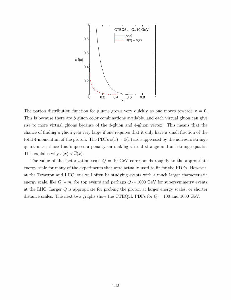
0 0.2 0.4 0.6 0.8 1x

0

0.2

0.4

0.6

0.8

1

x f(x)

g(x)

s(x) = s(x)

CTEQ5L, Q=10 GeV

The parton distribution function for gluons grows very quickly as one moves towards x = 0.

This is because there are 8 gluon color combinations available, and each virtual gluon can give

rise to more virtual gluons because of the 3-gluon and 4-gluon vertex. This means that the

chance of finding a gluon gets very large if one requires that it only have a small fraction of the

total 4-momentum of the proton. The PDFs s(x) = s(x) are suppressed by the non-zero strange

quark mass, since this imposes a penalty on making virtual strange and antistrange quarks.

This explains why s(x) < d(x).

The value of the factorization scale Q = 10 GeV corresponds roughly to the appropriate

energy scale for many of the experiments that were actually used to fit for the PDFs. However,

at the Tevatron and LHC, one will often be studying events with a much larger characteristic

energy scale, like Q ∼ mt for top events and perhaps Q ∼ 1000 GeV for supersymmetry events

at the LHC. Larger Q is appropriate for probing the proton at larger energy scales, or shorter

distance scales. The next two graphs show the CTEQ5L PDFs for Q = 100 and 1000 GeV:

222

0 0.2 0.4 0.6 0.8 1x

0

0.2

0.4

0.6

0.8

1

x f(x)

CTEQ5L, Q=100 GeVg

u

d

u

d

0 0.2 0.4 0.6 0.8 1x

0

0.2

0.4

0.6

0.8

1

x f(x)

CTEQ5L, Q=1000 GeVg

ud

u

d

As Q increases from Q = 100 to 1000 GeV, the PDFs become larger at very small x (although

this is hard to see from the graphs), but smaller for x >∼ 0.015 for gluons and x >∼ 0.04 for quarks.

More generally, the variation with Q can be made quantitative using the DGLAP equations,

which are built into the computer codes that provide the parton distributions as a function of

x and Q.

Now suppose we have available a set of PDFs, and let us see how to use them to get a cross-

section. Consider scattering two hadrons h and h′, and let the partonic differential cross-sections

for the desired final state X be

dσ(ab→ X) (9.4.27)

for any two partons a (to be taken from h) and b (from h′). The hat is used as a reminder that

this is a partonic process. If X has two particles 1,2 in it, then one defines partonic Mandelstam

variables:

s = (pa + pb)2, (9.4.28)

t = (pa − k1)2, (9.4.29)

u = (pa − k2)2. (9.4.30)

Let us work in the center-of-momentum frame, with approximately massless hadrons and par-

tons, so that

pµh = (E, 0, 0, E), (9.4.31)

pµh′ = (E, 0, 0,−E). (9.4.32)

223

Then we can define a Feynman x for each of the initial-state partons, xa and xb, so:

pµa = xa(E, 0, 0, E), (9.4.33)

pµb = xb(E, 0, 0,−E). (9.4.34)

It follows that, with s = (ph + ph′)2 for the whole hadronic event,

s = (xa + xb)2E2 − (xa − xb)E2 = 4xaxbE

2 = sxaxb. (9.4.35)

Here s is determined by the collider [(1960 GeV)2 at the Tevatron and (13 TeV)2 presently at

the LHC], while s is different for each event. Now, to find the total cross-section to produce the

final state X in h, h′ collisions, we should multiply the partonic cross-section by the probabilities

of finding in h a parton a with momentum fraction in the range xa to xa + dxa and the same

probability for parton b in h′; then integrate over all possible xa and xb, and then sum over all

the different parton species a and b. The result is:

dσ(hh′ → X) =∑

a,b

∫ 1

0dxa

∫ 1

0dxb dσ(ab→ X) fh

a (xa) fh′

b (xb). (9.4.36)

This integration is done by computer, using PDFs with Q chosen equal to some energy char-

acteristic of the event. The partonic differential cross-section dσ(ab → X) depends on the

momentum fractions xa and xb through pµa = xap

µh and pµb = xbp

µh′ , with p

µh and pµh′ controlled or

known by the experimenter.

9.5 Top-antitop production in pp and pp collisions

As an example, let us consider top-antitop production, first at the Tevatron. The parton-level

processes that can contribute to this are, with the first parton taken to be from the proton and

the second from the antiproton:

uu→ tt, dd→ tt, gg → tt, dd→ tt, uu→ tt, ss→ tt, ss→ tt. (9.5.1)

These are listed in the order of their numerical importance in contributing to the total cross-

section for tt at the Tevatron. Notice that the most likely thing is to find a quark in the proton

and an antiquark in the anti-proton, but there is also a small but non-zero probability of finding

an anti-quark in the proton, and a quark in the anti-proton. All of the processes involving quark

and antiquark in the initial state involve the same parton-level cross-section

dσ(qq → tt)

dt. (9.5.2)

224

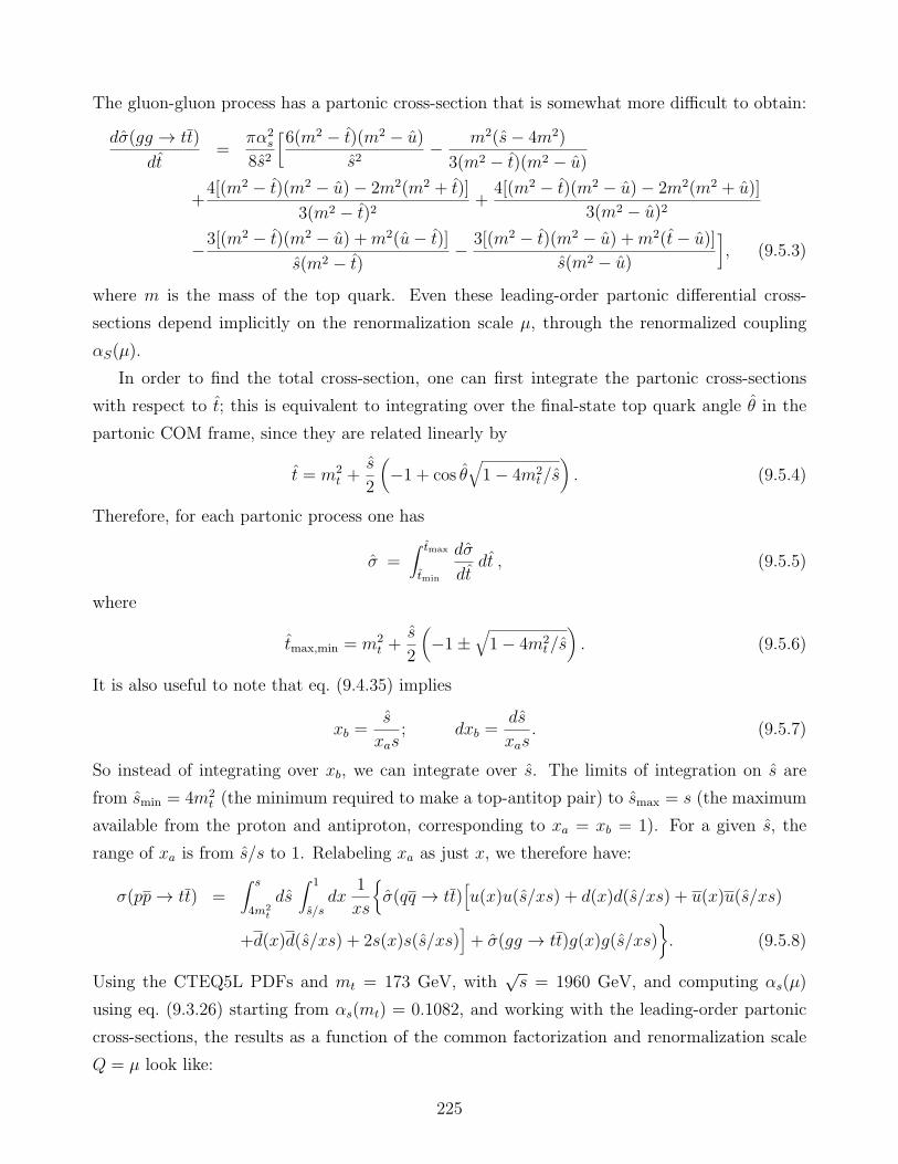
The gluon-gluon process has a partonic cross-section that is somewhat more difficult to obtain:

dσ(gg → tt)

dt=

πα2s

8s2

[6(m2 − t)(m2 − u)

s2− m2(s− 4m2)

3(m2 − t)(m2 − u)

+4[(m2 − t)(m2 − u)− 2m2(m2 + t)]

3(m2 − t)2 +4[(m2 − t)(m2 − u)− 2m2(m2 + u)]

3(m2 − u)2

−3[(m2 − t)(m2 − u) +m2(u− t)]s(m2 − t) − 3[(m2 − t)(m2 − u) +m2(t− u)]

s(m2 − u)

], (9.5.3)

where m is the mass of the top quark. Even these leading-order partonic differential cross-

sections depend implicitly on the renormalization scale µ, through the renormalized coupling

αS(µ).

In order to find the total cross-section, one can first integrate the partonic cross-sections

with respect to t; this is equivalent to integrating over the final-state top quark angle θ in the

partonic COM frame, since they are related linearly by

t = m2t +

s

2

(−1 + cos θ

√1− 4m2

t/s). (9.5.4)

Therefore, for each partonic process one has

σ =∫ tmax

tmin

dσ

dtdt , (9.5.5)

where

tmax,min = m2t +

s

2

(−1±

√1− 4m2

t/s). (9.5.6)

It is also useful to note that eq. (9.4.35) implies

xb =s

xas; dxb =

ds

xas. (9.5.7)

So instead of integrating over xb, we can integrate over s. The limits of integration on s are

from smin = 4m2t (the minimum required to make a top-antitop pair) to smax = s (the maximum

available from the proton and antiproton, corresponding to xa = xb = 1). For a given s, the

range of xa is from s/s to 1. Relabeling xa as just x, we therefore have:

σ(pp→ tt) =∫ s

4m2t

ds∫ 1

s/sdx

1

xs

σ(qq → tt)

[u(x)u(s/xs) + d(x)d(s/xs) + u(x)u(s/xs)

+d(x)d(s/xs) + 2s(x)s(s/xs)]+ σ(gg → tt)g(x)g(s/xs)

. (9.5.8)

Using the CTEQ5L PDFs and mt = 173 GeV, with√s = 1960 GeV, and computing αs(µ)

using eq. (9.3.26) starting from αs(mt) = 0.1082, and working with the leading-order partonic

cross-sections, the results as a function of the common factorization and renormalization scale

Q = µ look like:

225

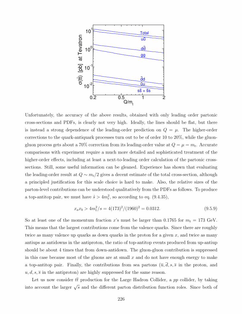
0.2 0.5 1 2Q/m

t

10-2

10-1

100

101

σ(tt

) [pb] a

t T

evatr

on

Total

uu

uudd

dd

gg

ss + ss- -

-

-

-

-

Unfortunately, the accuracy of the above results, obtained with only leading order partonic

cross-sections and PDFs, is clearly not very high. Ideally, the lines should be flat, but there

is instead a strong dependence of the leading-order prediction on Q = µ. The higher-order

corrections to the quark-antiquark processes turn out to be of order 10 to 20%, while the gluon-

gluon process gets about a 70% correction from its leading-order value at Q = µ = mt. Accurate

comparisons with experiment require a much more detailed and sophisticated treatment of the

higher-order effects, including at least a next-to-leading order calculation of the partonic cross-

sections. Still, some useful information can be gleaned. Experience has shown that evaluating

the leading-order result at Q ∼ mt/2 gives a decent estimate of the total cross-section, although

a principled justification for this scale choice is hard to make. Also, the relative sizes of the

parton-level contributions can be understood qualitatively from the PDFs as follows. To produce

a top-antitop pair, we must have s > 4m2t , so according to eq. (9.4.35),

xaxb > 4m2t/s = 4(173)2/(1960)2 = 0.0312. (9.5.9)

So at least one of the momentum fraction x’s must be larger than 0.1765 for mt = 173 GeV.

This means that the largest contributions come from the valence quarks. Since there are roughly

twice as many valence up quarks as down quarks in the proton for a given x, and twice as many

antiups as antidowns in the antiproton, the ratio of top-antitop events produced from up-antiup

should be about 4 times that from down-antidown. The gluon-gluon contribution is suppressed

in this case because most of the gluons are at small x and do not have enough energy to make

a top-antitop pair. Finally, the contributions from sea partons (u, d, s, s in the proton, and

u, d, s, s in the antiproton) are highly suppressed for the same reason.

Let us now consider tt production for the Large Hadron Collider, a pp collider, by taking

into account the larger√s and the different parton distribution function roles. Since both of

226

the initial-state hadrons are protons, the formula for the total cross-section is now:

σ(pp→ tt) =∫ s

4m2t

ds∫ 1

s/sdx

1

xs

σ(qq → tt)

[2u(x)u(s/xs) + 2d(x)d(s/xs) + 2s(x)s(s/xs)

]

+σ(gg → tt) g(x)g(s/xs). (9.5.10)

The factors of 2 are present because each proton can contribute either the quark, or the an-

tiquark; then the contribution of the other proton is fixed. The gluon-gluon contribution has

the same form as in pp collisions, because the gluon distribution is identical in protons and in

antiprotons.

Numerically integrating the above formula with a computer using the CTEQ5L PDFs, one

finds the leading order results shown below, as a function of the common factorization and

renormalization scale Q = µ, for the case of√s = 14 TeV:

0.2 0.5 1 2Q/m

t

100

101

102

103

σ(tt

) [

pb

] a

t 1

4 T

eV

LH

C

Total

uu + uu

cc + cc-

dd + dd

gg

ss + ss- -

-

-

-

-

-

Again these leading-order results are highly dependent onQ = µ, and subject to large corrections

at next-to-leading order and beyond. The most striking feature of the LHC result is that in

contrast to the Tevatron situation, the gluon-gluon partonic contribution is dominant over the

quark-antiquark contributions for the LHC. This is partly because all of the quark-antiquark

contributions now require a sea antiquark PDF, but that is not the main reason. The really

important effect is that at very high energies like at the LHC, the top quark can be considered

light (!) and so one can make them using partons with much lower x. For example, with√s = 14

TeV, the kinematic constraint on the longitudinal momentum fractions becomes

xaxb > 4(173)2/(14000)2 = 0.000611, (9.5.11)

so that now the smaller one can be as low as 0.0247. At low x, we saw above that the gluon

distribution function is very large; one has plenty of gluons available with less than 1/10 of the

227

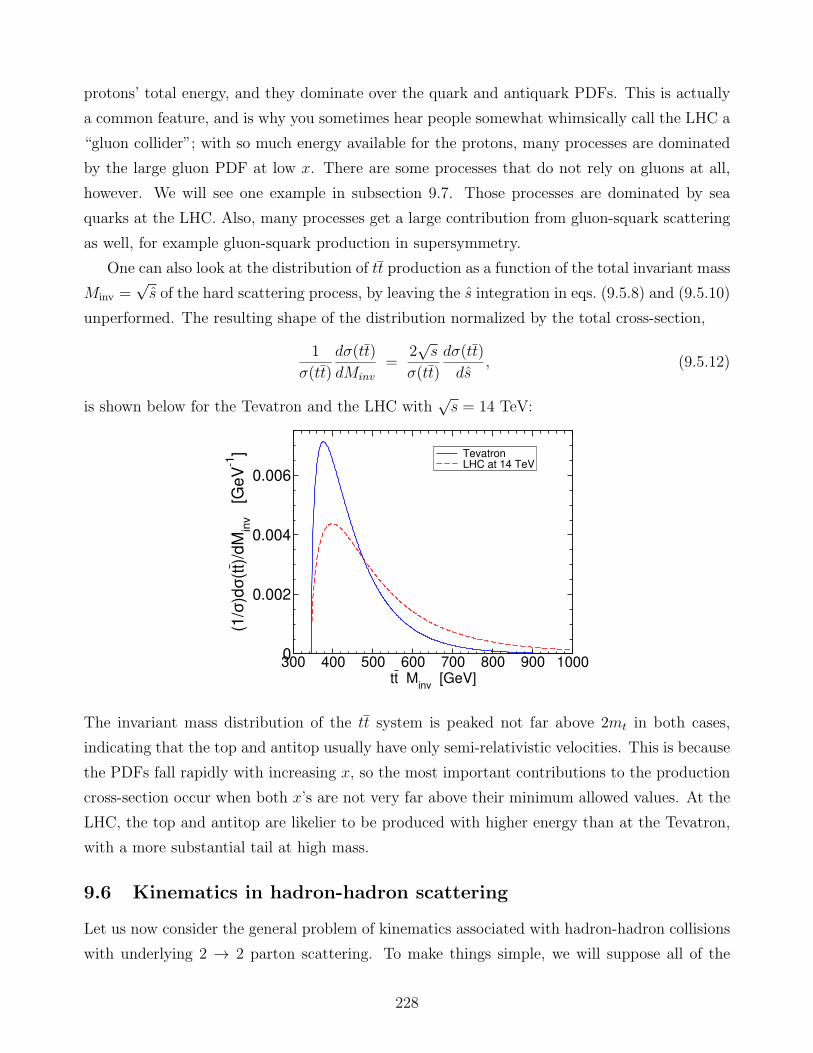
protons’ total energy, and they dominate over the quark and antiquark PDFs. This is actually

a common feature, and is why you sometimes hear people somewhat whimsically call the LHC a

“gluon collider”; with so much energy available for the protons, many processes are dominated

by the large gluon PDF at low x. There are some processes that do not rely on gluons at all,

however. We will see one example in subsection 9.7. Those processes are dominated by sea

quarks at the LHC. Also, many processes get a large contribution from gluon-squark scattering

as well, for example gluon-squark production in supersymmetry.

One can also look at the distribution of tt production as a function of the total invariant mass

Minv =√s of the hard scattering process, by leaving the s integration in eqs. (9.5.8) and (9.5.10)

unperformed. The resulting shape of the distribution normalized by the total cross-section,

1

σ(tt)

dσ(tt)

dMinv

=2√s

σ(tt)

dσ(tt)

ds, (9.5.12)

is shown below for the Tevatron and the LHC with√s = 14 TeV:

300 400 500 600 700 800 900 1000tt M

inv [GeV]

0

0.002

0.004

0.006

(1/σ

)dσ(

tt)/

dM

inv

[G

eV

-1] Tevatron

LHC at 14 TeV

The invariant mass distribution of the tt system is peaked not far above 2mt in both cases,

indicating that the top and antitop usually have only semi-relativistic velocities. This is because

the PDFs fall rapidly with increasing x, so the most important contributions to the production

cross-section occur when both x’s are not very far above their minimum allowed values. At the

LHC, the top and antitop are likelier to be produced with higher energy than at the Tevatron,

with a more substantial tail at high mass.

9.6 Kinematics in hadron-hadron scattering

Let us now consider the general problem of kinematics associated with hadron-hadron collisions

with underlying 2 → 2 parton scattering. To make things simple, we will suppose all of the

228

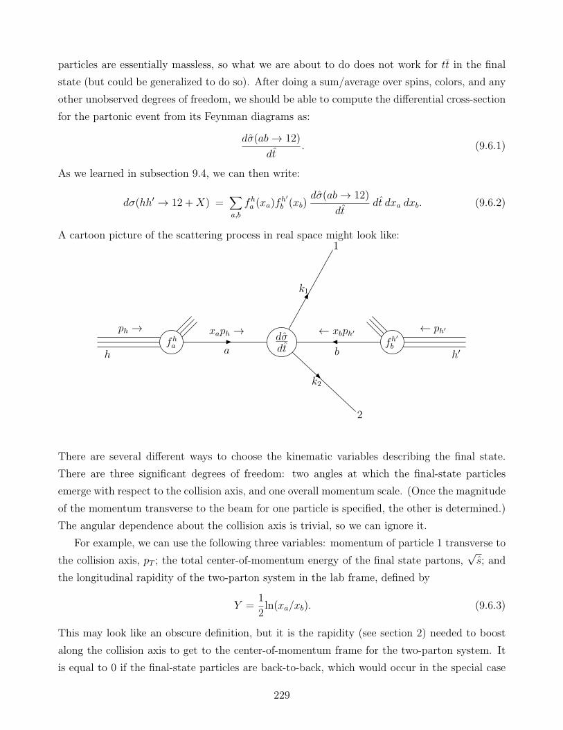
particles are essentially massless, so what we are about to do does not work for tt in the final

state (but could be generalized to do so). After doing a sum/average over spins, colors, and any

other unobserved degrees of freedom, we should be able to compute the differential cross-section

for the partonic event from its Feynman diagrams as:

dσ(ab→ 12)

dt. (9.6.1)

As we learned in subsection 9.4, we can then write:

dσ(hh′ → 12 +X) =∑

a,b

fha (xa)f

h′

b (xb)dσ(ab→ 12)

dtdt dxa dxb. (9.6.2)

A cartoon picture of the scattering process in real space might look like:

fha fh′

bdσdt

ph → ← ph′

h h′

xaph → ← xbph′

a b

1

2

k1

k2

There are several different ways to choose the kinematic variables describing the final state.

There are three significant degrees of freedom: two angles at which the final-state particles

emerge with respect to the collision axis, and one overall momentum scale. (Once the magnitude

of the momentum transverse to the beam for one particle is specified, the other is determined.)

The angular dependence about the collision axis is trivial, so we can ignore it.

For example, we can use the following three variables: momentum of particle 1 transverse to

the collision axis, pT ; the total center-of-momentum energy of the final state partons,√s; and

the longitudinal rapidity of the two-parton system in the lab frame, defined by

Y =1

2ln(xa/xb). (9.6.3)

This may look like an obscure definition, but it is the rapidity (see section 2) needed to boost

along the collision axis to get to the center-of-momentum frame for the two-parton system. It

is equal to 0 if the final-state particles are back-to-back, which would occur in the special case

229

that the initial-state partons have the same energy in the lab frame. Instead of the variables

(xa, xb, t), we can use the more directly observable variables (s, p2T , Y ), or perhaps some subset of

these with the others integrated over. Working in the center-of-momentum frame of the partons,

we can write:

pµa = (E, 0, 0, E), (9.6.4)

pµb = (E, 0, 0,−E), (9.6.5)

kµ1 = (E, 0, pT ,√E2 − p2T ), (9.6.6)

kµ2 = (E, 0,−pT ,−√E2 − p2T ), (9.6.7)

with

s = 4E2 = xaxbs, (9.6.8)

from which it follows that

t = (pa − k1)2 =s

2

(1 +

√1− 4p2T/s

), (9.6.9)

u = (pa − k2)2 =s

2

(1−

√1− 4p2T/s

), (9.6.10)

and so

p2T =tu

s= − t(sxaxb + t)

sxaxb, (9.6.11)

where the last equality uses u = −s− t = −sxaxb− t for massless particles. Making the change

of variables (xa, xb, t) to (s, p2T , Y ) for a differential cross-section requires

dt dxa dxb = J ds d(p2T ) dY, (9.6.12)

where J is the determinant of the Jacobian matrix of the transformation. Evaluating it, by

taking the inverse of the determinant of its inverse, one finds:

J =

∣∣∣∣∣∂(s, p2T , Y )

∂(t, xa, xb)

∣∣∣∣∣

−1

=xaxb

s+ 2t. (9.6.13)

Therefore, eq. (9.6.2) becomes:

dσ(hh′ → 12 +X)

ds d(p2T ) dY=

xaxb

s+ 2t

∑

a,b

fha (xa)f

h′

b (xb)dσ(ab→ 12)

dt, (9.6.14)

where the variables xa, xb, t on the right-hand side are understood to be determined in terms of

s, p2T and Y by eqs. (9.6.8), (9.6.11), and (9.6.3).

230

9.7 Drell-Yan scattering (ℓ+ℓ− production in hadron collisions)

As an example, let us consider the process of Drell-Yan scattering, which is the production of

lepton pairs in hadron-hadron collisions through a virtual photon:

hh′ → ℓ+ℓ−. (9.7.1)

This does not involve QCD as the hard partonic scattering, since the leptons ℓ = e, µ, or τ are

singlets under SU(3)c color. However, it still depends on QCD, because to evaluate it we need

to know the PDFs for the quarks inside the hadrons. Since gluons have no electric charge and

do not couple to photons, the underlying partonic process is always:

qq → ℓ+ℓ−. (9.7.2)

with the q coming from either h or h′. The cross-section for this, for√s≪ mZ and not near a

resonance, can be obtained by exactly the same methods as in 5.2.1 for e+e− → µ+µ−; we just

need to remember to use the charge of the quark Qq instead of the charge of the electron, and

to average over initial-state colors. The latter effect leads to a suppression of 1/3; there is no

reaction if the colors do not match. One finds that the differential partonic cross-section is:

dσ(qq → ℓ+ℓ−)

dt=

2πα2Q2q(t

2 + u2)

3s4. (9.7.3)

Therefore, using u = −s − t for massless scattering, and writing separate contributions from

finding the quark, and the antiquark, in h:

dσ(hh′ → ℓ+ℓ−)

ds dp2T dY=

2πα2

3

t2 + (s+ t)2

s4(s+ 2t)xaxb

∑

q

Q2q

[fhq (xa)f

h′

q (xb) + fhq (xa)f

h′

q (xb)]. (9.7.4)

This can be used to make a prediction for the experimental distribution of events with respect

to each of s, pT , and Y .

Alternatively, we can choose to integrate the partonic differential cross-section with respect

to t first. Since t determines the scattering angle with respect to the collision axis, this will

eliminate the integration over p2T . The total partonic cross-section obtained by integrating

eq. (9.7.3) is:

σ(qq → ℓ+ℓ−) =4πα2Q2

q

9s. (9.7.5)

Therefore we get:

dσ(hh′ → ℓ+ℓ−) = dxadxb4πα2

9s

∑

q

Q2q

[fhq (xa)f

h′

q (xb) + fhq (xa)f

h′

q (xb)]. (9.7.6)

231

Now making the change of variables from (xa, xb) to (s, Y ) requires:

dxadxb =

∣∣∣∣∣∂(s, Y )

∂(xa, xb)

∣∣∣∣∣

−1

ds dY =ds dY

s, (9.7.7)

we therefore have:

dσ(hh′ → ℓ+ℓ−)

ds dY=

4πα2

9ss

∑

q

Q2q

[fhq (xa)f

h′

q (xb) + fhq (xa)f

h′

q (xb)]. (9.7.8)

Still another way to present the result is to leave only s unintegrated, by again first integrating

the partonic differential cross-section with respect to t, and then trading one of the Feynman-x

variables for s, and do the remaining x-integration. This is how we wrote the top-antitop total

cross-section. The Jacobian factor in the change of variables from (xa, xb)→ (xa, s) is now:

dxa dxb =

∣∣∣∣∣∂s

∂xb

∣∣∣∣∣

−1

dxa ds =dxa ds

xas. (9.7.9)

Using this in eq. (9.7.6) now gives, after replacing xa by x and integrating:

dσ(hh′ → ℓ+ℓ−)

ds=

4πα2

9s2∑

q

Q2q

∫ 1

s/sdx

s

xs

[fhq (x)f

h′

q (s/xs) + fhq (x)f

h′

q (s/xs)]. (9.7.10)

This version makes a nice prediction that is (almost) independent of the actual parton distri-

bution functions. The right-hand side could have depended on both s and s in an arbitrary

way, but to the extent that the PDFs are independent of Q, we see that it is predicted to scale

like 1/s2 times some function of the ratio s/s. Since the PDFs run slowly with Q, this is a

reasonably good prediction. Drell-Yan scattering has been studied in hh′ = pp, pp, π±p, and

K±p scattering experiments, and in each case the results indeed satisfy the scaling law:

s2dσ(hh′ → ℓ+ℓ−)

ds= Fhh′(s/s) (9.7.11)

to a very good approximation, for low s not near a resonance. Furthermore, the functions Fhh′

gives information about the PDFs.

Because of the relatively clean signals of muons in particle detectors, the Drell-Yan process

pp→ µ−µ+ +X or pp→ µ−µ+ +X (9.7.12)

is often one of the first things one studies at a hadron collider to make sure everything is working

correctly and understood. It also provides a test of the PDFs, especially at small x.

For larger√s, one must take into account the s-channel Feynman diagram with a Z boson

in place of the virtual photon. The resulting cross-section can be obtained from eq. (9.7.10) by

replacing

4πα2

9s2∑

q

Q2q →

4πα2

9

∑

q

[Q2

q

s2+

(V 2q + A2

q)(V2ℓ + A2

ℓ)

(s−m2Z)

2 +m2ZΓ

2Z

− 2QqVqVℓ(1−m2Z/s)

(s−m2Z)

2 +m2ZΓ

2Z

], (9.7.13)

232

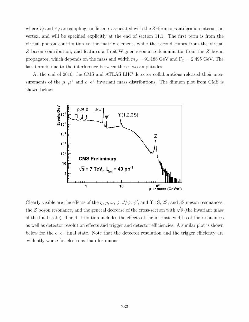
where Vf and Af are coupling coefficients associated with the Z–fermion–antifermion interaction

vertex, and will be specified explicitly at the end of section 11.1. The first term is from the

virtual photon contribution to the matrix element, while the second comes from the virtual

Z boson contribution, and features a Breit-Wigner resonance denominator from the Z boson

propagator, which depends on the mass and width mZ = 91.188 GeV and ΓZ = 2.495 GeV. The

last term is due to the interference between these two amplitudes.

At the end of 2010, the CMS and ATLAS LHC detector collaborations released their mea-

surements of the µ−µ+ and e−e+ invariant mass distributions. The dimuon plot from CMS is

shown below:

Clearly visible are the effects of the η, ρ, ω, φ, J/ψ, ψ′, and Υ 1S, 2S, and 3S meson resonances,

the Z boson resonance, and the general decrease of the cross-section with√s (the invariant mass

of the final state). The distribution includes the effects of the intrinsic widths of the resonances

as well as detector resolution effects and trigger and detector efficiencies. A similar plot is shown

below for the e−e+ final state. Note that the detector resolution and the trigger efficiency are

evidently worse for electrons than for muons.

233

234

10 Spontaneous Symmetry Breaking

10.1 Global symmetry breaking

Not all of the symmetries of the laws of physics are evident in the state that describes a physical

system, or even in the vacuum state with no particles. For example, in condensed matter

physics, the ground state of a ferromagnetic system involves a magnetization vector that points

in some particular direction, even though Maxwell’s equations in matter do not contain any

special direction. This is because it is energetically favorable for the magnetic moments in the

material to line up, rather than remaining randomized. The state with randomized magnetic

moments is unstable to small perturbations, like a stick balanced on one end, and will settle in

the more energetically-favored magnetized state.

The situation in which the laws of physics are invariant under some symmetry transforma-

tions, but the vacuum state is not, is called spontaneous symmetry breaking. In this section we

will study how this works in quantum field theory. There are two types of continuous symmetry

transformations; global, in which the transformation does not depend on position in spacetime,

and local (or gauge) in which the transformation can be different at each point. We will work

out how spontaneous symmetry breaking works in each of these cases, using the example of a

U(1) symmetry, and then guess the generalizations to non-Abelian symmetries.

Consider a complex scalar field φ(x) with a Lagrangian density:

L = ∂µφ∗∂µφ− V (φ, φ∗), (10.1.1)

with potential energy

V (φ, φ∗) = m2φ∗φ+ λ(φ∗φ)2, (10.1.2)

where m2 and λ are parameters of the theory. This Lagrangian is invariant under the global

U(1) transformations:

φ(x)→ φ′(x) = eiαφ(x) (10.1.3)

where α is any constant. The classical equations of motion for φ and φ∗ following from L are

[see eq. (4.1.25)]:

∂µ∂µφ+δV

δφ∗ = 0, (10.1.4)

∂µ∂µφ∗ +

δV

δφ= 0. (10.1.5)

Clearly, there is a solution with ∂µφ = ∂µφ∗ = 0, where φ(x) is just equal to any constant that

minimizes the potential.

235

If m2 > 0 and λ > 0, then the minimum of the potential is at φ = 0. The quantum

mechanical counterpart of this statement is that the ground state of the system will be one in

which the expectation value of φ(x) vanishes:

〈0|φ(x)|0〉 = 0. (10.1.6)

The scalar particles created and destroyed by the field φ(x) correspond to quantized oscillations

of φ(x) about the minimum of the potential. They have squared mass equal to m2, and interact

with a four-scalar vertex proportional to λ.

Let us now consider what happens if the signs of the parameters m2 and λ are different.

If λ < 0, then the potential V (φ, φ∗) is unbounded from below for arbitrarily large |φ|. This

cannot lead to an acceptable theory. Classically there would be runaway solutions in which

|φ(x)| → ∞, gaining an infinite amount of kinetic energy. The quantum mechanical counterpart

of this statement is that the expectation value of φ(x) will grow without bound.

However, there is nothing wrong with the theory if m2 < 0 and λ > 0. (One should think

of m2 as simply a parameter that appears in the Lagrangian density, and not as the square of

some mythical real number m.) In that case, the potential V (φ, φ∗) has a “Mexican hat” shape,

with a local maximum at φ = 0, and a degenerate set of minima with

|φmin|2 =v2

2, (10.1.7)

where we have defined:

v =√−m2/λ. (10.1.8)

The potential V does not depend on the phase of φ(x) at all, so it is impossible to unambigu-

ously determine the phase of φ(x) at the minimum. However, by an arbitrary choice, we can

make Im(φmin) = 0. In quantum mechanics, the system will have a ground state in which the

expectation value of φ(x) is constant and equal to the classical minimum:

〈0|φ(x)|0〉 = v√2. (10.1.9)

The quantity v is a measurable property of the vacuum state, known as the vacuum expec-

tation value, or VEV, of φ(x). If we now ask what the VEV of φ is after performing a U(1)

transformation of the form eq. (10.1.3), we find:

〈0|φ′(x)|0〉 = eiα〈0|φ(x)|0〉 = eiαv√26= v√

2. (10.1.10)

The VEV is not invariant under the U(1) symmetry operation acting on the fields of the theory;

this reflects the fact that we had to make an arbitrary choice of phase. One cannot restore the

236

invariance by defining the symmetry operation to also multiply |0〉 by a phase, since 〈0| willrotate by the opposite phase, canceling out of eq. (10.1.10). Therefore, the vacuum state must

not be invariant under the global U(1) symmetry rotation, and the symmetry is spontaneously

broken. The sign of the parameter m2 is what determines whether or not spontaneous symmetry

breaking takes place in the theory.

In order to further understand the behavior of this theory, it is convenient to rewrite the

scalar field in terms of its deviation from its VEV. One way to do this is to write:

φ(x) =1√2[v +R(x) + iI(x)] , (10.1.11)

φ∗(x) =1√2[v +R(x)− iI(x)] , (10.1.12)

where R and I are each real scalar fields, representing the real and imaginary parts of φ. The

derivative part of the Lagrangian can now be rewritten in terms of R and I, as:

L =1

2∂µR∂µR +

1

2∂µI∂µI. (10.1.13)

The potential appearing in the Lagrangian can be found in terms of R and I most easily by

noticing that it can be rewritten as

V (φ, φ∗) = λ(φ∗φ− v2/2)2 − λv4/4. (10.1.14)

Dropping the last term that does not depend on the fields, and plugging in eqs. (10.1.11) and

(10.1.12), this becomes:

V (R, I) =λ

4[(v +R)2 + I2 − v2]2 (10.1.15)

= λv2R2 + λvR(R2 + I2) +λ

4(R2 + I2)2. (10.1.16)

Comparing this expression with our previous discussion of real scalar fields in chapter 4, we can

interpret the terms proportional to λv as RRR and RII interaction vertices, and the last term

proportional to λ as RRRR, RRII, and IIII interaction vertices. The first term proportional

to λv2 is a mass term for R, but there is no term quadratic in I, so it corresponds to a massless

real scalar particle. Comparing to the Klein-Gordon Lagrangian density of eq. (4.1.18), we can

identify the physical particle masses:

m2R = 2λv2 = −2m2, (10.1.17)

m2I = 0. (10.1.18)

It is useful to redo this analysis in a slightly different way, by writing

φ(x) =1√2[v + h(x)]eiG(x)/v, (10.1.19)

φ∗(x) =1√2[v + h(x)]e−iG(x)/v, (10.1.20)

237

instead of eqs. (10.1.11), (10.1.12). Again h(x) and G(x) are two real scalar fields, related to

R(x) and I(x) by a non-linear functional transformation. In terms of these fields, the potential

is:

V (h) = λv2h2 + λvh3 +λ

4h4. (10.1.21)

Notice that the field G does not appear in V at all. This is because G just corresponds to the

phase of φ, and the potential was chosen to be invariant under U(1) phase transformations.

However, G does have interactions coming from the part of the Lagrangian density containing

derivatives. To find the derivative part of the Lagrangian, we compute:

∂µφ =1√2eiG/v[∂µh+

i(v + h)

v∂µG], (10.1.22)

∂µφ∗ =

1√2e−iG/v[∂µh−

i(v + h)

v∂µG], (10.1.23)

so that:

Lderivatives =1

2∂µh∂µh+

1

2

(1 +

h

v

)2

∂µG∂µG. (10.1.24)

The quadratic part of the Lagrangian, which determines the propagators for h and G, is

Lquadratic =1

2∂µh∂µh−

1

2m2

hh2 +

1

2∂µG∂µG, (10.1.25)

with

m2h = 2λv2, (10.1.26)

m2G = 0. (10.1.27)

This confirms the previous result that the spectrum of particles consists of a massive real scalar

(h) and a massless one (G). The interaction part of the Lagrangian following from eqs. (10.1.21)

and (10.1.24) is:

Lint =(1

vh+

1

2v2h2)∂µG∂µG− λvh3 −

λ

4h4. (10.1.28)

The field and particle represented by G is known as a Nambu-Goldstone boson (or sometimes

just a Goldstone boson). The original U(1) symmetry acts on G by shifting it by a constant

that depends on the VEV:

G→ G′ = G+ αv; (10.1.29)

h→ h′ = h. (10.1.30)

This explains why G only appears in the Lagrangian with derivatives acting on it. In general,

a broken global symmetry is always signaled by the presence of a massless Nambu-Goldstone

boson with only derivative interactions. This is an example of Goldstone’s theorem, which we

will state in a more general framework in subsection 10.3.

238

10.2 Local symmetry breaking and the Higgs mechanism

Let us now consider how things change if the spontaneously broken symmetry is local, or gauged.

As a simple example, consider a U(1) gauge theory with a fermion ψ with charge Q and gauge

coupling g and a vector field Aµ transforming according to:

ψ(x) → eiQθ(x)ψ(x), (10.2.1)

ψ(x) → e−iQθ(x)ψ(x), (10.2.2)

Aµ(x) → Aµ(x)−1

g∂µθ(x). (10.2.3)

In order to make a gauge-invariant Lagrangian density, the ordinary derivative is replaced by

the covariant derivative:

Dµψ = (∂µ + iQgAµ)ψ. (10.2.4)

Now, in order to spontaneously break the gauge symmetry, we introduce a complex scalar field

φ with charge +1. It transforms under a gauge transformation like

φ(x) → eiθ(x)φ(x); φ∗(x) → e−iθ(x)φ∗(x). (10.2.5)

To make a gauge-invariant Lagrangian, we again replace the ordinary derivative acting on φ, φ∗

by covariant derivatives:

Dµφ = (∂µ + igAµ)φ; Dµφ∗ = (∂µ − igAµ)φ

∗. (10.2.6)

The Lagrangian density for the scalar and vector degrees of freedom of the theory is:

L = Dµφ∗Dµφ− V (φ, φ∗)− 1

4F µνFµν , (10.2.7)

where V (φ, φ∗) is as given before in eq. (10.1.2). Because the covariant derivative of the field

transforms like

Dµφ→ eiθDµφ, (10.2.8)

this Lagrangian is easily checked to be gauge-invariant. If m2 > 0 and λ > 0, then this

theory describes a massive scalar, with self-interactions with a coupling proportional to λ, and

interaction with the massless vector field Aµ.

However, if m2 < 0, then the minimum of the potential for the scalar field brings about a

non-zero VEV 〈0|φ|0〉 = v/√2 =

√−m2/2λ, just as in the global symmetry case. Using the

same decomposition of φ into real fields h and G as given in eq. (10.1.19), one finds:

Dµφ =1√2

[∂µh+ ig(Aµ +

1

gv∂µG)(v + h)

]eiG/v. (10.2.9)

239

It is convenient to define a new vector field:

Vµ = Aµ +1

gv∂µG, (10.2.10)

since this is the combination that appears in eq. (10.2.9). Then

Dµφ =1√2[∂µh+ igVµ(v + h)] eiG/v, (10.2.11)

Dµφ∗ =

1√2[∂µh− igVµ(v + h)] e−iG/v. (10.2.12)

Note also that since

∂µAν − ∂νAµ = ∂µVν − ∂νVµ, (10.2.13)

the vector field strength part of the Lagrangian is the same written in terms of the new vector

Vµ as it was in terms of the old vector Aµ:

−1

4F µνFµν = −1

4(∂µVν − ∂νVµ)(∂µV ν − ∂νV µ). (10.2.14)

The complete Lagrangian density of the vector and scalar degrees of freedom is now:

L =1

2

[∂µh∂µh+ g2(v + h)2V µVµ

]− 1

4F µνFµν − λ(vh+ h2/2)2. (10.2.15)

This Lagrangian has the very important property that the field G has completely disappeared!

Reading off the part quadratic in h, we see that it has the same squared mass as in the global

symmetry case, namely

m2h = 2λv2. (10.2.16)

There is also a term quadratic in the vector field:

LV V = −1

4F µνFµν +

g2v2

2V µVµ. (10.2.17)

This means that by spontaneously breaking the gauge symmetry, we have given a mass to the

corresponding vector field:

m2V = g2v2. (10.2.18)

We can understand why the disappearance of the field G goes along with the appearance

of the vector boson mass as follows. A massless spin-1 vector boson (like the photon) has

only two possible polarization states, each transverse to its direction of motion. In contrast, a

massive spin-1 vector boson has three possible polarization states; the two transverse, and one

240

longitudinal (parallel) to its direction of motion. The additional polarization state degree of

freedom had to come from somewhere, so one real scalar degree of freedom had to disappear.

The words used to describe this are that the vector boson becomes massive by “eating” the

would-be Nambu-Goldstone boson G, which becomes its longitudinal polarization degree of

freedom. This is called the Higgs mechanism. The original field φ(x) is called a Higgs field, and

the surviving real scalar degree of freedom h(x) is called by the generic term Higgs boson. The

Standard Model Higgs boson and the masses of the W± and Z bosons result from a slightly

more complicated version of this same idea, as we will see.

An alternative way to understand what has just happened to the would-be Nambu-Goldstone

boson field G(x) is that it has been “gauged away”. Recall that

φ =1√2(v + h)eiG/v (10.2.19)

behaves under a gauge transformation as:

φ→ eiθφ. (10.2.20)

Normally we think of θ in this equation as just some ordinary function of spacetime, but since

this is true for any θ, we can choose it to be proportional to the Nambu-Goldstone field itself:

θ(x) = −G(x)/v. (10.2.21)

This choice, known as “unitary gauge”, eliminatesG(x) completely, just as we saw in eq. (10.2.15).

In unitary gauge,

φ(x) =1√2[v + h(x)]. (10.2.22)

Notice also that the gauge transformation eq. (10.2.21) gives exactly the term in eq. (10.2.10),

so that Vµ is simply the unitary gauge version of Aµ. The advantage of unitary gauge is that

the true physical particle content of the theory (a massive vector and real Higgs scalar) is more

obvious than in the version of the Lagrangian written in terms of the original fields φ and Aµ.

However, it turns out to be easier to prove that the theory is renormalizable if one works in

a different gauge in which the would-be Nambu-Goldstone bosons are retained. The physical

predictions of the theory do not depend on which gauge one chooses, but the ease with which

one can compute those results depends on picking the right gauge for the problem at hand.

Let us catalog the propagators and interactions of this theory, in unitary gauge. The prop-

agators of the Higgs scalar and the massive vector are:

←→ i

p2 −m2V + iǫ

[−gµν +

pµpνm2

V

]µ ν

241

←→ i

p2 −m2h + iǫ

From eq. (10.2.15), there are also hV V and hhV V interaction vertices:

←→ 2ig2vgµν

ν

µ

←→ 2ig2gµν

µ

ν

and hhh and hhhh self-interactions:

←→ −6iλv ←→ −6iλ

Finally, a fermion with charge Q inherits the same interactions with Vµ that it had with Aµ,

coming from the covariant derivative:

←→ −iQgγµµ

This is a general way of making massive vector fields in gauge theories with interacting scalars

and fermions, without ruining renormalizability.

10.3 Goldstone’s Theorem and the Higgs mechanism in general

Let us now state, without proof, how all of the considerations above generalize to arbitrary

groups. First, suppose we have scalar fields φi in some representation of a global symmetry

group with generators T aji . There is some potential

V (φi, φ∗i ), (10.3.1)

242

which we presume has a minimum where at least some of the φi are non-zero. This of course

depends on the parameters and couplings appearing in V . The fields φi will then have VEVs

that can be written:

〈0|φi|0〉 =vi√2. (10.3.2)

Any group generators that satisfy

T aji vj = 0 (10.3.3)

correspond to unbroken symmetry transformations. In general, the unbroken global symmetry

group is the one formed from the unbroken symmetry generators, and the vacuum state is

invariant under this unbroken subgroup. The broken generators satisfy

T aji vj 6= 0. (10.3.4)

Goldstone’s Theorem states that for every spontaneously broken generator, labeled by a, of a

global symmetry group, there must be a corresponding Nambu-Goldstone boson. [The group

U(1) has just one generator, so there was just one Nambu-Goldstone boson.]

In the case of a local or gauge symmetry, each of the would-be Nambu-Goldstone bosons is

eaten by the vector field with the corresponding index a. The vector fields for the broken gener-

ators become massive, with squared masses that can be computed in terms of the VEV(s) and

the gauge coupling(s) of the theory. There are also Higgs boson(s) for the uneaten components

of the scalar fields that obtained VEVs.

One might also ask whether it is possible for fields other than scalars to obtain vacuum

expectation values. If one could succeed in concocting a theory in which a fermion spinor field

or a vector field has a VEV:

〈0|Ψα|0〉 6= 0 (?), (10.3.5)

〈0|Aµ|0〉 6= 0 (?), (10.3.6)

then Lorentz invariance will necessarily be broken, since the alleged VEV carries an uncontracted

spinor or vector index, and therefore transforms non-trivially under the Lorentz group. This

would imply that the broken generators would include Lorentz boosts and rotations, in contradic-

tion with experiment. However, there can be vacuum expectation values for antifermion-fermion

composite fields, since they can form a Lorentz scalar:

〈0|ΨΨ|0〉 6= 0. (10.3.7)

243

This is called a fermion-antifermion condensate. In fact, in QCD the quark-antiquark composite

fields do have vacuum expectation values:

〈0|uu|0〉 ≈ 〈0|dd|0〉 ≈ 〈0|ss|0〉 ≈ µ3 6= 0, (10.3.8)

where µ is a quantity with dimensions of [mass] which is set by the scale ΛQCD at which non-

perturbative effects become important. This is known as chiral symmetry breaking. The chiral

symmetry is a global, approximate symmetry by which left-handed u, d, s quarks are rotated

into each other and right-handed u, d, s quarks are rotated into each other. (The objects qq

are color singlets, so these antifermion-fermion VEVs do not break SU(3)c symmetry.) Chiral

symmetry breaking is actually the mechanism that is responsible for most of the mass of the

proton and the neutron, and therefore most of the mass of everyday objects. When the chiral

symmetry is spontaneously broken, the Nambu-Goldstone bosons that arise include the pions π±

and π0. They are not exactly massless because the chiral symmetry was really only approximate

to begin with, but the Goldstone theorem successfully explains why they are much lighter than

the proton; m2π ≪ m2

p. They are often called pseudo-Nambu-Goldstone bosons, or PNGBs, with

the “pseudo” indicating that the associated spontaneously broken global symmetry was only

an approximate symmetry. Extensions of the Standard Model that feature new approximate

global symmetries that are spontaneously broken generally predict the existence of heavy exotic

PNGBs. For example, these are a ubiquitous feature of technicolor models.

244

11 The Standard Electroweak Model

11.1 SU(2)L × U(1)Y representations and Lagrangian

In this section, we will study the Higgs mechanism of the Standard Model, which is responsible

for the masses of W± and Z bosons, and the masses of the leptons and most of the masses of

the heavier quarks.

The electroweak interactions are mediated by three massive vector bosons W±, Z and the

massless photon γ. The gauge group before spontaneous symmetry breaking must therefore have

four generators. After spontaneous symmetry breaking, the remaining unbroken gauge group

is electromagnetic gauge invariance. A viable theory must explain the qualitative experimental

facts that the W± bosons couple only to L-fermions (and R-antifermions), that the Z boson

couples differently to L-fermions and R-fermions, but γ couples with the same strength to L-

fermions and R-fermions. Also, there are very stringent quantitative experimental tests involving

the relative strengths of fermion-antifermion-vector couplings and the ratio of the W and Z

masses. The Standard Model (SM) of electroweak interactions of Glashow, Weinberg and Salam

successfully incorporates all of these features and tests into a spontaneously broken gauge theory.

In the SM, the gauge symmetry breaking is:

SU(2)L × U(1)Y → U(1)EM. (11.1.1)

We will need to introduce a Higgs field to produce this pattern of symmetry breaking.

The SU(2)L subgroup is known as weak isospin. Left-handed SM fermions are known to be

doublets under SU(2)L:

(νeeL

),

(νµµL

),

(νττL

),

(uLdL

),

(cLsL

),

(tLbL

). (11.1.2)

Notice that the electric charge of the upper member of each doublet is always 1 greater than

that of the lower member. The SU(2)L representation matrix generators acting on these fields

are proportional to the Pauli matrices:

T a = σa/2, (a = 1, 2, 3) (11.1.3)

with corresponding vector gauge boson fields:

W aµ , (a = 1, 2, 3) (11.1.4)

and a coupling constant g. The right-handed fermions

eR, µR, τR, uR, cR, tR, dR, sR, bR, (11.1.5)

245

are all singlets under SU(2)L.

Meanwhile, the U(1)Y subgroup is known as weak hypercharge and has a coupling constant

g′ and a vector boson Bµ, sometimes known as the hyperphoton. The weak hypercharge Y is a

conserved charge just like electric charge q, but it is different for left-handed and right-handed

fermions. Both members of an SU(2)L doublet must have the same weak hypercharge in order

to satisfy SU(2)L gauge invariance.

Following the general discussion of Yang-Mills gauge theories in section 8.2 [see eqs. (8.2.18)

and (8.2.19)], the pure-gauge part of the electroweak Lagrangian density is:

Lgauge = −1

4W a

µνWaµν − 1

4BµνB

µν , (11.1.6)

where:

W aµν = ∂µW

aν − ∂νW a

µ − gǫabcW bµW

cν , (11.1.7)

Bµν = ∂µBν − ∂νBµ (11.1.8)

are the SU(2)L and U(1)Y field strengths. The totally antisymmetric ǫabc (with ǫ123 = +1) are

the structure constants for SU(2)L. This Lgauge provides for kinetic terms of the vector fields,

and W aµ self-interactions.

The interactions of the electroweak gauge bosons with fermions are determined by the co-

variant derivative. For example, the covariant derivatives acting on the lepton fields are:

Dµ

(νeeL

)=

[∂µ + ig′BµYℓL + igW a

µTa] ( νe

eL

), (11.1.9)

DµeR = [∂µ + ig′BµYℓR ] eR. (11.1.10)

where YℓL and YℓR are the weak hypercharges of left-handed leptons and right-handed leptons,

and 2 × 2 unit matrices are understood to go with the ∂µ and Bµ terms in eq. (11.1.9). A

multiplicative factor can always be absorbed into the definition of the coupling g′, so without

loss of generality, it is traditional† to set YℓR = Qℓ = −1. The weak hypercharges of all other

fermions are then fixed. Using the explicit form of the SU(2)L generators in terms of Pauli

matrices in eq. (11.1.3), the covariant derivative of left-handed leptons is:

Dµ

(νeeL

)= ∂µ

(νeeL

)+ i

[g′YℓL

(Bµ 00 Bµ

)+g

2

(W 3

µ W 1µ − iW 2

µ

W 1µ + iW 2

µ −W 3µ

)](νeeL

). (11.1.11)

Therefore, the covariant derivatives of the lepton fields can be summarized as:

Dµνe = ∂µνe + i(g′YℓLBµ +

g

2W 3

µ

)νe + i

g

2(W 1

µ − iW 2µ)eL, (11.1.12)

DµeL = ∂µeL + i(g′YℓLBµ −

g

2W 3

µ

)eL + i

g

2(W 1

µ + iW 2µ)νe, (11.1.13)

DµeR = ∂µeR − ig′BµeR. (11.1.14)

†Some references define the weak hypercharge normalization so that Y is a factor of 2 larger than here, foreach particle.

246

The covariant derivative of a field must carry the same electric charge as the field itself, in

order for charge to be conserved. Evidently, then, W 1µ − iW 2

µ must carry electric charge +1 and

W 1µ + iW

2µ must carry electric charge −1, so these must be identified with the W± bosons of the

weak interactions. Consider the interaction Lagrangian following from

L = i ( νe eL ) γµDµ

(νeeL

)(11.1.15)

= −g2νeγ

µeL(W1µ − iW 2

µ)−g

2eLγ

µνe(W1µ + iW 2

µ) + . . . . (11.1.16)

Comparing with eqs. (7.6.2), (7.6.3), and (7.7.5), we find that to reproduce the weak-interaction

Lagrangian of muon decay, we must have:

W+µ ≡ 1√

2(W 1

µ − iW 2µ), (11.1.17)

W−µ ≡ 1√

2(W 1

µ + iW 2µ). (11.1.18)

The 1/√2 normalization agrees with our previous convention; the real reason for it is so that the

kinetic terms forW± have a standard normalization: L = −12(∂µW

+ν −∂νW+

µ )(∂µW−ν−∂νW−µ).

The vector bosons Bµ and W 3µ are both electrically neutral. As a result of spontaneous

symmetry breaking, we will find that they mix. In other words, the fields with well-defined

masses (“mass eigenstates” or “mass eigenfields”) are not Bµ and W 3µ , but are orthogonal linear

combinations of these two gauge eigenstate fields. One of the mass eigenstates is the photon

field Aµ, and the other is the massive Z boson vector field, Zµ. One can write the relation

between the gauge eigenstate and mass eigenstate fields as a rotation in field space by an angle

θW , known as the weak mixing angle:

(W 3

µ

Bµ

)=(

cos θW sin θW− sin θW cos θW

)(Zµ

Aµ

), (11.1.19)

with the inverse relation:

(Zµ

Aµ

)=(cos θW − sin θWsin θW cos θW

)(W 3

µ

Bµ

). (11.1.20)

We now require that the resulting theory has the correct photon coupling to fermions, by

requiring that the field Aµ appears in the covariant derivatives in the way dictated by QED.

The covariant derivative of the right-handed electron field eq. (11.1.14) can be written:

DµeR = ∂µeR − ig′ cos θWAµeR + ig′ sin θWZµeR. (11.1.21)

Comparing to DµeR = ∂µeR − ieAµeR from QED, we conclude that:

g′ cos θW = e. (11.1.22)

247

Similarly, one finds using eq. (11.1.19) that:

DµeL = ∂µeL + i(g′YℓL cos θW −

g

2sin θW

)AµeL + . . . (11.1.23)

Again comparing to the prediction of QED that DµeL = ∂µeL − ieAµeL, it must be that:

g

2sin θW − g′YℓL cos θW = e (11.1.24)

is the electromagnetic coupling. In the same way:

Dµνe = ∂µνe + i(g′YℓL cos θW +

g

2sin θW

)Aµνe + . . . (11.1.25)

where the . . . represent W and Z terms. However, we know that the neutrino has no electric

charge, and therefore its covariant derivative cannot involve the photon. So, the coefficient of

Aµ in eq. (11.1.25) must vanish:

g

2sin θW + g′YℓL cos θW = 0. (11.1.26)

Now combining eqs. (11.1.22), (11.1.24), and (11.1.26), we learn that:

YℓL = −1/2, (11.1.27)

e =gg′√g2 + g′2

, (11.1.28)

tan θW = g′/g, (11.1.29)

so that

sin θW =g′√

g2 + g′2, cos θW =

g√g2 + g′2

. (11.1.30)

These are requirements that will have to be satisfied by the spontaneous symmetry breaking

mechanism. The numerical values from experiment are approximately:

g = 0.652, (11.1.31)

g′ = 0.357, (11.1.32)

e = 0.313, (11.1.33)

sin2 θW = 0.231. (11.1.34)

These are all renormalized, running parameters, evaluated at a renormalization scale µ = mZ =

91.1876 GeV in the MS scheme.

In a similar way, one can work out what the weak hypercharges of all of the other SM quarks

and leptons have to be, in order to reproduce the correct electric charges appearing in the

248

coupling to the photon field Aµ from the covariant derivative. The results can be summarized

in terms of the SU(3)c × SU(2)L × U(1)Y representations:(νeeL

),(νµµL

),(νττL

), ←→ (1, 2, −1

2),

eR, µR, τR, ←→ (1, 1, −1),(uLdL

),(cLsL

),(tLbL

), ←→ (3, 2, 1

6),

uR, cR, tR, ←→ (3, 1, 23),

dR, sR, bR, ←→ (3, 1, −13).

(11.1.35)

In general, the electric charge of any field f is given in terms of the eigenvalue of the 3 component

of weak isospin matrix, T 3, and the weak hypercharge Y , as:

Qf = T 3f + Yf . (11.1.36)

Here T 3f is +1/2 for the upper component of a doublet, −1/2 for the lower component of a

doublet, and 0 for an SU(2)L singlet. The couplings of the SM fermions to the Z boson then

follow as a prediction. One finds for each SM fermion f :

LZff = −Zµfγµ(gfLPL + gfRPR)f, (11.1.37)

where

gfL = g cos θWT3fL− g′ sin θWYfL =

g

cos θW

(T 3fL− sin2 θWQf

), (11.1.38)

gfR = −g′ sin θWYfR = − g

cos θW

(sin2 θWQf

), (11.1.39)

with coefficients:

fermion T 3fL

YfL YfR Qf

νe, νµ, ντ12

−12

0 0

e, µ, τ −12

−12

−1 −1u, c, t 1

216

23

23

d, s, b −12

16

−13

−13

Equation (11.1.37) can also be rewritten in terms of vector and axial-vector couplings to the Z

boson:

LZff = −Zµfγµ(gfV − gfAγ5)f, (11.1.40)

with

gfV =1

2

(gfL + gfR

)=

g

2 cos θW

(T 3fL− 2 sin2 θWQf

), (11.1.41)

gfA =1

2

(gfL − gfR

)=

g

2 cos θW

(T 3fL

). (11.1.42)

249

The coupling parameters appearing in eq. (9.7.13) are Vf = gfV /e and Af = gfA/e.

The partial decay widths and branching ratios of the Z boson can be worked out from these

couplings, and agree with the results from experiment:

BR(Z → ℓ+ℓ−) = 0.033658± 0.000023 (for ℓ = e, µ, τ , each) (11.1.43)

BR(Z → invisible) = 0.2000± 0.0006 (11.1.44)

BR(Z → hadrons) = 0.6991± 0.0006. (11.1.45)

The “invisible” branching ratio matches up extremely well with the theoretical prediction for the

sum over the three νℓνℓ final states, while “hadrons” is due to quark-antiquark final states. It is

an important fact that the Z branching ratio into charged leptons is small. This is unfortunate,

since backgrounds for leptons are smaller than for hadrons or missing energy, and Z bosons can

appear in many searches for new phenomena.

11.2 The Standard Model Higgs mechanism

Let us now turn to the question of how to spontaneously break the electroweak gauge symmetry

in a way that satisfies the above conditions. There is actually more that one way to do this, but

the Standard Model chooses the simplest possibility, which is to introduce a complex SU(2)L-

doublet scalar Higgs field with weak hypercharge YΦ = +1/2:

Φ =(φ+

φ0

)←→ (1,2,

1

2). (11.2.1)

Each of the fields φ+ and φ0 is a complex scalar field; we know that they carry electric charges

+1 and 0 respectively from eq. (11.1.36). Under gauge transformations, Φ transforms as:

SU(2)L : Φ(x)→ Φ′(x) = eiθa(x)σa/2Φ(x), (11.2.2)

U(1)Y : Φ(x)→ Φ′(x) = eiθ(x)/2Φ(x). (11.2.3)

The Hermitian conjugate field transforms as:

SU(2)L : Φ† → Φ′† = Φ†e−iθaσa/2, (11.2.4)

U(1)Y : Φ† → Φ′† = Φ†e−iθ/2. (11.2.5)

It follows that the combinations

Φ†Φ and DµΦ†DµΦ (11.2.6)

are gauge singlets. We can therefore build a gauge-invariant potential:

V (Φ,Φ†) = m2Φ†Φ + λ(Φ†Φ)2, (11.2.7)

250

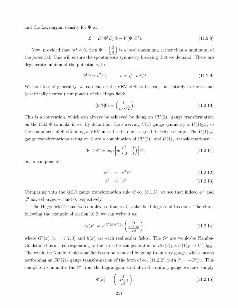
and the Lagrangian density for Φ is:

L = DµΦ†DµΦ− V (Φ,Φ†). (11.2.8)

Now, provided that m2 < 0, then Φ =(00

)is a local maximum, rather than a minimum, of

the potential. This will ensure the spontaneous symmetry breaking that we demand. There are

degenerate minima of the potential with

Φ†Φ = v2/2, v =√−m2/λ. (11.2.9)

Without loss of generality, we can choose the VEV of Φ to be real, and entirely in the second

(electrically neutral) component of the Higgs field:

〈0|Φ|0〉 =(

0v/√2

). (11.2.10)

This is a convention, which can always be achieved by doing an SU(2)L gauge transformation

on the field Φ to make it so. By definition, the surviving U(1) gauge symmetry is U(1)EM, so

the component of Φ obtaining a VEV must be the one assigned 0 electric charge. The U(1)EM

gauge transformations acting on Φ are a combination of SU(2)L and U(1)Y transformations:

Φ→ Φ′ = exp[iθ(1 00 0

)]Φ, (11.2.11)

or, in components,

φ+ → eiθφ+, (11.2.12)

φ0 → φ0. (11.2.13)

Comparing with the QED gauge transformation rule of eq. (8.1.5), we see that indeed φ+ and

φ0 have charges +1 and 0, respectively.

The Higgs field Φ has two complex, so four real, scalar field degrees of freedom. Therefore,

following the example of section 10.2, we can write it as:

Φ(x) = eiGa(x)σa/2v

(0

v+h(x)√2

), (11.2.14)

where Ga(x) (a = 1, 2, 3) and h(x) are each real scalar fields. The Ga are would-be Nambu-

Goldstone bosons, corresponding to the three broken generators in SU(2)L×U(1)Y → U(1)EM.

The would-be Nambu-Goldstone fields can be removed by going to unitary gauge, which means

performing an SU(2)L gauge transformation of the form of eq. (11.2.2), with θa = −Ga/v. This

completely eliminates the Ga from the Lagrangian, so that in the unitary gauge we have simply

Φ(x) =

(0

v+h(x)√2

). (11.2.15)

251

The field h creates and destroys the physical Higgs particle, an electrically neutral real scalar

boson that has yet to be discovered experimentally. We can now plug this into the Lagrangian

density of eq. (11.2.8), to find interactions and mass terms for the remaining Higgs field h and

the vector bosons. The covariant derivative of Φ in unitary gauge is:

DµΦ =1√2

(0∂µh

)+

i√2

[g′

2Bµ +

g

2W a

µσa

] (0

v + h

), (11.2.16)

and its Hermitian conjugate is:

DµΦ† =

1√2( 0 ∂µh )−

i√2( 0 v + h )

[g′

2Bµ +

g

2W a

µσa

]. (11.2.17)

Therefore,

DµΦ†DµΦ =1

2∂µh∂

µh+(v + h)2

8( 0 1 )

(g′Bµ + gW 3

µ

√2gW−

µ√2gW+

µ g′Bµ − gW 3µ

)

(g′Bµ + gW 3µ

√2gW−µ√

2gW+µ g′Bµ − gW 3µ

)(01

), (11.2.18)

or, after simplifying,

DµΦ†DµΦ =1

2∂µh∂

µh+(v + h)2

4

[g2W+

µ W−µ +

1

2(gW 3

µ − g′Bµ)(gW3µ − g′Bµ)

].(11.2.19)

This can be further simplified using:

gW 3µ − g′Bµ =

√g2 + g′2

[cos θWW

3µ − sin θWBµ

]=√g2 + g′2 Zµ, (11.2.20)

where the first equality uses eq. (11.1.30) and the second uses eq. (11.1.20). So finally we have:

LΦ kinetic = DµΦ†DµΦ =1

2∂µh∂

µh+(v + h)2

4

[g2W+

µ W−µ +

1

2(g2 + g′2)ZµZ

µ]. (11.2.21)

The parts of this proportional to v2 make up (mass)2 terms for the W± and Z vector bosons,

vindicating the earlier assumption of neutral vector boson mixing with the form that we took

for the sine and cosine of the weak mixing angle. Since there is no such (mass)2 term for the

photon field Aµ, we have successfully shown that the photon remains massless, in agreement

with the fact that U(1)EM gauge invariance remains unbroken. The specific prediction is:

m2W =

g2v2

4, m2

Z =(g2 + g′2)v2

4, (11.2.22)

which agrees with the experimental values provided that the VEV is approximately:

v =√2〈φ0〉 = 246 GeV (11.2.23)

252

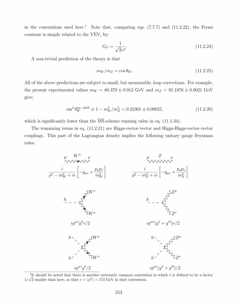
in the conventions used here.† Note that, comparing eqs. (7.7.7) and (11.2.22), the Fermi

constant is simply related to the VEV, by:

GF =1√2v2

. (11.2.24)

A non-trivial prediction of the theory is that

mW/mZ = cos θW . (11.2.25)

All of the above predictions are subject to small, but measurable, loop corrections. For example,

the present experimental values mW = 80.379 ± 0.012 GeV and mZ = 91.1876 ± 0.0021 GeV

give:

sin2 θon−shellW ≡ 1−m2

W/m2Z = 0.22301± 0.00025, (11.2.26)

which is significantly lower than the MS-scheme running value in eq. (11.1.34).

The remaining terms in eq. (11.2.21) are Higgs-vector-vector and Higgs-Higgs-vector-vector

couplings. This part of the Lagrangian density implies the following unitary gauge Feynman

rules:

i

p2 −m2W + iǫ

[−gµν +

pµpνm2

W

]

W±µ ν

i

p2 −m2Z + iǫ

[−gµν +

pµpνm2

Z

]

Zµ ν

igµνg2v/2

h

W ν

W µ

igµν(g2 + g′2)v/2

h

Zµ

Zν

igµνg2/2

h

h

W µ

W ν

igµν(g2 + g′2)/2

h

h

Zµ

Zν

†It should be noted that there is another extremely common convention in which v is defined to be a factor1/√2 smaller than here, so that v = 〈φ0〉 = 174 GeV in that convention.

253

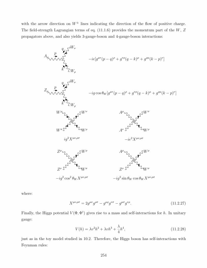
with the arrow direction on W± lines indicating the direction of the flow of positive charge.

The field-strength Lagrangian terms of eq. (11.1.6) provides the momentum part of the W , Z

propagators above, and also yields 3-gauge-boson and 4-gauge-boson interactions:

−ie[gµν(p− q)ρ + gνρ(q − k)µ + gρµ(k − p)ν ]

Wρ

Wν

Aµ

pq

k

−ig cos θW [gµν(p− q)ρ + gνρ(q − k)µ + gρµ(k − p)ν ]

Wρ

Wν

Zµ

pq

k

ig2Xµν,ρσ

W µ

W σ

W ν

W ρ

−ie2Xµν,ρσ

Aµ

Aν

W σ

W ρ

−ig2 cos2 θWXµν,ρσ

Zµ

Zν

W ρ

W σ

−ig2 sin θW cos θWXµν,ρσ

Aµ

Zν

W ρ

W σ

where:

Xµν,ρσ = 2gµνgρσ − gµρgνσ − gµσgνρ. (11.2.27)

Finally, the Higgs potential V (Φ,Φ†) gives rise to a mass and self-interactions for h. In unitary

gauge:

V (h) = λv2h2 + λvh3 +λ

4h4, (11.2.28)

just as in the toy model studied in 10.2. Therefore, the Higgs boson has self-interactions with

Feynman rules:

254

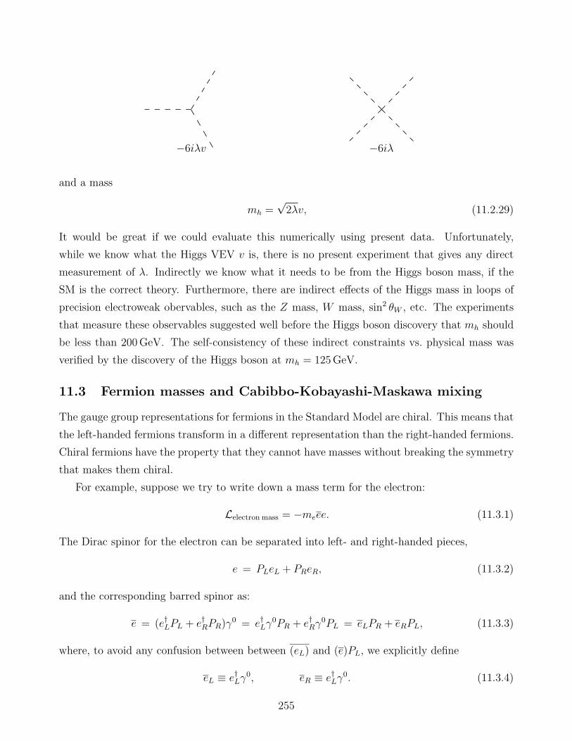
−6iλv −6iλ

and a mass

mh =√2λv, (11.2.29)

It would be great if we could evaluate this numerically using present data. Unfortunately,

while we know what the Higgs VEV v is, there is no present experiment that gives any direct

measurement of λ. Indirectly we know what it needs to be from the Higgs boson mass, if the

SM is the correct theory. Furthermore, there are indirect effects of the Higgs mass in loops of

precision electroweak obervables, such as the Z mass, W mass, sin2 θW , etc. The experiments

that measure these observables suggested well before the Higgs boson discovery that mh should

be less than 200GeV. The self-consistency of these indirect constraints vs. physical mass was

verified by the discovery of the Higgs boson at mh = 125GeV.

11.3 Fermion masses and Cabibbo-Kobayashi-Maskawa mixing

The gauge group representations for fermions in the Standard Model are chiral. This means that

the left-handed fermions transform in a different representation than the right-handed fermions.

Chiral fermions have the property that they cannot have masses without breaking the symmetry

that makes them chiral.

For example, suppose we try to write down a mass term for the electron:

Lelectron mass = −meee. (11.3.1)

The Dirac spinor for the electron can be separated into left- and right-handed pieces,

e = PLeL + PReR, (11.3.2)

and the corresponding barred spinor as:

e = (e†LPL + e†RPR)γ0 = e†Lγ

0PR + e†Rγ0PL = eLPR + eRPL, (11.3.3)

where, to avoid any confusion between between (eL) and (e)PL, we explicitly define

eL ≡ e†Lγ0, eR ≡ e†Lγ

0. (11.3.4)

255

Equation (11.3.1) can therefore be written:

Lelectron mass = −me(eLeR + eReL). (11.3.5)

The point is that this is clearly not a gauge singlet. In the first place, the eL part of each

term transforms as a doublet under SU(2)L, and the eR is a singlet, so each term is an SU(2)L

doublet. Furthermore, the first term has Y = YeR − YeL = −1/2, while the second term has

Y = 1/2. All terms in the Lagrangian must be gauge singlets in order not to violate the gauge

symmetry, so the electron mass is disqualified from appearing in this form. More generally, for

any Standard Model fermion f , the naive mass term

Lf mass = −mf (fLfR + fRfL) (11.3.6)

is not an SU(2)L singlet, and is not neutral under U(1)Y , and so is not allowed.

Fortunately, fermion masses can still arise with the help of the Higgs field. For the electron,

there is a gauge-invariant term:

Lelectron Yukawa = −ye ( νe eL )(φ+

φ0

)eR + c.c. (11.3.7)

Here ye is a Yukawa coupling of the type we studied in 6.3. The field ( νe eL ) carries weak

hypercharge +1/2, as does the Higgs field, and eR carries weak hypercharge −1, so the whole

term is a U(1)Y singlet, as required. Moreover, the doublets transform under SU(2)L as:

(φ+

φ0

)→ e−iθaσa/2

(φ+

φ0

), (11.3.8)

( νe eL ) → ( νe eL ) e+iθaσa/2, (11.3.9)

so eq. (11.3.7) is also an SU(2)L singlet. Going to the unitary gauge of eq. (11.2.15), it becomes:

LYukawa = −ye√2(v + h)(eLeR + eReL), (11.3.10)

or, reassembling the Dirac spinors without projection matrices:

LYukawa = −ye√2(v + h)ee. (11.3.11)

This can now be interpreted as an electron mass, equal to

me =yev√2, (11.3.12)

and, as a bonus, an electron-positron-Higgs interaction vertex, with Feynman rule:

256

−iye/√2

Since we know the electron mass and the Higgs VEV already, we can compute the electron

Yukawa coupling:

ye =√2(0.511 MeV

246 GeV

)= 2.94× 10−6. (11.3.13)

Unfortunately, this is so small that we can forget about ever observing the interactions of the

Higgs particle h with an electron. Notice that although the neutrino participates in the Yukawa

interaction, it disappears in unitary gauge from that term.

Masses for all of the other leptons, and the down-type quarks (d, s, b) in the Standard Model

arise in exactly the same way. For example, the bottom quark mass comes from the gauge-

invariant Yukawa coupling:

L = −yb ( tL bL )(φ+

φ0

)bR + c.c., (11.3.14)

implying that, in unitary gauge, we have a b-quark mass and an hbb vertex:

L = − yb√2(v + h)bb. (11.3.15)

The situation is slightly different for up-type quarks (u, c, t), because the complex conjugate of

the field Φ must appear in order to preserve U(1)Y invariance. It is convenient to define

Φ ≡(

0 1−1 0

)Φ∗ =

(φ0∗

−φ+∗

), (11.3.16)

which transforms as an SU(2)L doublet in exactly the same way that Φ does:

Φ → eiθaσa/2Φ, (11.3.17)

Φ → eiθaσa/2Φ. (11.3.18)

Also, Φ has weak hypercharge Y = −1/2. (The field φ+∗ has a negative electric charge.)

Therefore, one can write a gauge-invariant Yukawa coupling for the top quark as:

L = −yt ( tL bL )(φ0∗

−φ+∗

)tR + c.c. (11.3.19)

257

Going to unitary gauge, one finds that the top quark has a mass:

L = − yt√2(v + h)tt. (11.3.20)

In all cases, the unitary-gauge version of the gauge-invariant Yukawa interaction is

L = − yf√2(v + h)ff. (11.3.21)

The mass and the h-fermion-antifermion coupling obtained by each Standard Model fermion in

this way are both proportional to yf . The Higgs mechanism not only explains the masses of

the W± and Z bosons, but also explains the masses of fermions. Notice that all of the particles

in the Standard Model (except the photon and gluon, which must remain massless because of

SU(3)c×U(1)EM gauge invariance) get a mass from spontaneous electroweak symmetry breaking

of the form:

mparticle = kv, (11.3.22)

where k is some combination of dimensionless couplings. For the fermions, it is proportional to

a Yukawa coupling; for the W± and Z bosons it depends on gauge couplings, and for the Higgs

particle itself, it is the Higgs self-coupling λ.

There are two notable qualifications for quarks. First, gluon loops make a large modification

to the tree-level prediction. For each quark, the physical mass measured from kinematics is

mq =yqv√2

[1 +

4αs

3π+ . . .

], (11.3.23)

where yq is the running (renormalized) Yukawa coupling evaluated at a renormalization scale

µ = mq. The QCD gluon-loop correction increases mt by roughly 6%, and has an even larger

effect on mb because αs is larger at the renormalization scale µ = mb than at µ = mt. The

two-loop and higher corrections (indicated by . . .) are smaller but still significant, and must be

taken into account in precision work, for example when predicting the branching ratios of the

Higgs boson decay. This was the reason for the notation mf (more nearly yfv/√2 than mf )

that was used in 6.3.

A second qualification is that there is actually another source of quark masses, coming from

non-perturbative QCD effects, as has already been mentioned at the end of section 10.3. If

the Higgs field did not break SU(2)L × U(1)Y , then these chiral symmetry breaking effects

would do it anyway, using an antifermion-fermion VEV rather than a scalar VEV. This gives

contributions to all quark masses that are roughly of order ΛQCD. For the top, bottom, and even

charm quarks, this is relatively insignificant. However, for the up and down quarks, it is actually

the dominant effect. They get only a few MeV of their mass from the Higgs field. Therefore, the

258

most important source of mass in ordinary nuclear matter is really chiral symmetry breaking in

QCD, not the Standard Model Higgs field.

The Standard Model fermions consist of three families with identical gauge interactions.

Therefore, the most general form of the Yukawa interactions is actually:

Le,µ,τ Yukawas = −(νi ℓ

i

L

) (φ+

φ0

)yei

jℓRj + c.c., (11.3.24)

Ld,s,bYukawas = −(uiL d

i

L

)(φ+

φ0

)ydi

jdRj + c.c., (11.3.25)

Lu,c,tYukawas = −(uiL d

i

L

)( φ0∗

−φ+∗

)yui

juRj + c.c. (11.3.26)

Here i, j are indices that run over the three families, so that:

ℓRj =

eRµR

τR

, ℓLj =

eLµL

τL

, νi =

νeνµντ

, (11.3.27)

dLj =

dLsLbL

, dRj =

dRsRbR

, uLj =

uLcLtL

, uRj =

uRcRtR

. (11.3.28)

In a general basis, the Yukawa couplings

yeij, ydi

j, yuij (11.3.29)

are complex 3×3 matrices in family space. In unitary gauge, the Yukawa interaction Lagrangian

can be written as:

L = −(1 +

h

v

)ℓ′iLmei

jℓ′Rj + d′iLmdi

jd′Rj + u′iLmuiju′Rj

+ c.c., (11.3.30)

where

mf ij =

v√2yf i

j. (11.3.31)

(The fermion fields are now labeled with a prime, to distinguish them from the basis we are about

to introduce.) It therefore appears that the masses of Standard Model fermions are actually

3× 3 complex matrices.

Its is most convenient to work in a basis in which the fermion masses are real and positive,

so that the Feynman propagators are simple. This can always be accomplished, thanks to the

following:

Mass Diagonalization Theorem. Any complex matrix M can be diagonalized

by a biunitary transformation:

U †LMUR =MD (11.3.32)

whereMD is diagonal with positive real entries, and UL and UR are unitary matrices.

259

To apply this in the present case, consider the following redefinition of the lepton fields:

ℓ′Li = LLijℓLj, ℓ′Ri = LRi

jℓRj. (11.3.33)

where LLij and LRi

j are unitary 3 × 3 matrices. The lepton mass term in the unitary gauge

Lagrangian then becomes:

L = −(1 +

h

v

)ℓi

L(L†LmeLR)i

jℓRj. (11.3.34)

Now, the theorem just stated assures us that we can choose the matrices LL and LR so that:

L†LmeLR =

me 0 00 mµ 00 0 mτ

. (11.3.35)

So we can write in terms of the unprimed (mass eigenstate) fields:

L = −(1 +

h

v

)(meee+mµµµ+mτττ). (11.3.36)

In the same way, one can do unitary-matrix redefinitions of the quark fields:

d′Li = DLijdLj, d′Ri = DRi

jdRj, (11.3.37)

u′Li = ULijuLj, u′Ri = URi

juRj , (11.3.38)

chosen in such a way that

D†LmdDR =

md 0 00 ms 00 0 mb

, (11.3.39)

U †LmuUR =

mu 0 00 mc 00 0 mt

, (11.3.40)

with real and positive diagonal entries.

It might now seem that worrying about the possibility of non-diagonal 3×3 Yukawa matrices

was just a waste of time, but one must now consider how these field redefinitions from primed

(gauge eigenstate) to unprimed (mass eigenstate) fields affect the other terms in the Lagrangian.

First, consider the derivative kinetic terms. For the leptons, L contains

iℓj′L/∂ℓ′Lj = i(ℓLL

†L)

j /∂(LLℓL)j = iℓj

L/∂ℓLj. (11.3.41)

This relies on the fact that the (constant) field redefinition matrix LL is unitary, L†LLL = 1.

The same thing works for all of the other derivative kinetic terms, for example, for right-handed

up-type quarks:

iuj′R/∂u′Rj = i(uRU

†R)

j /∂(URuR)j = iujR/∂uRj, (11.3.42)

260

which relies on U †RUR = 1. So the redefinition has no effect at all here; the form of the derivative

kinetic terms is exactly the same for unprimed fields as for primed fields.

There are also interactions of fermions with gauge bosons. For example, for the right-handed

leptons, the QED Lagrangian contains a term

−eAµℓj′Rγ

µℓ′Rj = −eAµ(ℓRL†R)

jγµ(LRℓR)j = −eAµℓj

RγµℓRj. (11.3.43)

Just as before, the unitary condition (this time L†RLR = 1) guarantees that the form of the

Lagrangian term is exactly the same for unprimed fields as for primed fields. You can show

quite easily that the same thing applies to interactions of all fermions with Zµ and the gluon

fields. The unitary redefinition matrices for quarks just commute with the SU(3)c generators,

since they act on different indices.

But, there is one place in the Standard Model where the above argument does not work,

namely the interactions of W± vector bosons. This is because the W± interactions involve

two different types of fermions, with different unitary redefinition matrices. Consider first the

interactions of the W± with leptons. In terms of the original primed fields:

L = − g√2W+

µ ν′iγµℓ′Li + c.c., (11.3.44)

so that

L = − g√2W+

µ ν′iγµ(LLℓL)i + c.c. (11.3.45)

Since we did not include a Yukawa coupling or mass term for the neutrinos, we did not have to

make a unitary redefinition for them. But now we are free to do so; defining νi in the same way

as the corresponding charged leptons, ν ′i = LLνj, we get,

ν ′i = (νL†L)

i, (11.3.46)

resulting in

L = − g√2W+

µ νiγµℓLi + c.c. (11.3.47)

So once again the interactions of W± bosons have exactly the same form for mass-eigenstate

leptons. However, consider the interactions of W± bosons with quarks. In terms of the original

primed fields,

L = − g√2W+

µ u′iLγ

µd′Li + c.c., (11.3.48)

which becomes:

L = − g√2W+

µ uiLγ

µ(U †LDLdL)i + c.c. (11.3.49)

261

There is no reason why U †LDL should be equal to the unit matrix, and in fact it is not. So we have

finally encountered a consequence of going to the mass-eigenstate basis. The charged-current

weak interactions contain a non-trivial matrix operating in quark family space,

V = U †LDL, (11.3.50)

called the Cabibbo-Kobayashi-Maskawa matrix (or CKM matrix). The CKM matrix V is itself

unitary, since V † = (U †LDL)

† = D†LUL, implying that V †V = V V † = 1. But, it cannot be

removed by going to some other basis using a further unitary matrix without ruining the diagonal

quark masses. So we are stuck with it.

One can think of V as just a unitary rotation acting on the left-handed down quarks. From

eq. (11.3.49), we can define

d′Li = VijdLj, (11.3.51)

where the dLj are mass eigenstate quark fields, and the d′Li are the quarks that interact in a

simple way with W bosons:

L = − g√2W+

µ uiLγ

µd′Li + c.c., (11.3.52)

and so in terms of mass eigenstate quark fields:

L = − g√2Vi

j W+µ u

iLγ

µdLj + c.c. (11.3.53)

This is the entire effect of the non-diagonal Yukawa matrices.

The numerical entries of the CKM matrix are a subject of continuing experimental investi-

gation. To a first approximation, it turns out that the CKM mixing is just a rotation of down

and strange quarks:

V =

cos θc sin θc 0− sin θc cos θc 0

0 0 1

(11.3.54)

where θc is called the Cabibbo angle. This implies that the interactions of W+ with the mass-

eigenstate quarks are very nearly:

L = − g√2W+

µ

(cos θc[uLγ

µdL + cLγµsL] + sin θc[uLγ

µsL − cLγµdL] + tLγµbL

). (11.3.55)

The terms proportional to sin θc are responsible for strangeness-changing decays. Numerically,

cos θc ≈ 0.974, sin θc ≈ 0.23. (11.3.56)

262

Strange hadrons have long lifetimes because they decay through the weak interactions, and with

reduced matrix elements that are proportional to sin2 θc = 0.05.

More precisely, the CKM matrix is:

V =

Vud Vus VubVcd Vcs VcbVtd Vts Vtb

≈

0.9743 0.2252 0.0040.230 0.975 0.0410.008 0.04 0.999

, (11.3.57)

where the numerical values given are estimates of the magnitude only (not the sign or phase).

In fact, the CKM matrix contains one phase that cannot be removed by redefining phases of

the fermion fields. This phase is the only source of CP violation in the Standard Model.

Weak decays of mesons involving the W bosons allow the entries of the CKM matrix to be

probed experimentally. For example, decays

B → Dℓ+νℓ, (11.3.58)

where B is a meson containing a bottom quark and D contains a charm quark, can be used to

extract |Vcb|. The very long lifetimes of B mesons are explained by the fact that |Vub| and |Vcb|are very small. One of the ways of testing the Standard Model is to check that the CKM matrix

is indeed unitary:

V †V = 1, (11.3.59)

which implies in particular that VudV∗ub+VcdV

∗cb+VtdV

∗tb = 0. This is an automatic consequence of

the Standard Model, but if there is further unknown physics out there, then the weak interactions

could appear to violate CKM unitarity.

The partial decay widths and branching ratios of the W boson can be worked out from

eqs. (11.3.47) and (11.3.53), and agree well with the experimental results:

BR(W+ → ℓ+νℓ) = 0.1086± 0.0009 (for ℓ = e, µ, τ , each) (11.3.60)

BR(W+ → hadrons) = 0.6741± 0.0027. (11.3.61)

where the “hadrons” refers mostly to Cabibbo-allowed final states ud and cs, with a much

smaller contribution from the Cabibbo-suppressed final states cd and us. The tb final state is

of course not available due to kinematics; this implies the useful fact that (up to a very small

effect from CKM mixing) b quarks do not result from W decays in the Standard Model.

Also, the very small magnitudes of Vtd and Vts imply that top quarks decay to bottom quarks

almost every time:

BR(t→ W+b) ≈ 1. (11.3.62)

This greatly simplifies the experimental identification of top quarks.

263

11.4 Neutrino masses and the seesaw mechanism

Evidence from observation of neutrinos produced in the Sun, the atmosphere, accelerators, and

reactors have now established that neutrinos do have mass. In the renormalizable version of the

Standard Model given up to here, this cannot be explained. The basic reason for this is the

absence of right-handed neutrinos from the list in eq. (11.1.35). To remedy the situation, we

can add three right-handed fermions that are singlets under all three components of the gauge

group SU(3)c × SU(2)L × U(1)Y :

NR1, NR2, NR3 ←→ (1, 1, 0). (11.4.1)

With these additional gauge-singlet right-handed neutrino degrees of freedom, it is now possible

to write down a gauge-invariant Lagrangian interaction of the neutrinos with the Higgs field:

Lν neutrino Yukawas = −(νi ℓ

i

L

) ( φ0∗

−φ+∗

)yνi

jNRj + c.c. (11.4.2)

Note the similarity of this with the up-type quark Yukawa couplings in eq. (11.3.26). Going to

unitary gauge, one obtains a neutrino mass matrix

mνij =

v√2yνi

j. (11.4.3)

just as in eq. (11.3.31) for the Standard Model charged fermions. This neutrino mass matrix can

be diagonalized to obtain the physical neutrino masses as the absolute values of its eigenvalues.

The neutrinos in this scenario are Dirac fermions, as the mass term couples together left-handed

and right-handed degrees of freedom that are independent.

Although the magnitudes of the neutrino masses are not yet determined by experiment, there

are strong upper bounds, as seen in Table 1.2 in the Introduction. Also, limits from the WMAP

and Planck measurements of the cosmic background radiation, interpreted within the standard

cosmological model, implies that the sum of the three Standard Model neutrinos should be at

most 0.17 eV. Neutrino oscillation data do not constrain the individual neutrino masses, but

imply that the largest differences between squared masses should be less than 3 × 10−3 eV2.

So, several independent pieces of evidence indicate that neutrino masses are much smaller that

any of the charged fermion masses. To accommodate this within the Dirac mass framework of

eq. (11.4.3), the eigenvalues of the neutrino Yukawa matrix yνij would have to be extremely

small, no larger than about 10−9. Such small dimensionless couplings appear slightly unnatural,

in a purely subjective sense, and this suggests that neutrino masses may have a different origin

than quark and leptons masses.

The seesaw mechanism is a way of addressing this problem, such that very small neutrino

masses naturally occur, even if the corresponding Yukawa couplings are of order 1. One includes,

264

besides eq. (11.4.2), a new term in the Lagrangian:

L = −1

2MijN iNj, (11.4.4)

where Ni are the Majorana fermion fields (see section 3.4) that include NRi, and Mij is a

symmetric mass matrix. If the neutrino fields carry lepton number 1, then this Majorana mass

term necessarily violates the total lepton number L = Le+Lµ+Lτ . Now the total mass matrix

for the left-handed neutrino fields νLi and the right-handed neutrino fields NRi, including both

eq. (11.4.3) and eq. (11.4.4), is:

M =

(0 v√

2yν

v√2yTν M

). (11.4.5)

The point of the seesaw mechanism is that if the eigenvalues of M are much larger than those

of the Dirac mass matrix v√2yν , then the smaller set of mass eigenvalues of M will be pushed

down. Since M does not arise from electroweak symmetry breaking, it can naturally be very

large. For illustration, taking M and yν to be 1×1 matrices, the absolute values of the neutrino

mass eigenvalues ofM are approximately:

v2yν2

2M, and M (11.4.6)

in the limit vyν ≪ M. For example, to get a neutrino mass of order 0.1 eV, one could have

yν = 1.0 and M = 3 × 1014 GeV, or yν = 0.1 and M = 3 × 1012 GeV. The light neutrino

states (corresponding to the lighter eigenvectors of M) are mostly the Standard Model νL

and they are Majorana fermions. There are also three extremely heavy Majorana neutrino

mass eigenstates, which decouple from present weak interaction experiments. The fact that the

magnitude of M necessary to make this work is not larger than the Planck scale, and is very

roughly commensurate with other scales that occur in other theories such as supersymmetry, is

encouraging. In any case, the ease with which the seesaw mechanism accommodates very small

but non-zero neutrino masses has made it a favorite scenario of theorists.

In either of the two cases above, the left-handed parts of the neutrino mass eigenstates

ν1, ν2, ν3 (with masses m1 < m2 < m3) can be related to the left-handed parts of the neutrino

weak-interaction eigenstates νe, νµ, ντ (which each couple to the corresponding charged lepton

only, and the W boson) by:νeLνµLντL

= U

ν1Lν2Lν3L

, (11.4.7)

where U is a unitary matrix known as the Pontecorvo-Maki-Nakagawa-Sakata (PMNS) matrix.

Neutrino oscillations are due to the fact that U is not equal to the identity matrix.

265

To recap, by introducing right-handed gauge-singlet neutrino decrees of freedom, there are

two distinct scenarios for neutrino masses. In the Dirac scenario, neutrinos and antineutrinos

are distinct, and total lepton number is conserved although the individual lepton numbers are

violated. In the Majorana scenario, neutrinos are their own antiparticles, and total lepton

number is violated along with the individual lepton numbers. At this writing, both possibilities

are consistent with the experimental data. To tell the difference between these two scenarios,

one can look for neutrinoless double beta decay, i.e. a nuclear transition

AZ → A(Z + 2) + e−e−, (11.4.8)

(at the nucleon level nn → ppe−e−), which can proceed via the quark-level Feynman diagram

shown below.

e−

e−

u

u

d

d

ν

W−

W−

Since this process requires a violation of total lepton number in the neutrino propagator, it can

only occur in the case of Majorana neutrinos. It is the subject of continuing searches.

11.5 The Higgs boson discovery

One of the most momentous discoveries of the last half century was that of the Higgs boson.

Before its discovery in 2012, its properties and even its existence were in doubt, despite the many

successes of the Standard Model. Research publications on “Higgsless theories” had persisted to

the very end. As discussed above, the simplest path to achieve masses for the W and Z bosons

and the fermions of the Standard Model is to introduce a single scalar Higgs boson doublet

that condenses, breaking electroweak symmetry down to the U(1)EM. The fluctuation around

this background value is the Higgs boson. However, when the theory was first formulated,

there was little guidance as to what mass it should have. One only knew that it was controlled

by the vacuum expectation value, which was known to be v ≃ 246GeV, and a dimensionless

constant λ that was completely unknown, leading to an unknown mass mh =√2λv, as we saw

in eq. (11.2.29).

Experiments had been searching for the Higgs boson for decades without success. Just prior

to its discovery, evidence from the sum of data collected from the Z pole experiments at CERN

LEP and SLAC SLC, combined with the top quark and W mass measurements at Tevatron

266

and LEP2 at CERN, suggested that if the Standard Model is the underlying theory of the weak

scale, then the Higgs boson mass needed to be in the range 114GeV < mh<∼ 180GeV at 95%

confidence level. It should be emphasized that the lower bound of 114GeV was derived directly

by not seeing the Higgs boson produced and decay at LEP2, whereas the upper bound was

derived indirectly, and thus less reliably, by a global analysis of compatibility to all data that

is sensitive to the Higgs boson mass, via quantum loops. A problem with this kind of indirect

bound is that it is always possible that some other unsuspected particle(s) also contribute in

the loops, interfering with the Higgs boson contribution.

Below, we will review the physics of the Higgs boson discovery at the LHC, starting with a

discussion of the decay modes.

11.5.1 Higgs boson decays revisited

In section 6.3, we have already calculated the leading-order decays of the Higgs boson into

fermion-antifermion final states. However, there are other final states that are quite important

besides h → ff . First, the Higgs boson can decay into two gluons, h → gg, with the gluons

eventually manifesting themselves in the detector as jets. This decay cannot happen at tree

level, but does occur through the one-loop diagram below, where quarks go around the loop:

h

g

g

q

q

q

(One must also include the diagram with the gluons exchanged, or equivalently the diagram

with the quarks running the other direction around the loop.) Even though one-loop graph

amplitudes are usually not competitive with tree-level amplitudes, this is an exception because

the gluons have strong couplings and because the top quark with its large yt participates in the

loop diagrams, while in the on-shell 2-body decays to fermions, only lighter fermions (with much

smaller Yukawa couplings) can appear.

The resulting partial decay width for h → gg depends on the quark masses in two places.

First, at the hqq vertex there is a Yukawa coupling, and second there needs to be a chirality

flip in one of the propagators to enable a non-zero result. That is, the trace over the three

fermion propagator numerators vanishes (due to an odd number of γ matrices) unless one of the

propagators is traced over the mass term. These two facts explain why the top quark, being by

far the most massive quark, gives a dominant contribution to this amplitude.

267

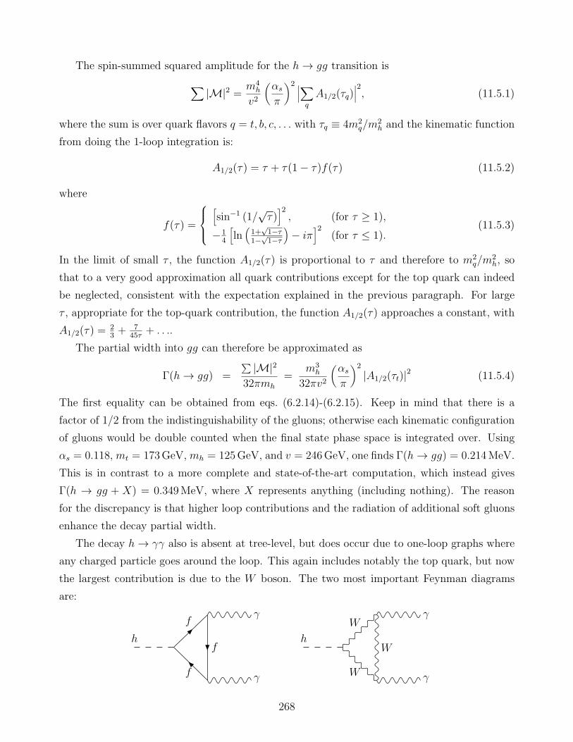
The spin-summed squared amplitude for the h→ gg transition is

∑|M|2 = m4

h

v2

(αs

π

)2 ∣∣∣∑

q

A1/2(τq)∣∣∣2, (11.5.1)

where the sum is over quark flavors q = t, b, c, . . . with τq ≡ 4m2q/m

2h and the kinematic function

from doing the 1-loop integration is:

A1/2(τ) = τ + τ(1− τ)f(τ) (11.5.2)

where

f(τ) =

[sin−1 (1/

√τ)]2, (for τ ≥ 1),

−14

[ln(1+

√1−τ

1−√1−τ

)− iπ

]2(for τ ≤ 1).

(11.5.3)

In the limit of small τ , the function A1/2(τ) is proportional to τ and therefore to m2q/m

2h, so

that to a very good approximation all quark contributions except for the top quark can indeed

be neglected, consistent with the expectation explained in the previous paragraph. For large

τ , appropriate for the top-quark contribution, the function A1/2(τ) approaches a constant, with

A1/2(τ) =23+ 7

45τ+ . . ..

The partial width into gg can therefore be approximated as

Γ(h→ gg) =

∑ |M|232πmh

=m3

h

32πv2

(αs

π

)2

|A1/2(τt)|2 (11.5.4)

The first equality can be obtained from eqs. (6.2.14)-(6.2.15). Keep in mind that there is a

factor of 1/2 from the indistinguishability of the gluons; otherwise each kinematic configuration

of gluons would be double counted when the final state phase space is integrated over. Using

αs = 0.118,mt = 173GeV,mh = 125GeV, and v = 246GeV, one finds Γ(h→ gg) = 0.214MeV.

This is in contrast to a more complete and state-of-the-art computation, which instead gives

Γ(h → gg + X) = 0.349MeV, where X represents anything (including nothing). The reason

for the discrepancy is that higher loop contributions and the radiation of additional soft gluons

enhance the decay partial width.

The decay h→ γγ also is absent at tree-level, but does occur due to one-loop graphs where

any charged particle goes around the loop. This again includes notably the top quark, but now

the largest contribution is due to the W boson. The two most important Feynman diagrams

are:

h

γ

γ

f

f

fh

γ

γ

W

W

W

268

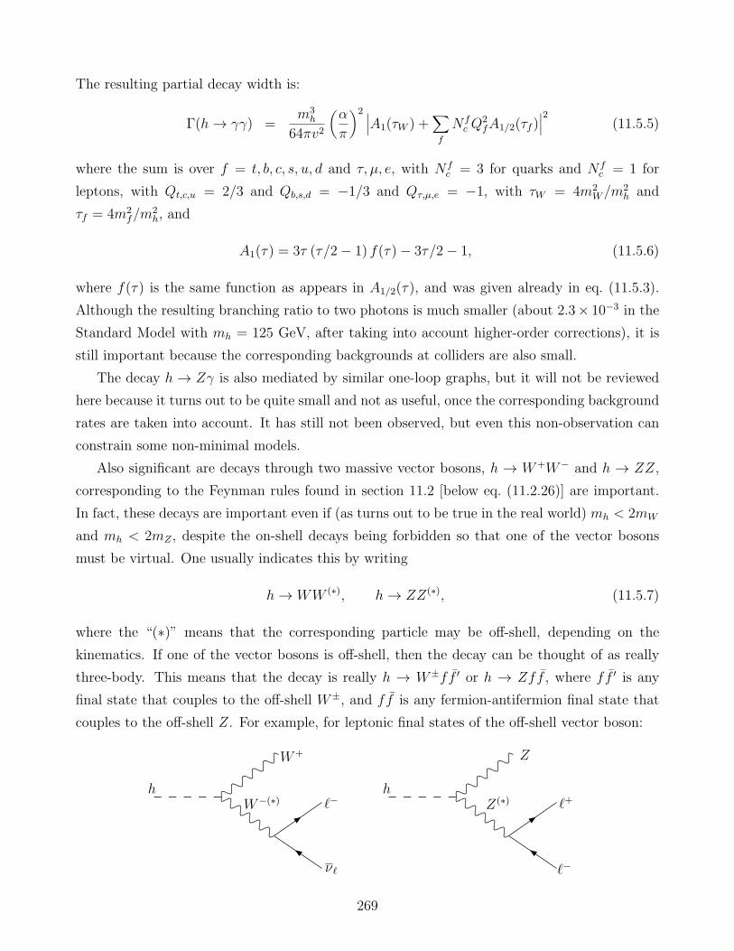
The resulting partial decay width is:

Γ(h→ γγ) =m3

h

64πv2

(α

π

)2 ∣∣∣A1(τW ) +∑

f

N fc Q

2fA1/2(τf )

∣∣∣2

(11.5.5)

where the sum is over f = t, b, c, s, u, d and τ, µ, e, with N fc = 3 for quarks and N f

c = 1 for

leptons, with Qt,c,u = 2/3 and Qb,s,d = −1/3 and Qτ,µ,e = −1, with τW = 4m2W/m

2h and

τf = 4m2f/m

2h, and

A1(τ) = 3τ (τ/2− 1) f(τ)− 3τ/2− 1, (11.5.6)

where f(τ) is the same function as appears in A1/2(τ), and was given already in eq. (11.5.3).

Although the resulting branching ratio to two photons is much smaller (about 2.3× 10−3 in the

Standard Model with mh = 125 GeV, after taking into account higher-order corrections), it is

still important because the corresponding backgrounds at colliders are also small.

The decay h→ Zγ is also mediated by similar one-loop graphs, but it will not be reviewed

here because it turns out to be quite small and not as useful, once the corresponding background

rates are taken into account. It has still not been observed, but even this non-observation can

constrain some non-minimal models.

Also significant are decays through two massive vector bosons, h → W+W− and h → ZZ,

corresponding to the Feynman rules found in section 11.2 [below eq. (11.2.26)] are important.

In fact, these decays are important even if (as turns out to be true in the real world) mh < 2mW

and mh < 2mZ , despite the on-shell decays being forbidden so that one of the vector bosons

must be virtual. One usually indicates this by writing

h→ WW (∗), h→ ZZ(∗), (11.5.7)

where the “(∗)” means that the corresponding particle may be off-shell, depending on the

kinematics. If one of the vector bosons is off-shell, then the decay can be thought of as really

three-body. This means that the decay is really h → W±ff ′ or h → Zff , where ff ′ is any

final state that couples to the off-shell W±, and ff is any fermion-antifermion final state that

couples to the off-shell Z. For example, for leptonic final states of the off-shell vector boson:

h

W+

W−(∗) ℓ−

νℓ

h

Z

Z(∗) ℓ+

ℓ−

269

Since the competing tree-level two-body decays h → ff are suppressed by small Yukawa cou-

plings, these three-body decays are competitive, despite their kinematic suppression. If we take

mh to be a free variable, as it was before the discovery, then the closer the vector bosons are to

being on-shell, the larger the amplitude will be. The decays h → WW (∗) become increasingly

important for larger mh, and would actually dominate if mh>∼ 135 GeV.

The results of a careful computation (using the program HDECAY by A. Djouadi, J. Kali-

nowski, and M. Spira, Comput. Phys. Commun. 108, 56, (1998), hep-ph/9704448) including all

these effects are shown in the two graphs below, which depict the state-of-the-art computations

of the branching ratios and the total width Γtot for the Higgs boson, as a function of mh for the

range allowed before the discovery in 2012.

100 120 140 160 180 200 220 240Higgs mass [GeV]

10-3

10-2

10-1

100

Hig

gs B

ranchin

g R

atio

bb

τ+τ−

cc

gg

W+W

−

ZZ

γγ

100 120 140 160 180 200 220 240Higgs mass [GeV]

10-3

10-2

10-1

100

Hig

gs T

ota

l W

idth

[G

eV

]

270

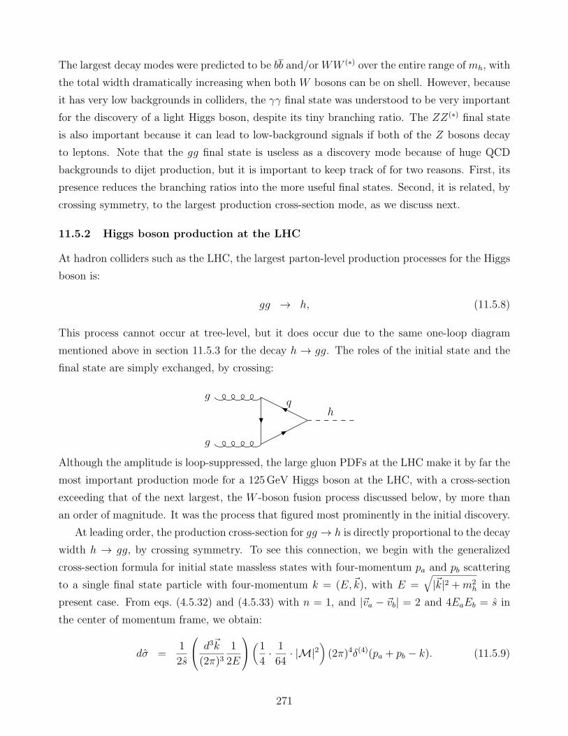
The largest decay modes were predicted to be bb and/orWW (∗) over the entire range ofmh, with

the total width dramatically increasing when both W bosons can be on shell. However, because

it has very low backgrounds in colliders, the γγ final state was understood to be very important

for the discovery of a light Higgs boson, despite its tiny branching ratio. The ZZ(∗) final state

is also important because it can lead to low-background signals if both of the Z bosons decay

to leptons. Note that the gg final state is useless as a discovery mode because of huge QCD

backgrounds to dijet production, but it is important to keep track of for two reasons. First, its

presence reduces the branching ratios into the more useful final states. Second, it is related, by

crossing symmetry, to the largest production cross-section mode, as we discuss next.

11.5.2 Higgs boson production at the LHC

At hadron colliders such as the LHC, the largest parton-level production processes for the Higgs

boson is:

gg → h, (11.5.8)

This process cannot occur at tree-level, but it does occur due to the same one-loop diagram

mentioned above in section 11.5.3 for the decay h → gg. The roles of the initial state and the

final state are simply exchanged, by crossing:

hq

g

g

Although the amplitude is loop-suppressed, the large gluon PDFs at the LHC make it by far the

most important production mode for a 125GeV Higgs boson at the LHC, with a cross-section

exceeding that of the next largest, the W -boson fusion process discussed below, by more than

an order of magnitude. It was the process that figured most prominently in the initial discovery.

At leading order, the production cross-section for gg → h is directly proportional to the decay

width h → gg, by crossing symmetry. To see this connection, we begin with the generalized

cross-section formula for initial state massless states with four-momentum pa and pb scattering

to a single final state particle with four-momentum k = (E,~k), with E =√|~k|2 +m2

h in the

present case. From eqs. (4.5.32) and (4.5.33) with n = 1, and |~va − ~vb| = 2 and 4EaEb = s in

the center of momentum frame, we obtain:

dσ =1

2s

d3~k

(2π)31

2E

(1

4· 164· |M|2

)(2π)4δ(4)(pa + pb − k). (11.5.9)

271

By crossing symmetry,∑ |M|2 is the same spin-summed and color-summed squared matrix

element as in the decay calculation, but here it comes with the prefactor 14· 164, since in this case

we need to average (instead of sum) over initial state gluon spins (2 spins) and color factors (8

gluons ga=1...8). Since the cross-section is invariant under boosts along the beam direction we

chose to work in the center-of-momentum frame where ~pa + ~pb = 0, so that the delta function

vanishes except for ~k = 0. For on-shell production of the Higgs boson, E =√s = mh.

Integrating Eq. (11.5.9) over the three-momentum ~k and collecting terms we find that

σ =π

256m2h

δ(s−m2h)∑|M|2 (11.5.10)

Now, from eq. (11.5.4) we know that∑ |M|2 = 32πmhΓ and so the cross-section of gg → h can

be obtained by knowing the partial decay width h→ gg:

σ(gg → h) =π2

8mh

Γ(h→ gg)δ(s−m2h). (11.5.11)

The δ function dependence of the cross-section corresponds to the fact that free, on-shell asymp-

totic states cannot scatter 2-to-1 unless the four-momenta of the first two particles pµa,b are pre-

cisely arranged to construct the final momentum k = p1 + p2 such that k2 = m2h. Unlike 2-to-2

scattering not just any sufficiently large incoming momenta will do. In the center of mass frame

this requires that E = mh and ~k = 0.

More generally, there is no way to allow AB → C particle scattering unless mA+mB ≤ mC .

However, if that is allowed, then C → AB decays are allowed with the same amplitude, giving

C a decay width. The decay width means that there is a finite spread of k2 around m2C (with

the finite spread being determined by ΓC) such that AB → C is allowed. The finite spread is

the Breit-Wigner width, which is characterized by replacing the δ-function with

δ(s−m2h) →

1

π

mhΓh

(s−m2h)

2 +m2hΓ

2h

. (11.5.12)

This is the correct physical and non-singular interpretation of the δ-function in Eq. (11.5.10),

as one can show by treating the Higgs boson as a virtual intermediate state with a Feynman

propagator. In practice, if the width is much less than the mass Γh ≪ mh, which is certainly

the case for the Standard Model Higgs boson at 125 GeV (for which the total width is Γh = 4.2

MeV, so Γh/mh ≃ 3.4×10−5), then the δ function is a good approximation. In general, replacing

the Breit-Wigner peak with a δ-function is called the “narrow width approximation.”

In our case the narrow width approximation is useful and appropriate because we need to

integrate over gluon-gluon luminosity in the very close neighborhood of√sgg = mh, and the

integrand hardly varies over the narrow width of the Higgs Breit-Wigner function. Writing g(x)

for the pdf of gluons at momentum fraction x, the total cross section in pp collisions is

σ(pp→ h) =∫ 1

0dxa

∫ 1

0dxb g(xa)g(xb)σ(gg → h) (11.5.13)

272

Recall that the partonic center of mass energy is s = xaxbs. It is convenient to define a different

set of variables,

τ = xaxb and x = xa. (11.5.14)

The Jacobian of this variable change is J = 1/x, so that

σ(pp→ h) =∫ 1

0dτ∫ 1

τ

dx

xg(x)g(τ/x)σ(τs). (11.5.15)

With these integration variables, the parton-level cross-section σ is a function of s = τs only,

and not x, so we can perform the x integral over the gluon PDFs separately. It is convenient to

define a function of τ only, called the gluon-gluon luminosity function:

dL(τ)dτ

=∫ 1

τ

dx

xg(x)g(τ/x), (11.5.16)

This leaves us with

σ(pp→ h) =∫ 1

0dτdL(τ)dτ

σ(τs). (11.5.17)

For a given fixed value of mh, the total leading-order cross-section for pp→ h due to the gg → h

parton-level process is therefore a simple function of s and mh, and can be obtained by using

the δ-function in σ to integrate over τ , with the result:

σ(pp→ h) = Fgg(τh)σ0 (11.5.18)

where

σ0 =π2

8m3h

Γ(h→ gg), (11.5.19)

and

Fgg(τh) = τh

∫ 1

τh

dx

xg(x)g(τh/x) (11.5.20)

is simply a dimensionless number dependent only on the ratio

τh = m2h/s, (11.5.21)

which in turn depends on the Higgs boson mass and the proton beam energy.

The numerical value of σ0, using the leading-order width Γ(h→ gg) = 0.214 MeV obtained

above, is:

σ0 =π2

8m3H

Γ(H → gg) ≃ 53 fb (11.5.22)

273

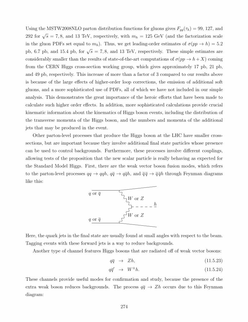
Using the MSTW2008NLO parton distribution functions for gluons gives Fgg(τh) = 99, 127, and

292 for√s = 7, 8, and 13 TeV, respectively, with mh = 125 GeV (and the factorization scale

in the gluon PDFs set equal to mh). Thus, we get leading-order estimates of σ(pp → h) = 5.2

pb, 6.7 pb, and 15.4 pb, for√s = 7, 8, and 13 TeV, respectively. These simple estimates are

considerably smaller than the results of state-of-the-art computations of σ(pp→ h+X) coming

from the CERN Higgs cross-section working group, which gives approximately 17 pb, 21 pb,

and 49 pb, respectively. This increase of more than a factor of 3 compared to our results above

is because of the large effects of higher-order loop corrections, the emission of additional soft

gluons, and a more sophisticated use of PDFs, all of which we have not included in our simple

analysis. This demonstrates the great importance of the heroic efforts that have been made to

calculate such higher order effects. In addition, more sophisticated calculations provide crucial

kinematic information about the kinematics of Higgs boson events, including the distribution of

the transverse momenta of the Higgs boson, and the numbers and momenta of the additional

jets that may be produced in the event.

Other parton-level processes that produce the Higgs boson at the LHC have smaller cross-

sections, but are important because they involve additional final state particles whose presence

can be used to control backgrounds. Furthermore, these processes involve different couplings,

allowing tests of the proposition that the new scalar particle is really behaving as expected for

the Standard Model Higgs. First, there are the weak vector boson fusion modes, which refers

to the parton-level processes qq → qqh, qq → qqh, and q q → q qh through Feynman diagrams

like this:

q or q

q or q

W or Z

W or Z

h

Here, the quark jets in the final state are usually found at small angles with respect to the beam.

Tagging events with these forward jets is a way to reduce backgrounds.

Another type of channel features Higgs bosons that are radiated off of weak vector bosons:

qq → Zh, (11.5.23)

qq′ → W±h. (11.5.24)

These channels provide useful modes for confirmation and study, because the presence of the

extra weak boson reduces backgrounds. The process qq → Zh occurs due to this Feynman

diagram:

274

q

q

h

Z

Z

while the process qq′ → W±h is due to parton-level Feynman diagrams like the ones below:

u

d

h

W+

W+

d

u

h

W−

W−

as well as others related by d→ s and/or u→ c.

Another important process, long anticipated but only very recently observed, is pp → tth,

which is due to Feynman diagrams including the one below:

g

g

t

t

h

This is particularly useful as a direct test of the Higgs boson interaction with the top quark.

11.5.3 The Higgs boson discovery

The pp Large Hadron Collider experiments at CERN, ATLAS and CMS, were both designed

to be able to cover the entire range of Higgs boson mass suggested by the indirect constraints

on it. For much of the allowed mass region, the primary target for discovery was the decay

to γγ, manifested as a narrow mass peak of two photons centered on mh = msignalγγ . The main

background, largely created by qq → γγ, consists of a diffuse spectrum of mbkgdγγ . There are also

important contributions to the background from gg → γγ and from fake photons.

Indeed, the diphoton signal is half of how the Higgs boson discovery was established – a peak

of γγ events that ultimately could be identified with mh. The left panel of Fig. 11.1 shows an

ATLAS collaboration plot of this γγ peak after data collection at√s = 7TeV and 8TeV. A

similar result was obtained by CMS.

The other half of the Higgs discovery came about via h → ZZ(∗) → 4ℓ decays of the Higgs

boson, where the (∗) indicates an off-shell Z boson, and 4ℓ indicates any one of the following

275

[GeV]γγm

110 120 130 140 150 160

weig

hts

- fitte

d b

kg

∑

-5

0

5

10

weig

hts

/ G

eV

∑

0

20

40

60

80

100

120

140

160

180

Data

Signal+background

Background

Signal

= 7 TeVs, -1dt = 4.5 fb L∫ = 8 TeVs, -1dt = 20.3 fb L∫

S/B weighted sum

Signal strength categories

= 125.4 GeVH

m

ATLAS

(GeV)l4m

80 100 120 140 160 180

Eve

nts

/ 3

Ge

V

0

5

10

15

20

25

30

35 Data

Z+X

,ZZ*γZ

=126 GeVHm

CMS-1

= 8 TeV, L = 19.7 fbs ; -1

= 7 TeV, L = 5.1 fbs

Figure 11.1: Left panel: The diphoton invariant mass spectrum from ATLAS data (Aad,G. et al. 2014 [ATLAS Collaboration], “Measurement of Higgs production in the diphotondecay channel in pp collisions at center-of-mass energies of 7 and 8 TeV with the ATLASdetector”, arXiv:1408.7084.). The upper red line is signal (from h→ γγ) plus background(mostly qq → γγ). The dashed blue line is a fit to the background-only hypothesis. Theblack curves on the bottom show the signal expectation (black solid curve) and the back-ground subtracted data (data circles with 68% CL vertical uncertainty bars). Right panel:The four-lepton invariant mass spectrum from CMS (Chatrchyan, S. et al. 2014 [CMS Col-laboration], “Measurement of the properties of a Higgs boson in the four-lepton final state”,arXiv:1312.5353.) is shown as the black data points. The prediction from backgroundsother than the Standard Model Higgs boson are shown as the blue histogram. The redcurve includes the backgrounds plus the prediction of a Higgs boson with invariant masspeak of mh = m4l = 125GeV.

permutations: e+e−e+e−, µ+µ−µ+µ− or e+e−µ+µ−. This branching fraction is very small. From

eqs. (6.3.29) and (11.1.43) above, we have:

BR(h→ ZZ(∗) → 4l) = BR(h→ ZZ(∗))[BR(Z → e+e−) + BR(Z → µ+µ−)]2 (11.5.25)

≈ 0.0264(0.067316)2 ≈ 0.000120. (11.5.26)

Fortunately, the backgrounds for four leptons near an invariant mass of m4ℓ = mh are also very

small. This enables a signal to be discerned above the background. This is illustrated in the

right panel of Fig. 11.1, which shows a plot of the invariant mass distribution of four lepton final

states recorded by the CMS collaboration in the√s = 7TeV and 8TeV runs. Again, a similar

result was obtained by ATLAS. The consistency of the diphoton and ZZ(∗) → 4ℓ invariant mass

peaks in the ATLAS and CMS experiments then allowed a definitive discovery.

276

The announced discovery of the Higgs boson in July 2012 has given rise to a new era in

particle physics phenomenology. The present and future research efforts of the LHC will be

centered around careful measurements of the Higgs boson, as well as the search for any new

particles that might be associated with it.

277

Further Reading

Particle Data Group The Review of Particle Physics. Phys. Rev. D98, 030001 (2018).

http://pdg.lbl.gov/.

Quantum Field Theory

Peskin, M., Schroeder, D.V. Introduction to Quantum Field Theory. Perseus Books (1995).

Ryder, L.H. Quantum Field Theory (2nd ed.) Cambridge Univ. Press (1996)

Schwartz, M.D. Quantum Field Theory and the Standard Model. Cambridge Univ. Press (2014).

Srednicki, M. Quantum Field Theory. Cambridge Univ. Press (2007).

The Standard Model

Burgess, C., Moore, G. The Standard Model: A Primer. Cambridge Univ. Press (2007).

Donoghue, J.F., Golowich, E., Holstein, B.R. Dynamics of the Standard Model. Cambridge

Univ. Press (1992).

Georgi, H. Weak Interactions and Modern Particle Theory. Dover Publications (2009).

Thomson, M. Modern Particle Physics. Cambridge Univ. Press (2013).

Collider Physics

Barger, V.D., Phillips, R.J.N. Collider Physics. Addison-Wesley (1987).

Campbell, J., Huston, J., Krauss, F. The Black Book of Quantum Chromodynamics: A Primer

for the LHC Era. Oxford Univ. Press (2018).

Kramer, M., Soler, F.J.P (editors) Large Hadron Collider Phenomenology. Bristol: Institute of

Physics. (2004)

Plehn, T. Lectures on LHC Physics arXiv:0910.4182 [hep-ph]

Group Theory

Cornwell, J.F. Group Theory in Physics (vols. 1 and 2). Academic Press (1984).

Georgi, H. Lie algebras in Particle Physics. Westview Press (1999).

Hall, B.R. Lie groups, Lie algebras, and representations. Springer (2003).

Ramond, P. Group Theory: A Physicist’s Survey. Cambridge (2010).

Wybourne, B.G. Classical Groups for Physicists. Wiley (1974).

Supersymmetry

Martin, S.P. A Supersymmetry Primer arXiv:hep-ph/9709356

278

Appendices

A.1 Natural units and conversions

The speed of light and h are:

c = 2.99792458× 1010 cm/sec = 2.99792458× 108 m/sec, (A.1.1)

h = 1.05457148× 10−34 J sec = 6.58211814× 10−25 GeV sec. (A.1.2)

The value of c is exact, by definition. (Since October 1983, the official definition of 1 meter is

the distance traveled by light in a vacuum in exactly 1/299792458 of a second.)

In units with c = h = 1, some other conversion factors are:

1 GeV = 1.60217646× 10−3 erg = 1.60217646× 10−10 J, (A.1.3)

1 GeV = 1.78266173× 10−24 g = 1.78266173× 10−27 kg, (A.1.4)

1 GeV−1 = 1.97326937× 10−14 cm = 1.97326937× 10−16 m. (A.1.5)

Conversions of particle decay widths to mean lifetimes and vice versa are obtained using:

1 GeV−1 = 6.58211814× 10−25 sec, (A.1.6)

1 sec = 1.51926778× 1024 GeV−1. (A.1.7)

Conversions of cross-sections in GeV−2 to barn units involve:

1 GeV−2 = 3.89379201× 10−4 barns (A.1.8)

= 3.89379201× 105 nb (A.1.9)

= 3.89379201× 108 pb (A.1.10)

= 3.89379201× 1011 fb, (A.1.11)

and in reverse:

1 nb = 10−33 cm2 = 2.56819059× 10−6 GeV−2, (A.1.12)

1 pb = 10−36 cm2 = 2.56819059× 10−9 GeV−2, (A.1.13)

1 fb = 10−39 cm2 = 2.56819059× 10−12 GeV−2. (A.1.14)

279

A.2 Dirac Spinor Formulas

In the Weyl (or chiral) representation):

γµ =(

0 σµ

σµ 0

)(A.2.1)

where

σ0 = σ0 =(1 00 1

); σ1 = −σ1 =

(0 11 0

);

σ2 = −σ2 =(0 −ii 0

); σ3 = −σ3 =

(1 00 −1

). (A.2.2)

γ0† = γ0; (γ0)2 = 1 (A.2.3)

γj† = −γj (j = 1, 2, 3) (A.2.4)

γ0㵆γ0 = γµ (A.2.5)

γµγν + γνγµ = γµ, γν = 2gµν (A.2.6)

[γρ, [γµ, γν ]] = 4(gρµγν − gρνγµ) (A.2.7)

The trace of an odd number of γµ matrices is 0.

Tr(1) = 4 (A.2.8)

Tr(γµγν) = 4gµν (A.2.9)

Tr(γµγνγργσ) = 4(gµνgρσ − gµρgνσ + gµσgνρ) (A.2.10)

Tr(γµ1γµ2

. . . γµ2n) = gµ1µ2

Tr(γµ3γµ4

. . . γµ2n)− gµ1µ3

Tr(γµ2γµ4

. . . γµ2n)

. . .+ (−1)kgµ1µkTr(γµ2

γµ3. . . γµk−1

γµk+1. . . γµ2n

) + . . .

+gµ1µ2nTr(γµ2

γµ3. . . γµ2n−1

) (A.2.11)

In the chiral (or Weyl) representation, in 2× 2 block form:

γ5 =(−1 0

0 1

)(A.2.12)

PL =1− γ5

2=(1 00 0

); PR =

1 + γ52

=(0 00 1

)(A.2.13)

The matrix γ5 satisfies:

γ†5 = γ5; γ25 = 1; γ5, γµ = 0 (A.2.14)

Tr(γ5) = 0 (A.2.15)

Tr(γµγ5) = 0 (A.2.16)

Tr(γµγνγ5) = 0 (A.2.17)

Tr(γµγνγργ5) = 0 (A.2.18)

Tr(γµγνγργσγ5) = 4iǫµνρσ (A.2.19)

280

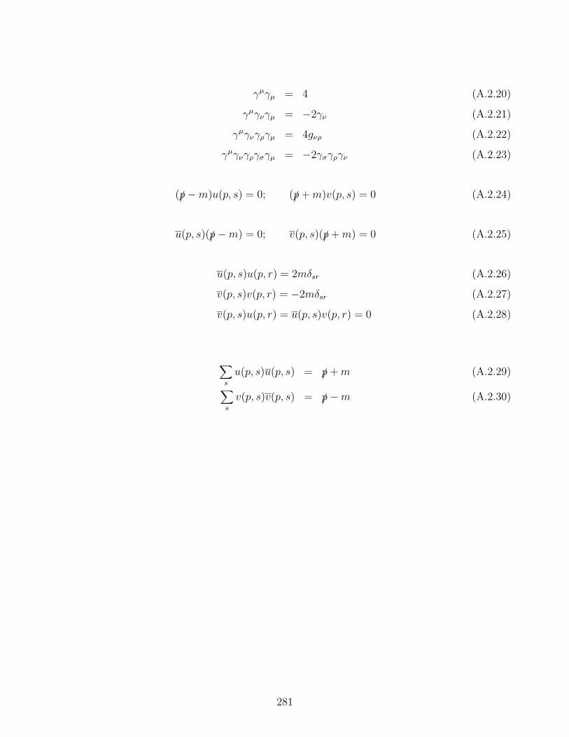
γµγµ = 4 (A.2.20)

γµγνγµ = −2γν (A.2.21)

γµγνγργµ = 4gνρ (A.2.22)

γµγνγργσγµ = −2γσγργν (A.2.23)

(/p−m)u(p, s) = 0; (/p+m)v(p, s) = 0 (A.2.24)

u(p, s)(/p−m) = 0; v(p, s)(/p+m) = 0 (A.2.25)

u(p, s)u(p, r) = 2mδsr (A.2.26)

v(p, s)v(p, r) = −2mδsr (A.2.27)

v(p, s)u(p, r) = u(p, s)v(p, r) = 0 (A.2.28)

∑

s

u(p, s)u(p, s) = /p+m (A.2.29)

∑

s

v(p, s)v(p, s) = /p−m (A.2.30)

281

Index

Abelian (commutative) group, 181

action, 25, 47, 49

active quarks, 211, 213

adjoint representation, 185, 186, 188, 189, 191,

193, 194, 198

Altarelli–Parisi (DGLAP) equations, 218, 223

angular momentum conservation, 115–117, 147,

155

angular momentum operator, 37

angular resolution, 122

annihilation operator, 54, 58, 59

anticommutation relations, 60, 61, 97

antineutrino, 150, 152

antineutrino-electron scattering, 167

antiparticle, 5, 7, 9, 41, 45–47, 59, 91, 111

associativity property of group, 180

asymptotic freedom, 212, 215

ATLAS detector at LHC, 233

BaBar experiment, 153

bare coupling, 207, 209

bare mass, 208, 209

barn (unit of cross-section), 68, 279

barred Dirac spinor, 35

baryons, 7–9

(J = 1/2), 8

(J = 3/2), 8, 9

Belle experiment, 153

beta function, 210, 211, 214, 215

QCD, 211

QED, 214

Bhabha scattering, 118

biunitary transformation, 259

boost, 16, 23, 33, 34

Bose-Einstein statistics, 56

bottomonium, 10–12, 233

branching ratios, 13, 146

charged pion, 152, 171

Higgs boson, 146, 258

lepton-number violating limits, 153

W boson, 263

Z boson, 250

Breit-Wigner lineshape, 5, 233

Cabibbo angle, 262, 263

Cabibbo-Kobayashi-Maskawa (CKM) mixing,

262, 263

canonical commutation relations, 37

canonical quantization

complex scalar field, 173

Dirac fermion fields, 61

real scalar fields, 53, 54

Carbon-14 dating, 150, 151

Casimir invariant, 184

charge conjugation, 162

charge conservation, 26, 27

charge density, 26

charge operator, 92

charged current, 168, 169, 178

charmonium, 10, 11, 233

chiral (Weyl) representation of Dirac matrices,

31, 280

chiral representations (of gauge group), 255

chiral symmetry breaking, 8, 244, 258, 259

closure property of group, 180, 182

CMS detector at LHC, 233

color, 5, 7

confinement, 5, 7, 107, 215

282

sum over, 201

commutation relations, 53–55

commutative (Abelian) group, 181

commutator of Lie algebra generators, 182

complex conjugate of spinor expressions, 101,

119, 155–157, 169

complex conjugate representation, 184

complex scalar field, 172

Compton scattering, 130–138

confinement of color, 5, 7, 107, 215

conservation of angular momentum, 115–117,

147, 155

conservation of charge, 26, 27

conservation of energy, 65, 78, 150

conservation of helicity, 117, 172

conservation of lepton number (or not), 153,

154, 265, 266

conservation of momentum, 18, 71, 98, 99

contravariant four-vector, 15, 16, 18, 24

Coulomb potential, 122

coupling

bare, 207, 209

electromagnetic (e), 53, 92, 248

electroweak (g), 178, 245, 246, 248

electroweak (g′), 246–248

Fermi (GF ), 156, 162

general, 88

QCD (g3, αs), 199–202, 211

experimental value, 213, 214

renormalized, 207–209, 248

scalar3, 77

scalar4, 62

scalarn, 85, 88

Yang-Mills gauge, 193–197, 239

Yukawa, 89, 143, 145, 146, 256–260

Yukawa, neutrino, 264

covariant derivative

QED, 94, 180

Yang-Mills, 193

covariant four-vector, 18

CPT Theorem, 162

creation operator, 54

fermionic, 58, 59

cross-section, 67–69

differential, 72

two particle → two particle, 76

crossing, 123–128, 138, 139, 165, 167

CTEQ parton distribution functions, 220

current density, electromagnetic, 26, 53, 92

cutoff, 57, 86, 99, 163, 176, 205–209, 213

decay rate (width, Γ), 140

defining representation, 182

density of states, 72

DGLAP equations, 218, 223

differential cross-section, 72

dimension of group (dG), 182, 184

dimension of representation (dR), 182

dimension of tensor product representation, 185

dimensional analysis, 161, 175, 176

dimensional regularization, 213

dimensional transmutation, 213

Dirac equation, 29–32

Dirac field, 47, 50, 51, 58–61

Dirac matrices, 31, 32, 280

Dirac spinor, 30, 31

direct sum representation, 184

double-counting problem, identical particles in

final state, 76, 128, 139, 143

Drell-Yan scattering, 231, 232

electroweak Standard Model (Glashow-Weinberg-

283

Salam) gauge theory, 245–249, 251–255

electroweak vector boson interactions, 253, 254

energy conservation, 65, 78, 150

ǫµνρσ (Levi-Civita) tensor, 25

equal-time commutators, 53

equivalence of representations of group, 183

ηb (scalar bottomonium), 10

ηc (scalar charmonium), 10

η meson, 233

Euler-Lagrange equations of motion, 47–51, 61

factorization scale, 218

femtobarns (fb), 68

Fermi constant (GF ), 156

numerical value, 161

relation to mW , 178

relation to Higgs VEV, 253

Fermi weak interaction theory, 156

Fermi-Dirac statistics, 59, 97

fermion-antifermion condensate, 244

Feynman diagram, 66, 82–84, 86, 87

Feynman gauge, 97, 98, 128, 195

Feynman propagator

charged massive vector fields, 177

Dirac fields, 90, 98

generic fields, 89

gluons, 199

Higgs boson, 241

massive vector fields, 179

photon, 96, 97

scalar, complex (π±), 173

scalar, real, 85

W boson, 177

Yang-Mills vector fields, 194

Feynman rules, 66

Fermi weak interaction theory, 156, 157

fermion external lines, 91

fermions with known helicity, 111

general, 87–90

massive vector bosons, 179

pion decay, 173–175

QCD, 199, 200

QED, 94–99

scalar φn theory, 84–86, 88

standard electroweak gauge theory, 253–255

W -fermion-antifermion, 178

Yang-Mills, 194–197

Yukawa coupling, 88, 89

Yukawa coupling, electron, 256

Feynman slash notation, 32

Feynman’s x, 217

Feynman-Stuckelberg interpretation, 40

field, 46, 47

Dirac, 47, 50, 51, 58–61

electromagnetic, 25, 26, 47, 52, 53

Majorana, 45, 50, 265

scalar, 46, 47, 49, 50

vector, 47, 50, 52, 53

Weyl, 50

field theory, 47

fine structure constant, 92, 104

flavors of quarks, 6, 7

four-fermion interaction, 156, 175, 177

four-vector, 15–17, 22

free field theory, 61

fundamental representation, 182

gµν (metric tensor), 17

γ (gamma) matrices, 31

traces, 280, 281

γ5 matrix, 39, 280

gauge eigenstate fields, 247, 260–262

284

gauge fixing, 96, 97

gauge-fixing parameter (ξ), 96, 97

gauge invariance, 27, 94, 180

Yang-Mills, 181, 191–196

Gell-Mann matrices, 189

generators

SU(2), 186

SU(3), 189

SU(N), 188

of Lie algebra, 182, 183

GeV, 29

global symmetry, 188, 235

global symmetry breaking, 236–238

glueballs, 12

gluon, 169, 198, 199

propagator, 199

gluon collider, 228

gluon-gluon scattering, 225–227

gluonium, 12

Goldstone boson, 238, 243

pseudo, 244

would-be, 241, 243, 251

Goldstone’s theorem, 243

Grassmann (anticommuting) numbers, 60

gravity, 177, 209

group, 23, 180

hadron-hadron scattering, 215–220, 228–232

hadronization, 216

hadrons, 7

half life, 150

Hamilton’s principle, 47

Hamiltonian

free Dirac field, 61

free scalar field, 54, 56, 57

general classical system, 53

interaction, 62, 63, 90

single Dirac particle, 30, 37

single scalar particle, 28

hard scattering of partons, 215

helicity, 38, 39

helicity conservation, 117, 172

helicity flip, 172

helicity suppression, 172

Higgs boson, 7, 8, 89, 145–147, 252–255, 270

discovery, 266

experimental mass, 7

interactions with Z,W, h, 253–255

mass in Standard Model, 255

Higgs field

generic, 239, 241, 243, 245

Standard Model, 250–255

Higgs mechanism, 239, 241, 243, 245

hole (absence of an electron), 40

identical final state particle overcounting prob-

lem, 76, 128, 139, 143

identity element of group, 180

iǫ factor in propagators, 85

ignorance, parameterization of, 169, 170, 207

IN state, 63, 64

index of representations, 183

SU(2), 187

SU(3), 189

adjoint, 185

inertial reference frame, 15

infinite momentum frame, 217

infrared slavery, 212

integrated luminosity, 67

interaction Hamiltonian, 62, 63, 90

interaction Lagrangian, 62

internal line, 82

285

inverse metric tensor (gµν), 17

inverse muon decay, 165

inverse of group element, 180

irreducible representation, 184

isospin global symmetry, 188

Jacobi identity, 183

Jacobian, 230, 232

jet, 107, 200, 216

J/ψ (vector charmonium), 11, 108, 233

Klein-Gordon equation, 29, 35, 50

Klein-Nishina formula for Compton scattering,

137

Lagrangian, 47, 49

Lagrangian density, 49

Landau gauge, 97, 98, 195

Large Hadron Collider (LHC), 4, 145, 222, 224,

226–228, 233, 271

lattice gauge theory, 13

left-handed fermions

and weak interactions, 155, 156, 168, 188,

245, 246, 255

Dirac, 39

projection matrix (PL), 39, 41

Weyl, 44, 45

left-handed polarization of photon, 95

lepton number (total), 154, 265, 266

lepton numbers (individual), 153, 154

leptons, 6

Levi-Civita (ǫµνρσ) tensor, 25

Lie algebra, 182, 183

Lie group, 181

linear collider, 110

local (gauge) symmetry, 180, 235

breaking, 239–241, 243

longitudinal momentum fraction (Feynman’s x),

217

longitudinal polarization of massive vector bo-

son, 241

longitudinal rapidity, 21, 229

loop corrections to muon decay, 163

loops in Feynman diagrams, 86, 90, 99, 176,

196, 204–206, 208, 209, 258

fermion minus sign, 99

Lorentz transformations, 15, 16, 23

Lorentz-invariant phase space

n-body, 74, 141

2-body, 74, 75, 135, 142

3-body, 148, 149

lowering operator, 54–56

luminosity, 67

Majorana fermion, 45, 265, 266

Majorana field, 265

Mandelstam variables (s, t, u), 84, 119

Mandelstam variables, partonic (s, t, u), 216,

223

mass diagonalization, 259

mass eigenstate fields, 247, 260–262

massive vector boson, 179, 197, 240–243, 245,

247

propagator, 179

matrix element, 66, 67, 71

reduced, 71

Maxwell’s equations, 25–27, 52

mean lifetime, 141

MEG, 153

mesons, 7, 9, 10

(J = 0), 9, 10

(J = 1), 10

metric tensor (gµν), 17

286

Mexican hat potential, 236

Møller scattering, 126

momentum conservation, 18, 71, 98, 99

momentum fraction (Feynman’s x), 217

MS renormalization scheme, 213, 248

MSTW parton distribution functions, 220

muon decay, 152, 156–161

muon production in e−e+ collisions, 100–105

Nambu-Goldstone boson, 238, 243

pseudo, 244

would-be, 241, 243, 251

nanobarns (nb), 68

natural units, 279

neutrino, 6, 44

anti-, 7, 150, 152

masses, 264–266

mixing, 265

seesaw mechanism, 264, 265

Yukawa coupling, 264

neutrinoless double beta decay, 266

neutron, 7

neutron decay, 150

non-Abelian gauge invariance, 181, 191–194

non-renormalizable theories, 176, 177, 197, 209

nuclear weak decays, 150, 151

nucleons, 7

ω meson, 233

on-shell, 18

OUT state, 63, 64

overcounting problem for identical final state

particles, 76, 128, 139, 143

parity, 23, 154, 162

parity violation, 23, 155, 156

partial width, 13, 141

Particle Data Group, 4

parton, 215, 217

parton distribution function (PDF), 217–223

parton model, 215

partonic subprocess, 215, 216

Pauli exclusion principle, 40, 59

Pauli matrices (σ1,2,3), 30, 280

φ meson, 233

photon field (Aµ), 47, 92, 94–97

photon polarization, 95, 96

photon propagator, 96–98

picobarns (pb), 68

pion (π±) decay, 169–175

pion decay constant (fπ), 170

polarization vector, 95

and gauge transformations, 129

massive vector boson, 179

polarized beams, 110

Pontecorvo-Maki-Nakagawa-Sakata (PMNS) ma-

trix, 265

positron, 30, 40

potential energy, 47, 48, 235

projection matrices for helicity (PL, PR), 39,

280

propagator

charged massive vector boson, 177, 179

Dirac fermion, 90, 98

generic, 89

gluon, 199

Higgs boson, 241

massive vector boson, 177, 179

photon, 96, 97

scalar, complex (π±), 173

scalar, real, 85

W boson, 177

287

Yang-Mills vector fields, 194

proper interval, 17

proper Lorentz transformations, 23

proton, 7

pseudo-Nambu-Goldstone boson, 244

pseudo-rapidity, 21

pseudo-scalar fermion bilinear, 154

QCD coupling, 199–202, 211

experimental value, 213, 214

QCD scale (ΛQCD), 211, 212

quadratic Casimir invariant, 184

Quantum Chromo-Dynamics (QCD), 107, 188,

198–200

Quantum Electro-Dynamics (QED), 92–94

Feynman rules, 94–99

quark, 6

flavors, 6, 7

masses, 6, 7, 258, 259

quark-antiquark condensate, 244

quark-quark scattering, 200–202

quarkonium, 11, 12

raising operator, 54–56

rapidity, 16, 34, 36

longitudinal, 21, 229

pseudo-, 21

reduced matrix element, 71

reducible representation, 183

regularization, 57, 86, 176, 205, 213

renormalizable theories, 176, 177

renormalization, 57, 86, 163, 164

renormalization group, 210

renormalization scale, 207–210, 218

renormalized (running) coupling, 207–209

electroweak, 248

renormalized (running) mass, 208, 209

representation of group, 181

representations

of SU(2), 186–188

of SU(3), 188–190

of SU(N), 191

of U(1), 181

of non-Abelian group, 181–186

Review of Particle Properties (Particle Data

Group), 4, 108

Rhadrons, 108, 110

ρ meson, 233

right-handed antifermions and weak interactions,

155, 166

right-handed fermions

Dirac, 39

Weyl, 44

right-handed polarization of photon, 95

right-handed projection matrix (PR), 41

rotations, 23

Rutherford scattering, 122

scalar field, 46, 47, 49, 50

complex, 172

scalar function, 24

s-channel, 82, 84

Schrodinger equation, 28

Schrodinger picture of quantum mechanics, 62,

63

sea partons, 217, 219, 221

sea quarks, 8, 219

seesaw mechanism for neutrino masses, 264, 265

singlet representation, 181, 184

slash notation, 32

speed of light (c), 15, 279

spin operator, 37

spin-sum identities, 42, 281

288

spinor, 30

Dirac, 31

Majorana, 45

Weyl, 44

spontaneous symmetry breaking, 235

global, 235–238

local (gauge), 239–241

Standard Model, 245–249, 251–255

structure constants of non-Abelian group, 182

SU(2) Lie algebra, 186–188

SU(2)L (weak isospin), 188, 245, 246

SU(3) Lie algebra, 188–190

SU(N) Lie algebra, 188, 191

subprocess, partonic, 215, 216

supersymmetry, 45, 222, 228

symmetry factor (of Feynman diagram), 86, 87,

99

tau decays, 13

t-channel, 83, 84, 118

technicolor, 244

tensor, 24

tensor product of representations, 185

Tevatron, 68, 69, 222, 224, 228

Thomson scattering, 137

three-body phase space, 147–149

time reversal (T), 22, 23, 162

top quark, 6, 7

decay, 263

LHC production cross-section, 69, 226–228

Tevatron production cross-section, 69, 224–

226, 228

trace trick, 102, 103

traces of γ matrices, 32, 102, 280, 281

transverse momentum (pT ), 229

transverse polarization, 95, 240

tree-level diagrams, 85

triangle function (λ), 142

two-body phase space, 135

U(1) as a Lie group, 181

U(1) for electromagnetism, 181, 198

U(1)Y (weak hypercharge), 245, 246, 249–251

u-channel, 83, 84

unitarity of CKM matrix, 263

unitarity of quantum mechanical time evolu-

tion, 175, 177, 197

unitary gauge, 241, 242

Standard Model, 251–254

units, 29, 279

Υ (vector bottomonium), 11, 233

vacuum expectation value (VEV), 236

antiquark-quark, 244

Standard Model, 251

Standard Model numerical, 252

vacuum state, 46, 55, 59

valence quarks, 8, 169, 217, 219, 221, 226

volume element, 25

W boson, 5

branching ratios, 263

couplings to fermions, 261, 262

interactions with Z,W, h, 253, 254

mass, measured, 5

mass, prediction, 252

width, measured, 5

width, predicted, 6

Ward identity, 129, 130

weak hypercharge [U(1)Y ], 245, 246, 249–251

weak isospin [SU(2)L], 188, 245, 246

weak mixing angle θW , 247

289

weak mixing angle (Weinberg angle) θW , 248,

249, 252, 253

weak-interaction charged current, 168, 169, 178

Weyl (chiral) representation of Dirac matrices,

31, 280

Weyl equation, 44

Weyl fermion, 44

Weyl spinor, 44

would-be Nambu-Goldstone boson, 241, 243,

251

Standard Model, 251

x, Feynman (momentum fraction), 217

ξ (gauge-fixing parameter), 96, 97

Yang-Mills theories, 179, 191–196

Yukawa coupling, 89, 143, 145, 146, 256–260

neutrino, 264

Z boson, 5, 232

branching ratios, 250

couplings to fermions, 249, 250

interactions with Z,W, h, 253, 254

mass, measured, 5

mass, prediction, 252

resonance at LHC, 233

width, 5

290