Phenotypic variability of growing cellular populationsTing Lu*†, Tongye Shen†‡, Matthew R. Bennett§¶, Peter G. Wolynes*†‡, and Jeff Hasty§¶�

Departments of *Physics, ‡Chemistry and Biochemistry, and §Bioengineering, †Center for Theoretical Biological Physics, and ¶Institute for Nonlinear Science,University of California at San Diego, La Jolla, CA 92093

Edited by Charles R. Cantor, Sequenom Inc., San Diego, CA, and approved October 2, 2007 (received for review June 29, 2007)

The dynamics and diversity of proliferating cellular populations aregoverned by the interplay between the growth and death ratesamong the various phenotypes within a colony. In addition, epige-netic multistability can cause cells to spontaneously switch from onephenotype to another. By examining a generalized form of therelative variance of populations and classifying it into intracolony andcross-colony contributions, we study the origins and consequences ofcellular population variability. We find that the variability can dependhighly on the initial conditions and the constraints placed on thepopulation by the growth environment. We construct a two-pheno-type model system and examine, analytically and numerically, itstime-dependent variability in both unbounded and population-lim-ited growth environments. We find that in unbounded growthenvironments the overall variability is strictly governed by the initialconditions. In contrast, when the overall population is limited by theenvironment, the system eventually relaxes to a unique fixed pointregardless of the initial conditions. However, the transient decay tothe fixed point depends highly on initial conditions, and the time scaleover which the variability decays can be very long, depending on theintrinsic time scales of the system. These results provide insights intothe origins of population variability and suggest mechanisms in whichvariability can arise in commonly used experimental approaches.

cellular population diversity � gene noise � phenotyic variation

Cellular populations are rarely collections of homogeneous celltypes, even when the cells share the same genetic makeup.

Differences in cell size, growth rate, and morphology are commonand greatly contribute to the overall variability of the population.Often, these variations are due to stochastic fluctuations that canoccur at many different scales (1–4). For instance, noise contributesto the traversal of start and progression of yeast cells into the cellcycle (5) and can limit the precision of circadian clocks (6).Furthermore, noise plays an important role in determining thephenotype of cells that exhibit epigenetic multistability. In suchcases, the same set of genes can lead to drastically differentphenotypic expression depending on the current state of the genes.Epigenetic multistability has been found to play a role in many genenetworks including metabolic systems (7–9) and bacterial persis-tence (10–12). Similarly, noise also appears to underlie the emer-gence of neural precursor cells from an initially homogeneouspopulation during the development of Drosophila melanogaster(13), and random fluctuations influence the fates of cells infectedwith HIV (14).

Noise occurring at both the genetic and molecular level has beenintensively studied in the past few years (1–3, 15–18), and multiplesources can contribute to the observed variability (19). Researchershave classified noise into two general classes: intrinsic noise, whichstems from the low numbers of reactants involved in gene expres-sion and regulation, and extrinsic noise, which arises from all othersources such as environmental fluctuations (20, 21). Noise in geneexpression can be propagated through network cascades, and thecorresponding amplitude of the fluctuation (as measured by aprotein concentration, for instance) is affected by the details of thenetwork (22–26). However, variability at the molecular level is oftennot the sole consequence of stochastic fluctuations. Genetic noisecan lead to macroscopic level fluctuations of entire cellular popu-lations because different types of cells usually have distinct re-sponses to various environments and will therefore have different

growth rates and survival capabilities (20, 21, 27–29). Additionally,the switching of individual cells from one epigenetic phenotype toanother can lead to dramatic changes in the overall variability of anentire population (30). Diversity of cellular populations, as mea-sured by the overall numbers of specific phenotypes (31–33), istherefore expected to be affected by the stochasticity inherent togene regulation.

In this article, we study the effects of epigenetic multistability onpopulation diversity. We first introduce a generalized form of therelative variance (the square of the coefficient of variation), whichis closely related to Simpson’s index (34) and takes into account thevariability both within a single colony and between multiple, distinctpopulations. Next, using a two-phenotype community as an exam-ple, we analytically and numerically investigate the propagation ofthe relative variance in different environments. We find that thevariation in a population depends highly on its initial state andcorresponding environments: Different initial conditions result inpermanent differences of variation in unbounded growth environ-ments, whereas variability arising from initial conditions in growth-limited environments (such as logistic growth or microfluidicchemostats) eventually decays away. However, this transient decayof the variability can occur on time scales that are longer than thetypical duration of many experimental procedures. Furthermore,the type of growth limitation placed on the population can affect thefinal steady-state variability. Therefore, our findings suggest thatcare must be taken when designing experiments to measure thevariability of multistable cellular populations. If the transients arenot given a sufficient amount of time to decay or the type of growthlimitation is not taken into account, then conclusions drawn fromsuch experiments may be faulty.

ResultsGeneralized Relative Variance. To illustrate the effects of stochas-ticity on cellular population variability, we examined the simpletwo-phenotype community shown in Fig. 1a. Each type of cell candivide, die, and switch to the other type. We assume that the cellsgrow in an idealized microfluidic chemostat-like environment (35)in which there is a maximum possible number of cells (Nmax, say)but that the growth rates of the cells are not limited by the overallpopulation. In such an environment, once the population maximumis reached, subsequent cellular divisions are still possible, but thispopulation growth begins to push cells out of the chemostat. Tosimulate this, we used a modified version of Gillespie’s algorithm(36). Each time the total population reached Nmax � 1, one cell(chosen at random) was taken out of the population. The simula-tions were run for a finite amount of time, representing six doublingtimes of the fastest growing phenotype, which is typical for exper-

Author contributions: T.L., T.S., M.R.B., P.G.W., and J.H. designed research; T.L. and T.S.performed research; T.L., T.S., and M.R.B. analyzed data; and T.L., T.S., M.R.B., P.G.W., andJ.H. wrote the paper.

The authors declare no conflict of interest.

This article is a PNAS Direct Submission.

�To whom correspondence should be addressed at: 9500 Gilman Drive MC0412, La Jolla,CA 92093. E-mail: hasty@bioeng.ucsd.edu.

This article contains supporting information online at www.pnas.org/cgi/content/full/0706115104/DC1.

© 2007 by The National Academy of Sciences of the USA

18982–18987 � PNAS � November 27, 2007 � vol. 104 � no. 48 www.pnas.org�cgi�doi�10.1073�pnas.0706115104

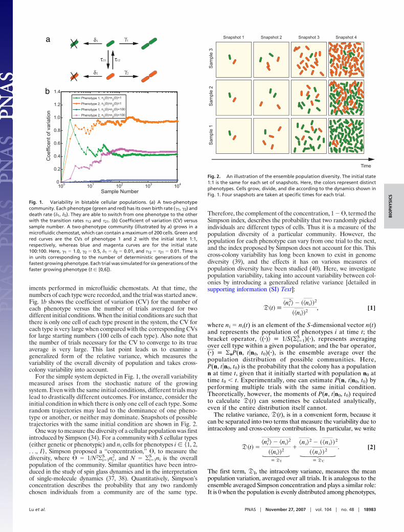
iments performed in microfluidic chemostats. At that time, thenumbers of each type were recorded, and the trial was started anew.Fig. 1b shows the coefficient of variation (CV) for the number ofeach phenotype versus the number of trials averaged for twodifferent initial conditions. When the initial conditions are such thatthere is only one cell of each type present in the system, the CV foreach type is very large when compared with the corresponding CVsfor large starting numbers (100 cells of each type). Also note thatthe number of trials necessary for the CV to converge to its trueaverage is very large. This last point leads us to examine ageneralized form of the relative variance, which measures thevariability of the overall diversity of population and takes cross-colony variability into account.

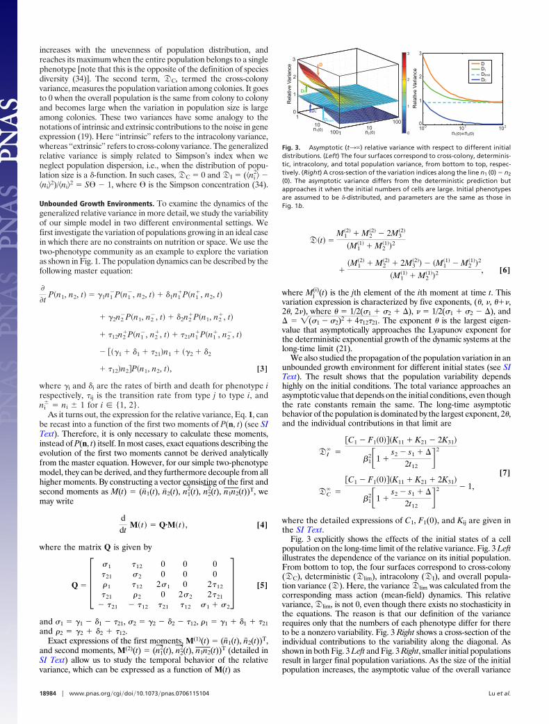
For the simple system depicted in Fig. 1, the overall variabilitymeasured arises from the stochastic nature of the growingsystem. Even with the same initial conditions, different trials maylead to drastically different outcomes. For instance, consider theinitial condition in which there is only one cell of each type. Somerandom trajectories may lead to the dominance of one pheno-type or another, or neither may dominate. Snapshots of possibletrajectories with the same initial condition are shown in Fig. 2.

One way to measure the diversity of a cellular population was firstintroduced by Simpson (34). For a community with S cellular types(either genetic or phenotypic) and ni cells for phenotypes i � {1, 2,. . ., I}, Simpson proposed a ‘‘concentration,’’ �, to measure thediversity, where � � 1/N2�i�1

S ni2, and N � �i�1

S ni is the overallpopulation of the community. Similar quantities have been intro-duced in the study of spin glass dynamics and in the interpretationof single-molecule dynamics (37, 38). Quantitatively, Simpson’sconcentration describes the probability that any two randomlychosen individuals from a community are of the same type.

Therefore, the complement of the concentration, 1 � �, termed theSimpson index, describes the probability that two randomly pickedindividuals are different types of cells. Thus it is a measure of thepopulation diversity of a particular community. However, thepopulation for each phenotype can vary from one trial to the next,and the index proposed by Simpson does not account for this. Thiscross-colony variability has long been known to exist in genomediversity (39), and the effects it has on various measures ofpopulation diversity have been studied (40). Here, we investigatepopulation variability, taking into account variability between col-onies by introducing a generalized relative variance [detailed insupporting information (SI) Text]:

��t� ��ni

2 � ��ni�2

��ni�2 , [1]

where ni � ni(t) is an element of the S-dimensional vector n(t)and represents the population of phenotypes i at time t; thebracket operator, �(�) 1/S(�i�1

S )(�), represents averagingover cell type within a given population; and the bar operator,(�) �nP(n, t�n0, t0)(�), is the ensemble average over thepopulation distribution of possible communities. Here,P(n, t�n0, t0) is the probability that the colony has a populationn at time t, given that it initially started with population n0 attime t0 � t. Experimentally, one can estimate P(n, t�n0, t0) byperforming multiple trials with the same initial condition.Theoretically, however, the moments of P(n, t�n0, t0) requiredto calculate �(t) can sometimes be calculated analytically,even if the entire distribution itself cannot.

The relative variance, �(t), is in a convenient form, because itcan be separated into two terms that measure the variability due tointracolony and cross-colony contributions. In particular, we write

��t� ��ni

2 � �ni2

��ni�2

Ç �I

��ni

2 � ��ni�2

��ni�2

Ç �C

. [2]

The first term, �I, the intracolony variance, measures the meanpopulation variation, averaged over all trials. It is analogous to theensemble averaged Simpson concentration and plays a similar role:It is 0 when the population is evenly distributed among phenotypes,

Phenotype 1, n1(0)=n

2(0)=1

Phenotype 2, n1(0)=n

2(0)=1

Phenotype 1, n1(0)=n

2(0)=100

Phenotype 2, n1(0)=n

2(0)=100

100 101 102 103 1040

0.2

0.4

0.6

0.8

1.0

1.2

1.4

Sample Number

Coe

ffice

nt o

f var

iatio

n

γ1δ1

γ2δ2

τ12τ21

a

b

Fig. 1. Variability in bistable cellular populations. (a) A two-phenotypecommunity. Each phenotype (green and red) has its own birth rate (�1, �2) anddeath rate (�1, �2). They are able to switch from one phenotype to the otherwith the transition rates �12 and �21. (b) Coefficient of variation (CV) versussample number. A two-phenotype community (illustrated by a) grows in amicrofluidic chemostat, which can contain a maximum of 200 cells. Green andred curves are the CVs of phenotype 1 and 2 with the initial state 1:1,respectively, whereas blue and magenta curves are for the initial state100:100. Here, �1 � 1.0, �2 � 0.5, �1 � �2 � 0.01, and �12 � �21 � 0.01. Time isin units corresponding to the number of deterministic generations of thefastest growing phenotype. Each trial was simulated for six generations of thefaster growing phenotype (t � [0,6]).

Time

Snapshot 1 Snapshot 2 Snapshot 3 Snapshot 4

Sam

ple

3S

ampl

e 1

Sam

ple

2

Fig. 2. An illustration of the ensemble population diversity. The initial state1:1 is the same for each set of snapshots. Here, the colors represent distinctphenotypes. Cells grow, divide, and die according to the dynamics shown inFig. 1. Four snapshots are taken at specific times for each trial.

Lu et al. PNAS � November 27, 2007 � vol. 104 � no. 48 � 18983

BIO

PHYS

ICS

increases with the unevenness of population distribution, andreaches its maximum when the entire population belongs to a singlephenotype [note that this is the opposite of the definition of speciesdiversity (34)]. The second term, �C, termed the cross-colonyvariance, measures the population variation among colonies. It goesto 0 when the overall population is the same from colony to colonyand becomes large when the variation in population size is largeamong colonies. These two variances have some analogy to thenotations of intrinsic and extrinsic contributions to the noise in geneexpression (19). Here ‘‘intrinsic’’ refers to the intracolony variance,whereas ‘‘extrinsic’’ refers to cross-colony variance. The generalizedrelative variance is simply related to Simpson’s index when weneglect population dispersion, i.e., when the distribution of popu-lation size is a �-function. In such cases, �C � 0 and �I � (�ni

2 ��ni2)/�ni2 � S� � 1, where � is the Simpson concentration (34).

Unbounded Growth Environments. To examine the dynamics of thegeneralized relative variance in more detail, we study the variabilityof our simple model in two different environmental settings. Wefirst investigate the variation of populations growing in an ideal casein which there are no constraints on nutrition or space. We use thetwo-phenotype community as an example to explore the variationas shown in Fig. 1. The population dynamics can be described by thefollowing master equation:

�

�tP�n1, n2, t� � �1n1

�P�n1�, n2, t� � �1n1

�P�n1�, n2, t�

� �2n2�P�n1, n2

�, t� � �2n2�P�n1, n2

�, t�

� �12n2�P�n1

�, n2�, t� � �21n1

�P�n1�, n2

�, t�

� ���1 � �1 � �21�n1 � ��2 � �2

� �12�n2 P�n1, n2, t�, [3]

where �i and �i are the rates of birth and death for phenotype irespectively, �ij is the transition rate from type j to type i, andni

� � ni � 1 for i � {1, 2}.As it turns out, the expression for the relative variance, Eq. 1, can

be recast into a function of the first two moments of P(n, t) (see SIText). Therefore, it is only necessary to calculate these moments,instead of P(n, t) itself. In most cases, exact equations describing theevolution of the first two moments cannot be derived analyticallyfrom the master equation. However, for our simple two-phenotypemodel, they can be derived, and they furthermore decouple from allhigher moments. By constructing a vector consisting of the first andsecond moments as M(t) � (n�1(t), n�2(t), n1

2(t), n22(t), n1n2(t))T, we

may write

ddt

M� t� � Q�M� t� , [4]

where the matrix Q is given by

Q � ��1 �12 0 0 0�21 �2 0 0 01 �12 2�1 0 2�12

�21 2 0 2�2 2�21

� �21 � �12 �21 �12 �1 � �2

� [5]

and �1 � �1 � �1 � �21, �2 � �2 � �2 � �12, 1 � �1 � �1 � �21

and 2 � �2 � �2 � �12.Exact expressions of the first moments, M(1)(t) � (n�1(t), n�2(t))T,

and second moments, M(2)(t) � (n12(t), n2

2(t), n1n2(t))T (detailed inSI Text) allow us to study the temporal behavior of the relativevariance, which can be expressed as a function of M(t) as

��t� �M1

�2� � M2�2� � 2M3

�2�

�M1�1� � M2

�1��2

��M1

�2� � M2�2� � 2M3

�2�� � �M1�1� � M2

�1��2

�M1�1� � M2

�1��2 , [6]

where Mj(i)(t) is the jth element of the ith moment at time t. This

variation expression is characterized by five exponents, (, �, ��,2, 2�), where � 1/2(�1 � �2 � �), � � 1/2(�1 � �2 � �), and� � �(�1 � �2)2 � 4�12�21. The exponent is the largest eigen-value that asymptotically approaches the Lyapunov exponent forthe deterministic exponential growth of the dynamic systems at thelong-time limit (21).

We also studied the propagation of the population variation in anunbounded growth environment for different initial states (see SIText). The result shows that the population variability dependshighly on the initial conditions. The total variance approaches anasymptotic value that depends on the initial conditions, even thoughthe rate constants remain the same. The long-time asymptoticbehavior of the population is dominated by the largest exponent, 2,and the individual contributions in that limit are

�I� �

�C1 � F1�0� �K11 � K21 � 2K31�

�12�1 �

s2 � s1 � �

2t12�2

�C� �

�C1 � F1�0� �K11 � K21 � 2K31�

�12�1 �

s2 � s1 � �

2t12�2 � 1,

[7]

where the detailed expressions of C1, F1(0), and Kij are given inthe SI Text.

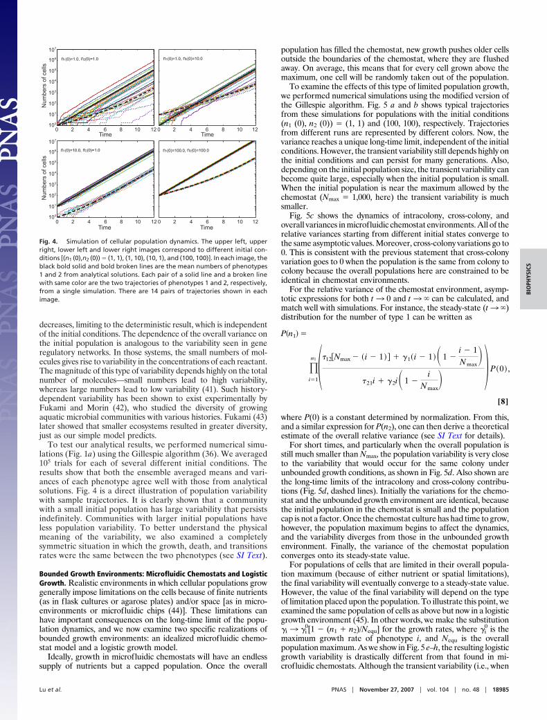
Fig. 3 explicitly shows the effects of the initial states of a cellpopulation on the long-time limit of the relative variance. Fig. 3 Leftillustrates the dependence of the variance on its initial population.From bottom to top, the four surfaces correspond to cross-colony(�C), deterministic (�lim), intracolony (�I), and overall popula-tion variance (�). Here, the variance �lim was calculated from thecorresponding mass action (mean-field) dynamics. This relativevariance, �lim, is not 0, even though there exists no stochasticity inthe equations. The reason is that our definition of the variancerequires only that the numbers of each phenotype differ for thereto be a nonzero variability. Fig. 3 Right shows a cross-section of theindividual contributions to the variability along the diagonal. Asshown in both Fig. 3 Left and Fig. 3 Right, smaller initial populationsresult in larger final population variations. As the size of the initialpopulation increases, the asymptotic value of the overall variance

1

10

100 1 10

100

0

1

2

3

n 1 n 2 (0)

(0)

Rel

ativ

e V

aria

nce

0

1

2

3

D C

D limit

D

D I

10 0 10 1 10 2 0

1

2

3

n 2 (0) n 1 (0) =

Rel

ativ

e V

aria

nce

D D I D limit

D C

Fig. 3. Asymptotic (t3�) relative variance with respect to different initialdistributions. (Left) The four surfaces correspond to cross-colony, determinis-tic, intracolony, and total population variance, from bottom to top, respec-tively. (Right) A cross-section of the variation indices along the line n1 (0) � n2

(0). The asymptotic variance differs from the deterministic prediction butapproaches it when the initial numbers of cells are large. Initial phenotypesare assumed to be �-distributed, and parameters are the same as those inFig. 1b.

18984 � www.pnas.org�cgi�doi�10.1073�pnas.0706115104 Lu et al.

decreases, limiting to the deterministic result, which is independentof the initial conditions. The dependence of the overall variance onthe initial population is analogous to the variability seen in generegulatory networks. In those systems, the small numbers of mol-ecules gives rise to variability in the concentrations of each reactant.The magnitude of this type of variability depends highly on the totalnumber of molecules—small numbers lead to high variability,whereas large numbers lead to low variability (41). Such history-dependent variability has been shown to exist experimentally byFukami and Morin (42), who studied the diversity of growingaquatic microbial communities with various histories. Fukami (43)later showed that smaller ecosystems resulted in greater diversity,just as our simple model predicts.

To test our analytical results, we performed numerical simu-lations (Fig. 1a) using the Gillespie algorithm (36). We averaged105 trials for each of several different initial conditions. Theresults show that both the ensemble averaged means and vari-ances of each phenotype agree well with those from analyticalsolutions. Fig. 4 is a direct illustration of population variabilitywith sample trajectories. It is clearly shown that a communitywith a small initial population has large variability that persistsindefinitely. Communities with larger initial populations haveless population variability. To better understand the physicalmeaning of the variability, we also examined a completelysymmetric situation in which the growth, death, and transitionsrates were the same between the two phenotypes (see SI Text).

Bounded Growth Environments: Microfluidic Chemostats and LogisticGrowth. Realistic environments in which cellular populations growgenerally impose limitations on the cells because of finite nutrients(as in flask cultures or agarose plates) and/or space [as in micro-environments or microfluidic chips (44)]. These limitations canhave important consequences on the long-time limit of the popu-lation dynamics, and we now examine two specific realizations ofbounded growth environments: an idealized microfluidic chemo-stat model and a logistic growth model.

Ideally, growth in microfluidic chemostats will have an endlesssupply of nutrients but a capped population. Once the overall

population has filled the chemostat, new growth pushes older cellsoutside the boundaries of the chemostat, where they are flushedaway. On average, this means that for every cell grown above themaximum, one cell will be randomly taken out of the population.

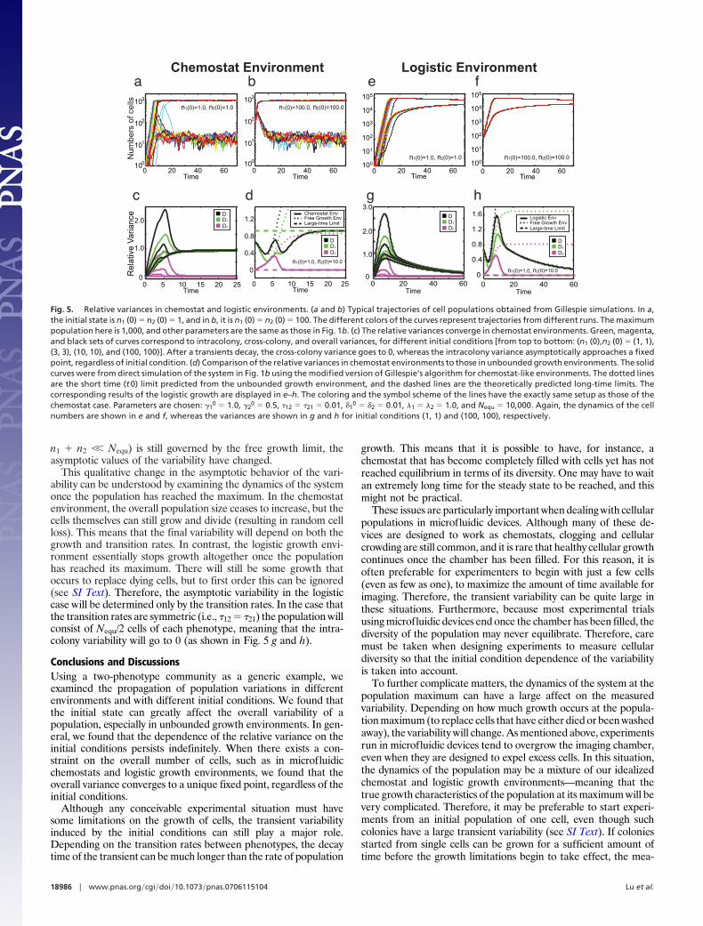
To examine the effects of this type of limited population growth,we performed numerical simulations using the modified version ofthe Gillespie algorithm. Fig. 5 a and b shows typical trajectoriesfrom these simulations for populations with the initial conditions(n1 (0), n2 (0)) � (1, 1) and (100, 100), respectively. Trajectoriesfrom different runs are represented by different colors. Now, thevariance reaches a unique long-time limit, independent of the initialconditions. However, the transient variability still depends highly onthe initial conditions and can persist for many generations. Also,depending on the initial population size, the transient variability canbecome quite large, especially when the initial population is small.When the initial population is near the maximum allowed by thechemostat (Nmax � 1,000, here) the transient variability is muchsmaller.

Fig. 5c shows the dynamics of intracolony, cross-colony, andoverall variances in microfluidic chemostat environments. All of therelative variances starting from different initial states converge tothe same asymptotic values. Moreover, cross-colony variations go to0. This is consistent with the previous statement that cross-colonyvariation goes to 0 when the population is the same from colony tocolony because the overall populations here are constrained to beidentical in chemostat environments.

For the relative variance of the chemostat environment, asymp-totic expressions for both t3 0 and t3 � can be calculated, andmatch well with simulations. For instance, the steady-state (t3 �)distribution for the number of type 1 can be written as

P�n1� �

i�1

n1 �12�Nmax � � i � 1� � �1� i � 1�� 1 �i � 1Nmax

��21i � �2i� 1 �

iNmax

� P�0� ,

[8]

where P(0) is a constant determined by normalization. From this,and a similar expression for P(n2), one can then derive a theoreticalestimate of the overall relative variance (see SI Text for details).

For short times, and particularly when the overall population isstill much smaller than Nmax, the population variability is very closeto the variability that would occur for the same colony underunbounded growth conditions, as shown in Fig. 5d. Also shown arethe long-time limits of the intracolony and cross-colony contribu-tions (Fig. 5d, dashed lines). Initially the variations for the chemo-stat and the unbounded growth environment are identical, becausethe initial population in the chemostat is small and the populationcap is not a factor. Once the chemostat culture has had time to grow,however, the population maximum begins to affect the dynamics,and the variability diverges from those in the unbounded growthenvironment. Finally, the variance of the chemostat populationconverges onto its steady-state value.

For populations of cells that are limited in their overall popula-tion maximum (because of either nutrient or spatial limitations),the final variability will eventually converge to a steady-state value.However, the value of the final variability will depend on the typeof limitation placed upon the population. To illustrate this point, weexamined the same population of cells as above but now in a logisticgrowth environment (45). In other words, we make the substitution�i 3 �i

0[1 � (n1 � n2)/Nequ] for the growth rates, where �i0 is the

maximum growth rate of phenotype i, and Nequ is the overallpopulation maximum. As we show in Fig. 5 e–h, the resulting logisticgrowth variability is drastically different from that found in mi-crofluidic chemostats. Although the transient variability (i.e., when

0 2 4 6 8 10 120 2 4 6 8 10 12100

101

102

103

104

105

106

107

0 2 4 6 8 10 120 2 4 6 8 10 12100

101

102

103

104

105

106

107

Time Time

Time Time

Num

bers

of c

ells

Num

bers

of c

ells

n2(0)=1.0n1(0)=1.0, n2(0)=10.0n1(0)=1.0,

n2(0)=1.0n1(0)=10.0, n2(0)=100.0n1(0)=100.0,

Fig. 4. Simulation of cellular population dynamics. The upper left, upperright, lower left and lower right images correspond to different initial con-ditions [(n1 (0),n2 (0)) � (1, 1), (1, 10), (10, 1), and (100, 100)]. In each image, theblack bold solid and bold broken lines are the mean numbers of phenotypes1 and 2 from analytical solutions. Each pair of a solid line and a broken linewith same color are the two trajectories of phenotypes 1 and 2, respectively,from a single simulation. There are 14 pairs of trajectories shown in eachimage.

Lu et al. PNAS � November 27, 2007 � vol. 104 � no. 48 � 18985

BIO

PHYS

ICS

n1 � n2 �� Nequ) is still governed by the free growth limit, theasymptotic values of the variability have changed.

This qualitative change in the asymptotic behavior of the vari-ability can be understood by examining the dynamics of the systemonce the population has reached the maximum. In the chemostatenvironment, the overall population size ceases to increase, but thecells themselves can still grow and divide (resulting in random cellloss). This means that the final variability will depend on both thegrowth and transition rates. In contrast, the logistic growth envi-ronment essentially stops growth altogether once the populationhas reached its maximum. There will still be some growth thatoccurs to replace dying cells, but to first order this can be ignored(see SI Text). Therefore, the asymptotic variability in the logisticcase will be determined only by the transition rates. In the case thatthe transition rates are symmetric (i.e., �12 � �21) the population willconsist of Nequ/2 cells of each phenotype, meaning that the intra-colony variability will go to 0 (as shown in Fig. 5 g and h).

Conclusions and DiscussionsUsing a two-phenotype community as a generic example, weexamined the propagation of population variations in differentenvironments and with different initial conditions. We found thatthe initial state can greatly affect the overall variability of apopulation, especially in unbounded growth environments. In gen-eral, we found that the dependence of the relative variance on theinitial conditions persists indefinitely. When there exists a con-straint on the overall number of cells, such as in microfluidicchemostats and logistic growth environments, we found that theoverall variance converges to a unique fixed point, regardless of theinitial conditions.

Although any conceivable experimental situation must havesome limitations on the growth of cells, the transient variabilityinduced by the initial conditions can still play a major role.Depending on the transition rates between phenotypes, the decaytime of the transient can be much longer than the rate of population

growth. This means that it is possible to have, for instance, achemostat that has become completely filled with cells yet has notreached equilibrium in terms of its diversity. One may have to waitan extremely long time for the steady state to be reached, and thismight not be practical.

These issues are particularly important when dealing with cellularpopulations in microfluidic devices. Although many of these de-vices are designed to work as chemostats, clogging and cellularcrowding are still common, and it is rare that healthy cellular growthcontinues once the chamber has been filled. For this reason, it isoften preferable for experimenters to begin with just a few cells(even as few as one), to maximize the amount of time available forimaging. Therefore, the transient variability can be quite large inthese situations. Furthermore, because most experimental trialsusing microfluidic devices end once the chamber has been filled, thediversity of the population may never equilibrate. Therefore, caremust be taken when designing experiments to measure cellulardiversity so that the initial condition dependence of the variabilityis taken into account.

To further complicate matters, the dynamics of the system at thepopulation maximum can have a large affect on the measuredvariability. Depending on how much growth occurs at the popula-tion maximum (to replace cells that have either died or been washedaway), the variability will change. As mentioned above, experimentsrun in microfluidic devices tend to overgrow the imaging chamber,even when they are designed to expel excess cells. In this situation,the dynamics of the population may be a mixture of our idealizedchemostat and logistic growth environments—meaning that thetrue growth characteristics of the population at its maximum will bevery complicated. Therefore, it may be preferable to start experi-ments from an initial population of one cell, even though suchcolonies have a large transient variability (see SI Text). If coloniesstarted from single cells can be grown for a sufficient amount oftime before the growth limitations begin to take effect, the mea-

Num

bers

of c

ells

Rel

ativ

e V

aria

nce

0 20 40 60Time

100

101

102

103

n2(0)=1.0n1(0)=1.0,

0 20 40 60Time

100

101

102

103

n2(0)=100.0n1(0)=100.0,

0 5 10 15 20 25Time

2.0

1.0

0

DDI

DC

0 5 10 15 20 25Time

0.4

0.8

1.2

0n2(0)=10.0n1(0)=1.0,

Chemostat EnvFree Growth EnvLarge-time Limit

100

101

102

103

104

105

0100

101

102

103

104

105

Time

Time

n2(0)=1.0n1(0)=1.0, n2(0)=100.0n1(0)=100.0,

e fa b

g hc d

0 20 40 600

0.4

0.8

1.2

1.6Logistic EnvFree Growth EnvLarge-time Limit

n2(0)=10.0n1(0)=1.0,

DDI

DC

Time0 20 40 60

0

1.0

2.0

3.0DDI

DC

20 40 600Time

20 40 60

DDI

DC

Chemostat Environment Logistic Environment

Fig. 5. Relative variances in chemostat and logistic environments. (a and b) Typical trajectories of cell populations obtained from Gillespie simulations. In a,the initial state is n1 (0) � n2 (0) � 1, and in b, it is n1 (0) � n2 (0) � 100. The different colors of the curves represent trajectories from different runs. The maximumpopulation here is 1,000, and other parameters are the same as those in Fig. 1b. (c) The relative variances converge in chemostat environments. Green, magenta,and black sets of curves correspond to intracolony, cross-colony, and overall variances, for different initial conditions [from top to bottom: (n1 (0),n2 (0) � (1, 1),(3, 3), (10, 10), and (100, 100)]. After a transients decay, the cross-colony variance goes to 0, whereas the intracolony variance asymptotically approaches a fixedpoint, regardless of initial condition. (d) Comparison of the relative variances in chemostat environments to those in unbounded growth environments. The solidcurves were from direct simulation of the system in Fig. 1b using the modified version of Gillespie’s algorithm for chemostat-like environments. The dotted linesare the short time (t 0) limit predicted from the unbounded growth environment, and the dashed lines are the theoretically predicted long-time limits. Thecorresponding results of the logistic growth are displayed in e–h. The coloring and the symbol scheme of the lines have the exactly same setup as those of thechemostat case. Parameters are chosen: �1

0 � 1.0, �20 � 0.5, �12 � �21 � 0.01, �1

0 � �2 � 0.01, 1 � 2 � 1.0, and Nequ � 10,000. Again, the dynamics of the cellnumbers are shown in e and f, whereas the variances are shown in g and h for initial conditions (1, 1) and (100, 100), respectively.

18986 � www.pnas.org�cgi�doi�10.1073�pnas.0706115104 Lu et al.

sured variability will be independent of the type of growthlimitation.

Materials and MethodsThe stochastic simulations in this study were performed with theGillespie algorithm (36) and consisted of the six events shown in Eq.2, where G and R represent the two different phenotypes (green andred in Fig. 1).

GO¡�1

2G GO¡�1

A

RO¡�2

2R RO¡�2

A [9]

GO¡�21

R RO¡�12

G.

For simulations involving unbounded growth environments, thepopulations were allowed to change freely. Simulations of popula-

tions in idealized chemostat environments were subjected to amaximum population constraint, limiting the total number of cellsto Nmax. These simulations were run in the same manner as theunbounded-growth environment simulations, except that each timethe total number of cells reached Nmax � 1, a single cell wasremoved from the population. The type of cell removed was chosenrandomly, with the probability of a cell of type i being removedgiven by ni/¥ini, where ni is the number of cells of type i. Simulationsof populations in logistic environments were performed in the samemanner as the unbounded growth environments except that growthrates depended on present populations, i.e., growth rates can beexpressed by �i � �i

0 (1 � ¥i ini/Nequ), where �i0 and i are the

corresponding rate and relative weight, and Nequ is the overallequilibrium population. Growth rates therefore are updated in thesimulation once the populations change. Simulations for each initialcondition were performed 105 times, and the populations of eachtype were recorded after each trial. The various measures ofvariability (CV and relative variance) were calculated according totheir definitions.

We thank Lev Tsimring and Dmitri Volfson for stimulating discussions.This work is supported by National Institutes of Health GrantsGM69811-01 and GM082168-01.

1. Rao CV, Wolf DM, Arkin AP (2002) Nature 420:231–237.2. Kaern M, Elston TC, Blake WJ, Collins JJ (2005) Nat Rev Genet 6:451–464.3. Smits WK, Kuipers OP, Veening JW (2006) Nat Rev Microbiol 4:259–271.4. Douglass JK, Wilkens L, Pantazelou E, Moss F (1993) Nature 365:337–340.5. Bean JM, Siggia ED, Cross FR (2006) Mol Cell 21:3–14.6. Barkai N, Leibler S (1999) Nature 403:267–268.7. Siegele DA, Hu JC (1997) Proc Natl Acad Sci USA 94:8168–8172.8. Biggar SR, Crabtree GR (2001) EMBO J 20:3167–3176.9. Thattai M, Shraiman B (2003) Biophys J 85:744–754.

10. Bigger JW (1944) Lancet 244:497–500.11. Kussell E, Kishnoy R, Balaban NQ, Leibler S (2005) Genetics 169:1807–1814.12. Levin BR, Rozen DE (2006) Nat Rev Microbiol 4:556–562.13. Simpson P (1997) Curr Opin Genet Dev 7:537–542.14. Weinberger L, Burnett JC, Toettcher JE, Arkin AP, Schaffer DV (2005) Cell

122:169–182.15. Graumann PL (2006) Mol Microbiol 61(3):560–563.16. Raser JM, O’Shea EK (2005) Science 309:2010–2013.17. Simpson ML, Cox CD, Sayler GS (2003) Proc Natl Acad Sci USA 100:4551–4556.18. Austin DW, Allen MS, McCollum JM, Dar RD, Wilgus JR, Sayler GS,

Samatova NF, Cox CD, Simpson ML (2006) Nature 439:608–611.19. Swain PS, Elowitz MB, Siggia ED (2002) Proc Natl Acad Sci USA 99:12795–12800.20. Thattai M, van Oudennarden A (2004) Genetics 167:523–530.21. Kussell E, Leibler S (2005) Science 309:2075–2078.22. Shen-Orr SS, Milo R, Mangan S, Alon U (2002) Nat Genet 31:64–68.23. Pedraza JM, van Oudenaarden A (2005) Science 307:1965–1969.24. Shibata T, Fujimoto K (2005) Proc Natl Acad Sci USA 102:331–336.25. Lu T, Shen T, Zong C, Hasty J, Wolynes PG (2006) Proc Natl Acad Sci USA

103:16752–16757.

26. Lan Y, Wolynes PG, Papoian GA (2006) J Chem Phys 125:1–11.27. Wolf DM, Vazirani VV, Arkin AP (2005) J Theor Biol 234:227–253.28. Balaban NQ, Merrin J, Chait R, Kowalik L, Leibler S (2004) Science 305:1622–

1625.29. Kearns DB, Losick R (2006) Genes Dev 19:3083–3094.30. Ptashne M (1992) A Genetic Switch: Phage Lambda and Higher Organisms

(Blackwell, Boston), Second Ed.31. Hunter M, Jr (2002) Fundamentals of Conservation Biology (Blackwell, Boston),

Second Ed.32. Coulson T, Catchpole EA, Albon SD, Morgan BJT, Pemberton JM, Clutton-

Brock TH, Crawley MJ, Grenfell BT (2001) Nature 292:1528–1531.33. Anderson RM, Gordon DM, Crawley MJ, Hassell MP (1982) Nature 296:245–

248.34. Simpson EH (1949) Nature 163:688.35. Cookson S, Ostroff N, Pang WL, Volfson D, Hasty J (2005) Mol Sys Biol 1:msb4

100032:E1–E6.36. Gillespie DT (1977) J Phys Chem 81(25):2340–2361.37. Wang J, Wolynes PG (1995) Phys Rev Lett 74:4317–4320.38. Megard M, Parisi G, Virasoo MA (1987) Spin Glass Theory and Beyond (World

Scientific, Teaneck, NJ).39. Nei M (1973) Proc Natl Acad Sci USA 70:3321–3323.40. Buzas MA, Hayek LC (2005) Paleobiology 31:199–220.41. Lu T, Hasty J, Wolynes PG (2006) Biophys J 91:84–94.42. Fukami T, Morin PJ (2003) Nature 424:423–426.43. Fukami T (2004) Ecology 85:3234–3242.44. El-Ali J, Sorger PK, Jensen KF (2006) Nature 442:403–441.45. Verhulst PF, (1838) Corres Mathemat Phys 10: 113–121.

Lu et al. PNAS � November 27, 2007 � vol. 104 � no. 48 � 18987

BIO

PHYS

ICS