phonon dispersions in graphene sheet and single-walled

PRAMANA c© Indian Academy of Sciences Vol. 81, No. 6— journal of December 2013

physics pp. 1021–1035

Phonon dispersions in graphene sheet and single-walledcarbon nanotubes

DINESH KUMAR1,∗, VEENA VERMA2, H S BHATTI1

and KEYA DHARAMVIR3

1Department of Physics, Punjabi University, Patiala 147 002, India2Department of Physics, Govt. Shivalik College, Naya Nangal District, Ropar 140 126, India3Centre for Advance Study in Physics, Panjab University, Chandigarh 160 014, India∗Corresponding author. E-mail: [email protected]

MS received 31 March 2013; revised 31 August 2013; accepted 11 September 2013DOI: 10.1007/s12043-013-0625-1; ePublication: 26 November 2013

Abstract. In the present research paper, phonons in graphene sheet have been calculated by con-structing a dynamical matrix using the force constants derived from the second-generation reactiveempirical bond order potential by Brenner and co-workers. Our results are comparable to inelasticX-ray scattering as well as first principle calculations. At � point, for graphene, the optical modes(degenerate) lie near 1685 cm−1. The frequency regimes are easily distinguishable. The low-frequency (ω → 0) modes are derived from acoustic branches of the sheet. The radial modes canbe identified with ω → 584 cm−1. High-frequency regime is above 1200 cm−1 (i.e. ZO mode) andconsists of TO and LO modes. The phonons in a nanotube can be derived from zone folding methodusing phonons of a single layer of the hexagonal sheet. The present work aims to explore the agree-ment between theory and experiment. A better knowledge of the phonon dispersion of graphene ishighly desirable to model and understand the properties of carbon nanotubes. The development andproduction of carbon nanotubes (CNTs) for possible applications need reliable and quick analyticalcharacterization. Our results may serve as an accurate tool for the spectroscopic determination ofthe tube radii and chiralities.

Keywords. Graphene; carbon nanotubes; force constants and dynamical matrix; phonon dispersions;vibrational density of states; specific heat; radial breathing mode.

PACS No. 63.22.Rc

1. Introduction

A phonon is a quantized mode of vibration occurring in a rigid crystal lattice, such asthe atomic lattice of a solid. The study of phonons is important in solid-state physics,because phonons play a major role in many of the physical properties of solids, includ-ing a material’s thermal and electrical conductivities. In particular, the properties of

Pramana – J. Phys., Vol. 81, No. 6, December 2013 1021

Dinesh Kumar et al

long-wavelength phonons give rise to sound in solids, hence the name phonon comesfrom the Greek phone meaning voice. Phonons are a quantum mechanical version of aspecial type of vibrational motion, known as normal modes in classical mechanics, inwhich each part of a lattice oscillates with the same frequency. These normal modesare important because, any arbitrary vibrational motion of a lattice can be consideredas a superposition of normal modes with various frequencies; in this sense, the normalmodes are the elementary vibrations of the lattice. Although normal modes are wave-likein classical mechanics, they acquire particle-like properties when the lattice is analysedusing quantum mechanics. They are then known as phonons. A number of models [1–8]have been proposed to calculate the phonon dispersion in bulk graphite. Most improvedones [5,6] involve up to 20 parameters. Details of first principle calculations of opticalphonon frequencies for graphite are given in [9,10] which shows qualitative disagreementwith the models [1,8], that includes the central and angular atomic forces between thefirst and the second neighbours in the graphite lattice. The passage in the lattice dynamicsfrom graphite to its single layer, i.e. graphene and then to nanotubes was examined inthe ab initio calculation [11,12], in [13] using the model [1], and in [14] up to the fourthneighbour with 12 force constants. Numerical calculations, based on Huckel’s theory[15] and in terms of the electron energy, were performed in [16]. The first-principle cal-culations [17] of dynamical properties for graphite and graphene show that distinctionsbetween the phonon frequencies in graphene and graphite are negligible in comparisonwith the experimental errors for that frequencies in graphite. For the highest frequen-cies, this can be intuitively expected because interactions between the adjacent layers ingraphite are weak. Our aim here is to find an analytical description of the phonon dis-persion in graphene. This can be done within the framework of the model potential, i.e.second generation reactive empirical bond order potential by Brenner and co-workers [18]for the honeycomb graphene lattice with interactions only between the first and secondnearest neighbours, but the constraints imposed by the lattice symmetry should be takento account.

2. Acoustic and optical phonons

In solids with more than one atom in the smallest unit cell, there are two types of phonons:acoustic phonons and optical phonons. Acoustic phonons have frequencies that becomesmaller at long wavelengths, and correspond to sound waves in the lattice. Longitudinaland transverse acoustic phonons are often abbreviated as LA and TA phonons, respec-tively. In crystals with more than one atom in the smallest unit cell, optical phonons alsoarise, which always have some minimum non-zero frequency of vibration, even whentheir wavelength is large. They are called optical because in ionic crystals (like sodiumchloride) they are excited very easily by light (in fact, infrared radiation). This is becausethey correspond to a mode of vibration where positive and negative ions, at adjacent latticesites, swing against each other, creating a time-varying electrical dipole moment. Opticalphonons that interact in this way with light are called infrared active. Optical phononswhich are Raman active can also interact indirectly with light, through Raman scattering.Optical phonons are often abbreviated as LO and TO phonons, for the longitudinal andtransverse varieties respectively.

1022 Pramana – J. Phys., Vol. 81, No. 6, December 2013

Phonon dispersions in graphene sheet and single-walled carbon nanotubes

3. Method of calculation

We know that the quantities Dβ jαi (�q) form the dynamical matrix [19]. The system of

equations is a linear homogeneous system of order 3r in a three-dimensional system,where r is the number of atoms per unit cell.

For 3D system [20], we have 3r different solutions. For non-trivial solutions, we shouldhave

Det{Dβ jαi (�q) − ω2δαβδi j } = 0, (1)

where

Dβ jαi (�q) = 1

√Mα Mβ

∑

m

φmβ j0αi exp(i �q · �r). (2)

Here �rm is the position vector of the mth cell which contains two atoms. Here masses Mα

and Mβ are masses of αth and βth atoms respectively. φmβ j0αi are the force constants which

are to be calculated using second-generation reactive empirical bond order potential.

3.1 Model potential

3.1.1 A second-generation reactive empirical bond order (REBO) potential. In thiswork we have used an improved ‘second-generation’ form of the potential [21–23] andthe details of this potential energy expressions are given below. The energy of the systemis a sum of the energy of each C–C bond composed of a repulsive part and an attractivepart. In this second-generation potential [18], commonly known as a reactive empiricalbond order (REBO) potential, the forms

VR(r) = fc(r)

(1 + Q

r

)Ae−αr (3)

and

VA(r) = fc(r)∑

n=1,3

Bne−βnr (4)

are used for repulsive and attractive pair terms respectively. The subscript n refers to thesum in eq. (4) and r is the scalar distance between atoms. The screened Coulomb functionused for the repulsive pair interaction goes to infinity as interatomic distances approachzero. The function fc(r) limits the range of the covalent interactions and it assumes avalue of one for nearest neighbours and zero for interatomic distances more than 2.1, andexpression for fc(r) is given as

fc(r) =

⎧⎪⎪⎨

⎪⎪⎩

1, r < (R − D),1

2− 1

2sin

[1

2

π(r − R)

D

], (R − D) < r < (R + D),

0, r > (R + D).

The second-generation REBO potential takes into account the stretching and bending ofC–C bonds in graphene sheet as well as CNTs. The force constants φ

mβ j0αi are the second

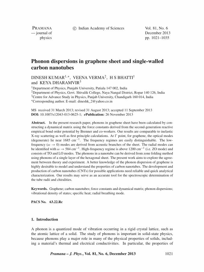
derivative of the energy with respect to stretching and bond bending as shown in figure 1.


Dinesh Kumar et al

B

B

NB

pj k1

pj k2

pij

k2

k1

jiθ

θ

1

2

Figure 1. Bond angles.

A slight change in position of the atom i , k1 or k2 can change the bonding angle whichin turn changes the bonding strength.

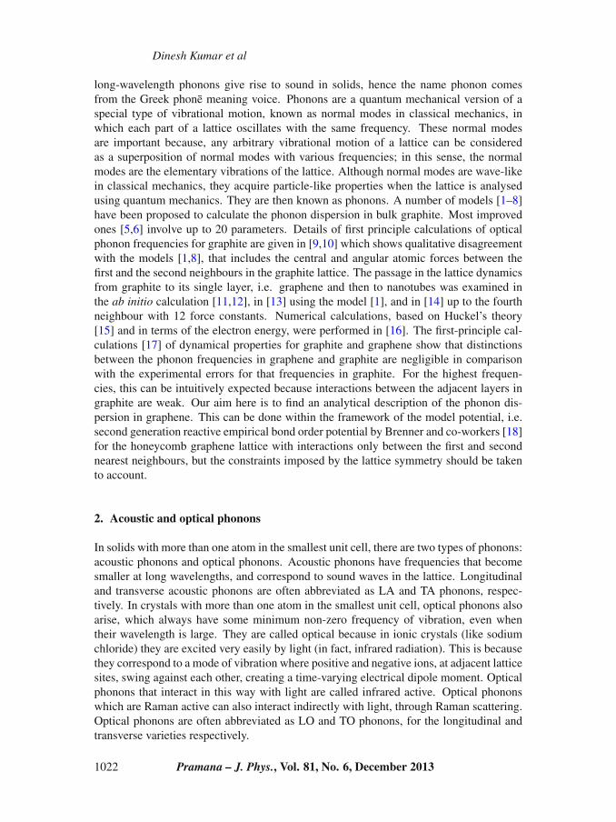
3.2 Description of unit cell and lattice vectors

We consider a two-dimensional sheet of graphene. A part of the generated sheet used forthe calculations is shown in figure 2. The figure shows the hexagonal unit cells as well asthe parallelepipeds defining the crystal lattice, in which the basis consists of two atoms.The lattice vectors are shown with bold arrows. The atomic sites are marked with integers0, 1, 2 etc. and the cells are marked with (0), (1), (2), etc. We shall need only these sixcells for our calculations as all the second neighbours of atoms belonging to the 0th cell

(6)

(5)

(4)

(3)

(2)

(1)r

1

9'

8'

7'

6'9

8

7

6

5

43

2

(0)10

Figure 2. Unit cells in a hexagonal lattice containing C–C atoms.



are contained within these. The lattice vector of cell (1) (connecting the centre of cell (0)to the centre of cell (1)) is shown as an arrow. All the relevant lattice vectors thus obtainedare listed below:

�r1 =(

3b

2

)x +

(√3b

2

)

y,

�r2 = 0x + √3by,

�r3 =(−3b

2

)x +

(√3b

2

)

y,

�r4 = −(

3b

2

)x −

(√3b

2

)

y = −�r1,

�r5 = 0x − √3by = −�r2,

�r6 =(

3b

2

)x −

(√3b

2

)

y = −�r3.

We shall also need to index the atoms differently in order to conform to the notation inφ

mβ j0αi . So the atom with index 0 shown in the diagram, which is of type 1 belonging to

the (0)th cell, must be identified as the 01th atom. Similarly, the atom numbered 1 inthe diagram is the 02th atom in this notation. The conversion between these two types ofnotations is given in Appendix I and is handy in the calculations.

3.3 Construction of a dynamical matrix for graphene sheet

We numerically evaluate the second derivative involving atoms in the central cell goingup to fourth neighbour. In order to evaluate the force constants we use the numericaldifferentiation procedure. We generate a sheet of 31 atoms and obtain the values of ele-ments of dynamical matrix. We do this by evaluating the various energies of this systemwhen either one or two of the atoms are displaced by a small amount , e.g. in expres-sions given in Appendix II, sni denotes the displacement of the nth atom in figure 2 inthe i th direction where i = 1 and 2 mean x and y. Using second-generation reactiveempirical bond order potential, the calculated values of various force constants are givenin Appendix III.

If j �= 3, then φnα j013 = 0. For this reason, the dynamical matrix has a box diagonal

form, with the elements containing the third dimension separated out. For this reasonwe solve only the 6 × 6 matrix corresponding to x–y–z displacements in the sheet.This is described below. Using the force constants obtained, we find the elements ofthe dynamical matrix using eq. (2). The first element D(1, 1) is calculated as below:

D1111 = 1

M1[φ022

011 + ∑K φ J22

011 exp i(�q �ri )]

= D1111 = 1

M1[151.31817 + 2 ∗ 7.56922 ∗ cos(2yy)

− 2 ∗ 1.498 ∗ cos(xx) ∗ cos(yy)],


Dinesh Kumar et al

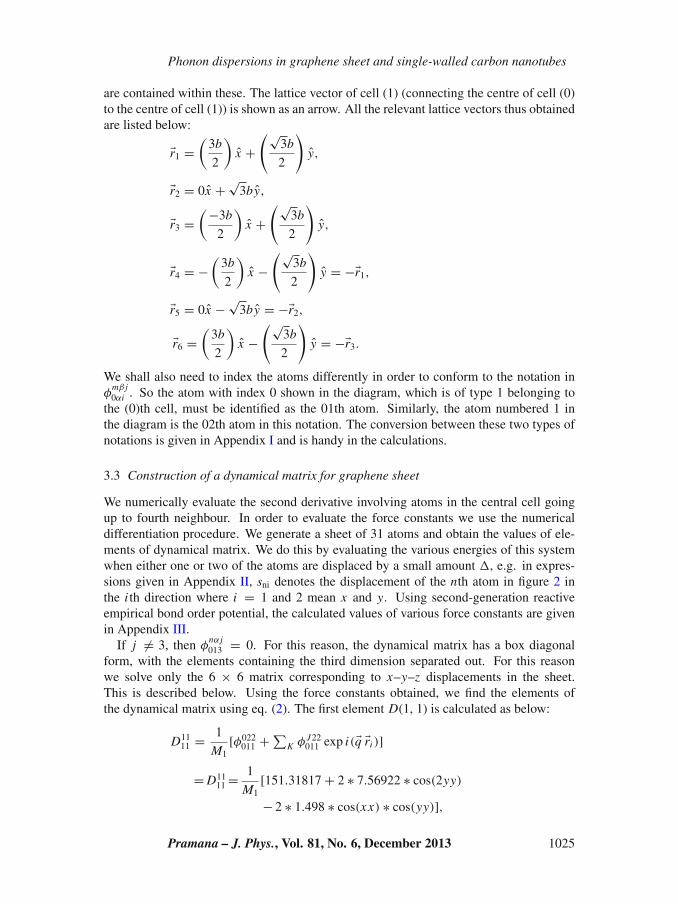
Figure 3. Symmetry points in a single hexagon.

where xx = 3b0qx/2 and yy = √3b0qx/2. Proceeding similarly, we get all the 6 × 6

elements of the dynamical matrix. So eq. (1) now becomes

∣∣∣∣∣∣∣∣∣∣∣∣∣

D1111 − ω2 D12

11 D2111 D22

11

D1112 D12

12 − ω2 D2112 D22

12

D11∗21 D12

21 D2122 − ω2 D22

21

D11∗22 D12∗

22 D2122 D22

22 − ω2

∣∣∣∣∣∣∣∣∣∣∣∣∣

= 0.

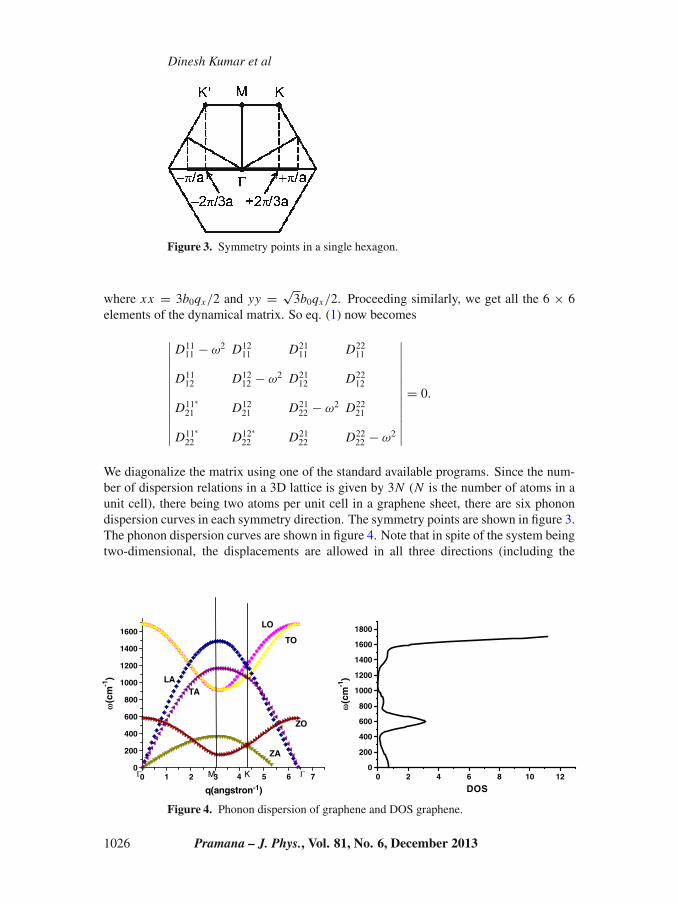
We diagonalize the matrix using one of the standard available programs. Since the num-ber of dispersion relations in a 3D lattice is given by 3N (N is the number of atoms in aunit cell), there being two atoms per unit cell in a graphene sheet, there are six phonondispersion curves in each symmetry direction. The symmetry points are shown in figure 3.The phonon dispersion curves are shown in figure 4. Note that in spite of the system beingtwo-dimensional, the displacements are allowed in all three directions (including the

0 1 2 3 4 5 6 70

200

400

600

800

1000

1200

1400

1600

q(angstron-1)

ω(c

m-1

)

ω(c

m-1

)

ΓΓ M K

LATA

LO

TO

ZO

ZA

0 2 4 6 8 10 120

200

400

600

800

1000

1200

1400

1600

1800

DOS

Figure 4. Phonon dispersion of graphene and DOS graphene.



Table 1. Range of frequency of all branches of graphene.

ωmax(cm−1) ωmin(cm−1)

Branch Graphene Graphene

TO 1685 (1581)a 1068LO 1685, (1583)b, (1582)a 1265LA 1210 0–919 Zero at � pt., (0)a

TA 1210 0–914 Zero at � pt.ZO 584 370ZA 370 0–153 Zero at � pt.

aTheoretical [9].bExperimental [9].

z-direction perpendicular to the plane). Hence there are 3N branches and not 2N . Rangeof frequency of all branches of graphene is shown in table 1.

The phonons in a nanotube can be derived by zone folding method using phonons of asingle layer of the hexagonal sheet.

4. Zone folding method

To calculate the phonon dispersion relation (PDR) and vibrational density of states(VDOS) of CNTs, we adopt the zone folding method which is used for calculating elec-tronic band structure as well as phonons in CNTs. Since the CNT is infinite only in onedimension (say y direction), only qy has quasicontinuous nature. In the x-direction, thetube is obtained by folding the rectangular sheet along the x-direction. For calculatingphonons, the periodicity along x-direction is taken to be the width of the sheet (radiusof the nanotube). Therefore, qx is restricted to only certain values depending on thefinite width. Each line on the phonon dispersion curve represents one of these allowed qx

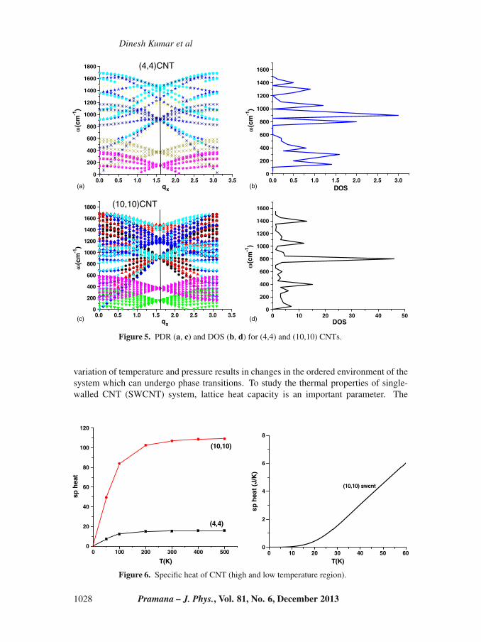
values. We find that there is no real band gap when the sheet is folded into CNT. We cal-culate the PDR and VDOS of the (4,4) and (10,10) CNTs. The results are shown in figure5. Our results are also comparable to Maultzsch et al [9] who measured the dispersion ofthe graphite optical phonons in the in-plane Brillouin zone by inelastic X-ray scatteringas well as first principle calculations.

We also calculate the specific heat of (4,4) and (10,10) CNT and this is depicted infigure 6. As expected, the specific heat of (10,10) CNT approaches a constant value at thehigh temperature limit and a linear T dependence at low temperature.

5. Radial breathing modes in carbon nanotube

For interpreting and understanding theoretical models for studying any system, pressureand temperature dependence of structural and dynamical properties are very useful. The


Dinesh Kumar et al

0.0 0.5 1.0 1.5 2.0 2.5 3.0 0.0 0.5 1.0 1.5 2.0 2.5 3.03.50

200

400

600

800

1000

1200

1400

1600

1800 (4,4)CNT

qx

0.0 0.5 1.0 1.5 2.0 2.5 3.0 3.5qx

0

200

400

600

800

1000

1200

1400

1600

DOS

0

200

400

600

800

1000

1200

1400

1600

1800 (10,10)CNT

0 10 20 30 40 500

200

400

600

800

1000

1200

1400

1600

DOS

ω(c

m-1

)ω

(cm

-1)

ω(c

m-1

)ω

(cm

-1)

(a) (b)

(c) (d)

Figure 5. PDR (a, c) and DOS (b, d) for (4,4) and (10,10) CNTs.

variation of temperature and pressure results in changes in the ordered environment of thesystem which can undergo phase transitions. To study the thermal properties of single-walled CNT (SWCNT) system, lattice heat capacity is an important parameter. The

0 100 200 300 400 5000

20

40

60

80

100

120

(10,10)

(4,4)

sp h

eat

T(K)0 10 20 30 40 50 60

0

2

4

6

8

(10,10) swcnt

sp h

eat

(J/K

)

T(K)

Figure 6. Specific heat of CNT (high and low temperature region).



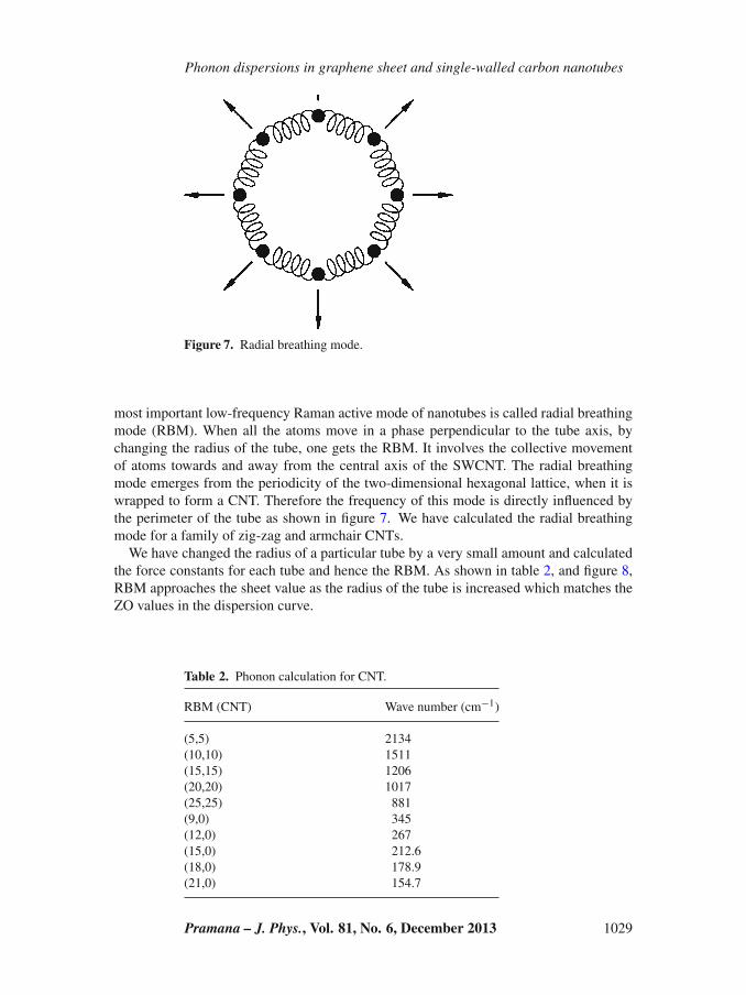
Figure 7. Radial breathing mode.

most important low-frequency Raman active mode of nanotubes is called radial breathingmode (RBM). When all the atoms move in a phase perpendicular to the tube axis, bychanging the radius of the tube, one gets the RBM. It involves the collective movementof atoms towards and away from the central axis of the SWCNT. The radial breathingmode emerges from the periodicity of the two-dimensional hexagonal lattice, when it iswrapped to form a CNT. Therefore the frequency of this mode is directly influenced bythe perimeter of the tube as shown in figure 7. We have calculated the radial breathingmode for a family of zig-zag and armchair CNTs.

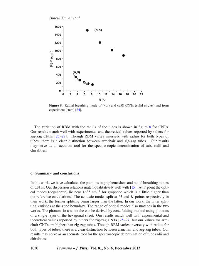
We have changed the radius of a particular tube by a very small amount and calculatedthe force constants for each tube and hence the RBM. As shown in table 2, and figure 8,RBM approaches the sheet value as the radius of the tube is increased which matches theZO values in the dispersion curve.

Table 2. Phonon calculation for CNT.

RBM (CNT) Wave number (cm−1)

(5,5) 2134(10,10) 1511(15,15) 1206(20,20) 1017(25,25) 881(9,0) 345(12,0) 267(15,0) 212.6(18,0) 178.9(21,0) 154.7


Dinesh Kumar et al

0 2 4 6 8 10 12 14 16 18 20 220

200

400

600

800

1000

1200

1400

1600

O

(n,0)

(n,n)

RB

M (

cm-1)

R (A)

Figure 8. Radial breathing mode of (n,n) and (n,0) CNTs (solid circles) and fromexperiment (stars) [24].

The variation of RBM with the radius of the tubes is shown in figure 8 for CNTs.Our results match well with experimental and theoretical values reported by others forzig-zag CNTs [25–27]. Though RBM varies inversely with radius for both types oftubes, there is a clear distinction between armchair and zig-zag tubes. Our resultsmay serve as an accurate tool for the spectroscopic determination of tube radii andchiralities.

6. Summary and conclusions

In this work, we have calculated the phonons in graphene sheet and radial breathing modesof CNTs. Our dispersion relations match qualitatively well with [15]. At � point the opti-cal modes (degenerate) lie near 1685 cm−1 for graphene which is a little higher thanthe reference calculations. The acoustic modes split at M and K points respectively intheir work, the former splitting being larger than the latter. In our work, the latter split-ting vanishes at the zone boundary. The range of optical modes also matches in the twoworks. The phonons in a nanotube can be derived by zone folding method using phononsof a single layer of the hexagonal sheet. Our results match well with experimental andtheoretical values reported by others for zig-zag CNTs [25–27] but our values for arm-chair CNTs are higher than zig-zag tubes. Though RBM varies inversely with radius forboth types of tubes, there is a clear distinction between armchair and zig-zag tubes. Ourresults may serve as an accurate tool for the spectroscopic determination of tube radii andchiralities.



Appendix I

Table A. Indices of the site of some of atoms

Index Index for Index for thefor atom the hexagon cell type of atom

0 0 11 0 22 3 23 4 24 6 15 1 16 2 17 3 18 4 19 5 16′ 5 27′ 6 28′ 1 29′ 2 2

Appendix II. Numerical differentiation procedure for evaluating force constants

∂2φ

∂s01∂s11= ∂

∂01

∂φ

∂s11

= 1

2

[(∂φ

∂s11

)

x0=x

−(

∂φ

∂s01

)

x0=−

]

= 1

42

[(φ(x1 = ) − φ(x1 = −))x0=

− (φ(x1 = ) − φ(x1 = −))x0=−

]

= 1

42[φ(x0 =, x1 =) − φ(x0 =, x1 =−)

−φ(x0 =−, x1 =) + φ(x0 =−, x1 =−)]

= 1

42[2φ(x0 = , x1 = ) − φ(x0 = , x1 = −)

−φ(x0 = −, x1 = )] , (5)

∂2φ

∂s01∂s12= 0 = ∂2φ

δs02∂s11, (6)

∂2φ

∂s02∂s12= 1

22

[φ(y0 = , y1 = ) − φ(y0 = , y1 = −)

], (7)


Dinesh Kumar et al

∂2φ

∂s201

= 1

2[φ(x0 = ) + φ(x0 = −) − 2φ0] , (8)

∂2φ

∂s202

= 2

2

[φ(y0 = −) − φ0

]. (9)

There are two non-vanishing terms only. Other terms are zero. We can find derivativesbetween 0 and 2 and 0 and 3 by the transformation of x and y as shown below. Choosingthe primed coordinate system, x ′ from atom 0 to atom 2 and y′ normal to it, we obtain

∣∣∣∣x ′y′

∣∣∣∣ =∣∣∣∣

cos 120◦ − sin 120◦sin 120◦ cos 120◦

∣∣∣∣

∣∣∣∣xy

∣∣∣∣ ,

where

x ′ = x

2−

√3

2y, (10)

y′ =√

3

2x − y

2, (11)

∂2φ

∂s01∂s11= ∂2φ

∂s01′∂s11′, (12)

∂φ

∂s21= ∂φ

∂s21′∂s21′

∂s21+ ∂φ

∂s22′

∂s22′

∂s22

= −1

2

∂φ

∂s21′− 1

2

∂φ

∂s22′, (13)

∂2φ

∂s01∂s21= −1

2

∂

∂s01

∂φ

∂s21′− 1

2

∂

∂s01

∂φ

∂s22′

= − 1

2

∂

∂s01′

∂φ

∂s21′

(∂s01

∂s01

)− 1

2

∂

∂s02′

∂φ

∂s21′

(∂s02′

∂s01

)

− 1

2

∂

∂s01′

∂φ

∂s22′

(∂s01′

∂s01

)− 1

2

∂

∂s02′

∂φ

∂s22′

(∂s02′

∂s01

)

−1

4

∂2φ

∂s01′∂s21′

√3

4

∂2φ

∂s02′∂s22′

= 1

4

∂2φ

∂s01∂s11

√3

4

∂2φ

∂s02∂s12. (14)



Going along the same lines, the general method to extract second derivative in rotatedcoordinate system is given by

∂2φ

∂s0i∂s2 j= ∂

∂s0i

∂φ

∂s2 j= ∂s0i ′

∂s0i

∂

∂s02′

(∂φ

∂s2 j

)+ ∂s0other′

∂s0i

∂

∂s0other′

(∂φ

∂s2 j

)

=2∑

i ′=1

∂s0i ′

∂s0i

∂

∂s0i ′

(∂φ

∂s2 j

)=

2∑

i ′=1

∂si ′

∂si

∂

∂s0i ′

2∑

j ′=1

∂s2 j ′

∂s2 j

(∂φ

∂s2 j ′

)

=2∑

i ′=1

2∑

j ′=1

(∂si ′

∂si

) (∂s j ′

∂s j

) (∂2φ

∂s01′∂s2 j ′

). (15)

Since there are only φ1101 and φ12

02 as non-vanishing array φ1 j0i elements, we have

φ2101 = ∂x ′

∂x

∂x ′

∂xφ11

01 + ∂y′

∂x

∂y′

∂xφ12

02 = 1

4φ11

01 + 3

4φ12

02 , (16)

φ2101 = 1

4φ11

01 + 3

4φ12

02 , (17)

φ2201 =

√3

4φ11

01 −√

3

4φ12

02 , (18)

φ2102 =

√3

4φ11

01 −√

3

4φ12

02 , (19)

φ2202 = −3

4φ11

01 + 1

4φ12

02 . (20)

For site 3, we rotate x and y by −120◦ and

x ′ = − x

2+

√3

2y, (21)

y′ = −√

3

2x − y

2. (22)

In the same manner we get the other equations by replacing 2 by 3.

Appendix III. Force constants for graphene

φ011011 = φ012

012 = φ021021 = φ022

022 = 151.312 eV/Å−2, (23)

φ022012 = −65.322 eV/Å−2, (24)


Dinesh Kumar et al

φ021011 = φ011

021 = −41.654 eV/Å−2, (25)

φ111011 = φ311

011 = φ411011 = φ611

011 = −1.498 eV/Å−2, (26)

φ011021 = φ012

011 = φ012021 = φ011

022 = 0, (27)

φ311012 = φ612

011 = −0.865 eV/Å−2, (28)

φ112011 = φ412

012 = 0.865 eV/Å−2, (29)

φ611012 = φ312

011 = 11.334 eV/Å−2, (30)

φ111012 = φ412

011 = −11.334 eV/Å−2, (31)

φ112012 = φ312

012 = φ412012 = φ612

012 = 4.547 eV/Å−2, (32)

φ211011 = φ511

011 = 7.569 eV/Å−2, (33)

φ212011 = φ511

012 = −6.099 eV/Å−2, (34)

φ512011 = φ211

012 = 6.099 eV/Å−2, (35)

φ212012 = φ512

012 = −4.520 eV/Å−2, (36)

φ321011 = φ421

011 = −59.405 eV/Å−2, (37)

φ322011 = φ321

012 = −10.249 eV/Å−2, (38)

φ422011 = φ421

012 = 10.249 eV/Å−2, (39)

φ322012 = φ422

012 = −47.571 eV/Å−2. (40)

We have calculated the force constants along z-direction also but the values arecomparatively lower than the force constants along x-direction and y-direction.

φ013013 = φ023

023 = 11.596 eV/Å−2, (41)

φ023013 = φ323

013 = φ423013 = −6.409 eV/Å−2, (42)

φ113013 = φ213

013 = φ313013 = φ413

013 = φ513013 = φ613

013 = φ423013 = 1.272 eV/Å−2. (43)



References

[1] J De Launay, Solid State Phys. 3, 203 (1957)[2] R Nicklow, W Wakabayashi and H G Smith, Phys. Rev. B 5, 4951 (1972)[3] A A Ahmadieh and H A Rafizadeh, Phys. Rev. B 7, 4527 (1973)[4] A P P Nicholson and D J Bacon, J. Phys. C 10, 2295 (1977)[5] M Maeda, Y Kuramoto and C Horie, J. Phys. Soc. Jpn. Lett. 47, 337 (1979)[6] R Al-Jishi and G Dresselhaus, Phys. Rev. B 26, 4514 (1982)[7] H Gupta, J Malhotra, N Rani and B Tripathi, Phys. Rev. B 33, 7285 (1986)[8] L Lang, S Doyen-Lang, A Charlier and M F Charlier, Phys. Rev. B 49, 5672 (1994)[9] J Maultzsch, S Reich, C Thomsen, H Reequardt and P Ordejon, Phys. Rev. Lett. 92, 075501

(2004)[10] M Mohr, J Maultzsch, E Dobardzic, I Milosevic, M Damnjanovic, A Bosak, M Krish and

C Thomsen, Phys. Rev. B 76, 035439 (2007)[11] D Sánchez-Portal, E Artacho and J M Soler, Phys. Rev. B 59, 12678 (1999)[12] O Dubay and G Kresse, Phys. Rev. B 67, 035401 (2003)[13] A Charlier, E McRae, M-F Charlier, A Spire and S Forster, Phys. Rev. B 57, 6689 (1998)[14] A Gruneis, R Saito, T Kimura, L G Cancado, M A Primenta, A Jorio, A G Souza Filho,

G Dresselhaus and M S Dresselhaus, Phys. Rev. B 65, 155405 (2002)[15] C Mapelli, C Castiglioni and G Zerbi, Phys. Rev. B 60, 12710 (1999)[16] V N Popov and P Lambin, Phys. Rev. B 73, 085407 (2006)[17] N Mounet and N Marzari, Phys. Rev. B 71, 205214 (2005)[18] D W Brenner, O A Shenderova, J A Harrison, S J Stuart, B Ni and S B Sinnott, J. Phys.:

Condens. Matter 14, 783 (2002)[19] D Goldberg, Y Bando, L Bourgeois, K Kurashima and T Sato, Appl. Phys. Lett. 77, 13 (2000)[20] R Ma, Y Bando and T Sato, Adv. Mater. 14, 366 (2002)[21] D Kumar, V Verma, H S Bhatti and K Dharamvir, J. Nanomater. 2011, Article ID 127952,

6 pages, 2011, DOI: 10.1155/2011/127952[22] D Kumar, V Verma and K Dharamvir, J. Nano Res. 15, 1 (2011)[23] D Kumar, V Verma, K Dharamvir and H S Bhatti, AIP Proceedings 1393, 207 (2011)[24] S Reich, A C Ferrari, R Arenal, A Loiseau, I Bello and J Robertson, Phys. Rev. B 71, 205201

(2005)[25] J Q Lu, T E Kopley, N Moll, D Roitman, D Chamberlin, Q Fu, J Liu, T P Russell, D A Rider,

I Manners and M A Winnik, Chem. Mater. 17, 2227 (2005)[26] P Saxena and S P Sanyal, Pramana – J. Phys. 67, 305 (2006)[27] V N Popov, V E Van Doren and M Balkanski, Phys. Rev. B 59, 8355 (1999)


http://dx.doi.org/10.1155/2011/127952

phonon dispersions in graphene sheet and single-walled

Documents