physical optics 3 diffraction, resolution and image
TRANSCRIPT

www.iap.uni-jena.de
Physical Optics
Lecture 3 : Diffraction, resolution and Fourier Optics
2017-04-19
Beate Boehme

Physical Optics: Content2
No Date Subject Ref Detailed Content
1 05.04. Wave optics G Complex fields, wave equation, k-vectors, interference, light propagation, interferometry
2 12.04. Diffraction B Slit, grating, diffraction integral, diffraction in optical systems, point spread function, aberrations
3 19.04. Fourier optics B Plane wave expansion, resolution, image formation, transfer function, phase imaging
4 26.04. Quality criteria and resolution B Rayleigh and Marechal criteria, Strehl ratio, coherence effects, two-
point resolution, criteria, contrast, axial resolution, CTF
5 03.05. Polarization G Introduction, Jones formalism, Fresnel formulas, birefringence, components
6 10.05. Photon optics D Energy, momentum, time-energy uncertainty, photon statistics, fluorescence, Jablonski diagram, lifetime, quantum yield, FRET
7 17.05. Coherence G Temporal and spatial coherence, Young setup, propagation of coherence, speckle, OCT-principle
8 24.05. Laser B Atomic transitions, principle, resonators, modes, laser types, Q-switch, pulses, power
9 31.05. Gaussian beams D Basic description, propagation through optical systems, aberrations
10 07.06. Generalized beams D Laguerre-Gaussian beams, phase singularities, Bessel beams, Airy beams, applications in superresolution microscopy
11 14.06. PSF engineering G Apodization, superresolution, extended depth of focus, particle trapping, confocal PSF
12 21.06. Nonlinear optics D Basics of nonlinear optics, optical susceptibility, 2nd and 3rd order effects, CARS microscopy, 2 photon imaging
13 28.06. Scattering G Introduction, surface scattering in systems, volume scattering models, calculation schemes, tissue models, Mie Scattering
14 05.07. Miscellaneous G Coatings, diffractive optics, fibers
D = Dienerowitz B = Böhme G = Gross
Diffraction at slit
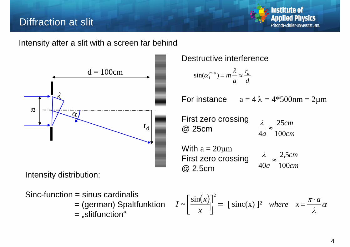
Intensity after a slit with a screen far behind a
Destructive interference
dr
am d )sin( min
1
4
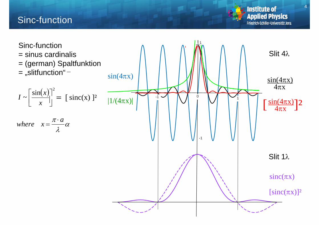
2sin~
xxI
axwhere
sinc(x) ]²
Intensity distribution:
Sinc-function = sinus cardinalis= (german) Spaltfunktion= „slitfunction“
For instance a = 4 = 4*500nm = 2µm
First zero crossing@ 25cm
With a = 20µm First zero crossing@ 2,5cm
d = 100cm
rdcmcm
a 10025
4
cmcm
a 1005,2
40
4
-1
sin(4x)
|1/(4x)|
sin(4x)4x
-1 10
1
sin(4x)4x[ ]²
2sin~
xxI
axwhere
sinc(x) ]²
Sinc-function= sinus cardinalis= (german) Spaltfunktion= „slitfunction“
Sinc-function
sinc(x)
[sinc(x)]²
Slit 4
Slit 1
5
Diffraction at slit
-2 -1 0 1
0
1
-2 -1 0 1 20
1
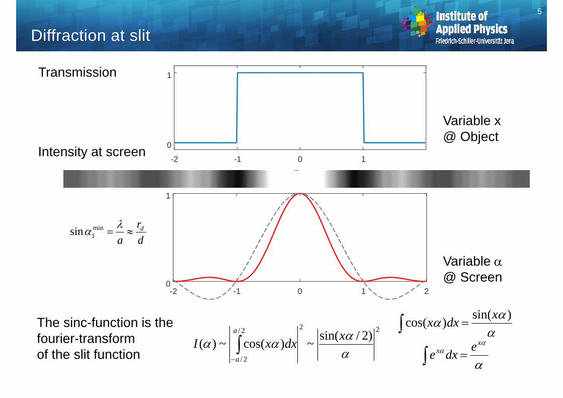
Transmission
Intensity at screen
)sin()cos( xdxx The sinc-function is the
fourier-transformof the slit function
222/
2/
)2/sin(~)cos(~)( xdxxI
a
a
xx edxe
Variable x@ Object
Variable @ Screen
dr
ad
min1sin
6
Diffraction at circular aperture
-2 -1 0 1
0
1
-2 -1 0 1 20
1
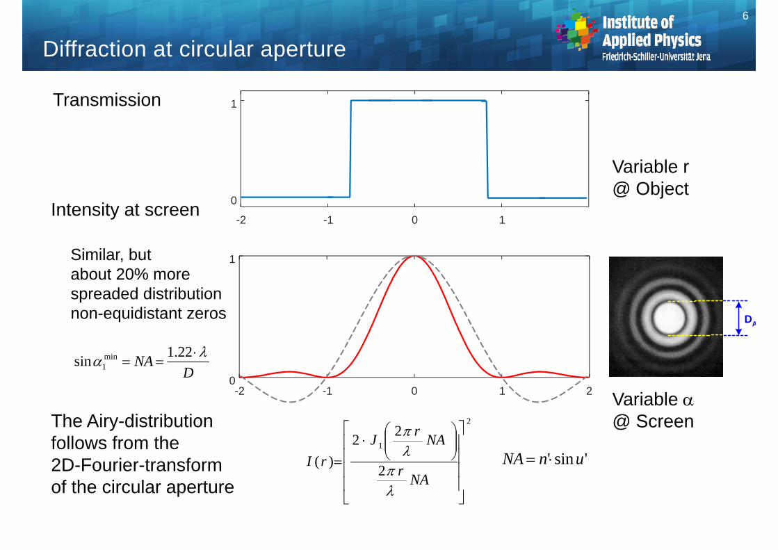
Transmission
Intensity at screen
The Airy-distribution follows from the2D-Fourier-transform of the circular aperture
Variable r@ Object
Variable @ Screen
DA
DNA
22.1sin min
1
'sin' unNA
2
1
2
22)(
NAr
NArJrI
Similar, but about 20% morespreaded distributionnon-equidistant zeros

Fourier Transformation 7
Corresponds to the description of a function as sum of sine or cosine-functions:
Real numbers: sinus and cosine transformation
Description of a (periodic) function as sum of cosine- or sine-functions
Complex formulation: Fourier transformation (FFT)
Corresponds to principle of superposition of electric fields
~ cos
~ sin
~ cos
~
8
Fourier Transformation
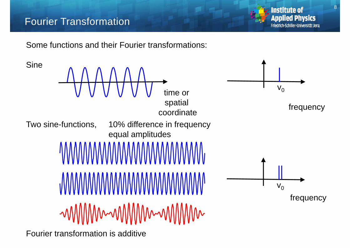
Some functions and their Fourier transformations:
Sine
Two sine-functions, 10% difference in frequencyequal amplitudes
Fourier transformation is additive
time or spatial
coordinatefrequency
v0
frequencyv0

9
Fourier Transformation
Some functions (signals) and their Fourier transformations (spectra):
Uniform, constant function
pulse vica versa
Gaussian function exp(- a t ²)
Exponential exp( - | t |)
x frequency
vv0x
delta-function@ v = 0
Uniform spectrum
Gauss
Lorentz very slow . 2 . decrease
[ 1+ (2pv)²]
10
Fourier Transformation
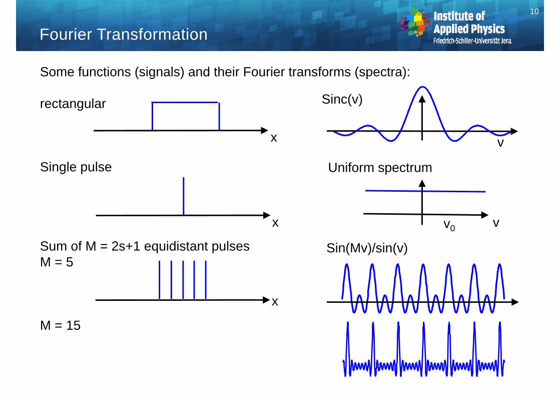
Some functions (signals) and their Fourier transforms (spectra):
rectangular
Single pulse
Sum of M = 2s+1 equidistant pulsesM = 5
M = 15
x
vv0x
Sinc(v)
Uniform spectrum
Sin(Mv)/sin(v)
v
x
11
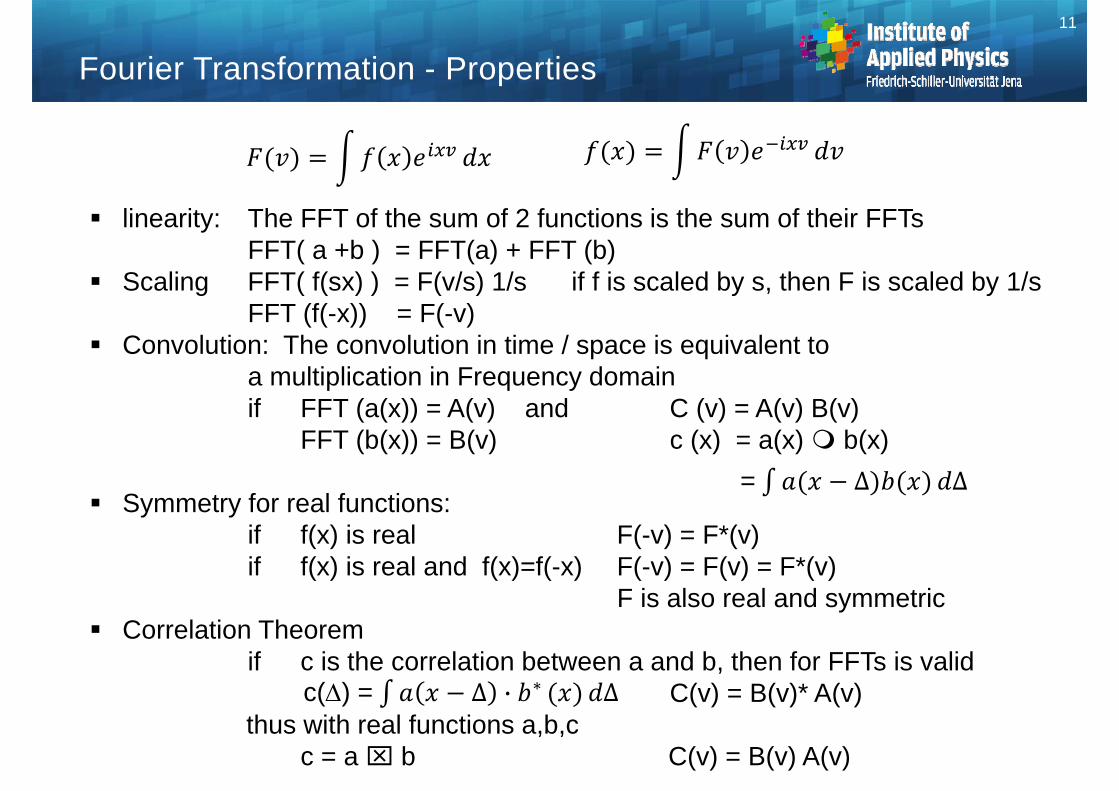
Fourier Transformation - Properties
linearity: The FFT of the sum of 2 functions is the sum of their FFTsFFT( a +b ) = FFT(a) + FFT (b)
Scaling FFT( f(sx) ) = F(v/s) 1/s if f is scaled by s, then F is scaled by 1/sFFT (f(-x)) = F(-v)
Convolution: The convolution in time / space is equivalent to a multiplication in Frequency domainif FFT (a(x)) = A(v) and C (v) = A(v) B(v)
FFT (b(x)) = B(v) c (x) = a(x) b(x)
Symmetry for real functions: if f(x) is real F(-v) = F*(v) if f(x) is real and f(x)=f(-x) F(-v) = F(v) = F*(v)
F is also real and symmetric Correlation Theorem
if c is the correlation between a and b, then for FFTs is validC(v) = B(v)* A(v)
thus with real functions a,b,cc = a b C(v) = B(v) A(v)
= Δ Δ
c() = Δ · ∗ Δ

Fourier-Theory - Diffraction at sinus-grating 12
x vv0
x v
Sinusoidal transmission
Plus offset
= transmission function
Due to symmetry for real, symmetric function the orders 0, +1 and -1 occur
Limited extension of grating corresponds to multiplication with rectangle function no ideal delta-functions,
but broadening corresponding to Airy
v
13
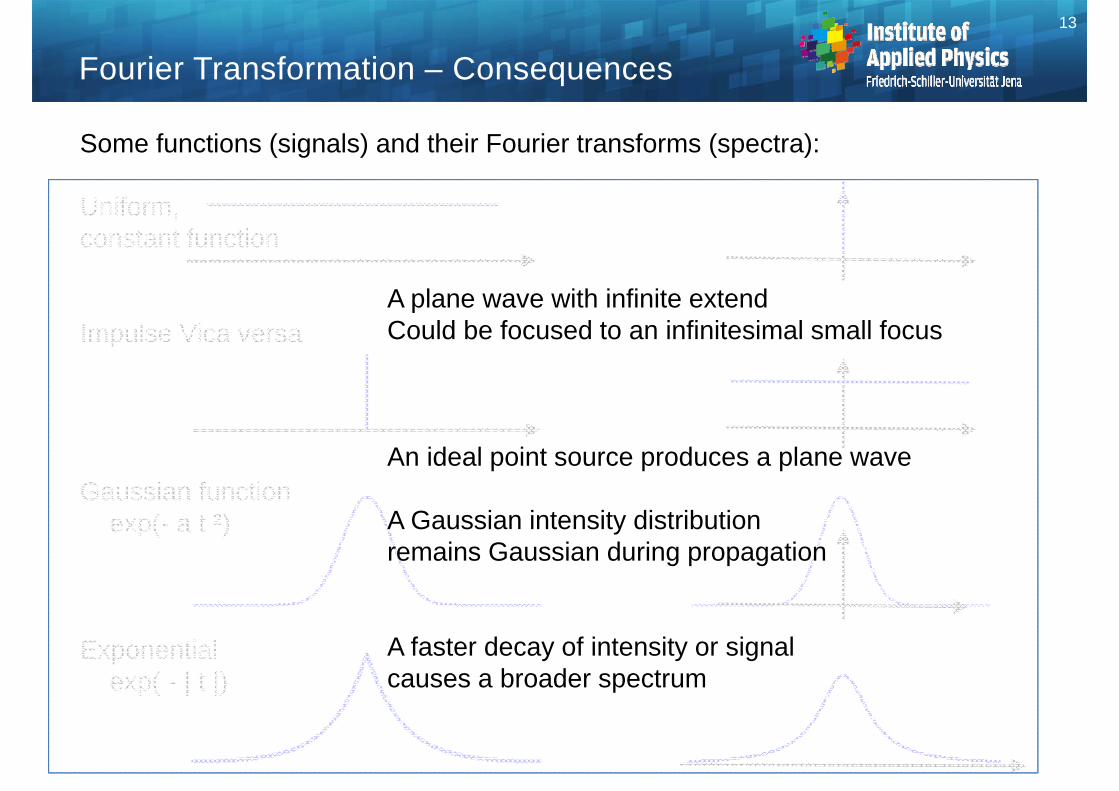
Fourier Transformation – Consequences
Some functions (signals) and their Fourier transforms (spectra):
Uniform, constant function
Impulse Vica versa
Gaussian function exp(- a t ²)
Exponential exp( - | t |)
A plane wave with infinite extend Could be focused to an infinitesimal small focus
An ideal point source produces a plane wave
A Gaussian intensity distributionremains Gaussian during propagation
A faster decay of intensity or signal causes a broader spectrum
14
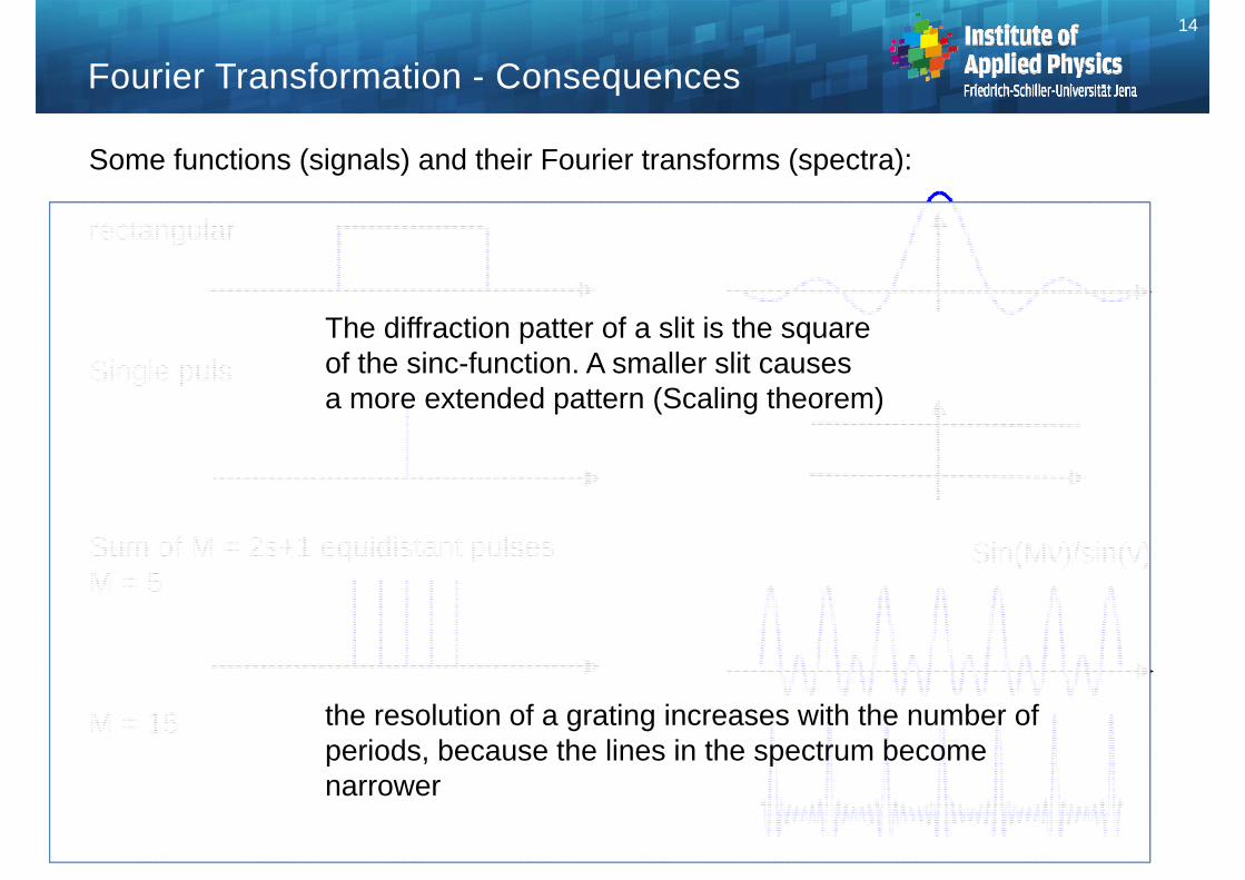
Fourier Transformation - Consequences
Some functions (signals) and their Fourier transforms (spectra):
rectangular
Single puls
Sum of M = 2s+1 equidistant pulsesM = 5
M = 15
Sin(Mv)/sin(v)
The diffraction patter of a slit is the square of the sinc-function. A smaller slit causes a more extended pattern (Scaling theorem)
the resolution of a grating increases with the number of periods, because the lines in the spectrum become narrower
15
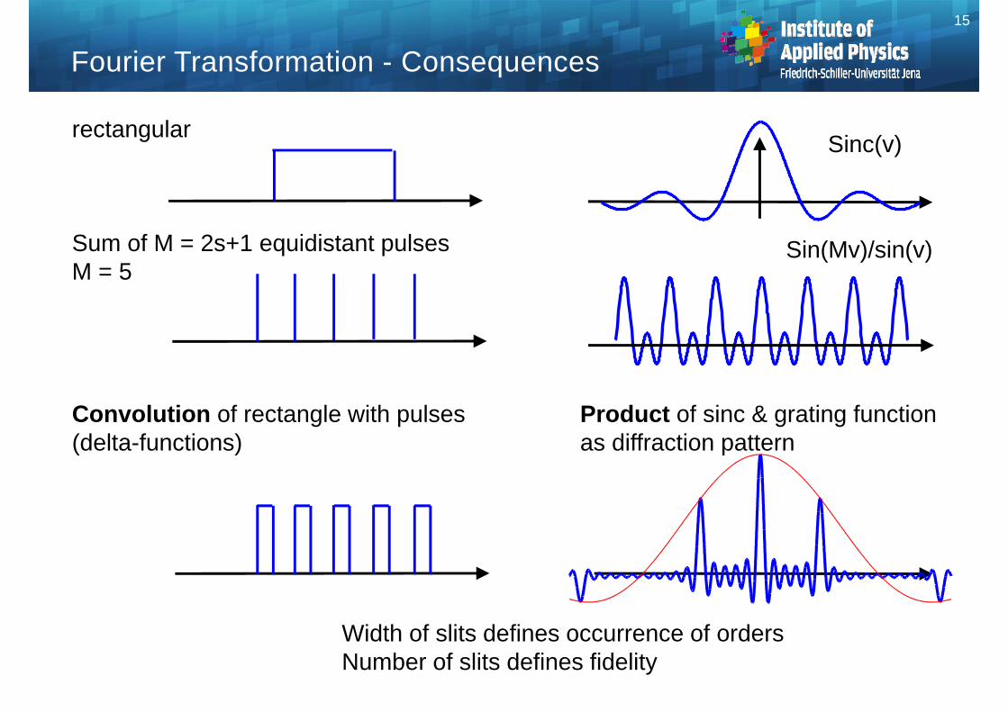
Fourier Transformation - Consequences
rectangular
Sum of M = 2s+1 equidistant pulsesM = 5
Convolution of rectangle with pulses Product of sinc & grating function (delta-functions) as diffraction pattern
Sin(Mv)/sin(v)
Width of slits defines occurrence of ordersNumber of slits defines fidelity
Sinc(v)

Diffraction at grating – Complex Field 16
1. Width of slits defines occurrence of orders
2. Number of slits defines fidelity
3. Period of grating defines distance of orders
1-2-3-4 1-2-3-45 5
Between the maxima are 5 periods –The number increases with number of periods M
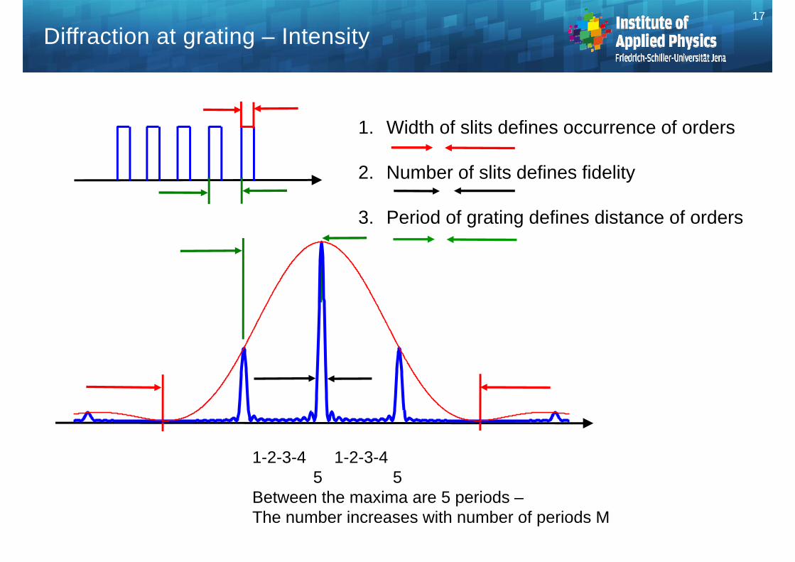
Diffraction at grating – Intensity 17
1. Width of slits defines occurrence of orders
2. Number of slits defines fidelity
3. Period of grating defines distance of orders
1-2-3-4 1-2-3-45 5
Between the maxima are 5 periods –The number increases with number of periods M
18
-2 -1 0 1 20
0.5
1
-2 -1 0 1 2-1
0
1
-2 -1 0 1 2-0.5
0
0.5
-2 -1 0 1 2-1
0
1
-2 -1 0 1 2-0.5
0
0.5
-2 -1 0 1 2-1
0
1
-2 -1 0 1 2-0.5
0
0.5
-2 -1 0 1 2-1
0
1
-2 -1 0 1 2-0.5
0
0.5
-2 -1 0 1 2-1
0
1
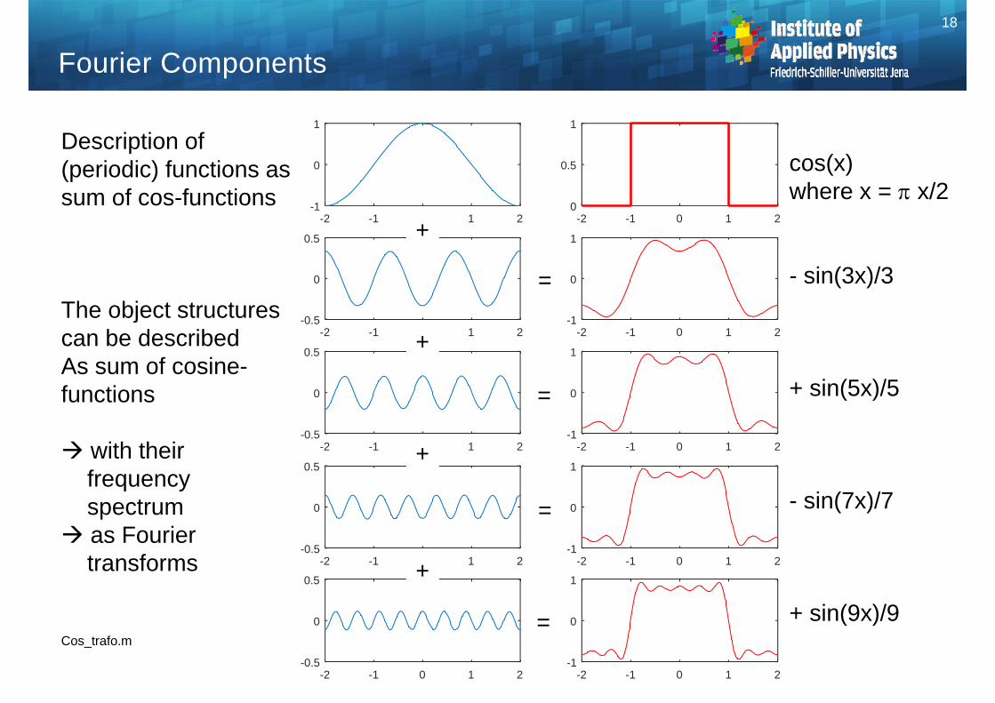
Description of (periodic) functions as sum of cos-functions
The object structures can be described As sum of cosine-functions
with their frequency spectrum
as Fourier transforms
Cos_trafo.m
=
=
=
=
+
+
+
+
cos(x) where x = x/2
- sin(3x)/3
+ sin(5x)/5
- sin(7x)/7
+ sin(9x)/9
Fourier Components
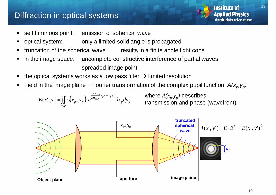
Diffraction in optical systems
self luminous point: emission of spherical wave optical system: only a limited solid angle is propagated truncation of the spherical wave results in a finite angle light cone in the image space: uncomplete constructive interference of partial waves
spreaded image point the optical systems works as a low pass filter limited resolution Field in the image plane ~ Fourier transformation of the complex pupil function A(xp,yp)
19
Object plane aperture image plane
truncatedspherical
wavexp, yp
pp
yyxxR
i
ppExP
dydxeyxAyxEpp
ExP''2
,)','(
where A(xp,yp) describes
transmission and phase (wavefront)
2* )','()','( yxEEEyxI
DAiry
19
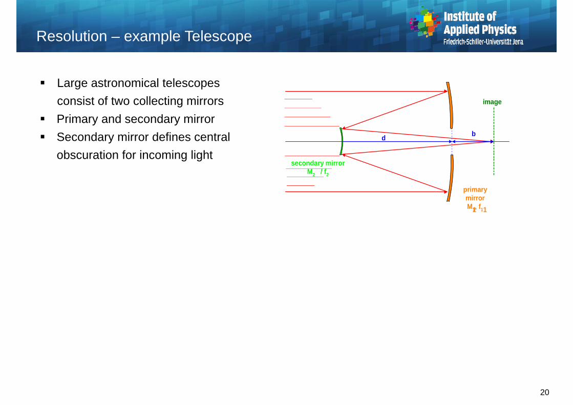
Large astronomical telescopes consist of two collecting mirrors
Primary and secondary mirror Secondary mirror defines central
obscuration for incoming light secondary mirror
M2 / f2
primarymirrorM1, f1
image
bd
11
Resolution – example Telescope
20
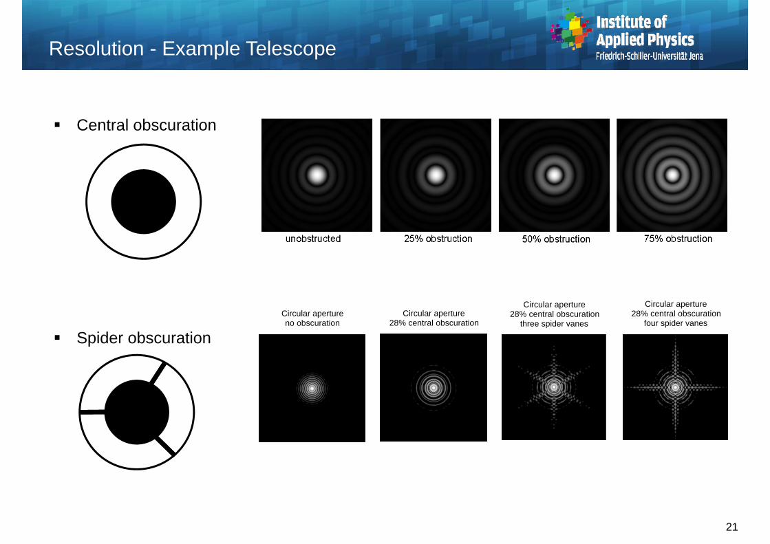
Central obscuration
Spider obscuration
Circular apertureno obscuration
Circular aperture28% central obscuration
Circular aperture28% central obscuration
three spider vanes
Circular aperture28% central obscuration
four spider vanes
Resolution - Example Telescope
21
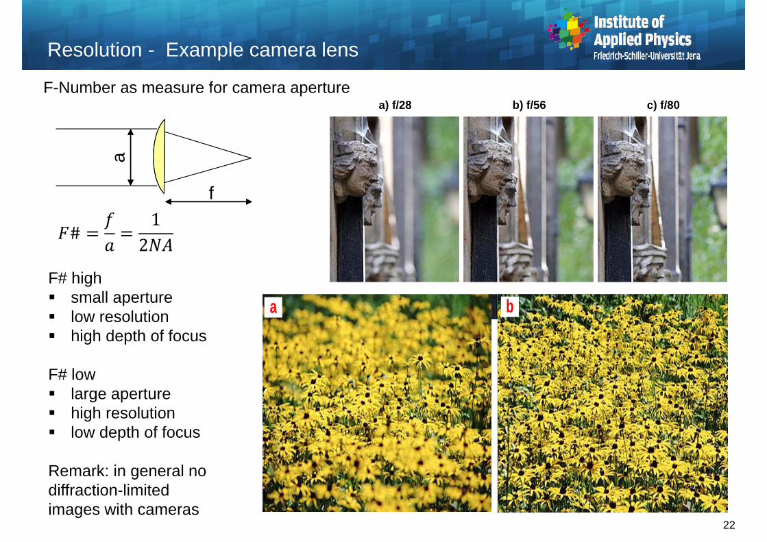
a) f/28 b) f/56 c) f/80
Resolution - Example camera lens
22
F-Number as measure for camera aperture
#1
2
F# high small aperture low resolution high depth of focus
F# low large aperture high resolution low depth of focus
Remark: in general no diffraction-limited images with cameras
a
f
a b
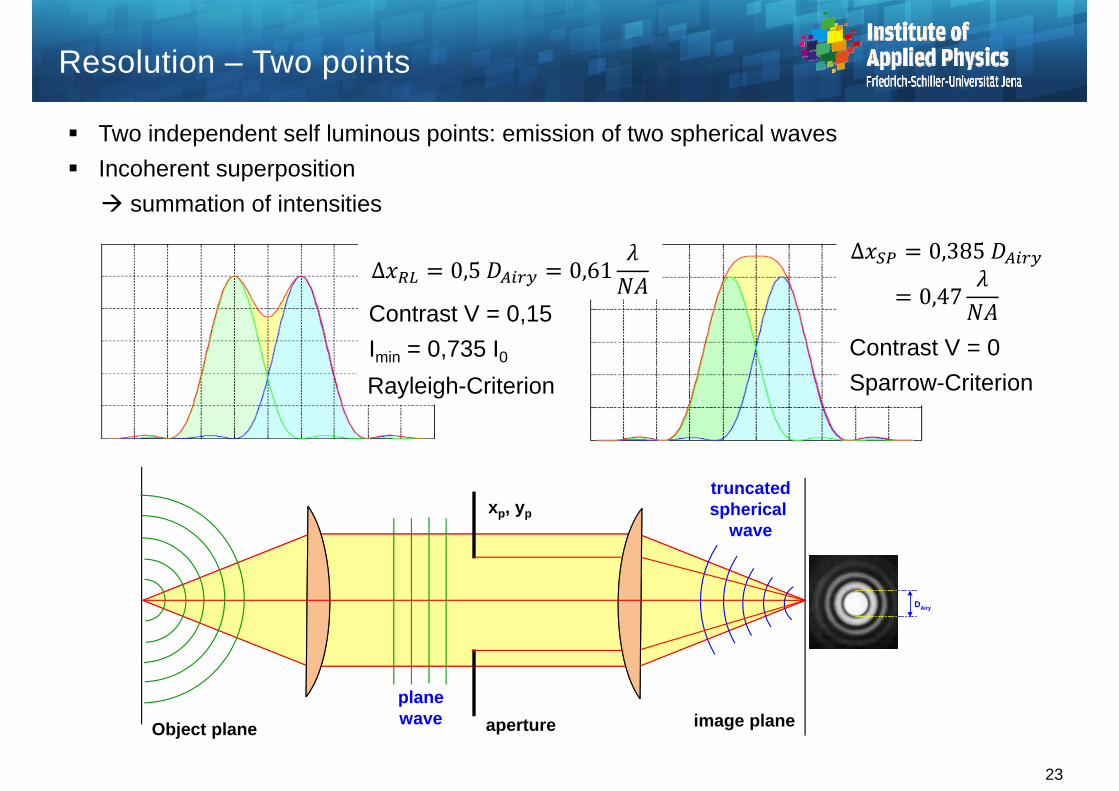
Resolution – Two points
Two independent self luminous points: emission of two spherical waves Incoherent superposition summation of intensities
23
Object plane aperture image plane
truncatedspherical
wavexp, yp
DAiry
Δ 0,5 0,61Δ 0,385
0,47Contrast V = 0,15Imin = 0,735 I0 Contrast V = 0
Sparrow-CriterionRayleigh-Criterion
planewave

24
Resolution – Two points
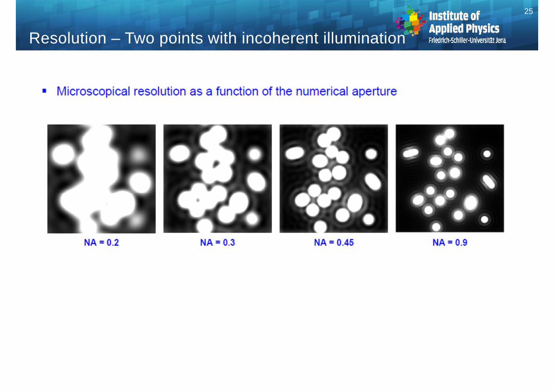
25
Resolution – Two points with incoherent illumination
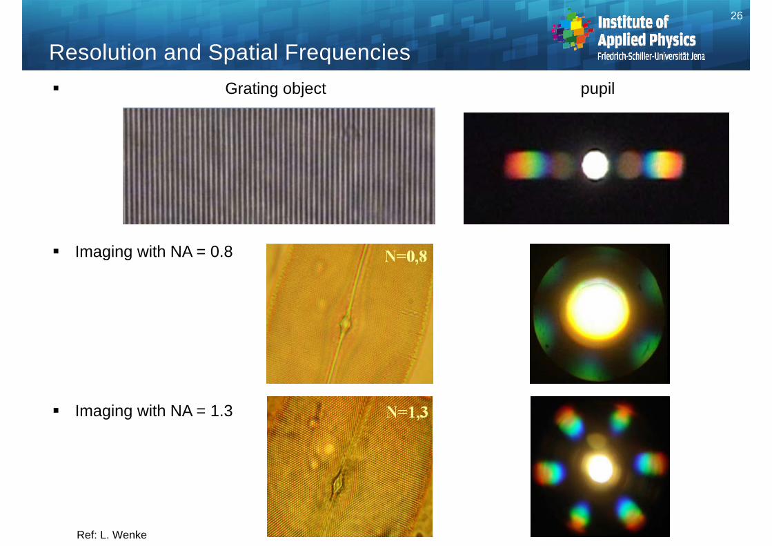
Resolution and Spatial Frequencies Grating object pupil
Imaging with NA = 0.8
Imaging with NA = 1.3
Ref: L. Wenke
26

Resolution – More incoherent points
more independent self luminous points: emission of N spherical waves summation of intensities First point (green)
27
Object planeaperture image plane
truncatedspherical
wavexp, yp
DAiry
planewave
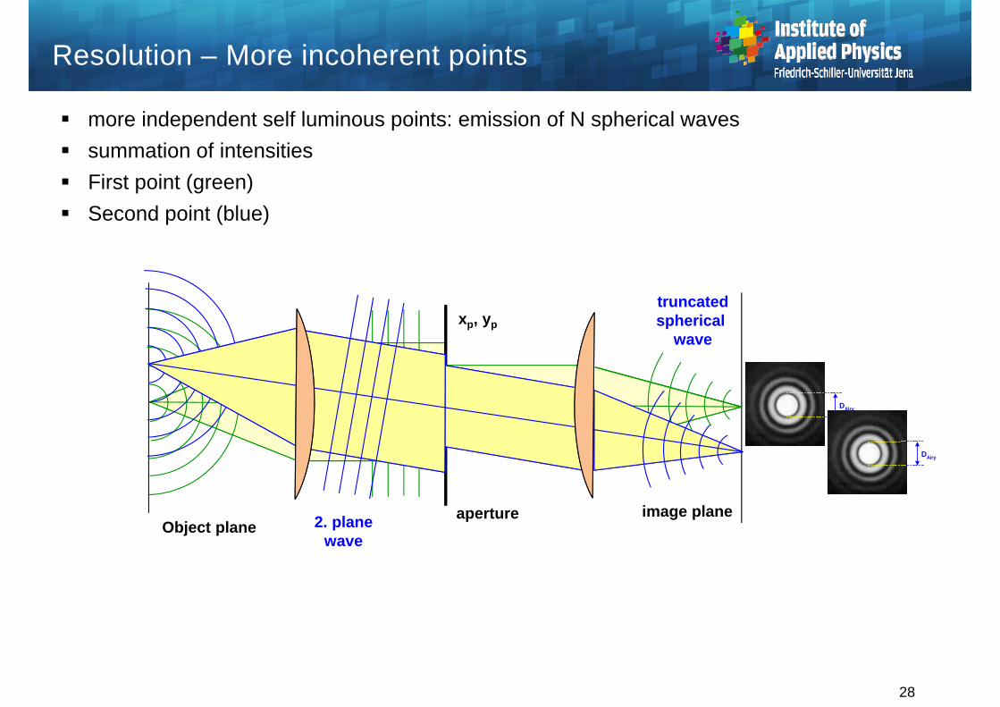
Resolution – More incoherent points
more independent self luminous points: emission of N spherical waves summation of intensities First point (green) Second point (blue)
28
Object planeaperture image plane
truncatedspherical
wavexp, yp
DAiry
2. planewave
DAiry
Resolution – More incoherent points
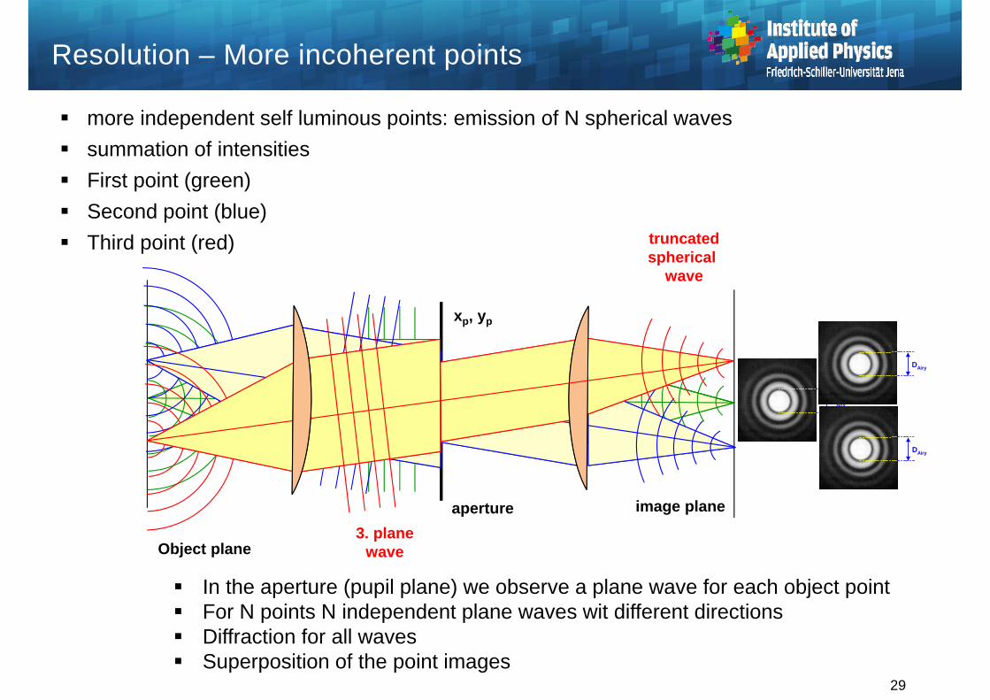
more independent self luminous points: emission of N spherical waves summation of intensities First point (green) Second point (blue) Third point (red)
29
Object plane
aperture image plane
truncatedspherical
wave
xp, yp
DAiry
3. planewave
DAiry
DAiry
In the aperture (pupil plane) we observe a plane wave for each object point For N points N independent plane waves wit different directions Diffraction for all waves Superposition of the point images

Incoherent points in image plane
Superposition of image intensities
30
image plane
truncatedspherical
wave
DAiry
DAiry
DAiry
-10
1

Overlay of point images31
1
-1 0 1
0
-1 0 1
0
1
-1 0 1
0
1
-1 0 1
Visibility = Contrast:
Imax=1
Imin=0
V = 1
Imax=1
Imin=0.735
V = (1-0.735)/(1+0.735)V = 0.15
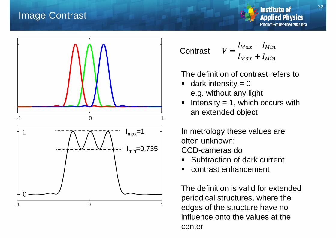
Image Contrast32
-1 0 1
0
1
-1 0 1
Contrast
Imax=1
Imin=0.735
The definition of contrast refers to dark intensity = 0
e.g. without any light Intensity = 1, which occurs with
an extended object
In metrology these values are often unknown: CCD-cameras do Subtraction of dark current contrast enhancement
The definition is valid for extended periodical structures, where the edges of the structure have no influence onto the values at the center

Resolution – Vice Versa discusssion
Plane waves with different directions in the object plane Focused, convergent waves in the pupil plane Coordinate of focus depends on direction of plane wave Limitation of directions by the aperture Superposition of the transmitted plane waves in the image
Plane waves can be thought of generated by a grating, illuminated with a plane wave Far field diffraction pattern in the pupil
33
Object plane
apertureimage plane
xp, yp
plane wavesuperposition
Resolution – Vice Versa discusssion
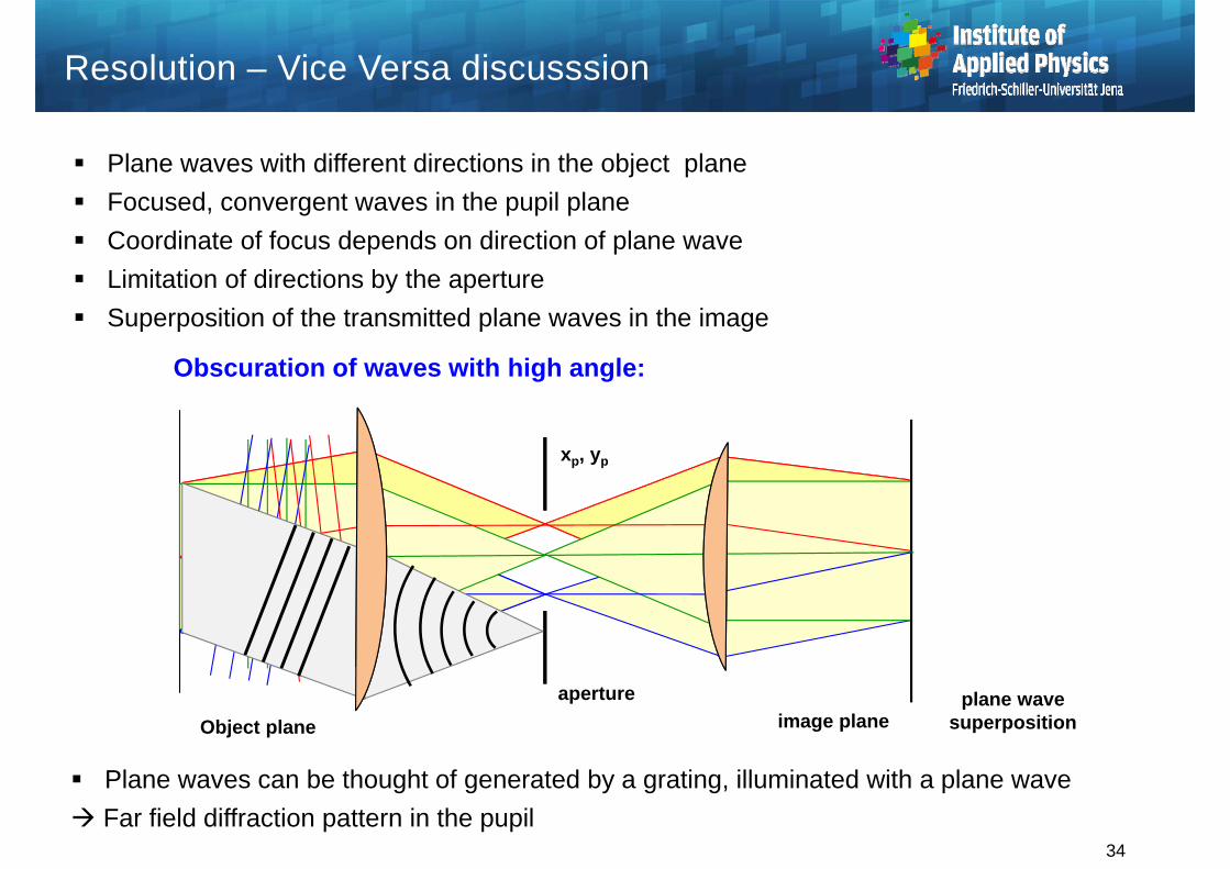
Plane waves with different directions in the object plane Focused, convergent waves in the pupil plane Coordinate of focus depends on direction of plane wave Limitation of directions by the aperture Superposition of the transmitted plane waves in the image
34
Object plane
apertureimage plane
xp, yp
plane wavesuperposition
Obscuration of waves with high angle:
Plane waves can be thought of generated by a grating, illuminated with a plane wave Far field diffraction pattern in the pupil
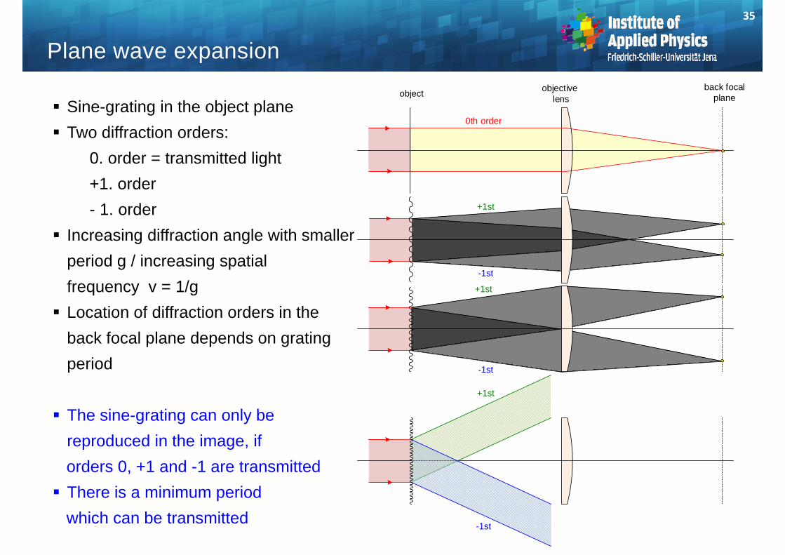
Sine-grating in the object plane Two diffraction orders:
0. order = transmitted light +1. order - 1. order
Increasing diffraction angle with smaller period g / increasing spatialfrequency v = 1/g Location of diffraction orders in the
back focal plane depends on grating period
The sine-grating can only be reproduced in the image, if orders 0, +1 and -1 are transmitted There is a minimum period
which can be transmitted
35
Plane wave expansion
+1st
-1st
+1st
-1st
+1st
-1st
objectback focal
planeobjective
lens
0th order
diffracted ray direction
objectstructure
g = 1 /
/ g
k
k x
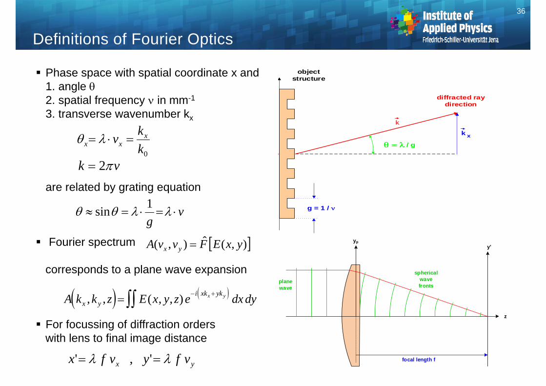
Definitions of Fourier Optics
Phase space with spatial coordinate x and1. angle 2. spatial frequency in mm-1
3. transverse wavenumber kx
are related by grating equation
Fourier spectrum
corresponds to a plane wave expansion
For focussing of diffraction orderswith lens to final image distance
0kkv x
xx
),(ˆ),( yxEFvvA yx
A k k z E x y z e dx dyx yi xk ykx y, , ( , , )
vk 2
vg
1sin
36
yx vfyvfx ',' focal length f
y'
planewave
spherical wave fronts
z
yp
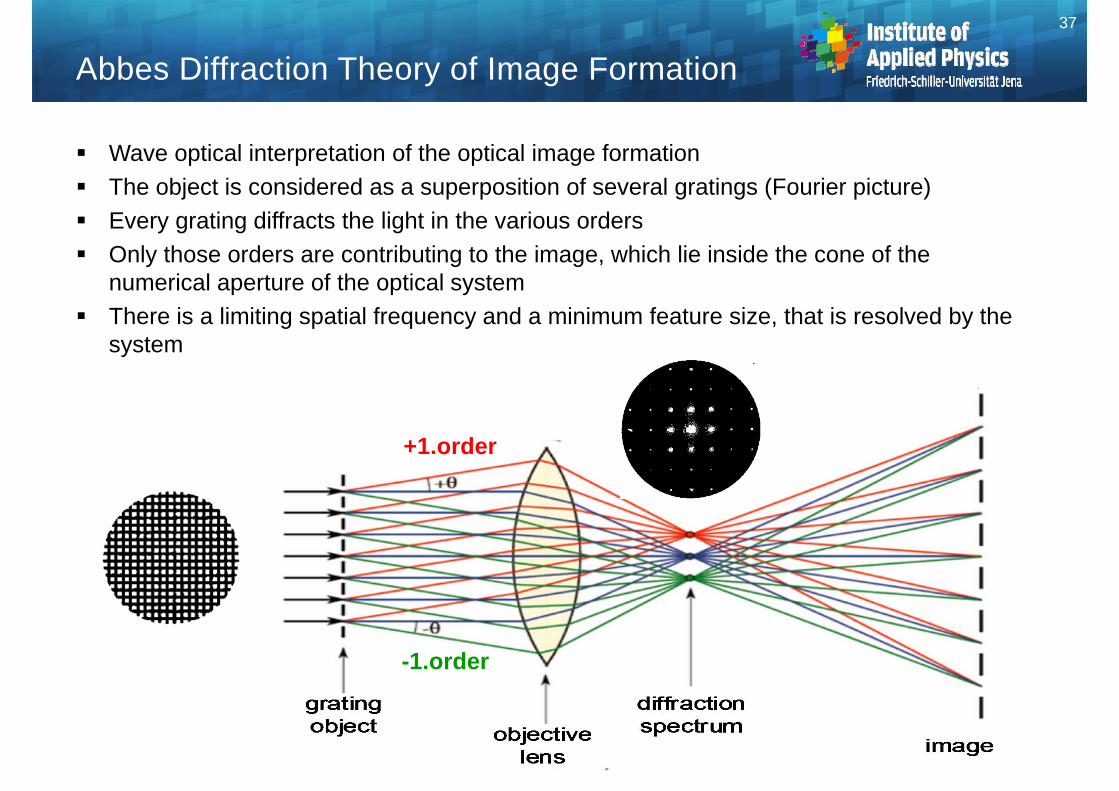
Abbes Diffraction Theory of Image Formation
Wave optical interpretation of the optical image formation The object is considered as a superposition of several gratings (Fourier picture) Every grating diffracts the light in the various orders Only those orders are contributing to the image, which lie inside the cone of the
numerical aperture of the optical system There is a limiting spatial frequency and a minimum feature size, that is resolved by the
system
+1.order
-1.order
37
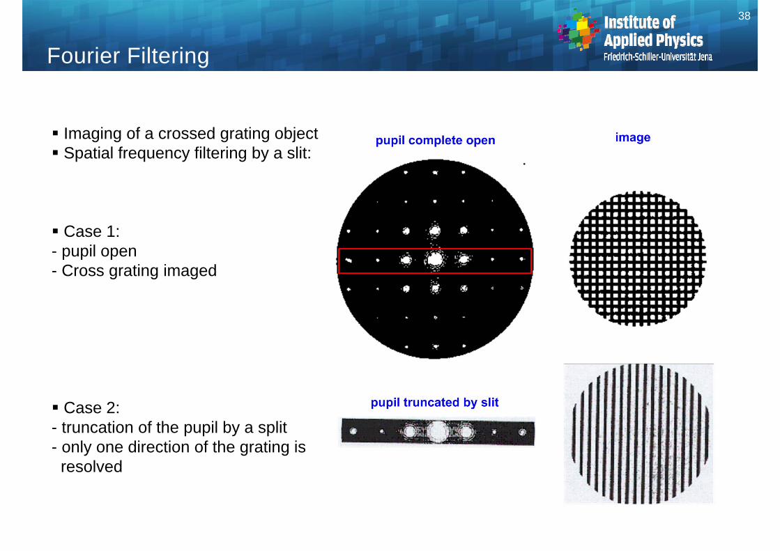
Imaging of a crossed grating object Spatial frequency filtering by a slit:
Case 1: - pupil open- Cross grating imaged
Case 2: - truncation of the pupil by a split- only one direction of the grating is
resolved
Fourier Filtering
38
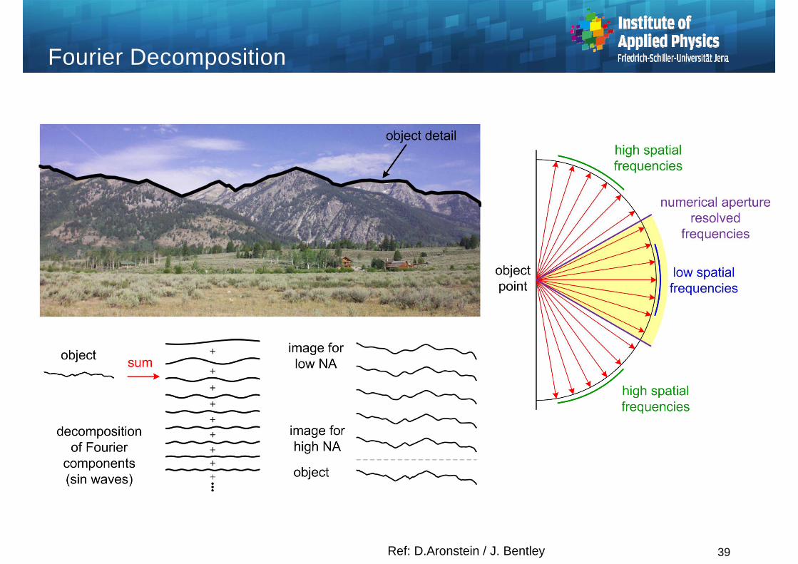
Fourier Decomposition
Ref: D.Aronstein / J. Bentley 39

40
-2 -1 0 1 20
0.5
1
-2 -1 0 1 2-1
0
1
-2 -1 0 1 2-0.5
0
0.5
-2 -1 0 1 2-1
0
1
-2 -1 0 1 2-0.5
0
0.5
-2 -1 0 1 2-1
0
1
-2 -1 0 1 2-0.5
0
0.5
-2 -1 0 1 2-1
0
1
-2 -1 0 1 2-0.5
0
0.5
-2 -1 0 1 2-1
0
1
Description of slit transmission as sumof cosine-functions
All object structures can be described as sum of cosine-functions
Cos_trafo.m
=
=
=
=
+
+
+
+
cos(x) where x = x/2
- sin(3x)/3
+ sin(5x)/5
- sin(7x)/7
+ sin(9x)/9
Fourier Components
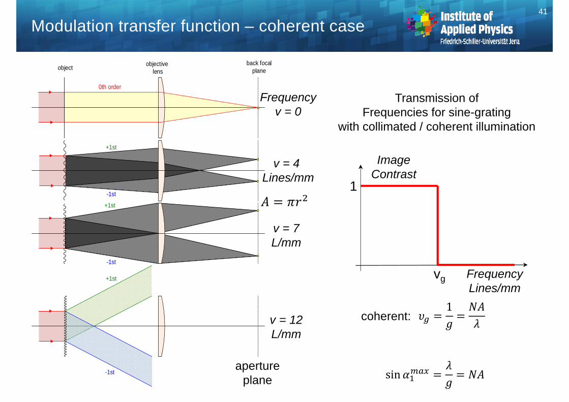
Modulation transfer function – coherent case41
Frequencyv = 0
Transmission of Frequencies for sine-grating
with collimated / coherent illumination
+1st
-1st
+1st
-1st
+1st
-1st
objectback focal
planeobjective
lens
0th order
v = 4 Lines/mm
v = 7L/mm
v = 12L/mm
FrequencyLines/mm
Image Contrast
1
coherent:
apertureplane sin
1
vg
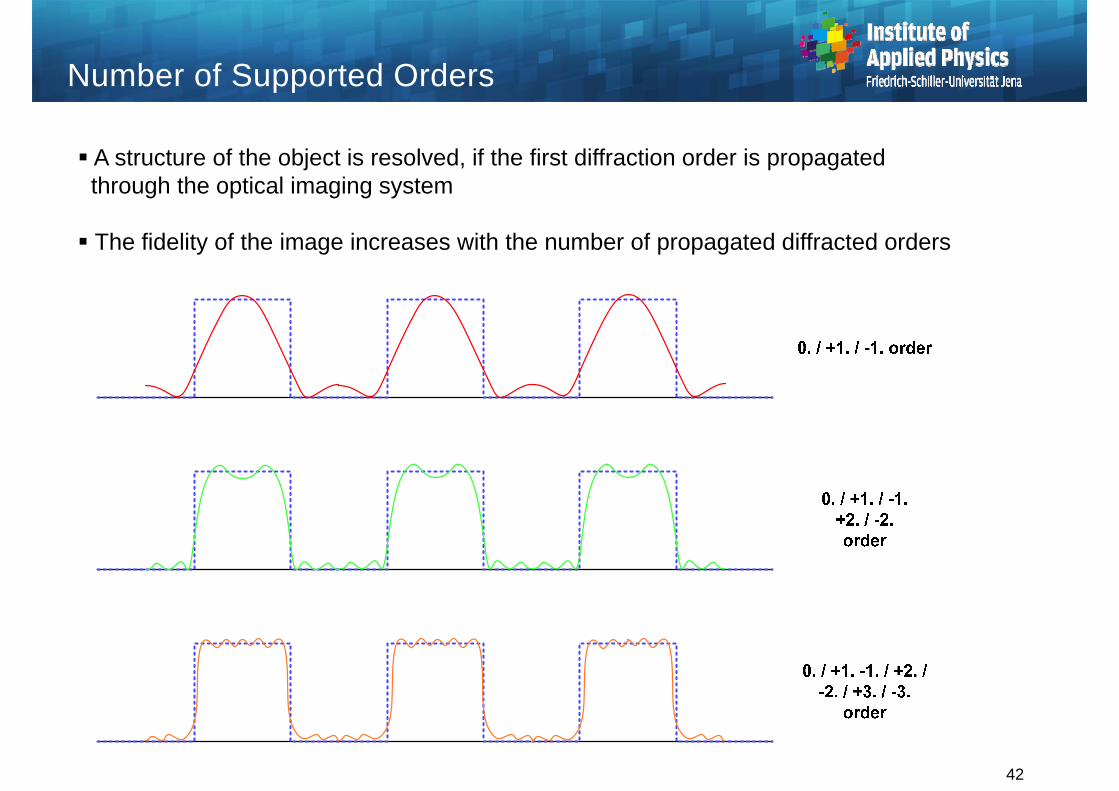
Number of Supported Orders
A structure of the object is resolved, if the first diffraction order is propagatedthrough the optical imaging system
The fidelity of the image increases with the number of propagated diffracted orders
42

Off-Axis illumination With an off-axis illumination the transmitted
and diffracted orders shift at the pupil The 2. order walks into the pupil, if Ill = NA With a set of illumination directions with
NAillumination = Naimaging e.g. approx. incoherent Incoherent cut off frequency
= two times the coherent cut off
NAg
2
Modulation transfer – off axis illumination
opticalsystem
object
diffracted ordersa) resolved
b) not resolved
+1.
+1.+2.
+2.
0.
-2.
-1.
0.
-2.
-1.
incidentlight
43
NAg
Coherent – collimated illumination
-1.
-1.
0.+2.+1.
0.
+1.
-2.
+2.+1.
NA
g NA
g
2
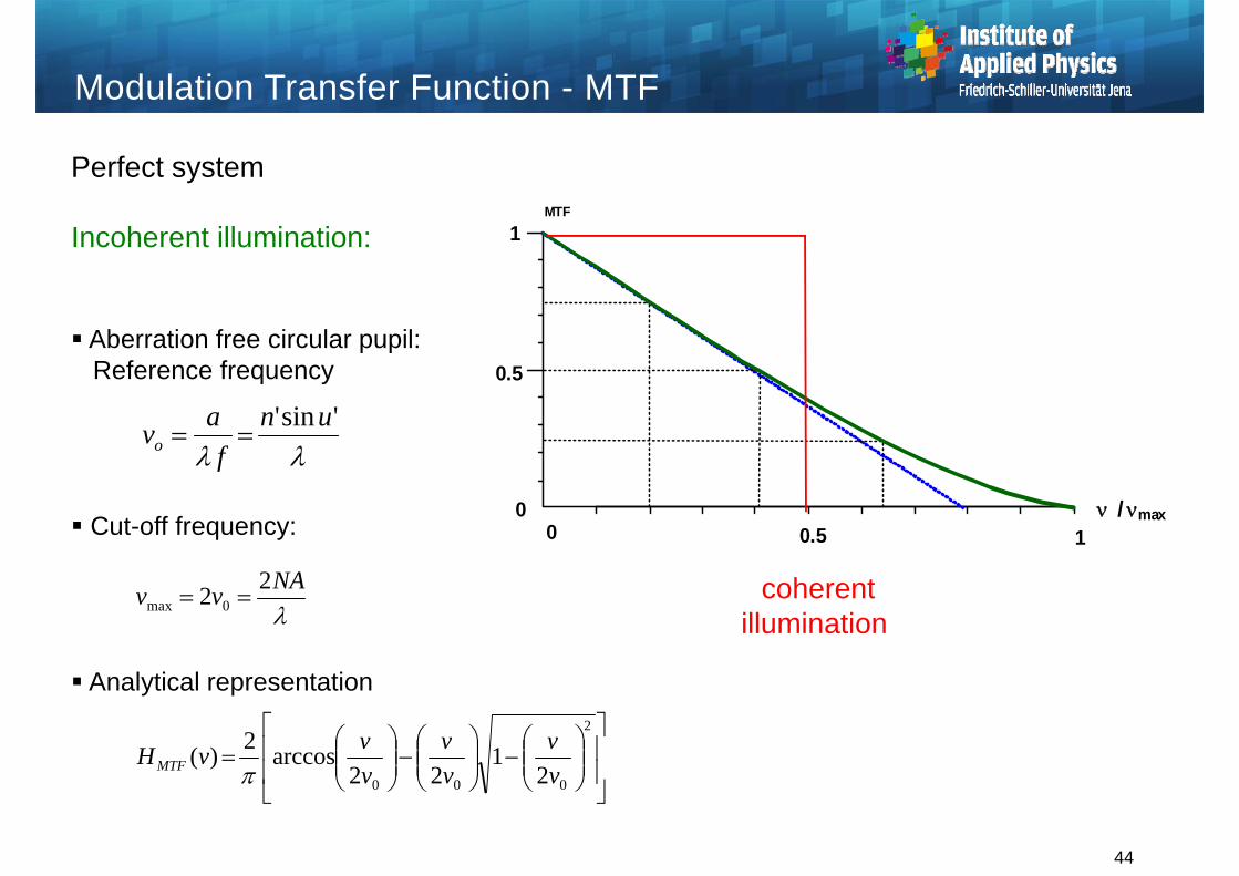
Modulation Transfer Function - MTF
Aberration free circular pupil:Reference frequency
Cut-off frequency:
Analytical representation
'sin' un
favo
NAvv 22 0max
2
000 21
22arccos2)(
vv
vv
vvvHMTF
/ max0
0
1
0.5 1
0.5
MTF
44
Perfect system
Incoherent illumination:
coherentillumination
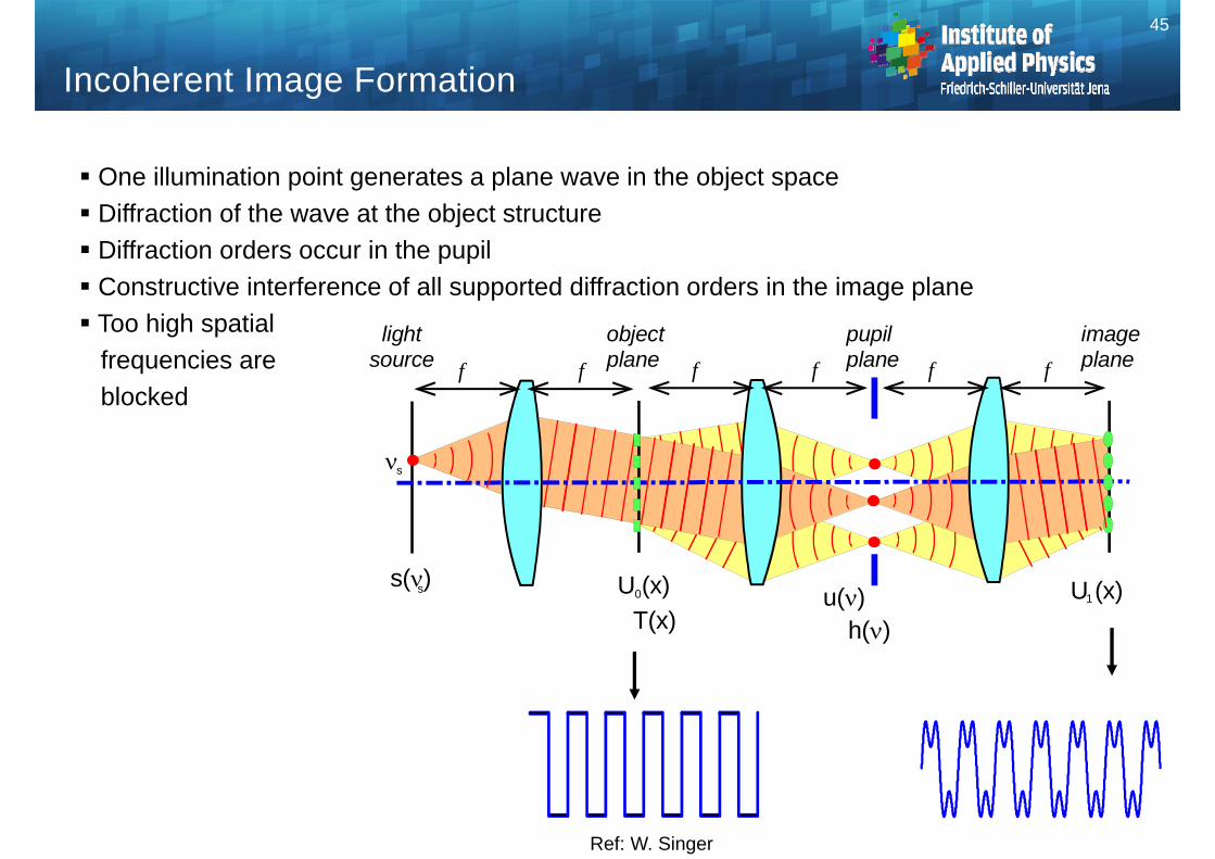
Incoherent Image Formation
One illumination point generates a plane wave in the object space Diffraction of the wave at the object structure Diffraction orders occur in the pupil Constructive interference of all supported diffraction orders in the image plane Too high spatial
frequencies areblocked
object plane
pupilplane
imageplanef f f f
u() U (x)1
h()
f f
lightsource
s() U (x)0
T(x)
s
s
Ref: W. Singer
45
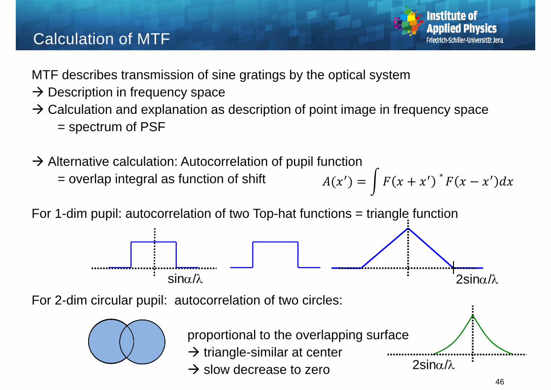
Calculation of MTF
46
MTF describes transmission of sine gratings by the optical system Description in frequency space Calculation and explanation as description of point image in frequency space
= spectrum of PSF
Alternative calculation: Autocorrelation of pupil function = overlap integral as function of shift
For 1-dim pupil: autocorrelation of two Top-hat functions = triangle function
For 2-dim circular pupil: autocorrelation of two circles:
proportional to the overlapping surface triangle-similar at center slow decrease to zero
2sin/sin/
2sin/
∗
pp
vyvxipppsfyxOTF dydxeyxINvvH ypxp
2),(),(
),(ˆ),( yxIFvvH PSFyxOTF
p
xp
xpxOTF dxvfxPvfxPvH
22)( *
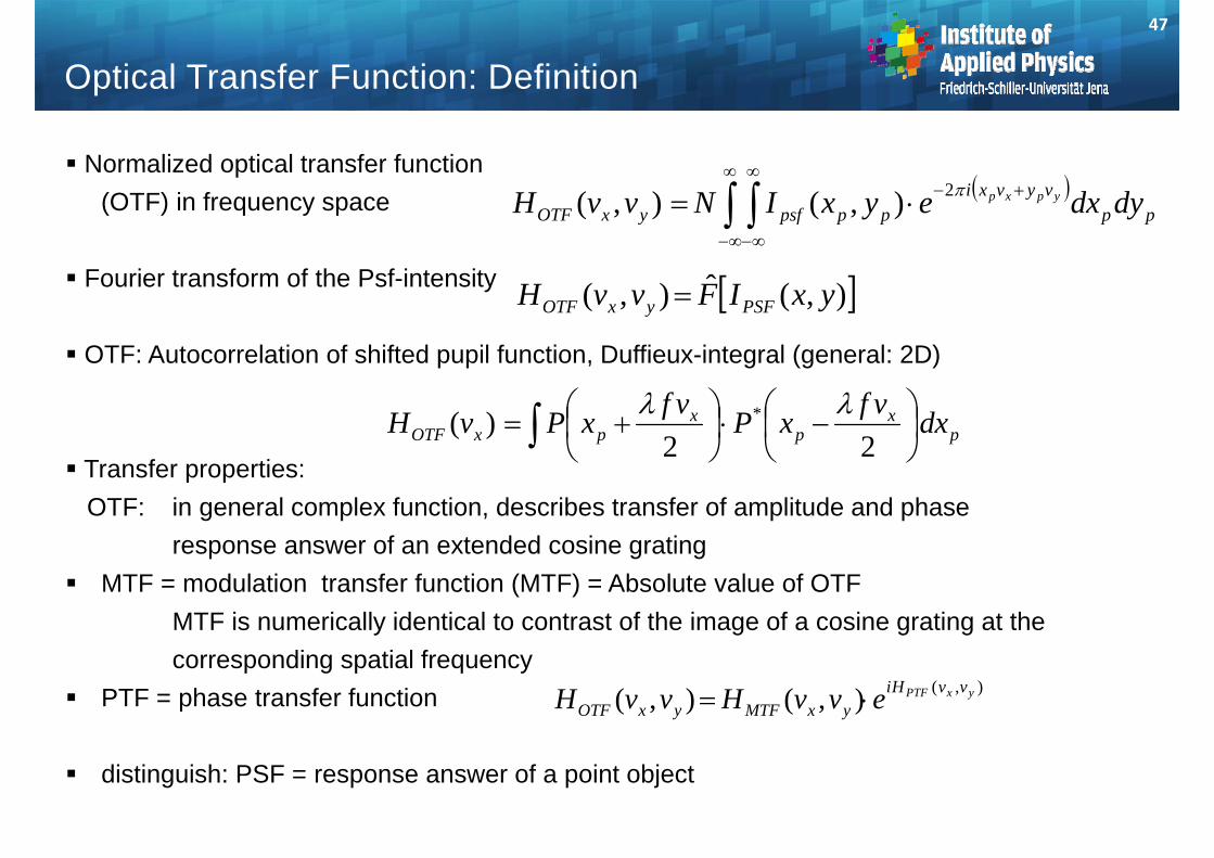
Optical Transfer Function: Definition
Normalized optical transfer function(OTF) in frequency space
Fourier transform of the Psf-intensity
OTF: Autocorrelation of shifted pupil function, Duffieux-integral (general: 2D)
Transfer properties:OTF: in general complex function, describes transfer of amplitude and phase
response answer of an extended cosine grating MTF = modulation transfer function (MTF) = Absolute value of OTF
MTF is numerically identical to contrast of the image of a cosine grating at thecorresponding spatial frequency
PTF = phase transfer function
distinguish: PSF = response answer of a point object
47
),(),(),( yxPTF vvHiyxMTFyxOTF evvHvvH

MTF of a Perfect System Loss of contrast for higher spatial frequencies
48
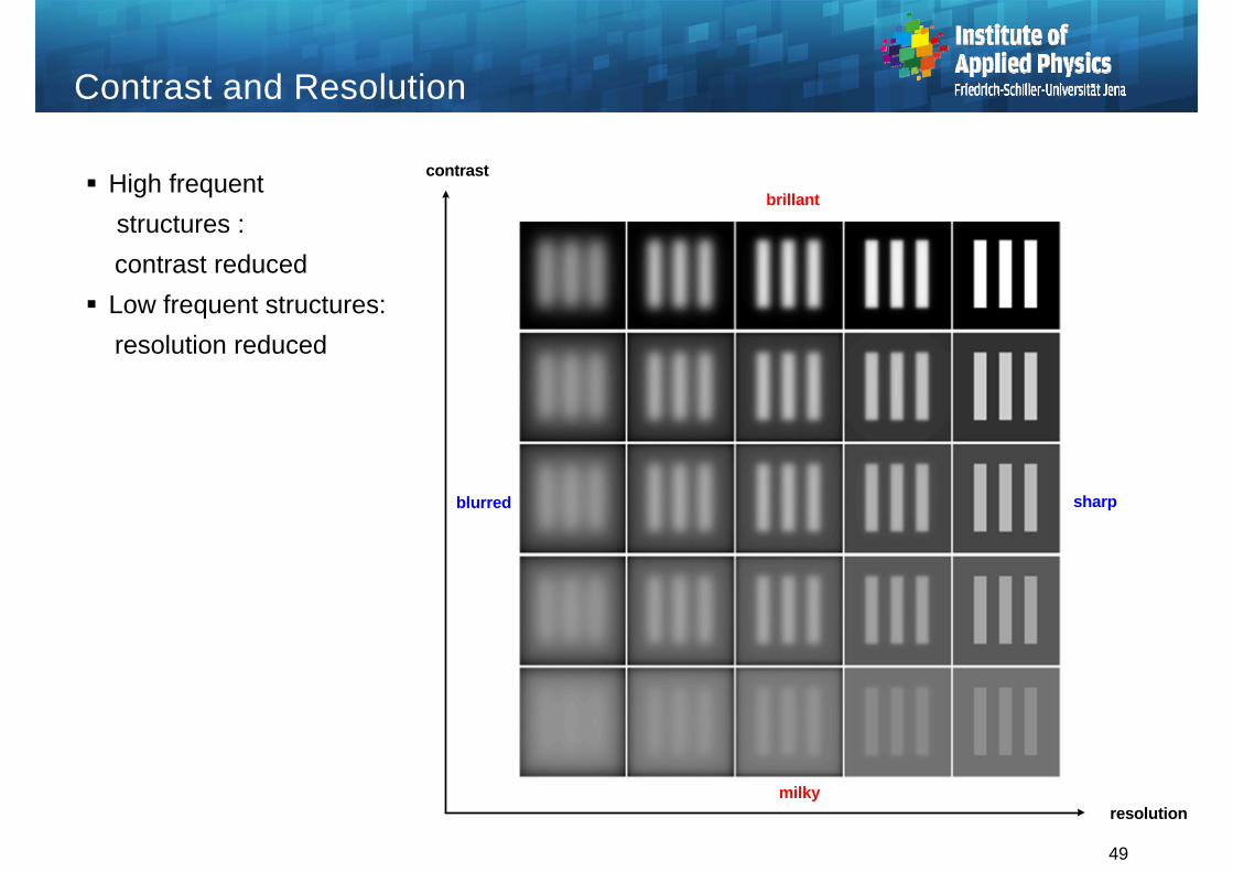
Contrast and Resolution
High frequent structures :contrast reduced
Low frequent structures:resolution reduced
contrast
resolution
brillant
sharpblurred
milky
49
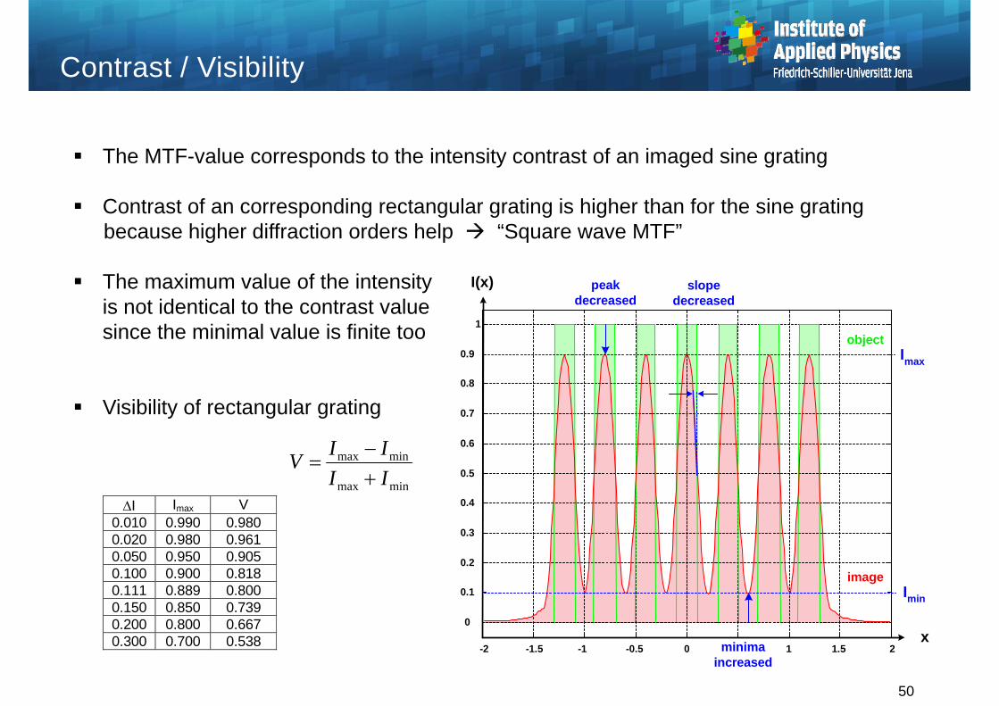
I Imax V 0.010 0.990 0.980 0.020 0.980 0.961 0.050 0.950 0.905 0.100 0.900 0.818 0.111 0.889 0.800 0.150 0.850 0.739 0.200 0.800 0.667 0.300 0.700 0.538
Contrast / Visibility
The MTF-value corresponds to the intensity contrast of an imaged sine grating
Contrast of an corresponding rectangular grating is higher than for the sine gratingbecause higher diffraction orders help “Square wave MTF”
The maximum value of the intensityis not identical to the contrast valuesince the minimal value is finite too
Visibility of rectangular grating
minmax
minmax
IIIIV
I(x)
-2 -1.5 -1 -0.5 0 1 1.5 2
0
0.1
0.2
0.3
0.4
0.5
0.6
0.7
0.8
0.9
1
x
Imax
Imin
object
image
peakdecreased
slopedecreased
minimaincreased
50
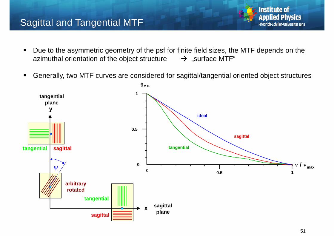
Due to the asymmetric geometry of the psf for finite field sizes, the MTF depends on theazimuthal orientation of the object structure „surface MTF“
Generally, two MTF curves are considered for sagittal/tangential oriented object structures
Sagittal and Tangential MTF
y
tangentialplane
tangential sagittal
arbitraryrotated
x sagittalplane
tangential
sagittal
gMTF
tangential
ideal
sagittal
1
0
0.5
0 0.5 1 / max
51

Polychromatic MTF
Cut off frequency depends on
Polychromatic MTF: Spectral incoherent weighted superposition of monochromatic MTF’s
Example: uncorrected axial color F (486), D(587), C(656nm) with SF6 instead SF5
0
)( ),()()( dvHSvH MTFpoly
MTF
52
#122 0max F
NAvv
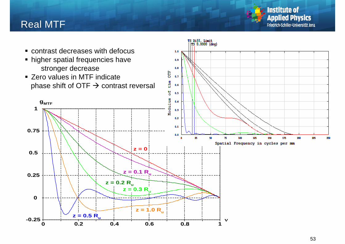
contrast decreases with defocus higher spatial frequencies have
stronger decrease Zero values in MTF indicate
phase shift of OTF contrast reversal
Real MTF
z = 0
z = 0.1 Ru
gMTF1
0.75
0.25
0.5
0
-0.250 0.2 0.4 0.6 0.8 1
z = 0.2 Ruz = 0.3 Ru
z = 1.0 Ruz = 0.5 Ru
53
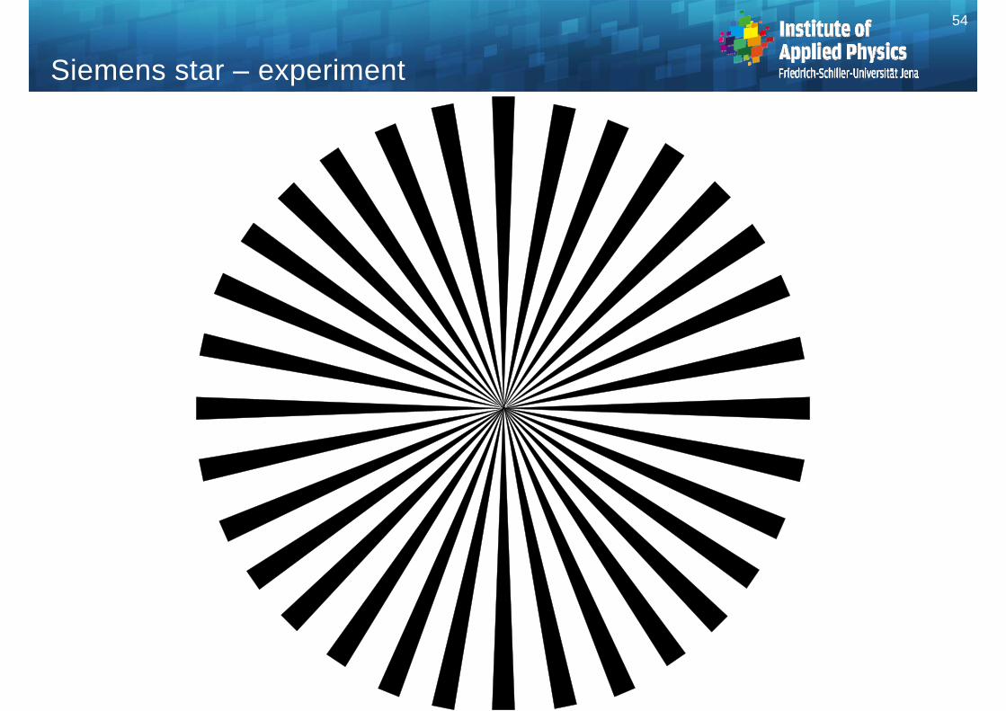
Siemens star – experiment
54

Test: Siemens Star
Determination of resolution and contrast with Siemens star test chart:
Central segments b/w Growing spatial frequency towards the
center Gray ring zones: contrast zero Calibrating spatial feature size by radial
diameter Nested gray rings with finite contrast
in between:contrast reversal pseudo resolutionPhase shift in transfer function
55
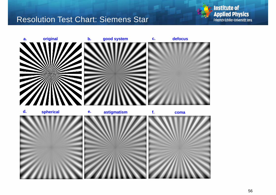
Resolution Test Chart: Siemens Star
original good system
astigmatism comaspherical
defocusa. b. c.
d. e. f.
56
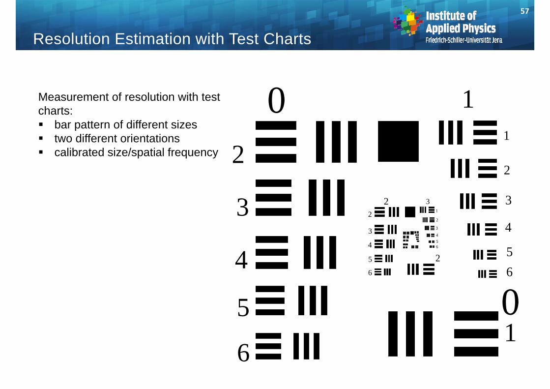
Resolution Estimation with Test Charts
0 1
10
2
3
4
5
6
65
4
3
2
1
6
5
4
3
22 3
1
2
3
2
456
Measurement of resolution with test charts: bar pattern of different sizes two different orientations calibrated size/spatial frequency
57

Contrast / Resolution of Real Images
Degradation due to1. loss of contrast2. loss of resolution
58

Contrast as a function of spatial frequency
Compromise betweenresolution and visibiltyis not trivial and dependson application
Contrast and Resolution of Real Applications
59
Real systems:
Limited contrast sensitivity of detectors
for instance: 8Bit = 256ct limit 1/256 for contrast
contrast sensitivity may depend on direction and spatial frequency
Image processing with contrast enhancement
Human eye: about 0,25% contrast sensitivity v/vreal
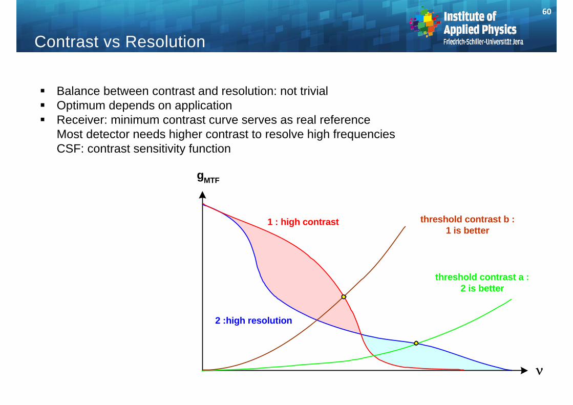
Balance between contrast and resolution: not trivial Optimum depends on application Receiver: minimum contrast curve serves as real reference
Most detector needs higher contrast to resolve high frequenciesCSF: contrast sensitivity function
Contrast vs Resolution
gMTF
1 : high contrast
2 :high resolution
threshold contrast a :2 is better
threshold contrast b :1 is better
60
Fourier theory of image formation
Coherent and incoherent image formation
61
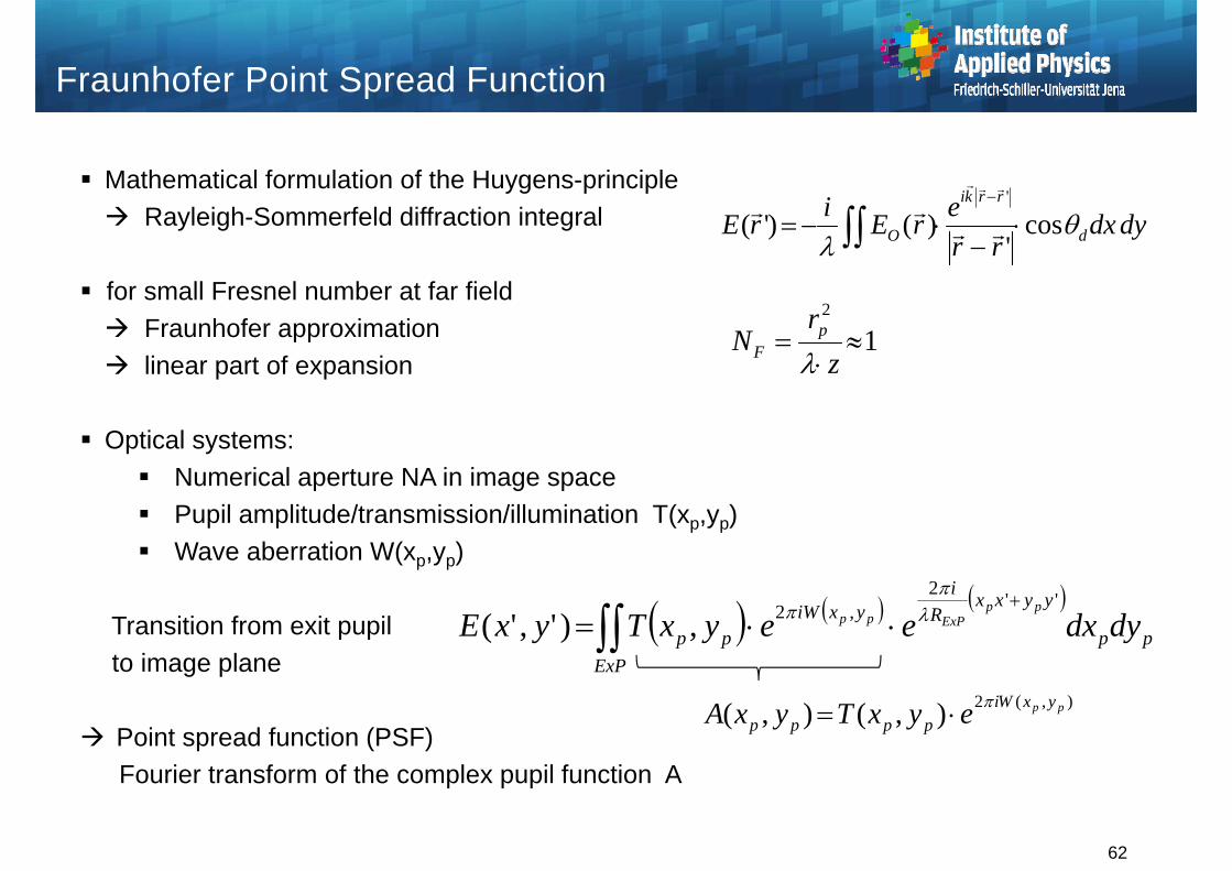
Fraunhofer Point Spread Function
Mathematical formulation of the Huygens-principle Rayleigh-Sommerfeld diffraction integral
for small Fresnel number at far field Fraunhofer approximation linear part of expansion
Optical systems: Numerical aperture NA in image space Pupil amplitude/transmission/illumination T(xp,yp) Wave aberration W(xp,yp)
Transition from exit pupilto image plane
Point spread function (PSF) Fourier transform of the complex pupil function A
12
z
rN p
F
),(2),(),( pp yxWipppp eyxTyxA
pp
yyxxR
iyxiW
ppExP
dydxeeyxTyxEpp
ExPpp''2
,2,)','(
dydxrr
erEirE d
rrki
O
cos'
)()'('
62
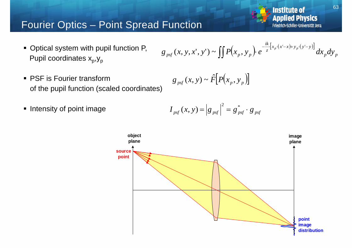
Fourier Optics – Point Spread Function
Optical system with pupil function P,Pupil coordinates xp,yp
PSF is Fourier transformof the pupil function (scaled coordinates)
Intensity of point image
pp
yyyxxxzik
pppsf dydxeyxPyxyxg pp '',~)',',,(
pppsf yxPFyxg ,ˆ~),(
objectplane
imageplane
sourcepoint
pointimagedistribution
63
psfpsfpsfpsf gggyxI *2),(
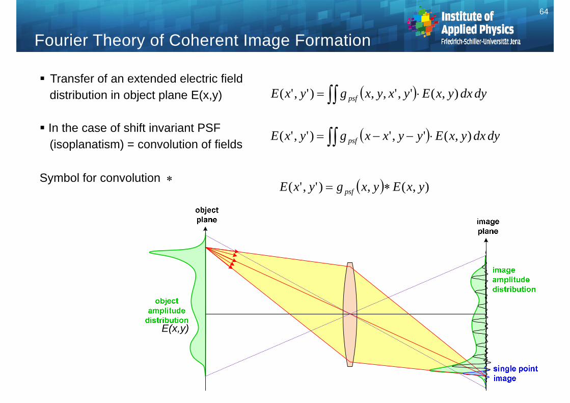
Fourier Theory of Coherent Image Formation
Transfer of an extended electric fielddistribution in object plane E(x,y)
In the case of shift invariant PSF (isoplanatism) = convolution of fields
Symbol for convolution
dydxyxEyxyxgyxE psf ),(',',,)','(
dydxyxEyyxxgyxE psf ),(',')','(
64
E(x,y)
),(,)','( yxEyxgyxE psf
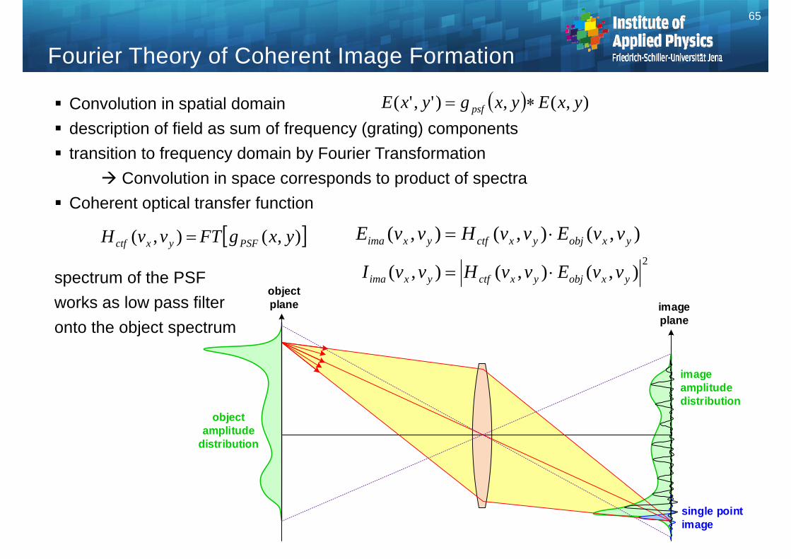
Fourier Theory of Coherent Image Formation
Convolution in spatial domain description of field as sum of frequency (grating) components transition to frequency domain by Fourier Transformation
Convolution in space corresponds to product of spectra Coherent optical transfer function
spectrum of the PSF works as low pass filter onto the object spectrum
),(),( yxgFTvvH PSFyxctf ),(),(),( yxobjyxctfyxima vvEvvHvvE 2
),(),(),( yxobjyxctfyxima vvEvvHvvI
65
objectplane image
plane
objectamplitude
distribution
single pointimage
imageamplitudedistribution
),(,)','( yxEyxgyxE psf
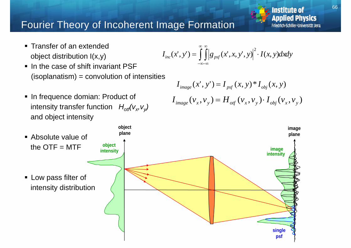
Fourier Theory of Incoherent Image Formation
objectintensity image
intensity
singlepsf
objectplane
imageplane
Transfer of an extendedobject distribution I(x,y) In the case of shift invariant PSF
(isoplanatism) = convolution of intensities
In frequence domian: Product ofintensity transfer function Hotf(vx,vy)and object intensity
Absolute value ofthe OTF = MTF
Low pass filter ofintensity distribution
),(*),()','( yxIyxIyxI objpsfimage
dydxyxIyyxxgyxI psfinc
),(),',,'()','(2
66
),(),(),( yxobjyxotfyximage vvIvvHvvI
Modulation Transfer
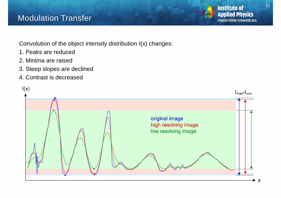
Convolution of the object intensity distribution I(x) changes:1. Peaks are reduced2. Minima are raised3. Steep slopes are declined4. Contrast is decreased
67
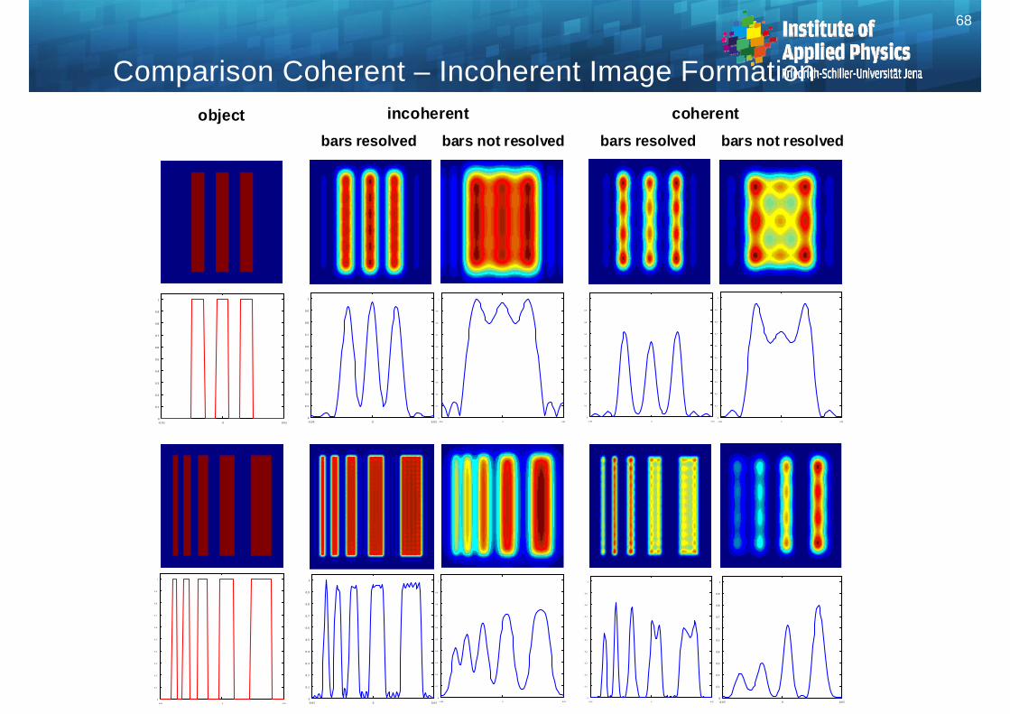
Comparison Coherent – Incoherent Image Formationobject
‐0.05 0 0.05
0
0.1
0.2
0.3
0.4
0.5
0.6
0.7
0.8
0.9
1
incoherent coherent
‐0.0 5 0 0.0 50
0.1
0.2
0.3
0.4
0.5
0.6
0.7
0.8
0.9
1
‐0.05 0 0.05
0
0.1
0.2
0.3
0.4
0.5
0.6
0.7
0.8
0.9
1
‐0.05 0 0.05
0
0.1
0.2
0.3
0.4
0.5
0.6
0.7
0.8
0.9
1
‐0.0 5 0 0.0 50
0.1
0.2
0.3
0.4
0.5
0.6
0.7
0.8
0.9
1
‐0.0 5 0 0.0 50
0.1
0.2
0.3
0.4
0.5
0.6
0.7
0.8
0.9
1
‐0.0 5 0 0.0 50
0.1
0.2
0.3
0.4
0.5
0.6
0.7
0.8
0.9
1
‐0.05 0 0.05
0
0.1
0.2
0.3
0.4
0.5
0.6
0.7
0.8
0.9
1
‐0.05 0 0.05
0
0.1
0.2
0.3
0.4
0.5
0.6
0.7
0.8
0.9
1
‐0.05 0 0.05
0
0.1
0.2
0.3
0.4
0.5
0.6
0.7
0.8
0.9
1
bars resolved bars not resolved bars resolved bars not resolved
68
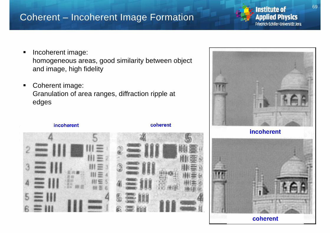
Incoherent image: homogeneous areas, good similarity between objectand image, high fidelity
Coherent image:Granulation of area ranges, diffraction ripple atedges
Coherent – Incoherent Image Formation69
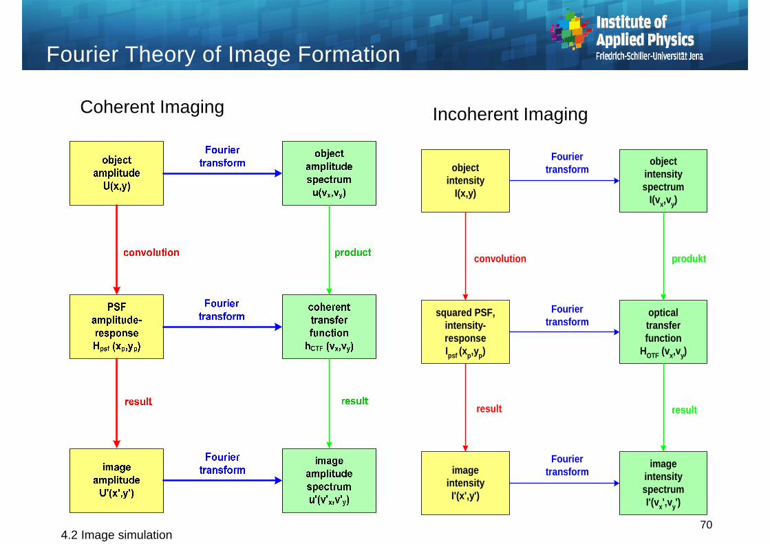
Fourier Theory of Image Formation
Coherent Imaging
objectintensity
I(x,y)
squared PSF,intensity-responseIpsf (xp,yp)
imageintensityI'(x',y')
convolution
result
objectintensityspectrum
I(vx,vy)
opticaltransferfunction
HOTF (vx,vy)
imageintensityspectrumI'(vx',vy')
produkt
result
Fouriertransform
Fouriertransform
Fouriertransform
Incoherent Imaging
4.2 Image simulation70

Partial Coherent Imaging
Every object point is illuminated by an angle spectrum due to the finite extend of the source In the pupil the diffraction orders are broadened no full constructive interference in the image plane
source condenser object lens image
angle shift
71
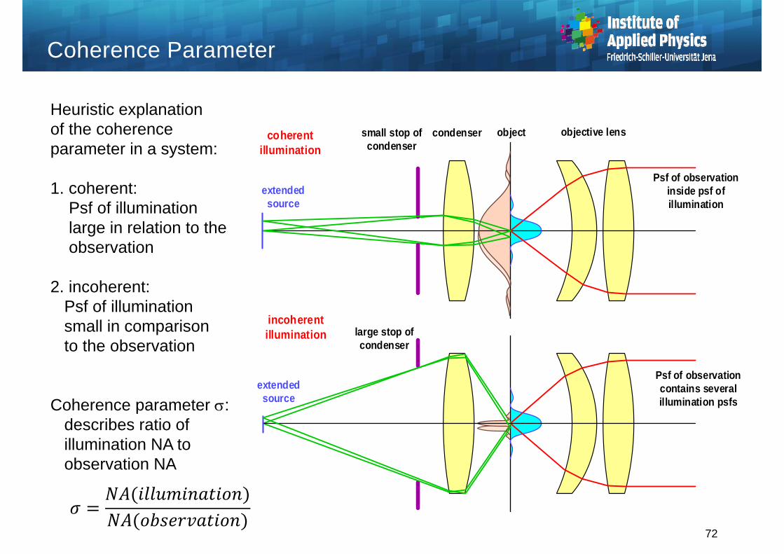
Heuristic explanationof the coherenceparameter in a system:
1. coherent:Psf of illuminationlarge in relation to theobservation
2. incoherent:Psf of illuminationsmall in comparison to the observation
Coherence parameter : describes ratio of illumination NA to observation NA
object objective lenscondensersmall stop of condenser
extended source
coherentillumination
large stop of condenser
incoherentillumination
Psf of observation inside psf of illumination
Psf of observation contains several illumination psfs
extended source
Coherence Parameter
72
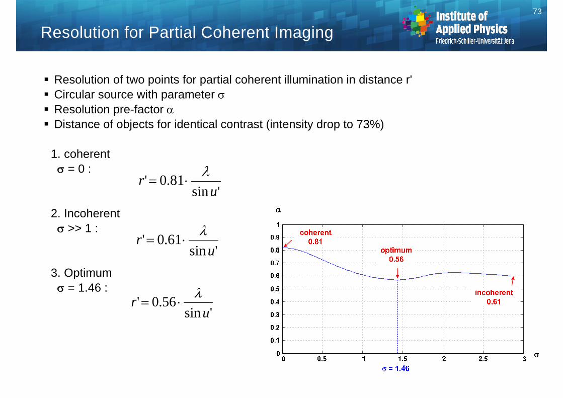
Resolution of two points for partial coherent illumination in distance r' Circular source with parameter Resolution pre-factor Distance of objects for identical contrast (intensity drop to 73%)
1. coherent = 0 :
2. Incoherent >> 1 :
3. Optimum = 1.46 :
Resolution for Partial Coherent Imaging
'sin81.0'
ur
'sin61.0'
ur
'sin56.0'
ur
73

Resolution and Contrast for Partial Coherent Imaging
Transfer of spatial frequenciesdepend on illumination settingsand directions
Analytical representationonly for circular Symmetrypossible (Kintner)
Transfer capability dependson integration overlap ofillumination and detectionpupils
incoherentpartial
coherent coherentpartial coherent
oblique illuminationcoherent oblique
illumination
74
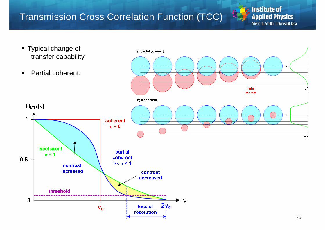
Transmission Cross Correlation Function (TCC)
Typical change oftransfer capability
Partial coherent:
75
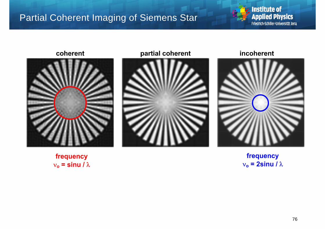
Partial Coherent Imaging of Siemens Star
76

Pupil Illumination Pattern
Coherent
Off Axis Annular Annular
Dipole Rotated Dipole
Disk = 0.5 Disk = 0.8
6 -Channel
Variation of the pupil illumination Enhancement of resolution Improvement of contrast Object specific optimization
Often the best compromise with partial coherent illumination where slightly increased intensity at the
edges
In microscopy the adjustment of Koehler illumination corresponds to choosing this setup
Ref: W. Singer
77
Dark field illumination in microscopy
Foucault knife edge method for aberration measurement
Schlieren method for measurement of striae and inhomogeneities in materials
Zernike contrast method in microscopy
Use of apodization for suppression of diffraction rings, resolution enhancing masks
Beam clean up of laser radiation with kepler system and mode stop
Edge enhancement techniques in lithography
Oblique illumination for resolution enhancement in microscopy
Schmidt corrector plate in astronomical telescopes
Pupil filter masks to generate extended depth of focus
Resolution enhancement by structured illumination
Applications of Fourier Filtering Techniques
78