Exact cancellation of emittance growth due to coupledtransverse dynamics in solenoids and rf couplers

David H. Dowell,* Feng Zhou, and John SchmergeSLAC National Accelerator Laboratory, 2575 Sand Hill Road, Menlo Park, California 94025, USA

(Received 25 July 2017; published 17 January 2018)

Weak, rotated magnetic and radio frequency quadrupole fields in electron guns and injectors can couplethe beam’s horizontal with vertical motion, introduce correlations between otherwise orthogonal transversemomenta, and reduce the beam brightness. This paper discusses two important sources of coupledtransverse dynamics common to most electron injectors. The first is quadrupole focusing followed by beamrotation in a solenoid, and the second coupling comes from a skewed high-power rf coupler or cavity portwhich has a rotated rf quadrupole field. It is shown that a dc quadrupole field can correct for both types ofcouplings and exactly cancel their emittance growths. The degree of cancellation of the rf skew quadrupoleemittance is limited by the electron bunch length. Analytic expressions are derived and compared withemittance simulations and measurements.

DOI: 10.1103/PhysRevAccelBeams.21.010101

I. INTRODUCTION

Optical aberrations are a major limitation to the beamquality of modern electron injectors and accelerators. Thisis especially true for the low-voltage guns and injectorsrequired for high-duty factor and high-average currentoperation. In these systems, the beam is made large tomitigate space-charge forces. However, this large beam ismore sensitive to aberrations such as the spherical aberra-tion, which increases the emittance as the fourth power ofthe transverse beam size, and the chromatic aberration,which is proportional to the beam size squared.Here we examine the coupled transverse dynamics

aberration, which also strongly depends on the beam size.Coupled transverse dynamics results when the electronshave azimuthal momenta and their trajectories are no longercoplanar with the beam axis. The trajectories are ”coupled”because the electron’s x coordinate depends not just on xand x0 but also on y and y0, and similarly for the ycoordinate. This paper assumes the mathematical theoryis linear and applies 4 × 4-matrix algebra to compute theelectron dynamics. We concentrate on the 4D transforma-tion of a rotated quadrupole which skews the electronsabout the beam axis. Since the 4D rotation is linear, the 4Demittance does not grow. However, there is emittancegrowth in both the x-x0 and y-y0 2D phase spaces due to

skew trajectories. Fortunately, the theory and simulationshow that it can be eliminated with a rotated corrector field,because the coupling is correlated.In his 1970 Ph.D. thesis, Ripken described a theory of

the coupled transverse dynamics in electron storage ringsfor high-energy physics experiments [1]. His and studieswhich followed [2] used 4D-matrix algebra to show that thebeam luminosity could be increased (emittance decreased)by correcting for transverse plane coupling with a skewquadrupole. Recent theoretical work describes the coupleddynamics by generalizing the Courant-Snyder theory witha 4D symplectic rotation [3]. A useful introduction tothe matrix theory for electron beams can be found inWiedemann’s book [4].This paper concentrates on beam quality degradation due

to quadrupole fields which are themselves rotated or whenthe beam has been rotated in a solenoid with respect tonormally aligned quadrupole fields. Herewe study two beamline components which are common sources of rotatedquadrupole fields. The first is a weak quadrupole fieldfollowed by a solenoid, and the second is the quadrupolefield produced by the coupler which feeds rf power into acavity through rotated or unbalanced ports [5,6].The emittance of quadrupole followed by a solenoid is

simply the emittance growth of the rotated quadrupolefield, with a rotation angle equal to the sum of thequadrupole’s rotation plus the beam’s Larmor rotation inthe solenoid. Although we assume the weak quadrupolefield is near the solenoid, the field can, in fact, be anywherebefore the solenoid. This includes the quadrupole rf fieldsof a rf gun followed by a focusing solenoid.The transverse coupling due to rf fields can be eliminated

by canceling the on-axis dipole and quadrupole fields with

*dowell@slac.stanford.edu

Published by the American Physical Society under the terms ofthe Creative Commons Attribution 4.0 International license.Further distribution of this work must maintain attribution tothe author(s) and the published article’s title, journal citation,and DOI.

PHYSICAL REVIEW ACCELERATORS AND BEAMS 21, 010101 (2018)

2469-9888=18=21(1)=010101(14) 010101-1 Published by the American Physical Society

a dual rf feed and a racetracklike cavity shape [7]. Suchdesigns have been implemented into modern rf guns [8] andupgraded rf couplers for room temperature linacs [9].However, many accelerator rf cavities are built withoutthese features, because the designs already exist, and theredesign, fabrication, and testing costs of new rf structuresare prohibitively expensive, especially for superconductingrf cavities. Fortunately, as will be shown in this paper, muchof this rework is unnecessary, since the quadrupole rf fieldcan be exactly canceled with a low-field dc quadrupole.This paper is organized as follows. The next section

defines the terms rotated, normal, and skew quadrupolefields and derives the emittance growth produced by arotated quadrupole field. Section III gives a general dis-cussion of the fields of ideal solenoids, with only radialfields, and realistic solenoids possessing quadrupole fields.Quadrupole field measurements for a solenoid are pre-sented. In Sec. IV, expressions for the coupled transversedynamics emittance of the beam in a solenoid preceded bya weak quadrupole field are derived, and the emittancecancellation with a corrector quadrupole is demonstratedusing analytic and numerical calculations as well asmeasurements. Section V discusses the rf quadrupole field,its induced emittance growth, and emittance cancellationwith a dc corrector quadrupole. Finally, a summary of thework is presented in Sec. VI.

II. EMITTANCE GROWTH DUE TO ROTATED,NORMAL, AND SKEW QUADRUPOLE FIELDS

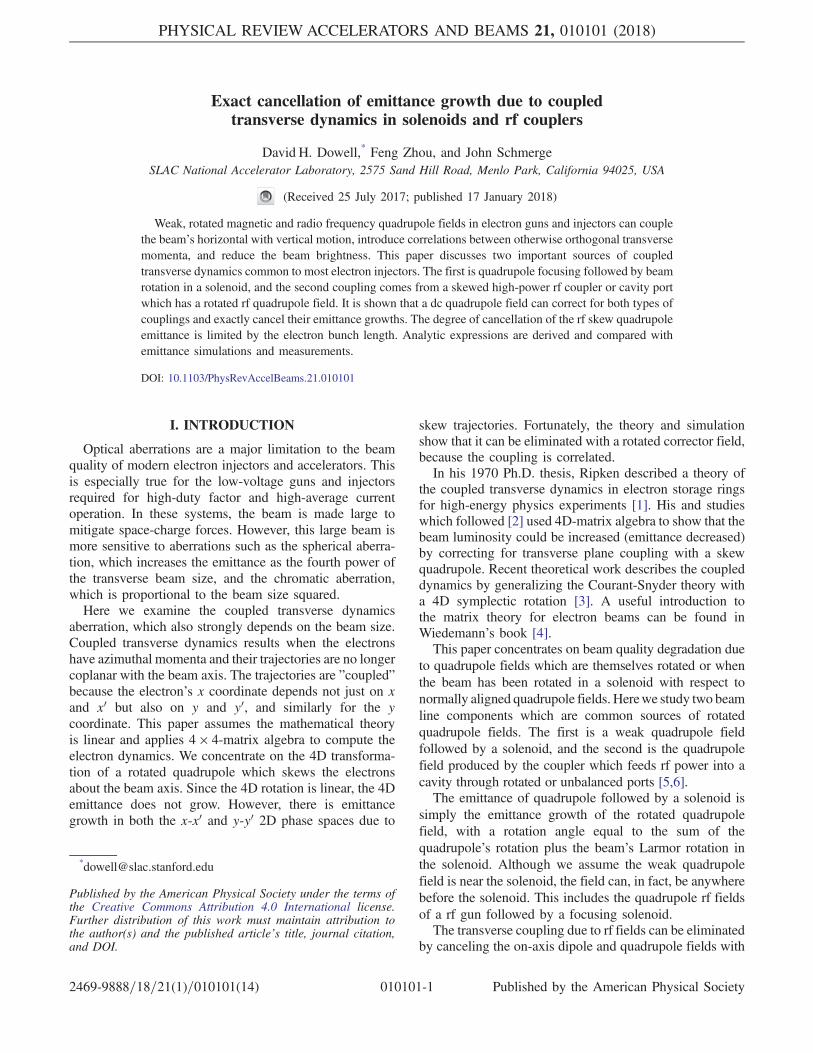
Figure 1 shows the equipotential surfaces for quadrupolemagnetic fields with rotated, normal, and skew Bθ-fieldpatterns. The normal-quadrupole field (center drawing inFig. 1) is aligned to the midplane of symmetry withByðx; yÞ ¼ −Byðx;−yÞ and Bxðx; y ¼ 0Þ ¼ 0 along the xaxis. Rotating the field 45° about the þz axis (out of thepage) results in a skew quadrupole field (right drawing inFig. 1). The term rotated quadrupole is given to a quadru-pole field having an arbitrary angle of axial rotation withrespect to the normal-quadrupole field orientation. The

rotated quadrupole field is equal to the vector sum ofnormal and skew quadrupole fields. As will be shown, onlythe skew component of a rotated quadrupole generatesemittance, and therefore only a skew quadrupole correctoris necessary to cancel the emittance growth. The normalcomponent of a rotated quadrupole produces no emittance;however, including a normal-quadrupole corrector allowsreturning the beam to its original transverse shape.The beam transformation matrix for a quadrupole rotated

about the þz axis is found by first rotating the beam aboutthe z axis, then transforming through a normal quadrupole,and lastly rotating the beam back to zero rotation. Using thematrix and angle conventions of the TRANSPORT and MAD

optics codes [10], the transformation matrix for a rotatedquadrupole is given by

Rrotquadðα; fÞ ¼ Rrotð−αÞRquadðfÞRrotðαÞ: ð1ÞHere Rrot and Rquad are the standard 4 × 4matrices which

rotate and quadrupole-focus the beam, respectively. Rrotrotates the beam clockwise an angle α about the positive zaxis. Therefore, the quadrupole rotation angle α is showngoing counterclockwise in Fig. 1. Rquad is for a thinquadrupole lens with focal length f. Multiplying thematrices gives the transformation matrix for a thin quadru-pole lens with focal length f and rotation angle α as

Rrotquadðα; fÞ ¼

0BBBBB@

1 0 0 0

− cos 2αf 1 − sin 2α

f 0

0 0 1 0− sin 2α

f 0 cos 2αf 1

1CCCCCA: ð2Þ

The focal strength depends upon the beam energy andthe integrated quadrupole field gradient:

1

f¼ e

βγmcLeff

∂By

∂x����x;y¼0

: ð3Þ

FIG. 1. Magnetic equipotential surfaces for rotated, normal, and skew quadrupole fields. The coordinate system is right-handed withthe z axis pointing out of the page. The normal-quadrupole field is focusing in the x plane and defocusing in the y plane for electronstraveling along the þz axis.

DOWELL, ZHOU, and SCHMERGE PHYS. REV. ACCEL. BEAMS 21, 010101 (2018)

010101-2

Here the effective length of the quadrupole field is Leff ,

βγmc is the beam momentum, and ∂By

∂x jx;y¼0is the quadru-

pole gradient evaluated on the z axis. Defining Q to be theintegrated quadrupole field gradient,

Q≡ Lquad∂By

∂x����x;y¼0

;

allows us to write the focal strength more concisely as theintegrated field divided by the beam’s momentum:

1

f¼ eQ

βγmc: ð4Þ

Let Σ represent a 4 × 4 beam matrix whose elementsdescribe an ellipse in ðx; x0; y; y0Þ space. The diagonalelements of the Σ matrix are the beam size or divergencefor each dimension squared. Transforming the beam matrixΣð0Þ through the rotated quadrupole gives the final beammatrix Σð1Þ:

Σð1Þ ¼ RrotquadΣð0ÞRTrotquad: ð5Þ

If we assume the initial beam is collimated with perfectlyparallel rays, then the emittance is zero, and Σð0Þ is

Σð0Þ≡

0BBBBB@

Σxxð0Þ 0 0 0

0 0 0 0

0 0 Σyyð0Þ 0

0 0 0 0

1CCCCCA: ð6Þ

The nonzero beam matrix elements of Σð0Þ are equal tothe horizontal and vertical beam sizes squared:

Σxxð0Þ ¼ σ2x and Σyyð0Þ ¼ σ2y: ð7ÞThe volume of the beam ellipsoid in four dimensions

gives the normalized 4D-emittance:

ϵn;4D ¼ βγffiffiffiffiffiffiffiffiffiffidetΣ

p: ð8Þ

Clearly, there is no 4D-emittance growth for the rotatedquadrupole, since the rotation transformation is symplectic[3]. However, the emittance does increase for the 2D phasespace distributions in xx0 and yy0. The x-plane emittancegrowth is given by the 2 × 2 submatrix in the upper left-hand corner of the 4D beam matrix. Writing out theemittance in terms of this submatrix gives

ϵn;x ¼ βγ

ffiffiffiffiffiffiffiffiffiffiffiffiffiffiffiffiffiffiffiffiffiffiffiffiffiffiffiffiffiffiffidet

���� Σxx Σxx0

Σxx0 Σx0x0

����s

: ð9Þ

Applying these relations and working through the matrixalgebra leads to the normalized 2D emittance growthgenerated by a rotated quadrupole:

ϵn;rotquad ¼ βγσxσyf

j sin 2αj: ð10Þ

The x- and y-plane emittance growths are equal, sincethe rotation affects both planes the same. As expected, thereis no emittance growth for a normal quadrupole (α ¼ 0).Since the skew component of the rotated field strength is1

fskew¼ 1

f sin 2α, Eq. (10) shows that the emittance growth ofa rotated quadrupole is due solely to its skew component.In terms of Q, the rotated quadrupole normalized

emittance becomes

ϵn;rotquad ¼ σxσyeQmc

j sin 2αj: ð11Þ

Thus, the normalized coupled transverse emittancegrowth is a simple product of the beam sizes, the integratedquadrupole field, and the sine function of twice thequadrupole rotation angle.

III. FIELDS OF THE SOLENOID

A. The ideal solenoid

The fields of the ideal solenoid have axial symmetryabout the z axis in cylindrical coordinates. Therefore, thefields are independent of the azimuth angle with Bθ ¼ 0.

Radial integration of ∇⃗ · B⃗ ¼ 0 leads to the following well-known relation for fields with axial symmetry [11]:

Br ¼ − r2

∂Bz

∂z : ð12Þ

Thus, the slope of the Bz field, ∂Bz∂z , determines thelocation and extent of the solenoid’s fringe fields. Theseradial fields give the electrons a momentum kick in the θdirection which begins the beam’s rotation in the solenoid.An opposite kick at the exit (due to Bz’s opposite slope)cancels the initial azimuthal kick, so the beam exits withzero azimuthal momentum.Using Eq. (12) for the radial field, the focal strength of a

solenoid is found to depend upon the solenoid’s maximuminterior field squared:

1

fsol¼ e2B2

0Lsol

2ðγβmcÞ2 : ð13Þ

Here the maximum interior field is B0, the effectivelength of the solenoid is Lsol, and the beam’s totalmomentum is γβmc.The ideal solenoid generates little emittance growth for

small, low energy spread beams. However, the growth canbe significant for large beams due to spherical aberrationsand for beams with energy spread [12]. Computing thespherical emittance requires knowing the fields at largeradii either by measurement, by analytic extrapolation, orwith a magnetic field finite element code. These radial

EXACT CANCELLATION OF EMITTANCE GROWTH … PHYS. REV. ACCEL. BEAMS 21, 010101 (2018)

010101-3

fields can then be either integrated numerically for the fieldintegrals or used directly in a beam simulation code tonumerically compute the emittance as a function of theinitial beam size to obtain the spherical emittance growth.

B. Solenoid with quadrupole fields

Although the ideal solenoid has only radial and longi-tudinal fields, its field can excite the surrounding magneticmaterial and generate azimuthal fields. In our experience,these extraneous materials (such as a vacuum pipe withmagnetic welds), which are excited by the solenoid’s field,often produce the strongest multipole fields and are thereforethe most likely to cause emittance growth.Once again ∇⃗ · B⃗ ¼ 0, but now there is an extra term for

the azimuthal field:

1

r∂∂r ðrBrÞ þ

1

r∂Bθ

∂θ þ ∂Bz

∂z ¼ 0. ð14Þ

Multiplying by rdr and integrating gives the moregeneral form of Eq. (12) which includes the azimuth fieldgradient:

Br þ∂Bθ

∂θ ¼ − r2

∂Bz

∂z : ð15Þ

Thus, the slope of the longitudinal field equals the totalstrength of the transverse fields. This is like the focusing bya dipole magnet, where tilting the poles increases thevertical focusing but it also lowers the horizontal focalstrength. For a dipole field, the sum of the two transversestrengths equals the bend angle over the bend radius [13].Measurements are necessary to determine both the

strength and multipolarity of the Bθ field and if it dependsupon the solenoid’s field or not. If the Bθ field does notscale with the solenoid field, then these fields are referred toas stray quadrupole fields. Stray fields are producedby magnetic materials or devices which are located nearthe beam line but are not magnetically connected with thesolenoid’s field. However, if Bθ is proportional to thesolenoid field, then this field is referred to as the solenoid’sanomalous field. These fields are called anomalous becausethey are unexpected irregularities or anomalies of thesolenoid’s field. Anomalous quadrupole fields can becaused by quadrupolelike features in the solenoid’s coilor yoke design or by magnetic material placed (uninten-tionally) within the solenoid’s magnetic circuit. Bothanomalous and stray quadrupole fields can increase theemittance if they are rotated, as just discussed in Sec. II, orif they precede a solenoid, as discussed later. The nextsection describes magnetic field measurements of the LinacCoherent Light Source (LCLS) gun solenoid.

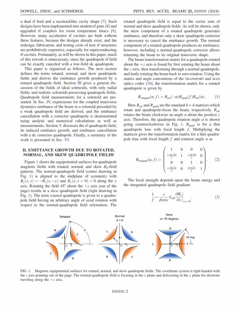
C. Multipole field measurements of a solenoid

Figure 2 shows magnetic measurements for the LCLS-Igun solenoid [14]. The upper plot is the z dependence of thelongitudinal field, as measured using a three-axis Hallprobe. The lower plot is the integrated quadrupole gradientand rotation angle as a function of z. The integratedquadrupole field gradient as measured by a short rotatingcoil is

Qmeas ≡ LcoilB2ðr ¼ rcoilÞ

rcoil: ð16Þ

Here Lcoil is the axial length of the rotating coil, rcoil isthe radius of the coil, and B2ðr ¼ rcoilÞ is the quadrupolefield at the coil’s radius.The rotating coil measurements show that quadrupole

fields peak at the ends of the solenoid as expected from theprevious discussion in Sec. III B. The data also show thatthe quadrupole angle changes 90° between the ends, whichcorresponds to a polarity reversal. In addition, the quadru-pole fields scale with the solenoid’s field. Therefore, theyqualify as anomalous quadrupole fields of the solenoid.These properties suggest that there is some magnetic

FIG. 2. Magnetic measurements of the LCLS gun solenoid foran integrated field of 0.046 T-m. Top: Hall probe measurementsof the solenoid axial field. The transverse location of themeasurement axis (the z axis) was determined by minimizingthe radial field. Bottom: Rotating coil measurements of thequadrupole field. The rotating coil dimensions were 2.5 cm longwith a 2.8 cm radius. The measured quadrupole field is thusaveraged over these dimensions.

DOWELL, ZHOU, and SCHMERGE PHYS. REV. ACCEL. BEAMS 21, 010101 (2018)

010101-4

material which is unintentionally within the solenoid’smagnetic field or quadrupolar coil winding error.In our experience, the sources of these low quadrupole

fields were difficult to identify and control even with state-of-the-art, finite-element-analysis calculations and follow-ing rigorous fabrication practices with a careful selection ofmaterials. Therefore, we decided to install weak normal andskew quadrupole correctors in the LCLS-I solenoid andoptimize their settings with the beam itself. Measurementsof the beam emittance taken while optimizing the quadru-pole correctors are described later in Sec. IV D.

IV. COUPLED TRANSVERSE DYNAMICS INQUADRUPOLE+SOLENOID SYSTEMS

In this section, we develop a simple yet accurate modelfor understanding the effects of a quadrupole and solenoidsystem with coupled transverse trajectories. These theo-retical studies and numerical simulations confirm that theemittance growth is due to well-defined coupled dynamicsbetween the transverse planes. In addition, the theory,

simulation, and experiments show that the emittancegrowth can be canceled with a correcting quadrupole field.In this theory, the full 4D transverse transport matrix

conserves the 4D emittance, since the transformation islinear in four dimensions. However, both the 2D subspacesof xx0 and yy0 can gain emittance because of nonzero crossterms in the beam matrix. The linear 4D transformationgenerates cross terms or correlations between the x and yplanes via nonzero off-diagonal beam matrix elements suchas Σxx0 Σxy , Σx0y, Σx0y0 , etc. Since a rotated quadrupole canalso create these cross terms, it is possible to use a correctorquadrupole to control them and the emittance they produce.

A. Emittance due to a quadrupole fieldnear the entrance of a solenoid

The emittance growth of a normal quadrupole followedby a solenoid is computed assuming a normal-quadrupolefield followed by a solenoid. The ðx; x0; y; y0Þ transforma-tion of a beam ray through a thin quadrupole lens followedby a solenoid can be written as [15]

RsolRquad ¼

0BBBBB@

cos2KL sinKLK sinKL cosKL sin2KL

K

−K sinKL cosKL cos2KL −Ksin2KL sinKL cosKL

− sinKL cosKL − sin2KLK cos2KL sinKL cosKL

K

Ksin2KL − sinKL cosKL −K sinKL cosKL cos2KL

1CCCCCA

0BBBBB@

1 0 0 0

− 1f 1 0 0

0 0 1 0

0 0 þ 1f 1

1CCCCCA: ð17Þ

Here L is the effective length of the solenoid, K ≡ eB0

2βγmc,B0 is the maximum interior magnetic field of the solenoid,and f is the focal length of the quadrupole field before thesolenoid. The beam is rotated through the angle KL by thesolenoid.As shown earlier, an initial 4 × 4 beam matrix Σð0Þ can

be transported through the quadrupole and solenoid pro-ducing the exit beam matrix Σð1Þ:

Σð1Þ ¼ RsolRquadΣð0ÞðRsolRquadÞT: ð18Þ

Using the same Σð0Þ for a perfectly parallel beam asbefore and working through tedious matrix algebra givesthe expected result for the transverse-plane emittancegrowth of a normal quadrupole followed by a solenoid as

ϵn;quadþsol ¼ βγσx;solσy;sol

fjsin 2KLj: ð19Þ

In other words, the emittance growth of a normalquadrupole followed by a solenoid is that of the quadrupolerotated the Larmor angle of the solenoid. The emittancegrowth is the same for both the x and y planes.Substituting the integrated quadrupole field for 1=f,

one finds the coupled transverse dynamics normalized

emittance growth depending only upon the beam size,the integrated quadrupole field, and the rotation angle of thebeam in the solenoid:

ϵn;quadþsol ¼ σx;solσy;soleQmc

jsin 2KLj: ð20Þ

Figure 3 compares this simple formula with a particletracking simulation for a solenoid preceded by a normal-quadrupole field. The initial beam had zero emittance andzero energy spread and was circular and uniform. No space-charge forces are included in the simulation. The figureshows the normalized emittances given by Eq. (19) and thesimulation, plotted as a function of the rms beam size at thesolenoid entrance. The normal-quadrupole focal length is50 m for a 6 MeV beam energy. This corresponds to anintegrated quadrupole field gradient of 4.3 G, which issimilar to the measured field of the LCLS solenoid (seeFig. 2). The analytic theory and the simulation assume ashort quadrupole field with this integrated quadrupole fieldlocated at the solenoid’s entrance. The simulation emittanceis slightly larger, since it includes both the coupled trans-verse dynamics emittance being discussed here andthe geometric aberration. The good agreement verifiesthe model’s assumptions and illustrates that even a weak,

EXACT CANCELLATION OF EMITTANCE GROWTH … PHYS. REV. ACCEL. BEAMS 21, 010101 (2018)

010101-5

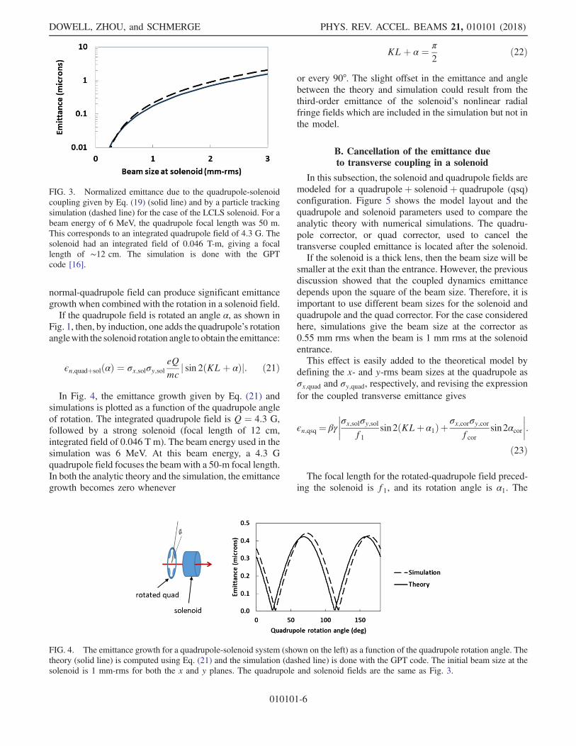
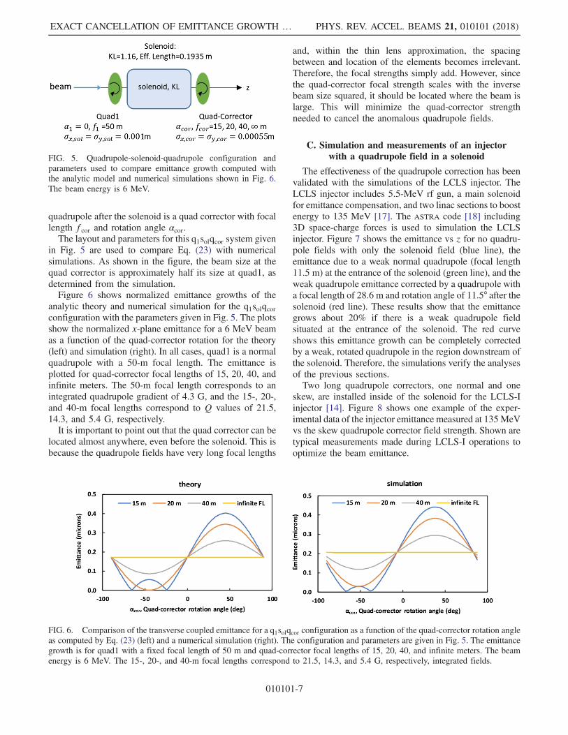
normal-quadrupole field can produce significant emittancegrowth when combined with the rotation in a solenoid field.If the quadrupole field is rotated an angle α, as shown in

Fig. 1, then, by induction, one adds the quadrupole’s rotationanglewith the solenoid rotation angle to obtain the emittance:

ϵn;quadþsolðαÞ ¼ σx;solσy;soleQmc

j sin 2ðKLþ αÞj: ð21Þ

In Fig. 4, the emittance growth given by Eq. (21) andsimulations is plotted as a function of the quadrupole angleof rotation. The integrated quadrupole field is Q ¼ 4.3 G,followed by a strong solenoid (focal length of 12 cm,integrated field of 0.046 T m). The beam energy used in thesimulation was 6 MeV. At this beam energy, a 4.3 Gquadrupole field focuses the beam with a 50-m focal length.In both the analytic theory and the simulation, the emittancegrowth becomes zero whenever

KLþ α ¼ π

2ð22Þ

or every 90°. The slight offset in the emittance and anglebetween the theory and simulation could result from thethird-order emittance of the solenoid’s nonlinear radialfringe fields which are included in the simulation but not inthe model.

B. Cancellation of the emittance dueto transverse coupling in a solenoid

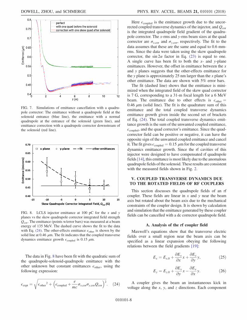
In this subsection, the solenoid and quadrupole fields aremodeled for a quadrupoleþ solenoidþ quadrupole (qsq)configuration. Figure 5 shows the model layout and thequadrupole and solenoid parameters used to compare theanalytic theory with numerical simulations. The quadru-pole corrector, or quad corrector, used to cancel thetransverse coupled emittance is located after the solenoid.If the solenoid is a thick lens, then the beam size will be

smaller at the exit than the entrance. However, the previousdiscussion showed that the coupled dynamics emittancedepends upon the square of the beam size. Therefore, it isimportant to use different beam sizes for the solenoid andquadrupole and the quad corrector. For the case consideredhere, simulations give the beam size at the corrector as0.55 mm rms when the beam is 1 mm rms at the solenoidentrance.This effect is easily added to the theoretical model by

defining the x- and y-rms beam sizes at the quadrupole asσx;quad and σy;quad, respectively, and revising the expressionfor the coupled transverse emittance gives

ϵn;qsq ¼ βγ

����σx;solσy;solf1sin2ðKLþα1Þþ

σx;corσy;corfcor

sin2αcor

����:ð23Þ

The focal length for the rotated-quadrupole field preced-ing the solenoid is f1, and its rotation angle is α1. The

FIG. 3. Normalized emittance due to the quadrupole-solenoidcoupling given by Eq. (19) (solid line) and by a particle trackingsimulation (dashed line) for the case of the LCLS solenoid. For abeam energy of 6 MeV, the quadrupole focal length was 50 m.This corresponds to an integrated quadrupole field of 4.3 G. Thesolenoid had an integrated field of 0.046 T-m, giving a focallength of ∼12 cm. The simulation is done with the GPTcode [16].

FIG. 4. The emittance growth for a quadrupole-solenoid system (shown on the left) as a function of the quadrupole rotation angle. Thetheory (solid line) is computed using Eq. (21) and the simulation (dashed line) is done with the GPT code. The initial beam size at thesolenoid is 1 mm-rms for both the x and y planes. The quadrupole and solenoid fields are the same as Fig. 3.

DOWELL, ZHOU, and SCHMERGE PHYS. REV. ACCEL. BEAMS 21, 010101 (2018)

010101-6

quadrupole after the solenoid is a quad corrector with focallength fcor and rotation angle αcor.The layout and parameters for this q1solqcor system given

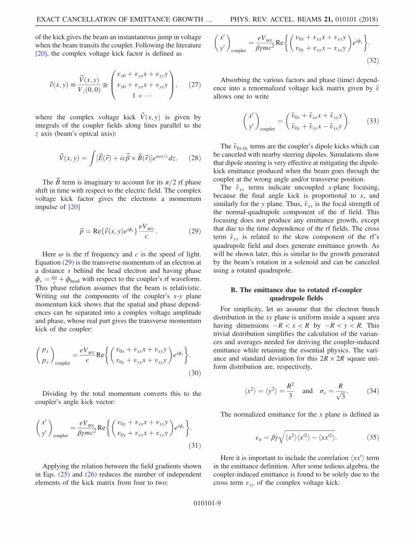
in Fig. 5 are used to compare Eq. (23) with numericalsimulations. As shown in the figure, the beam size at thequad corrector is approximately half its size at quad1, asdetermined from the simulation.Figure 6 shows normalized emittance growths of the

analytic theory and numerical simulation for the q1solqcorconfiguration with the parameters given in Fig. 5. The plotsshow the normalized x-plane emittance for a 6 MeV beamas a function of the quad-corrector rotation for the theory(left) and simulation (right). In all cases, quad1 is a normalquadrupole with a 50-m focal length. The emittance isplotted for quad-corrector focal lengths of 15, 20, 40, andinfinite meters. The 50-m focal length corresponds to anintegrated quadrupole gradient of 4.3 G, and the 15-, 20-,and 40-m focal lengths correspond to Q values of 21.5,14.3, and 5.4 G, respectively.It is important to point out that the quad corrector can be

located almost anywhere, even before the solenoid. This isbecause the quadrupole fields have very long focal lengths

and, within the thin lens approximation, the spacingbetween and location of the elements becomes irrelevant.Therefore, the focal strengths simply add. However, sincethe quad-corrector focal strength scales with the inversebeam size squared, it should be located where the beam islarge. This will minimize the quad-corrector strengthneeded to cancel the anomalous quadrupole fields.

C. Simulation and measurements of an injectorwith a quadrupole field in a solenoid

The effectiveness of the quadrupole correction has beenvalidated with the simulations of the LCLS injector. TheLCLS injector includes 5.5-MeV rf gun, a main solenoidfor emittance compensation, and two linac sections to boostenergy to 135 MeV [17]. The ASTRA code [18] including3D space-charge forces is used to simulation the LCLSinjector. Figure 7 shows the emittance vs z for no quadru-pole fields with only the solenoid field (blue line), theemittance due to a weak normal quadrupole (focal length11.5 m) at the entrance of the solenoid (green line), and theweak quadrupole emittance corrected by a quadrupole witha focal length of 28.6 m and rotation angle of 11.5° after thesolenoid (red line). These results show that the emittancegrows about 20% if there is a weak quadrupole fieldsituated at the entrance of the solenoid. The red curveshows this emittance growth can be completely correctedby a weak, rotated quadrupole in the region downstream ofthe solenoid. Therefore, the simulations verify the analysesof the previous sections.Two long quadrupole correctors, one normal and one

skew, are installed inside of the solenoid for the LCLS-Iinjector [14]. Figure 8 shows one example of the exper-imental data of the injector emittance measured at 135 MeVvs the skew quadrupole corrector field strength. Shown aretypical measurements made during LCLS-I operations tooptimize the beam emittance.

FIG. 5. Quadrupole-solenoid-quadrupole configuration andparameters used to compare emittance growth computed withthe analytic model and numerical simulations shown in Fig. 6.The beam energy is 6 MeV.

FIG. 6. Comparison of the transverse coupled emittance for a q1solqcor configuration as a function of the quad-corrector rotation angleas computed by Eq. (23) (left) and a numerical simulation (right). The configuration and parameters are given in Fig. 5. The emittancegrowth is for quad1 with a fixed focal length of 50 m and quad-corrector focal lengths of 15, 20, 40, and infinite meters. The beamenergy is 6 MeV. The 15-, 20-, and 40-m focal lengths correspond to 21.5, 14.3, and 5.4 G, respectively, integrated fields.

EXACT CANCELLATION OF EMITTANCE GROWTH … PHYS. REV. ACCEL. BEAMS 21, 010101 (2018)

010101-7

The data in Fig. 8 have been fit with the quadratic sum ofthe quadrupole-solenoid-quadrupole emittance with theother unknown but constant emittances ϵother, using thefollowing expression:

ϵexpt ¼ffiffiffiffiffiffiffiffiffiffiffiffiffiffiffiffiffiffiffiffiffiffiffiffiffiffiffiffiffiffiffiffiffiffiffiffiffiffiffiffiffiffiffiffiffiffiffiffiffiffiffiffiffiffiffiffiffiffiffiffiffiffiffiffiffiffiffiffiffiffiffiffiffiffiffiffiffiffiϵother

2 þ�ϵcoupled þ

emc

σx;corσy;corQcor

�2

r: ð24Þ

Here ϵcoupled is the emittance growth due to the uncor-rected coupled transverse dynamics of the injector, andQcoris the integrated quadrupole field gradient of the quadru-pole corrector. The x-rms and y-rms beam sizes at the quadcorrector are σx;cor and σy;cor, respectively. The fit to thedata assumes that these are the same and equal to 0.6 mm-rms. Since the data were taken using the skew quadrupolecorrector, the sin 2α factor in Eq. (23) is equal to one.A single curve has been fit to both the x- and y-planeemittances. However, the offset in emittance between the xand y planes suggests that the other-effects emittance forthe y plane is approximately 25 nm larger than the x plane’sother emittance. The data are shown with 5% error bars.The fit (dashed line) shows that the emittance is mini-

mized when the integrated field of the skew quad correctoris 7 G, corresponding to a 31-m focal length for a 6 MeVbeam. The emittance due to other effects is ϵother ¼0.46 μm (solid line). The fit is the quadrature sum of thisemittance and the total coupled transverse dynamicsemittance growth given inside the second set of bracketsof Eq. (24). The total coupled transverse dynamics emit-tance growth is the sum of the unwanted coupled emittance,ϵcoupled, and the quad corrector’s emittance. Since the quad-corrector field can be positive or negative, it can have theopposite sign of the unwanted coupled emittance and cancelit. The fit gives ϵcoupled ¼ 0.15 μm for the coupled transversedynamics emittance growth. Since the rf cavities of thisinjector were designed to have compensated rf quadrupolefields [14], this emittance ismost likely due to the anomalousquadrupole fields of the solenoid. These results are consistentwith the measured fields shown in Fig. 2.

V. COUPLED TRANSVERSE DYNAMICS DUETO THE ROTATED FIELDS OF RF COUPLERS

This section discusses the quadrupole fields of an rfcoupler. These fields are linear in x and y near the beamaxis but rotated about the beam axis due to the mechanicalconstraints of the coupler design. It is shown by calculationand simulation that the emittance generated by these couplerfields can be cancelled with a dc corrector quadrupole field.

A. Analysis of the rf coupler field

Maxwell’s equations show that the transverse electricfields over a small region near the beam axis can bespecified as a linear expansion obeying the followingrelations between the field gradients [19]:

Ex ¼ Ex;0 þ∂Ex

∂x xþ ∂Ex

∂y y; ð25Þ

Ey ¼ Ey;0 þ∂Ex

∂y x − ∂Ex

∂x y: ð26Þ

A coupler gives the beam an instantaneous kick involtage along the x, y, and z directions. Each component

FIG. 7. Simulations of emittance cancellation with a quadru-pole corrector: The emittance without a quadrupole field at thesolenoid entrance (blue line), the emittance with a normalquadrupole at the entrance of the solenoid (green line), andemittance correction with a quadrupole corrector downstream ofthe solenoid (red line).

FIG. 8. LCLS injector emittance at 100 pC for the x and yplanes vs the skew quadrupole corrector integrated field strengthQcor. The emittance (points w/error bars) was measured at a beamenergy of 135 MeV. The dashed curve shows the fit to the datawith Eq. (24). The other-effects emittance ϵother is shown by thesolid line at 0.46 μm. The fit indicates that the coupled transversedynamics emittance growth ϵcoupled is 0.15 μm.

DOWELL, ZHOU, and SCHMERGE PHYS. REV. ACCEL. BEAMS 21, 010101 (2018)

010101-8

of the kick gives the beam an instantaneous jump in voltagewhen the beam transits the coupler. Following the literature[20], the complex voltage kick factor is defined as

v⃗ðx; yÞ≡ V⃗ðx; yÞVzð0; 0Þ

≅

0B@

vx0 þ vxxxþ vxyy

vy0 þ vyxxþ vyyy

1þ � � �

1CA; ð27Þ

where the complex voltage kick V⃗ðx; yÞ is given byintegrals of the coupler fields along lines parallel to thez axis (beam’s optical axis):

V⃗ðx; yÞ ¼Z

½E⃗ðr⃗Þ þ icβ⃗ × B⃗ðr⃗Þ�eiωz=cdz: ð28Þ

The B⃗ term is imaginary to account for its π=2 rf phaseshift in time with respect to the electric field. The complexvoltage kick factor gives the electrons a momentumimpulse of [20]

p⃗ ¼ Refv⃗ðx; yÞeiϕsg eVacc

c: ð29Þ

Here ω is the rf frequency and c is the speed of light.Equation (29) is the transverse momentum of an electron ata distance s behind the head electron and having phaseϕs ¼ ωs

c þ ϕhead with respect to the coupler’s rf waveform.This phase relation assumes that the beam is relativistic.Writing out the components of the coupler’s x-y planemomentum kick shows that the spatial and phase depend-ences can be separated into a complex voltage amplitudeand phase, whose real part gives the transverse momentumkick of the coupler:

�px

py

�coupler

¼ eVacc

cRe

��v0x þ vxxxþ vxyy

v0y þ vyxxþ vyyy

�eiϕs

:

ð30Þ

Dividing by the total momentum converts this to thecoupler’s angle kick vector:

�x0

y0

�coupler

¼ eVacc

βγmc2Re

��v0x þ vxxxþ vxyy

v0y þ vyxxþ vyyy

�eiϕs

:

ð31Þ

Applying the relation between the field gradients shownin Eqs. (25) and (26) reduces the number of independentelements of the kick matrix from four to two:

�x0

y0

�coupler

¼ eVacc

βγmc2Re

��v0x þ vxxxþ vxyy

v0y þ vxyx − vxxy

�eiϕs

:

ð32Þ

Absorbing the various factors and phase (time) depend-ence into a renormalized voltage kick matrix given by ~vallows one to write

�x0

y0

�coupler

¼�~v0x þ ~vxxxþ ~vxyy

~v0y þ ~vxyx − ~vxxy

�: ð33Þ

The ~v0x;0y terms are the coupler’s dipole kicks which canbe canceled with nearby steering dipoles. Simulations showthat dipole steering is very effective at mitigating the dipole-kick emittance produced when the beam goes through thecoupler at the wrong angle and/or transverse position.The ~vxx terms indicate uncoupled x-plane focusing,

because the final angle kick is proportional to x, andsimilarly for the y plane. Thus, ~vxx is the focal strength ofthe normal-quadrupole component of the rf field. Thisfocusing does not produce any emittance growth, exceptthat due to the time dependence of the rf fields. The crossterm ~vxy is related to the skew component of the rf’squadrupole field and does generate emittance growth. Aswill be shown later, this is similar to the growth generatedby the beam’s rotation in a solenoid and can be canceledusing a rotated quadrupole.

B. The emittance due to rotated rf-couplerquadrupole fields

For simplicity, let us assume that the electron bunchdistribution in the xy plane is uniform inside a square areahaving dimensions −R < x < R by −R < y < R. Thistrivial distribution simplifies the calculation of the varian-ces and averages needed for deriving the coupler-inducedemittance while retaining the essential physics. The vari-ance and standard deviation for this 2R × 2R square uni-form distribution are, respectively,

hx2i ¼ hy2i ¼ R2

3and σx ¼

Rffiffiffi3

p : ð34Þ

The normalized emittance for the x plane is defined as

ϵn ¼ βγffiffiffiffiffiffiffiffiffiffiffiffiffiffiffiffiffiffiffiffiffiffiffiffiffiffiffiffiffiffiffiffiffiffihx2ihx02i − hxx02i

q: ð35Þ

Here it is important to include the correlation hxx0i termin the emittance definition. After some tedious algebra, thecoupler-induced emittance is found to be solely due to thecross term vxy of the complex voltage kick:

EXACT CANCELLATION OF EMITTANCE GROWTH … PHYS. REV. ACCEL. BEAMS 21, 010101 (2018)

010101-9

ϵn;couplerðsÞ ¼eVacc

mc2σ2x

����vrxy cos�ωsc

þ ϕhead

�

þ vixy sin

�ωsc

þ ϕhead

�����: ð36Þ

Here vrxy and vixy are the real and imaginary parts,respectively, of vxy.Equation (36) gives the transverse emittance of a thin

slice of the bunch, a distance s behind the bunch head. Therf phase of the bunch head is ϕhead, and the tail is a bunchlength, lbunch, behind it at the rf phase of ωlbunch

c þ ϕhead.Figure 9 shows as an example the head and tail emittancesvs the rf phase for a head-tail phase difference of 10 degrf.(Here the unit degrf is defined as one degree of phase atthe rf frequency of interest, which, in this case, is1.3 GHz.) The head minus the tail emittance is alsoplotted and shows that the difference is 20 nm or less,which is small compared to the uncorrected emittance ofmore than 100 nm; confirming the effect is mostly dueto the skewed quadrupole field rather than the phase-dependent kick.The emittance over the length of the bunch can be

computed by averaging the slice emittance in Eq. (36)over the longitudinal distribution of electrons. Assumingthe longitudinal distribution is uniform with full width,lbunch, then the bunch average emittance can be foundfrom

hϵn;coupleri ¼R lbunch0 ϵn;couplerðsÞdsR lbunch

0 ds: ð37Þ

Inserting the coupler slice emittance gives

hϵn;coupleri ¼eVacc

mc2σ2x

����vrxycos

�ωsc

þ ϕhead

��

þ vixy

sin

�ωsc

þ ϕhead

������: ð38Þ

Taking the averages and expanding in terms of the bunchlength gives the projected emittance of the bunch:

hϵn;coupleri¼eVacc

mc2σ2x

���ðvrxy cosϕheadþvixy sinϕheadÞ

− ðvrxy sinϕheadþvixy cosϕheadÞΔϕbunch

2

���: ð39Þ

The first term inside the absolute value function gives theemittance growth due to the rotated transverse quadrupolefield and generates emittance even for infinitesimal bunchlength. The second term depends linearly upon the bunchlength as well as the coupler’s skew field. For the shortbunches considered here Δϕbunch ≪ 1, and the second termcan be ignored, and the rf-coupler emittance growthbecomes

hϵn;coupleri ¼eVacc

mc2σ2xjvrxy cosϕhead þ vixy sinϕheadj: ð40Þ

It is important to note that, even if vxy ¼ 0, there remainsemittance growth from the normal-quadrupole term vxx,due the bunch’s phase length. The phase emittance occursbecause the rf field is time dependent. This changing fieldthen gives different quadrupole kicks along the bunchlength and generates projected emittance growth. The firstterm in Eq. (39) is absent for a normal-quadrupole rf field,since a normal-quadrupole has no emittance growth.However, the bunch length dependent term remains withvxy replaced by vxx. This emittance growth due to bunchlength can be mitigated by shaping the rf cavity [21] orintroducing additional penetrations into the cavity walls[22] to cancel both normal and skew components of thequadrupole rf field on the beam axis.

C. Cancellation of coupler kicks witha rotated quadrupole field

As shown in Sec. II, the kick angle vector in the xy planefor a quadrupole with focal length f and rotation angle αcan be written as

�x0

y0

�rotquad

¼�− cos 2α

f x − sin 2αf y

− sin 2αf xþ cos 2α

f y

�: ð41Þ

Comparing Eqs. (33) and (41), one can define the normaland skew components of the coupler’s quadrupole field:

FIG. 9. The head (s ¼ 0, solid line) and tail (ωstailc ¼ 10 degrf,dashed line) emittances vs phase for σx ¼ 1 mm. The emittancedifference in the head and tail (red line) is a maximum when thebeam is on the crest of the rf waveform. The coupler voltage andkick are Vacc ¼ 20 MV and vxy ¼ ð3.4þ 0.2iÞ × 10−6=mm,respectively, which are typical parameters for SRF cavities[20]. Here the unit degrf is a degree of phase at the rf frequencyof 1.3 GHz.

DOWELL, ZHOU, and SCHMERGE PHYS. REV. ACCEL. BEAMS 21, 010101 (2018)

010101-10

~vxx;coupler ¼ − cos2αcouplerfcoupler

and ~vxy;coupler ¼sin2αcouplerfcoupler

:

ð42Þ

Here the subscript ”coupler” has been added to denotethat these are kicks due to the rotated quadrupole field of arf coupler. These relations allow us to model the couplerfields equivalently as a quadrupole with focal length fcouplerand rotated αcoupler about the z axis. The rotation angle of

the coupler’s quadrupole field in terms of the normalizedvoltage kicks is

αcoupler ¼ − 1

2tan−1

~vxy~vxx

: ð43Þ

Since the quadrupole fields are weak, we can again applythe thin lens approximation and add Eqs. (33) and (41) togive the total kick angle of the coupler and a quad correctorlocated near the coupler:

�x0

y0

�total

¼�x0

y0

�coupler

þ�x0

y0

�quad

¼

0BB@

n~vxx − cos 2αcor

fcor

oxþ

n~vxy − sin 2αcor

fcor

oyn

~vxy − sin 2αcorfcor

ox −

n~vxx − cos 2αcor

fcor

oy

1CCA: ð44Þ

The symmetry of Maxwell’s equations, mentioned ear-lier in this section, can now be appreciated. Equation (44)proves that the emittance and the focusing effects of thecoupler can be exactly canceled with a rotated dc quadru-pole corrector. It shows that the following two equationsdetermine the quad-corrector focal strength and rotationangle which cancel the coupler quadrupole kick:

~vxx − cos 2αcorfcor

¼ 0 and ~vxy − sin 2αcorfcor

¼ 0. ð45Þ

Simultaneously solving these two equations gives pairedvalues for the quad corrector’s rotation angle and focalstrength which cancel the coupler field’s cross term(emittance) and the quadrupole-focus term (astigmatism)for a single slice of the bunch. Solutions for the quad-corrector rotation angle and focal strength are, respectively,

αcor ¼1

2tan−1

~vxy~vxx

; ð46Þ

1

fcor¼ eVacc

βγmc2

ffiffiffiffiffiffiffiffiffiffiffiffiffiffiffiffiffiffi~v2xx þ ~v2xy

q: ð47Þ

The normalized voltage kick factor ~v, in terms of thecomplex voltage kick factor v, is

~vxxðϕsÞ ¼eVacc

βγmc2ðvrxx cosϕs − vixx sinϕsÞ ð48Þ

and

~vxyðϕsÞ ¼eVacc

βγmc2ðvrxy cosϕs − vixy sinϕsÞ: ð49Þ

Inserting these relations into Eqs. (46) and (47) gives thequad-corrector rotation angle

αcorðϕsÞ ¼1

2tan−1

vrxy cosϕs − vixy sinϕs

vrxx cosϕs − vixx sinϕsð50Þ

and focal strength

1

fcorðϕsÞ¼ eVacc

βγmc2

ffiffiffiffiffiffiffiffiffiffiffiffiffiffiffiffiffiffiffiffiffiffiffiffiffiffiffiffiffiffiffiffiffiffiffiffiffiffiffiffiffiffiffiffiffiffiffiffiffiffiffiffiffiffiffiffiffiffiffiffiffiffiffiffiffiffiffiffiffiffiffiffiffiffiffiffiffiffiffiffiffiffiffiffiffiffiffiffiffiffiffiffiffiffiffiffiffiffiffiffiffiffiðvrxx cosϕs − vixx sinϕsÞ2 þ ðvrxy cosϕs − vixy sinϕsÞ2

q: ð51Þ

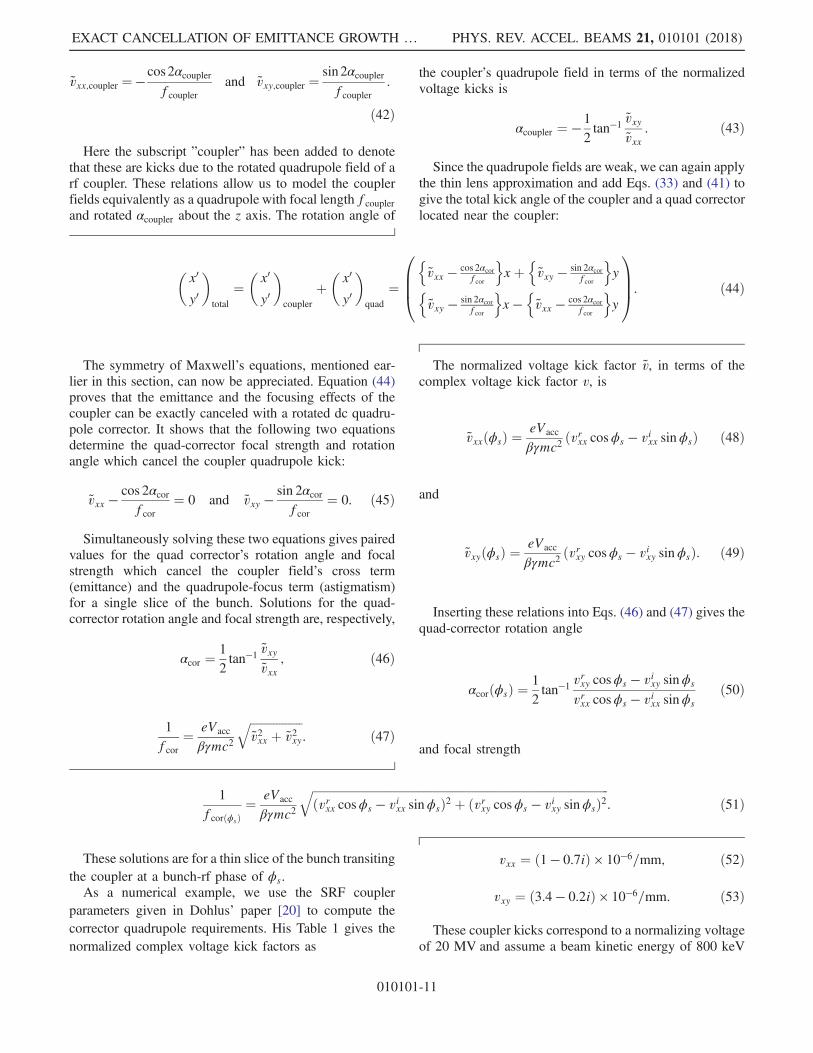
These solutions are for a thin slice of the bunch transitingthe coupler at a bunch-rf phase of ϕs.As a numerical example, we use the SRF coupler

parameters given in Dohlus’ paper [20] to compute thecorrector quadrupole requirements. His Table 1 gives thenormalized complex voltage kick factors as

vxx ¼ ð1 − 0.7iÞ × 10−6=mm; ð52Þ

vxy ¼ ð3.4 − 0.2iÞ × 10−6=mm: ð53Þ

These coupler kicks correspond to a normalizing voltageof 20 MV and assume a beam kinetic energy of 800 keV

EXACT CANCELLATION OF EMITTANCE GROWTH … PHYS. REV. ACCEL. BEAMS 21, 010101 (2018)

010101-11

such that βγ ¼ 2.5. Figure 10 shows the focal length androtation angle required to correct for these complex voltagekicks as functions of the beam-to-rf phase. The correctionquadrupole rotation angle and focal length are given asfunctions of the bunch’s head phase with respect to thecoupler rf waveform. A phase of 90 degrf corresponds tothe bunch head synchronized on the rf waveform crest.

D. Implementing quadrupole correctorsinto the LCLS-II injector

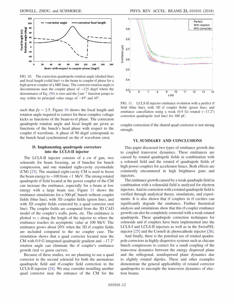
The LCLS-II injector consists of a cw rf gun, twosolenoids for beam focusing, an rf buncher for bunchcompression, and one standard eight-cavity cryomodule(CM) [23]. The standard eight-cavity CM is used to boostthe beam energy to∼100 from<1 MeV. The strong rotatedquadrupole rf field located at the power coupler of the CMcan increase the emittance, especially for a beam at lowenergy with a large beam size. Figure 11 shows theemittance simulations for a 300-pC bunch without couplerfields (blue line), with 3D coupler fields (green line), andwith 3D coupler fields corrected by a quad corrector (redline). The coupler fields are computed from the 3D CADmodel of the coupler’s walls, ports, etc. The emittance isplotted vs z along the length of the injector to where theemittance reaches its asymptotic value at 100 MeV. Theemittance grows about 20% when the 3D rf coupler fieldsare included compared to the no coupler case. Thesimulation shows that a quad corrector located near theCM with 0.9 G integrated quadrupole gradient and −17.2°rotation angle can eliminate the rf coupler’s emittancegrowth (red vs green curves).Because of these studies, we are planning to use a quad

corrector in the second solenoid for both the anomalousquadrupole field and rf-coupler field correction in theLCLS-II injector [24]. We may consider installing anotherquad corrector near the entrance of the CM for the

coupler correction if the shared quad corrector is not strongenough.

VI. SUMMARY AND CONCLUSIONS

This paper discussed two types of emittance growth dueto coupled transverse dynamics. These emittances arecaused by rotated quadrupole fields in combination witha solenoid field and the rotated rf quadrupole fields ofhigh power couplers for accelerator linacs. Both effects arecommonly encountered in high brightness guns andinjectors.The emittance growth caused by aweak quadruple field in

combination with a solenoidal field is analyzed for electroninjectors. And its correctionwith a rotated quadrupole field isverified through analytical theory, simulations, and experi-ments. It is also shown that rf couplers in rf cavities cansignificantly degrade the emittance. Further theoreticalanalysis and simulations show that this rf-coupler emittancegrowth can also be completely corrected with a weak rotatedquadrupole. These quadrupole correction techniques forsolenoids and rf couplers have been implemented into theLCLS-I and LCLS-II injectors as well as in the SwissFELinjector [25] and the Cornell dc photocathode injector [26].And finally, there is the potential use of rotated quadru-

pole correctors in highly dispersive systems such as chicanebunch compressors to correct for a small coupling of thetransverse dynamics between the energy dispersed planeand the orthogonal, nondispersed plane dynamics dueto slightly rotated dipoles. These and other examplesdemonstrate the general applicability of rotated correctorquadrupoles to uncouple the transverse dynamics of elec-tron beams.

FIG. 11. LCLS-II injector emittance evolution with a perfect rffield (blue line), with 3D rf coupler fields (green line), andemittance cancellation using a weak (0.9 G) rotated (−17.2°)correction quadrupole (red line) for 300 pC.

FIG. 10. The correction quadrupole rotation angle (dashed line)and focal length (solid line) vs the beam to coupler rf phase for ahigh-power coupler of a SRF linac. The corrector rotation angle isdiscontinuous near the coupler phase of ∼125 degrf where thedenominator of Eq. (50) is zero and the 1

2tan−1 function jumps to

stay within its principal value range of −45° and 45°.

DOWELL, ZHOU, and SCHMERGE PHYS. REV. ACCEL. BEAMS 21, 010101 (2018)

010101-12

ACKNOWLEDGMENTS

This work is supported by DOE under Grant No. DE-AC02-76SF00515. The authors also acknowledge the goodadvice of the journal’s anonymous referees. Their con-structive comments and suggestions motivated us to trans-form and improve the final paper.

[1] G. Ripken, Report No. DESY RI-70/5, 1970.[2] K. Wille, Report No. SLAC/AP-27, 1984.[3] H. Qin, R. C. Davidson, M. Chung, and J. W. Burby,

Generalized Courant-Snyder Theory for Charged-ParticleDynamics in General Focusing Lattices, Phys. Rev. Lett.111, 104801 (2013).

[4] H. Wiedemann, Particle Accelerator Physics II, Nonlinearand Higher-Order Beam Dynamics (Springer, New York,1995), Sec. 3.3.

[5] Z. Li, J. J. Bisognano, and B. C. Yunn, Transport Propertiesof the CEBAF Cavity, in Proceedings of the 15th ParticleAccelerator Conference, PAC-1993, Washington, DC, 1993(IEEE, New York, 1993) http://accelconf.web.cern.ch/accelconf/p93/PDF/PAC1993_0179.PDF.

[6] Z. Li, Ph.D. dissertation, College of William and Mary,1995.

[7] Z. Li, N. Folwell, L. Ge, A. Guetz, V. Ivanov, M. Kowalski,L.-Q. Lee, C. Ng, G. Schussman, L. Stingelin, R.Uplenchwar, M. Wolf, L. Xiao, and K. Ko, High perfor-mance computing in accelerating structure design andanalysis, Nucl. Instrum. Methods Phys. Res., Sect. A558, 168 (2006).

[8] L. Xiao, R. F. Boyce, D. H. Dowell, Z. Li, C. Limborg-Deprey, and J. Schmerge, Dual feed RF gun design for theLCLS, in Proceedings of the 21st Particle AcceleratorConference, Knoxville, TN, 2005 (IEEE, Piscataway,NJ, 2005), http://accelconf.web.cern.ch/AccelConf/p05/PAPERS/TPPE058.PDF.

[9] Z. Li, J. Chan, L. D. Bentson, D. H. Dowell, C. Limborg-Deprey, J. Schmerge, D. Schultz, and L. Xiao, Couplerdesign of the LCLS injector S-band structures, inProceedings of the 21st Particle Accelerator Conference,Knoxville, TN, 2005 (IEEE, Piscataway, NJ, 2005), http://accelconf.web.cern.ch/AccelConf/p05/PAPERS/TPPT031.PDF.

[10] D. C. Carey, K. L. Brown, and F. Rothacker, SLAC ReportNos. SLAC-R-530, Fermilab-Pub-98-310, and UC-414,pp. 148.

[11] K. T. McDonald, Expansion of an axially symmetric,static magnetic field in terms of its axial field,http://physics.princeton.edu/∼mcdonald/examples/axial.pdf(unpublished).

[12] D. H. Dowell, Sources of emittance in rf photocathodeinjectors: Intrinsic emittance, space charge forces due tonon-uniformities, arXiv:1610.01242.

[13] D. C. Carey, K. L. Brown, and F. Rothacker, SLAC ReportNos. SLAC-R-530, Fermilab-Pub-98-310, and UC-414,p. 127.

[14] D. H. Dowell, E. Jongewaard, J. Lewandowski, C.Limborg-Deprey, Z. Li, J. Schmerge, A. Vlieks, J. Wang,and L. Xiao, Report No. SLAC-Pub-13401,arXiv:1503.05877.

[15] D. C. Carey, K. L. Brown, and F. Rothacker, SLAC ReportNos. SLAC-R-530, Fermilab-Pub-98-310, and UC-414,p. 161.

[16] GPT: General Particle Tracer, version 2.82, Pulsar Physics,http://www.pulsar.nl/gpt/.

[17] R. Akre, D. Dowell, P. Emma, J. Frisch, S. Gilevich, G.Hays, Ph. Hering, R. Iverson, C. Limborg-Deprey, H.Loos, A. Miahnahri, J. Schmerge, J. Turner, J. Welch, W.White, and J. Wu, Commissioning the Linac CoherentLight Source injector, Phys. Rev. ST Accel. Beams 11,030703 (2008).

[18] K. Floettmann, ASTRA manual, DESY, Germany, 2017,http://www.desy.de/∼mpyflo/Astra_manual/Astra-Manual_V3.2.pdf (unpublished).

[19] D. H. Dowell, SLAC Pubs Report No. LCLS-II-TN-15-05[arXiv:1503.09142].

[20] M. Dohlus, I. Zagorodnov, E. Gjonaj, and T. Weiland,Coupler kick for very short bunches and its compensation,in Proceedings of the 11th European Particle AcceleratorConference, Genoa, 2008 (EPS-AG, Genoa, Italy, 2008),pp. 580–582, http://accelconf.web.cern.ch/AccelConf/e08/papers/mopp013.pdf.

[21] Z. Li, F. Zhou, A. Vlieks, and C. Adolphsen, On theimportance of symmetrizing RF coupler fields for lowemittance beams, in Proceedings of the 24th ParticleAccelerator Conference, PAC-2011, New York, 2011(IEEE, New York, 2011), pp. 2044–2046, http://accelconf.web.cern.ch/AccelConf/PAC2011/papers/thoas1.pdf.

[22] M. S. Chae, J. H. Hong, Y.W. Parc, In Soo Ko, S. J. Park,H. J. Qian, W. H. Huang, and C. X. Tang, Emittancegrowth due to multipole transverse magnetic modes inan rf gun, Phys. Rev. STAccel. Beams 14, 104203 (2011).

[23] LCLS-II Final Design Report, 2016, p. 49, https://docs.slac.stanford.edu/sites/pub/Publications/LCLSII%20Final_Design_Report.pdf.

[24] F. Zhou, D. Dowell, R. K. Li, T. O. Raubenheimer, J.Schmerge, C. Mitchell, C. Papadopoulos, F. Sannibale,and A. Vivoli, LCLS-II injector beamline design and RFcoupler correction, inProceedings of the 2015 InternationalFEL Conference, Daejeon, Korea, http://accelconf.web.cern.ch/AccelConf/FEL2015/papers/mop021.pdf.

[25] T. Schietinger, M. Pedrozzi, M. Aiba, V. Arsov, S. Bettoni,B. Beutner, M. Calvi, P. Craievich, M. Dehler, F. Frei, R.Ganter, C. P. Hauri, R. Ischebeck, Y. Ivanisenko, M.Janousch, M. Kaiser, B. Keil, F. Löhl, G. L. Orlandi, C.Ozkan Loch, P. Peier, E. Prat, J.-Y. Raguin, S. Reiche, T.Schilcher, P. Wiegand, E. Zimoch, D. Anicic, D.Armstrong, M. Baldinger, R. Baldinger, A. Bertrand,K. Bitterli, M. Bopp, H. Brands, H. H. Braun, M.Brönnimann, I. Brunnenkant, P. Chevtsov, J. Chrin, A.Citterio, M. Csatari Divall, M. Dach, A. Dax, R. Ditter, E.Divall, A. Falone, H. Fitze, C. Geiselhart, M.W.Guetg, F. Hämmerli, A. Hauff, M. Heiniger, C. Higgs,W. Hugentobler, S. Hunziker, G. Janser, B. Kalantari, R.Kalt, Y. Kim, W. Koprek, T. Korhonen, R. Krempaska, M.

EXACT CANCELLATION OF EMITTANCE GROWTH … PHYS. REV. ACCEL. BEAMS 21, 010101 (2018)

010101-13

Laznovsky, S. Lehner, F. Le Pimpec, T. Lippuner, H. Lutz,S. Mair, F. Marcellini, G. Marinkovic, R. Menzel, N. Milas,T. Pal, P. Pollet, W. Portmann, A. Rezaeizadeh, S. Ritt, M.Rohrer, M. Schär, L. Schebacher, St. Scherrer, V. Schlott,T. Schmidt, L. Schulz, B. Smit, M. Stadler, B. Steffen, L.Stingelin, W. Sturzenegger, D. M. Treyer, A. Trisorio, W.Tron, C. Vicario, R. Zennaro, and D. Zimoch,

Commissioning experience and beam physics measure-ments at the SwissFEL Injector Test Facility, Phys. Rev.Accel. Beams 19, 100702 (2016).

[26] A. Bartnik, C. Gulliford, I. Bazarov, L. Cultera, and B.Dunham, Operational experience with nanocoulomb bunchcharges in the Cornell photoinjector, Phys. Rev. ST Accel.Beams 18, 083401 (2015).

DOWELL, ZHOU, and SCHMERGE PHYS. REV. ACCEL. BEAMS 21, 010101 (2018)

010101-14