Policy gradient methods for free-electron laser and terahertz sourceoptimization and stabilization at the FERMI free-electron laser at Elettra

F. H. O’Shea,1,*,† N. Bruchon ,2 and G. Gaio11Elettra Sincrotrone Trieste, 34149 Trieste, Italy

2University of Trieste, 34127 Trieste, Italy

(Received 25 July 2020; accepted 3 December 2020; published 21 December 2020)

In this article we report on the application of a model-free reinforcement learning method to theoptimization of accelerator systems. We simplify a policy gradient algorithm to accelerator control fromsophisticated algorithms that have recently been demonstrated to solve complex dynamic problems. Afteroutlining a theoretical basis for the functioning of the algorithm, we explore the small hyperparameterspace to develop intuition about said parameters using a simple number-guess environment. Finally, wedemonstrate the algorithm optimizing both a free-electron laser and an accelerator-based terahertz sourcein-situ. The algorithm is applied to different accelerator control systems and optimizes the desired signalsin a few hundred steps without any domain knowledge using up to five control parameters. In addition,the algorithm shows modest tolerance to accelerator fault conditions without any special preparation forsuch conditions.

DOI: 10.1103/PhysRevAccelBeams.23.122802

I. INTRODUCTION

In this work we demonstrate a simple model-freereinforcement learning algorithm tuning and maintainingaccelerator systems. Herein, we simplify a policy gradientalgorithm related to those that have recently been demon-strated solving the complex, dynamic problem of playinghuman players in video games [1,2]. The algorithm is noisetolerant, requires little training beforehand, has few hyperparameters, and produces both a point estimate and anuncertainty estimate for all of the controlled systems. Inaddition, the algorithm natively adjusts the precision ofthe systems settings; and has demonstrated a tolerance forshort system shut downs in some cases. In this article, wedescribe the algorithm and how we arrived at it, show asimple simulation method for selecting the hyper param-eter, and show it operating several different acceleratorsubsystems.The success of accelerators is, in part, judged by the

science output and a key factor in output is the timespent serving the users. Because of this, any tuning doneonline places a premium on fast learning, whether byhuman operators or computer systems. In this context, we

demonstrate a simplified policy gradient method [3], a typeof reinforcement learning algorithm, tuning and maintain-ing a free-electron laser and a terahertz source. Algorithmswithin this family have recently shown the ability toperform complex tasks with extensive training [1,2]. Ourgoal is to decrease the number of steps to convergence inthe somewhat simpler realm of accelerator control.As computing power has proliferated in recent decades, a

variety of computer-based tools have been developed toimprove a machine setting or maintain performance [4–9].Among the more recent of these tools are methods basedon machine learning (ML). In addition to machine tuningand control, ML models can also be used to create newdiagnostics [10]. The majority of the applications of ML toaccelerators are based on supervised learning, where adataset with labeled outputs is used to fit a model to produceoutputs using novel data. A drawback to these methods is therequired labeled dataset. Without a dataset, the model cannotbe trained. Or, even so, the dataset may not cover the desiredoperational range or be too noisy and the model may bepoorly fit in regions of operational interest.An approach to mitigating this problem is to use the

information available to set the accelerator in approxi-mately the correct fashion and then tune it from there.Indeed, this is standard practice at all accelerator facilities,even when humans tune the accelerator. Presumably theinitial setting was not random and a superior setting mightbe found in the local parameter-space by either manualtuning [11], automatic feedbacks [4], random search [6], orsome other optimization technique [5–8]. Similar to thesetypes of algorithms, reinforcement learning might be

*finn.h.oshea@gmail.com†Present address: Nusano Inc., 28575 Livingston Ave, Valencia,

California 91355, USA.

Published by the American Physical Society under the terms ofthe Creative Commons Attribution 4.0 International license.Further distribution of this work must maintain attribution tothe author(s) and the published article’s title, journal citation,and DOI.

PHYSICAL REVIEW ACCELERATORS AND BEAMS 23, 122802 (2020)

2469-9888=20=23(12)=122802(20) 122802-1 Published by the American Physical Society

used to explore the parameter space and find a bettersolution [12].Reinforcement learning (RL) is a machine learning

paradigm in which an agent is allowed to take action inan environment in which it receives rewards for performingdesired behavior while it follows a policy. The goal ofreinforcement learning is to find an optimal policy to followand a distinguishing feature of reinforcement learning ascompared to supervised learning is that it requires the agentto interact with the environment, rather than learn from a setof labeled data. The optimal policy is typically defined asthe policy that produces the largest reward. In the contextof accelerator operations, the agent is a piece of controlsoftware and the environment is the accelerator itself. Thedefinitions of the other elements depends on what exactlythe agent is doing. For example, the actions might be toadjust the settings of steering magnets to improve theenergy output of a free-electron laser which is used tocompute a reward.In Sec. II we describe why we decided to work with

reinforcement learning agents at FERMI. In Sec. III webriefly review policy gradient methods; we also describethe specific algorithm we use in the present work. Thesoftware used in this work was written entirely by theauthors in python 3 [13], using available scientific libraries[14]. In Sec. IV we describe the types of policies weconsider for deployment at the accelerator. In Sec. V we usea fast numerical simulation to guide the selection of thepolicy type and hyperparameter settings. In Sec. VI wedemonstrate the algorithm performing various tasks on anFEL and THz source. We conclude with some remarks onthe performance of the algorithm.

II. WHY USE REINFORCEMENT LEARNINGAT FERMI?

The principal reason we have decided to use reinforce-ment learning, instead of supervised learning, is that ourwork with supervised learning showed that the learningwould have to be continuous.The operational conditions at FERMI are such that the

FEL is typically reconfigured for a new user twice perweek. The changes include everything from the undulatorsettings to the beam energy which can involve activating ordeactivating klystrons. For every new run the acceleratorphysics team retunes the machine, frequently starting at theelectron gun and working all the way to the beam dump. Itis not unusual for the retuning process to alter the setting ofdozens of features: power supply settings, klystron phases,and so on. Some configurations are used for less than aweek and are not reused for months or years.This situation creates a sparsity of data for training

supervised learning models. Every time the accelerator isretuned, the machine learning model is likely to needretraining, with all previous information rendered poten-tially useless. Every time the accelerator is tuned to a

configuration that the machine learning model has neverbeen exposed to, the model must certainly be retrained.Taken a whole, these aspects of operations at FERMI meanthat the model would probably have to be retrained severaltimes a week, at least.However, even this is a somewhat optimistic assessment

of the longevity of the value of asynchronous training atFERMI. We would regularly find that the ability of atrained model to predict other features of the acceleratorwould decay in less than an hour. We show an example ofthe reduction in the model performance as a function oftime in Fig. 1. To make the prediction model we use libraryfunctions from scikit-learn [15] to build a neural networkwith 2 hidden layers of size 100 and tanh activationfunction. The task is for the agent to predict the FELintensity as measured by the intensity monitor [16]. Thisdata was taken while FEL1 was in HGHG operation [17].The 162 features used in the model are taken from the

entire accelerator from the photocathode laser to the beamdump. No features from the photon transport line were used

FIG. 1. Prediction performance of a neural network model atFERMI. The model uses several hundred features along the linacand FEL to predict the output intensity of the FERMI FEL. TheR2 score on the training set is shown as a circle, the score is 0.995.The score on the cross validation set is shown as a square, thescore is 0.914. The x-marks show the R2 score for the model as afunction of time after the first training sample was taken. Thesamples are accumulated in batches of approximately 1000 andthe score is computed for each batch. Before each batch is scored,any sample with any feature value greater than 5 standarddeviations from the mean for that batch is removed. The shadedregion beginning at approximately 10 minutes shows a period oftime when Klystron #3 went in to fault and the accelerator wasnot running.

F. H. O’SHEA, N. BRUCHON, and G. GAIO PHYS. REV. ACCEL. BEAMS 23, 122802 (2020)

122802-2

as they are very strongly correlated with the FEL intensityand it seemed to us to defeat the purpose of the task if wewere to use photon beam measurements to predict photonbeam properties. The features include: BPM readings alongthe whole accelerator, corrector magnet settings insideFEL1, various properties of the photocathode, laser heaterand seed lasers (position, intensity, delay, etc.), the bunchcharge measured at the beam dump, the time of arrival ofthe bunch at the bunch linearizer, and the pyro reading ofthe bunch length.The accelerator and FEL were left to run with the

feedbacks on for approximately 30 minutes, wherein wetook approximately 27000 data points. The data was takenusing a data collection system at FERMI that is asynchro-nous and has to be operated by the user manually. Because ofthese constraints, the data points are not spread out evenlyover the 30 minute interval. However, the data covers thetime period sufficiently well for our purposes here.The training and model evaluation were performed

offline. The neural network is trained on the first 5000data points (approximately 10 minutes worth of data), andthe next 1000 points are used as a cross-validation set forhyperparameter scans and selection. After this time period,the remaining points are grouped into sets of approximately1000 and scored. The scoring system used is the so-calledcoefficient of determination (R2) which is computed as

R2 ¼ 1 −P

iðyi − fiÞ2Piðyi − yÞ2 : ð1Þ

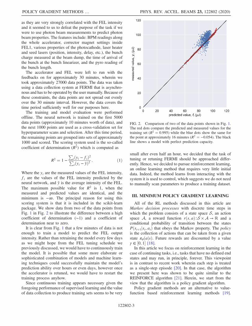
Where the yi are the measured values of the FEL intensity,fi are the values of the FEL intensity predicted by theneural network, and y is the average intensity of the FEL.The maximum possible value for R2 is 1, when themeasured and predicted values are identical, and theminimum is −∞. The principal reason for using thisscoring system is that it is included in the scikit-learnpackage. We show data from two of the data points fromFig. 1 in Fig. 2 to illustrate the difference between a highcoefficient of determination (∼1) and a coefficient ofdetermination near to zero.It is clear from Fig. 1 that a few minutes of data is not

enough to train a model to predict the FEL outputintensity. Rather than retraining the model every few daysas we might hope from the FEL tuning schedule wepreviously discussed, we would have to continuously trainthe model. It is possible that some more elaborate orsophisticated combination of models and machine learn-ing techniques could successfully maintain the model’sprediction ability over hours or even days, however oncethe accelerator is retuned, we would have to restart thetraining process anyhow.Since continuous training appears necessary given the

foregoing performance of supervised learning and the valueof data collection to produce training sets seems to be very

small after even half an hour, we decided that the task oftuning or retuning FERMI should be approached differ-ently. Hence, we decided to pursue reinforcement learning,an online learning method that requires very little initialdata. Indeed, the method learns from interacting with thesystem it is used to control, which suggests we do not needto manually scan parameters to produce a training dataset.

III. MINIMUM POLICY GRADIENT LEARNING

All of the RL methods discussed in this article areMarkov decision processes with discrete time steps inwhich the problem consists of a state space S, an actionspace A, a reward function rðs; aÞ∶S ×A → R and aconditional probability of transition between the statesPðstþ1jst; atÞ that obeys the Markov property. The policyis the collection of actions that can be taken from a givenstate πθðajsÞ. Future rewards are discounted by a valueγ ∈ ½0; 1� [18].In this article we focus on reinforcement learning in the

case of continuing tasks, i.e., tasks that have no defined endstates and may run, in principle, forever. This viewpointis in contrast to recent work wherein each step is treatedas a single-step episode [20]. In that case, the algorithmwe present here was shown to be quite similar to theREINFORCE algorithm [21]. Herein, we start from theview that the algorithm is a policy gradient algorithm.Policy gradient methods are an alternative to value-

function based reinforcement learning methods [19].

FIG. 2. Comparison of two of the data points shown in Fig. 1.The red dots compare the predicted and measured values for thetraining set (R2 ¼ 0.995) while the blue dots show the same forthe point at approximately 16 minutes (R2 ¼ −0.054). The blackline shows a model with perfect prediction capacity.

POLICY GRADIENT METHODS … PHYS. REV. ACCEL. BEAMS 23, 122802 (2020)

122802-3

Briefly, value-function based methods estimate the value ofthe states partially by using the value of the subsequentstates, the desired behavior from the agent is then to visitthe high value states as often as possible, and, from thealgorithm designer’s perspective, achieve convergence asquickly as possible. Perhaps the most well-known exampleof a value-function based-RL method is deep Q-learningwith neural networks [22]. This RL algorithm uses functionapproximation to adapt an off-policy tabular learningmethod to problems where the number of state-action pairsis large. The actions at each step are chosen from a finite listof options that may be state-dependent via the epsilon-greedy method [23]. A shortcoming of deep Q-learning isthat the policy improvement theorem, that Q-learning relieson to guarantee convergence, no longer applies whenfunction approximation is used [19].Alternatively, policy gradient methods parametrizes a

continuous policy for the actions. This has a number ofadvantages over value-function based methods: (1) thepolicy can be fundamentally stochastic and we do not needto include off-policy techniques or variably greedy actionchoices (such as epsilon-greedy) to allow or encourageexploration of the action space; (2) the policy can, inprinciple, become deterministic, if that is what the envi-ronment rewards; (3) policies are usually what we areinterested in, i.e., when the accelerator is in a certain statewe want the agent to take certain actions, and by definingthe policy we have the ability to incorporate acceleratordomain knowledge in the definition of the policy; (4) con-vergence to (at least) a local optimum is guaranteed [19].Some examples of how accelerator domain knowledge

might be used to choose or constrain a policy for the agentare as follows. If the designer knows that turning a certaindipole down too low will cause unacceptable beam losses,they can prohibit the policy that the agent controls thatdipole with from becoming too low. This way, the agentdoes not have to learn from the negative feedback of beamloss. Another example is if a particular beam line uses aquadrupole doublet. It might be useful for the doubletcondition (equal and opposite gradients in the two quadru-poles) to be relaxed, but not entirely. In this case thedesigner could ensure the policies of the two magnets arecorrelated. The strength of the correlation could itself be alearned parameter.Policy gradient methods rely on optimizing the average

expected discounted reward the agent receives over a horizon,h, which is the number of steps into the “future” that are usedin estimating the expected discounted reward [24]

Jt ≐ E

�1

h

Xhu¼1

γu−1rtþu

�¼ 1

h

Xhu¼1

γu−1Ea∼πtþus∼ptþu

½rtþu�

¼ 1

h

Xhu¼1

γu−1ZS

ZArðs; aÞptþuðs; aÞdads; ð2Þ

where t is an arbitrary step number and the expression for theaverage expected discounted reward at the next step is

Jtþ1 ¼1

h

Xhu¼1

γu−1ZS

ZArðs; aÞptþuþ1ðs; aÞdads: ð3Þ

The interpretation of pnðs; aÞ is the joint probability thatthe agent will visit the state s and take action a on step n andwe see that it can change at every step, as is indicated by thesubscript to p. Practically, the value for h is arbitrary andthe sum can be truncated when the hþ 1 discounted futurereward is small compared to the sum of the previousrewards. Formally, h can be infinite so long as we do notalso have γ ¼ 1. If γ ¼ 1, then the system must reach aterminal state for the reward to be finite, in which case h isthe number of steps until a terminal state. This would makethe solution a Monte Carlo policy gradient method [19,21].However, we are here focusing on continuing tasks, and donot pursue this further.The policy is updated, in principle, using gradient ascent

such that

θtþ1 ¼ θt þ α∇θJtðθÞ; ð4Þ

where θ is the set of policy parameters that the agentcontrols, and α is the learning rate. In order to computethis, we need to obtain a relationship between Jt and theagent’s policy.If we change the agent’s behavior at step tþ 1, we

expect that J might change: Jtþ1 ¼ Jt þ ΔJ. CombiningEqs. (2) and (3) we find a way to compute the quantity weneed as

ΔJ ¼ 1

h

ZSds

ZAdarðs; aÞ

�ð1 − γÞ

Xh−1u¼1

γu−1ptþuþ1ðs; aÞ

þ γh−1ptþhþ1ðs; aÞ − ptðs; aÞ�: ð5Þ

If we know how p changes as a function of step number,we can compute the change in J, but we do not usuallyknow p. For the purposes of the present work we make theassumption that agent changes its policy at step tþ 1 andthen follows it until it has taken at least h more steps in theMDP. With this assumption, we find that

ΔJ ¼ 1

h

ZSds

ZAdarðs; aÞ

× ½πtþ1ðajsÞutþ1ðsÞ − πtðajsÞutðsÞ�: ð6Þ

Where we have used the identity ptðs; aÞ ¼ πtðajsÞutðsÞ,where πtðajsÞ is the policy at step t (the probability oftaking action a from state s) and utðsÞ is the probabilitydistribution of states, s, at step t. We note that the discount

F. H. O’SHEA, N. BRUCHON, and G. GAIO PHYS. REV. ACCEL. BEAMS 23, 122802 (2020)

122802-4

factor has disappeared and that h is now an arbitraryconstant [25]. This equation is still difficult to use unlesswe know the probability of visiting the states. To furthersimplify the computation we might assume that utþ1ðsÞ ¼utðsÞ, as is assumed for policy gradient methods [19].In that case, since the policy is parametrized by θ we canwrite the update rule for the parameters as

θtþ1 ≈ θt þ αEa∼πθs∼u

½rðs; aÞ∇θ ln ðπθðajsÞÞ�; ð7Þ

where h has been absorbed in to the learning rate. This is arestatement of the policy gradient theorem [3].The validity of the last assumption is dubious because

the goal of learning is to find a policy that takes the agent tohigher-value states and thusly produces higher averagereturn. On the other hand, the equality is approximatelytrue if the change in policy is small. This is generally usefulbut might limit how quickly the agent can learn and updateits policy.An unrelated difficulty with this method is that it must

calculate an expectation value in Eq. (7). We can reduce thecomputational complexity by approximating Eq. (7) usingstochastic gradient ascent

θtþ1 ≈ θt þ αrðs; aÞ∇θ ln ðπθðajsÞÞ: ð8Þ

The convergence properties of Eq. (8) can be improved ifthe gradient is performed with respect to the Fisher metricrather than directly in parameter space, in which casewe take ∇θ → IðθÞ−1∇θ in the preceding equations, whereIðθÞ−1 is the inverse of the Fisher matrix [26]. This is theupdate formula we use in this work.Previously we had assumed that the changes to the

distribution of states with policy changes was negligibleand used that to develop an update rule for the policyparameters. But there is one case in which the distributionof states is always steady, regardless of the size of policychanges: if there is only one state. Not only does theassumption of a single state allow us this improvement tothe theoretical basis of policy improvement, but it has otherbenefits as well. It also obviates the need for a definition ofstates of the accelerator and increases the density ofrewards because they all accrue to that single state. Bothof these features should decrease the number of stepsrequired to learn the optimal policy. The cost is that theagent does not store any information about actions that arenot available in the current policy. If the agent is sufficientlyfast at learning, this drawback may be worth the cost.Because we are working with a single state, we note that thetransition probability mentioned earlier, Pðstþ1jst; atÞ ¼ 1,is deterministic.The algorithm we used is based on the continuing actor-

critic method with eligibility traces of Sutton and Barto[19]. We chose a continuing algorithm because there wasno clear way to define an end state for the accelerator

environment. In addition, as there is only one state, we didnot use the critic. The motivation for making this change isstraightforward, if naïve: we did not want to spend valuabletraining time learning the value of the state. This changewould not be possible with state-based methods, but policygradient methods require only a parametrized policy and donot require states. We call the algorithm minimum policygradient learning and it is shown in Algorithm 1.The algorithm proceeds as follows. The user chooses a

policy distribution to use and then computes the associatedgradient and Fisher Information Matrix (examples of theseelements are given in Sec. IV). The users also selects valuesfor the learning rate for the parameters (α), the learningrate for the base line (αR), and the strength of the eligibilitytrace (λθ). All other parameters are initialized to arbitraryvalues [27]. On line 7 of Algorithm 1, the policy is sampledto return a specific action. Next, that action is taken by theagent who receives a reward (details on rewards we usedcan be found in Secs. Vand VI) and that reward is adjustedfor the baseline (line 9). On line 10 the baseline is updatedusing gradient ascent. Next, the eligibility trace vector isupdated on line 11. Finally, the parameters are updatedusing gradient ascent.In fact, because there is only one state, the base line, R in

Algorithm 1, can serve as a kind of critic. However, wefound that the baseline slowed learning because it rewardedthe agent too generously for simply taking actions withbetter-than-baseline reward. Because of this, we have usedαR ¼ 0 in all of the simulations and accelerator control testspresented in this work.Whether the trade-off between density of reward and the

more detailed information about the accelerator stored by alarger number of states is worthwhile is beyond the scope ofthe present work. However, we make a few observationshere. First, if the accelerator parameter space is large, and itusually is, and the accelerator is unlikely to revisit a stateoften, then the agent is unlikely to make use of theinformation anyway. Second, large parameter spacesrequire careful generalization techniques to ensure thatthe information is not “spread so far” that the agent is

Algorithm 1. Minimum Policy Gradient Learning.

1 Input: Policy distribution, Fisher matrix and gradient2 Algorithm parameters: α, αR, λθ3 Initialize the model parameters, θ ← 04 Initialize the eligibility trace vector, z ← 05 Initialize the base line, R ¼ 06 While True:7 A ∼ πð·jθÞ8 Take action A, observe reward R9 δ ← R − R10 R ← Rþ αRδ11 z ← λθzþ IðθÞ−1∇ ln πðAjθÞ12 θ ← θ þ αδz

POLICY GRADIENT METHODS … PHYS. REV. ACCEL. BEAMS 23, 122802 (2020)

122802-5

treating different states of the accelerator as the same state.Third, it is not clear that the list of features currentlymeasured and recorded at, for example, FERMI, is suffi-cient to distinguish between different accelerator states. Forexample, the best diagnostic for the strength of the micro-bunching instability [28] at FERMI is the FEL itself, and soa fundamental feature to the performance of the FEL is onlyknown to the agent through the rewards it receives. Thatinformation is stored in the policy that the agent learns andnot in the state, and it is not clear how to define a state suchthat it encodes that information. Presumably that informa-tion might be emergent; the agent might learn to control themicrobunching instability through some complex combi-nation of control parameters that are as-yet too contrivedfor a human operator.Finally, we note a potential cost to the single-state

assumption of our model. With only a single state, it seemslikely that model will not respond well to sufficiently fastand large changes to the accelerator. There is someevidence that this is the case in our present work asdemonstrated in the mixed results with respect to recoveryfrom faults or user perturbation of the system beingcontrolled, e.g., in Figs. 9 and 11. But it is also not yetclear what changes to the model would improve the agent’sperformance and how many resources those changes wouldrequire to be successful.As a heuristic for selecting which systems this algorithm

might successfully control, we asked ourselves a question:will changes in the accelerator state, as modeled by theinput to any arbitrary control algorithm, require that thealgorithm take very different actions faster than it canlearn? If yes, then a reinforcement algorithm will likelyneed to use state representations as a way to differentiatebetween the different control situations it encounters. If no,then a single-state might suffice. Examples of subsystemsthat might be controlled well by our single state algorithmare beam trajectory control, temperature stabilization(cryogenic or otherwise), maintaining rf system parametersagainst drift, fine tuning of undulator gaps in a chain ofundulators, or optimizing the laser spot profile on a photo-cathode. During normal operation of these systems, theagent should make modest changes to the parameters beingcontrolled, i.e., the parameters being controlled should beadjusted by a small amount to explore for better potentialsettings nearby in parameter space, but should not be takingmore drastic actions, such as shutting down a magnet in asingle step. We can view tune-up of an accelerator as asubset of this problem, with the principal difference beingthe mode and variance of the policy (larger variance leadingto more exploration), which have to be supplied by the user,even if arbitrary. Exploration of how to improve thebehavior of the algorithm to more sophisticated controlsituations is the subject of future work.In contrast to the focus of some recent machine learning

applications both outside [1,2] and inside the field of

accelerator physics [29], we do not use a neural network,even though neural networks are compatible with policygradient methods. The reason is once again that we want tominimize the number of steps the agent takes to learn. Oneof the reasons that deep neural networks have become sucha powerful machine learning tool is that they can learn arepresentation of the data, but that must clearly take moredata than simply adapting an assumed representation to thedata. As such, we focus on the simplest representation of acontrol setting that we can conceive of that is sufficientlycomplex to capture the required features for setting acontrol system parameter. In the case of this work, thatis a unimodal distribution of finite support. In addition tothe amount of data needed to train, it is often difficult toexplain why a neural network acts as it does. With para-metrized policies, it is very easy to observe the evolution ofthe agent’s policies for running the machine.The agents used in this work consist of independent

univariate policy distributions for each system controlled,i.e., we assume no correlation between the systems beingcontrolled. In addition, as all accelerator control systemshave a finite range of allowed input that is often set byphysical limits, e.g., the current limits on a power supply,we focused on three policy distributions with finite support:the von Mises distribution, the beta distribution and analternative parametrization of the beta distribution usingmode and concentration. The range of support for thevarious distributions is easily scaled to fit the range of thesystem being controlled.A recent comparison between the normal policy distri-

bution and the beta policy distribution in the contextof policy gradient methods found that, while the beta-distribution learned faster on some benchmark tasks withcontrols of finite range, the agents based on the normaldistribution policy successfully completed the tasks [30].In contrast, we found that the normal distribution was quiteunstable in the context of the fast learning that we desirehere and we did not pursue it further. As the other authorsnote, this is likely because of the bias caused by themismatch between the regions of support of the normaldistribution and the control system.

A. Conceptual comparison of policy gradient methodswith other machine tuning techniques

We focused on policy gradient methods for a number oftechnical reasons which were just covered, but also becausethey show some appealing similarities and synergies withpreviously studied techniques. A recent publication hasproduced an overview of automatic accelerator tuningmechanisms in the context of a model-free optimizer [8].In this section we build on that overview by includingpolicy gradient methods and compare them to a few otheronline tuning algorithms.Fundamentally, all automatic tuning algorithms are an

attempt to balance exploration and exploitation. Exploitation

F. H. O’SHEA, N. BRUCHON, and G. GAIO PHYS. REV. ACCEL. BEAMS 23, 122802 (2020)

122802-6

is the process of the agent moving toward an extremadirectly, i.e., it is exploiting its knowledge of the localparameter space to quickly find a local extrema. Explorationis the process of evaluating new regions of the parameterspace. Typically, it is straightforward to define an exploita-tive change in parameters, but they lead to only a localextrema. To find even larger extrema, the agent must exploreto some extent, but exploration is costly in terms of time andpotentially other resources. Most online tuning algorithms,therefore, differ in how they explore the parameter space.An example of a similarity with other tuning techniques

is the conceptual similarity between random walk optimi-zation and policy gradient methods. In random walkoptimization the available range to search is set by therandom number generator (with perhaps some userenforced limits). The algorithm samples the random num-ber generator, applies the results to the machine, and keepsthe new setting if the target variable is better. Once theexploration has found a better setting for the machine, therandom sampling continues as is clear from Fig. 2 in [6].In policy gradient methods the policy itself provides the

variance allowed at each step, rather than being set by theuser beforehand. As the policy is updated during operationthe variance will grow for settings that are not critical tothe target variable or are badly miss-set, while the variancewill shrink for settings that are well set and whose settingstrongly affects the target variable. Once the policies areconverged and presumably the variances on the importantsettings are small, the variation in the settings can becomequite small, reducing the noise in the target variable. As themachine drifts and the current policies perform morepoorly, the variance in the policies will grow and adjustto the new state of the machine.As an example of a synergy with other ML techniques,

Bayesian methods for predicting the setting of a machinewill result in a point estimate of the setting and anuncertainty in that setting, or more generally, a probabilitydistribution of available settings. Since the policies inpolicy gradient methods are nondeterministic, one can inprinciple start the policy-gradient-method-based tuning ofthe machine with all the information available from theBayesian model by using the aforementioned probabilitydistribution as the initial policy. Or conversely, policygradient methods can be used to generate data forBayesian methods which might benefit from informationfor developing the prior, rather than starting with anarbitrary prior.Finally, we compare policy gradient methods to the

previously mentioned model-free optimizer (MFO) [8]. Inthat algorithm, the parameter space is explored by includ-ing noise in the update of the parameter settings. This helpsprevent the agent from becoming trapped in a localminimum, and it also allows the agent to be more tolerantto noise in the target variable(s) or, equivalently, softprecision in the parameter settings.

Policy gradient methods accomplish this feature by usinga stochastic policy; the finite variance of the policy allows theagent to explore regions of parameter-space that do notdirectly lead to higher reward. On the other hand, the policygradient method also takes care of the details about how toset the gradient parameters because it is the policy itself thatis being updated, reducing the number of parameters thathave to be set by some other means. The MFO has threeparameters for each systems being controlled, and they haveto be recalculated after drifts in the machine. The policygradient method has, in our case, one parameter that is usedfor each of the systems being controlled. In this work we endup using one parameter for all the systems being controlled,even when the systems are totally different.Finally, we note that for minimum policy gradient

learning the policies themselves are simple to interpretand can be very informative to users. For example, as theagent converges on a solution, the variance of the policywill decrease if the system being controlled has an effect onthe target variable. It is a clear indication that a controlsystem does not strongly affect the target variable if apolicy for that system shows high variance while the othersystem’s polices are much lower in variance. This canclearly be seen by comparing the policies for the horizontalcorrector (psch_mbd_fel02.02) and vertical corrector(pscv_mbd_fel02.02) in Fig. 8.

IV. POLICY TYPES STUDIED IN THIS WORK

As we previously mentioned, we did not find that anagent with policies that are normally distributed were verysuccessful. Such agents frequently produced polices inwhich the mean value was outside the prescribed range ofsupport. We studied three other policy types: beta distri-butions with α and β as parameters, beta distributions withmode and concentration as parameters, and the von Misesdistribution. In the following each agent uses only a singlepolicy type and, as such, we name the agents after thepolicy type it uses.

A. The beta agent

The beta distribution has a region of support of [0,1] andthe policy distribution is given by

πðxÞ ¼ Γðαþ βÞΓðαÞΓðβÞ x

α−1ð1 − xÞβ−1; ð9Þ

where ΓðxÞ is the gamma function. The mode of thisdistribution is given by

m ¼ α − 1

αþ β − 2; ð10Þ

and the variance is given by

POLICY GRADIENT METHODS … PHYS. REV. ACCEL. BEAMS 23, 122802 (2020)

122802-7

σ2 ¼ αβ

ðαþ βÞ2ðαþ β þ 1Þ : ð11Þ

To ensure the distribution is unimodal, we do notallow either α or β to be less than 1 by parametrizingthe policy parameters using model parameters. For the betadistribution the two types of parameters are given byα ¼ 1þ lnð1þ eθαÞ and a similar equation for β. Themodel parameters are fθα; θβg. The Fisher matrix for thisdistribution is

Iðα;βÞ ¼�ψ ð1ÞðαÞ−ψ ð1Þðαþ βÞ −ψ ð1Þðαþ βÞ

−ψ ð1Þðαþ βÞ ψ ð1ÞðβÞ−ψ ð1Þðαþ βÞ

�;

ð12Þ

where ψ ðmÞ is the polygamma function of order m.For the beta policy distribution, as the agent adjusts the

values for the policy parameters using the update rule inEq. (8), it is not independently adjusting the mode (the mostlikely value for the optimal setting) and the variance (theconfidence in that prediction). As wewill see later, this kindof agent will learn much slower than the von Mises agent,in which the mode and variance can be independentlyupdated. Because of this difference, we attribute this slowerlearning to the fact that the mode and the variance cannot beupdated independently.

B. The mode and concentration agent

To test the importance of separate control of mode andvariance, we used an alternative parametrization of thedistribution, which we call “mode and concentration”wherein we define a concentration κ ¼ αþ β and themode is defined in Eq. (10). Solving these two equationswe find α ¼ mðκ − 2Þ þ 1 and β ¼ ð1 −mÞðκ − 2Þ þ 1and the policy distribution is given by

πðxÞ ¼ ΓðκÞxmðκ−2Þð1 − xÞð1−mÞðκ−2Þ

Γðmðκ − 2Þ þ 1ÞΓ½ð1 −mÞðκ − 2Þ þ 1� : ð13Þ

The policy parameters are defined in terms of the modelparameters in the following way: m ¼ 1=ð1þ e−θmÞ (thesigmoid function) and κ ¼ 2þ eθκ . This does not allow theconcentration to go below 2 to retain a unimodal policy.The Fisher matrix for this distribution is

Iðm; κÞ ¼�I11 I12

I12 I22

�; ð14Þ

with

I11 ¼ ðκ − 2Þ2½ψ ð1ÞðαÞ − ψ ð1ÞðβÞ�;I12 ¼ ðα − 1Þψ ð1ÞðαÞ − ðβ − 1Þψ ð1ÞðβÞ; and

I22 ¼ −ψ ð1ÞðκÞ þm2ψ ð1ÞðαÞ þ ð1 −mÞ2ψ ð1ÞðβÞ;

where we have used α and β in most places for simplicity ofthe functional representation.

C. The von Mises agent

The final distribution we use is the von Mises distribu-tion given by

πðxÞ ¼ eκ cosðx−μÞ

2πI0ðκÞ; ð15Þ

where IhðxÞ is the modified Bessel function of the first kindof order h. The distribution has region of support ½−π; π�.The policy parameters are defined as μ ¼ θμ and κ ¼ eθκ .We chose to work with this distribution because it issymmetric, its mode and concentration can be adjustedindependently, and because it can be generalized to anynumber of dimensions in the form of the von Mises-Fisherdistribution. The Fisher matrix for this distribution is

Iðm; κÞ ¼

0B@

κI1ðκÞI0ðκÞ 0

0 1 − I1ðκÞκI0ðκÞ −

�I1ðκÞI0ðκÞ

�2

1CA: ð16Þ

Contrary to the previously mentioned features that weview as recommending the von Mises distribution, theregion of support is periodic and, in particular to our usehere, when the policy distribution comes close to one of thesupport boundaries the policy can “wrap around” to theother side of the interval. This feature will bias the policydistribution as the system being controlled is unlikely tohave a similar characteristic, a notable exception might be aphase shifter in an FEL. In practice, we found that this wasrarely a problem.We previously stated that the normal distribution did not

make a successful policy distribution in the present workdue to bias caused by the mismatch between the regions ofsupport of the distribution and the system being controlled[30], whereas we will see that the von Mises distributionperforms well relative to the other distributions mentionedhere. We attribute this difference to the finite region ofsupport. Using a large learning rate to speed up trainingmeans that the mean of the normal distribution can quiteeasily leave the desired region of support. In fact, becausethe region of support of the normal distribution is infinite,there are many more values that the mean can take on thatare not valid for the system being controlled. In contrast,the bias in the von Mises distribution is caused by theperiodic region of support. Thus, whatever value the meantakes on, the policy is always contained within the region of

F. H. O’SHEA, N. BRUCHON, and G. GAIO PHYS. REV. ACCEL. BEAMS 23, 122802 (2020)

122802-8

support. This does not rule out the use of a normaldistribution in the context of policy gradient methods,but it does require more decisions about how to reconcilethe normal distribution to the finite interval. For this work,and based on our early experience with the poor perfor-mance of the normal distributions, we opted to stick topolicies with finite support, which seems a better fit for acontrol system.

V. SIMULATIONS

Before deploying the agent on the accelerator weperformed a number of tasks in a simulated environmentto reduce the amount of time spent interacting with theaccelerator. This is useful because, in addition to the slowreaction of the accelerator as compared to a computersimulation, access to accelerator run time is itself a valuableresource that is typically given to users. In addition,simulations allow us to separate the characteristics of theagents we use from the characteristics of the accelerator atFERMI and the particular tasks we had the agent perform.The goal of these simulations is to guide the tuning of

hyperparameters and differentiate between a number ofpolicy types. As the agents we deploy are model-free, theycan be tested just as well using what we call a number guessenvironment as any accelerator simulation. This simpleenvironment is fast and flexible, allowing us to test anumber of the agent characteristics and tune the modelhyperparameters.In this environment the task is for the agent to guess a

real number within a specified range in one dimension (inthis case the range is ½−5; 5�). The reward structure is givenby a normal distribution as

rðxÞ ¼ exp

�−ðx − tÞ22σ2r

�− 1; ð17Þ

where t is the target number to guess and σr is the standarddeviation of the reward. The reward is negative, so theagent will tend to move away from the areas of largenegative reward and toward areas of (relatively) higherreward. This negative reward system is advantageous over apositive reward system that always has rðxÞ ≥ 0, becausethat system could have large areas of the region of support,depending on the standard deviation of the reward function,for which the reward is near zero and there is no update tothe policy [see Eq. (7)].The first comparison of the three agents is shown in

Fig. 3, the task is to guess the number t ¼ −3.5. For thistask the policy starts at m0 ¼ −2.5, within 10% of the fullrange of the number it should guess. The standard deviationof the reward is σr ¼ 0.1, 1% of the full scale range, and theinitial standard deviation of the policy is set to σ0 ¼ 1.0,10% of the full scale range. This simulation is meant torepresent a case in which the agent starts with somelow-confidence knowledge of the correct policy by the

relatively close proximity of m0 to the target and the largepolicy variance.The plots show the reward received as a function of step

number. We expect to see the rewards increase for asuccessful agent whose policy is converging to a higherreward region of the number guess environment. Agentsthat fail to learn will show rewards near −1 for theentire trial.From Fig. 3 we see that, regardless of the parameter

settings, the beta agent does not learn a useful policy in theallowed number of steps. The mode and concentrationagent appears to have lower variance than the von Misesagent, i.e., each of the five trials for each pair of parametersis more similar for the mode and concentration agent. Onthe other hand, the von Mises agent finds a sufficientlynarrow policy such that the reward averages very close tozero at the end of the trial, while the mode and concen-tration agent converges to a value just below zero. This is anartifact of a numerical library used to compute the gammafunction in the beta distribution, where the computationfails if the argument becomes too large. To sidestep thisproblem, the concentration is not allowed to become largerthan about 9900, which limits how deterministic the policycan become. There is no such limit on the von Mises agent,so its policy becomes more deterministic and, thus, moresuccessful at this task.When the learning rate is large (α ¼ 0.01) the more

successful agents show very fast convergence to a suc-cessful policy, although it can take time to search the range,as evidenced by the up to five thousand steps of lethargythat some of the trials exhibit. In addition, it is clear that themiddle of the range for the learning rate performs best(α ¼ 0.005 to 0.01). It is also clear that the smaller value(λθ ¼ 0.1) for the eligibility trace memory result in lowervariance between trials.Because the goal of this work is to evaluate fast learning

agents, we discard the beta agent at this point.Comparison of Figs. 3 and 4 illustrates that, in general,

narrower standard deviation of the reward and largerdifference between the target and the initial mode of thepolicy leads to slower convergence (the latter will bedescribed shortly). On the other hand, wider regions ofimproved reward, i.e., larger σr, improved the speed oflearning. This is an intuitive result as narrow rewards aremore difficult to find and larger differences between theinitial mode and target require more exploration.For the next simulation, shown in Fig. 4, we move the

target to t ¼ −0.5 (20% full range), increase the standarddeviation of the reward to σr ¼ 1.0 (10% of full range), andreduce the allowed number of steps per trial to 1000. Inaddition we now allow λθ to take on the values of 0 and 0.1and the values of α are now ten times larger than theprevious simulations. We see that, once again, the mid-range for the learning rate, α, is a compromise betweenfaster learning speed and lower variance. Further, the

POLICY GRADIENT METHODS … PHYS. REV. ACCEL. BEAMS 23, 122802 (2020)

122802-9

eligibility trace memory parameter is best set to zero(“memoryless”). Finally, the plots with largest α and λθshowed no convergence, and would prematurely end thesimulation via numerical errors and were labeled unstable.Interestingly, we see that for this reward profile, both

agents converge to a similarly well performing policy. Inthis task the reward region is large enough that the limitedconcentration allowed of the mode and concentrationagent does not hinder policy convergence as much asthe previous task.For the next simulation, we add a noise term to the target

variable by substituting t → t0 þ Δt in Eq. (17). Where t0is the target set at the beginning of the simulation and Δt issampled from a uniform distribution, Δt ∼Uð−0.2; 0.2Þand the target is moved to t ¼ 0.5. In other words, noiseallows the target to vary by 4% of the full range. Otherwise,the parameters for this simulation are the same as those forthe previous simulation. The results for these simulationsare shown in Fig. 5.For this simulation, both agents perform better for the

lower values of α. However, the mode and concentration

agent is more sensitive to the eligibility trace memoryparameter than is the von Mises agent. For all but thehighest value of α, the convergence has been slowed down,taking approximately 50% more steps. For the highest α,both agents fail to learn a good policy often enough thatthey are unlikely to be useful.A summary of the simulations performed in the number

guess environment is given in Table I to allow comparisonof the parameters used in the simulations that are notshown in the figures. What we see from these simulationsis that the eligibility trace parameter is harmful andshould be left at zero. This is because the trace allowsthe agent to receive rewards from previously “better”settings (i.e., settings for which the reward is nearer tozero) while it is currently making “worse” decisions (i.e.,settings for which the reward is nearer −1). We also seethat the learning rate can be set as high as 0.5 in somecases, but the best compromise between performanceand learning speed appears to occur with a value of 0.1.In addition, we have seen that an agent acting in a one-dimensional control space can find a successful policy in

FIG. 3. Plot of the reward received by the agent versus step number. For this task the agent must “guess” the number −3.5. Thestandard deviation of the reward is 0.1. The agent begins the task with mode −2.5 and standard deviation 1.0. For each of the three agenttypes, we varied the eligibility trace memory parameter, λθ, and the learning rate, α, as shown in the figure. For each setting 5 trials(represented by the colored lines) were performed and the task was ended after 25,000 steps. A 100-step rolling average was performedto smooth the plots for ease of comparison. The black line is the average of all 5 trials in each plot.

F. H. O’SHEA, N. BRUCHON, and G. GAIO PHYS. REV. ACCEL. BEAMS 23, 122802 (2020)

122802-10

a few hundred steps under the conditions that producedFigs. 4 and 5.In the next section, we will use agents based on the von

Mises distribution. It will be useful to see the evolution of themean and standard deviation of this agent’s policy duringthe number guess simulation, this is shown in Fig. 6 for thevalues of α that we will use most often. The behavior of thepolicy for the α ¼ 0.1 case shows the policy starting off atthe pre-defined value and, relative to higher values of α,making slow and steady progress toward the target value,with relatively small overshoots, i.e., the policy does not govery far past the target value. In contrast, when α ¼ 0.5 theagent’s policy can be seen moving to 1 standard deviation tothe other side of the target value in the cases that eventuallyconverge to the target value. Perhaps more interesting arethe two cases where the policy becomes unstable. What isclear is that the concentration becomes very large (i.e., thevariance becomes very small), this leads to large changes inthe mode, which is what we refer to as “unstable.”This unstable behavior is due to the update rule for

stochastic gradient ascent as given in Eq. (8). For thisdistribution the derivatives in that equation are given by

1

π

∂π∂m ¼ κ sinða −mÞ; and

1

π

∂π∂κ ¼ cosða −mÞ − I1ðκÞ

I0ðκÞ:

Here we use the variable a to mean the action taken forthat particular update. What is clear from these equations isthat if κ becomes very large the mode will change veryquickly, but the concentration will still change with theright hand side of the update rule being of order unity. Thesudden changes in the mode of two of the examples shownin Fig. 6 are because the agent has learned a poor solutionand become to “sure” of it. This is the principal trade-off indetermining where to set α. Too small and the agent learnstoo slowly or, at the very least, could learn faster. Too largeand the agent might learn too much from its early choices.Because there is no method for selecting α a priori, the usermust resort to scans and experience.

VI. EXAMPLES OF ACCELERATOROPTIMIZATION

In this section we present demonstrations of the algo-rithm controlling the accelerator at FERMI@Elettra.

FIG. 5. This task has almost the same parameters as those givenin Fig. 4, the only change is that the target is now 0.5 instead of−0.5. In addition to those parameters, the value of the target ateach step is changed to include uniformly sampled noise that isupdated at every step.

FIG. 4. Plot of the reward received by the agent versus stepnumber. For this task the agent must guess the number −0.5. Thestandard deviation of the reward is 1.0. The agent begins the taskwith mode −2.5 and standard deviation 1.0. For each of the threeagent types, we varied the eligibility trace memory parameter, λθ,and the learning rate, α, as shown in the figure. For each setting 5trials (represented by the colored lines) were performed and thetask was ended after 1000 steps. A 10-step rolling average wasperformed to smooth the plots for ease of comparison. The blackline is the average of all 5 trials in each plot.

TABLE I. A summary table of all the simulations presentedfrom the number guess environment. All simulations were donewithin a range of ½−5; 5�.Simulation t σr m0 σ0 jΔtj Figure

1 −3.5 0.1 −2.5 1.0 0.0 32 −0.5 1.0 −2.5 1.0 0.0 43 0.5 1.0 −2.5 1.0 0.2 5

POLICY GRADIENT METHODS … PHYS. REV. ACCEL. BEAMS 23, 122802 (2020)

122802-11

In these demonstrations, the environment is very differentand the agent is almost unchanged from the previoussection. For the agent, we introduce a new parameterand force the learning rate to decay exponentially as afunction of step number using the formula

ΔαΔt

¼ −α

τ; ð18Þ

where τ is the decay rate parameter. This small modificationwas done to keep the agent from reacting strongly to a fault

after convergence, so that the operator had time to shutdown the agent.The environment is the accelerator and we no longer

have the ability to set the reward schedule. To prevent theagent from becoming “satisfied” with only a mediocreimprovement over the initial performance, we structure thereward in one of two methods. In both cases, when theagent is started it reads the target variable (the one it willoptimize) for dozens of readings and takes the mean valueof the readings, and stores this value as the target value, I⋆.At each step thereafter the reward is calculated as I=I⋆ − 1,where I is the mean value of a new set of dozens ofreadings. The difference in the two methods is in how I⋆ isupdated.In the first method, which we call greedy, the target

variable is simply set to the highest value encountered bythe agent thus far during the run. We call the second methodmeasured. In this method, after the agent is updated, if thenew reward is greater than the target value, the target valueis moved toward the new value using the formula

I⋆ ← I⋆ þ 0.1ðI − I⋆Þ: ð19Þ

This slow approach to the new, higher value preventsthe target value from being increased to an anomalouslyhigh value due to a chance fluctuation in the value of thetarget. A further benefit to this slowing of reward changes isthat it stabilizes the reward for taking the same action onconsecutive steps, as might happen when the agent isconfident (low variance) in the control setting, but has notyet discovered the optimal setting. Both reward systemsallow positive reward, in contrast to the number guesssimulations in Sec. V where the reward is never positive.

A. Optimization of TeraFERMI

As a first demonstration of the optimizer, we used itto optimize the signal at the TeraFERMI beam line. Thefunction of the TeraFERMI beamline is described else-where [31]. Briefly, the beam dump transport line after theFEL contains a screen that produces THz radiation as theelectron beam passes through it on its way to the dump.A layout of the beam line is given in Fig. 7. While the agentis optimizing the signal, all other feedbacks in theTeraFERMI region of the beam line are disabled. Thetypical time for an operator to tune TeraFERMI is a fewhours as the operator tries various combinations of magnetsettings. Part of the reason for tuning taking this long is thatthe signal at TeraFERMI is quite sensitive to the details ofFEL operation and the operator cannot adjust those systemsor even hold them constant during operation. Even whenthe FEL users are not making intentional adjustments to themachine, the feedback systems there are working to keepthe FEL pulse properties that the user requested stable,which can lead to changes in the TeraFERMI signal.

FIG. 6. The mean (solid colored lines) and standard deviation(shaded regions) for the vonMises agent during the number guesstrials with α ¼ 0.1 and 0.5, and λθ ¼ 0 shown in Fig. 5. Thecolors in this figure correspond to those shown in Fig. 5. Theblack dashed line shows the target value, t, and the associatedshading shows the standard deviation of the reward, σr.

F. H. O’SHEA, N. BRUCHON, and G. GAIO PHYS. REV. ACCEL. BEAMS 23, 122802 (2020)

122802-12

The magnets used are psch_mbd_fel02.02, a horizontalcorrector, pscv_mbd_fel02.02, a vertical corrector, andpsq_mbd_fel02.03, psq_mbd_fel02.04 and psq_mbd.01,which are quadrupoles.In this task, an operator tunes the magnets in the

TeraFERMI beam line until a satisfactory signal is readon a pyro detector. For this experiment the operator reached140k with approximately 13% standard deviation as shownin Fig. 8. The magnets to be controlled are then detuned by−0.3 A. This typically resulted in the signal on the pyrodropping by approximately 50%. The agent is then turnedon and allowed to optimize the signal on the pyro within arange of �3 A of the detuned setting. This latter constraintwas used to reduce the likelihood of prolonged beam lossas the agent searched the available control settings, whichwould have interrupted simultaneous operations. Thusly,the agent begins its optimization within 10% of the allowedcontrols range of a known satisfactory solution. The targetvariable is updated with the measured method.In these demonstrations, each step takes approximately

3.5 seconds, with that time dominated by the time themagnets take to settle at their new settings, which issignaled by the control system (not our algorithm). Allof the runs for this test use the vonMises agent. For the sakeof brevity, we will discuss three runs of the optimizer. Thedata for these runs is shown in Fig. 8.In the first run we set α ¼ 0.1 and τ ¼ 10000. The

optimizer recovers the target signal in about 45 minutes,while controlling the 5 magnets. The optimizer’s confi-dence in the setting of all the magnets suggests that thesignal is more sensitive to the quadrupole settings thanthe steering magnet settings. This result is consistent withboth the operator’s reported experience and the scaling ofcoherent transition radiation power with the fourth powerof the beam spot size at the screen [32]. The agent finds

FIG. 7. Synoptic layout of the beam line after FEL02 showingthe magnetic elements used for the optimization (filled shapes)and the magnetic elements left at their nominal values (emptyshapes). The two bends are shown as vertices in the line.

FIG. 8. Optimization runs for TeraFERMI. Each columnrepresents a different run with the parameters given at the topof the column. The top row of plots shows the signal of theTeraFERMI pyro, while the remaining rows show the setting ofthe various magnets used for optimization. In the top row, the bluedots are the readings at each step; the black solid line is a rolling20 point average of the readings; the black dashed line is themean signal strength found by an operator with the surroundingshaded region showing the standard deviation of that measure-ment; and the red dash-dot line is the mean signal strength of theinitial setting of the magnets after detuning with the surroundingshaded region showing the standard deviation of that measure-ment. In the remaining plots, the red dots are the magnet settingfor each step; the blue line is the mean of the policy distribution;the shaded blue region is the standard deviation of the policy; andthe black dashed line is the magnet setting found by the operator.1000 steps takes approximately 1 hour.

POLICY GRADIENT METHODS … PHYS. REV. ACCEL. BEAMS 23, 122802 (2020)

122802-13

slightly different settings for the magnets than the operatordid. It is not clear if this difference is caused by machinedrift while the optimizer was running or simply because itfound a different nearby local maximum, but the outputsignal of TeraFERMI is similar in both cases.In the next run, we set α ¼ 0.5 and τ ¼ 100, shown in the

second column of Fig. 8. For these settings we expect thatthe initial changes to the policy will be quite large but inabout 1000 steps the policy changes will be relativelymodest. We see that the optimizer has almost convergedafter about 15 minutes (roughly 250 steps) and in thefollowing 15 minutes the policy has found an approx-imately equivalent solution to that of the operator.In contrast to the previous two successful runs, we show

what an unsuccessful run looks like in the third column inFig. 8. Although the agent failed to replicate the operator’sperformance in 30 minutes, it is still outperforming thedetuned settings on average. It is possible that the agentbecame stuck in a local maximum, but the large standarddeviation in the setting of quadrupole psq_mbd_fel02.02,which was quite narrow in the other runs suggests that therehas been some underlying shift in the accelerator betweenthe second run and the third run. We speculate that this isthe case, because the agent has become less sure about thesetting (i.e., the variance increases after a change in themode that occurs at roughly step 300). This is in contrast tothe unstable runs shown in Fig. 6, where the variance of theunstable agents becomes very small. The strength of theTeraFERMI signal depends on factors beyond the agent’scontrol in these tests, which we could not investigatefurther due to user operations. We are reassured that,whatever underlying shift in the accelerator environment,the agent did not compound the problem in this case byreducing the target signal below the starting point.

B. Optimization of seed laser and electron beam overlap

In the previous section, we found that policy gradientmethods can be used to optimize a particular signal whenthe initial conditions are near a maximum in the targetvariable. In this section, we demonstrate a related task, thatis we show that the target signal can be maintained afterthe accelerator is perturbed. There is a wide variety ofperturbations that the accelerator may experience fromrelatively slow changes in the environment, e.g., temper-ature changes in the accelerator hall or drift in a criticalpower supply, to fast changes, such as sudden failure ofinstrumentation. For experimental expedience, we focus onshort time-scale perturbations here.The task for the agent is to maintain (or recover) the

output energy of a seeded HGHG free-electron laser whenthe overlap between the seed laser and the electron beam isperturbed [33]. This experiment was performed in the firstHGHG stage of FEL2 at FERMI, a cascade HGHG free-electron laser [17]; the second HGHG stage remained offfor this experiment. The FEL was operating at 36 nm with a

900 MeV electron beam and produced 400 μJ when tunedby an operator.Typical operation of the first stage of the cascade FEL is

to fix the position of the seed laser on two alignmentscreens, one upstream and one downstream, of the undu-lator where the seed laser and electron beam interact. Next,the electron beam is steered to overlap with the laser spot onthe same two screens. After a little bit of optimization by anoperator, feedbacks are enabled to prevent the seed laserand electron beam from wandering too far from each otherduring user operations [4].The seed laser alignment system is two consecutive

mirrors along the laser transport that has two control levels:coarse and fine. Because the fine level has limited range,the coarse alignment on the screens is performed by meansof stepper motors. The fine level is performed by the piezomotors included in a feedback system.For this demonstration we disable the feedback on the

overlap, allow the agent to control the fine motors andperturb the FEL using the coarse motors. All other feedbacksoperating on the electron beam and seed laser remain on.The target variable is the FEL energy as measured by anionization monitor [16]. Note that the alignment screenscannot be inserted during FEL operation, so the agent andthe operators have no knowledge of the overlap between thetwo beams on these screens. Unlike the example in theprevious section, where the measured update was used, herethe target variable is updated greedily. We made this decisionbecause we want the agent to learn as much as possible fromeach step, because greedy updates are faster (i.e., take fewersteps) to punish suboptimal machine settings.In Fig. 9, we show the performance of the agents during

various operational difficulties, either human induced aspreviously described, or due to a fault in the acceleratorsystem. For all of these runs we have taken τ ¼ 108 so thatα is effectively constant throughout each run. To limit thecontrol range, the fine adjustment level is allowed tooperate within a range of �5000 steps from the initialvalue when the agent is started. Perturbations to the FELperformance are made phenomenologically by adjustingeither the vertical or horizontal coarse motor on thedownstream mirror while monitoring the FEL energy. Inaddition to some operator adjustment, the feedbacks wereenabled in between runs to approximately begin at the sameinitial conditions in terms of FEL energy for each run.The first run (labeled by (1) in Fig. 9) demonstrates a

problem with using a greedy target variable update. We cansee in Fig. 10 that it is the only run to begin with unusuallylarge (relative to the other runs) positive rewards in the firsttwo steps. Since the agent updated its target expectationsgreedily the subsequent steps were relatively stronglypunished and the agent went searching for a differentmaximum. The maximum it found was about 13%(∼50 μJ) lower than where it started, but because it justhappened to get strongly rewarded at the very beginning of

F. H. O’SHEA, N. BRUCHON, and G. GAIO PHYS. REV. ACCEL. BEAMS 23, 122802 (2020)

122802-14

its learning, due to statistical fluctuations in the FEL output,it was not satisfied with where it started and found itselfin a different local maximum. We can clearly see that thedownstream motors moved several thousand steps to find

this new maximum and the agent is quite certain (lowvariance) this is the best performance it can find. If thepolicies had begun with a smaller variance, it mighthave prevented the agent from straying so far from the

FIG. 9. Maintenance of a single stage HGHG FEL using policy gradient methods. The agent controls the pointing of the seed laserthrough the modulator undulator where it interacts with the electron beam. The target variable to maximize is the FEL energy, asmeasured by an ionization monitor. Each column represents a different run and the learning rate for each run is shown at the top of eachcolumn. The first row is the FEL pulse energy. The remaining rows are the setting (in steps) of the four piezo motors that control the seedlaser pointing. The vertical lines represent changes made to the FEL during the run: green, dashed lines represent the seed laser beingmoved horizontally by a human operator; purple, dash-dot lines represent the seed laser being moved vertically by a human operator;and the magenta dotted lines represent a fault in the accelerator that resulted in the electron beam being shut off by turning off thecathode laser. The black dashed horizontal lines show the allowed range of operation for each device and each run.

POLICY GRADIENT METHODS … PHYS. REV. ACCEL. BEAMS 23, 122802 (2020)

122802-15

initial, operator-tuned optimum. After about 800 steps, theseed laser pointing is slightly perturbed (the FEL energydrop is within the statistical noise) and the agent makessmall corrections to the motors and recovers the previousperformance.The second run, with much larger learning rate, does not

wander from the initial optimum. When it is stronglyperturbed (the FEL energy drops by about 50%) it veryquickly finds the same maximum that was found during thefirst run. The third run is perturbed in a similar way, but itmanages to find its way back to the initial, more intenseoptimium. We surmise, based on these similarities, thatthere are two slightly different optimums nearby each otherand that which optimum the agent ends at depends onwhich actions are taken when sampling the policy distri-bution. The setting of the motors changes dramaticallybetween the first two runs, which suggests that simplecontrol systems that return to the last known “good”position for these devices is not sufficient to restoreperformance of the FEL. Indeed, this is a regular experienceof the FERMI operations team.Runs 4 and 5 show similar behavior. The agent continues

to recover the FEL energy after a variety of perturbations ofthe seed laser pointing.Perhaps the most interesting feature shown in Fig. 9 is

the reaction of the agents to changes to the accelerator dueto faults in the RF power system. These faults are related tothe machine protection system wherein some monitoredparameter exceeds a safe operational range and the electron

beam is disabled at the cathode while automatic recoverysystems intervene to correct the problem. Three differentevents occurred, one each during runs 2, 4, and 5 wherein αwas 0.50, 0.25, and 0.10, respectively. The faults last forapproximately the same amount of time (although that ishard to see in the case of run 2) and only the agent withα ¼ 0.10 was able to recover. This result is consistent withthe results for the simulations with a noisy target in Fig. 5.While it is difficult to extrapolate from such a small dataset,the consistency is reassuring.We assume that the agents with larger α learn too much

while the accelerator is in the fault state. A simple way toaddress this problem would be to disable learning during afault state. This can be accomplished within the frameworkof the policy gradient method by allowing two states,“normal” and “fault,” or it can be done at the control systemlevel where the agent is not allowed to learn during faultconditions. Either way, this is the subject of future work.

C. Optimization of FEL energy with mixed controls

In the final example of policy gradient methods the goalis to show the agent tuning a system using very differenttools. In the previous two examples the agent was changingeither magnets or piezo motors. In this example, the agentwill be adjusting the R56 of the HGHG FEL (throughthe current in the dispersion-generating magnets) and therelative time of arrival between the seed laser and theelectron beam (through a mechanical delay system).The seed laser wavelength is 251 nm and the undulatorsare tuned to lase at the 7th harmonic, approximately 36 nm.The electron beam is ∼2 ps long, the seed laser is ∼100 fslong and the jitter in the relative time of arrival is ∼50 fs.For simplicity we assume that the slice energy spread andmean energy are both constant along the bunch.As usual, the FEL is tuned by a human operator and then

detuned to allow the agent to operate. For these tasks wehave used greedy target updates and reset the FEL to itsinitial settings between each run. After the FEL was reset toits initial settings, a feedback is allowed to optimize theFEL output energy. This procedure allowed us to detunefrom a local optimum for each run as the control systemsdrifted in the intervening time. Because of the largeinductance of the dispersive magnet, each step takesapproximately 5 seconds. Once again we take τ ¼ 108.The task for the agent is to maximize the FEL energy

when the seed laser energy is reduced from 20 μJ to 10 μJ,i.e., it is reduced by half. The bunching factor in an HGHGFEL is given by [33]

b ¼ Jh

�ΔEE0

hkrR56

�exp

�−1

2

�σEE0

hkrR56

�2�; ð20Þ

where JhðxÞ is the Bessel function of the first kind oforder h, ΔE is the strength of the energy modulation of theelectron beam induced by the seed laser, E0 is the energy of

FIG. 10. The reward received for the first 50 steps for all theruns shown in Fig. 9. Of note is that run 1 is the only run to startwith an unusually large positive reward and the only one wherethe agent immediately begins to look for a better optimum.

F. H. O’SHEA, N. BRUCHON, and G. GAIO PHYS. REV. ACCEL. BEAMS 23, 122802 (2020)

122802-16

the electron beam (900 MeV), R56 is the longitudinaldispersion applied after the energy modulation, kr ¼ 2π=λris the wave number of the energy modulation (λr ¼251 nm), σE is the slice energy spread of the electronbeam (∼100 keV), and h is the harmonic number. Thedispersive element is a 4-pole chicane for which thedispersive strength depends quadratically on the current:R56 ∝ I2c.Running in the exponential gain regime, but not satu-

rating, we expect that the FEL energy will be proportionalto b2 [34]. As such, even though the agent might be able tofind the first maximum in JhðxÞ, the larger R56 will reducethe output energy of the FEL by

f ¼ exp ½−ðσhkrÞ2ðR256;2 − R2

56;1Þ�;

with R56;2 ¼ffiffiffi2

pR56;1, R56;1 ¼ 36.6 μm (Ic ¼ 45 A), and

the FEL parameters as given above, we estimate that themaximum possible signal that the FEL can produce afterreducing the seed laser energy is 60% of the original signal.The FEL energy was about 375 μJ when initially tuned bythe operator (before the seed laser energy is reduced).We show two tests of the agent’s performance at this task

in Fig. 11. In the previous examples of optimization, wefound that α ¼ 0.5 did well, but in this case the optimi-zation was unstable. Our conjecture is that this is due to therelatively large jitter in the seed delay as compared to theother control systems used here. The seed delay jitter of50 fs covers 2.5% of the total available tuning range (thelength of the electron beam), while the precision of thecurrent setting in the magnets is well sub-mA and the piezomotors should only miss a few steps in the ten thousandstep range used in the previous experiment. Thus, weexpect the seed delay to act similarly to the noisy numberguess simulation presented in Sec. V.From the number guess simulations we conclude that

the strategy to improve agent performance is to reduce thelearning rate. For the two presented simulations we startthe agent before turning down the seed laser energy. Fromthe first example, it is clear that α ¼ 0.05 is too slowbecause the agent takes a very long time to learn, and onlyrecovers a small fraction of the FEL energy after more than400 steps.In the second run with α ¼ 0.10, the agent learns much

faster and after only 100 steps has recovered a bit less thanhalf of the FEL energy lost. Unfortunately, at this point theaccelerator went in to fault for a short period (14 steps,about a minute). Afterward, the agent recovers its originalrate of improvement of the FEL energy, and improves thesignal until it appears to reach a limit. After the fault, thereis a 600 fs shift in the optimal setting of the seed delay. Thiskind of shift is to be expected because faults cause somepart of the rf system to be altered as the fault is recovered

FIG. 11. Optimization of an HGHG free-electron laser usingthe dispersive strength and seed laser delay. The two columnsshow two different trials with the learning rate given at the top ofeach column. The top row shows the FEL energy as measured byan ionization monitor wherein the blue dots are the mean readingafter each step and the black line is a rolling 20-point average.The remaining panels show the policy distribution of the differentcontrol parameters. The blue dashed lines show the settings foundby a human operator, the red dash-dot lines show the settings(if any) predicted by a simplified HGHG model and the blackdashed lines show the allowed range of operation of the controlparameters. The dotted magenta, vertical lines show the occur-rence of a fault in the accelerator system, whereafter the beam istemporarily disabled.

POLICY GRADIENT METHODS … PHYS. REV. ACCEL. BEAMS 23, 122802 (2020)

122802-17

and when the system comes back online there are bound tobe changes in the timing. These small changes are some-times recovered by the feedback system.It is tempting to say that the variance in the parameter

settings might have been used to predict the fault before ithappened, as the variance in both parameters appears togrow before the fault occurs. However, the large change inthe target variable during this time period means that theagent should not have high confidence (low variance) in itschoice of seed delay setting regardless of the oncomingfault state.

VII. CONCLUSIONS

As with most machine learning systems, it is difficultto make observations about a model that generalize toanother application or accelerator, even when they aresimilar. However, we make a few general remarks tosummarize our findings about policy-gradient methodsusing minimum policy gradient learning.Simulations are important to the success of the agents.

Magnets react slowly, accelerator systems are noisy andhyperparameters are notoriously hard to select a priori inmachine learning models. By investigating agent perfor-mance using simulations we were able to choose an agentthat appeared most likely to learn quickly as well as choosea practically useful range for the learning rate.In contrast to supervised learning, the reinforcement

learning model we use here does not require a great deal ofprior information about what constitutes a desirable settingof the parameters under its control, i.e., we did not need alabeled dataset. It is not only model-free, but also requiresvery little information to get started. It was able to improveor maintain the performance of the accelerator by tuning thecontrolled parameters up to approximately 25% of theallowed range away from the initial setting using simpletarget update rules, arbitrary limits to the parameters, andsome prior estimate for a useful value for the learning rate.This feature of the policy-gradient method means that anagent might be deployed where information about adesirable accelerator setting is sparse. Of course, likeany other machine learning model, it should be designednot to drive the accelerator into an unsafe state if suchinformation is available, for example, magnet settings thatcause unacceptably large beam losses. If not available,signals of unsafe operation can be included in the rewardfunction. In addition, the agent can be used to explore aparameter space and its confidence in the setting of thevarious control systems might be used to select importantcontrol parameters and eliminate parameters which do notappear useful to the task at hand.We demonstrate agents performing two different accel-

erator-relevant tasks at the FERMI FEL: machine optimi-zation and machine stabilization. These tasks are performedusing a variety of different accelerator-relevant controlsystems: three kinds of magnet, piezo motors for laser

alignment and a mechanical delay stage for a seed laser.Two different target variables are used: the output energyof an HGHG FEL and the amount of Terahertz radiationproduced at the TeraFERMI beamline. The model-freeagent is not altered between these tasks, except to explorethe agent’s capabilities (as described herein) and allow it tocommunicate properly with the different systems.Reinforcement learning techniques such as the one

presented in this work complement other machine learningand optimization methods currently being pursued in thecontext of accelerator physics. For example, RL might beused to complete the tuning of an accelerator that has beenarrived at via Gaussian processes (GP) and the datagenerated during the exploration of the parameter spacecan then be used to improve the GP model. Adroitcombination of different machine learning models can leadto systems of models that build on each other’s strengths[35]. Policy-gradient methods might thusly find expandinguse in accelerator physics.

ACKNOWLEDGMENTS

The authors thank the FERMI team for preparing theFEL and linac for data acquisition and numerous sugges-tions on which features to observe and parameters tocontrol.

[1] O. Vinyals, I. Babuschkin, W. Czarnecki, M. Mathieu, A.Dudzik, J. Chung, D. Choi, R. Powell, T. Ewalds, P.Georgiev, J. Oh, D. Horgan, M. Kroiss, I. Danihelka, A.Huang, L. Sifre, T. Cai, J. Agapiou, M. Jaderberg, and D.Silver, Grandmaster level in starcraft ii using multi-agentreinforcement learning, Nature (London) 575 (2019).

[2] C. Berner et al., Dota 2 with large scale deep reinforcementlearning, arXiv:1912.06680.

[3] R. S. Sutton, D. A. McAllester, S. P. Singh, and Y. Mansour,Policy gradient methods for reinforcement learning withfunction approximation, in Advances in Neural InformationProcessing Systems 12, edited by S. A. Solla, T. K. Leen,and K. Müller (MIT Press, Cambridge, MA, 2000),pp. 1057–1063.

[4] G. Gaio, N. Bruchon, M. Lonza, and L. Saule, Advancesin automatic performance optimization at FERMI, inProceedings, 16th International Conference on Acceler-ator and Large Experimental Physics Control Systems(ICALEPCS 2017): Barcelona, Spain, October 8-13, 2017(2018), p. TUMPA07, https://doi.org/10.18429/JACoW-ICALEPCS2017-TUMPA07.

[5] X. Huang, J. Corbett, J. Safranek, and J. Wu, An algorithmfor online optimization of accelerators, Nucl. Instrum.Methods Phys. Res., Sect. A 726, 77 (2013).

[6] M. Aiba, M. Böge, N. Milas, and A. Streun, Random walkoptimization in accelerators: Vertical emittance tuning atSLS, Conf. Proc. C1205201, 1230 (2012), https://accelconf.web.cern.ch/IPAC2012/papers/tuppc033.pdf.

F. H. O’SHEA, N. BRUCHON, and G. GAIO PHYS. REV. ACCEL. BEAMS 23, 122802 (2020)

122802-18

[7] J. Duris, D. Kennedy, A. Hanuka, J. Shtalenkova, A.Edelen, P. Baxevanis, A. Egger, T. Cope, M. McIntire,S. Ermon, and D. Ratner, Bayesian Optimization of aFree-electron Laser, Phys. Rev. Lett. 124, 124801 (2020).

[8] A. Scheinker, D. Bohler, S. Tomin, R. Kammering, I.Zagorodnov, H. Schlarb, M. Scholz, B. Beutner, and W.Decking, Model-independent tuning for maximizing freeelectron laser pulse energy, Phys. Rev. Accel. Beams 22,082802 (2019).

[9] N. Bruchon, G. Fenu, G. Gaio, M. Lonza, F. A. Pellegrino,and L. Saule, Free-electron laser spectrum evaluation andautomatic optimization, Nucl. Instrum. Methods Phys.Res., Sect. A 871, 20 (2017).

[10] C. Emma, A. Edelen, M. J. Hogan, B. O’Shea, G. White,and V. Yakimenko, Machine learning-based longitudinalphase space prediction of particle accelerators, Phys. Rev.Accel. Beams 21, 112802 (2018).

[11] A. Bartnik et al., Cbeta: First Multipass SuperconductingLinear Accelerator with Energy Recovery, Phys. Rev. Lett.125, 044803 (2020).

[12] N. Bruchon, G. Fenu, G. Gaio, M. Lonza, F. A. Pellegrino,and E. Salvato, Toward the application of reinforcementlearning to the intensity control of a seeded free-electronlaser, in 2019 23rd International Conference on Mecha-tronics Technology (ICMT) (2019), pp. 1–6, https://ieeexplore.ieee.org/document/8932150.

[13] G. Van Rossum and F. L. Drake, Python 3 ReferenceManual (CreateSpace, Scotts Valley, CA, 2009).

[14] P. Virtanen et al., SciPy 1.0: Fundamental Algorithms forScientific Computing in Python, Nat. Methods 17, 261(2020).

[15] F. Pedregosa, G. Varoquaux, A. Gramfort, V. Michel, B.Thirion, O. Grisel, M. Blondel, P. Prettenhofer, R. Weiss,V. Dubourg, J. Vanderplas, A. Passos, D. Cournapeau, M.Brucher, M. Perrot, and E. Duchesnay, Scikit-learn:Machine learning in Python, J. Machine Learning Research12, 2825 (2011), https://jmlr.csail.mit.edu/papers/v12/pedregosa11a.html.

[16] M. Zangrando, A. Abrami, D. Cocco, C. Fava, S. Gerusina,R. Gobessi, N. Mahne, E. Mazzucco, L. Raimondi, L.Rumiz, C. Svetina, and F. Parmigiani, The photon beamtransport and diagnostics system at FERMI@Elettra, theItalian seeded FEL source: commissioning experienceand most recent results, in SPIE Optical Engineering +Applications, edited by S. P. Moeller, M. Yabashi, and S. P.Hau-Riege (SPIE, 2012), pp. 850404–8, https://www.spiedigitallibrary.org/conference-proceedings-of-spie/8504/850404/The-photon-beam-transport-and-diagnostics-system-at-FERMIElettra-the/10.1117/12.929749.short.

[17] E. Allaria et al., Two-stage seeded soft-X-ray free-electronlaser, Nat. Photonics 7, 913 (2013).

[18] This parameter controls how much the agent weights futurerewards for the purposes of computing the current reward, asshown in the expected discounted reward [Eq. (2)]. If γ ¼ 0,the expected discounted reward would be only computed atthe current step, t. Alternatively, the somewhat special caseof γ ¼ 1 is covered in the text after Eq. (2), when we discussthe meaning of the horizon, h. In practice, the discountfactor doesn’t change the ordering of policies in thecontinuing tasks we consider here, see section 10.4 of [19].

[19] R. S. Sutton and A. G. Barto, Reinforcement Learning: AnIntroduction (The MIT Press, Cambridge, MA, 2018).

[20] N. Bruchon, G. Fenu, G. Gaio, M. Lonza, F. H. O’Shea,F. A. Pellegrino, and E. Salvato, Basic reinforcementlearning techniques to control the intensity of a seededfree-electron laser, Electronics 9, 781 (2020).

[21] R. J. Williams, Simple statistical gradient-following algo-rithms for connectionist reinforcement learning, Mach.Learn. 8, 229 (1992).

[22] V. Mnih, K. Kavukcuoglu, D. Silver, A. Graves, I.Antonoglou, D. Wierstra, and M. Riedmiller, Playing Atariwith Deep Reinforcement Learning, arXiv:1312.5602.

[23] Epsilon-greedy refers to a policy inwhich the agent generatesa number between 0 and 1. If that number is less than epsilon,the agent takes a randomaction. Otherwise, it takes the actionwhich has previously returned the highest reward.

[24] D. Silver, G. Lever, N. Heess, T. Degris, D. Wierstra, andM. Riedmiller, Deterministic policy gradient algorithms,in Proceedings of the 31st International Conference onInternational Conference on Machine Learning—Volume 32, ICML’14 (JMLR.org, 2014), pp. 387–395,http://proceedings.mlr.press/v32/silver14.html.

[25] It is clear that this happens when going from Eq. (5) toEq. (6) because we assume that the agent will follow thenew policy after the update. With the policy now fixed theorder in which the states are visited does not matter becausethe agent has nothing to learn from them. Section 10.4 of[19] gives a similar symmetry argument.

[26] J. Peters, S. Vijayakumar, and S. Schaal, Natural actor-critic, in Machine Learning: ECML 2005, edited by J.Gama, R. Camacho, P. B. Brazdil, A. M. Jorge, and L.Torgo (Springer Berlin Heidelberg, Berlin, Heidelberg,2005), pp. 280–291.

[27] Adroit choice for the initial values of the parametersallows the user to incorporate information they have intothe agent before it starts to learn using Eq. (8). Herein, wesimply use zero.

[28] Z. Huang, J. Wu, and T. Shaftan, Microbunching instabilitydue to bunch compression, ICFA Beam Dyn. Newslett. 38,37 (2005), https://icfa-usa.jlab.org/archive/newsletter/icfa_bd_nl_38.pdf.

[29] A. L. Edelen, S. G. Biedron, B. E. Chase, D. Edstrom, S. V.Milton, and P. Stabile, Neural networks for modeling andcontrol of particle accelerators, IEEE Trans. Nucl. Sci. 63,878 (2016).

[30] P.-W. Chou, D. Maturana, and S. Scherer, Improvingstochastic policy gradients in continuous control withdeep reinforcement learning using the beta distribution,in Proceedings of the 34th International Conference onMachine Learning, Proceedings of Machine LearningResearch, Vol. 70, edited by D. Precup and Y.W. Teh(PMLR, 2017), pp. 834–843, https://dl.acm.org/doi/10.5555/3305381.3305468.

[31] A. Perucchi, S. Di Mitri, G. Penco, E. Allaria, and S. Lupi,The terafermi terahertz source at the seeded fermi free-electron-laser facility, Rev. Sci. Instrum. 84, 022702(2013).

[32] A. Tremaine, J. Rosenzweig, S. Anderson, P. Frigola, M.Hogan, A. Murokh, C. Pellegrini, D. Nguyen, and R.Sheffield, Measured free-electron laser microbunching

POLICY GRADIENT METHODS … PHYS. REV. ACCEL. BEAMS 23, 122802 (2020)

122802-19

using coherent transition radiation, Nucl. Instrum. MethodsPhys. Res., Sect. A 429, 209 (1999).

[33] L. H. Yu, Generation of intense uv radiation by subhar-monically seeded single-pass free-electron lasers, Phys.Rev. A 44, 5178 (1991).

[34] K.-J. Kim, Z. Huang, and R. Lindberg, SynchrotronRadiation and Free-Electron Lasers (Cambridge Univer-sity Press, Cambridge, England, 2017).

[35] P. Domingos, A few useful things to know about machinelearning, Commun. ACM 55, 78 (2012).

F. H. O’SHEA, N. BRUCHON, and G. GAIO PHYS. REV. ACCEL. BEAMS 23, 122802 (2020)

122802-20