Single sided dipole-quadrupole magnet for the Extremely Brilliant Sourcestorage ring at the European Synchrotron Radiation Facility

G. Le Bec, S. Liuzzo, F. Villar, P. Raimondi, and J. ChavanneESRF—The European Synchrotron, F-38000 Grenoble, France

(Received 17 January 2019; published 14 October 2019)

Combined function magnets with dipole and quadrupole components were designed and built for theExtremely Brilliant Source. These magnets are low power consumption single sided off-axis quadrupoles.The field of the magnets was optimized for particles with a curved trajectory and within an elliptical goodfield region. A specific moving stretched wire magnetic measurement method was developed for measuringthe magnetic length of the magnets, the radius of curvature of the poles and the field multipoles. The effectof the curvature of the magnets on the field multipoles was investigated.

DOI: 10.1103/PhysRevAccelBeams.22.102402

I. INTRODUCTION

The European Synchrotron Radiation Facility (ESRF),located in Grenoble, France, is a 6 GeV light source. It isengaged in an ambitious upgrade program: the ExtremelyBrilliant Source (EBS). The storage ring will be completelyrebuilt to reach an ultralow horizontal emittance of 135 pmrad. The EBS storage ring is being assembled and itscommissioning will start at the end of 2019. The lattice ofthe new ring, the so-called hybrid multibend [1,2], relies onan increased number of bending magnets and on strongfocusing magnets [3,4]. Seven dipoles will be installed ineach cell of the new storage ring: four permanent magnetdipoles with longitudinally varying field [5], and threecombined function dipole-quadrupole magnets which willbe described in this paper. The dipole quadrupoles of theEBS have a relatively low field (0.39–0.57 T) and amoderate field gradient (31–37 T=m). The specified fieldand gradients implies that these magnets should be off-axis quadrupole type rather than gradient dipole type, asdetailed below. The EBS dipole-quadrupole magnets have aunique feature of being asymmetric (Fig. 1): they generate afield gradient on the side of the quadrupole where theelectrons travel, and almost no field on the other side. Thesemagnets can be seen as a half quadrupole: their powerconsumption is almost a factor of 2 lower as compared to astandard quadrupole.Combined function dipole quadrupoles were considered

from the beginning of strong focusing synchrotrons [6].Gradient dipoles are bending magnets with a nonuniform

gap generating a quadrupole component. They produce astrong field and aweak gradient. Suchmagnetswere built forseveral accelerators including light sources [7–13].A number of synchrotron light sources are consideringupgrade schemes based on multibend lattices [14–17]. Thelattices of most of these light sources include combinedfunction magnets with strong quadrupole components,similar to the EBS ones.Determining which type of magnet, among gradient

dipoles or quadrupoles, is the best for given specificationsis the starting point of the design. Let us first consider agradient dipole magnet. The field of a nonsaturated dipoleis approximately B0 ¼ μ0NI=g, where NI is the number ofturns times the current and g is the magnet gap. The field isaffected by a variation of the gap as ΔB=B ¼ −Δg=g and agap variation translate to a field gradient G as

G ¼ −BgΔgΔx

: ð1Þ

If the pole width is equal to twice the gap, the upper poletouches the lower pole if Δg=Δx ¼ 1. The correspondinggradient is

G ¼ Bg: ð2Þ

This gives an overestimated upper bound for the gra-dient. Considering the field and gap of the DQ2 magnet ofthe EBS, i.e., B ≈ 0.4 T and g ≈ 25 mm, the correspondinggradient is 16 T=m, far from the 31 T=m DQ2 specifica-tion. Equation (2) shows that gradient dipoles are notsuitable for high gradient, low field magnets. Quadrupoleswith transverse offsets are much better for that purpose.Figure 2 shows fields and gradients for different types ofcombined function magnets. It clearly appears that highgradient low field magnets are quadrupoles and high fieldlow gradient magnets are gradient dipoles.

Published by the American Physical Society under the terms ofthe Creative Commons Attribution 4.0 International license.Further distribution of this work must maintain attribution tothe author(s) and the published article’s title, journal citation,and DOI.

PHYSICAL REVIEW ACCELERATORS AND BEAMS 22, 102402 (2019)

2469-9888=19=22(10)=102402(15) 102402-1 Published by the American Physical Society

The design of the EBS dipole quadrupoles will bedetailed in the next section. The concept of a single sidedquadrupole will be introduced and then the magneticmodels and the optimization process will be described.

The field and gradient trimming method will be presented,as well as the sensitivity of the field to mechanical errors.The EBS dipole quadrupoles were built and are being

assembled in the storage ring. Measurement results forsome of these magnets are shown in Sec. III. Hall probefield measurements as well as stretched wire integratedfield measurements were performed. A specific stretchedwire method was developed for the dipole quadrupoles; thismethod is detailed in the same section.The curvature of the magnet complicates the analysis

of the magnetic field. In particular, the series expansionscommonly used to describe the field integrals of straightmagnets, or the 2D fields of long magnets, is inaccurate forcurved magnets. This topic is discussed in Sec. IV.

II. DIPOLE-QUADRUPOLE DESIGN

A. The “DQ” layout

The main specifications of the EBS dipole quadrupoles(DQs) are given in Table I. Given the magnet apertures, thegradients are strong enough to exclude a gradient dipoledesign. As the deflection of the electron’s trajectory isfar from being negligible, we decided to build magnetswith curved pole surfaces. The iron length of the magnetwas fixed from the beginning, the distance between thecoils of adjacent magnets being set to approximately onecentimeter.The cross section of the EBS dipole-quadrupole magnets

is sketched in Fig. 3. It has been designed as a gradientdipole magnet with a small additional pole for improvingthe homogeneity of the gradients. It could also be seen as aquadrupole septum [18], with its magnetic mirror platedeformed and opened in the horizontal symmetry plane.It would have been possible to build the dipole quadru-

poles as curved, offset quadrupoles. This solution waschosen by others, e.g., the APS-U team [14]. Offsetquadrupoles have some advantages, mainly their simpler

FIG. 2. Fields and gradients of combined dipole quadrupolesinstalled in light sources. The disks indicate quadrupole typemagnets and the circles indicate gradient dipole types. TheCanadian Light Source (CLS), the Spanish light source ALBAand the Pohang Light Source (PLS) are third generation lightsources, while MAX-4, the EBS and the Advanced PhotonSource are next generation light sources. The combined functionmagnets for the EBS and the APS upgrade are quadrupole typeswhile the magnets of previous light sources are gradient dipoles.

FIG. 1. Design view of the DQ1 magnet. This magnet is a singlesided quadrupole: the field on the outer part of the magnet isalmost zero. It can be seen as a half quadrupole magnet and itconsumes less power than a standard symmetric quadrupole. Thecoils are shared between the main poles and the small auxiliarycoils in order to increase the power efficiency of the magnet.Additional low current coils were added to trim the field and thegradient independently.

TABLE I. Lattice specifications for the DQ1 and DQ2 magnetsof the EBS. The central field and gradient specified here are initialvalues obtained from the integrated strengths and the iron length.

DQ1 DQ2

Iron length 1028 800 mmIntegrated field 584.4 314.1 T mmIntegrated gradient 38.43 25.25 TCentral field 0.5683 0.3926 TCentral gradient 37.38 31.56 T/mAngle @ 6 GeV 29.2 15.7 mradRadius of curvature 35207 51955 mmSagitta of the poles 3.88 1.60 mmBore radius 12.5 12.5 mmGFR radius 7 × 5 7 × 5 mm × mmΔG=G @ 7 mm 10−2 10−2Number of magnets 64 32

G. LE BEC et al. PHYS. REV. ACCEL. BEAMS 22, 102402 (2019)

102402-2

magnetic design and optimization and their better behaviorin terms of vibrations and mechanical deflection. Theadvantages of the DQs presented here are their low powerand the side access which eases the measurements and theintegration.

B. Magnetic field computations

The magnetic fields of the DQ magnets were computedwith Radia, a 3D magnetostatic code developed at theESRF [19,20]. The optimization method employed forthe pole shaping has been presented in other papers [4,21]and will not be presented in detail here. Any readerinterested in field computations and pole optimizationmay refer to [22].The main geometric parameters of the DQs are shown in

Fig. 3. At the beginning of the optimization process, thepoles had a hyperbolic shape following the equation xM ¼ρM

2=2zM for the main pole, (xM, zM) being the position of avertex point of the main pole profile, and xA − xA0 ¼ρA

2=2zA for the auxiliary pole described by the vertexpoints (xA, zA). Two perpendicular reference planes weredefined on each pole. The width of these planes isr1 ¼ 3 mm. The outer parts of the yoke are straight, butthe poles are curved.First, the parameters θ1, θ2, r2, ρA, w1, w2, w3, x1, xA0,

xA1 and xA2 were determined manually in order to get thefield and the gradient close to the specifications, regardlessof the homogeneity.An optimization criterion was defined using a combi-

nation of the exact values of the field and gradient, thegradient homogeneity on an elliptical 14 × 10 mm2 goodfield region (GFR), and minimal values for the verticalapertures between the magnet poles.

The gradient homogeneity criterion was set with ellipticmultipoles (see Refs. [23,24] and the Appendix). A vectormultipole error was defined as

ε ¼ E −E0 ¼ MEþðB −MCC0Þ; ð3Þ

where ME and MC are defined in the Appendix, MEþ is a

pseudoinverse of ME and C0 ¼ ðB;Gρ0; 0;…; 0ÞT con-tains the field and gradient specifications. The multipoleexpansions used here are valid for 2D fields. Theyare correct for the integral of the field along a straightline, and far from the edges of a long, straight magnet. Butthe poles of the DQs follow the reference trajectory of theelectrons: they are curved. At this stage of the design, thecurvature of the poles was taken into account using anempirical method. Integrals of the vertical field componentswere integrated according to the path shown in Fig. 4.These field integrals were computed at sixteen pointsðxi; ziÞ located on a half ellipse, where xi and zi are thehorizontal and vertical offsets of the path i. The error vectordefined in Eq. (3) was computed at each iteration usingthese field integrals.There is no reason for the line-arc field integrals

described here to be expandable in Taylor series. Themultipole errors are expected to be in the order of ρ0=R0, ρ0being the reference radius and R0 the bending radius [24],and this number is well below the homogeneity tolerance.The effect of the magnet’s curvature will be discussed inmore detail in Sec. IV.The homogeneity of the gradient, for the optimized

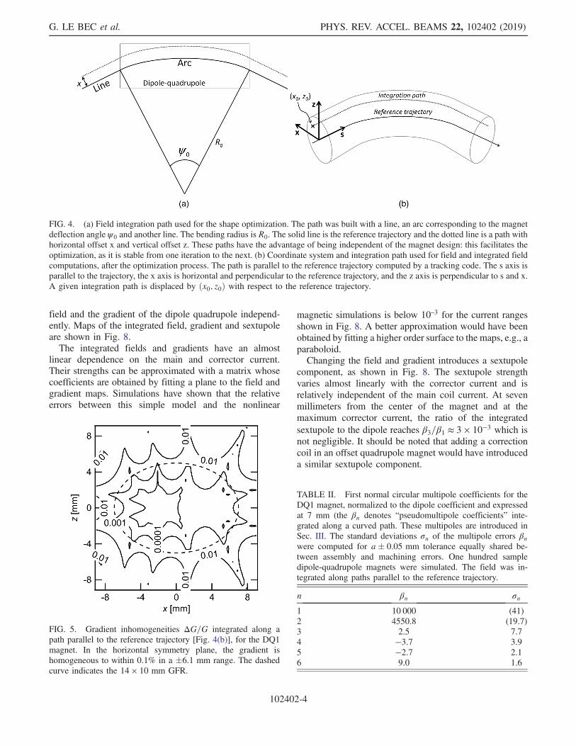
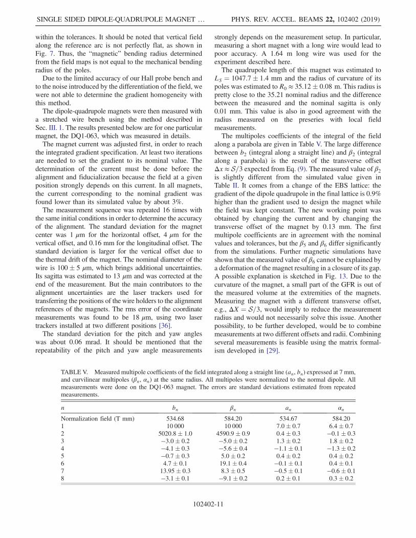
DQ1 geometry, is shown in Fig. 5. The field was integratedalong paths parallel to the reference electron trajectories[Fig. 4(b)], then differentiated to get the relative integratedgradient error ΔG=G. The inhomogeneities appear to be 1order of magnitude below the specifications within thegood field region. The elliptical shape of the good fieldregion is visible on the plot. The first six circular multipolecoefficients are given in Table II.Figure 6 shows the vertical field of the magnet in its

central plane. This field is similar to the field of aquadrupole magnet for x < 15 mm. At higher values ofx (i.e., on the outer part of the ring) the field is close to zero.The field and gradient along the reference axis are

plotted in Fig. 7. It shows that the magnetic lengths forthe dipole and the quadrupole terms are not the same.Using the integrated strength divided by the central strengthas an approximation of the magnetic length, one gets thedipole length L1 ≈ 1054.7 mm and the quadrupole lengthL2 ≈ 1044.0 mm, the iron length being 1028 mm. Indeed, aquadrupole field decreases faster than a dipole field. Theratio between the two magnetic lengths is driven by themagnet bore radius and by the iron length.Two additional air-cooled coils, named correction coils,

were added on the bottom and top auxiliary poles. Thepurpose of the correction coils is to add a knob to tune the

FIG. 3. Sketch of the dipole-quadrupole cross section, show-ing the main parameters of the magnet. The main coil and theauxiliary coils are serially connected. An additional correctioncoil is installed close to the auxiliary pole. The gray ellipsebelow the main pole indicates the approximate position of theelectron beam.

SINGLE SIDED DIPOLE-QUADRUPOLE MAGNET … PHYS. REV. ACCEL. BEAMS 22, 102402 (2019)

102402-3

field and the gradient of the dipole quadrupole independ-ently. Maps of the integrated field, gradient and sextupoleare shown in Fig. 8.The integrated fields and gradients have an almost

linear dependence on the main and corrector current.Their strengths can be approximated with a matrix whosecoefficients are obtained by fitting a plane to the field andgradient maps. Simulations have shown that the relativeerrors between this simple model and the nonlinear

magnetic simulations is below 10–3 for the current rangesshown in Fig. 8. A better approximation would have beenobtained by fitting a higher order surface to the maps, e.g., aparaboloid.Changing the field and gradient introduces a sextupole

component, as shown in Fig. 8. The sextupole strengthvaries almost linearly with the corrector current and isrelatively independent of the main coil current. At sevenmillimeters from the center of the magnet and at themaximum corrector current, the ratio of the integratedsextupole to the dipole reaches β3=β1 ≈ 3 × 10−3 which isnot negligible. It should be noted that adding a correctioncoil in an offset quadrupole magnet would have introduceda similar sextupole component.

FIG. 5. Gradient inhomogeneities ΔG=G integrated along apath parallel to the reference trajectory [Fig. 4(b)], for the DQ1magnet. In the horizontal symmetry plane, the gradient ishomogeneous to within 0.1% in a �6.1 mm range. The dashedcurve indicates the 14 × 10 mm GFR.

FIG. 4. (a) Field integration path used for the shape optimization. The path was built with a line, an arc corresponding to the magnetdeflection angle ψ0 and another line. The bending radius is R0. The solid line is the reference trajectory and the dotted line is a path withhorizontal offset x and vertical offset z. These paths have the advantage of being independent of the magnet design: this facilitates theoptimization, as it is stable from one iteration to the next. (b) Coordinate system and integration path used for field and integrated fieldcomputations, after the optimization process. The path is parallel to the reference trajectory computed by a tracking code. The s axis isparallel to the trajectory, the x axis is horizontal and perpendicular to the reference trajectory, and the z axis is perpendicular to s and x.A given integration path is displaced by ðx0; z0Þ with respect to the reference trajectory.

TABLE II. First normal circular multipole coefficients for theDQ1 magnet, normalized to the dipole coefficient and expressedat 7 mm (the βn denotes “pseudomultipole coefficients” inte-grated along a curved path. These multipoles are introduced inSec. III. The standard deviations σn of the multipole errors βnwere computed for a� 0.05 mm tolerance equally shared be-tween assembly and machining errors. One hundred sampledipole-quadrupole magnets were simulated. The field was in-tegrated along paths parallel to the reference trajectory.

n βn σn

1 10 000 (41)2 4550.8 (19.7)3 2.5 7.74 −3.7 3.95 −2.7 2.16 9.0 1.6

G. LE BEC et al. PHYS. REV. ACCEL. BEAMS 22, 102402 (2019)

102402-4

Random pole displacements and random pole shapeerrors were introduced in the magnetic model in order tosimulate assembly and machining errors. Table II shows thesensitivity for the DQ1, assuming a �0.050 mm mechani-cal tolerance. The relatively high values for these standarddeviations are driven by the small bore radius of a magnet,as we discussed in Ref. [4]. The dipole term has the largeststandard deviation. It translates to a center position uncer-tainty of 64 μm. The standard deviation of the quadrupoleterm gives the gradient error ΔG0=G0 ¼ 4.3 × 10−3 for theDQ1. In practice, these two errors depend on the charac-terization of the magnet: the error on the position of themagnet center is measured and enforced to zero by thefiducialization, and the current is set in order to reachthe nominal gradient. The first significant multipole error isthe sextupole, with a σ3 ¼ 7.7 × 10−4 standard deviation

(normalized to the dipole). Beam dynamics simulationshave shown that, with these levels of higher ordermultipole errors, the impact on the lifetime and dynamic

FIG. 6. Vertical field of the DQ1 dipole-quadrupole magnet inthe longitudinal symmetry plane. The nominal position of thebeam is x ¼ 0.

FIG. 7. Vertical field and gradient along the reference trajec-tory. Notice the longer magnetic length for the dipole field.

FIG. 8. Field and gradient trimming using correction coils:integrated field (top), integrated gradient (middle) and integratedsextupole strength defined as β3=ρ02 (bottom). The strengthswere integrated along paths parallel to the reference trajectory. At7 mm from the center of the magnet and at the maximumcorrector current (2 A), β3=β1 ≈ 0.003.

SINGLE SIDED DIPOLE-QUADRUPOLE MAGNET … PHYS. REV. ACCEL. BEAMS 22, 102402 (2019)

102402-5

aperture is small. In these conditions, assuming 0.05 mmrms alignment errors and taking into account random andsystematic errors on all magnet families, the Touscheklifetime is 22.6� 1.1 hours, the dynamic aperture is 8.5�0.4 millimeters and the injection efficiency is 91.6� 3.2%.These values are acceptable for the EBS.

C. Engineering design

The reduction of the electrical consumption of theaccelerator was one of the goals of the ESRF upgrade.As the magnets are major contributors to the electricalbill, a substantial effort was made to decrease theirconsumption.The power efficiency of the dipole quadrupoles is

improved by a factor of 2 compared to a quadrupole withsimilar gradient and aperture because the DQs are singlesided magnets. The power consumption can be reducedfurther by decreasing the current density (3 A=mm2 for theDQ1). It results in bigger coils, which means more copperand less compact magnets. The DQ1 main coil has 65 turnsand its auxiliary coil has 12 turns. The main coils andauxiliary coils are connected in a series and are watercooled. The magnet power is 1.4 kW at nominal current of85 A. The correction coils are air cooled and their powerconsumption is negligible.Figure 1 shows a design view of the DQ1 magnet. The

yoke is made with seven AISI 1006 low carbon plates. Therepeatability of the yoke and pole assembly is ensuredby the design of the mating surfaces (Fig. 9). Most of themagnet parts are straight, but the pole surfaces are curved,following the reference particle trajectory.The vertical magnetic force applied by the two lower

poles on the two upper poles is 22 kN. This force creates aclosure of the gap by 100 μm. This gap reduction is not abig issue, since the dipole quadrupoles will be powered ina limited range around the nominal current: the deformationcan be compensated by machining the backleg of the yoke100 μm higher than its nominal dimension height.Due to the absence of yoke on one side, the DQs are

less rigid than standard quadrupoles. It would have beenpossible to improve the rigidity by installing nonmagneticstrengthening parts on the open side of the magnet, at thecost of a reduction of the side access to the magnet gap.Another solution would be to increase the thickness of theyoke. The first vibration mode of the DQ1 was found at107 Hz, which was considered to be high enough.

III. MAGNETIC MEASUREMENTS

A. Stretched wire measurementsof the integrated field

Flux meters are often used to map the integrated field ofaccelerator magnets. Rotating coils have been used fordecades and are considered as the reference tools formultipole magnets [25]. Stretched-wire systems, initially

designed for alignment [26,27] and insertion devicesmeasurements [28], can now compete with rotating coilsfor multipole field mapping [29].Unfortunately, none of these solutions are satisfactory

for measuring curved magnets. In a dipole magnet, thefield integral along a straight line has no significancein terms of beam dynamics—even if it may be used forfield quality control, by comparison with simulations.Curved coils have been built by other groups [30]. Suchcoils are well adapted to measure the strength of adipole field. In the case a coil is linearly displacedwithin a field gradient, the accuracy of the measurementis limited [29]. Another possibility is to measure fieldmultipoles at different locations with a rotating coilshorter than the magnet and moved along the referenceaxis of the magnet [31].We developed another method which combines a sim-

plified model of the magnetic field and stretched-wiremeasurements. In the first instance, let us assume that themagnetic field is a pure dipole-quadrupole field within astraight magnetic length LS1 for the dipole and LS2 for thequadrupole and is zero elsewhere (Fig. 10), and that thebending radius of the poles is R0 (Fig. 4). With thissimplified model, the field along the reference trajectoryhas a rectangular shape. Using the notations introducedin the figures, the vertical component of the field can bewritten as

FIG. 9. Yoke of the DQ1 magnet. The yoke is an assembly ofseven parts machined in low carbon plates. The bold solid linesindicate the mating surfaces used for positioning the top of themagnet. The bold dotted lines indicate the mating surface usedfor positioning the auxiliary poles which must be removed forinserting the coils.

G. LE BEC et al. PHYS. REV. ACCEL. BEAMS 22, 102402 (2019)

102402-6

BZðx; yÞ ≈ Bþ G

�x − X0 þ θyþ ðy − ΔyÞ2

2R0

�; ð4Þ

where the quadratic term approximates the curvature of themagnet with a parabola and θ is the angle between themagnet axis and the wire axis. The integral along the wirecan be computed analytically. Assuming θ small and

neglecting the terms in θ2 when integrating along themagnet axis instead of the wire axis [i.e., dy0 ¼cos θ dy ≈ ð1 − θ2=2Þdy ≈ dy], the integral of the field is

IZðx; θÞ

¼ZL=2−L=2

BZdy0 ≈ZL=2−L=2

BZdy

≈ BLS1 þGZ

LS2=2þΔy

−LS2=2þΔy

�x − X0 þ θyþ ðy − ΔyÞ2

2R0

�dy

≈ BLS1 þGLS2

�LS2

2

24R0

þ x − X0 þ θΔy�: ð5Þ

A second integration gives

JZðx; θÞ ≈ZL=2−L=2

Zv−L=2

BZdydv

≈ BLS1ðL=2 − ΔyÞ þ GLS2

�L2

�x − X0 þ

LS22

24R0

�

− Δy2

�LS2

2

12R0

− θLþ 2x − 2X0

�

− θ

�LS2

2

12þ Δy2

��: ð6Þ

Moving the two extremities of the wire in the samedirection gives the IX;Z integrals, while moving only oneextremity of the wire gives the second integrals JX;Z [28].The field integral and second field integral measurementmethods are sketched in Fig. 10.Let us first measure the field integral at two wire

positions IZ01 ¼ IZðΔX; θ0Þ and IZ02 ¼ IZð−ΔX; θ0Þ; theaxis of the magnet being determined by the unknownposition X0 and angle θ0. The difference of these twointegrals simplifies to IZ01 − IZ02 ¼ 2GLS 2Δx, so theintegrated gradient is

GLS2 ¼IZ01 − IZ02

2Δx: ð7Þ

The transverse position and angle and the above fieldintegrals satisfy

X0 ¼1

GLS2

�BLS1 − IZ01 þ IZ02

2

�þ LS2

2

24R0

þ θ0Δy: ð8Þ

The sagitta of the trajectory is S ≈ LS2=8R0 and in the

case ðθ0;ΔyÞ ¼ 0 this equation simplifies to

FIG. 10. Top: Simplified field model used for the measurementof the dipole-quadrupole magnets. The field is assumed to benonzero over a length LS and the radius of curvature of themagnet poles is R0. The magnet is measured using a stretchedwire of length L. The longitudinal distance between the magnetand the wire center is Δy. The dashed line represents the wire.The magnet frame is ðx; yÞ and the wire frame is ðx0; y0Þ. Middle:If the two extremities of the wire are moved in the same direction,the induced voltage e is proportional to the integral of the fieldIðX0; θ0Þ. If only one extremity of the wire is moved, the inducedvoltage varies with the second integral of the field JðX0; θ0Þ.Bottom: In the “pseudocurvilinear multipole” approximationdeveloped in this paper, the field of the dipole-quadrupole magnetis modeled as a succession of parallel slices. In each slice, thefield is approximated by an analytic function, i.e., a Taylor series.The multipole coefficients are assumed to be the same for allslices.

SINGLE SIDED DIPOLE-QUADRUPOLE MAGNET … PHYS. REV. ACCEL. BEAMS 22, 102402 (2019)

102402-7

X0 ¼1

GLS2

�BLS1 − IZ01 þ IZ02

2

�þ S

3: ð9Þ

This result was first demonstrated by Jain [32]. Then,let us measure the field integrals at X0 and θ0 � Δθ∶IZ11 ¼ IZðX0; θ0 þ ΔθÞ, JZ11 ¼ JZðX0; θ0 þ ΔθÞ, IZ12 ¼IZðX0; θ0 − ΔθÞ and JZ12 ¼ JZðX0; θ0 − ΔθÞ. Combiningthe first field integrals gives the longitudinal position ofthe magnet,

Δy ¼ IZ11 − IZ122GLS 2Δθ

; ð10Þ

while the straight magnetic length is deduced from thedifferences of the second field integral:

LS 2 ¼ffiffiffiffiffiffiffiffiffiffiffiffiffiffiffiffiffiffiffiffiffiffiffiffiffiffiffiffiffiffiffiffiffiffiffiffiffiffiffiffiffiffiffiffiffiffiffiffiffiffiffiffiffiffiffiffiffiffiffiffiffiffiffiffiffiffiffiffiffiffiffiffiffiffiffiffiffiffi

6

GLS 2ΔθðJZ12 − JZ11Þ þ 6ΔyðL − 2ΔyÞ

s: ð11Þ

The length of the curved reference path can be deducedusing the following series expansion:

LC2 ≈ LS2

�1þ LS2

2

24R02

�: ð12Þ

The wire yaw angle is computed from a combination ofthe first and second field integrals:

θ0 ¼6L

GLS23

�ðIZ11 þ IZ12ÞðL=2 − ΔyÞ − ðJZ11 þ JZ12Þ

�:

ð13Þ

The position X0 is then obtained by inserting in Eq. (8)the values θ0 obtained from Eq. (13) and Δy obtainedfrom Eq. (10).All of the above parameters were obtained with an a priori

value for R0. Let us now compare the second integrals JZ11and JZ12, obtained on a magnet whose curvature radius isR0 þ ΔR0, to the a priori values JZ110 and JZ120 computedassuming a radius R0. From a series expansion of Eq. (6),we get

ΔR0 ≈24R0

2

GLS23ðL − 2ΔyÞ ðJZ110 þ JZ120 − JZ11 − JZ12Þ:

ð14Þ

The radius of curvature can thus be obtained from thedifference between the measured second field integrals andtheir value assuming R0.One should note that the above method can be used for

quadrupole alignment, by setting B ¼ 0 and R0 → ∞. Thevertical position and the pitch angle of the magnetic axisare obtained in this particular case.

We have shown that a few first and second field integralmeasurements fully determine the magnet alignment,including its longitudinal position and the pitch and yawangles. The same measurements give most of the param-eters of the model: the field gradient, the quadrupolemagnetic length and the radius of curvature of the poles.The dipole magnetic length, not determined here, can betaken as being equal to the quadrupole length as a firstapproximation.Let us now assume that the wire is aligned on the magnet

axis. In the case where the magnetic field is not a puredipole quadrupole but contains higher order multipoles, thefield integral can be approximated by

IZ þ iIX ¼Z

ðBZ þ iBxÞdl ¼Xn>0

ðbn þ ianÞ�ur0

�n−1

≈Xn>0

βn þ iαnLSr0n−1

ZLS=2

−LS=2

�uþ y2

2R0

�n−1

dy; ð15Þ

where u ¼ xþ iz is the complex variable, an and bn arethe multipole coefficients of the integrated field (see theAppendix) and βn and αn are “pseudocurvilinear multi-pole” coefficients integrated along the curved trajectory.The arc is approximated by the parabola x ¼ y2=ð2R0Þ.We neglect here the fringe field terms. The effect of these

terms will be discussed in Sec. IV.Applying the binomial formula to Eq. (15) and integrat-

ing leads to

IZ þ iIX ≈ −Xn>0

Xn−1k¼0

ðβn þ iαnÞ�n − 1

k

�

×

�LS

2

8R0r0

�n−1−k 1

1þ 2ðk − nÞ�ur0

�k

≈Xn>0

ðbn þ ianÞ�ur0

�n−1

: ð16Þ

TheN first terms of this equation can be written in matrixform

0BB@

b1 þ ia1

..

.

bN þ iaN

1CCA ¼

0BB@

A11 � � � A1N

..

. . .. ..

.

0 � � � ANN

1CCA0BB@

β1 þ iα1

..

.

βN þ iαN

1CCA;

ð17Þ

with

G. LE BEC et al. PHYS. REV. ACCEL. BEAMS 22, 102402 (2019)

102402-8

Amn ¼ðn − 1Þ!

ðm − 1Þ!ðn −mÞ!½1 − 2ðm − nÞ��

LS2

8R0r0

�n−m

;

n ≥ m: ð18Þ

The an and bn can be measured with a stretched wire[29], as well as the magnetic length LS and on the radiusof curvature R0 which appear in the matrix A. Thepseudocurvilinear multipole coefficients βn and αn canthus be obtained from the (pseudo)inverse Aþ of A:0

BB@β1 þ iα1

..

.

βN þ iαN

1CCA ¼ Aþ

0BB@

b1 þ ia1

..

.

bN þ iaN

1CCA: ð19Þ

These results are valid in the case where the magnet islongitudinally centered on the wire, i.e., Δy ¼ 0. This isusually not true in practice: the term y2 in Eq. (15) shouldbe replaced by ðy − ΔyÞ2. Inserting the longitudinal posi-tion in the equations lead to a more complex expression forthe matrix coefficients:

Amn ¼ðn − 1Þ!½ðLS

2− ΔyÞ2ðn−mÞþ1 þ ðLS

2þ ΔyÞ2ðn−mÞþ1�

ðm − 1Þ!ðn −mÞ!½1 − 2ðm − nÞ�LSð2R0r0Þn−m;

n ≥ m; ð20Þ

which simplifies to Eq. (18) if Δy ¼ 0.One should note that the presence of binomial coef-

ficients in the Amn makes the inversion ofA unstable if N istoo large. For all n > 20, we set an and bn to zero to avoidinversion issues.The coefficients obtained with Eq. (19) can easily be

converted to pseudoelliptic multipole coefficients Ek usingthe matrix notations introduced in the Appendix:

0BBB@

..

.

Ek

..

.

1CCCA ¼ ME

−1MCAþ

0BBB@

..

.

bk þ iak

..

.

1CCCA: ð21Þ

The methods described above were first tested with a 3Dmodel of the DQ1 dipole quadrupole. Pseudomultipoles ofthe integrated field were given in Table II. AssumingR0 ¼ 35.20 m, enforcing BLS 1 ¼ 0.5844 Tm and usingEq. (5) to (14) lead to the values given in Table III. InSec. II B, the quadrupole magnetic length, defined as theintegrated gradient divided by the central gradient, wasfound equal to 1044 mm, which is almost the same value asin Table III.A 35.255 m bending radius was estimated from the

integrals along straight lines. It is close to the nominalradius: the relative difference between the two radiuses isabout 0.15%. However, this requires further verification:

any method giving a small ΔR0 would lead to a smalldifference between the nominal radius and the estimatedone. To check this, the assumed value of R0 in Eq. (5) toEq. (14) was modified and the bending radius wasestimated. The results plotted in Fig. 11 shows that themethod remains accurate even if the assumed value of R0

is wrong.Table IV shows the pseudomultipole coefficients com-

puted with Eq. (19) and allow a comparison to thepseudomultipoles integrated along curves parallel to thereference trajectory and to the pseudomultipoles integrated

TABLE III. Determination of the magnet properties fromintegrals of the field along straight lines. The field integralsIZ01, IZ02, IZ11, IZ12 and the second field integrals JZ11 and JZ12were computed with a 3D model of the DQ1 magnet, using theRadia software. The JZ110 and JZ120 integrals were computedusing Eq. (6), the integrated gradient was obtained from Eq. (7),the quadrupole magnetic length was computed from Eq. (11) andthe bending radius was determined using Eq. (14).

IZ01 0.630 45 T mIZ02 0.440 49 T mIZ11 0.535 44 T mIZ12 0.535 44 T mJZ11 0.413 10 Tm2

JZ12 0.390 09 Tm2

JZ11 0 0.413 10 Tm2

JZ12 0 0.390 10 Tm2

GLS2 −37.991 TLS2 1.0439 mR0 þ ΔR0 35.255 m

FIG. 11. Bending radius estimated from the field integralmethod versus assumed bending radius. If the assumed bendingradius is wrong by 5 m, the error in the bending radius estimationis about 0.7 m. A 1 m error in the assumed bending radius gives a3 cm error in the estimation (from 3D simulations with Radia).

SINGLE SIDED DIPOLE-QUADRUPOLE MAGNET … PHYS. REV. ACCEL. BEAMS 22, 102402 (2019)

102402-9

along parabolas. The agreement between the differentmethods is 2 × 10−4 or better for all coefficients.The reference trajectory is well approximated by a

parabola in the interior of the magnet but this is not thecase in the fringe field region. However, Table IV dem-onstrates that integrals of the field along parabolas are goodapproximations of the field integrals along the referencetrajectories.

B. Magnetic measurement benches

A Hall probe bench designed at the ESRF for undulatormeasurements [33] was used for measuring locally themagnetic field. The Hall sensors were calibrated versus anuclear magnetic resonance probe in a dipole magnet.Then, the dipole-quadrupole magnets were measured

with stretched wire benches. These benches are madewith Newport ILS-100CC and IMS-100V linear stages,driven by a Newport XPS motion controller. The stageswere calibrated with an interferometer and their accuracyis in the range of 1 μm. The voltage induced on the wirewas measured with a Keitley 2182 voltmeter. A 0.1 mmdiameter Ti-6Al-4V wire was used. Please refer to Ref. [34]for a more detailed presentation of the ESRF stretched wirebenches.The following measurement sequence was implemented

on the measurement bench: (i) measurement of the fieldintegrals and the second field integrals IZ01, IZ02, IZ11, IZ12,IX11, IX12, JZ11, JZ12, JX11 and JX12 and determination ofthe gradient, longitudinal position, yaw and pitch angle,magnetic length and curvature, (ii) measurement of theintegrated field at 128 points on a circle with 9 mm

diameter, i.e., at the maximum radius compatible withthe geometry of the curved poles. All the measurementsequences and the analysis routines are part of the opensource software SW Lab currently developed at theESRF [35].

C. Results

Two kinds of measurements were performed on the DQmagnets: local measurements with a Hall probe bench, andintegral measurements with a stretched wire bench.The field and gradient are shown in Fig. 12. These

measurements were used to determine the dipole lengthL1MEAS ¼ 1056 mm (simulated value 1054.7 mm) and thequadrupole length L2MEAS ¼ 1045 mm (simulated value1044.0 mm). The magnetic lengths were defined as theintegral of the field divided by its central value.The bending radius of the poles was also determined

from the local measurements, assuming that the verticalfield BZ is homogeneous on the trajectory and excludingthe extremities of the magnet. The best fitted value of thecurvature radius is 35.06 m, which is close to the 35.20 mspecified mechanical radius. Considering the deflectionangle of the DQ1, the error on the sagitta of the magnet is(35.20–35.06) ð1 − cos 0.0292=2Þ ≈ 15 μm, which is well

FIG. 12. Top: Magnetic field of the DQ1 preseries magnetDQ1-002, measured with a Hall probe bench. Step size:1 mm. Bottom: Field gradient obtained by differentiating themagnetic field.

TABLE IV. Simulated pseudomultipoles of the integrated fieldcomputed with different methods. (Trajectory): The field wasintegrated along curves parallel to the reference trajectory.(Parabola): The field was integrated along parabolas with35.255 m curvature radius. (Straight to parabola): The fieldwas integrated along straight lines, then Eq. (19) was used inorder to compute pseudomultipoles integrated along a parabola.The horizontal and the vertical field components were sampled oncircles centered on the parabola and with symmetry axis parallelto the magnet axis.

Trajectory Parabola Straight to parabola

Normalizationfield (T mm)

584.38 585.72 585.72

n βn βn βn1 10 000 10 000 10 0002 −4550.8 −4548.0 −4548.53 2.5 2.1 4.14 3.7 3.8 3.75 −2.7 −2.6 −2.96 −9.0 −9.3 −9.67 2.9 2.8 1.98 9.5 10.1 11.0

G. LE BEC et al. PHYS. REV. ACCEL. BEAMS 22, 102402 (2019)

102402-10

within the tolerances. It should be noted that vertical fieldalong the reference arc is not perfectly flat, as shown inFig. 7. Thus, the “magnetic” bending radius determinedfrom the field maps is not equal to the mechanical bendingradius of the poles.Due to the limited accuracy of our Hall probe bench and

to the noise introduced by the differentiation of the field, wewere not able to determine the gradient homogeneity withthis method.The dipole-quadrupole magnets were then measured with

a stretched wire bench using the method described inSec. III. 1. The results presented below are for one particularmagnet, the DQ1-063, which was measured in details.The magnet current was adjusted first, in order to reach

the integrated gradient specification. At least two iterationsare needed to set the gradient to its nominal value. Thedetermination of the current must be done before thealignment and fiducialization because the field at a givenposition strongly depends on this current. In all magnets,the current corresponding to the nominal gradient wasfound lower than its simulated value by about 3%.The measurement sequence was repeated 16 times with

the same initial conditions in order to determine the accuracyof the alignment. The standard deviation for the magnetcenter was 1 μm for the horizontal offset, 4 μm for thevertical offset, and 0.16 mm for the longitudinal offset. Thestandard deviation is larger for the vertical offset due tothe thermal drift of the magnet. The nominal diameter of thewire is 100� 5 μm, which brings additional uncertainties.Its sagitta was estimated to 13 μm and was corrected at theend of the measurement. But the main contributors to thealignment uncertainties are the laser trackers used fortransferring the positions of the wire holders to the alignmentreferences of the magnets. The rms error of the coordinatemeasurements was found to be 18 μm, using two lasertrackers installed at two different positions [36].The standard deviation for the pitch and yaw angles

was about 0.06 mrad. It should be mentioned that therepeatability of the pitch and yaw angle measurements

strongly depends on the measurement setup. In particular,measuring a short magnet with a long wire would lead topoor accuracy. A 1.64 m long wire was used for theexperiment described here.The quadrupole length of this magnet was estimated to

LS ¼ 1047.7� 1.4 mm and the radius of curvature of itspoles was estimated to R0 ≈ 35.12� 0.08 m. This radius ispretty close to the 35.21 nominal radius and the differencebetween the measured and the nominal sagitta is only0.01 mm. This value is also in good agreement with theradius measured on the preseries with local fieldmeasurements.The multipoles coefficients of the integral of the field

along a parabola are given in Table V. The large differencebetween b2 (integral along a straight line) and β2 (integralalong a parabola) is the result of the transverse offsetΔx ≈ S=3 expected from Eq. (9). The measured value of β2is slightly different from the simulated value given inTable II. It comes from a change of the EBS lattice: thegradient of the dipole quadrupole in the final lattice is 0.9%higher than the gradient used to design the magnet whilethe field was kept constant. The new working point wasobtained by changing the current and by changing thetransverse offset of the magnet by 0.13 mm. The firstmultipole coefficients are in agreement with the nominalvalues and tolerances, but the β5 and β6 differ significantlyfrom the simulations. Further magnetic simulations haveshown that the measured value of β6 cannot be explained bya deformation of the magnet resulting in a closure of its gap.A possible explanation is sketched in Fig. 13. Due to thecurvature of the magnet, a small part of the GFR is out ofthe measured volume at the extremities of the magnets.Measuring the magnet with a different transverse offset,e.g., ΔX ¼ S=3, would imply to reduce the measurementradius and would not necessarily solve this issue. Anotherpossibility, to be further developed, would be to combinemeasurements at two different offsets and radii. Combiningseveral measurements is feasible using the matrix formal-ism developed in [29].

TABLE V. Measured multipole coefficients of the field integrated along a straight line (an, bn) expressed at 7 mm,and curvilinear multipoles (βn, αn) at the same radius. All multipoles were normalized to the normal dipole. Allmeasurements were done on the DQ1-063 magnet. The errors are standard deviations estimated from repeatedmeasurements.

n bn βn an αn

Normalization field (T mm) 534.68 584.20 534.67 584.201 10 000 10 000 7.0� 0.7 6.4� 0.72 5020.8� 1.0 4590.9� 0.9 0.4� 0.3 −0.1� 0.33 −3.0� 0.2 −5.0� 0.2 1.3� 0.2 1.8� 0.24 −4.1� 0.3 −5.6� 0.4 −1.1� 0.1 −1.3� 0.25 −0.7� 0.3 5.0� 0.2 0.4� 0.2 0.4� 0.26 4.7� 0.1 19.1� 0.4 −0.1� 0.1 0.4� 0.17 13.95� 0.3 8.3� 0.5 −0.5� 0.1 −0.6� 0.18 −3.1� 0.1 −9.1� 0.2 0.2� 0.1 0.3� 0.2

SINGLE SIDED DIPOLE-QUADRUPOLE MAGNET … PHYS. REV. ACCEL. BEAMS 22, 102402 (2019)

102402-11

The integrated gradient and its homogeneity can becomputed from the multipoles. Homogeneity contours areshown in Fig. 14. The normalized gradient error ΔG=G iswell below the 1% specification. It is under 0.1% within a�5.3 mm range in the horizontal direction. (Magneticsimulation gave a 0.1% homogeneity within a �6.1 mmrange, see Fig. 5.)

IV. EFFECT OF THE MAGNET’S CURVATURE

In the above discussion, the field of the magnet wasapproximated by a set of slices. The field in each slice wasassumed to be an analytic function. For straight magnets thisapproximation gives the correct integrals of the field, even ifit hides the fringe field effect. (We discussed some effects ofthe fringe field of quadrupole magnets in Ref. [4].)In this discussion, we will focus on the integral of the

fields along the reference trajectory of the electrons[Fig. 4(b)]. The field integral along a curved path differsfrom an analytic function. Stated differently, reconstructingthe field from Fourier coefficients estimated on theboundary of a given region would lead to errors insidethis region. For a given magnet model, these errors canbe simulated easily. Complex field integrals Ik ¼

R ðBz þiBxÞds were computed at uk ¼ xk þ izk ¼ ρ0ExpðiθkÞ,where ρ0 is the radius of the good field region, θk ¼2πk=K and 0 ≤ k < K. The path length depends on uk andthe reference trajectory corresponds to u ¼ 0. In the casethese field integrals would be an analytic function of u, theseries coefficients would be obtained from the Fouriertransform of the signal I ¼ ðI1;…; IKÞ, as is usually donefor multipole analysis. Let us denote an and bn the seriescoefficients obtained from the Fourier transform of I. Then,a field integral error can be estimated at each point ðx; zÞinside the good field region:

εðx; zÞ ¼jIðx; zÞ −P

n≥1ðbn þ ianÞðxþizρ0

Þn−1jmax jIðx; zÞj : ð22Þ

This error is shown in Fig. 15. It demonstrates that withinthe good field region the integral of the field along paths

FIG. 14. Homogeneity contours of the magnetic field gradientintegrated along a straight line and along a parabola whoseminimal radius of curvature is equal to the measured bendingradius of the magnet. The dotted line in black indicates the 14 mmx 10 mm good field region. In the horizontal plane, the gradientintegrated along the parabola has a homogeneity better than 0.1%in a �5.3 mm range.

FIG. 15. Contour plot of the error 104εðx; zÞ defined inEq. (22). This error is the normalized difference between theintegral of the field along a path parallel to the referencetrajectory, and an analytic function whose series coefficientswere evaluated from the values of the integrated field on a 7 mmradius circle. The higher values of the error, on the boundary, aredue to the truncation of the series to its ten first terms.

FIG. 13. Cut view of a DQ1 from its center, showing thetrajectory of the wire and the GFR in the middle and at theextremities. The wire rotation axis was tangent to the referencetrajectory in the middle of the magnet. At the magnet extremities,a part of the GFR is out of the measurement radius. This may be acause of the discrepancies between simulations and measure-ments for the higher order harmonics.

G. LE BEC et al. PHYS. REV. ACCEL. BEAMS 22, 102402 (2019)

102402-12

parallel to the trajectory can be approximated with a relativeerror below 10−4 with a Fourier expansion.Solutions of the Laplace equation in curvilinear coor-

dinates, i.e., curvilinear multipoles, have been studied byothers. Cylindrical multipoles were first proposed byMcMillan [37], rediscovered independently by Mane[38] and studied in more details by Zolkin [39]. Toroidalfield multipoles were studied by other authors. Schnizeret al. introduced a local toroidal coordinate system andshown the curvature results in distortions of the standardfield multipoles [24,40]. Wolski and Herrod have recentlypublished an expression of the potential in toroidal coor-dinates [41]. We implemented a similar toroidal multipoleexpansion and we computed the error between the fieldintegral and a sum of toroidal multipoles. For the magnetwe investigated, the relative error was again in the 10−4range. As the toroidal multipoles are a solution of theLaplace equations in this geometry, the field at a givenpoint should be equal to the toroidal multipole series at thesame point. This indicates that the accuracy of the compu-tations is about 10−4.

V. CONCLUSION

Off-axis quadrupoles are suitable to achieve the speci-fications of the combined dipole quadrupoles to be inte-grated in the new generation of storage ring based lightsources. These magnets can be asymmetric in order toreduce their electrical power consumption. Such magnetswere designed and constructed for the EBS. The shapes ofthe magnets were optimized in order to obtain a goodgradient homogeneity within an elliptic good field region.The magnets are single sided and produce almost no fieldon their outer side. Correction coils were installed in orderto tune the field and the gradient independently.Stretched wire magnetic measurement methods were

developed for the magnet alignment and for measuring itsmain parameters, i.e., magnetic length, gradient, polebending radius and pseudomultipole coefficients. Theaccuracy of these methods was demonstrated with 3Dsimulations. The parameters measured on one of the dipole-quadrupole magnet series were presented. The alignmentaccuracy was very good, the fiducialization errors beingdominated by laser tracker uncertainties. The multipolecoefficients were in good agreement with the simulationresults and tolerances up to the octupole, but the decapoleand dodecapole are significantly higher than their simulatedvalue. These discrepancies may be explained by theimperfect matching of the volume measured by the wireand the GFR volume. Combining two or more measure-ments performed at different offsets and radii would allowovercoming this issue but would need further develop-ments. It should be noted that the stretched wire methodsdeveloped in the paper may be adapted to rotating coilmeasurements.

If the field integral is evaluated on a curved path ratherthan on a straight line, it is not an analytic function.However, we have shown that given the large radius ofcurvature and the small radius of the good field region forthe magnets described here, the relative error between theintegral of the field and its analytic approximation is notlarger than 10–4.

ACKNOWLEDGMENTS

The authors would like to thank Dr. C. Benabderrahmanewho followed up the production of the DQ series magnets,and the magnet company Tesla Engineering Ltd., UK, whoproduced all of the dipole quadrupoles for the EBS.

APPENDIX

1. Standard multipoles and elliptic multipolesfor straight magnets

The field of multipole accelerator magnets is oftenexpressed as a multipole series: the magnetic field isdescribed with a small number of coefficients, makingits representation easier. The most common multipoles arethe 2D “straight” multipoles obtained by integration of thefield along a line.Within the aperture of a multipole magnet, the Maxwell

equations reduce to∇ · B ¼ 0 and∇ ×B ¼ 0. The integralof a magnetic field along a straight line is a 2D field, forwhich the Maxwell equations are equivalent to the Cauchy-Riemann equations. The complex field B ¼ BZ þ iBX,where BZ and BX are the vertical and horizontal compo-nents of the integral of the field along a straight line, can beexpressed as the Taylor series

B ¼X∞n¼1

ðbn þ ianÞ�uρ0

�n−1

;

where u ¼ xþ iz is the complex function, bn and an arethe normal and skew 2n-pole coefficients and ρ0 is thereference radius.The apertures of dipole magnets are often noncircular.

Elliptic multipoles have been introduced by Schnizer et al.[23,24] for describing the dipole fields on noncircularaperture. The elliptic coordinates are defined as x ¼e cosh η cosψ and z ¼ e sinh η sinψ , where e is the eccen-tricity, 0 ≤ η < ∞ and −π ≤ ψ < π. Cartesian coordinatesare transformed to elliptic coordinates by the conformalmap

w ¼ ηþ iψ ¼ Arccoshðu=eÞ:

Inserting this in standard multipole series and usingMoivre’s formula and the binomial theorem, then rearrang-ing the terms and introducing new notations leads to

SINGLE SIDED DIPOLE-QUADRUPOLE MAGNET … PHYS. REV. ACCEL. BEAMS 22, 102402 (2019)

102402-13

B ¼ E0

2þX∞n¼1

EncoshðnwÞcoshðnη0Þ

: ðA1Þ

The En’s are the elliptic multipole coefficients while η0 isa normalization factor.If the summation in Eq. (A1) is truncated to its first

terms, the field at a given set of points can be expressed inmatrix form:

B ¼ MEE; ðA2Þ

where Bi ¼ BðwiÞ, the Ej’s are the complex elliptic multi-pole coefficients, 1 ≤ i ≤ M, 1 ≤ j ≤ N and

MEij ¼� 1

2for j ¼ 1

ℬ cosh½ðj−1Þwi�cosh½ðj−1Þη0� for j > 1.

This multipole expansion has been used for optimizingthe field on an elliptical good field region.Similarly, the field in polar coordinates writes B ¼

MCC, where theCj’s are the complexmultipole coefficientsand MCij ¼ ðui=ρ0Þj−1. One can choose the points i suchthat the matrix MC is invertible. In such a case, the ellipticmultipoles transform to the circular ones according to

C ¼ MC−1MEE: ðA3Þ

This yields kCkF ≤ kMC−1MEkFkEkF where kAkF is

the Frobenius norm of A. The norm K ¼ kMC−1MEkF

depends only on the positions at which the field iscomputed, i.e., on the good field region, so the minimiza-tion of the elliptic multipole errors kεEk ¼ kE −ETARGETkfor a given good field region yields to small circularmultipole errors: kεCk ≤ KkεEk.

[1] L. Farvacque, N. Carmignani, J. Chavanne, A. Franchi, G.Le Bec, S. Liuzzo, B. Nash, T. Perron, P. Raimondi, A low-emittance lattice for the ESRF, in Proceedings of the 4thInternational Particle Accelerator Conference, IPAC-2013, Shanghai, China, 2013 (JACoW, Shanghai, China,2013), pp. 79–81.

[2] J. C. Biasci, J. F. Bouteille, N. Carmignani, J. Chavanne, D.Coulon, Y. Dabin, F. Ewald, L. Farvacque, L. Goirand, M.Hahn et al., A low-emittance lattice for the ESRF,Synchrotron Radiat. News 27, 8 (2014).

[3] G. Le Bec, J. Chavanne, F. Villar, C. Benabderrahmane, S.Liuzzo, J.-F. Bouteille, L. Goirand, L. Farvacque, J.-C.Biasci, and P. Raimondi, Magnets for the ESRF diffractionlimited light source project, IEEE Trans. Appl. Supercond.26, 1 (2016).

[4] G. Le Bec, J. Chavanne, C. Benabderrahmane, L. Farvacque,L. Goirand, S. Liuzzo, P. Raimondi, and F. Villar, Highgradient quadrupoles for low emittance storage rings, Phys.Rev. Accel. Beams 19, 052401 (2016).

[5] J. Chavanne and G. Le Bec, Prospects for the use ofpermanent magnets in future accelerator facilities, inProceeding of the International Particle AcceleratorConference 14 (IPAC14), Dresden, Germany (JACoW,Dresden, Germany, 2014), pp. 968–973.

[6] E. D. Courant, M. S. Livingston, and H. S. Snyder, Thestrong-focusing synchrotron—A new high energy accel-erator, Phys. Rev. 88, 1190 (1952).

[7] Y. Chen, D. E. Kim, W. Kang, F. S. Chen, M. Yang, Z.Zhang, B. G. Yin, and J. X. Zhou, Designs and measure-ments of gradient dipole magnets for the upgrade ofPohang Light Source, Nucl. Instrum. Methods Phys.Res., Sect. A 682, 85 (2012).

[8] D. Einfeld, M. Melgoune, G. Beneditti, M. De Lima, J.Marcos, M. Munoz, M. Pont, Modelling of gradientbending magnets for the beam dynamics studies at ALBA,in Proceedings of the 22nd Particle AcceleratorConference, PAC-2007, Albuquerque, NM (IEEE, NewYork, 2007), pp. 1076–1078.

[9] L. Dallin, I. Blomqvist, D. Lowe, J. Swirksy, J. Campmany,F. Goldie, J. Coughlin, Gradient dipole magnets for theCanadian Light Source, in Proceedings of the 8th EuropeanParticle Accelerator Conference, Paris, 2002 (EPS-IGAand CERN, Geneva, 2002).

[10] J. A. Eriksson, A. Andersson, M. Johansson, D. Kumbaro,S. C. Leemann, C. Lenngren, P. Lilja, F. Lindau, L.-J.Lindgren, L. Malgren et al., The MAX IV synchrotronlight source, in Proceedings of the 2nd InternationalParticle Accelerator Conference, San Sebastián, Spain(EPS-AG, Spain, 2011), pp. 3026–3028.

[11] M. Johansson, B. Anderberg, and L. J. Lindgren, Magnetdesign for a low-emittance storage ring, J. SynchrotronRadiat. 21, 884 (2014).

[12] M. Yoon, J. Corbett, M. Cornacchia, J. Tanabe, andA. Terebilo, Analysis of a storage ring combined-function magnet: Trajectory calculation and alignmentprocedure, Nucl. Instrum. Methods Phys. Res., Sect. A523, 9 (2004).

[13] M. Sjöström, E. Wallen, M. Eriksson, and L. J. Lindgren,The MAX III storage ring, Nucl. Instrum. Methods Phys.Res., Sect. A 601, 229 (2009).

[14] M. Borland, V. Sajaev, Y. Sun, and A. Xiao, Hybrid seven-bend-achromat lattice for the advanced photon source up-grade, in Proceeding of the International Particle Acceler-ator Conference 15 (IPAC15), Richmond, USA, 2015,pp. 1776–1779.

[15] C. Steier, J. Byrd, H. Nishimura, D. Robin, S. De Santis, F.Sannibale, C. Sun, M. Venturini, W. Wan, Physics designprogress towards a diffraction limited upgrade of the ALS,in Proceeding of the International Particle AcceleratorConference 16 (IPAC16), Busan, Korea, 2016, pp. 2956–2958.

[16] H. Tanaka, T. Ishikawa, S. Goto, S. Takano, T. Watanabe,and M. Yabashi, SPring-8 upgrade project, in Proceedingof the International Particle Accelerator Conference 16(IPAC16), Busan, Korea, 2016, pp. 2867–2870.

[17] E. Karantzoulis, The diffraction limited light sourceELETTRA 2.0, in Proceeding of the International ParticleAccelerator Conference 17 (IPAC17), Copenhagen,Denmark, 2017, pp. 2660–2662.

G. LE BEC et al. PHYS. REV. ACCEL. BEAMS 22, 102402 (2019)

102402-14

[18] B. Parker, N. L. Smirnov, and L. M. Tkachenko, Develop-ment of septum quadrupole prototype for DESYupgradingluminosity, Nucl. Instrum. Methods Phys. Res., Sect. A434, 297 (1999).

[19] P. Elleaume, O. Chubar, and J. Chavanne, Computing 3Dmagnetic fields from insertion devices, in Proceedings ofthe Particle Accelerator Conference, Vancouver, BC,Canada, 1997 (IEEE, New York, 1997), pp. 3509–3511.

[20] O. Chubar and P. Elleaume, Accurate and efficient com-putation of synchrotron radiation in the near field region, inProceedings of the 6th European Particle AcceleratorConference, Stockholm, 1998 (IOP, London, 1998).

[21] G. Le Bec, J. Chavanne, and P. N’gotta, Shape optimiza-tion for the ESRF II magnets, in Proceeding of theInternational Particle Accelerator Conference 14,IPAC14, Dresden, 2014, pp. 1232–1234.

[22] S. Russenschuck, Field Computation for AcceleratorMagnets (Wiley-VCH, New York, 2010).

[23] P. Schnizer, B. Schnizer, P. Akishin, and E. Fischer, Theoryand application of plane elliptic multipoles for staticmagnetic fields, Nucl. Instrum. Methods Phys. Res., Sect.A 607, 505 (2009).

[24] P. Schnizer, B. Schnizer, P. Akishin, and E. Fischer, Planeelliptic or toroidal multipole expansions for static fields.Applications within the gap of straight and curved accel-erator magnets, COMPEL 28, 1044 (2009).

[25] L. Walckiers, The harmonic-coil method, in CERN Accel-erator School: Magnetic measurement and alignment,Montreux, Switzerland, 1992, pp. 138–166.

[26] J. DiMarco and J. Krzywinski, MTF single stretched wiresystem, Fermilab MTF-96-0001, 1996.

[27] J. DiMarco, H. Glass, M. J. Lamm, P. Schlabach, C.Sylvester, J. C. Tompkins, and I. Krzywinski, Field align-ment of quadrupole magnets for the LHC interactionregions, IEEE Trans. Appl. Supercond. 10, 127 (2000).

[28] D. Zangrando and R. P. Walker, A stretched wire systemfor accurate integrated magnetic field measurements in

insertion devices, Nucl. Instrum. Methods Phys. Res., Sect.A 376, 275 (1996).

[29] G. Le Bec, J. Chavanne, and C. Penel, Stretched wiremeasurement of multipole accelerator magnets, Phys. Rev.ST Accel. Beams 15, 022401 (2012).

[30] G. Deferme, Advances in stretched wire systems at CERN,in IMMW19, Hsinchu, Taiwan, 2015.

[31] J. DiMarco, Recent PCB rotating coil developments atFermilab, in IMMW19, Hsinchu, Taiwan, 2015.

[32] A. K. Jain, Magnet alignment challenges for an MBAstorage ring, in DLSR, Lemont, USA, 2014.

[33] J. Chavanne and P. Elleaume, Technology of insertiondevices, in Undulators, Wigglers and their Applications,edited by H. Onuki and P. Elleaume (Taylor & Francis,London, 2003), pp. 148–213.

[34] G. Le Bec, Overview of magnetic measurement activities atthe ESRF, in IMMW20, Didcot, UK, 2017.

[35] SW Lab, https://gitlab.esrf.fr.[36] D. Martin, Alignment of the ESRF Extremely Brilliant

Source (EBS), in IWAA, Chicago, USA, 2018.[37] E. M. McMillan, Multipoles in cylindrical coordinates,

Nucl. Instrum. Methods 127, 471 (1975).[38] S. R. Mane, Solutions of Laplace’s equation in two

dimensions with a curved longitudinal axis, Nucl. Instrum.Methods Phys. Res., Sect. A 321, 365 (1992).

[39] T. Zolkin, Sector magnets or transverse electromagneticfields in cylindrical coordinates, Phys. Rev. Accel. Beams20, 043501 (2017).

[40] P. Schnizer, E. Fischer, and B. Schnizer, Cylindricalcircular and elliptical, toroidal circular and elliptical multi-poles fields, potentials and their measurement for accel-erator magnets, arXiv:1410.8090.

[41] A. Wolski and A. T. Herrod, Explicit symplectic integratorfor particle tracking in s-dependent static electric andmagnetic fields with curved reference trajectory, Phys.Rev. Accel. Beams 21, 084001 (2018).

SINGLE SIDED DIPOLE-QUADRUPOLE MAGNET … PHYS. REV. ACCEL. BEAMS 22, 102402 (2019)

102402-15