physical review d, volume 70, 062001 optimal combination

PHYSICAL REVIEW D, VOLUME 70, 062001

Optimal combination of signals from colocated gravitational wave interferometersfor use in searches for a stochastic background

Albert Lazzarini,1 Sukanta Bose,2 Peter Fritschel,3 Martin McHugh,4 Tania Regimbau,5 Kaice Reilly,1

Joseph D. Romano,5 John T. Whelan,4 Stan Whitcomb,1 and Bernard F. Whiting6

1LIGO Laboratory, California Institute of Technology, Pasadena, California 91125, USA2Department of Physics, Washington State University, Pullman, Washington 99164, USA

3LIGO Laboratory, Massachusetts Institute of Technology, Cambridge, Massachusetts 02139, USA4Department of Physics, Loyola University New Orleans, New Orleans, Louisiana 70803, USA5Department of Physics & Astronomy, Cardiff University, Cardiff CF24 3YB, United Kingdom

6Department of Physics, University of Florida, Gainesville, Florida 32611, USA(Received 22 March 2004; published 2 September 2004)

0556-2821=20

This article derives an optimal (i.e., unbiased, minimum variance) estimator for the pseudodetectorstrain for a pair of colocated gravitational wave interferometers (such as the pair of LIGO interfer-ometers at its Hanford Observatory), allowing for possible instrumental correlations between the twodetectors. The technique is robust and does not involve any assumptions or approximations regardingthe relative strength of gravitational wave signals in the Hanford pair with respect to other sources ofcorrelated instrumental or environmental noise. An expression is given for the effective power spectraldensity of the combined noise in the pseudodetector. This can then be introduced into the standardoptimal Wiener filter used to cross-correlate detector data streams in order to obtain an optimalestimate of the stochastic gravitational wave background. In addition, a dual to the optimal estimate ofstrain is derived. This dual is constructed to contain no gravitational wave signature and can thus beused as an ‘‘off-source’’ measurement to test algorithms used in the ‘‘on-source’’ observation.

DOI: 10.1103/PhysRevD.70.062001 PACS numbers: 04.80.Nn, 04.30.Db, 07.05.Kf, 95.55.Ym

I. INTRODUCTION

Over the past few years a number of long-baselineinterferometric gravitational wave detectors have begunoperation. These include the Laser InterferometerGravitational Wave Observatory (LIGO) detectors lo-cated in Hanford, WA, and Livingston, LA [1]; theGEO-600 detector near Hannover, Germany [2]; theVIRGO detector near Pisa, Italy [3]; and the JapaneseTAMA-300 detector in Tokyo [4]. For the foreseeablefuture all these instruments will be looking for gravita-tional wave signals that are expected to be at the verylimits of their sensitivities. All the collaborationshave been developing data analysis techniques designedto extract weak signals from the detector noise.Coincidences among multiple detectors will be criticalin establishing the first detections.

In particular, LIGO Laboratory operates two colocateddetectors sharing a common vacuum envelope at itsHanford, WA, observatory (LHO). One of the two detec-tors has 4 km long arms and is denoted H1; the other,with 2 km long arms, is denoted H2. This pair is uniqueamong all the other kilometer-scale interferometers in theworld because their colocation guarantees simultaneousand essentially identical responses to gravitational waves.This fact can provide a powerful discrimination tool forsifting true signals from detector noise. At the same time,however, the colocation of the detectors can allow for agreater level of correlated instrumental noise, complicat-ing the analysis for gravitational waves.

04=70(6)=062001(12)$22.50 70 0620

Indeed, it may not be feasible to ever detect a stochasticgravitational wave background, or even establish asignificant upper limit, via cross correlation of H1 andH2, due to the potential of instrumental correlations.However, even though it may not be profitable to correlatethese colocated detectors, the data from H1 and H2should be optimally combined for a correlation analysiswith a geographically separated third detector (such asL1, the LIGO Livingston detector).

For the H1-H2 detector pair, properly combining thetwo data streams will always result in a pseudostrainchannel that is quieter than the less noisy detector. Inthe limit of completely correlated noise, this combinationcould, in principle, lead to a noiseless estimate of gravi-tational wave strain. In the other limit where the detectornoise is completely uncorrelated, the two detector outputscan of course be treated independently and combined atthe end of the analysis to produce a more precise mea-surement than either separately, as done in Sec. V.C. ofRef. [5]. It is the more general intermediate case, wherethere is partial correlation of the detector noise, that is thesubject of this paper.

We show that it is possible to derive an optimal—i.e.,unbiased, minimum variance —strain estimator by com-bining the two colocated interferometer outputs into asingle, pseudodetector estimate of the gravitational wavestrain from the observatory. An expression is given forthe effective power spectral density of the combinednoise in the pseudodetector. This is then introduced intothe standard optimal Wiener filter used to cross correlate

01-1 2004 The American Physical Society

ALBERT LAZZARINI et al. PHYSICAL REVIEW D 70 062001

detector data streams in order to obtain an estimate of thestochastic gravitational wave background.

Once the optimal estimator is found, one can subtractthis quantity from the individual interferometer strainchannels, producing a pair of null residual channels forthe gravitational wave signature. The covariance matrixfor these two null channels is Hermitian; it thus possessestwo real eigenvalues and can be diagonalized by a unitarytransformation (rotation). Because the covariance matrixis generated from a single vector, only one of the eigen-values is nonzero. The corresponding eigenvector gives asingle null channel that can be used as an ‘‘off-source’’channel, which can be processed in the same manner asthe optimal estimator of gravitational wave strain.

The technique described here is possible for the pair ofHanford detectors because, to high accuracy, the gravita-tional wave signature is guaranteed to be identical in bothinstruments, and because we can identify specific corre-lations as being of instrumental origin. Coherent, time-domain mixing of the two interferometer strain channelscan thus be used to optimal advantage to provide the bestpossible estimate of the gravitational wave strain, and toprovide a null channel with which any gravitational waveanalysis can be calibrated for backgrounds.

The focus of this paper is the development of thistechnique and its application to the search for stochasticgravitational waves. However, it appears that any othersearch can exploit this approach.

In Sec. II we discuss the experimental findings duringrecent LIGO science runs which motivated this work toextend the optimal filter formalism in the case whereinstrumental or environmental backgrounds are corre-lated among detectors. In Sec. III we introduce the opti-mal estimate of strain for the pair of colocated Hanfordinterferometers. In Sec. IV we then introduce the dualnull channel. Then in Sec.V we apply these formalisms tomeasurement of a stochastic background and considerlimiting cases that provide insight to understanding theconcept. Finally in Sec. VI we discuss the implications ofthese results and estimate the effects of imperfect knowl-edge of calibrations on the technique. Appendices A andB contain derivations of formulas used in Sec. V.

II. INSTRUMENTAL CORRELATIONS

Early operation at LIGO’s Hanford observatory hasrevealed that the two LHO detectors can exhibit instru-mental cross correlations of both narrowband and broad-band nature. Narrowband correlations are found, e.g., atthe 60 Hz power mains line frequency and harmonics,and at frequencies corresponding to clocks or timingsignals common in the two detectors; these discrete fre-quencies can be identified and removed from the broad-band analysis of a stochastic background search, asdescribed in Ref. [6]. Broadband instrumental correla-tions, on the other hand, are more pernicious to a sto-

062001

chastic background analysis; the following types ofrelatively broadband correlations have been seen at LHO:

(i) L

-2

ow-frequency seismic excitation of the interfer-ometer components, up to approximately 15 Hz; athigher frequencies, the seismic vibrations are notonly greatly attenuated by the detectors’ isolationsystems, but they also become uncorrelated overthe distances separating the two interferometers.These correlations are not directly problematic,since they are below the detection band’s lowerfrequency of 40 Hz.

(ii) A
coustic vibrations of the output beam detectionsystems.
(iii) U
pconversion of seismic noise into the detectorband: intermodulation between the power mainsline frequencies and the low-frequency seismicnoise produces sidebands around the {60 Hz,120 Hz, . . . g lines that are correlated betweenthe two detectors.
Magnetic field coupling to the detectors is anotherpotential source of correlated noise, though this has notyet been seen to be significant.

The analysis of the first LIGO science data (S1) for astochastic gravitational wave background [6] showed sub-stantial cross-correlated noise between the two Hanfordinterferometers (H1 and H2), due to the above sources.This observation led to disregarding the H1-H2 cross-correlation measurement as an estimate of the stochasticbackground signal strength. Two separate upper limitswere obtained for the two transcontinental pairs, L1-H1and L1-H2 (L1 denotes the 4 km LIGO interferometer inLivingston, LA). These were not combined because of theknown cross correlation contaminating the H1-H2 pair.

Here, we show how to take into account such localinstrumental correlations in an optimal fashion by firstcombining the two local interferometer strain channelsinto a single, pseudodetector estimate of the gravitationalwave strain from the Hanford site, and then cross corre-lating this pseudodetector channel with the singleLivingston detector output. In doing this, we obtain aself-consistent utilization of the three measurements toobtain a single estimate of the stochastic backgroundsignal strength �gw. In order for this to be valid, thereasonable assumption is made that there are no broad-band transcontinental (i.e., L1-H1, L1-H2) instrumentalor environmental correlations. This has been empiricallyobserved to be the case for the S1, S2 and S3 science runswhen the L1-H1 and L1-H2 coherences are calculatedover long periods of time (the S1 findings are discussed in[6]; S2 and S3 analyses are still in progress at the time ofthis writing).

It is important to point out that the technique presentedhere is robust and does not involve any assumptions orapproximations regarding the relative strength of gravi-tational wave signals in the H1-H2 pair with respect to

OPTIMAL COMBINATION OF SIGNALS FROM CO-. . . PHYSICAL REVIEW D 70 062001

other sources of correlated instrumental or environmentalnoise. Since S1, the sources of environmental correlationbetween the Hanford pair have been largely reduced oreliminated. However, as the overall detector noise is alsoreduced, smaller cross correlations become significant, soit remains important to be able to optimally exploit thepotential sensitivity provided by this unique pair of co-located detectors.

III. OPTIMAL ESTIMATE OF STRAIN FOR THETWO HANFORD DETECTORS

Assume that the detectors H1 and H2 produce datastreams

sH1�t� :� h�t� � nH1

�t�; (3.1)

sH2�t� :� h�t� � nH2

�t�; (3.2)

respectively, where h�t� is the gravitational wave straincommon to both the detectors. In the Fourier domain,

~s H1�f� � ~h�f� � ~nH1

�f�; (3.3)

~s H2�f� � ~h�f� � ~nH2

�f�; (3.4)

where we defined the Fourier transform of a time-domainfunction, a�t�, as ~a�f� :�

R1�1 dt e�i2 fta�t�. Also assume

that the processes generating h, nH1, nH2

are stochasticwith the following statistical properties:

h~nHi�f�i � h~h�f�i � 0; (3.5)

h~nHi�f�~h�f�i � 0; (3.6)

h~nHi�f�~nHj

�f0�i � PnHiHj

�f��f� f0�; (3.7)

h~h�f�~h�f0�i � P��f��f� f0�; (3.8)

h~sHi�f�~sHj

�f0�i :� PHiHj�f��f� f0� (3.9)

� �PnHiHj

�f� � P��f� (3.10)

��f� f0� (3.11)

PnHiHi

�f� :� PnHi�f�; (3.12)

PHiHi�f� :� PHi

�f�; (3.13)

�HiHj�f� :�

PHiHj�f��

PHi�f�PHj

�f�q ; (3.14)

HiHj�f� :� j�HiHj

�f�j2; (3.15)

P��f� � PHi�f�; (3.16)

062001

where i � 1; 2 and the angular brackets h� � �i denoteensemble or statistical averages of random processes.Note that Eqs. (3.9) and (3.13) signify the measurablecross power and power spectra while Eqs. (3.7) and (3.12)refer to intrinsic noise quantities that cannot, in principle,be isolated in a measurement. Often, Eq. (3.16) is as-sumed in order to identify instrument noise power withthe measured quantity. Note also that the coherence�HiHj

�f� is a complex quantity of magnitude less than orequal to unity, and that PHjHi

�f� � PHiHj

�f�.Now construct an unbiased linear combination of

~sHi�f�:

~s H�f� :� ~��f�~sH1�f� � �1� ~��f� ~sH2

�f�: (3.17)

If ~sH�f� is also to be a minimum variance estimator,where

Var�sH� :� h~sH�f�~sH�f0�i � PH�f��f� f0�; (3.18)

with

PH�f� � j~��f�j2PnH1�f� � j1� ~��f�j2Pn

H2�f�

� ~��f��1� ~��f� PnH1H2

�f�

� ~��f��1� ~��f� PnH1H2

�f� � P��f�; (3.19)

then ~��f� must have the following form:

~��f� �PH2

�f� � PH1H2�f�

PH1�f� � PH2

�f� � �PH1H2�f� � P

H1H2�f�

:

(3.20)

The corresponding power of the pseudodetector signal is

PH�f� �PH1

�f�PH2�f��1� H1H2

�f�

PH1�f� � PH2

�f� � �PH1H2�f� � P

H1H2�f�

:

(3.21)It is important to note that the above expressions for

~��f� and PH�f� do not require any assumption on therelative strength of the cross-correlated stochastic signal-to the instrumental or environmental cross-correlatednoise. In particular, the stochastic signal power P� entersPH1

, PH2, and PH1H2

in exactly the same way, cancelingout in Eq. (3.20), implying that the above solution for ~� isindependent of the relative strength of the stochasticsignal to other sources of cross-correlated noise. In addi-tion, Eqs. (3.20) and (3.21) involve only experimentallymeasurable power spectra and cross spectra (and not theintrinsic noise spectra), indicating that this procedurecan be carried out in practice.

Figure 1 shows plots of the strain spectral densities for~sH�f�, ~sH1

�f�, and ~sH2�f�, representative of the S1 data.

The strain spectral density j~sH�f�j is calculated fromEqs. (3.17) and (3.20) for both H1H2

�f� � 0 (i.e., anartificial case that assumes no coherence), and for thecoherence H1H2

�f� that was actually measured over thewhole S1 data run (see Fig. 2). The plots in Fig. 1 suggest

-3

FIG. 1. Strain spectral densities (i.e., absolute value) of ~sH�f� (gray or dotted line), ~sH1�f� (black line), and ~sH2

�f� (dashed line),representative of the S1 data. Top panel: Overlay of the individual spectral densities with that of the strain spectral density j~sH�f�jcalculated with the S1 run-averaged coherence, H1H2

�f�, and with H1H2�f� � 0. On this scale, the left-hand panel shows no

discernible difference between the spectra for H1H2�f�, and with H1H2

�f� � 0, suggesting that even the level of coherence seenduring the S1 run might be sufficiently low to allow one to simply combine the L1-H1 and L2-H2 cross-correlation measurementsunder the assumption of zero cross-correlated noise. The optimality of the estimate ~sH�f� is visible here because it is always lessthan the smaller of ~sH1

�f� or ~sH2�f�. The inset shows a blowup of the region near one of the spectral features. On this scale the

individual spectra can be discerned. Bottom panel: Plot of the ratio of amplitude spectra for j~sH�f�j calculated with H1H2�f� as

measured during S1 and H1H2�f� � 0 (i.e., assuming no coherence). The difference between the two is very small except for the

very lowest frequencies and at narrow line features.


that the observed level of coherence during the S1 run,� 10�5, might be sufficiently low that one can simplycombine the L1-H1, L1-H2 cross-correlation measure-ments under the assumption of zero cross-correlated noise[cf. Eq. (5.20)]. The formalism developed in this paperallows a quantitative assessment of the effect of instru-mental or environmental correlations on combining inde-pendently analyzed results ex post facto.

A. Limiting cases

I. If �H1H2�f� � 0, then

~��f� �PH2

�f�

PH1�f� � PH2

�f�; (3.22)

062001

~s H�f� �PH2

�f�~sH1�f� � PH1

�f�~sH2�f�

PH1�f� � PH2

�f�; (3.23)

PH�f� �PH1

�f�PH2�f�

PH1�f� � PH2

�f�: (3.24)

II. If PH1�f� � PH2

�f�, then

~��f� �1� �H1H2

�f�

2� ��H1H2�f� � �

H1H2�f�

: (3.25)

-4

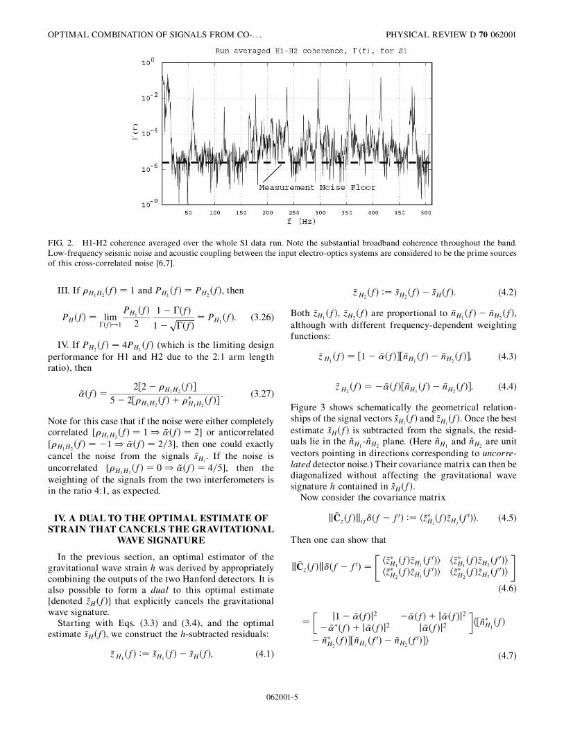
FIG. 2. H1-H2 coherence averaged over the whole S1 data run. Note the substantial broadband coherence throughout the band.Low-frequency seismic noise and acoustic coupling between the input electro-optics systems are considered to be the prime sourcesof this cross-correlated noise [6,7].


III. If �H1H2�f� � 1 and PH1

�f� � PH2�f�, then

PH�f� � lim�f�!1

PH1�f�

2

1� �f�

1��f�

p � PH1�f�: (3.26)

IV. If PH2�f� � 4PH1

�f� (which is the limiting designperformance for H1 and H2 due to the 2:1 arm lengthratio), then

~��f� �2�2� �H1H2

�f�

5� 2��H1H2�f� � �

H1H2�f�

: (3.27)

Note for this case that if the noise were either completelycorrelated [�H1H2

�f� � 1 ) ~��f� � 2] or anticorrelated[�H1H2

�f� � �1 ) ~��f� � 2=3], then one could exactlycancel the noise from the signals ~sHi

. If the noise isuncorrelated [�H1H2

�f� � 0 ) ~��f� � 4=5], then theweighting of the signals from the two interferometers isin the ratio 4:1, as expected.

IV. A DUAL TO THE OPTIMAL ESTIMATE OFSTRAIN THAT CANCELS THE GRAVITATIONAL

WAVE SIGNATURE

In the previous section, an optimal estimator of thegravitational wave strain h was derived by appropriatelycombining the outputs of the two Hanford detectors. It isalso possible to form a dual to this optimal estimate[denoted ~zH�f�] that explicitly cancels the gravitationalwave signature.

Starting with Eqs. (3.3) and (3.4), and the optimalestimate ~sH�f�, we construct the h-subtracted residuals:

~z H1�f� :� ~sH1

�f� � ~sH�f�; (4.1)

062001

~z H2�f� :� ~sH2

�f� � ~sH�f�: (4.2)

Both ~zH1�f�, ~zH2

�f� are proportional to ~nH1�f� � ~nH2

�f�,although with different frequency-dependent weightingfunctions:

~z H1�f� � �1� ~��f� �~nH1

�f� � ~nH2�f� ; (4.3)

~z H2�f� � �~��f��~nH1

�f� � ~nH2�f� : (4.4)

Figure 3 shows schematically the geometrical relation-ships of the signal vectors ~sHi

�f� and ~zHi�f�. Once the best

estimate ~sH�f� is subtracted from the signals, the resid-uals lie in the nH1

-nH2plane. (Here nH1

and nH2are unit

vectors pointing in directions corresponding to uncorre-lated detector noise.) Their covariance matrix can then bediagonalized without affecting the gravitational wavesignature h contained in ~sH�f�.

Now consider the covariance matrix

k~Cz�f�kij��f� f0� :� h~zHi�f�~zHj

�f0�i: (4.5)

Then one can show that

k~Cz�f�k��f� f0� �h~zH1

�f�~zH1�f0�i h~zH1

�f�~zH2�f0�i

h~zH2�f�~zH1

�f0�i h~zH2�f�~zH2

�f0�i

" #(4.6)

�j1� ~��f�j2 �~��f� � j~��f�j2

�~��f� � j~��f�j2 j~��f�j2

� �h�~nH1

�f�

� ~nH2�f� �~nH1

�f0� � ~nH2�f0� i

(4.7)

-5

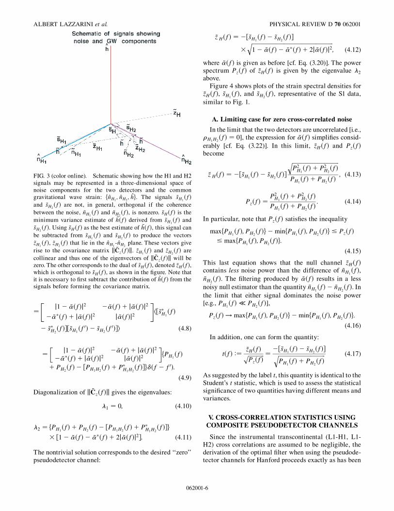
FIG. 3 (color online). Schematic showing how the H1 and H2signals may be represented in a three-dimensional space ofnoise components for the two detectors and the commongravitational wave strain: fnH1

; nH2; hg. The signals ~sH1

�f�and ~sH2

�f� are not, in general, orthogonal if the coherencebetween the noise, ~nH1

�f� and ~nH2�f�, is nonzero. ~sH�f� is the

minimum variance estimate of ~h�f� derived from ~sH1�f� and

~sH2�f�. Using ~sH�f� as the best estimate of ~h�f�, this signal can

be subtracted from ~sH1�f� and ~sH2

�f� to produce the vectors~zH1

�f�, ~zH2�f� that lie in the nH1

-nH2plane. These vectors give

rise to the covariance matrix k~Cz�f�k. ~zH1�f� and ~zH2

�f� arecollinear and thus one of the eigenvectors of k~Cz�f�k will bezero. The other corresponds to the dual of ~sH�f�, denoted ~zH�f�,which is orthogonal to ~sH�f�, as shown in the figure. Note thatit is necessary to first subtract the contribution of ~h�f� from thesignals before forming the covariance matrix.


�j1� ~��f�j2 �~��f� � j~��f�j2

�~��f� � j~��f�j2 j~��f�j2

" #h�~sH1

�f�

� ~sH2�f� �~sH1

�f0� � ~sH2�f0� i (4.8)

�j1� ~��f�j2 �~��f� � j~��f�j2

�~��f� � j~��f�j2 j~��f�j2

� �fPH1

�f�

� PH2�f� � �PH1H2

�f� � PH1H2

�f� g��f� f0�:

(4.9)

Diagonalization of k~Cz�f�k gives the eigenvalues:

�1 � 0; (4.10)

�2 � fPH1�f� � PH2

�f� � �PH1H2�f� � P

H1H2�f� g

� �1� ~��f� � ~��f� � 2j~��f�j2 : (4.11)

The nontrivial solution corresponds to the desired ‘‘zero’’pseudodetector channel:

062001

~z H�f� � ��~sH1�f� � ~sH2

�f�

��1� ~��f� � ~��f� � 2j~��f�j2

q; (4.12)

where ~��f� is given as before [cf. Eq. (3.20)]. The powerspectrum Pz�f� of ~zH�f� is given by the eigenvalue �2

above.Figure 4 shows plots of the strain spectral densities for

~zH�f�, ~sH1�f�, and ~sH2

�f�, representative of the S1 data,similar to Fig. 1.

A. Limiting case for zero cross-correlated noise

In the limit that the two detectors are uncorrelated [i.e.,�H1H2

�f� � 0], the expression for ~��f� simplifies consid-erably [cf. Eq. (3.22)]. In this limit, ~zH�f� and Pz�f�become

~z H�f� � ��~sH1�f� � ~sH2

�f�

��P2H1�f� � P2

H2�f�

qPH1

�f� � PH2�f�

; (4.13)

Pz�f� �P2H1�f� � P2

H2�f�

PH1�f� � PH2

�f�: (4.14)

In particular, note that Pz�f� satisfies the inequality

maxfPH1�f�; PH2

�f�g �minfPH1�f�; PH2

�f�g � Pz�f�

� maxfPH1�f�; PH2

�f�g:

(4.15)

This last equation shows that the null channel ~zH�f�contains less noise power than the difference of ~nH1

�f�,~nH2

�f�. The filtering produced by ~��f� results in a lessnoisy null estimator than the quantity ~nH1

�f� � ~nH2�f�. In

the limit that either signal dominates the noise power[e.g., PH1

�f� � PH2�f�],

Pz�f� ! maxfPH1�f�; PH2

�f�g �minfPH1�f�; PH2

�f�g:

(4.16)

In addition, one can form the quantity:

t�f� :�~zH�f��Pz�f�

p ��~sH1

�f� � ~sH2�f� ��

PH1�f� � PH2

�f�q (4.17)

As suggested by the label t, this quantity is identical to theStudent’s t statistic, which is used to assess the statisticalsignificance of two quantities having different means andvariances.

V. CROSS-CORRELATION STATISTICS USINGCOMPOSITE PSEUDODETECTOR CHANNELS

Since the instrumental transcontinental (L1-H1, L1-H2) cross correlations are assumed to be negligible, thederivation of the optimal filter when using the pseudode-tector channels for Hanford proceeds exactly as has been

-6

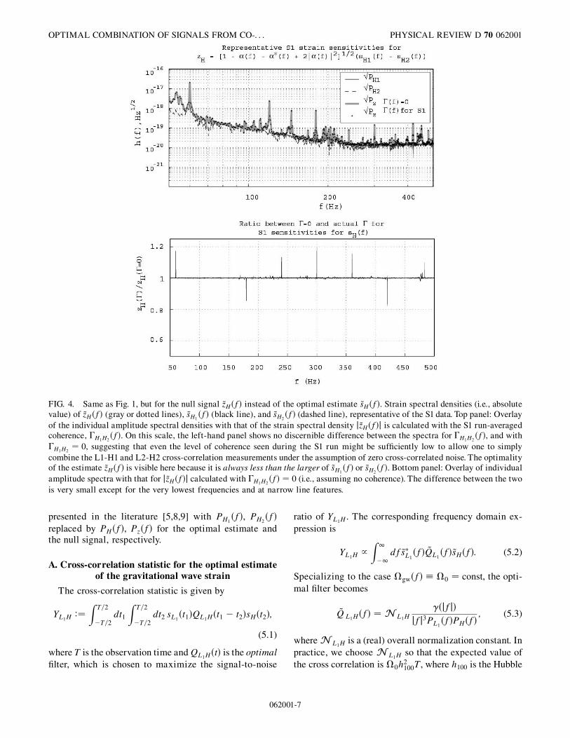
FIG. 4. Same as Fig. 1, but for the null signal ~zH�f� instead of the optimal estimate ~sH�f�. Strain spectral densities (i.e., absolutevalue) of ~zH�f� (gray or dotted lines), ~sH1

�f� (black line), and ~sH2�f� (dashed line), representative of the S1 data. Top panel: Overlay

of the individual amplitude spectral densities with that of the strain spectral density j~zH�f�j is calculated with the S1 run-averagedcoherence, H1H2

�f�. On this scale, the left-hand panel shows no discernible difference between the spectra for H1H2�f�, and with

H1H2� 0, suggesting that even the level of coherence seen during the S1 run might be sufficiently low to allow one to simply

combine the L1-H1 and L2-H2 cross-correlation measurements under the assumption of zero cross-correlated noise. The optimalityof the estimate ~zH�f� is visible here because it is always less than the larger of ~sH1

�f� or ~sH2�f�. Bottom panel: Overlay of individual

amplitude spectra with that for j~zH�f�j calculated with H1H2�f� � 0 (i.e., assuming no coherence). The difference between the two

is very small except for the very lowest frequencies and at narrow line features.


presented in the literature [5,8,9] with PH1�f�, PH2

�f�replaced by PH�f�, Pz�f� for the optimal estimate andthe null signal, respectively.

A. Cross-correlation statistic for the optimal estimateof the gravitational wave strain

The cross-correlation statistic is given by

YL1H:�

Z T=2

�T=2dt1

Z T=2

�T=2dt2 sL1

�t1�QL1H�t1 � t2�sH�t2�;

(5.1)

where T is the observation time and QL1H�t� is the optimalfilter, which is chosen to maximize the signal-to-noise

062001

ratio of YL1H. The corresponding frequency domain ex-pression is

YL1H /Z 1

�1df~sL1

�f� ~QL1�f�~sH�f�: (5.2)

Specializing to the case �gw�f� � �0 � const, the opti-mal filter becomes

~QL1H�f� � N L1H��jfj�

jfj3PL1�f�PH�f�

; (5.3)

where N L1H is a (real) overall normalization constant. Inpractice, we choose N L1H so that the expected value ofthe cross correlation is �0h2100T, where h100 is the Hubble

-7


expansion rate H0 in units of H100 :� 100 kms�1 Mpc�1.For such a choice,

N L1H �20 2

3H2100

�Z 1

�1df

�2�jfj�

f6PL1�f�PH�f�

��1: (5.4)

Moreover, one can show that the normalization factorN L1H and theoretical variance, �2

YL1H, of YL1H are related

by a simple numerical factor:

N L1H �1

T

3H2

100

5 2

��2

YL1H: (5.5)

1. Limiting case for white coherenceand PH1

�f� / PH2�f�

If the coherence is white [i.e., �H1H2�f� � const] and

the power spectra PH1�f�, PH2

�f� are proportional to oneanother, then one can show that the value of the cross-correlation statistic YL1H reduces to a linear combinationof the cross-correlation statistics YL1H1

and YL1H2calcu-

062001

lated separately for L1-H1 and L1-H2, if we allow forinstrumental correlations between H1 and H2. Thus, forthis case, combining the point estimates of �0 madeseparately for L1-H1 and L1-H2 gives the same resultas performing the coherent pseudodetector channelanalysis using the single optimal estimator ~sH�f�.

To show that this is indeed the case, note that�H1H2

�f� � const implies

H1H2�f� :� j�H1H2

�f�j2 � const: (5.6)

We will drop subscripts for constant quantities. If wefurther assume that PH2

�f� � �PH1�f�, then

PH1H2�f�

PH2�f�

��

p ;PH1H2

�f�

PH1�f�

� � ��

p: (5.7)

Thus, the integrand of the cross-correlation statistic,

YL1H�f�: � ~sL1�f� ~QL1H�f�~sH�f�; (5.8)

becomes

YL1H�f�

N L1H�

��f�~sL1�f�f~sH1

�f��PH2�f� � PH1H2

�f� � ~sH2�f��PH1

�f� � PH1H2

�f� g

jfj3PL1�f�PH1

�f�PH2�f��1� H1H2

�f� (5.9)

�1

1�

�1�

��

p

�YL1H1�f�

N L1H1

� �1� � ��

p�YL1H2

�f�

N L1H2

�; (5.10)

where the normalization factor Eq. (5.4) is

N L1H �20 2

3H2100

�Z 1

�1df

�2�jfj�fPH1�f� � PH2

�f� � �PH1H2�f� � P

H1H2�f� g

f6PL1�f�PH1

�f�PH2�f��1� H1H2

�f�

��1

(5.11)

� �1� ��

1��

p

�N �1

L1H1� �1� � ��

�p

�N �1L1H2

��1: (5.12)

Equivalently,

�2YL1H

� �1� ��

1��

p

��2

YL1H1� �1

� � ��

p��2

YL1H2

��1

(5.13)

� �1� ��2

YL1H1�2

YL1H2

�2YL1H1

�1� � ��

p� � �2

YL1H2�1� ��

�p �;

(5.14)

where we used Eq. (5.5) and similar equations to relateN L1H1

, N L1H2to �2

L1H1, �2

L1H2.

Substituting the above results for the normalizationfactors and variances into Eq. (5.10) and integratingover frequency, we find

YL1H ��2

YL1H

�1� �

�1�

��

p

� YL1H1

�2YL1H1

� �1� � ��

p�YL1H2

�2YL1H2

�(5.15)

��2

YL1H1�2

YL1H2

�2YL1H1

�1� � ��

p� � �2

YL1H2�1� ��

�p �

�1�

��

p

� YL1H1

�2YL1H1

� �1� � ��

p�YL1H2

�2YL1H2

�(5.16)

��2

YL1H2�1� ��

�p �YL1H1

� �2YL1H1

�1� � ��

p�YL1H2

�2YL1H1

�1� � ��

p� � �2

YL1H2�1� ��

�p �

:

(5.17)

Or in the notation of Appendix A:

-8

PHYSICAL REVIEW D 70 062001

YL1H ��C22 � C12�Y1 � �C11 � C21�Y2

C11 � C22 � C12 � C21; (5.18)

where Y1 :� YL1H1, Y2 :� YL1H2

, and where we usedEqs. (B1) and (B3) from Appendix B to equate �2

YL1H1,

�2YL1H2

with C11, C22, and PH1H2=PH2

� �=��

p,

PH1H2

=PH1� � ��

�p

with C12=C22, C21=C11. Thus, wesee that, for the limiting case of white coherence andproportional power spectra, the pseudodetector optimalestimator analysis reduces to a relatively simple combi-nation of the separate cross-correlation statisticmeasurements.

Finally, note that in the case of zero cross-correlatednoise [i.e., for �H1H2

�f� � 0] we get

YL1H ��2

YL1H2YL1H1

� �2YL1H1

YL1H2

�2YL1H1

� �2YL1H2

(5.19)

��2

YL1H1YL1H1

� ��2YL1H2

YL1H2

��2YL1H1

� ��2YL1H2

; (5.20)

which is the standard method of combining results ofmeasurements in the absence of correlations [6].

B. Cross-correlation statistic for the null signal

Once again, the cross-correlation statistic in the fre-quency domain is given by

YL1z /Z 1

�1df~sL1

�f� ~QL1z�f�~zH�f�: (5.21)

OPTIMAL COMBINATION OF SIGNALS FROM CO-. . .

062001

As before, the optimal filter for �gw�f� � �0 � const is

~QL1z�f� � N L1z��jfj�

jfj3PL1�f�Pz�f�

; (5.22)

where N L1z is chosen to be

N L1z �20 2

3H2100

�Z 1

�1df

�2�jfj�

f6PL1�f�Pz�f�

��1

(5.23)

and is related to the theoretical variance �2YL1z

via

N L1z �1

T

3H2

100

5 2

��2

YL1z: (5.24)

1. Limiting case for white coherence and PH1�f� /

PH2�f�

We start again with the same assumptions that thecoherence is white and the power spectra PH1

�f�, PH2�f�

are proportional to one another [cf. Eqs. (5.6), (5.7)]. Thenit is possible to show that the value of the cross-correlation statistic YL1z reduces to a linear combinationof the cross-correlation statistics YL1H1

and YL1H2calcu-

lated separately for L1-H1 and L1-H2, if we allow forinstrumental correlations between H1 and H2. Aftermuch algebra similar to that presented earlier inSec. VA 1 we obtain:

YL1z

�2YL1z

�

��3=2 � ��

q��

YL1H2

�2YL1H2

�YL1H1

�2YL1H1

��3=2 � �� 3 � 2j�j2 � �

��

p� �3=2��

q ; (5.25)

or, equivalently,

YL1z

�YL1z

�

��3=2 � �

��3=2 � �� 2 ��

p��

vuut �

YL1H2

�YL1H2

��

p YL1H1

�YL1H1

�(5.26)

�

��3=2 � �

��3=2 � ��1��

p��

��2 �

vuuut YL1H2� YL1H1��

�2YL1H2

� �2YL1H1

q �: (5.27)

2. Limiting case for zero cross-correlated noise

If also �H1H2�f� � 0, then the two interferometer noise

floors are uncorrelated, and the cross-correlation statisticYL1z for the null channel simplifies further:

YL1z

�L1z�

YL1H2� YL1H1��

�2YL1H1

� �2YL1H2

q : (5.28)

Equation (5.28) shows that in this limit the quantity

YL1z=�L1z follows the Student’s t distribution. Thisdistribution provides a measure to assess the significanceof the difference between two experimental quantitieshaving different means and variances. Here it provides ameasure of consistency of the two independent measure-ments, YL1H1

and YL1H2: Their difference should be con-

sistent with zero within the combined experimentalerrors.

-9


C. Combining triple and double coincidentmeasurements

In order to make use of this method for the analysis offuture science data, we will need to partition the data intothree nonoverlapping (hence statistically independent)sets: the H1-H2-L1 triple coincident data set, and thetwo L1-H1 and L1-H2 double coincident data sets. Thetriple coincidence data would be analyzed in the mannerdescribed in this paper, while the double coincidence data(corresponding to measurements from different epochs orfrom different science runs) can be simply combinedunder the assumption of statistical independence[cf. Eq. (5.20)].

VI. CONCLUSION

The approach presented above is fundamentally differ-ent from how the analysis of S1 data was conducted andrepresents a manner to maximally exploit the feature ofLIGO that has two colocated interferometers. This tech-nique is possible for the Hanford pair of detectors be-cause, to high accuracy, the gravitational wave signatureis guaranteed to be identically imprinted on both datastreams. Coherent, time-domain mixing of the two inter-ferometer strain channels can thus be used to optimaladvantage to provide the best possible estimate of thegravitational wave strain, and to provide a null channelwith which any gravitational wave analysis can be cali-brated for backgrounds.

An analogous technique of ‘‘time-delay interferome-try’’ (TDI) has been proposed in the context of the LaserInterferometer Space Array (LISA) concept [10,11].However, in that case the data analysis is very differentfrom what is explored in our paper. TDI involves timeshifting the six data streams of LISA (2 per arm) appro-priately before combining them so as to cancel (exactly)the laser-frequency noise that dominates other LISA noisesources. Even after implementing TDI, the resulting datacombinations (with the laser-frequency noise eliminated)are not all independent, and may have cross-correlatednoises from other, nongravitational-wave, sources. One,therefore, seeks in LISA data analysis an optimal strategyfor detecting a given signal in these TDI data combina-tions. On the other hand, the method presented in thispaper is not about canceling specific noise componentsfrom data; rather, it is about deducing the optimal detec-tion strategy in the presence of cross-correlated noise.

The usefulness of ~zH�f� is that it may be used toanalyze cross correlations for nongravitational-wave sig-nals between the Livingston and Hanford sites. Thiswould enable a null measurement to be made —i.e., onein which gravitational radiation had been effectively‘‘turned off.’’ In this sense, using ~zH�f� would be analo-gous to analyzing the ALLEGRO-L1 correlation whenthe orientation of the cryogenic resonant bar detectorALLEGRO is at 45� with respect to the interferometer

062001

arms [12,13]. Under suitable analysis, the cross-correlation statistic YL1z could be used to establish an‘‘off-source’’ background measurement for the stochasticgravitational wave background.

Ultimately, the usefulness of such a null test will berelated to how well the relative calibrations between H1and H2 are known. If the contributions of ~h�f� to ~sH1

�f�and ~sH2

�f� are not equal due to calibration uncertainties,then this error will propagate into the generation of ~sH�f�,~zH�f�. It is possible to estimate this effect as follows.Because of the intended use of ~zH�f� in a null measure-ment, the leakage of ~h�f� into this channel is the greaterconcern. Considering the structure of Eqs. (3.17), (4.3),and (4.4), it is clear that effects of differential calibrationerrors in ~sH�f� will tend to average out, whereas sucherrors will be amplified in ~zH�f�. Assume a differentialcalibration error of �~��f�. Then ~zH�f� will contain agravitational wave signature

�~h�f� � 2~��f�~h�f�; (6.1)

with corresponding power

�Ph�f� � 4j~��f�j2Ph�f�: (6.2)

The amplitude leakage affects single-interferometerbased analyses; the power leakage affects multiple inter-ferometer correlations (such as the stochastic backgroundsearch). Assuming reasonably small values for �~��f�, if asearch sets a threshold � on putative gravitational waveevents detected in channel ~sH�f�, then the correspondingcontribution in ~zH�f� would be approximately 2j�j�,where j�j denotes the magnitude of the frequency inte-grated differential calibration errors. For any reasonablethreshold (e.g., � � 10) above which one would claim adetection, and for typical differential calibration uncer-tainties of 2j�j & 20%, then the same event would have asignal-to-noise level of � � 2 in the null channel, wellbelow what one would consider meaningful. A morecareful analysis is needed to quantify these results, sincecalibration uncertainties also propagate into ~��f�.

While the focus of this paper is the application of thistechnique to the search for stochastic gravitational waves,it appears that any analysis can exploit this approach. Itshould be straightforward to tune pipeline filters and cullspurious events by using the null channel to veto eventsseen in the ~sH�f� channel.

ACKNOWLEDGMENTS

One of the authors (A. L.) wishes to thank SanjeevDhurandhar for his hospitality at IUCAA during whichthe paper was completed. He provided helpful insights bypointing out the geometrical nature of the signals andtheir inherent three-dimensional properties that span thespace fnH1

; nH2; hg. This led to an understanding of how

diagonalization of the covariance matrix could be

-10


achieved only after properly removing the signature of hfrom the interferometer signals. The authors gratefullyacknowledge the careful review and helpful suggestionsprovided by Nelson Christensen which helped finalizethe manuscript. This work was performed under partialfunding from the following NSF Grants: PHY-0107417,0140369, 0239735, 0244902, 0300609, and INT-0138459.J. D. R. and T. R. acknowledge partial support on PPARCGrant No. PPA/G/O/2001/00485. This document hasbeen assigned LIGO Laboratory Document No. LIGO-P040006-05-Z.

APPENDIX A: GENERAL METHOD OFCOMBINING MEASUREMENTS ALLOWING

FOR CROSS CORRELATIONS

In this appendix, we present a general method of com-bining measurements, allowing for possible correlationsbetween them. In the following appendix (Appendix A),this method is applied to the case of the L1-H1 and L1-H2cross-correlation statistic measurements, which are takenover the same observation period and which may containsignificant instrumental H1-H2 correlations.

It is important to emphasize that the method discussedin this appendix is not the same as the pseudodetectoroptimal estimator method discussed in the main text; thepseudodetector method combines the data at the level ofdata streams ~sH1

�f�, ~sH2�f� before optimal filtering, while

the method discussed here combines the data at the levelof the cross-correlation statistic measurements YL1H1

andYL1H2

—i.e., after optimal filtering of the individual datastreams. As such, the method described here is not opti-mal, in general, since it does not take advantage of thecommon gravitational wave strain component h present inH1 and H2. However, as shown in the main text, when thecross correlation �H1H2

�f� is white and the power spectraPH1

�f�, PH2�f� are proportional to one another, the pseu-

dodetector optimal estimator method reduces to themethod described here.

Consider then a pair of (real-valued) random variablesY1, Y2 with the same theoretical mean

� :� hY1i � hY2i; (A1)

and covariance matrix

kCk :�C11 C12

C21 C22

� �; (A2)

where

Cij: � h�Yi ��Yj ��i � hYiYji ��2: (A3)

Note that C12 � C21 since the Yi are real. The absence ofcross correlations corresponds to C12 � C21 � 0.

062001

Now form the weighted average

Yopt :�

Pi�iYiPj�j

: (A4)

It is straightforward to show that Yopt has theoreticalmean �opt � �, and theoretical variance

�2opt �

1

�Pk�k�

2

Xi

Xj

�iCij�j: (A5)

Now find the weighting factors �i that minimize thevariance of Yopt. The result is

�i �Xj

kCk�1ij ; (A6)

or, explicitly,

�1 �C22 � C12

detkCk; �2 �

C11 � C21

detkCk; (A7)

where detkCk :� C11C22 � C12C21.One can prove the above result by defining an inner

product

�A;B� :�Xi

Xj

AikCk�1ij Bj; (A8)

and rewriting the variance as

�2opt �

�C � �;C � ��C � �; 1�2

: (A9)

Then �2opt is minimized by choosing �i such that

C � �:�Xj

Cij�j � 1 (A10)

for all i.For such a choice,

��2opt �

Xi

�i �C11 � C22 � C12 � C21

detkCk; (A11)

Yopt

�2opt

��C22 � C12�Y1 � �C11 � C21�Y2

detkCk; (A12)

so

Yopt ��C22 � C12�Y1 � �C11 � C21�Y2

C11 � C22 � C12 � C21: (A13)

This is the desired combination.

APPENDIX B: APPLICATION OF THE GENERALMETHOD TO THE L1-H1, L1-H2 CROSS-

CORRELATION STATISTIC MEASUREMENTS

Here we apply the results of the previous appendix tothe L1-H1 and L1-H2 cross-correlation measurements.

-11


We let Y1 denote the cross-correlation statistic YL1H1for

the L1-H1 detector pair, and Y2 denote the cross-correlation statistic YL1H2

for L1-H2, and assume thatthe measurements are taken over the same observationperiod of duration T. (If the observations were over differ-ent times, then there would be no cross-correlation termsand a simple weighted average by ��2

i would suffice.) Weneed only calculate the components of the covariancematrix to apply the method described in the previousappendix.

To calculate the Cij, we assume (as in the main text)that the cross-correlated stochastic signal power P��f� issmall compared to the autocorrelated noise in theindividual detectors, and that there are no broadbandtranscontinental instrumental or environmental correla-tions—i.e., jPn

L1Hi�f�j is small compared to the autocor-

related noise, the cross-correlated stochastic signalpower, and the H1-H2 cross correlation jPH1H2

�f�j. Thenit is fairly straightforward to show that

C11 � �2L1H1

; C22 � �2L1H2

; (B1)

062001

and

C12

C11C22�

C21

C11C22

�1

T

3H2

100

10 2

�2 Z 1

�1df

�2�jfj�PH1H2�f�

f6PL1�f�PH1

�f�PH2�f�

:

(B2)

Note that the above integral is real since PH1H2��f� �

PH1H2

�f� and the integration is over all frequencies (bothpositive and negative).

If we further consider the limiting case definedby white coherence [i.e., �H1H2

�f� � const] and propor-tional power spectra [i.e., PH1

�f� / PH2�f�], then

PH1H2�f�=PH1

�f� and PH1H2

�f�=PH2�f� are both constant

with values

PH1H2

PH2

�C12

C22;

PH1H2

PH1

�C21

C11: (B3)

[1] B. Barish and R. Weiss, Phys. Today 52, No. 10, 44(1999); http://www.ligo.caltech.edu/

[2] B. Willke et al., Classical Quantum Gravity 19, 1377(2002); http://www.geo600.uni-hannover.de/

[3] B. Caron et al., Nucl. Phys. B (Proc. Suppl.) 54, 167(1997); http://www.virgo.infn.it/

[4] K. Tsubono, in 1st Edoardo Amaldi Conference onGravitational Wave Experiments, edited by E. Coccia,G. Pizzella, and F. Ronga (World Scientific, Singapore,1995), p. 112.

[5] B. Allen and J. D. Romano, Phys. Rev. D 59, 102001(1999).

[6] LIGO Scientific Collaboration, B. Abbott et al., Phys.Rev. D 69, 122004 (2004).

[7] Robert Schofield, LIGO Hanford Observatory (privatecommunication); also http://www.ligo.caltech.edu/docs/

G/G030330-00.pdf; http://www.ligo.caltech.edu/docs/G/G030641-00.pdf

[8] E. E. Flanagan, Phys. Rev. D 48, 2389 (1993).[9] B. Allen, in Proceedings of the Les Houches School on

Astrophysical Sources of Gravitational Waves, LesHouches, 1995, edited by J. A. Marck and J. P. Lasota(Cambridge University Press, Cambridge, England,1996), p. 373.

[10] M. Tinto, D. A. Shaddock, J. Sylvestre, and J.W.Armstrong, Phys. Rev. D 67, 122003 (2003).

[11] M. Tinto, F. Estabrook, and J.W. Armstrong, Phys. Rev.D 69, 082001 (2004).

[12] L. S. Finn and A. Lazzarini, Phys. Rev. D 64, 082002(2001).

[13] J. T. Whelan, E. Daw, I. S. Heng, M. P. McHugh, and A.Lazzarini, Classical Quantum Gravity 20, S689 (2003).

-12

physical review d, volume 70, 062001 optimal combination

Documents