Relationship between students’ online learning behavior and course performance:What contextual information matters?

Zhongzhou Chen , Mengyu Xu, Geoffrey Garrido, and MatthewW. GuthrieDepartment of Physics, University of Central Florida, 4111 Libra Drive, Orlando, Florida 32816, USA

and Department of Statistics and Data Science, University of Central Florida,4000 Central Florida Boulevard, Orlando, Florida 32816, USA

(Received 21 March 2020; accepted 22 May 2020; published 15 June 2020)

This study examines whether including more contextual information in data analysis could improve ourability to identify the relation between students’ online learning behavior and overall performance in anintroductory physics course. We created four linear regression models correlating students’ pass-fail eventsin a sequence of online learning modules with their normalized total course score. Each model takes intoaccount an additional level of contextual information than the previous one, such as student learningstrategy and duration of assessment attempts. Each of the latter three models is also accompanied by avisual representation of students’ interaction states on each learning module. We found that the bestperforming model is the one that includes the most contextual information, including instruction condition,internal condition, and learning strategy. The model shows that while most students failed on the mostchallenging learning module, those with normal learning behavior are more likely to obtain higher totalcourse scores, whereas students who resorted to guessing on the assessments of subsequent modules tendedto receive lower total scores. Our results suggest that considering more contextual information related toeach event can be an effective method to improve the quality of learning analytics, leading to more accurateand actionable recommendations for instructors.

DOI: 10.1103/PhysRevPhysEducRes.16.010138

I. INTRODUCTION

Online learning platforms provide a rich variety of dataon students’ learning behavior, enabling researchers toexplore the relation between learning behavior and learningoutcome, motivation, course completion, and other studentcharacteristics. For example, Kortemeyer [1,2] examinedboth the relation between frequency of material access andstudents’ course outcome and the relation between discus-sion forum posts and learning outcome; Formanek et al. [3]studied the relation between number of video views, dis-cussion forum participation, peer grading participation andstudents’ level of motivation and engagement in a massiveopen online course (MOOC); Lin et al. [4] correlatedstudents’ access of instructional videos with course perfor-mance. In the broader field of learning analytics, moresophisticated analytic methods and algorithms have beendeveloped to either identify patterns in students’ onlinelearning behavior [5–8] or predict academic achievementbased on large datasets [9–13].

Inmost of those studies, students’online learningbehavioris characterized by the count, frequency, or total duration ofone or more types of online learning events, such as thenumber of discussion forum posts or frequency of videoviews. However, the same type of learning event occurringunder different contexts could be generated by distinct typesof student learning behavior. For example, a failed problemsolving attempt followedbyone ormorevideo access or pageaccess events suggests that the student is trying to learn howto solve the problem, while a sequence of failed homeworkattempts without accessing relevant instructional materialscould imply that the student is randomly guessing, especiallywhen the duration of the attempts are short. However, bothkinds of failed attemptswould contribute equally to the countor frequency of problem attempt data. Gašević et al. [14]suggested three types of contextual conditions that can havesignificant impact on learning analytics, based onWinne andHadwin’s self-regulated learning model [15]: Instructioncondition: such as the course mode, course content, choiceof technology, and instructional design. Internal condition:such as the level of utilization of learning tools and thelearner’s level of prior knowledge. Learning products andstrategy: including learner’s strategy for completing learningtasks, and the quality of the learning product such asannotations or discussion posts.A number of recent studies have emphasized to varying

degrees the context in which online learning events took

Published by the American Physical Society under the terms ofthe Creative Commons Attribution 4.0 International license.Further distribution of this work must maintain attribution tothe author(s) and the published article’s title, journal citation,and DOI.

PHYSICAL REVIEW PHYSICS EDUCATION RESEARCH 16, 010138 (2020)

2469-9896=20=16(1)=010138(15) 010138-1 Published by the American Physical Society

place, in addition to the number or frequency of events. Forexample, Wilcox and Pollock [16] examined the impact offour types of contextual information associated withstudents’ answering of online conceptual assessments,Seaton et al. [17] looked at the impact of the time durationof resource access, and Alexandron et al. and Pallazo et al.[18,19] utilized time duration and IP address to detectpossible copying behavior in students’ problem-solvingevents. Seaton et al. [20] examined the difference inresource usage that took place when students are complet-ing different tasks in a MOOC.In this study, we ask the question: Can outcomes of

learning analytics be improved by considering more con-textual information associated with each learning event,without increasing the complexity of the analytic methods?We increased the contextual information associated witheach event in three steps, and demonstrated that each step ledto increasingly informative descriptions of students’ onlinelearning behavior, which enabled us to provide increasinglyaccurate answers to our second research question: How doesstudents’ overall performance in a physics course correlatewith their online learning behavior? In other words, dostudents that are often referred to as “struggling” in a physicscourse study online learning resources differently from thosewho perform well in the course, and if so, what are the mostcharacteristic differences?To answer this question, we collected students’ online

learning data from a sequence of 10 online learning modules(OLMs) which were assigned as homework to be completedover two weeks. Each module contains an instructionalcomponent and an assessment component with 1–2 prob-lems. Previous studies have shown that the mastery-basedlearning design of the OLMs can not only improve studentlearning outcome [21,22] but also increase the interpret-ability and information richness of learning data [23].The main events analyzed in the current study are the

outcomes of each module, as measured by passing, failing,or aborting the assessment component, resulting in 10events per student. For each pass-fail event, we extractedthree types of contextual information: where, when, andhow? More specifically,

1. Where was it: On which of the 10 modules did eachpass-fail event take place?

2. When did it happen: Did the pass-fail event takeplace before or after the student accessed theinstructional material in each module, and afterhow many attempts did the student choose to accessthe instructional material?

3. How did it happen: For each pass-fail event, howmuch time was spent on solving the problems?Multiple previous studies have linked abnormallyshort problem-solving duration with either randomguessing or answer copying [18,19,23–27].

Each context corresponds to one of the conditionsproposed by Gašević [14]: the “where” reflects the

instructional condition of online materials being organizedin a sequence of OLMs, the “when” reflects students’internal state of choosing whether to access the learningresources, and the “how” serves as one indication of thestrategy of producing the learning product.We refer to the combination of a pass-fail event and its

associated contextual information as an “interaction state,”or “state” for short. We created three different levels ofinteraction states with each level including additionalcontextual information than the previous level, as explainedin detail in Sec. III. B. Therefore, each level contains morestates than the previous one.Students’ overall performance in the course is measured

by their normalized final course score, which includesscores from homework, two midterms and one final exam,lab activities, and classroom clicker questions. The finalcourse scores directly determine students’ letter grade forthe course.Three linear regression models were constructed to

associate each of the three levels of interaction states withstudents’ final course score, as well as a baseline modelfor comparison. To address the issue of collinearity [28]between the large number of variables, we selected foreach model a subset of significant variables using a regu-larized linear regression algorithm LASSO [29], and recon-structed the linear models using those LASSO-selectedsubsets. Complementary to the linearmodels,we also plottedstudents’ transition between different states on neighboringmodules using a series of parallel coordinate graphs,which isan updated version of the data visualization scheme devel-oped in an earlier study [30]. As detailed in Sec. IV, acomplete description of student learning was obtained bycombining the linear model with the corresponding parallelcoordinate graph for each level.In Sec. V, we interpret and compare the outcomes of

analysis based on the three levels of interaction states, anddiscuss the benefit of including increasing amounts ofcontextual information on each event. We show that, in thiscase, the inclusion of more contextual information results inmore informative descriptions of students’ learning behav-ior. The model that includes all three types of contextualinformation reveals a characteristic difference in the waytop and bottom students complete certain OLMs, whichprovides the most accurate actionable recommendations forinstructors. We also discuss the implications of the currentresults for both instructors and education researchers, aswell as caveats and future directions of the current study.

II. STUDY SETUP

A. Design of OLM sequence

The OLM sequence is created using the Obojobolearning objects platform, developed as free and opensource software by the Center for Distributed Learningat University of Central Florida [31]. Each OLM consists of

CHEN, XU, GARRIDO, and GUTHRIE PHYS. REV. PHYS. EDUC. RES. 16, 010138 (2020)

010138-2

an instructional component (IC) and an assessment com-ponent (AC) (cf. Fig. 1). The AC contains 1–2 multiplechoice problems and allows a total of 5 attempts. Each ofthe first 4 attempts are sets of isomorphic problemsassessing the same physics knowledge but with differentsurface features or different numbers. On the 5th attempt,the same problem on the 1st attempt is presented to thestudents again. On four of the modules used in the currentstudy, a new set of isomorphic problems is presented tostudents on each of the first 3 attempts, while the sameproblems on the 1st and 2nd attempt were repeated on the4th and 5th attempts. Each IC contains a variety of learningresources, including text, figures, videos, and practiceproblems, focusing on explaining one or two basic con-cepts or introducing problem solving skills that are assessedby the problems in the AC. Upon opening a new module, astudent must make one attempt at the AC before beingallowed access to the IC. From a pedagogical perspective,the required first attempt could improve students’ learningfrom the IC [32], via the “preparation for future learning”effect [33]. From a research perspective, the first attemptserves as a de facto pretest that can measure students’incoming knowledge of the content.Access to the IC is locked whenever the student is

attempting the AC and is unlocked after the answers aresubmitted. Students are required to access the OLMsequence in the order given. In the 2017 implementation,due to platform limitations, students could access the nextmodule once they had submitted their 1st attempt on thecurrent module. However, students were not explicitlyinformed of that information, and were encouraged tocomplete the current module by either passing the AC orusing up all attempts before moving on to the next one. Wefound that in less than 3% of the cases a student accessedthe next module in sequence before passing the current one.Those events are excluded from the current analysis.The OLM sequence used in the current study consists of

10 modules covering the subject of work and mechanicalenergy. The first six modules introduce the conceptsof work, kinetic and potential energy, and conservation ofmechanical energy. The AC for those modules consistsof mostly conceptual questions (with the exception ofmodule 3, work and kinetic energy). Modules 7–10 focusedon solving increasingly complex mechanical energy prob-lems, and theACs consist of numerical calculation problems.

The problems in the AC are inspired by either commonhomework problems [34] or research-based assessmentinstruments [35]. Readers can access the OLM sequencefollowing the URL provided in Ref. [36]. Because of currentplatform limitations, all the problems were given in amultiple-choice format.

B. Implementation of the OLM sequence

The OLM sequencewas implemented in a large calculus-based college introductory physics course in fall of 2017,taught in a traditional lecture format. Of the 236 studentswho registered for the class, 184 were male and 52 werefemale, 107 were ethnic minorities.The OLM sequence was assigned to students as home-

work. Modules 1–6 were released one week before mod-ules 7–10, and all 10 modules were due 2.5 weeks after therelease of the first six modules. Completing all 10 moduleswas worth 9% of the total course score, and each modulewas weighted equally. The modules were released con-currently with classroom lectures on the same topic. Thecontents of the modules were tested on both the 2ndmidterm exam and the final exam of the course. No otherassignments were assigned to the students during the2.5 week period. A total of 230 students attempted at leastone module, and 223 students attempted all 10 modules.

III. METHODS

This section describes in detail how we first extractlearning events and contextual information from the rawclick-stream data, then integrate the learning events withincreasing amounts of contextual information to generatethree levels of interaction states for each module, with eachlevel containing one additional type of contextual infor-mation. We then describe the three linear regression modelscreated using the three levels of interaction states, plus abaseline model that includes only pass-fail events. We alsodescribe how we address the problem of collinearity withinvariables using LASSO.

A. Analysis of students’ click-stream data

Students’ click-stream data collected from the Obojoboplatform are analyzed using R and the tidyverse package[37,38]. For the current study, we extracted the followingtypes of information from the click-stream data:AC attempt outcome and duration.—An AC attempt is

recorded as “pass” if the student answers every questioncorrectly, otherwise it is recorded as “fail.” The duration ofeach attempt is recorded as the time between the studentclicks a button to start the attempt, and when the studentclicks another button to submit the answers.Study sessions.—A study session is defined as all

students’ interaction with the IC between two consecutiveAC attempts on a given module. The duration of a singlestudy session is the sum of all the events that took place

FIG. 1. Schematic illustration of the design of online learningmodule. Two modules in a sequence are shown.

RELATIONSHIP BETWEEN STUDENTS’ … PHYS. REV. PHYS. EDUC. RES. 16, 010138 (2020)

010138-3

during the session, including viewing page content andattempting practice problems. Since each module allows amaximum of 5 attempts, and require one attempt beforeallowing access to the IC, a student can have a maximum of4 study sessions. However, we observed that in 93% of thecases, each student only had one study session on a givenmodule. In only 6% of the cases did a student have a secondstudy session longer than 60 sec and at least 30% as long astheir longest study session in thatmodule. For those6%of thecases, we only consider the first of the two study sessions,which is usually the longer one. In the remaining 1% of thecases, the second (and 3rd) study session are neglectedbecause they are either shorter than 30% of the longest studysession, or last less than 60 sec. These choices are unlikely toimpact the outcome of the current analysis, because we onlyconsider whether a student had a study session, and howmany attempts were made before and after the study session,not the duration of each study session.

B. Students’ interaction states with OLMs

1. Defining interaction states with increasing levels ofcontextual information

Level I (3 states).—The first level of interaction statesincludes information on “where” a pass-fail event tookplace, i.e., whether a student passed or failed the AC of aspecific module. We define the following three interactionstates for each module:

• Pass (P): A student passes the AC within the first 3attempts. The reason for this choice is that (i) on fourof the modules the AC will provide a differentproblem only on the first 3 attempts, and will repeatthe 1st problem on the 4th attempt; (ii) many studentsdo not have the knowledge or skill to pass the AC ontheir 1st attempt, so they essentially have 2 attemptsafter studying the IC to be considered as pass, whichprovides some tolerance for “slips,” such as putting inthe wrong number in the calculator.

• Fail (F): Students who cannot pass the AC within thefirst 3 attempts. In other words, either passed on the4th or 5th attempt or failed on all 5 attempts.

• Abort (A): Students who did not pass the module anddid not use up all 5 attempts before moving on to thenext module.

Information of the specific module on which each stateoccurred is added by combining the module number withthe above states when constructing the linear regressionmodel, which is described in detail in Sec. III. C. 1.Level II (six states).—The second level adds information

on “when” a pass-fail event took place with respect to therelated study event, on top of the three states in level I.More specifically, we divided students according towhether their passing or failing of the AC took placebefore or after studying the IC. Table I lists the six states inthis level, with examples of common sequences of eventsbelonging to each state, using “S” to represent a studysession, and “P” or “F” to represent the outcome of eachattempt. All possible event sequences can be categorizedinto those six states.The rationale for dividing P and F states according to

whether the outcome is achieved before or after the studysession is straightforward: students who can pass themodule before studying are likely to have stronger incom-ing knowledge than those who passed after studying. Onthe other hand, those who studied immediately after thefirst or second failing attempt likely are more motivated tolearn than those who studied after more than 3 failedattempts or did not study at all.Level III (nine states).—The third level adds contextual

information on “how” each pass-fail event is generated byfurther dividing the BSP, ASP, and ASF states according tothe duration of the attempts. Different cutoff values havebeen proposed in several earlier studies to distinguishbetween an abnormally short attempt and a regular problemsolving attempt. In the current analysis, we estimated thecutoff to be 35 sec, by fitting the attempt durationdistribution using scale mixtures of skew-normal distribu-tion models, detailed in the next section. On modules 2 and6, the cutoffs are adjusted to 17 and 24 sec, respectively, onattempts after the study session due to shorter overallattempt durations. We assert that students who spent lessthan the cutoff times on an AC attempt are unlikely to haveput in an authentic effort to solve or even read theproblem body.Therefore, we divide each of the BSP, ASP, and ASF

states into two new states, based on if the students’ attemptsare classified as “brief” or “normal” based on their attemptdurations. For example, the BSP state is divided into

TABLE I. Definition of level II states. Note that “fail” states are defined as failing the first three attemps on eachmodule. The example column presents the most common event sequence for each state.

State name State label Definition Example

Before study pass BSP Pass with no study session fF;PgAfter study pass ASP Pass with study session before the 3rd attempt fF;S;F;PgAfter study fail ASF Fail with study session before the 3rd attempt fF;S;F;F;PgLate study LS Fail with study session after the 3rd attempt fF;F;F;S;F;PgNo study NS Fail with no study session fF;F;F;F; FgAbort AB Fail and did not use all 5 attempts fF;S;Fg

CHEN, XU, GARRIDO, and GUTHRIE PHYS. REV. PHYS. EDUC. RES. 16, 010138 (2020)

010138-4

BSP-B and BSP-N (before study pass-brief and beforestudy pass-normal). For BSP and ASP, the attempt durationis taken from the passing attempt which is also the lastattempt. On ASF, the duration is taken as the longest of thefirst 3 attempts. The resulting nine interaction states and therelation between the three levels are listed in Table II.Determining the duration cutoff between brief and normal

attempts.—Previous studies showed the cutoff between briefand normal attempts can be determined by fitting thedistribution of the problem-solving duration using multi-component mixture models (e.g., Refs. [39,40]), finding thecutoff between the shortest component and the secondshortest component as demonstrated in Fig. 2.In the current study, we fit the distribution of problem

solving duration from students’ 1st AC attempts collectedfrom all 10 modules, using scale mixtures of normal orskew-normal distributions, since previous studies havesuggested that students’ problem solving duration distri-bution are likely skewed [24,39,40]. There are two reasonsfor using the duration data from the 1st attempt. First,because students are required to make their 1st AC attemptbefore studying the IC, they are more likely to make arandom guess. Therefore, the population of brief attempts ismore similar to normal attmps,making it easier to separatethe short duration component from the rest of the data.

Second, on the 1st attempt, students who made a normalattempt must have read the problem text carefully, whereasstudents who made a brief attempt likely did not, leading toa larger difference in duration between the two compo-nents. On their 2nd and 3rd attempts, students may be ableto read the problem text faster on some modules where theproblems are more similar to the 1st attempt, resulting insmaller difference in duration. For those modules, thecutoff for 2nd and 3rd attempts are being adjusted (seebelow). The reason for aggregating the duration data fromall 10 modules is based on the assumption that briefattempts should be largely independent of the context ofthe problem, since the student was not actually solving it.Aggregating the duration data will increase the accuracy forestimating the cutoff.Model fitting is conducted with package mixsmsn [41],

and details are presented in the Appendix. Based on theresults from model fitting, the cutoff between brief andnormal attempts is initially set at 35 sec for all modules. Tocheck if this 35 sec uniform cutoff is reasonable for allmodules and all attempts, we compared it to the mean of thelog duration distribution of attempts made both before andafter a study session. We use the mean of log-durationdistribution since the distribution is approximately log-normal on many modules. Attempts longer than 7200 secare excluded as outliers. For attempts before the studysession, the mean log-durations of all modules are between70 and 200 sec, much longer than 35 sec, with hardermodules having shorter mean durations. For attempts afterthe study session, on two modules (2 and 6) the mean log-durations are 35 and 53 sec, respectively; only about half aslong as the duration of attempts before study on the samemodules. Both modules contain conceptual problems, andthe problems presented on the 2nd or 3rd attempt are verysimilar to the one on the 1st attempt. It is reasonable toassume that students can correctly solve the problem ontheir 2nd or 3rd attempt by looking at the new diagram andwithout fully reading the problem body again. Therefore,for those two modules, we treat the shortest 15% of theattempts as brief, and adjust the cutoffs to 17 and 24 sec,respectively, for attempts after study. On all other modules,the mean duration of attempts after study either increased ordecreased slightly (m4). Therefore the same 35 sec cutoff isused for all other modules except m2 and m6.

C. Modeling linear relation between interaction statesand total course score

1. Initial construction of linear models

We construct three linear regression models betweenstudents’ interaction states on each module and their finalcourse score for each of the three levels of interaction states,in the form of Eq. (1), where for the ith student, yi is thestandardized final course score with mean of 0 and standarddeviation of 1 (referred to as final course z score in the restof the paper), ϵi represents the “noise term” that accounts

TABLE II. Correspondence between level I, II, and III states.

Level I Level II Level III

P BSP BSP-NBSP-B

ASP ASP-NASP-B

F ASF ASF-NASF-B

LS LSNS NS

A AB AB

FIG. 2. Example of a mixture model fit of the durationhistogram of 1st attempts on all 10 modules combined, withmaximum duration of 350 sec. The blue line indicating the 35 seccutoff used in the current study.

RELATIONSHIP BETWEEN STUDENTS’ … PHYS. REV. PHYS. EDUC. RES. 16, 010138 (2020)

010138-5

for all other effects not explained by the interaction stateson the modules. We assume that ϵi are identical andindependently normally distributed with mean 0:

yi ¼ β0 þXS

s¼2

β1;sδi;1;s þXS

s¼2

β2;sδi;2;s þ � � �

þXS

s¼2

β10;sδi;10;s þ ϵi: ð1Þ

In the model above, δi;m;s are dummy variables withδi;m;s ¼ 1 if the ith student has interaction state s formodule m, and δi;m;s ¼ 0 otherwise, for i ¼ 1; 2;…; n;m ¼ 1; 2;…; 10, and s ¼ 1; 2;…; S. Here n ¼ 223 is thenumber of students who completed all 10 modules, and S isthe maximum number of interaction states defined in eachlevel of linear model. The variables δi;m;s combine infor-mation contained in the module number, such as differentcontent and difficulty of each module, with students’interaction states. Consequently, the model parameter β0represents the expected final course score for students in a“reference state” for every module, while βm;s measures thedifference in the final score by being in state s in modulemcompared to the reference state.For each of the three levels, the reference state is set to be

the first state with s ¼ 1. According to the three levels, westudy the effects with number of states S to be 3, 6, and, 9respectively. Specifically, the reference state is listed asfollows for each level.

I. Final course z score ∼ 3 states. Reference state: PII. Final course z score ∼ 6 states. Reference state: BSPIII. Final course z score ∼ 9 states. Reference state:

BSPNIn each level, the reference state is selected as the

interaction state that is most likely associated with thehighest level of content knowledge from an instructor’spoint of view. The intercept reflects the predicted finalcourse z-score if all modules are in the reference state.For comparison, we also create a baseline linear regres-

sion model between the number of modules a student failedand aborted and their final course score:

yi ¼ α0 þ αFxF;i þ αAxA;i þ ϵi; ð2Þ

where yi is the standardized final course z score for studenti and xF;i and xA;i are the number of modules the studentfailed or aborted, respectively. The parameter α0 stands forthe expected score of students who passed all modules andαF (and αA, respectively) represents the amount of pointsdecreased in the course final z score for failing (aborting,respectively) one more module.

2. Addressing collinearity within regression variablesusing LASSO

Collinearity and regularized regression.—To constructthe linear model (1), we are estimating p ¼ 10S − 9unknown coefficients; i.e., 21, 51, and 81, respectively,for levels I, II, and III. The fact that p is nonnegligible to thenumber of students n ¼ 207 can induce significant issue inthe regression. In particular, it is likely that the spaceconstructed by the predictors is (nearly) singular, whichmeans some of the covariates are (nearly) linear combina-tions of others. This issue is known as collinearity and it cancause a highly inaccurate and unstable [28], if not non-existent, model estimation since the ordinary least squaresolution of 1 relies on the assumption that the covariatespace is nonsingular. In the presence of collinearity, theestimated relationship can be spurious and redundant, asthe effect of one covariate can be replaced by the combi-nation of others.In remedy of the collinearity, we employ least absolute

shrinkage and selection operator (LASSO) estimation[29,42], assuming only a small proportion of the statessignificantly influence the final course score. The LASSOregression regularizes the estimation by imposing a penaltyof model size to the square sum of errors, defined as in thefollowing equation:

ðβ0; βÞ ¼ argminðβ0;βÞXn

i¼1

ðyi − β0 − δ⊤i βÞ2 þ λβ1; ð3Þ

where the vector δi ¼ ðδi;m;s; 1 ≤ m ≤ 10; 1 ≤ s ≤ SÞ⊤contains the binary state dummy variable for each statein all ten modules, and β contains the correspondingcoefficients. The tuning parameter λ controls the strengthof penalty in the model, and hence the sparsity of theestimation. We select λ by a tenfold cross validation withthe minimum mean squared error.LASSO estimation assumes that a small subset of β is

nonzero and is well known for its model selection con-sistency under certain conditions (cf., Ref. [43]). In otherwords, the estimator (3) is able to select the correct subsetof features relevant to the overall course score withhigh probability. That is, with a large sample size, model(3) selects the relevant models and states and excludes theirrelevant with probability near one. We use for featureselection and then regress the final course z-score againstthe selected modules and states. Assume only a subset ofinteraction states in all the modules are relevant to students’final performance in the course, denoted as S0 ¼ f1 ≤j ≤ p∶βj ≠ 0g. Let S0 ¼ f1 ≤ j ≤ p∶βj ≠ 0g be the indexset of significant features selected in Eq. (3) and δS0 be thedesign matrix for the corresponding modules and states. Weestimate the corresponding coefficients β⋆ from the follow-ing regression:

CHEN, XU, GARRIDO, and GUTHRIE PHYS. REV. PHYS. EDUC. RES. 16, 010138 (2020)

010138-6

y ¼ δ⊤S0β⋆ þ ϵ; ð4Þ

where y and ϵ are the vector form of the final course z scoreand noise respectively. Note that in Eq. ð4Þ the irrelevantstates are not included in the predictors.

D. Visualizing students’ transition between interactionstates in an OLM sequence

To visualize how students transition between interactionstates from one module to the next, we plot data from the 10modules on a sequence of nine parallel coordinate dia-grams, as shown in Figs. 3–5. The two vertical axes on eachof the nine diagrams represent the interaction states on twoadjacent modules. Each student is represented as a linestarting from one interaction state on the left axis andending on another interaction state on the right axis. One ormore overlapping lines form a path indicating a transition

between two interaction states on two adjacent modules,where a horizontal path means that one or more studentremained in the same state on the two modules. The studentpopulation is divided equally into top 1=3, middle 1=3, andbottom 1=3 cohorts according to their final course score,with each cohort plotted on its own sequence of parallelcoordinate diagrams. The most populated major paths thatadd up to half of the population within each cohort arehighlighted by a yellow line, with the line widths propor-tional to the size of the major path. The current visuali-zation scheme has two differences from the version in theearlier study [30]: 1. The ordering of states is now based onthe results of the linear model. States that are morefrequently correlated with lower course grades are placedlower on the graph, with reference state being placed at thetop of the graph. 2. Adjacent paths are no longer clusteredinto a single path, as it cannot be argued that adjacent statesare more similar to each other than distant states.

FIG. 3. Parallel coordinate graphs using level I (three) states.

FIG. 4. Parallel coordinate graphs using level II (six) states.

RELATIONSHIP BETWEEN STUDENTS’ … PHYS. REV. PHYS. EDUC. RES. 16, 010138 (2020)

010138-7

In addition, variables in the linear model selected by theLASSO estimation algorithm are highlighted by three typesof labels on the axis: hollow triangles represent selectedvariables with β⋆

S0not significantly different from zero,

solid squares represent variables with β⋆S0

significantly

different from 0 at α < 0.05 level, and solid spheresrepresent with β⋆

S0significantly different from 0 at α <

0.01 level. Selected variables with β⋆S0> 0 are represented

by dark cyan (#1A9F76) labels, and those with β⋆S0< 0 are

represented by pollo blue (#8DA0CB) labels. Each label isrepeated 3 times on the three graphs for the three cohorts.

IV. RESULTS

A. Baseline model

The intercept and coefficients of the baseline regressionmodel (adjusted R2 ¼ 0.18, F ¼ 16.21, p < 0.01) arelisted in Table III. As expected, the average final scorefor students who passed all modules differs significantlyfrom the average of all students, and the number of bothfailed and aborted modules are negatively correlated withfinal course score, with correlation coefficients signifi-cantly different from zero at α < 0.01 level.

B. Level I: Three interaction states

For level I (three states on each module), 17 out of 21variables are selected by the LASSO algorithm, resulting

in a linear model of adjusted R2 ¼ 0.20; F ¼ 4.07;df ¼ 189; p < 0.01. The coefficients of the model areshown in Table IV. Most of the variables are negativelycorrelated with the final score, which is expected since theP state is selected as the reference state for each module. Inaddition to the intercept, six variables have coefficients thatare significantly different from zero, in which five of thoseare on modules 6–10. This is likely because the difficultyof the modules increases towards the end of the sequence.Surprisingly, the F state on module 10 is positivelycorrelated with the final score, indicating that studentswith high final scores are more likely to fail on this module.On the parallel coordinate graph (Fig. 3), the three states

are ordered as P, F, A, since on all modules (except on m10)the coefficients for both F and A states are negative, with

FIG. 5. Parallel coordinate graphs using level III (nine) states.

TABLE III. Estimated coefficients and p values for the baselinelinear regression model (2).

State Coefficients (α) p

Intercept 0.74 0.00**F −0.15 0.00**A −0.32 0.00**

TABLE IV. Estimated coefficients and p values of regression(4) for the three-state model (level I).

Module State Coefficients (β⋆) p

NA Intercept 0.80 0.00**m1 A −0.14 0.61m1 F −0.24 0.08m2 A −0.31 0.49m2 F −0.13 0.36m3 F −0.06 0.72m4 A −0.50 0.03*m4 F −0.17 0.18m5 F −0.21 0.09m6 F −0.40 0.04*m7 A −0.48 0.01*m7 F −0.32 0.03*m8 A −0.36 0.29m8 F −0.17 0.19m9 A −0.52 0.24m9 F −0.30 0.02*m10 A −1.02 0.23m10 F 0.25 0.04*

CHEN, XU, GARRIDO, and GUTHRIE PHYS. REV. PHYS. EDUC. RES. 16, 010138 (2020)

010138-8

the A states being more negative. Four of the six significantvariables correspond to the start or end point of a majorpath. Of which, m7-A is on the end of a significant path inthe bottom cohort only; m7-F is at the junction of two majorpaths on all three cohorts; m9-F is on 2 major paths in thebottom cohort and one major path in the middle cohort;m10-F is on the end of a major path in the middlecohort only.

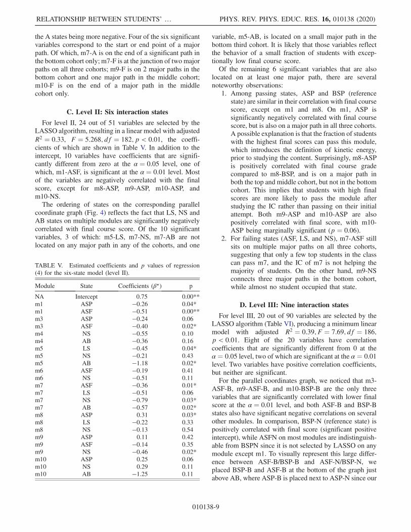
C. Level II: Six interaction states

For level II, 24 out of 51 variables are selected by theLASSO algorithm, resulting in a linear model with adjustedR2 ¼ 0.33, F ¼ 5.268; df ¼ 182; p < 0.01, the coeffi-cients of which are shown in Table V. In addition to theintercept, 10 variables have coefficients that are signifi-cantly different from zero at the α ¼ 0.05 level, one ofwhich, m1-ASF, is significant at the α ¼ 0.01 level. Mostof the variables are negatively correlated with the finalscore, except for m8-ASP, m9-ASP, m10-ASP, andm10-NS.The ordering of states on the corresponding parallel

coordinate graph (Fig. 4) reflects the fact that LS, NS andAB states on multiple modules are significantly negativelycorrelated with final course score. Of the 10 significantvariables, 3 of which: m5-LS, m7-NS, m7-AB are notlocated on any major path in any of the cohorts, and one

variable, m5-AB, is located on a small major path in thebottom third cohort. It is likely that those variables reflectthe behavior of a small fraction of students with excep-tionally low final course score.Of the remaining 6 significant variables that are also

located on at least one major path, there are severalnoteworthy observations:

1. Among passing states, ASP and BSP (referencestate) are similar in their correlation with final coursescore, except on m1 and m8. On m1, ASP issignificantly negatively correlated with final coursescore, but is also on a major path in all three cohorts.A possible explanation is that the fraction of studentswith the highest final scores can pass this module,which introduces the definition of kinetic energy,prior to studying the content. Surprisingly, m8-ASPis positively correlated with final course gradecompared to m8-BSP, and is on a major path inboth the top and middle cohort, but not in the bottomcohort. This implies that students with high finalscores are more likely to pass the module afterstudying the IC rather than passing on their initialattempt. Both m9-ASP and m10-ASP are alsopositively correlated with final score, with m10-ASP being marginally significant (p ¼ 0.06).

2. For failing states (ASF, LS, and NS), m7-ASF stillsits on multiple major paths on all three cohorts,suggesting that only a few top students in the classcan pass m7, and the IC of m7 is not helping themajority of students. On the other hand, m9-NSconnects three major paths in the bottom cohort,while almost no student occupied that state.

D. Level III: Nine interaction states

For level III, 20 out of 90 variables are selected by theLASSO algorithm (Table VI), producing a minimum linearmodel with adjusted R2 ¼ 0.39; F ¼ 7.69; df ¼ 186;p < 0.01. Eight of the 20 variables have correlationcoefficients that are significantly different from 0 at theα ¼ 0.05 level, two of which are significant at the α ¼ 0.01level. Two variables have positive correlation coefficients,but neither are significant.For the parallel coordinates graph, we noticed that m3-

ASF-B, m9-ASF-B, and m10-BSP-B are the only threevariables that are significantly correlated with lower finalscore at the α ¼ 0.01 level, and both ASF-B and BSP-Bstates also have significant negative correlations on severalother modules. In comparison, BSP-N (reference state) ispositively correlated with final score (significant positiveintercept), while ASFN on most modules are indistinguish-able from BSPN since it is not selected by LASSO on anymodule except m1. To visually represent this large differ-ence between ASF-B/BSP-B and ASF-N/BSP-N, weplaced BSP-B and ASF-B at the bottom of the graph justabove AB, where ASP-B is placed next to ASP-N since our

TABLE V. Estimated coefficients and p values of regression(4) for the six-state model (level II).

Module State Coefficients (β⋆) p

NA Intercept 0.75 0.00**m1 ASP −0.26 0.04*m1 ASF −0.51 0.00**m3 ASP −0.24 0.06m3 ASF −0.40 0.02*m4 NS −0.55 0.10m4 AB −0.36 0.16m5 LS −0.45 0.04*m5 NS −0.21 0.43m5 AB −1.18 0.02*m6 ASF −0.19 0.41m6 NS −0.51 0.11m7 ASF −0.36 0.01*m7 LS −0.51 0.06m7 NS −0.79 0.03*m7 AB −0.57 0.02*m8 ASP 0.31 0.03*m8 LS −0.22 0.33m8 NS −0.13 0.54m9 ASP 0.11 0.42m9 ASF −0.14 0.35m9 NS −0.46 0.02*m10 ASP 0.25 0.06m10 NS 0.29 0.11m10 AB −1.25 0.11

RELATIONSHIP BETWEEN STUDENTS’ … PHYS. REV. PHYS. EDUC. RES. 16, 010138 (2020)

010138-9

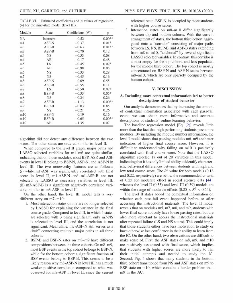
algorithm did not detect any difference between the twostates. The other states are ordered similar to level II.When compared to the level II graph, major paths and

LASSO selected variables for m1–m6 are quite similar,indicating that on those modules, most BSP, ASP, and ASFevents in level II belong to BSP-N, ASP-N, and ASF-N inlevel III. The two noteworthy features are as follows:(i) while m1-ASP was significantly correlated with finalscore in level II, m1-ASP-N and m1-ASP-B are notselected by LASSO as necessary variables in level III;(ii) m3-ASF-B is a significant negatively correlated vari-able, similar to m3-ASF in level II.On the other hand, the level III model tells a very

different story on m7–m10:1. Most interaction states on m7 are no longer selected

by LASSO for explaining the variance in the finalcourse grade. Compared to level II, in which 4 statesare selected with 3 being significant, only m7-NSis selected in level III, and the correlation is notsignificant. Meanwhile, m7-ASF-N still serves as a“hub” connecting multiple major paths in all threecohorts.

2. BSP-B and BSP-N sates on m8–m9 have differentcompositions between the three cohorts. On m8–m9,most BSP events in the top cohort belongs to BSP-N,while for the bottom cohort a significant fraction ofBSP events belong to BSP-B. This seems to be alikely reason why m8-ASP-N in level III has a muchweaker positive correlation compared to what wasobserved for m8-ASP in level II, since the current

reference state, BSP-N, is occupied by more studentswith higher course score.

3. Interaction states on m8–m10 differ significantlybetween top and bottom cohorts. With the currentarrangement of states, the bottom third cohort aggre-gated onto a “corridor” consisting of major pathsbetween LS, NS, BSP-B, andASF-B states extendingfrom m8 to m10, “anchored” by several significantLASSO selected variables. In contrast, this corridor isalmost empty for the top cohort, and less populatedfor the middle third cohort. The top cohort is mostlyconcentrated on BSP-N and ASP-N states betweenm8–m10, which are only sparsely occupied by thebottom cohort.

V. DISCUSSION

A. Including more contextual information led to betterdescriptions of student behavior

Our analysis demonstrates that by increasing the amountof contextual information associated with each pass-failevent, we can obtain more informative and accuratedescriptions of students’ online learning behavior.The baseline regression model [Eq. (2)] reveals little

more than the fact that high performing students pass moremodules. By including the module number information, thelevel I model shows that passing modules m6–m9 are betterindicators of higher final course score. However, it isdifficult to understand why failing on m10 is positivelycorrelated with final course score. Note that the LASSOalgorithm selected 17 out of 20 variables in this model,indicating that it has only limited ability to identify character-istic behavioral differences between students with high andlow total course score. The R2 value for both models (0.18and 0.22, respectively) are below the recommended criteriaof 0.25 for moderate effect in social science data [44],whereas the level II (0.33) and level III (0.39) models arewithin the range of moderate effects (0.25 < R2 < 0.64Þ.The level II states added the contextual information on

whether each pass-fail event happened before or afteraccessing the instructional materials. The level II modelreveals that on modules m5, m7, m8, and m9, students withlower final score not only have lower passing rates, but arealso more reluctant to access the instructional materialsafter repeated failure (LS and NS states). This could implythat those students either have less motivation to study orhave otherwise lost confidence in their ability to learn fromthe IC. On the other hand, two observations are difficult tomake sense of. First, the ASP states on m8, m9, and m10are positively associated with final score, which impliesthat students with higher scores are more likely to failtheir initial attempts and needed to study the IC.Second, Fig. 4 shows that many students in the bottomthird cohort transitioned from NS and ASF states on m9 toBSP state on m10, which contains a harder problem thanm9 in the AC.

TABLE VI. Estimated coefficients and p values of regression(4) for the nine-state model (level III).

Module State Coefficients (β⋆) p

NA Intercept 0.52 0.00**m1 ASF-N −0.37 0.01*m3 ASF-B −0.63 0.01**m3 ASP-B −0.70 0.12m4 NS −0.53 0.08m4 AB −0.17 0.48m5 LS −0.45 0.02*m5 AB −0.98 0.05m6 NS −0.33 0.28m7 NS −0.45 0.16m8 ASP-N 0.09 0.55m8 ASF-B −0.55 0.11m8 LS −0.50 0.02*m8 BSP-B −0.33 0.05*m8 NS −0.24 0.26m9 ASF-B −1.13 0.00**m9 BSP-B −0.03 0.85m9 NS −0.21 0.26m10 ASP-N 0.19 0.16m10 BSP-B −0.65 0.00**m10 AB −1.35 0.07

CHEN, XU, GARRIDO, and GUTHRIE PHYS. REV. PHYS. EDUC. RES. 16, 010138 (2020)

010138-10

The level III model included information on whetherthe pass-fail event was completed over a brief interval(less than 35 sec). The addition of this information seemsto be important for identifying characteristic behavioraldifferences between students with high and low final coursescores, as it allows the LASSO algorithm to select only 20out of 90 variables. The resulting model accounted for morevariance in the final course score using 4 fewer variablesthan the level II model.The level III parallel coordinate graph (Fig. 5) shows a

clear “corridor” from m8 to m10 for the bottom thirdcohort, consisting of major paths connecting either briefpassing attempts (BSP-B) or consecutive failed attemptswithout study (LS or NS). In contrast, the top third cohortmainly concentrated on normal passing attempts eitherbefore or after studying the IC (BSP-N and ASP-N) on thesame modules, whereas the middle third cohort has morefailed normal attempts (ASF-N). Remarkably, for all threecohorts, the major paths between m8-m10 all originatedfrom the same ASF-N state on m7. This observationsuggests that failing on m7 is not a characteristic differencebetween high and low performing students, but theirdifferent choices after experiencing the setback on m7is: while the top and most of the middle cohort continuedwith learning (with the middle cohort being less success-ful), most of the bottom cohort gave up and resorted toguessing on the following modules.The level III model also provides an explanation for the

anomalous observations on level I and II models: many Pand BSP events from the bottom 1=3 cohort on m9 and m10are BSP-B events (attempts shorter than 35 sec), while onlya few students in this cohort studied the IC of the module.Based on previous research [18,19,23,24], one possibleinterpretation is that students in the bottom 1=3 cohort aremore likely to have copied the answers to the problemsfrom another source.

B. Implications for instructors

One of the important goals of learning analytics is toprovide instructors with actionable recommendations toimprove student learning. In that regard, the level III modelis far superior to the other models.The simple baseline model and level I model both rely on

pass-fail events alone, which is similar towhat is provided bymany commercial online homework platforms. According tothese two models, the average instructor can do little morethan ask students to “work harder and pass more modules,especially onm6–m9.”The level IImodel suggests that somestudents might have lost confidence toward the end, but thepatterns are inconsistent. In addition, levels I and II modelscould mislead the instructor into believing that the bottomthird cohort eventually mastered the content or even out-performed the top and middle cohorts on m9 and m10.On the other hand, the level III model tells a more

complete and accurate story with three main takeaways:

1. On modules m1–m6, there are no qualitativedifferences in learning strategy for students withvarying levels of ability to succeed in the course.In other words, almost everyone is trying to learn inthe beginning.

2. Module 7 is challenging for most students as theinstructional materials are insufficient for helpingthem learning how to solve the problems in the AC.

3. After experiencing a setback on m7, students withlow course final scores are much more likely toemploy a guessing (or copying) strategy on the restof the modules.

Given those takeaways, rather than telling students to“study harder” or “do better,” a more helpful message couldbe “Everybody experiences setbacks—it is alright to fail!The key to success is to not give up.” In addition, twointerventions could potentially be beneficial for boostingstudents’ confidence:

1. Improve the quality of instruction on m7 to increasethe chance of success especially for low performingstudents.

2. Conduct activities that develop a growth mindset,which has been shown to be beneficial for studentsuccess [45–47].

Looking at the content of each module (which can beaccessed via [36]), m1–m6 mostly focused on introducingthe basic concepts of work and mechanical energy, whereasm7–m10 were designed to develop students’ ability tosolve numerical problems. The transition from conceptualunderstanding to mathematical modeling took placebetween m6, which contains two conceptual problemson the conservation of mechanical energy, and m7, whichcontains both a conceptual problem and a numericalcalculation problem on the same topic. Our results suggestthat this transition is very challenging for most students,and could have an impact on the confidence of somestudents. Therefore, instructors need to provide morescaffolding to facilitate students in this transition. Avaluable future direction will be to investigate if thedifficulty in the conceptual-mathematical transition canbe observed for other topics in introductory physics and inother learning environments.

C. Implications for researchers conducting data-drivenonline learning research

First of all, we demonstrated that instead of employingmore sophisticated algorithms, fine-tuning different param-eters, or using larger datasets, including detailed contextualinformation for each event analyzed can in some cases alsobe an effective approach for improving not only theaccuracy of data analysis models, but more importantlyin improving the ability to provide actionable and targetedinstructional suggestions for instructors.Second, this study highlights the importance of the

instructional design and platform capability in learning

RELATIONSHIP BETWEEN STUDENTS’ … PHYS. REV. PHYS. EDUC. RES. 16, 010138 (2020)

010138-11

analytics. The contextual data that are crucial for theconstruction of the level II and III models are groundedin the unique OLM design blending assessment withinstructional resources, which is made possible by theflexibility of the Obojobo platform. It is often the case thatplatform capability and instructional design can determineboth the variety and accuracy of information that can beextracted from student log data [22,48], and in turn limitsthe depth of learning analytics. For example, the RISEproject [49] is limited to simple analysis and visualizationwith limited contextual information, using data fromgeneric online learning platforms. Therefore, it can bebeneficial for all parties involved if data scientists andonline learning researchers play a more active role in thedesign, development, or adoption of online learning plat-forms and online courses, rather than passively stay on thereceiving end of educational data.

D. Caveats

One limitation of the current analysis is the use of auniversal 35 sec cutoff between brief and normal attempts.While this stringent criterion is favorable for avoiding falsepositives, it may not capture a significant number studentswho are not trying very hard on complex calculationproblems that cannot be correctly solved within severalminutes even by experts. This might explain why we stillobserve some students in the bottom cohort shift from latestudy and abort states on m9 to the BSP-N state on m10. Infact, for m9 and m10, exploratory data analysis [30]identified a separate distribution spending longer thanaverage time solving the problem, while achieving a bettercorrect response rate. Spending more than average time onthose problems could be a characteristic behavior of the top1=3 cohort just as brief problem solving is characteristic forthe bottom 1=3 cohort.Another imperfection of the current analysis is that the

scores on the OLM sequence are included in the totalfinal course grade, which violates the conditions for linearregression. However, we think that this is a negligiblesmall effect because (i) the OLM sequence only accountsfor 9% of the total grade and (ii) all students received atleast 90% of the score if they passed the module in 5attempts. As a result, the failed states used in the linearmodel do not directly correlate to the module scores.

E. General discussion and future directions

It is important to clarify that the purpose of the currentwork is not to create a predictive model for the course finalscore. Instead, our focus is on identifying and making senseof different behavior patterns among students with differentlevels of course performance, as well as demonstrating thevalue of integrating contextual information with events toobtain a more accurate and interpretable description ofstudent learning. This choice of focus provides justificationfor a number of decisions made in the current study.

First, we did not use one part of our data to generate theregression model and reserve other parts for verification, aswould be the standard process for creating a predictivemodel. Such an operation is not essential for identifyingand understanding students’ online learning behavior.Another reason is that not enough data was collected atthe time the analysis was conducted.Second, we chose the total final course score as the

dependent variable because it is the most straightforwardand generic way to classify high, middle, and low perform-ing students in a class, and is most suitable for answeringour research question. Student scores on a single assess-ment, or on part of an assessment related to the topic of themodule would be more suitable for a predictive model.Third, we chose to not include several types of available

data such as the time of each submission relative to thedue date, the number of practice problems solved duringlearning, or the demographics of the student population. Allof which could have improved the predictive power of themodel, but would not answer our research question.Although not a predictive model itself, the current study

is an essential first step towards creating better futurepredictive models. Existing predictive models are success-ful at identifying at-risk students with high accuracy, butoften have only limited ability to provide specific anduseful recommendations for both students and instructors.For example, students identified to be at-risk by the CourseSignal program receive little more than email and textmessages alerting them of their status [9]. The current studydemonstrated the possibility of overcoming such shortagesby collecting and integrating contextual information withindividual learning events.Another important question that the current study lays

the groundwork for answering is how the design of onlinelearning resources may shape students’ learning behaviorand learning outcomes. An actionable next step along thisdirection is to examine whether improvements recom-mended by the level III model could lead to detectablechanges in students’ enagagement pattern.Futhermore, the OLMs’ unique design allows for de

facto pretests and post-tests to be conducted on eachmodule [40], providing researchers with a new tool tomeasure students’ learning gains at much higher frequencythan existing methods. This could lead to new insight intothe relation between students’ learning behavior andlearning outcomes in an online environment. Much futurework is needed to either develop new analysis tools, oradopt similar existing methods [50] to properly measurelearning gain from OLM data.Finally, a more general question is whether including

contextual information could benefit the analysis of othertypes of data commonly studied in the field of physicseducation research. For example, we may be able to gainnew insight into students’ response data from standardassessment instruments, such as the Force Concept

CHEN, XU, GARRIDO, and GUTHRIE PHYS. REV. PHYS. EDUC. RES. 16, 010138 (2020)

010138-12

Inventory, by studying students’ response time on eachquestion, or considering the level to which classroominstruction is aligned with the test questions, using analysismethods similar to those developed in the current study.

ACKNOWLEDGMENTS

The authors would like to thank the Learning Systemsand Technology team at UCF for developing the Obojoboplatform. This research is partly supported by NSF GrantNo. DUE-1845436 and the Advancement of Early CareerResearchers (AECR) Program at the University of CentralFlorida.

APPENDIX: DETAILS ON DETERMINING THEBRIEF-NORMAL ATTEMPT DURATION CUTOFF

1. Skewed normal mixture model fitting

Mixture model data fitting is conducted using the fourdifferent distribution models available in the R packagemixsmsn: the normal distribution; the skew-normal distri-bution; the skew-Student-t distribution; and the skew-contaminated normal distribution (Skew-cn). The fittingalgorithm searches for the optimum number of componentsand fitting parameters for each distribution model accord-ing to model selection criteria EDC, which is shown to bemore reliable under certain conditions [51]. The four bestfit models are then compared based on four model selectioncriteria: AIC, BIC, EDC, and ICL. The model favored bythe most criteria is adopted. If more than one model isfavored, then the one favored by EDC is selected.One challenge for data fitting is that problem solving

durations can be as long as several thousand seconds,whereas Brief attempts are usually under 60 sec. Therefore,the best-fit model may be selected because of a good fit forthe long duration distribution but a less accurate fit for theshorter duration, or even not able to fit the short duration atall. To prevent this, we will only use the duration distri-bution below a maximum duration, and increase themaximum duration from 150 to 550 sec at 50 sec intervals

to examine how the maximum duration affects the estima-tion of the brief-normal cutoff distribution.The best fit model for each maximum duration, as well as

the estimated cutoff between the first and second compo-nent, is listed in Table VII. For maximum durationsbetween 200 and 300 sec, the multi-component skew-cndistribution is selected to be the best fit model, with the1st cutoff estimated at around 45 sec. When maximumdurations are more than 350 sec, the multi-componentnormal distribution is selected as the best fit model, with 1stcutoff at around 30 sec. However, the normal distributionsrun a higher risk of over fitting, since students’ problem-solving duration distribution should be skewed by nature,as there is always a minimum amount of time required tosolve any problem but no a clear upper limit. Therefore, wewill take 35 sec as our brief-norma cutoff, which is close tothe average of all the cutoffs obtained for different cutoffs.As shown in Fig. 6, the 35 sec cutoff sits right at the centerof the first minimum of the distribution.

2. Mean log-duration of attempts before and after study

In Table VIII, we list the mean log-duration (in unit ofseconds) of AC attempts both before and after studying theIC. Duration data is truncated at a maximum of 7200 sec.As shown in the table, modules m2 and m6 are the only twomodules on which the mean log-duration reduced by morethan a half from before study to after study. Therefore, thebrief-normal cutoff on those two modules for poststudyattempts are set at 17 and 24 sec, respectively, for afterstudy attempts. All other attempts used 35 sec as the brief-normal cutoff.

FIG. 6. Example of multicomponent mixture model fit of theduration distribution, with maximum duration of 350 sec. The redline indicates the cutoff generated by the algorithm at 30 sec, andthe blue line indicates the average cutoff for all durationsat 35 sec.

TABLE VIII. Mean log duration of before and after studyattempts for each module, in units of seconds.

Attempt type m1 m2 m3 m4 m5 m6 m7 m8 m9 m10

Before study 292 105 131 178 113 112 218 93 89 78After study 276 35 143 111 118 53 300 211 108 82

TABLE VII. Best fit model and the cutoff between the shortestand the next shortest distribution, for each maximum durationcutoff analyzed.

Max duration Model N components Cutoff (sec)

150 Skew.normal 3 33.5200 Skew.cn 3 46.5250 Skew.cn 4 43.5300 Skew.cn 4 48.5350 Normal 4 30.5400 Normal 4 30.5450 Normal 5 30.5500 Normal 5 31.5550 Normal 5 30.5

RELATIONSHIP BETWEEN STUDENTS’ … PHYS. REV. PHYS. EDUC. RES. 16, 010138 (2020)

010138-13

[1] G. Kortemeyer, Work habits of students in traditional andonline sections of an introductory physics course: A casestudy, J. Sci. Educ. Technol. 25, 697 (2016).

[2] G. Kortemeyer, Correlations between student discussionbehavior, attitudes, and learning, Phys. Rev. ST Phys.Educ. Res. 3, 010101 (2007).

[3] M. Formanek, S. Buxner, C. Impey, and M. Wenger,Relationship between learners’ motivation and courseengagement in an astronomy massive open online course,Phys. Rev. Phys. Educ. Res. 15, 020140 (2019).

[4] S. Y. Lin, J. M. Aiken, D. T. Seaton, S. S. Douglas, E. F.Greco, B. D. Thoms, and M. F. Schatz, Exploring physicsstudents’ engagement with online instructional videos in anintroductory mechanics course, Phys. Rev. Phys. Educ.Res. 13, 020138 (2017).

[5] J. Qiu, J. Tang, T. X. Liu, J. Gong, C. Zhang, Q. Zhang, andY. Xue, Modeling and predicting learning behavior inMOOCs, in Proceedings of the Ninth InternationalConference on Web Search and Data Mining—WSDM‘16 (ACM Press, New York, USA, 2016), pp. 93–102.

[6] R. F. Kizilcec, C. Piech, and E. Schneider, Deconstructingdisengagement: Analyzing learner subpopulations in mas-sive open online courses, ACM International ConferenceProceeding Series (2013), pp. 170–179, https://doi.org/10.1145/2460296.2460330.

[7] I. Borrella, S. Caballero-Caballero, and E. Ponce-Cueto,Predict and intervene: Addressing the dropout problem in aMOOC-based program, in Proceedings of the Sixth ACMConference on Learning @ Scale—L@S ‘19 (ACM Press,New York, USA, 2019), pp. 1–9.

[8] R. Martinez-Maldonado, K. Yacef, J. Kay, A. Kharrufa,and A. Al-Qaraghuli, Analysing frequent sequential pat-terns of collaborative learning activity around an interactivetabletop, in EDM 2011—Proceedings of the 4thInternational Conference on Educational Data Mining,Eindhoven, The Netherlands (2011), pp. 111–120.

[9] K. E. Arnold, M. D. Pistilli, and K. E. Arnold, Coursesignals at Purdue: Using learning analytics to increasestudent success, in 2nd International Conference onLearning Analytics and Knowledge, Vancouver, BC, Can-ada (2012), p. 2.

[10] J. W. You, Identifying significant indicators using LMSdata to predict course achievement in online learning,Internet High. Educ. 29, 23 (2016).

[11] Y. Li, C. Fu, and Y. Zhang, When and who at risk? Callback at these critical points, in Proceedings of the 10thInternational Conference on Educational Data Mining,Wuhan, China (2017), pp. 168–173.

[12] S. M. Jayaprakash, E. W. Moody, E. J. M. Lauria, J. R.Regan, and J. D. Baron, Early alert of academically at-riskstudents: An open source analytics initiative, J. Learn.Anal. 1, 6 (2014).

[13] R. S. Baker, D. Lindrum, M. J. Lindrum, and D. Perkowski,Analyzing early at-risk factors in higher educatione- learning courses, in Proceedings of the 8th InternationalConference on Educational Data Mining, Madrid, Spain(2015), p. 150.

[14] D. Gaševic, S. Dawson, and G. Siemens, Let’s not forget:Learning analytics are about learning, TechTrends 59, 64(2015).

[15] P. H. Winne and A. F. Hadwin, Studying as Self-RegulatedLearning, in Metacognition in Educational Theory andPractice, edited by D. J. Hacker, J. Dunlosky, and A. C.Graesser (Lawrence Erlbaum Associates Publishers,Mahwah, NJ, 2017).

[16] B. R. Wilcox and S. J. Pollock, Investigating students’behavior and performance in online conceptualassessment, Phys. Rev. Phys. Educ. Res. 15, 020145(2019).

[17] D. T. Seaton, G. Kortemeyer, Y. Bergner, S. Rayyan, andD. E. Pritchard, Analyzing the impact of course structureon electronic textbook use in blended introductory physicscourses, Am. J. Phys. 82, 1186 (2014).

[18] G. Alexandron, J. A. Ruiperez-Valiente, Z. Chen, P. J.Muñoz-Merino, and D. E. Pritchard, Copying @ Scale:Using harvesting accounts for collecting correct answers ina MOOC, Comput. Educ. 108, 96 (2017).

[19] D. J. Palazzo, Y. J. Lee, R. Warnakulasooriya, and D. E.Pritchard, Patterns, correlates, and reduction of home-work copying, Phys. Rev. ST Phys. Educ. Res. 6, 010104(2010).

[20] D. T. Seaton, Y. Bergner, I. Chuang, P. Mitros, and D. E.Pritchard, Who does what in a massive open onlinecourse?, Commun. ACM 57, 58 (2014).

[21] B. Gutmann, G. E. Gladding, M. Lundsgaard, and T.Stelzer, Mastery-style homework exercises in introductoryphysics courses: Implementation matters, Phys. Rev. Phys.Educ. Res. 14, 010128 (2018).

[22] M.W. Guthrie and Z. Chen, Adding duration-basedquality labels to learning events for improved descriptionof students’ online learning behavior, in Proceedings of the12th International Conference on Educational Data Min-ing, edited by M. C. Desmarais, C. F. Lynch, A. Merceron,and R. Nkambou (International Educational Data MiningSociety, Montreal, Canada, 2019).

[23] Z. Chen, S. Lee, and G. Garrido, Re-designing the structureof online courses to empower educational data mining, inProceedings of the 11th International Conference onEducational Data Mining, edited by K. Elizabeth Boyerand M. Yudelson (Buffalo, NY, 2018), pp. 390–396.

[24] R. Warnakulasooriya, D. J. Palazzo, and D. E. Pritchard,Time to completion of web-based physics problems withtutoring, J. Exp. Anal. Behav. 88, 103 (2007).

[25] C. L. Barry, S. J. Horst, S. J. Finney, A. R. Brown, and J. P.Kopp, Do examinees have similar test-taking effort? Ahigh-stakes question for low-stakes testing, Int. J. Non-destr. Test. 10, 342 (2010).

[26] S. L. Wise and X. Kong, Response time effort: A newmeasure of examinee motivation in computer-based tests,Appl. Meas. Educ. 18, 163 (2005).

[27] S. L. Wise, D. A. Pastor, and X. J. Kong, Correlates ofrapid-guessing behavior in low-stakes testing: Implicationsfor test development and measurement practice, Appl.Meas. Educ. 22, 185 (2009).

[28] E. J. Theobald, M. Aikens, S. Eddy, and H. Jordt, Beyondlinear regression: A reference for analyzing common datatypes in discipline based education research, Phys. Rev.Phys. Educ. Res. 15, 020110 (2019).

[29] R. Tibshirani, Regression shrinkage and selection via theLASSO, J. R. Stat. Soc. Ser. B 58, 267 (1996).

CHEN, XU, GARRIDO, and GUTHRIE PHYS. REV. PHYS. EDUC. RES. 16, 010138 (2020)

010138-14

[30] G. Garrido, M.W. Guthrie, and Z. Chen, How are students’online learning behavior related to their course outcomes inan introductory physics course?, in Proceedings of the2019 Physics Education Research Conference, Provo,UT, edited by Y. Cao, S. Wolf, and M. B. Bennett (AIP,New York, 2019).

[31] Center for Distributed Learning, Obojobo, https://next.obojobo.ucf.edu/.

[32] J. W. Morphew, G. E. Gladding, and J. P. Mestre, Effect ofpresentation style and problem-solving attempts on meta-cognition and learning from solution videos, Phys. Rev.Phys. Educ. Res. 16, 010104 (2020).

[33] D. L. Schwartz and J. D. Bransford, Efficiency and in-novation in transfer, in Transfer of Learning from aModern Multidisciplinary Perspective (Current Perspec-tives on Cognition, Learning and Instruction), edited byJ. P. Mestre (IAP - Informaiton Age Publishing Inc,Charlotte, NC, 2005), pp. 1–51.

[34] W. Fakcharoenphol, E. Potter, and T. Stelzer, What studentslearn when studying physics practice exam problems, Phys.Rev. ST Phys. Educ. Res. 7, 010107 (2011).

[35] C. Singh and D. Rosengrant, Multiple-choice test ofenergy and momentum concepts, Am. J. Phys. 71, 607(2003).

[36] Z. Chen, Obojobo Sample Canvas Course, https://canvas.instructure.com/courses/1726856.

[37] H. Wickham et al., Welcome to the Tidyverse, J. OpenSource Software 4, 1686 (2017).

[38] R Core Team, R: A language and environment forstatistical computing, www.r-Project.Org (2019).

[39] D. L. Schnipke and D. J. Scrams, Modeling item responsetimes with a two-state mixture model- a new approach tomeasuring speededness, J. Educ. Measure. 34, 213 (1997).

[40] Z. Chen, G. Garrido, Z. Berry, I. Turgeon, and F. Yonekura,Designing online learning modules to conduct pre- andpost-testing at high frequency, in Proceedings of the 2017Physics Education Research Conference, Cincinnati, OH(AIP, New York, 2018), pp. 84–87.

[41] M. O. Prates and C. R. B. Cabral, Mixsmsn: Fitting finitemixture of scale mixture of skew-normal distributionsmarcos, J. Stat. Softw. 30, 1 (2009).

[42] J. Friedman, T. Hastie, and R. Tibshirani, Regularizationpaths for generalized linear models via coordinate descent,J. Stat. Softw. 33, 1 (2010).

[43] P. Zhao and Y. Bin, On model selection consistency ofLASSO, J. Mach. Learn. Res. 7, 2541 (2006).

[44] C. J. Ferguson, An effect size primer: A guide for cliniciansand researchers, Prof. Psychol. Res. Pract. 40, 532 (2009).

[45] D. S. Yeager, D. Paunesku, G. M. Walton, and C. S.Dweck, Excellence in education: The importance ofacademic mindsets, inWhite Paper prepared for the WhiteHouse meeting on Excellence in Education: The Impor-tance of Academic Mindsets 42 (2013).

[46] S. Claro, D. Paunesku, and C. S. Dweck, Growth mindsettempers the effects of poverty on academic achievement,Proc. Natl. Acad. Sci. U.S.A. 113, 8664 (2016).

[47] C. S. Dweck and E. L. Leggett, A social-cognitive ap-proach to motivation and personality, Psychol. Rev. 95, 256(1988).

[48] M.W. Guthrie and Z. Chen, Comparing student behaviorin mastery and conventional style online physics home-work, in Proceedings of the 2019 Physics EducationResearch Conference, Provo, UT, edited by Y. Cao, S.Wolf, and M. B. Bennett (AIP, New York, 2019).

[49] R. Bodily, R. Nyland, and D. Wiley, The RISE framework:Using learning analytics to automatically identify openeducational resources for continuous improvement, Int.Rev. Res. Open Distance Learn. 18, 103 (2017).

[50] Y. J. Lee, D. J. Palazzo, R. Warnakulasooriya, and D. E.Pritchard, Measuring student learning with item responsetheory, Phys. Rev. ST Phys. Educ. Res. 4, 010102 (2008).

[51] C. C. Y. Dorea, P. A. A. Resende, and C. R. Gonçalves,Comparing the Markov order estimators AIC, BIC andEDC, in Transactions on Engineering Technologies:World Congress on Engineering and Computer Science2014 (Springer Netherlands, 2015), pp. 41–54.

RELATIONSHIP BETWEEN STUDENTS’ … PHYS. REV. PHYS. EDUC. RES. 16, 010138 (2020)

010138-15