Physics 7450: Solid State Physics 2

Lecture 2: Elasticity and phonons

Leo Radzihovsky

(Dated: 12 January, 2015)

Abstract

In these lecture notes, starting with semi-microscopic model of a crystal we will develop a generic

discrete model of crystalline elasticity. We will study quantum and thermal fluctuations governed

by this elastic Hamiltonian within the discrete and continuum elastic limits. We will conclude with

the study of effects of elastic nonlinearities.

1

I. CRYSTAL LATTICE IN HARMONIC APPROXIMATION

A. General discrete formulation

As discussed in lecture 1, interacting ions forms a lattice, characterized by (in general)

quantum coordinates Ri with a Hamiltonian

Hion =N∑i

P2i

2Mi

+1

2

N∑i,j

Upair(|Ri −Rj|), (1)

where Upair(R) is the inter-ionic pair potential that we have approximated to be of central

force type, depending only on the inter-atomic distance R and not on the bond angles. Al-

though microscopically it is simply the Coulomb potential, because of the screening effects

by the electrons we have taken it to be a generic function with a minimum that by construc-

tion gives a particular equilibrium crystal structure, Ri = Rn,s (recall that n = (n1, n2, n3)

labels Bravais lattice sites and s p-atom basis within the unit cell). The calculation of the

latter requires quite involved first-principles numerical analysis that we will avoid here and

package that information into Upair.

The full quantum description of the crystal structure is then formulated in terms of

deviations us(n) ≡ u(Rn,s) ≡ uR from this perfect crystalline structure

Ri = Rn,s + u(Rn,s). (2)

For small fluctuations, we can employ the harmonic approximation, Taylor-expanding a

generic ionic potential energy

U(Ri) = U0 +1

2

∑m,n;s,t;α,β

U s,tα,β(m,n)us

α(m)utβ(n), (3)

= U0 −1

4

∑m,n;s,t;α,β

U s,tα,β(m− n)(us

α(m)− utα(n))(us

α(m)− utα(n)), (4)

where U0 ≡ U(Rn,s), Us,tα,β(m − n) ≡ ∂2U

∂usα(m)∂ut

β(n), the linear term vanished by virtue of the

expansion around the minimum Rn,s, dependence on m− n is due to discrete lattice trans-

lational invariance, and in the last equality we utilized the continuous uniform translational

invariance of the whole crystal, us(m) → us(m) + ε, which requires∑

m,s Us,tα,β(m,n) = 0

(vanishing energy of uniform translation).

2

An equivalent description (but slightly less general since it is possible for the interaction

not to be purely pairwise-additive or be of purely central form) is in terms of the pair

potential Upair(|Rij|):

U(Ri) =1

2

N,p∑Rm,s,Rn,t

Upair(|Rm,s −Rn,t + u(Rm,s)− u(Rn,t)|), (5)

≈ U0 +1

4

N,p∑R,R′

U s,tαβ(|R−R′|)(uα

R − uαR′)(u

βR − uβ

R′), (6)

≈ U0 +1

2

∑k∈BZ

Ds,tαβ(k)uα

−k,suβk,t (7)

where with r ≡ |Rm,s −Rn,t|, we have force constants matrix given by

U s,tαβ(r) = δαβ

1

r

∂Upair(r)

∂r+

(∂2Upair(r)

∂r2− 1

r

∂Upair(r)

∂r

)rαrβ

r2, (8)

and its Fourier transform, the dynamical matrix

Ds,tαβ(k) =

N∑Rn

U s,tαβ(|Rm,s −Rn,t|)

(1− eik·(Rm,s−Rn,t)

), (9)

Within this harmonic approximation the equation of motion together with the kinetic

energy

Tkin =∑R

1

2Msu

2R, (10)

=∑R

P2R

2Ms

, (11)

is straightforwardly obtained (via Hamiltonian or Lagrangian formalisms):

MsuαRm,s

= −N,p∑Rn,t

U s,tαβ(|Rm,s −Rn,t|)(uβ

Rm,s− uβ

Rn,t)

which in 3d corresponds to 3Np coupled harmonic oscillator equations. Because of discrete

(lattice) translational symmetry, as we will see these can be decoupled using normal modes

that are nothing else but the Fourier series coefficients labelled by 3Np discrete values of k.

B. One-dimensional atomic chain

1. Normal modes decoupling

To get a feel for these expressions as a warm-up we will first consider a 1d monoatomic

(no basis, p = 1), harmonic chain, illustrated in Fig.(1).

3

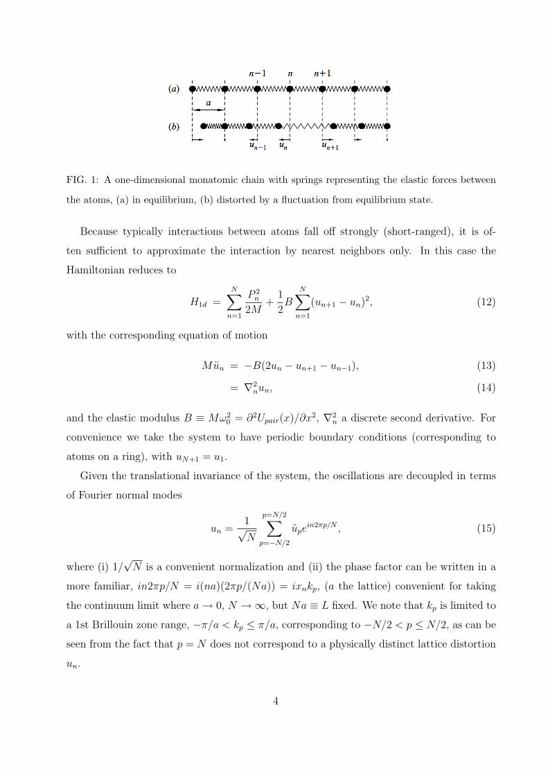
FIG. 1: A one-dimensional monatomic chain with springs representing the elastic forces between

the atoms, (a) in equilibrium, (b) distorted by a fluctuation from equilibrium state.

Because typically interactions between atoms fall off strongly (short-ranged), it is of-

ten sufficient to approximate the interaction by nearest neighbors only. In this case the

Hamiltonian reduces to

H1d =N∑

n=1

P 2n

2M+

1

2B

N∑n=1

(un+1 − un)2, (12)

with the corresponding equation of motion

Mun = −B(2un − un+1 − un−1), (13)

= ∇2nun, (14)

and the elastic modulus B ≡ Mω20 = ∂2Upair(x)/∂x

2, ∇2n a discrete second derivative. For

convenience we take the system to have periodic boundary conditions (corresponding to

atoms on a ring), with uN+1 = u1.

Given the translational invariance of the system, the oscillations are decoupled in terms

of Fourier normal modes

un =1√N

p=N/2∑p=−N/2

upein2πp/N , (15)

where (i) 1/√N is a convenient normalization and (ii) the phase factor can be written in a

more familiar, in2πp/N = i(na)(2πp/(Na)) = ixnkp, (a the lattice) convenient for taking

the continuum limit where a→ 0, N →∞, but Na ≡ L fixed. We note that kp is limited to

a 1st Brillouin zone range, −π/a < kp ≤ π/a, corresponding to −N/2 < p ≤ N/2, as can be

seen from the fact that p = N does not correspond to a physically distinct lattice distortion

un.

4

Using this representation inside the equation of motion, and also Fourier transforming in

time, we find

−Mω2uk(ω) = −B(2− e−ika − eika)uk(ω), (16)

= −2B(1− cos ka)uk(ω), (17)

which gives the acoustic phonon dispersion

ω(k) =

√2B

M(1− cos ka) = 2

(B

M

)1/2

| sin(1

2ka)|, (18)

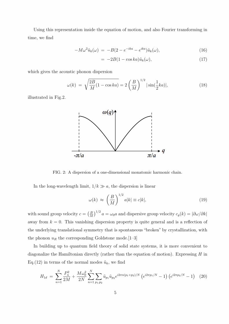
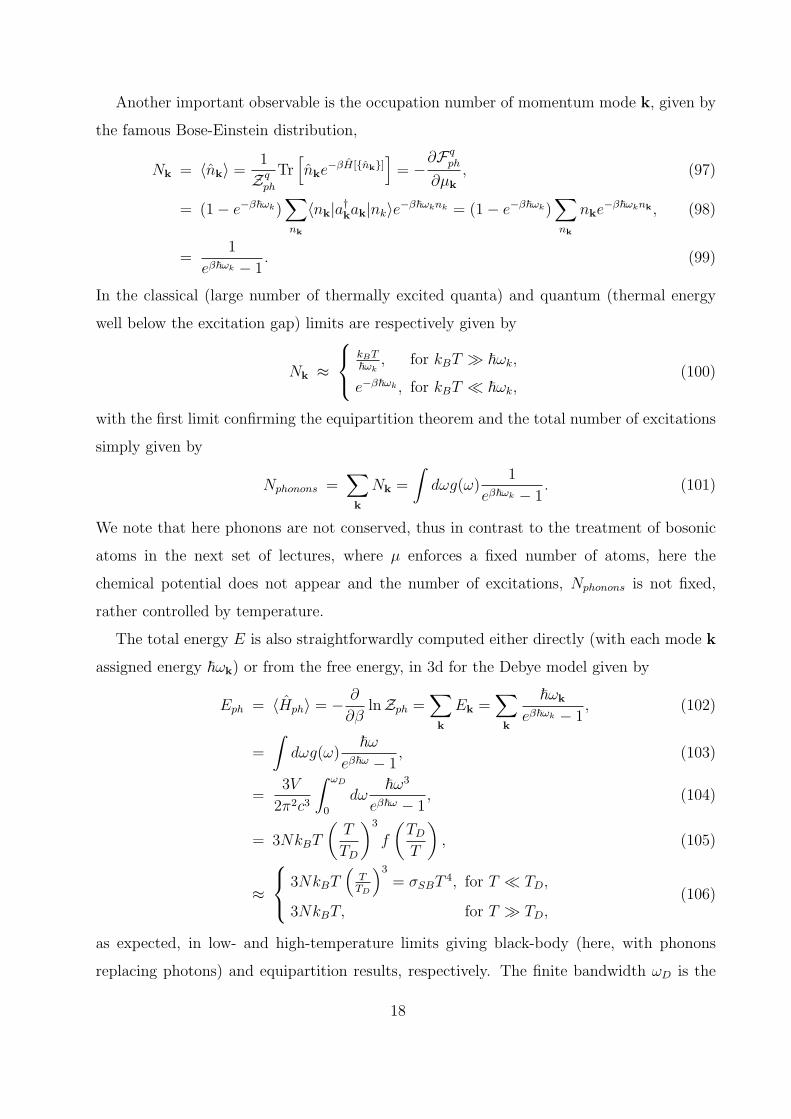
illustrated in Fig.2.

FIG. 2: A dispersion of a one-dimensional monatomic harmonic chain.

In the long-wavelength limit, 1/k a, the dispersion is linear

ω(k) ≈(B

M

)1/2

a|k| ≡ c|k|, (19)

with sound group velocity c =(

BM

)1/2a = ω0a and dispersive group velocity cg(k) = |∂ω/∂k|

away from k = 0. This vanishing dispersion property is quite general and is a reflection of

the underlying translational symmetry that is spontaneous “broken” by crystallization, with

the phonon uR the corresponding Goldstone mode.[1–3]

In building up to quantum field theory of solid state systems, it is more convenient to

diagonalize the Hamiltonian directly (rather than the equation of motion). Expressing H in

Eq.(12) in terms of the normal modes uk, we find

H1d =N∑

n=1

P 2n

2M+Mω2

0

2N

N∑n=1

∑p1,p2

up1up2ei2πn(p1+p2)/N

(ei2πp1/N − 1

) (ei2πp2/N − 1

)(20)

5

Applying a simple identity

N∑n=1

ei2πn(p1+p2)/N = Nδp1+p2,0 (21)

the Hamiltonian reduces to

H1d =N∑

n=1

1

2MP 2

n +

N/2∑p=−N/2

1

2Mω2

p|up|2, (22)

=

π/a∑k=−π/a

[1

2M|Pk|2 +

1

2Mω2

k|uk|2], (23)

=

π/a∑k=−π/a

[1

2MP †

k Pk +1

2Mω2

ku†kuk

], (24)

with

ωk = 2ω0| sin(ka/2)|.

Although to decouple the Hamiltonian, it is sufficient to just Fourier transform the dis-

placement un → uk, as we did in the second form above, we are forced to also trans-

form the momentum Pn → Pk, in order to maintain the canonical commutation relation,

[uk1 , Pk2 ] = i~δk1,−k2 , giving

[uk, P†k ] = i~,

where because the fields in coordinate space are real, P †k = P−k, as can be straightforwardly

verified.

Thus Fourier representation indeed diagonalizes the Hamiltonian, decoupling it into N

independent harmonic oscillators with frequency ωk identical to that we found from the

equation of motion.

For homework we will study a chain with two-atom basis that requires a diaogonalization

of a 2× 2 matrix even after Fourier transform and leads to two, optical and acoustic bands.

(also see Solyom Sec. 11.2)

2. Normal modes quantization

It is now straightforward to quantize oscillations of the crystal lattice by simply treating

it as a sum of N independent quantum harmonic oscillators. The answer can be written

6

automatically, given that H1d =∑

k Hk is a sum of independent harmonic oscillator Hamil-

tonians, given in the Fock occupation nk basis for each k by

Hk|nk〉 = Enk|nk〉,

where |nk〉 =∏

k |nk〉, with the many-body spectrum

E(nk) =∑

k

Enk=∑

k

~ωk(nk + 1/2).

For completeness we diagonalize the crystal Hamiltonian by expressing it in terms of

creation and annihilation operators for each Hk following standard procedure. Namely, we

express uk and Pk in terms of ak and a†k, with latter satisfying bosonic commutation relation

[ak, a†k] = 1 and ak|nk〉 =

√nk|nk − 1〉, a†k|nk〉 =

√nk + 1|nk + 1〉.

Generically the normal mode k harmonic Hamiltonian Hk is given by

Hk =1

2αkP

†k Pk +

1

2βku

†kuk, (25)

=1

2~√αkβk

[1

~2

√~2αk

βk

P †k Pk +

√βk

~2αk

u†kuk

], (26)

≡ ~ωk

(a†kak + 1/2

), (27)

where we identified the natural frequency and a quantum oscillator length

ωk =√αkβk, u0k =

(~2αk

βk

)1/4

(28)

and introduced creation and annihilation operators in terms of dimensionless displacement

uk ≡ uk/u0 and momentum Pk ≡ Pk/(~/u0k)

ak =

√1

2(uk + iPk), a†k =

√1

2(u†k − iP †

k ), (29)

(30)

obeying canonical commutation relation [ak, a†k] = 1. Equivalently,

uk = u0k

√1

2(ak + a†−k), Pk = −i ~

u0k

√1

2(ak − a†−k). (31)

In real space the field operators are then given by

uR =

√1

2N

k=π/a∑k=−π/a

u0k(akeikR + a†ke

−ikR), PR = −i√

1

2N

k=π/a∑k=−π/a

~u0k

(akeikR − a†ke

−ikR). (32)

7

C. Continuum elastic formulation

For a many applications, it is convenient to take a continuum limit of the above formu-

lation, valid for acoustic mode in the limit of small k, i.e., ka 1. In this limit, the general

lattice form (7) simplifies by approximating phonon differences by a gradient expansion

u(Rm)− u(Rn) ≈ ((Rm −Rn) ·∇r)u(r)|r=Rn ,

giving

Uel[u(r)] ≈ 1

2

∫drCαβ,γδ uαβuγδ (33)

where (going to continuum with unit cell v)

Cαβ,γδ =1

2v

∑Rm

(Rm −Rn)αUs,tβδ (|Rm −Rn|)(Rm −Rn)γ (34)

is the elastic structure constant, whose detailed form is determined by crystal symmetry,

but generically by construction symmetric on the first two and last two indices, and under

interchange of the pairs of indices

Cαβ,γδ = Cβα,γδ = Cαβ,δγ = Cγδ,αβ,

and

uαβ =1

2(∂αuβ + ∂βuα + ∂αu · ∂βu), (35)

≈ 1

2(∂αuβ + ∂βuα) ≡ εαβ (36)

is a symmetric strain tensor, where in the second line we approximated it by its harmonic

form, εαβ. Strain’s general structure is gauranteed by the underlying lattice rotational in-

variance, demanding that at harmonic level the elastic energy cannot dependent on the

antisymmetric part 12(∂αuβ − ∂βuα) that corresponds to lattice rotation. The diagonal ele-

ments uxx, uyy, uzz represent bond length change, while the off-diagonal elements uxy, uyz, uxz

correspond to shear. As a generalization of Hooke’s law the elastic structure constant relates

strain to stress

σαβ = Cαβ,γδ uγδ.

8

1. Elasticity in different crystal symmetries

In three dimensions there are 6 independent components of the strain tensor, ε1 =

uxx, ε2 = uyy, ε3 = uzz, ε4 = 2uyz, ε5 = 2uzx, ε6 = 2uxy with the elastic energy density

given by

Uel ≈1

2ci,jεiεj, (37)

For triclinic crystals this leads to 6 × 7/2 = 21 elastic components. This number gets

significantly reduced down to 13 components in a monoclinic crystal system, by invariance

x → −x, y → −y, z → z forbidding odd appearance of ε4 and ε5. In the orthorhombic

crystal the additional 1800 rotation about each of the three axes reduces the count down

to 9 elastic constants by forbidding odd occurence of ε6 and ε4. In tetragonal crystals, 900

rotations around z-axis, x → y, y → −x, z → z reduces the number of elastic constants

down to 6, with the elastic energy density

U tetrael =

1

2c11(u

2xx + u2

yy) +1

2c33u

2zz + c12uxxuyy + c13(uxxuzz + uyyuzz) + 2c44(u

2xz + u2

yz) + 2c44u2xy.

(38)

Adding 900 rotations about x- and y-axes in a cubic crystal reduces the energy density to

U cubicel =

1

2c11(u

2xx + u2

yy + u2zz) + c12(uxxuyy + uxxuzz + uyyuzz) + 2c44(u

2xy + u2

xz + u2yz). (39)

2. Elasticity of “isotropic” solid

In the case of an isotropic (noncrystalline) solid, the elasticity is characterized by only

two elastic constants traditionally called the Lame’ constants, µ and λ, with

Cαβ,γδ = λδαβδγδ + µ(δαγδβδ + δαδδβγ).

In this notation the the shear modulus G = µ, the bulk modulus B = λ+ 2µ/3, the inverse

of the compressibility κ, Poisson ratio ν = λ2(µ+λ)

, Young’s modulus E = µ(2µ+3λ)µ+λ

, and the

elastic energy density reduces to

U isoel = µuαβuαβ +

1

2λuααuββ, (40)

9

expressed in terms of two scalars, Tr[u] and Tr[u2]. The corresponding stress is given by

σαβ = λδαβuγγ + 2µuαβ.

For further analysis it is important to express this elastic energy in terms of the phonon

displacement degrees of freedom, u(r) and then decouple it through normal modes analysis,

that corresponds to Fourier transformation. To this end we use (36) inside (40), finding

U isoel =

1

2

∫r

uα(r)[µ(−∇2)P T

αβ + (2µ+ λ)(−∇2)PLαβ

]uβ(r), (41)

=1

2

∫d3k

(2π)3uα(−k)

[µk2P T

αβ(k) + (2µ+ λ)k2PLαβ(k)

]uβ(k), (42)

≡ 1

2

∫d3k

(2π)3uα(−k)Dαβ(k)uβ(k), (43)

where we utilized normal modes u(k)

u(r) =

∫d3k

(2π)3u(k)eik·r (44)

decomposition to decouple the Hamiltonian, and defined transverse and longitudinal projec-

tion operators, transverse and along k, respectively

P Tαβ(k) = δαβ −

kαkβ

k2, PL

αβ(k) =kαkβ

k2. (45)

Because the projection operators are independent, the inverse of the dynamic matrix Dαβ(k)

(that we will need for study of thermodynamics and correlation functions) is easily obtained

D−1αβ (k) =

1

µk2P T

αβ(k) +1

(2µ+ λ)k2PL

αβ(k), (46)

as can be straightforwardly verified using P TαγP

Tγβ = P T

αβ, PLαγP

Lγβ = PL

αβ, P TαγP

Lγβ = 0.

Interestingly, a two-dimensional hexagonal lattice is also characterized by such isotropic

elasticity, despite being a crystal, with only higher order nonlinear elastic terms distinguish-

ing it from a truly isotropic, amorphous solid.

A related but more general observation that we will use over and over in converting a

Hamiltonian from real-space φ(r) to Fourier φ(k) degrees of freedom is:

H =1

2

∫ddrddr′φ(r)Γ(r− r′)φ(r′),

=1

2

∫ddk

(2π)dφ(−k)Γ(k)φ(k), (47)

that is straightforwardly established by Fourier transformation.

Having established the field theory of elastic degrees of freedom, we now turn to the com-

putation of variety of physical properties, such as thermodynamics and correlation functions.

10

II. THERMODYNAMICS

To analyze the thermodynamics it is convenient to work in canonical ensemble, where

much can be extracted from the partition function or corresponding correlation function:

Zclassicalphonons =

∫[dP][du]e−βH[P,u], (48)

〈...〉 =1

Zclassicalphonons

∫[dP][du]...e−βH[P,u], (49)

Zquantumphonons = Tr

[e−βH[P,u]

], (50)

〈...〉 =1

Zquantumphonons

Tr[...e−βH[P,u]

], (51)

where as usual β = 1/(kBT ), the normalization by 2π~ per degree of freedom is implicitly,

and in the quantum case the degrees of freedom P, u are operators with the Trace taken

over any complete set of states in the Hilbert space.

Before turning to the calculation of thermodynamics, we pause to develop the very im-

portant theoretical tool of Gaussian integrals, that we will utilize over and over again here

and throughout the course.

A. Gaussian integrals

Given that the harmonic oscillator is a work-horse of theoretical physics, it is not suprising

that Gaussian integrals are the key tool of theoretical physics. It is certainly clear in the com-

putation of the partition function of the classical harmonic oscillator as it involves Gaussian

integration over fields P and u. However, as we will see, utilizing Feynman’s path-integral

formulation of quantum mechanics, Gaussian integrals are also central for computation in

quantum statistical mechanics and more generally in quantum field theory.

11

1. one-dimension

Let us start out slowly with standard scalar Gaussian integrals

Z0(a) =

∫ ∞

−∞dxe−

12ax2

=

√2π

a, (52)

Z1(a) =

∫ ∞

−∞dxx2e−

12ax2

= −2∂

∂aZ0(a) =

1

a

√2π

a=

1

aZ0, (53)

Zn(a) =

∫ ∞

−∞dxx2ne−

12ax2

=(2n− 1)!!

anZ0, (54)

that can be deduced from dimensional analysis, relation to the first basic integral Z0(a)

(that can in turn be computed by a standard trick of squaring it and integrating in polar

coordinates) or another generating function and Γ-functions

Z(a, h) =

∫ ∞

−∞dxe−

12ax2+hx =

∫ ∞

−∞dxe−

12a(x−h/a)2e

12h2/a = Z0(a)e

12h2/a, (55)

=∑n=0

h2n

(2n)!Zn(a). (56)

Quite clearly, odd powers of x vanish by symmetry.

A useful generalization of above Gaussian integral calculus is to integrals over complex

numbers. Namely, from above we have

I0(a) =

∫ ∞

−∞

dxdy

πe−a(x2+y2) =

1

a=

∫dzdz

2πie−azz, (57)

where in above we treat z, z as independent complex fields and the normalization is deter-

mined by the Jacobian of the transformation from x, y pair. This integral will be envaluable

for path integral quantization and analysis of bosonic systems described by complex fields,

ψ, ψ.

2. d-dimensions

This calculus can be straightforwardly generalized to multi-variable Gaussian integrals

characterized by an N ×N matrix (A)ij,

Z0(A) =

∫ ∞

−∞[dx]e−

12xT ·A·x =

N∏i=1

√2π

ai

=

√(2π)N

detA, (58)

Zij1 (A) =

∫ ∞

−∞[dx]xixje

− 12xT ·A·x = Z0A

−1ij , (59)

Z(A,h) =

∫ ∞

−∞[dx]e−

12xT ·A·x+hT ·x = Z0(A)e

12hT ·A−1·h, (60)

12

computed by diagonalizing the symmetric matrix A and thereby decoupling the N -

dimensional integral into a product of N independent scalar Gaussian integrals (54), each

characterized by eigenvalue ai.

As a corollary of these Gaussian integral identities we have two more very important

results, namely, that for a Gaussian random variable x obeying Gaussian statistics, with

variance A−1ij , we have

〈xixj〉 ≡ Gij =1

Z0

∫ ∞

−∞[dx]xixje

− 12xT ·A·x = A−1

ij , (61)

〈ehT ·x〉 = e12〈(hT ·x)2〉 = e

12hT ·G·h, (62)

with second identity the relative of the Wick’s theorem, which will be extremely important

for computation of x-ray and neutron scattering structure function.

3. discrete vs continuum description

Throughout our lectures we will go back and forth between discrete and continuum de-

scription of the degrees of freedom. In all calculations, even when done in the continuum

limit, it is quite important to keep in mind the discrete and therefore finite nature of the

degrees of freedom, with the continuum description being simply an efficient pnemonic for

the underlying lattice model. This guarantees that no true short-scale (ultra-violet, uv)

divergences actually ever arise, cutoff by the physical lattice structure always present in any

condensed matter system.

Given that a volume of a unit cell is v and reciprocal space is quantized in units of 2π/L,

the relations between sums and integrals in real and reciprocal spaces are given by∑R

. . . =1

v

∫ddr . . . , (63)

∑k

. . . = Ld

∫ddk

(2π)d. . . . (64)

13

Also, we note the relation between the Kronecker δ and δ-function identities,

N∑R

eik·R = Nδk,0, (65)

N∑R

veik·R = vNδk,0, (66)∫ddreik·r = V δk,0 =

(2π)d

(2π/L)dδk,0 = (2π)dδd(k), (67)

where V = vN .

4. density of states

There will be many instances where our result is represented as a sum over the normal

eigenmodes k. If the summand is only a function the normal-mode frequency ωk (as will

often be the case) it is convenient to replace the sum over k by an integral over ω, with the

Jacobian of this transformation being the density of states g(ω), defined according to:

F =∑k,α

f(ωk) =

∫dω

(∑k,α

δ(ω − ωk)

)f(ω), (68)

=

∫dωg(ω)f(ω), (69)

where the number of states k per interval dω around ω is given by density of states

g(ω) = d∑k

δ(ω − ωk) = dLd

∫ddk

(2π)dδ(ω − ωk), (70)

where there are d polarizations that we have taken to be degenerate. We note that sometimes

g(ω) is defined without the volume factor Ld, corresponding to density of states per unit of

volume. Also, by construction, g(ω) satisfies the sum rule∫dωg(ω) = N .

The limit on large k is given by G set by the first BZ, corresponding to uv cutoff by the

lattice spacing in Rn. There is also infrared cutoff set by the system size, L or equivalently

in momentum space by discreteness of k = 2πLp.

There are two canonical models of phonons, the Debye model with ωk = ck and the Ein-

stein model with ωk = ω0. The density of states for these “toy”models are straightforwardly

14

computed to be

gDebye(ω) = dLd

∫ddk

(2π)dδ(ω − ck), (71)

= Ld dSd

(2π)dcdωd−1, for 0 < ω < ωDebye (72)

gEinstein(ω) = dLd

∫ddk

(2π)dδ(ω − ωo), (73)

= dNδ(ω − ωo), (74)

where Sd = 2πd/2/Γ(d/2) is a surface area of a d-dimensional sphere and ωD is defined by

dN =∫ ωD

0dωgDebye(ω).

B. Phonon thermodynamics

Armed with these tools, we now apply them to compute the free energy of a crystal lattice

associated with atomic vibrations.

1. classical treatment

In the classical limit, we compute the partition function Zcph in (48) by integrating over

functional phase space of momentum and phonon displacement fields, P,u using (60). In

the classical limit, these are decoupled and the integral over the momentum field just gives

an overall 3N -th power of the thermal deBroglie wavelength, λT =√

2π~2

mkBT. The remaining

phonon integral is also straightforwardly done in terms of the normal phonon modes, giving

Zcph =

∫[dPk]e

−βRk

|Pk|2

2M

∫[duk]e

−βRk

12uT−k·Dk·uk , (75)

=∏k

(M

~2

)3/2(kBT )3

(detDk)1/2, (76)

The resulting Helmholtz free energy F = −kBT lnZ is then given by

F cph =

1

2kBT

∑k

ln (detDk) + const. (77)

where the const. part comes from the momentum degrees of freedom, unimportant to us

here, particularly because (due to lack of phase space discreteness) an additive constant to

the free energy (and entropy) is not very meaningful in classical statistical mechanics.

15

The energy is also easily computed by averaging the classical Hamiltonian and utilizing

the Gaussian integrals in (60). This directly leads to equipartition for the average energy

and heat capacity

E = 3NkBT, CV =∂E

∂T

∣∣∣∣V

= 3NkB. (78)

The phonon correlation function is also directly given by the Gaussian integrals above,

〈uαku

βk′〉 = kBTD

−1αβ (k)(2π)3δ3(k + k′), (79)

and in particular for “isotropic” solid is given by (46). In coordinate space it is given Fourier

transform, (44)

〈uαru

βr′〉 = kBT

∫d3k

(2π)3D−1

αβ (k)eik·(r−r′), (80)

a result that we will use extensively.

2. quantum treatment

We compute quantum thermodynamics utilizing canonical quantization, generalizing the

1d elastic chain treatement of Sec.(I B) to higher dimensions here. Normal modes decompo-

sition (with eigenvectors ei)

uR =

√1

N

∑k∈1BZ

ukeik·R, (81)

=

√1

2N

∑i,k∈1BZ

u0kiei(ak,ieik·R + a†k,ie

−ik·R), (82)

PR =

√1

N

∑k∈1BZ

Pkeik·R, (83)

= −i√

1

2N

∑i,k∈1BZ

~u0ki

ei(ak,ieik·R − a†k,ie

−ik·R). (84)

gives a harmonic phonon Hamiltonian

Hph =∑

k∈1BZ

[1

2MP†

k · Pk +1

2u†

k ·Dk · uk

], (85)

=∑

i,k∈1BZ

[1

2MP †

k,iPk,i +1

2Mω2

k,iu†k,iuk,i

], (86)

≡∑

k∈1BZ

~ωk,i

(a†k,iak,i + 1/2

), (87)

16

where we identified the natural frequency ωk,i =√dk,i/M with eigenvalues dk,i of the dy-

namical matrix Dk and a quantum oscillator length

u0ki =

√~

Mωk,i

, (88)

and introduced creation and annihilation operators in terms of dimensionless displacement

uk,i ≡ uk,i/u0ki and momentum Pk,i ≡ Pk,i/(~/u0ki)

ak,i =

√1

2(uk,i + iPk,i), a†k,i =

√1

2(u†k,i − iP †

k,i), (89)

obeying canonical commutation relation [ak,i, a†k′,j] = δijδk,k′ .

To obtain the dynamics we recall that the time dependence of the Heisenberg operators

is given by OH(t) = eiHt/~OH(0)e−iHt/~, or equivalently given by the solution of the Heisen-

berg equation of motion, i~dOH

dt= [OH , H]. Applying this to the creation and annihilation

operators, we obtain

ak(t) = ake−iωkt, a†k(t) = a†ke

iωkt. (90)

The trace in (51) can be computed in the occupation basis |nk,i〉, (eigenstates of the

Hamiltonian, (87), and is given by (summing the geometric series)

Zqph =

∑nk

〈nk|e−βH[a†k,ak]|nk〉, (91)

=∏k

∞∑nk=0

e−β~ωk(nk+1/2), (92)

=∏k

e−12β~ωk

1− e−β~ωk, (93)

and the associated free energy, Fph = −kBT lnZph

F qph = kBT

∑k

ln(1− e−β~ωk

)+∑k

1

2~ωk, (94)

= kBT

∫dωg(ω) ln

(1− e−β~ω

)+

∫dωg(ω)

1

2~ω, (95)

(96)

with the last term the zero-point energy. In above, for simplicity of notation we implic-

itly incorporated the eigenvector index i into the mode label k and will restore it later as

necessary.

17

Another important observable is the occupation number of momentum mode k, given by

the famous Bose-Einstein distribution,

Nk = 〈nk〉 =1

Zqph

Tr[nke

−βH[nk]]

= −∂F q

ph

∂µk

, (97)

= (1− e−β~ωk)∑nk

〈nk|a†kak|nk〉e−β~ωknk = (1− e−β~ωk)∑nk

nke−β~ωknk , (98)

=1

eβ~ωk − 1. (99)

In the classical (large number of thermally excited quanta) and quantum (thermal energy

well below the excitation gap) limits are respectively given by

Nk ≈

kBT~ωk

, for kBT ~ωk,

e−β~ωk , for kBT ~ωk,(100)

with the first limit confirming the equipartition theorem and the total number of excitations

simply given by

Nphonons =∑k

Nk =

∫dωg(ω)

1

eβ~ωk − 1. (101)

We note that here phonons are not conserved, thus in contrast to the treatment of bosonic

atoms in the next set of lectures, where µ enforces a fixed number of atoms, here the

chemical potential does not appear and the number of excitations, Nphonons is not fixed,

rather controlled by temperature.

The total energy E is also straightforwardly computed either directly (with each mode k

assigned energy ~ωk) or from the free energy, in 3d for the Debye model given by

Eph = 〈Hph〉 = − ∂

∂βlnZph =

∑k

Ek =∑k

~ωk

eβ~ωk − 1, (102)

=

∫dωg(ω)

~ωeβ~ω − 1

, (103)

=3V

2π2c3

∫ ωD

0

dω~ω3

eβ~ω − 1, (104)

= 3NkBT

(T

TD

)3

f

(TD

T

), (105)

≈

3NkBT(

TTD

)3

= σSBT4, for T TD,

3NkBT, for T TD,(106)

as expected, in low- and high-temperature limits giving black-body (here, with phonons

replacing photons) and equipartition results, respectively. The finite bandwidth ωD is the

18

crucial distinquishing feature, here, that is infinite in the case of photons. In above we

defined the Debye temperature by the corresponding frequency, kBTD ≡ ~ωD and used the

low- and low-temperature limits of scaling function f(TD/T ) given by

f(x) = 3

∫ x

0

dωω3

eω − 1, (107)

≈

1, for x 1,

x3, for x 1,(108)

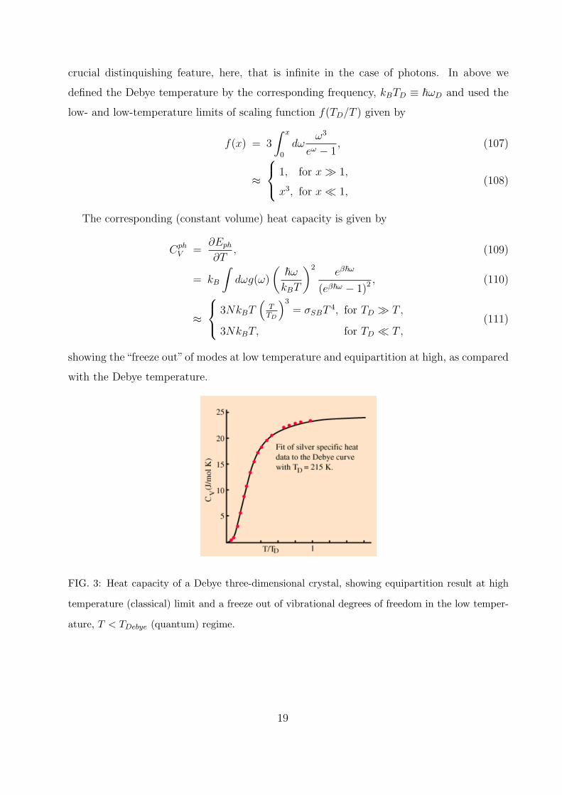
The corresponding (constant volume) heat capacity is given by

CphV =

∂Eph

∂T, (109)

= kB

∫dωg(ω)

(~ωkBT

)2eβ~ω

(eβ~ω − 1)2 , (110)

≈

3NkBT(

TTD

)3

= σSBT4, for TD T ,

3NkBT, for TD T ,(111)

showing the“freeze out”of modes at low temperature and equipartition at high, as compared

with the Debye temperature.

FIG. 3: Heat capacity of a Debye three-dimensional crystal, showing equipartition result at high

temperature (classical) limit and a freeze out of vibrational degrees of freedom in the low temper-

ature, T < TDebye (quantum) regime.

19

III. CORRELATION FUNCTIONS AND X-RAY SCATTERING

A. Phonon correlation function

The phonon correlation function 〈uαRu

βR′〉 can now be computed, utilizing our normal

mode decomposition and quantization, (84) above and giving the quantum counter part of

the classical result in (80).

〈uαRu

βR′〉 =

1

N

∑k∈1BZ

〈u†k,αuk,β〉eik(·R−R′), (112)

=1

2N

∑i,j,k,k′∈1BZ

u0kiu0kj eαi e

βj 〈(ak,i + a†−k,i)(ak′,j + a†−k′,j)〉e

ik·R+ik′·R′(113)

=1

2N

∑i,j,k∈1BZ

u0kiu0kj eαi e

βj 〈(ak,ia

†k,j + a†−k,ia−k,j〉eik·(R−·R′), (114)

=1

2N

∑i,j,k∈1BZ

u0kiu0kj eαi e

βj (2Nk,i + 1)eik·(R−·R′), (115)

=1

2N

∑i,k∈1BZ

u0kiu0kieαi e

βi coth(

~ωk,i

2kBT)eik·(R−·R′), (116)

=1

2N

∑i,k∈1BZ

~Mωk,i

eαi e

βi coth(

~ωk,i

2kBT)eik·(R−·R′), (117)

≈ 1

N

∑i,k∈1BZ

kBT

Mω2k,ieα

i eβi e

ik·(R−·R′), for ~ωk,i 2kBT , classical,

12N

~Mωk,i

eαi e

βi e

ik·(R−·R′), for ~ωk,i 2kBT , quantum,(118)

where we used u−k = u†k, lattice translational invariance, and finite T normal modes occu-

pation Nk, (99).

For the scalar product this simplies to

〈uR · uR′〉 =1

2N

∑i,k∈1BZ

~Mωk,i

coth(~ωk,i

2kBT)eik·(R−·R′) (119)

where we used orthonormality of the eigenvectors ei · ei = 1.

B. Structure function

1. scattering

The atomic structure of liquids and solids can be probed using a variety of scattering

techniques such as x-ray and neutron scattering. Atoms introduce a scattering potential

20

V (r) =∑N

i=1 Vatom(r−Ri), that is proportional to their density distribution. X-rays photons

interact with electron density in the outer atomic shell, with the scattering potential with

Vatom(r−Ri) ∝ ρe(r−Ri), where ρe(r) is the charge distribution on atom i at Ri. In constrast

neutrons interact with the nearly point-like nuclei with the potential well-represented by

Vatom(r) = 2π~2

mnasδ

3(r − Ri), where as single atom scattering length. We are interested in

the probability of the scattering process of an incoming plane wave k into the outgoing plane

wave k′, with a scattering amplitude

〈k′|V (r)|k〉 =1

Nv

∫r

V (r)e−i(k′−k)·r, (120)

=1

N

∑i

e−i(k′−k)·Ri1

v

∫r

Vatom(r)e−i(k′−k)·r, (121)

= V atomq

1

N

∑i

e−iq·Ri = V atomq ρq, (122)

where q = k′ − k is the scattering wavevector (momentum transfer to the photon) and

V atomq is the Fourier transform of the single atom potential, determining the form factor at

high momenta. It is the second factor that is of most interest to us as it determines the

distribution of centers of atomic positions and is the Fourier transform ρq of the atomic

density of point atoms ρ(r) =∑N

i δ3(r−Ri) at a scattering wavevector q.

The diffraction scattering intensity is characterized by the differential cross-section that

is derived using the Fermi’s Golden rule and is given by

dσ

dΩ= N |V atom

q |2S(q), (123)

where

S(q) =1

N

∑i,j

〈e−iq·(Ri−Rj)〉, (124)

= 〈ρ−qρq〉 (125)

is the static structure function, with correlations computed at equal times. In above we

recognized the fact that in principle Ri are quantum, thermally fluctuating variables and

therefore need to be averaged over to relate the result to the measured diffraction signal. A

generalization of this central quantity to unequal time correlator of ρq(t) = 1√N

∑i e

−iq·Ri(t)

gives the dynamic structure function

S(q, t) =1

N

∑i,j

〈e−iq·(Ri(t)−Rj(0))〉,

21

that is measured in elastic scattering, where in addition to momentum q, the energy ~ω

is also transferred between the probing particle (e.g., x-ray photon or a neutron) and the

atomic system.

The structure function is useful for characterization of density distribution whether the

material is a fluid or a solid. However, here will focus on a crystalline solid, in which

Ri = Rn + uRn with the fluctuating nature of atomic vibrations encoded through the

phonons uR degrees of freedom, whose dynamics is characterized by a elastic Hamiltonian

discussed in previous sections.

We first note that for small fluctuations (heavy ions at low temperature) we can approxi-

mate the structure fuction by neglecting the phonon fluctuatins, i.e., taking uR = 0. In this

case we find

S(q) =1

N

∑Rn,Rm

e−iq·(Rn−Rm), (126)

=1

N

∑Rn

∑Rn−Rm

e−iq·(Rn−Rm), (127)

=∑Gp

Nδq,Gp = (2π)3v∑Gp

δ3(q−Gp), (128)

a crucial result of lattice Bragg (δ-function) peaks appearing at the reciprocal lattice points

Gp (defined by eiGp·Rn = 1), characterizing the perfect a crystalline order. It is this key

property that makes scattering such an effective tool for analyzing the crystal structure

and deviation from it. The latter comes from lattice defects and fluctuations that are

incorporated into phonons uR, to which we now turn.

2. scattering with phonon fluctuations

To go beyond the above idealized approximation we now include phonons in (125) in the

structure function

S(q, t) =1

N

∑R,R′

e−iq·(R−R′)〈e−iq·uR(t)eiq·uR′ (0)〉, (129)

where uR is a quantum field and the average is over both its quantum and thermal fluctua-

tions. In above we returned to the original definition of the structure function as a two-point

correlator of a Fourier transformed density ρq, and avoided combining the noncommuting

phonon operators in the exponential.

22

A very useful identity, valid for quadratic (Gaussian) operator fields is given by

〈eAeB〉 = e12〈A2〉+ 1

2〈B2〉+〈AB〉, (130)

that can be derived by using Baker-Hausdorff formula (valid for operators whose commutator

is a c-number)

eAeB = eA+Be12[A,B] (131)

together with a formula

〈eφ〉 = e12〈φ2〉,

that we have derived for classical harmonic (Gaussian) fields using Gaussian integrals, but

can also be shown to hold for quantum harmonic fields using path-integral formulation.

Taking A = −iq · uR(t), B = iq · uR′(0), and utilizing identity (130), we obtain for the

dynamic structure function

S(q, t) =1

N

∑R,R′

e−iq·(R−R′)e−CR−R′ (t), (132)

where

CR−R′(t) = 〈(q · uR(t))2〉 − 〈(q · uR(t))(q · uR′(0))〉, (133)

=1

2N

∑i,k∈1BZ

|u0ki|2(q · ek,i)2[〈ak,ia

†k,i〉(1− eik·(R−R′)−iωkt

)+〈a†k,iak,i〉

(1− e−ik·(R−R′)+iωkt

)], (134)

=1

2N

∑i,k∈1BZ

~Mωi,k

(q · ek,i)2[(Nk,i + 1)

(1− eik·(R−R′)−iωkt

)+Nk,i

(1− e−ik·(R−R′)+iωkt

)],

=1

2N

∑i,k∈1BZ

~Mωi,k

(q · ek,i)2 coth(

~ωk,i

2kBT)(1− eik·(R−R′)−iωkt

). (135)

we took advantage of the translational invariance of the connected phonon correlation func-

tion, invariance of the summand under k → −k, and used the time dependence of the normal

modes based on the Heisenberg equation of motion (90) that gives

uR(t) =

√1

2N

∑i,k∈1BZ

u0kiek,i(ak,ieik·R−iωkt + a†k,ie

−ik·R+iωkt). (136)

For isotropic crystal, eαi e

βi (no sum over i) gives PL,T

αβ (k) for i = L, T , respectively.

23

Time Fourier transform of S(q, t) gives the dynamic structure S(q, ω) measured in elastic

scattering with energy transfer of ~ω.

Specializing to the equal time correlator t = 0, gives the static function, S(q), with

exponent CR−R′(t = 0). At large spatial separations, the oscillating averages out and the

correlator asymptotes to a constant W given by

CR−R′(0) = W, |R−R′| a, (137)

=1

N

∑i,k∈1BZ

~2Mωi,k

(q · ek,i)2 coth(

~ωk,i

2kBT), (138)

= ad

∫ddk

(2π)d

∑i=L,T

~2Mωi,k

qαqβPiαβ coth(

~ωk,i

2kBT), (139)

= q2add

∫ddk

(2π)d

~2Mcsk

coth(~csk2kBT

), (140)

where we went over to the continuum limit and for simplicity specialized to an isotropic

lattice and then taken λ = −µ so that longitudinal transverse speeds of sound are degenerate,

cL = cT .

In the quantum limit, ~ωk kBT (note that for acoustic phonons where ωk vanishes as

k → 0, this requires ultra-low T → 0), the coth( ~csk2kBT

) factor is 1 and for d > 1, W reduces

to

W ≈ q2 dCd

d− 1

~2Mcsa−1

,

= q2 ~MωD

dCd

2(d− 1)= cdq

2u20D (141)

where cd ≡ dCd

2(d−1), u2

0D ≡ ~MωD

is the quantum oscillator length at the BZ edge scale π/a, we

cutoff the upper limit of the integral by the BZ edge, k = π/a ≡ Λ, and denoted surface area

Sd = 2πd/2/Γ(d/2) of a d-dimensional unit sphere (S2 = π, S3 = 4π) divided by (2π)d by Cd.

Note that for d ≤ 1, the integral diverges in the infrared, i.e., with system size L according to

W (L) ∼ L(1−d) (∼ lnL/a, for d = 1), which is a reflection of the Hohenberg-Mermin-Wagner

theorem of the absence of long range order (breaking of continuous symmetry at T = 0 in

one dimension and below.

In the classical limit, ~ωk kBT (note that for this to be true for all of k, this actually

requires the condition on the highest frequency ~ωΛ ≡ ~ωD kBT ) the coth( ~csk2kBT

) ≈

2kBT/(~csk) and for d ≤ 2, W reduces to

W ≈ q2a2 dCd

d− 2

kBT

Mc2s= bDq

2a2 T

TD

, (142)

24

where bD ≡ dCd

d−2. Note that for d ≤ 2, the integral diverges in the infrared, i.e., with

system size L according to W (L) ∼ L(2−d) (∼ lnL/a, for d = 2), which is a reflection of

the Hohenberg-Mermin-Wagner theorem of the absence of long range order (breaking of

continuous symmetry at finite T in two dimensions and below.

Since at T = 0 (finite T > 0) in d > 1 (in d > 2), CR−R′(0) asymptotes to the above

finite value W , the static structure function from (132), S(q) ≡ S(q, t = 0) reduces to

S(q) ≈ 1

N

∑R,R′

e−iq·(R−R′)e−Wq , (143)

=∑Gp

e−WGpNδq,Gp = v∑Gp

e−WGp (2π)3δ3(q−Gp), (144)

retaining perfect Bragg (δ-function) peaks even in the presense of thermal and quantum

phonon fluctuations, that simply reduce it by the so-called Debye-Waller q-dependent Gaus-

sian form factor, e−Wq .

On the other hand for T = 0 (finite T > 0) in d ≤ 1 (in d ≤ 2), CR−R′(0) is a growing

function of |R −R′|, that leads to S(q) that exhibits broadenned, finite width (in critical

dimension d = 1 (d = 2) quasi-Bragg) peaks at Gp’s, demonstrating short-range crystalline

order in these lower dimensions.

Indeed in 2D (crystalline film) evaluating above correlator CR−R′ in the continuum classi-

cal limit, for simplicity specializing to an isotropic crystal with λ = −µ, with linear dispersion

(Debye model) gives

CR−R′ ≈ ηq(T ) ln (|R−R′|/a) , (145)

where the exponent ηq(T ) is given by

ηq(T ) = q2a2 T

πTD

= q2kBT

πµ, (146)

with the shear modulus µ carrying units of energy per length-squared in 2D.

Using this inside (132) (with t = 0) together with the Poisson summation formula∑R

e−iq·R =∑G

(2π)dδd(q−G)

to evaluate the sum over R, we find a seminal result[5, 6] that

S(q) ∼∑Gp

1

|q−G|2−ηq. (147)

25

It demonstrates that at finite temperature T , phonon fluctuations in a 2D crystal divergently

large and lead to a structure function that no longer exhibits true (δ-function) Bragg peaks,

but instead is characterized by quasi-Bragg power-law peaks, i.e., it exhibits translatonal

quasi-long-range order, with G spanning a lattice reciprocal to the real-space lattice of R.

IV. MELTING

A detailed theory of melting of a crystal can be quite elaborate, particularly because

this transition is generically first-order and so depends on the microscopic details.[4] Two

dimensional crystals melt via a (infinitely) continuous transition according to a beautiful

and quite elaborate Kosterlitz-Thouless-Halperin-Nelson-Young theory[5–7] closely related

to the Kosterlitz-Thouless Normal-Superfluid transition of 2D films.

However, one can estimate the melting temperature, Tm through a very simple criterion

due to Lindemann named after him[8]. It very reasonably states that the melting of a crystal

takes place when its root-mean phonon fluctuation become of order inter-atomic spacing a,

namely

urms(Tm) ≈ cLa,

where cL is a Lindemann phenomenological contant typically taken to be 0.1 but can very

significantly between different crystals. Given the phenomenological nature of the Linde-

mann criterion, it is most useful for qualitative rather than quantitative estimates of the

melting temperature Tm.

Using the classical, high-temperature limit result

u2rms(T ) = 3

kBT

2Mc2sa2 ≈ kBT

~ωD

a2, (148)

derived on the homework, inside the Lindemann criterion we obtain,

Tm ≈ cL~ωD

kB

= cLTD.

Repeating the calculation of root-mean-squared fluctuations in a 2d crystal (as found on

the homework) gives

u2rms,2d ≈

kBT

~ωD

a2 ln(L/a),

fluctuations that diverge logarithmically with the growing system size L/a → ∞. This

divergence is a manifestation of the so-called Hohenberg-Mermin-Wagner theorem, that in

26

particle physics is referred to as the Coleman’s theorem. It has profound implications of

the absence of true long-range crystalline order in 2d crystals, that translates into absence

of δ-function Bragg peaks in its static structure function S(q), in contrast to that of a 3d

crystal, that well-described by (128).

V. NONLINEAR ELASTICITY

Although so far we have treated the elasticity within harmonic approximation, real crys-

tals exhibit nonlinear elasticity, that is essential to include to capture a number of physical

phenomena.

Recall that the elastic crystal energy to quadratic order in the elastic strain uαβ is given

by

Hel[u(r)] =1

2

∫ddrCαβ,γδ uαβuγδ. (149)

Translational and rotational invariances of the underlying liquid from which a crystal spota-

neously emerges guarantee that the strain is a symmetric tensor of the gradients of the

phonon displacements u(r). While the above elastic energy is quadratic in uαβ, the strain

tensor itself is a nonlinear function of the phonon field uα,

uαβ =1

2(∂αR · ∂βR− δαβ), (150)

=1

2(∂αuβ + ∂βuα + ∂αu · ∂βu), (151)

(152)

where in the first line we used the fact that the strain is the difference between the distortion-

induced metric gαβ and the flat metric δαβ and expressed the position of an atom r that has

been moved to R(r) = r + u(r) in a deformed crystal in terms of the phonon field u(r).

Expressing the elastic Hamiltonian in terms of the phonon fields u, and keeping nonlin-

earities for the case of an isotropic crystal, we find

Hel = µuαβuαβ +1

2λuααuββ, (153)

= µ(εαβ +1

2∂αu · ∂βu)(εαβ +

1

2∂αu · ∂βu) +

λ

2(εαα +

1

2∂αu · ∂αu)2, (154)

= µεαβεαβ +λ

2εααεββ +Hnonlin = H0

el +Hnonlin, (155)

27

where

Hnonlin = µ(∂αuβ)(∂αu · ∂βu) +λ

2(∂αuα)(∂βu · ∂βu)

+µ

4(∂αu · ∂βu)(∂αu · ∂βu) +

λ

8(∂αu · ∂αu)(∂βu · ∂βu), (156)

are the cubic and quartic nonlinearities, and H0el is the harmonic energy density from (43).

For low T and small fluctuations (away from the melting transition or any structural

instabilities), contributions of these nonlinearities will typically be small. Thus they can

be accounted for in physical properties (e.g., the free energy, thermal expansion, structure

function, etc.) by Taylor-expanding the Boltzmann weight (or a quantum evolution operator)

in terms of Hnonlin, averaging over it with the Gaussian weight based on H0el.

As a concrete example, we can consider a computation of a thermal expansion of a crystal.

This is given by the change in the volume V due to fluctuations and distortions, characterized

by metric gαβ = δαβ + 2uαβ

δV = 〈∫ddr(

√detg − 1)〉, (157)

= 〈∫ddr(

√det(1 + 2u)− 1)〉, (158)

≈ 〈∫ddr(

√(1 + 2Tr(u))− 1)〉, (159)

≈∫ddr〈Tr(u)〉, (160)

≈∫ddr(〈∂αuα〉+

1

2〈∂αu · ∂αu〉), (161)

where in general the average is done with the Boltzmann weight, characterized by a quantum

Hamiltonian Hel, above. It can typically be computed perturbatively in Hnonlin. This

involves, for a classical regime a computation of various Gaussian averages of powers of u(r)

and for a quantum case averages over powers of ak, a†k. We will not pursue this further here.

[1] Fundamentals of the Physics of Solids I, Electronic Properties, J. Solyom.

[2] Quantum Field Theory of Many-body Systems, by Xiao-Gang Wen.

[3] Principles of Condensed Matter Physics, by P. M. Chaikin and T. C. Lubensky.

[4] L.D. Landau, Phys. Z. Sowjetunion II, 26 (1937); see also S. Alexander and J. McTague,

Phys. Rev. Lett. 41, 702 (1984).

28

[5] J.M. Kosterlitz and D.J. Thouless, J. Phys. C 6, 1181 (1973); see also, V.L. Berezinskii, Zh.

Eksp. Teor. Fiz. 59, 907 (1970) [Sov. Phys. JETP 32, 493 (1971)]; Zh. Eksp. Teor. Fiz. 61,

1144 (1971) [Sov. Phys. JETP 34, 610 (1972)];

[6] B.I. Halperin and D.R. Nelson, Phys. Rev. Lett. 41, 121 (1978); D.R. Nelson and B.I. Halperin,

Phys. Rev. B 19, 2457 (1979).

[7] A.P. Young, Phys. Rev. B 19, 1855 (1979).

[8] F. A. Lindemann, “The calculation of molecular vibration frequencies”, Physik. Z. 11, 609-612

(1910).

29