Physics 570

Tangent Vectors, Differential Forms, and Tensors

0. Symbols to describe various Vector and Tensor Spaces

1. We first note that Finley uses the (common) useful mathematical notations that R stands

for the set of all real numbers, and then Rn is the set of all “n-tuples” of real numbers, while

C stands for the set of all complex numbers. Then Z denotes the set of all integers, and also

Z+ stands for the set of all non-negative integers.

We use the symbol M to denote a manifold. If the manifold is arbitrary, it may be, for

instance, of dimension n; however, our spacetime is of course a manifold of dimension 4. [For

more details on how a manifold is defined, see the notes on the geometrical views on manifolds,

vectors, differential forms, and tensors.]

We are also interested in various functions, mapping manifolds into the real numbers,

R, and denote the set of all of them by the symbol F , or F(M) if it is necessary to specify

which manifold. We usually are only interested in functions which (at least almost everywhere)

possess arbitrarily many continuous derivatives. We refer to such a mapping as being either

“of class C(∞), or simply as “smooth.”

2. In principle there are two, physically-different kinds of vectors, each of which has their cor-

responding vector space. These are the space of “tangent vectors,” T 1 (or sometimes just

T ), and the space of “differential forms,” Λ1, also called cotangent vectors. Tangent vec-

tors are the usual sort of vectors that one regularly uses in, say, freshman physics; however,

differential forms are really ways to label, and “add,” etc. hypersurfaces (of dimension n − 1

in an n-dimensional manifold, so that ours will usually be 3-surfaces). This is like the usual,

freshman-physics notion of the “normal” to a surface, this time, of course, in a 3-dimensional

space.

An equivalent, but very different sounding characterization of differential forms is as (con-

tinuous) linear maps of tangent vectors into scalars, e.g., R or C. Common mathematical

language is to say that differential forms are dual to tangent vectors; i.e., Λ1 is the dual vector

space to T 1.

Geometrically, one should think of tangent vectors as (locally) tangent to 1-dimensional

curves on M, while differential forms are (locally) tangent to hypersurfaces, i.e., n − 1-

dimensional surfaces. From that point of view, the “action” of a hypersurface on a tangent

vector, i.e., what it does to map that vector into a scalar, is to determine how many times the

one intersects the other, that being the resultant scalar.

Because the spaces we are considering usually have a scalar product, the distinction be-

tween these two kinds becomes blurred a bit since the scalar product can be used to map one

kind into the other kind. That is to say, one may use the metric (tensor) to map tangent

vectors into differential forms, or vice versa. We will discuss this in some detail in section

III.4.b below. Geometrically this is the same as the usual approach where we characterize a

hypersurface by the vector which is normal to it.

3. Proceeding onward to notation for these various geometrical objects, we will generalize the

more familiar use of “arrows” over symbols, long used to denote ordinary, 3-dimensional vec-

tors, by using an “over-tilde” to indicate a tangent vector, and an “under-tilde” to indicate a

differential form:

i.) v denotes a tangent vector defined over (at least) some portion of the (spacetime)

manifold; if we need to specify the particular point at which it is being considered, we

may write v|Pto indicate that we are considering it at the point P on the manifold,

ii.) ω∼ is a differential form over the manifold, with the same notation if we need to specify

it at some particular point, while

iii.) p will continue to be used for the usual 3-dimensional vectors, while the notation

above in (i) is intended for a 4-dimensional vector.

iv.) The action of a differential form on a tangent vector will then be written as α∼(v) ∈ R.

4. In any vector space, vectors are often described by giving their (scalar) components with

2

respect to some choice of basis. Our most common spaces of interest will be 4-dimensional;

therefore, most examples will come from there.

a. Finley uses the standard symbols e1, e2, e3, e4 ∈ T 1 to denote an arbitrary basis for a

space of tangent vectors; more compactly, we often write eµ4µ=1, or just eµ41, to mean

the same thing.

Given any vector, v, there always exist unique, scalar quantities, vµ | µ = 1, 2, 3, 4,

such that

v = vµ eµ . (2.1)

The index on the symbol vµ is a superscript; this will always be true when the vector v is

a “tangent vector.” Remember that the Einstein summation convention acts here to cause

the above equation to involve a sum over all the allowed values of µ. We also refer to these

indices as “contravariant.” The word comes from the fact that a set of contravariant quantities

transforms—under change of basis, for instance—in the opposite way to the way that the basis

vectors themselves transform.

b. We also need a choice for basis vectors for differential forms. Habitually, we will use the

symbols ω∼α41 ∈ Λ1 for this basis. We will usually choose these basis elements so that the

two basis sets, for tangent vectors and for differential forms, are reciprocal bases, which

means that

ω∼α(eβ) = δαβ , —the Kronecker delta: δαβ =

1, α = β,0, otherwise.

(2.2)

c. For an arbitrary µ∼ ∈ Λ1, its components are then the set of scalars µ∼α41 such that

µ∼ = µα ω∼

α , and µ∼(v) = µαv

β ω∼α(eβ) = µαv

α . (2.3)

The indices on the components of a 1-form are always lower indices, i.e., subscripts. We

also refer to such indices as “covariant”. We also have the following set of useful relations,

rather analogous to the behavior of “dot products” which allows us to determine the

3

components of an arbitrary tangent vector or 1-form when we know explicitly the form of

the basis elements: for x ∈ T 1 and σ∼ ∈ Λ1, we have

xα = ω∼α(x) , σβ = σ∼(eβ) . (2.4)

5. At any given point, p ∈ M, there are also other interesting vector spaces. Tensor spaces, in

general, are linear, continuous maps of some number, s, of tangent vectors and some number,

r, of 1-forms into R. One may also say that they are contravariant of type r and covariant of

type s, or simply that they are “of type [r, s].” Since a tensor of type [r, s] is a member of the

tensor product of r copies of T 1 and s copies of Λ1, the natural choice of basis is

eµ1 ⊗ eµ2 ⊗ . . .⊗ eµr ⊗ ω∼λ1 ⊗ ω∼

λ2 ⊗ . . .⊗ ω∼λs | µ1, . . . , µr, λ1, . . . λs = 1, . . . , n . (2.5)

Here the symbol ⊗ is referred to as the tensor product of the two geometric objects on either

side of it. It is a method of considering both objects at the same time, with all possible

components of each, but that product is required to preserve linearity, as the most important

operation in any sort of vector space. Therefore we require for the tensor product relations

like

(ae1)⊗ (be2 + ce3) = ab(e1)⊗ (e2) + ac(e2)⊗ (e3) .

A good analogy is the so-called outer product (or Kronecker product) of the matrix, or column

vector, representing the components of a vector and the transposed matrix, or row vector. The

result of the multiplication of these two matrices, in that order, is a larger matrix, with more

than one row and column.

Some physically-interesting examples of tensors are given by

a. an ordinary tangent vector, which is of type [1,0],

b. a differential form, or 1-form, which is of type [0,1],

c. the metric tensor, of type [0,2], and symmetric

d. the electromagnetic field tensor, also of type [0,2] but skew-symmetric,

4

e. the stress-energy tensor, of type [1,1], and

f. the curvature of the manifold, of type [1,3].

g. Of special interest are the tensor spaces made up of combinations of skew-symmetric

tensor products of a number, p, of 1-forms. These objects are often called p-forms. We

use a special skew-symmetric version of the tensor product in these spaces, referred to

as a Grassmann product, or, more commonly, just a “wedge” product, since it is denoted

with the symbol ∧ between the two objects for which this is the product. If we define the

wedge product of two basis 1-forms as

ω∼α ∧ ω∼

β ≡ ω∼α ⊗ ω∼

β − ω∼β ⊗ ω∼

α , (2.6)

then a basis for the vector space of 2-forms, Λ2, is just

ω∼α ∧ ω∼β | α, β = 1, . . . , n ; α < β . (2.7)

We then use the associativity of the tensor product to extend this definition of the wedge

product to Λp, and obtain sets of basis vectors accordingly; for instance, for Λ3 we have

ω∼α ∧ ω∼

β ∧ ω∼γ ≡ ω∼

α ⊗ ω∼β ⊗ ω∼

γ − ω∼β ⊗ ω∼

α ⊗ ω∼γ + ω∼

β ⊗ ω∼γ ⊗ ω∼

α

− ω∼α ⊗ ω∼

γ ⊗ ω∼β + ω∼

γ ⊗ ω∼α ⊗ ω∼

β − ω∼γ ⊗ ω∼

β ⊗ ω∼α ,

ω∼α ∧ ω∼

β∧ω∼γ | α, β, γ = 1, . . . , n ; α < β < γ.

(2.8)

As one can infer from the comments above, the vector space of all p-forms is denoted by

Λp, and has dimension(

np

)= n(n − 1) . . . (n − p + 1)/p !. Therefore, over a manifold

of dimension n, the variety of p-forms extends only from p = 1 to p = n, although

often one also takes F , the space of all smooth functions, as though they were 0-forms,

Λ0. It will also allow us to introduce a very important mapping, called the exterior

derivative, d : Λp → Λp+1, which is a generalization of the ordinary 3-dimensional notions

of “gradient,” “curl,” and “divergence.”

For p-forms of rank higher than 1, we will also use an “under-tilde” so that such a symbol

does not automatically tell us “the value of p.” It is very unlikely that this will cause much

5

confusion, however, since we will only truly discuss relatively few distinct p-forms; each

one of interest will generally have its own particular symbol, never used for anything else.

More discussion is given elsewhere.

h. Area and volume forms, and the totally anti-symmetric tensor density, related to Levi-

Civita’s symbol, ϵµνλη. (Hodge) duality is a very useful map from Λp → Λn−p, which is

created by the Levi-Civita symbol and the metric. [More discussion about the Levi-Civita

symbol, and the volume n-form, will be given later.]

For higher-rank tensors that are not p-forms, we will put their special symbol in boldface letters

when not explicitly indicating their indices; an example will be the metric tensor, of type [0,2],

denoted η.

III. Matrix presentations for the components of geometrical objects

1. Matrices are not, from first principles, true geometrical objects. Rather, they are just arrays

of quantities along with (standard) rules concerning their display, and their manipulation to

create new matrices. One must therefore have conventions concerning the rules that are used to

relate the matrix arrays of quantities with the arrays of objects that form the set of components

of some geometrical object. We will discuss below Finley’s conventions concerning such things,

which are commonly agreed on, but not universally.

2. To begin with, it is very common to use matrices to present, or display, the components of a vec-

tor relative to some specific choice of the set of basis vectors. Of course the components would

change were one to change the choice of basis vectors; therefore, a very important geometrical

question is how this happens. That will be discussed later, as we are now concerned—more so

than with anything else—with just conventions concerning notation. It is convenient, and very

conventional, to display the set of components of a vector by means of a matrix with only one

column, usually referred to as a column-vector. However, since we have two sorts of vectors,

we generalize this convention—not done by all authors—so that we represent our geometrical

vectors so that

6

a. contravariant components are represented via column-vectors, i.e., matrices with only

one column, and

b. covariant components are represented via row-vectors,

where row-vectors are actually matrices with only one row.

An additional problem, however, is that different choices of basis would generate different

sets of scalar quantities for the very same vector; therefore x is not equal to the set of scalars,

xµ, so that, instead of writing an equality, I use the symbol =−→ , which is read as “is

represented by.” When this symbol is used, it should remind us that we must know which

particular choice of basis has been made, and what the choice of ordering is, before we may

understand whatever comes next. Finally, then, examples might be

V a ea = V =−→ V a =−→

V 1

V 2

...

,

Υb ω∼b = Υ∼ =−→ Υb =−→ (Υ1 Υ2 . . . ) .

(3.1)

3. We also need conventions to describe the generic elements of a matrix. My standard con-

vention for matrices is that the entries within matrices are labelled by their row and their

column, with the row index coming first. We use this convention independent of whether

the indices for the components are upper or lower, i.e., whether they are being used to form

a presentation of tensorial objects that transform contravariantly or covariantly. Therefore,

for example, we could easily have (different) matrices with elements denoted in the following

ways: F ab , Gab , Ha

b , Jab. For instance F 32 is a notation labeling the element of the matrix

F that is found in the 3rd row and the 2nd column.

In each case the row index is the one that comes first.

4. We also use matrices to display the components of other geometrical quantities, especially

those sorts of tensors that relate two vectors at once—called second-rank tensors. Here we

give appropriate conventions for two, very common examples, the metric tensor and the

electromagnetic field tensor.

7

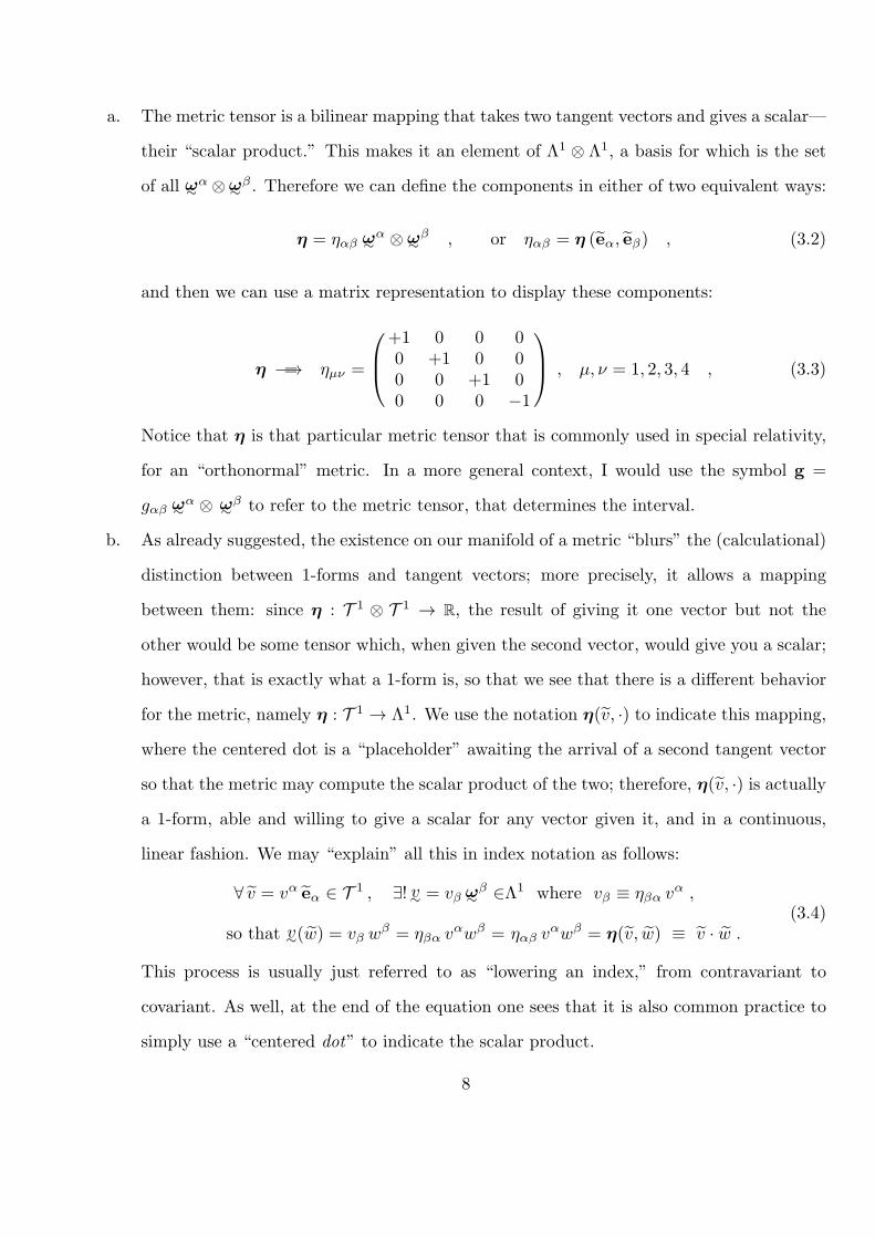
a. The metric tensor is a bilinear mapping that takes two tangent vectors and gives a scalar—

their “scalar product.” This makes it an element of Λ1 ⊗ Λ1, a basis for which is the set

of all ω∼α ⊗ω∼

β . Therefore we can define the components in either of two equivalent ways:

η = ηαβ ω∼α ⊗ ω∼

β , or ηαβ = η (eα, eβ) , (3.2)

and then we can use a matrix representation to display these components:

η =−→ ηµν =

+1 0 0 00 +1 0 00 0 +1 00 0 0 −1

, µ, ν = 1, 2, 3, 4 , (3.3)

Notice that η is that particular metric tensor that is commonly used in special relativity,

for an “orthonormal” metric. In a more general context, I would use the symbol g =

gαβ ω∼α ⊗ ω∼

β to refer to the metric tensor, that determines the interval.

b. As already suggested, the existence on our manifold of a metric “blurs” the (calculational)

distinction between 1-forms and tangent vectors; more precisely, it allows a mapping

between them: since η : T 1 ⊗ T 1 → R, the result of giving it one vector but not the

other would be some tensor which, when given the second vector, would give you a scalar;

however, that is exactly what a 1-form is, so that we see that there is a different behavior

for the metric, namely η : T 1 → Λ1. We use the notation η(v, ·) to indicate this mapping,

where the centered dot is a “placeholder” awaiting the arrival of a second tangent vector

so that the metric may compute the scalar product of the two; therefore, η(v, ·) is actually

a 1-form, able and willing to give a scalar for any vector given it, and in a continuous,

linear fashion. We may “explain” all this in index notation as follows:

∀ v = vα eα ∈ T 1 , ∃! v∼ = vβ ω∼β ∈Λ1 where vβ ≡ ηβα vα ,

so that v∼(w) = vβ wβ = ηβα vαwβ = ηαβ v

αwβ = η(v, w) ≡ v · w .(3.4)

This process is usually just referred to as “lowering an index,” from contravariant to

covariant. As well, at the end of the equation one sees that it is also common practice to

simply use a “centered dot” to indicate the scalar product.

8

c. Clearly the process should have a reverse as well, since we may “undo” the process of

lowering the index by using the inverse matrix for the matrix presenting η, which we can

refer to by the symbol η−1, although we will usually use exactly the same symbol for the

inverse, but with the indices raised:

η−1 =−→ ηµν where ηµνηνλ ≡ δµλ =←− I4 . (3.5)

Having this inverse, we immediately have two different functions that it can perform:

i.) The first is simply that it maps 1-forms to tangent vectors:

η−1 : Λ1 → T 1 ,where ∀α∼ = αµ ω∼µ ∈ Λ1 , ∃! α = αµ eµ ∈ T 1

with αµ ≡ ηµναν and ∀β∼ ∈ Λ1 , β∼(α) = βµ α

µ = βµηµναν .

(3.6)

This process, of course, is referred to as “raising an index,” from covariant to con-

travariant.

ii.) The second function is already put into evidence in the last phrases of the equation

above, namely we may use η−1 as a scalar product in the vector space of differential

forms, Λ1:

η−1 : Λ1 × Λ1 → R , via η−1(α∼, β∼) ≡ ηµν αµβν ≡ α∼ · β∼ ∈ R . (3.7)

Do note that all of the above concerning raising and lowering indices applies

equally well when using some (vector) basis where the metric might have quite a different

form than does the simple, Minkowski presentation of ηµν . Under those circumstances,

we might well refer to the metric as g, although in spacetime this would still be a matrix

with the same signature and significance relative to the interval.

d. The electromagnetic tensor is a skew-symmetric, second-rank tensor, and therefore is

actually a 2-form, i.e., an element of Λ2. Therefore we use the (skew-symmetric) wedge

products that provide a basis for Λ2:

F∼ ≡12Fαβ ω∼

α ∧ ω∼β , (3.8)

9

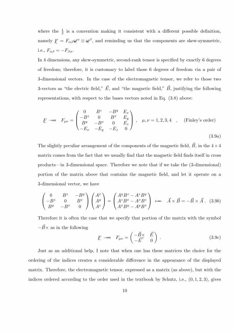
where the 12 is a convention making it consistent with a different possible definition,

namely F∼ = Fαβω∼α ⊗ ω∼

β , and reminding us that the components are skew-symmetric,

i.e., Fαβ = −Fβα.

In 4 dimensions, any skew-symmetric, second-rank tensor is specified by exactly 6 degrees

of freedom; therefore, it is customary to label those 6 degrees of freedom via a pair of

3-dimensional vectors. In the case of the electromagnetic tensor, we refer to those two

3-vectors as “the electric field,” E, and “the magnetic field,” B, justifying the following

representations, with respect to the bases vectors noted in Eq. (3.8) above:

F∼ =−→ Fµν =

0 Bz −By Ex

−Bz 0 Bx Ey

By −Bx 0 Ez

−Ex −Ey −Ez 0

, µ, ν = 1, 2, 3, 4 , (Finley’s order)

(3.9a)

The slightly peculiar arrangement of the components of the magnetic field, B, in the 4×4

matrix comes from the fact that we usually find that the magnetic field finds itself in cross

products—in 3-dimensional space. Therefore we note that if we take the (3-dimensional)

portion of the matrix above that contains the magnetic field, and let it operate on a

3-dimensional vector, we have 0 Bz −By

−Bz 0 Bx

By −Bx 0

Ax

Ay

Az

=

AyBz −AzBy

AzBx −AxBz

AxBy −AyBx

=←− A× B = −B × A . (3.9b)

Therefore it is often the case that we specify that portion of the matrix with the symbol

−B× as in the following

F∼ =−→ Fµν =

(−B× E−ET

0

). (3.9c)

Just as an additional help, I note that when one has these matrices the choice for the

ordering of the indices creates a considerable difference in the appearance of the displayed

matrix. Therefore, the electromagnetic tensor, expressed as a matrix (as above), but with the

indices ordered according to the order used in the textbook by Schutz, i.e., (0, 1, 2, 3), gives

10

the following appearance:

Fαβ =

0 −Ex −Ey −Ez

Ex 0 Bz −By

Ey −Bz 0 Bx

Ez By −Bx 0

, α, β = 0, 1, 2, 3 , (Schutz’s order) (3.9′)

Following our discussion of raising and lowering indices, we may now consider various

different “index locations” for the components of the electromagnetic tensor, all presented,

as usual, in Finley’s index ordering:

Fµν ≡ ηµλ Fλν =−→

+1 0 0 00 +1 0 00 0 +1 00 0 0 −1

0 Bz −By Ex

−Bz 0 Bx Ey

By −Bx 0 Ez

−Ex −Ey −Ez 0

=

0 Bz −By Ex

−Bz 0 Bx Ey

By −Bx 0 Ez

Ex Ey Ez 0

, (3.10)

Fµν ≡ Fµλ η

λν =−→

0 Bz −By Ex

−Bz 0 Bx Ey

By −Bx 0 Ez

−Ex −Ey −Ez 0

+1 0 0 00 +1 0 00 0 +1 00 0 0 −1

=

0 Bz −By −Ex

−Bz 0 Bx −Ey

By −Bx 0 −Ez

−Ex −Ey −Ez 0

. (3.11)

It should be noted that these matrix presentations of the electromagnetic field tensor when

it has one index contravariant and one covariant do not give skew-symmetric matrices.

Skew symmetry on the indices, or symmetry, requires that the indices be of the same type!

11

IV. Display of Matrix Arithmetic without explicit indices

1. Basic Notions:

We sometimes want to conserve ink, and simplify the life of the reader, by not explicitly writing

out the indices on symbols representing matrices. In fact, this justifies the fact that there are

very standard conventions concerning matrix multiplication. To proceed, we first give notation

to relate the statement that some matrix is named A, and the statement that the elements of

that matrix are labelled by the symbols Aαµ through the following convention:

A = ((Aαν)) means A is the matrix with components Aα

ν . (4.1)

Note that the transpose of a matrix requires switching its rows and columns; therefore, we

could have the following examples, where we use an upper T to denote the transpose of a given

matrix:

A = ((Aαν)) ⇐⇒ AT = ((Aν

α)) and B = ((Bab)) ⇐⇒ BT = ((Bba)) . (4.2)

We may then state succinctly the rules concerning matrix multiplication, of two matrices, A

and B, say:

C ≡ AB , ⇐⇒ Cab = Aa

eBeb , (4.3)

where the symbol ⇐⇒ is to be read as meaning “if and only if.”

It is perhaps also worth noting that a matrix with a contravariant row index and a covariant

column index—the most usual form we see—is one that is presenting an operator that maps

tangent vectors into tangent vectors; i.e., we have the following relationship between a linear

operator and its matrix presentation:

A : T 1 → T 1 ⇐⇒ A = ((Aµν)) or, equivalently A =−→ Aµ

ν . (4.4)

This is consistent with our various conventions: we begin with a tangent vector, which has

contravariant indices, and the final result of the action of our operator on that tangent vector

12

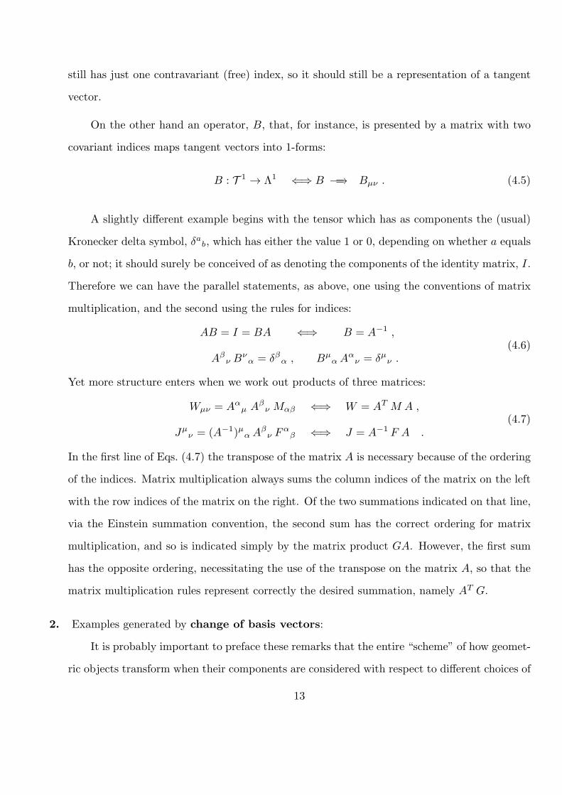
still has just one contravariant (free) index, so it should still be a representation of a tangent

vector.

On the other hand an operator, B, that, for instance, is presented by a matrix with two

covariant indices maps tangent vectors into 1-forms:

B : T 1 → Λ1 ⇐⇒ B =−→ Bµν . (4.5)

A slightly different example begins with the tensor which has as components the (usual)

Kronecker delta symbol, δab, which has either the value 1 or 0, depending on whether a equals

b, or not; it should surely be conceived of as denoting the components of the identity matrix, I.

Therefore we can have the parallel statements, as above, one using the conventions of matrix

multiplication, and the second using the rules for indices:

AB = I = BA ⇐⇒ B = A−1 ,

Aβν B

να = δβα , Bµ

α Aαν = δµν .

(4.6)

Yet more structure enters when we work out products of three matrices:

Wµν = Aαµ Aβ

ν Mαβ ⇐⇒ W = AT M A ,

Jµν = (A−1)µα Aβ

ν Fαβ ⇐⇒ J = A−1 F A .

(4.7)

In the first line of Eqs. (4.7) the transpose of the matrix A is necessary because of the ordering

of the indices. Matrix multiplication always sums the column indices of the matrix on the left

with the row indices of the matrix on the right. Of the two summations indicated on that line,

via the Einstein summation convention, the second sum has the correct ordering for matrix

multiplication, and so is indicated simply by the matrix product GA. However, the first sum

has the opposite ordering, necessitating the use of the transpose on the matrix A, so that the

matrix multiplication rules represent correctly the desired summation, namely AT G.

2. Examples generated by change of basis vectors:

It is probably important to preface these remarks that the entire “scheme” of how geomet-

ric objects transform when their components are considered with respect to different choices of

13

a basis set is the place where more classical (a la 1930’s to, perhaps, 1960’s) treatments, and

definitions, of tensor analysis begin. Therefore, this material is really more important than its

location here might immediately suggest!

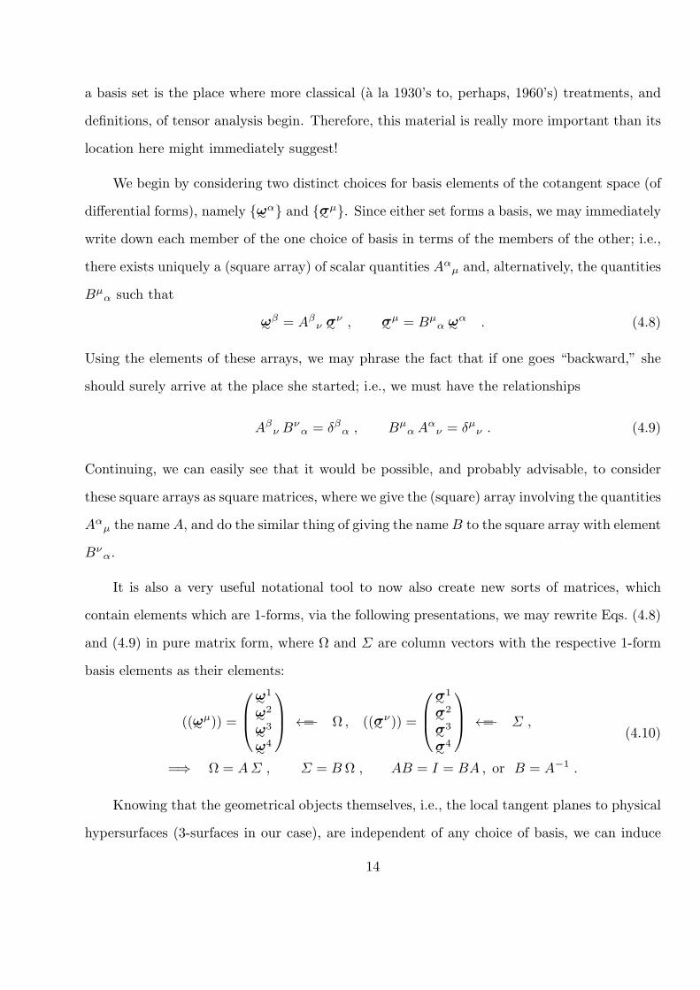
We begin by considering two distinct choices for basis elements of the cotangent space (of

differential forms), namely ω∼α and σ∼µ. Since either set forms a basis, we may immediately

write down each member of the one choice of basis in terms of the members of the other; i.e.,

there exists uniquely a (square array) of scalar quantities Aαµ and, alternatively, the quantities

Bµα such that

ω∼β = Aβ

ν σ∼ν , σ∼

µ = Bµα ω∼

α . (4.8)

Using the elements of these arrays, we may phrase the fact that if one goes “backward,” she

should surely arrive at the place she started; i.e., we must have the relationships

Aβν B

να = δβα , Bµ

α Aαν = δµν . (4.9)

Continuing, we can easily see that it would be possible, and probably advisable, to consider

these square arrays as square matrices, where we give the (square) array involving the quantities

Aαµ the name A, and do the similar thing of giving the name B to the square array with element

Bνα.

It is also a very useful notational tool to now also create new sorts of matrices, which

contain elements which are 1-forms, via the following presentations, we may rewrite Eqs. (4.8)

and (4.9) in pure matrix form, where Ω and Σ are column vectors with the respective 1-form

basis elements as their elements:

((ω∼µ)) =

ω∼

1

ω∼2

ω∼3

ω∼4

=←− Ω , ((σ∼ν)) =

σ∼

1

σ∼2

σ∼3

σ∼4

=←− Σ ,

=⇒ Ω = AΣ , Σ = B Ω , AB = I = BA , or B = A−1 .

(4.10)

Knowing that the geometrical objects themselves, i.e., the local tangent planes to physical

hypersurfaces (3-surfaces in our case), are independent of any choice of basis, we can induce

14

transformations of various other associated objects. We begin with the components of an

arbitrary 1-form τ∼:

τ∼ = τα ω∼α or τ∼ =−→ T ≡ ((τα)) , relative to the basis ω∼α

τ∼ = τ ′µ σ∼µ or τ∼ =−→ T ′ ≡ ((τ ′µ)) , relative to the basis σ∼µ

σ∼µ = (A−1)µα ω∼

α =⇒ τ ′µ = Aαµ τα or T ′ = TA ,

(4.11)

where we have agreed that the matrix presentation of the components of a 1-form, such as τ∼,

being covariant, would be taken as a row-vector, which insures that the order indicated above

for the matrix multiplication is indeed the correct order.

We may then consider the reciprocal bases for tangent vectors, relative to the two bases

ω∼α and σ∼µ, respectively, as follows:

ω∼α(eβ) = δαβ and σ∼

µ(fν) = δµν ,

σ∼µ = (A−1)µα ω∼

α =⇒ fµ = Aαµ eα , or F = EA ,

(4.12)

where we have named the row vectors (with vector entries) called F = ((fµ)) and E = ((eµ)).

This gives us the capability to look at the components of an arbitrary tangent vector, v:

v = vα eα or v =−→ V ≡ ((vα)) , relative to the basis eα

v = v′µ fµ or v =−→ V ′ ≡ ((v′µ)) , relative to the basis fµ

σ∼µ = (A−1)µα ω∼

α =⇒ v′µ = (A−1)µα vα or V ′ = A−1 V ,

(4.13)

where we have agreed that the matrix representation of the components of a tangent vector,

such as v, would be taken as a column-vector, so that the order indicated above for the matrix

multiplication is again the correct order.

Notice that the components of a 1-form, conventionally taken as lower indices, are such

that they transform according to the same matrix, A = B−1, as do the tangent vector basis

elements, eα; it is for this reason that they are referred to as “covariant,” in the sense that

they transform in the same manner. On the other hand, we see that the components of a

tangent vector transform in the inverse manner to the basis elements for tangent vectors, for

which reason they are referred to as “contravariant.”

15

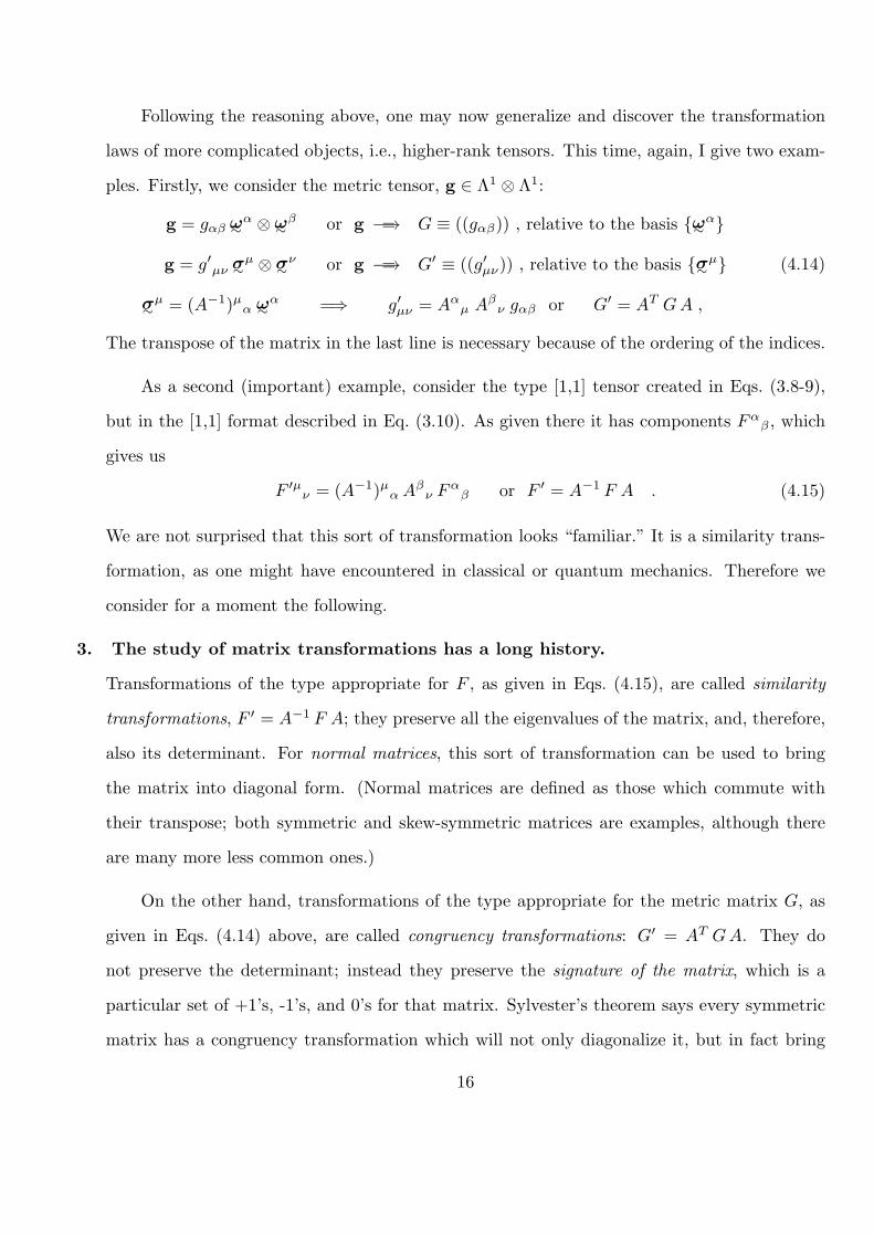
Following the reasoning above, one may now generalize and discover the transformation

laws of more complicated objects, i.e., higher-rank tensors. This time, again, I give two exam-

ples. Firstly, we consider the metric tensor, g ∈ Λ1 ⊗ Λ1:

g = gαβ ω∼α ⊗ ω∼

β or g =−→ G ≡ ((gαβ)) , relative to the basis ω∼α

g = g′µν σ∼µ ⊗ σ∼

ν or g =−→ G′ ≡ ((g′µν)) , relative to the basis σ∼µ

σ∼µ = (A−1)µα ω∼

α =⇒ g′µν = Aαµ Aβ

ν gαβ or G′ = AT GA ,

(4.14)

The transpose of the matrix in the last line is necessary because of the ordering of the indices.

As a second (important) example, consider the type [1,1] tensor created in Eqs. (3.8-9),

but in the [1,1] format described in Eq. (3.10). As given there it has components Fαβ , which

gives us

F ′µν = (A−1)µα Aβ

ν Fαβ or F ′ = A−1 F A . (4.15)

We are not surprised that this sort of transformation looks “familiar.” It is a similarity trans-

formation, as one might have encountered in classical or quantum mechanics. Therefore we

consider for a moment the following.

3. The study of matrix transformations has a long history.

Transformations of the type appropriate for F , as given in Eqs. (4.15), are called similarity

transformations, F ′ = A−1 F A; they preserve all the eigenvalues of the matrix, and, therefore,

also its determinant. For normal matrices, this sort of transformation can be used to bring

the matrix into diagonal form. (Normal matrices are defined as those which commute with

their transpose; both symmetric and skew-symmetric matrices are examples, although there

are many more less common ones.)

On the other hand, transformations of the type appropriate for the metric matrix G, as

given in Eqs. (4.14) above, are called congruency transformations: G′ = AT GA. They do

not preserve the determinant; instead they preserve the signature of the matrix, which is a

particular set of +1’s, -1’s, and 0’s for that matrix. Sylvester’s theorem says every symmetric

matrix has a congruency transformation which will not only diagonalize it, but in fact bring

16

it to have only +1, -1, or 0 in all the places on the diagonal. This set, independent of order,

is called the signature. (Sometimes, only the sum of these quantities is referred to, also, as

the signature; this is completely understandable only when the dimension of the manifold is a

priori known.)

Therefore, in a spacetime, the equivalence principle of Einstein

assures us that there is always a change of basis for T , effected by

an invertible matrix, M , such that the components of the metric

can be converted from gαβ to just those of an arbitrary inertial

frame of special relativity, ηµν :

G = MT HM , or gαβ = Mµα ηµν M

νβ , (4.16)

where the symbol H is a capital Greek η.

This fact assures us that we may always, in some neighborhood of

a given point in spacetime, find a special basis set for which the

components are what they would have been were the spacetime

flat and special relativity valid. It is only to be noted that this

basis set may not be defined everywhere when the spacetime is

not flat.

4. Comments on Determinants of Matrices.

In addition to rules for matrix multiplication, matrices also come equipped with a definition

of various scalars created from them. The only important ones we are likely to use are the

trace, tr A, and the determinant, detA.

a. The definition of trace must be given so that it will be invariant under tensor transforma-

tion rules, i.e., it should be a scalar; therefore, we can write

tr A ≡ Aαα = gαβAβα , (4.17)

17

where gαβ are the components of the inverse metric tensor, if the manifold admits one to

exist there.

If there is no metric tensor, or if it has no inverse, then the trace will not be an invariant

quantity. In addition we should explicitly note that∑4

α=1 Aαα is not the trace, since it

would have a different value in every distinct coordinate basis.

b. The definition of the determinant of an n × n matrix is independent of the properties of

the underlying manifold. It involves taking products of n elements, one from each row

and from each column, in certain orders, with certain signs.

The Levi-Civita symbol, ϵb1b2...bn ≡ ϵb1b2...bn , has n indices, is skew-

symmetric under the interchange of any two of those indices, and is such that

ϵ1234 = +1. Since this statement of numerical value is required to

be true in whatsoever coordinate system, the Levi-Civita symbol

is not a tensor quantity!

It has been defined precisely so that it creates determinants via summations, as expressed

by the Fundamental Theorem of Determinants as written below. In fact this theorem

is simply a mathematical re-phrasing of the language one learned long ago about how to take

determinants, involving “signed minors,” etc.:

ϵb1b2...bn Aa1b1A

a2b2 . . . A

anbn = ϵa1a2...an det(A) . (4.18)

The following rather complicated (numerical) relations involving the values of a product

of Levi-Civita symbols, are worth writing down, since they are occasionally of use, especially

in those cases where one or more pair of the indices are being summed. Their proof is very

straightforward but quite lengthy, and will be omitted here:

ϵa1...an ϵb1...bn =

∣∣∣∣∣∣∣δa1

b1. . . δa1

bn...

. . ....

δan

b1. . . δan

bn

∣∣∣∣∣∣∣ ≡ δa1...an

b1...bn, (4.19)

18

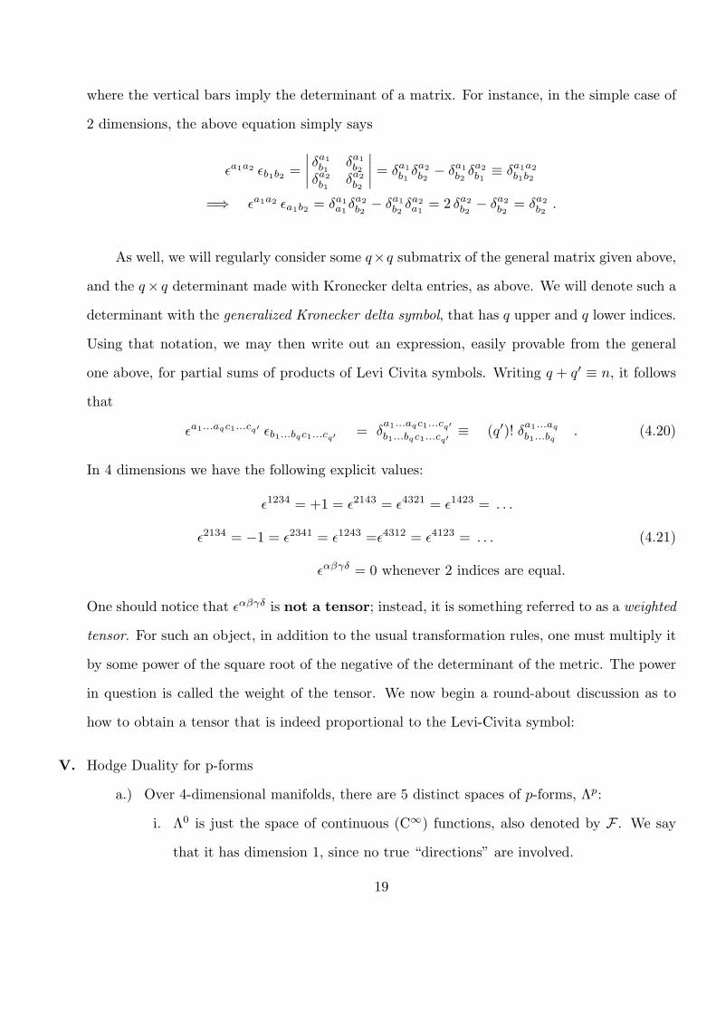
where the vertical bars imply the determinant of a matrix. For instance, in the simple case of

2 dimensions, the above equation simply says

ϵa1a2 ϵb1b2 =

∣∣∣∣ δa1

b1δa1

b2δa2

b1δa2

b2

∣∣∣∣ = δa1

b1δa2

b2− δa1

b2δa2

b1≡ δa1a2

b1b2

=⇒ ϵa1a2 ϵa1b2 = δa1a1δa2

b2− δa1

b2δa2a1

= 2 δa2

b2− δa2

b2= δa2

b2.

As well, we will regularly consider some q×q submatrix of the general matrix given above,

and the q× q determinant made with Kronecker delta entries, as above. We will denote such a

determinant with the generalized Kronecker delta symbol, that has q upper and q lower indices.

Using that notation, we may then write out an expression, easily provable from the general

one above, for partial sums of products of Levi Civita symbols. Writing q + q′ ≡ n, it follows

that

ϵa1...aqc1...cq′ ϵb1...bqc1...cq′ = δa1...aqc1...cq′

b1...bqc1...cq′≡ (q′)! δ

a1...aq

b1...bq. (4.20)

In 4 dimensions we have the following explicit values:

ϵ1234 = +1 = ϵ2143 = ϵ4321 = ϵ1423 = . . .

ϵ2134 = −1 = ϵ2341 = ϵ1243 =ϵ4312 = ϵ4123 = . . .

ϵαβγδ = 0 whenever 2 indices are equal.

(4.21)

One should notice that ϵαβγδ is not a tensor; instead, it is something referred to as a weighted

tensor. For such an object, in addition to the usual transformation rules, one must multiply it

by some power of the square root of the negative of the determinant of the metric. The power

in question is called the weight of the tensor. We now begin a round-about discussion as to

how to obtain a tensor that is indeed proportional to the Levi-Civita symbol:

V. Hodge Duality for p-forms

a.) Over 4-dimensional manifolds, there are 5 distinct spaces of p-forms, Λp:

i. Λ0 is just the space of continuous (C∞) functions, also denoted by F . We say

that it has dimension 1, since no true “directions” are involved.

19

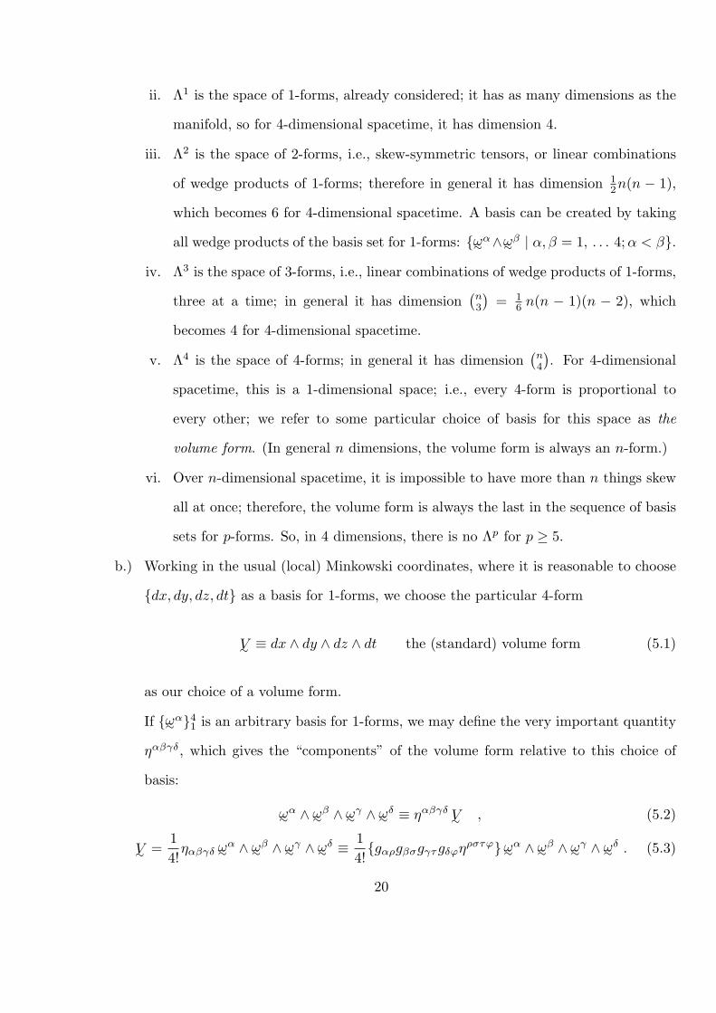
ii. Λ1 is the space of 1-forms, already considered; it has as many dimensions as the

manifold, so for 4-dimensional spacetime, it has dimension 4.

iii. Λ2 is the space of 2-forms, i.e., skew-symmetric tensors, or linear combinations

of wedge products of 1-forms; therefore in general it has dimension 12n(n − 1),

which becomes 6 for 4-dimensional spacetime. A basis can be created by taking

all wedge products of the basis set for 1-forms: ω∼α∧ω∼β | α, β = 1, . . . 4;α < β.

iv. Λ3 is the space of 3-forms, i.e., linear combinations of wedge products of 1-forms,

three at a time; in general it has dimension(n3

)= 1

6 n(n − 1)(n − 2), which

becomes 4 for 4-dimensional spacetime.

v. Λ4 is the space of 4-forms; in general it has dimension(n4

). For 4-dimensional

spacetime, this is a 1-dimensional space; i.e., every 4-form is proportional to

every other; we refer to some particular choice of basis for this space as the

volume form. (In general n dimensions, the volume form is always an n-form.)

vi. Over n-dimensional spacetime, it is impossible to have more than n things skew

all at once; therefore, the volume form is always the last in the sequence of basis

sets for p-forms. So, in 4 dimensions, there is no Λp for p ≥ 5.

b.) Working in the usual (local) Minkowski coordinates, where it is reasonable to choose

dx, dy, dz, dt as a basis for 1-forms, we choose the particular 4-form

V∼ ≡ dx ∧ dy ∧ dz ∧ dt the (standard) volume form (5.1)

as our choice of a volume form.

If ω∼α41 is an arbitrary basis for 1-forms, we may define the very important quantity

ηαβγδ, which gives the “components” of the volume form relative to this choice of

basis:

ω∼α ∧ ω∼

β ∧ ω∼γ ∧ ω∼

δ ≡ ηαβγδ V∼ , (5.2)

V∼ =1

4!ηαβγδ ω∼

α ∧ ω∼β ∧ ω∼

γ ∧ ω∼δ ≡ 1

4!gαρgβσgγτgδφηρστφω∼α ∧ ω∼

β ∧ ω∼γ ∧ ω∼

δ . (5.3)

20

This tensor is completely skew-symmetric, i.e., it changes sign when any two indices

are interchanged, and so must be proportional to the Levi-Civita symbol, ϵαβγδ, used

for determinants. One verifies that the following defines tensors of type [4,0] and [0,4],

respectively, related as usual by raising/lowering of indices via the metric tensor:

ηαβγδ =1

mϵαβγδ , ηαβγδ = (−1)s mϵαβγδ ,

where m ≡ det(M) , G = MT HM ,

g ≡ detG = m2 det(H) =(−1)s m2 , s = 0 or 1 .

(5.4)

Of course the values of ηαβγδ depend on the basis chosen; however, for an orthonormal

tetrad, where the metric components are just ηµν , we have that η1234 = +1 = −η1234.

On the other hand, in ordinary, Cartesian 3-dimensional space, in an orthonormal

frame, we simply have η123 = +1 = η123, as expected.

The following rather complicated relations are worth writing down, since they are

occasionally of considerable use:

ηa1...an ηb1...bn = (−1)s

∣∣∣∣∣∣∣δa1

b1. . . δa1

bn...

. . ....

δan

b1. . . δan

bn

∣∣∣∣∣∣∣ ≡ (−1)s δa1...an

b1...bn, (5.5)

where the vertical bars imply a determinant, and we regularly intend to denote a

q × q determinant made with Kronecker delta entries, as above, with the generalized

Kronecker delta symbol indicated above, that has q upper and q lower indices.

Writing p+ p′ ≡ n, it then follows that

ηa1...apc1...cp′ ηb1...bpc1...cp′ = (−1)s δa1...apc1...cp′

b1...bpc1...cp′= (p′)!(−1)s δa1...ap

b1...bp. (5.6)

c.) the (Hodge) dual, ∗ : Λp −→ Λn−p

Let α∼ be an arbitrary p-form; then we denote the (Hodge) dual by ∗α∼, an (n−p)-form.

They are related as follows:

21

α∼ =1

p!αµ1...µp

ω∼µ1 ∧ . . . ∧ ω∼

µp ,

∗α∼ ≡ipp

′+s

p!(p′)!αb1...bp ηb1...bpc1...cp′ ω∼

c1 ∧ . . . ∧ ω∼cp′ ≡ 1

(p′)!(∗α)c1...cp′ ω∼

c1 ∧ . . . ∧ ω∼cp′ .

(5.7)

The factors of i ≡√−1 have been inserted in just such a way that the dual of the

dual brings one back to where she started:

∗∗α∼ = α∼ . (5.8)

There are various conventions concerning the i’s in the definition. My convention,

using the factors of i, allows for eigen-2-forms of the ∗ operator, since Eq. (5.8)

obviously tells us that the eigenvalues of ∗ are ±1.

d.) Since the definition of (Hodge) duality appears quite complicated, it is worthwhile

writing it down for all plausible exemplars that may occur, in our 4-dimensional

spacetime. We do this for the standard Minkowski tetrad, dx, dy, dz, dt, and the

bases of each Λp:

Λ1 ↔ Λ3 : ∗

dxdydzdt

= −

dy ∧ dz ∧ dtdz ∧ dx ∧ dtdx ∧ dy ∧ dtdx ∧ dy ∧ dz

, Λ0 ↔ Λ4 : ∗1 = −idx ∧ dy ∧ dz ∧ dt ,

Λ2 ↔ Λ2 : ∗

dx ∧ dydy ∧ dzdz ∧ dx

= −i

dz ∧ dtdx ∧ dtdy ∧ dt

, .

(5.9)

As an example, consider the electromagnetic 2-form, in Eqs. (2.8), from which we have:

F∼ =−→ Fµν =

0 Bz −By Ex

−Bz 0 Bx Ey

By −Bx 0 Ez

−Ex −Ey −Ez 0

,

∗F∼ =−→ (∗F )µν =− i

0 −Ez Ey Bx

Ez 0 −Ex By

−Ey Ex 0 Bz

−Bx 0−By −Bz 0

.

(5.10)

22

Note that the map from F∼ to i∗F∼ is accomplished by sending B → −E and E → +B.

e. To complete the picture, we also give details for 3-dimensional, Euclidean space, with

Cartesian basis, dx, dy, dz:

Λ1 ↔ Λ2 : ∗

dxdydz

= −

dy ∧ dzdz ∧ dxdx ∧ dy

, Λ0 ↔ Λ3 : ∗1 = dx ∧ dy ∧ dz .

Valid only in 3-dimensional space, without time as a coordinate.

23