Physiological Data Modeling

ICML 2004

Banff, AL

July 8, 2004

Jack Mott and Matt Pipke

SmartSignal Corporation

SmartSignal Corporation

Incubator of Similarity-Based Modeling technology–Universally applicable–Data driven, empirical–Scalable, deployable

Commercially proven in our eCM software–Delta Airlines – all engines, all flights–Power Plants – Entergy, Dynegy, APS– Transportation – GM-EMD, Caterpillar

Similarity-Based Modeling

Snapshots at instants of time Needs only historical data Removal of normal variations Anomaly detection and isolation One technology for all applications

Similarity-BasedNon-Parametric

Empirical Model

Similarity-BasedNon-Parametric

Empirical Model

Pre

dic

tion

s

Pre

dic

tion

s

Resid

uals

Resid

uals

Ale

rts

Ale

rts

Diagnostics Engine

Diagnostics Engine

Inp

ut

Inp

ut

Physiological Data Modeling Method

A historical H matrix of reference data is first chosen comprising refXi vectors

A local D matrix is chosen comprising a small number of refXi vectors with the highest similarities to a newX vector

Identical vectors have similarity = 1 Non-identical vectors have 0 <= similarity < 1 The newY model vector is given by

newY = D(DT#D) –1(DT #newX) where the similarity operation (#) applies only to

independent variables

Physiological Data

11 independent variables –User characteristics (2)–Armband sensor values (9)

2 dependent variables –Gender number–Annotation class

Training Data Setup

Select 2,500 – 3,000 records for each H matrix–One H matrix for gender–One H matrix for annotation 3004–One H matrix for annotation 5102

Each H matrix– Includes about equal populations for each user– Includes positive and negative examples–Contains no vectors too similar to each other–Contains only filtered data (99% of total)

> User 17 excluded

Gender H Matrix

8

Annotation 5102 H Matrix

8

Annotation 3004 H Matrix

8

Training Data Modeling

If any vector to be modeled was in an H matrix it was removed from the H matrix before the D matrix was formed

Leave-one-out cross-validation of each H matrix– Chose 10 as number of vectors for the D matrices– Reduced the number of independent variables to 8 - 9

Modeled all 580,264 unfiltered training vectors– Inferred gender with gender H matrix– Inferred class with annotation 5102 H matrix

> Positive examples of annotation 5102 have actual class 1> Negative examples of annotation 5102 have actual class 0

– Inferred class with annotation 3004 H matrix> Positive examples of annotation 3004 have actual class 1> Negative examples of annotation 3004 have actual class 0

Gender Windows and Thresholds

Chose gender windows to contain all vectors in a session – If the inferred gender was > T for > ½ the vectors in a

window then all vectors in a window were assigned predicted gender 1, otherwise predicted gender 0

– T = .5 produced Sensitivity = 1 and Specificity = 1

Annotation 5102 Windows and Thresholds

Chose annotation 5102 windows to contain 80 vectors – If the inferred class was > T for > ½ the vectors in a

window then only vectors in a window from the first to last instances where the inferred class was > T were assigned predicted class 1, otherwise predicted class 0

–Sensitivity and Specificity varied as T varied to produce an ROC curve> T = .58 where the slope = 1 on the ROC curve

Window Sizes for Annotation 5102

8

ROC curve for Annotation 5102

8

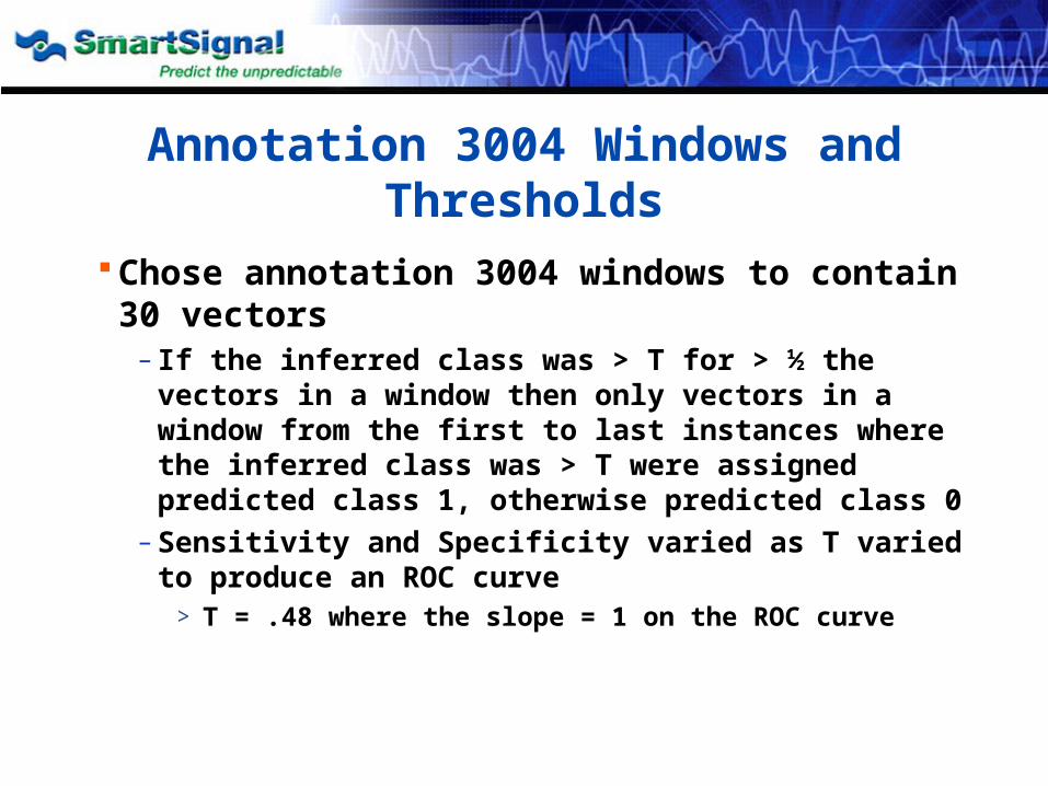
Annotation 3004 Windows and Thresholds

Chose annotation 3004 windows to contain 30 vectors – If the inferred class was > T for > ½ the vectors in a

window then only vectors in a window from the first to last instances where the inferred class was > T were assigned predicted class 1, otherwise predicted class 0

–Sensitivity and Specificity varied as T varied to produce an ROC curve> T = .48 where the slope = 1 on the ROC curve

Window Sizes for Annotation 3004

8

ROC curve for Annotation 3004

8

Training Data Overall Results

Gender Predictions– 23929 (4%) gender 1

> Sensitivity = 23929 / 23929 = 1– 556335 (96%) gender 0

> Specificity = 556335 / 556335 = 1

Annotation 5102 Predictions– 173759 (30%) class 1

> Sensitivity = 96288 / 98172=.98– 406505 (70%) class 0

> Specificity = 72251 / 73668 = .98

Annotation 3004 Predictions– 80511 (14%) class 1

> Sensitivity = 4129 / 4413 = .94– 499753 (86%) class 0

> Specificity = 157993 / 167368 = .94

Test Data Modeling

Modeled all 720,792 unfiltered test vectors–Assumed that characteristic 2 was an extremely important

independent variable in modeling gender–Used the appropriate H matrices, D matrix size,

independent variables, thresholds and window sizes developed from the training data

Predicted gender Predicted class for annotation 5102 Predicted class for annotation 3004

Test Data Overall Results

Gender predictions– 84426 (12%) gender 1

> 4% for training data– 636366 (88%) gender 0

> 97% for training data

Annotation 5102 predictions– 232823 (32%) class 1

> 30% for training data– 487969 (68%) class 0

> 70% for training data

Annotation 3004 predictions– 80511 (11%) class 1

> 14% for training data– 640281 (89%) class 0

> 86% for training data

Conclusions

SBM is easy to apply to real people with real armbands–Modeling choices, the size of D matrix and independent

variables, are determined by only a small fraction of training records, the H matrix

SBM accommodates anomalies in new data– Can be applied to raw, unfiltered data

SBM is automatically user-specific–Presence or absence of a user in new data can be

detected SBM might be made user-general

– Transform data into t-scores with zero mean and unit standard deviation for each activity