physiologically structured population dynamics: a modeling … · 2003-03-12 · physiologically...

Physiologically Structured Population Dynamics:

A Modeling Perspective

B. W. KooiF. D. L. Kelpin

QUERY SHEET

Q1 Au: symbol missing?Q2 Au: OK as meant?Q3 Au: from where?Q4 Au: give location pls.Q5 Au: update available?Q6 Au: add publisher pleaseQ7 Au: Please specify pages

Physiologically Structured Population Dynamics:

A Modeling Perspective

B. W. KooiF. D. L. Kelpin

5Department of Theoretical Biology, Institute of Ecological

Science, Faculty of Earth and Life Sciences,

Vrije Universiteit, Amsterdam,

The Netherlands

In classical population dynamic models all the individuals in a population

10are assumed to be identical or only population averages are considered.

The state of the population is therefore the number of individuals or the

total amount of biomass in the population. The mathematical model is a

first-order ordinary differential equation (ODE) that specifies the time

derivative of this population state. Subsequently, the dynamics of an eco-

15system where populations interact with each other and with their abiotic

environment is usually described by a system of ODEs. The classical

models are sometimes called unstructured population models, as opposed

to structured population models, which take into account the differences

between individuals and characterize an individual by some state. The

20development of this state is modeled from birth till death, often using a

first-order ODE that specifies the time derivative of the individual state.

The model is complemented with models for the birth and death of indivi-

duals. The structured population model is derived straight forwardly from

the individual model using balance laws. The state of a population is no

25longer a single number; it is the distribution of the individuals over

their possible states. If the number of individuals is large, this distribution

is continuous instead of discrete. If, in addition, the distribution is a den-

sity with respect to the individual state, the population model can be writ-

ten as a partial differential equation (PDE). The first structured

3b2 Version Number : 7.00a/W (Sep 25 2000)File path : P:Santype/Journals/Taylor&Francis/Gctb/8(2-3)/8(2-3)-6627/ctb8(2-3)-6627.3dDate and Time : 5/3/03 and 15:20

Address correspondence to B. W. Kooi, Department of Theoretical Biology, Institute of

Ecological Science, Faculty of Earth and Life Sciences, Vrije Universiteit, De Boelelnaan 1087,

1081 HV Amsterdam, The Netherlands. E-mail: [email protected]

We thank Stijntje Kelpin-Vlaskamp for improving the English.

Comments on Theoretical Biology, 8: 1–44, 2003

Copyright # 2003 Taylor & Francis

0894-8550/03 $12.00 + .00

DOI:

1

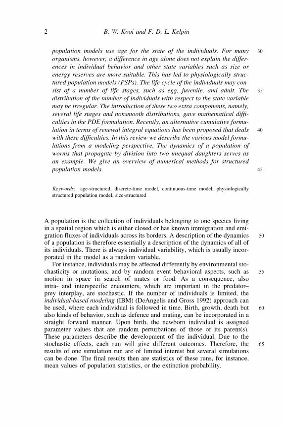
30population models use age for the state of the individuals. For many

organisms, however, a difference in age alone does not explain the differ-

ences in individual behavior and other state variables such as size or

energy reserves are more suitable. This has led to physiologically struc-

tured population models (PSPs). The life cycle of the individuals may con-

35sist of a number of life stages, such as egg, juvenile, and adult. The

distribution of the number of individuals with respect to the state variable

may be irregular. The introduction of these two extra components, namely,

several life stages and nonsmooth distributions, gave mathematical diffi-

culties in the PDE formulation. Recently, an alternative cumulative formu-

40lation in terms of renewal integral equations has been proposed that deals

with these difficulties. In this review we describe the various model formu-

lations from a modeling perspective. The dynamics of a population of

worms that propagate by division into two unequal daughters serves as

an example. We give an overview of numerical methods for structured

45population models.

Keywords: age-structured, discrete-time model, continuous-time model, physiologically

structured population model, size-structured

A population is the collection of individuals belonging to one species livingin a spatial region which is either closed or has known immigration and emi-

50gration fluxes of individuals across its borders. A description of the dynamicsof a population is therefore essentially a description of the dynamics of all ofits individuals. There is always individual variability, which is usually incor-porated in the model as a random variable.

For instance, individuals may be affected differently by environmental sto-55chasticity or mutations, and by random event behavioral aspects, such as

motion in space in search of mates or food. As a consequence, alsointra- and interspecific encounters, which are important in the predator–prey interplay, are stochastic. If the number of individuals is limited, theindividual-based modeling (IBM) (DeAngelis and Gross 1992) approach can

60be used, where each individual is followed in time. Birth, growth, death butalso kinds of behavior, such as defence and mating, can be incorporated in astraight forward manner. Upon birth, the newborn individual is assignedparameter values that are random perturbations of those of its parent(s).These parameters describe the development of the individual. Due to the

65stochastic effects, each run will give different outcomes. Therefore, theresults of one simulation run are of limited interest but several simulationscan be done. The final results then are statistics of these runs, for instance,mean values of population statistics, or the extinction probability.

2 B. W. Kooi and F. D. L. Kelpin

The prospects of applying the IBM approach in ecology is in the possibi-70lity of applying numerical simulations. In general, no mathematical tools are

available to obtain analytical solutions nor to do mathematical analysis.This type of population models can, however, sometimes be analyzed

mathematically with the theory of branching processes (Jagers 1975; Arinoand Kimmel 1989; Jagers 1991; Arino and Kimmel 1993). This theory was

75applied to the analysis of models for cell proliferation by fission. Jagers(1991) describes how the classical Galton–Watson branching process,where the population evolves from generation to generation by individualsgetting an independent and identically distributed (IID) number of children,yields a dichotomy between extinction or unlimited growth.

80This dichotomy results from the fact that the population grows, on aver-age, geometrically with a net reproductive rate equal to the mean numberof offspring. If the expected number of offspring is one or less than one,the population dies out. If it is larger than one, the population growsbeyond all bounds. This means that the population cannot stabilize. If we

85want stabilization to occur, a description of the reproduction of individualsdoes not suffice and the interaction with their environment must be includedin the model.

More elaborate models with different types of individuals can be modeledusing multipoint processes. The dynamics of these populations can be studies

90by individual-based simulations. However, such a simulation is not necessarysince the properties of the population can be analyzed by straightforward gen-eralizations of the analysis for the single-type process (see Caswell and John1992) where a semelparous organism (they die after first reproduction) withfixed generation length is considered.

95The Galton–Watson branching process models only the branching of thefamily trees in the population. No information is specified about the timesat which the branches are formed. However, the age of the individuals andthe ages at child bearing, can be included. Then a mother’s age as well asher type (i-state) determine the starting platform from which the newborn’s

100life is to evolve. This form of dependence between two next generationsleads to a Markov model for the population growth. A superposition of theresulting point processes, essentially Markov renewal theory, provides infor-mation such as the average population growth rate (see Jagers, 1991).

The life cycle of some species can be divided into a number of stages, thus105splitting the population into classes. If the number of individuals in each class

can be written as a linear combination of the class sizes some time step ago,the vector containing all class sizes can be multiplied by a so-called popula-tion matrix to yield the next population state. The elements in this matrix aretransition probabilities from one class into the other, so the matrix is non-

110negative. In the special case where the classes are age classes the matrix iscalled the Leslie matrix and the elements are fecundities on the first rowand survivabilities on the subdiagonal. If the matrix is constant, the modelis linear and the Perron–Frobenius theorem provides conditions for the

Physiologically Structured Population Dynamics 3

convergence to a population state that is the eigenvector belonging to the115dominant eigenvalue.

Once it has reached this state, the population grows geometrically. Eachtime step, the number of individuals in each class is multiplied with the domi-nant eigenvalue. This yields a trichotomy of the following three possibilities.If the dominant eigenvalue is less than one, the population goes extinct. If it is

120larger than one, the population grows without bounds. If it equals one, thepopulation stabilizes.

The entries in the matrix can depend on the population size or explicitly ontime. Then the matrix equations are nonlinear with possibly positive boundedasymptotic behavior. The mathematical analysis of these matrix models is

125worked out in Caswell (1989; 1997), Tuljapurkar (1997), and Cushing(1997).

Stage-structured population models emphasize the stage structure of thepopulations. The development of the population is described by a numberof life-cycle stages, such as eggs, larvae, pupae, and adults. The rate of

130change of the stage size must equal the difference between total recruitmentand loss rates for the stage. Each term in these equations is related to stage-rate processes such as recruitment, death, and maturation, for each stage. Theparameters in these equations are stage-dependent mean value rates, forinstance, death and birth rates. These balance equations form the dynamic

135equations for each stage where the number of individuals in the differentstages are the population state variables, called p-state variables. The resultingpopulation dynamic model is generally described by delay differential equa-tions (DDEs). This type of model is worked out in Nisbet (1997). Thieme(2003) discusses a stage-structured population model where the definition

140of a density-dependent transition rate from one stage into the other enablesa formulation in terms of ODEs, which are easier to handle than DDEs.

In the more general physiologically structured population models, eachindividual is described by its so-called i-state, which contains a number ofphysiological traits such as age, energy, or size. If the number of individuals

145is sufficiently large, a deterministic model can be used (see Metz and de Roos1992). The individual model is described by individual rates, such as birth,growth, and death rates that describe the change of the momentary i-statesof the individual. The deterministic ODE model for the individual togetherwith balance laws directly leads to a PDE model formulation at the popula-

150tion level.In special cases the PDE model can be reduced to an equivalent DDE or an

ODE for a p-state variable such as the total number or biomass of all indivi-duals that make up the population. The later case presents unstructuredmodels that average over the i-state distribution in the population without

155loss of information. It is a special case of a technique referred to as thelinear chain trick. Then the model is reduced to a number of coupledODEs being a closed, finite-dimensional system for moments of the biomassweighted with powers of size (see Metz and Diekmann 1989).


The interplay with the environment is of paramount importance for the160techniques that can be used to analyze the resulting model. If the environment

is assumed to be constant, the model is linear and mathematical techniquesare available to prove existence, uniqueness, and positivity of a solution.As we mentioned earlier, linear models show a trichotomy between extinc-tion, stabilization, and unlimited growth of the population. Stabilization

165only occurs for specific parameter values. If the population has a time-dependentfood source or suffers from a nonconstant predation pressure, the food or thepredator has to be modeled explicitly as well. The resulting nonlinear modelis autonomous. If the environment changes explicitly with time (seasonal ordaily fluctuations) the resulting model is nonautonomous. Generally, in these

170last two cases the model is nonlinear and consequently more difficult to ana-lyze. Often a middle course is adopted in which the vital rates, such as birthrate, growth rate, and death rate, are density dependent; that is, they dependon the population size (number of individuals or total mass), thus implicitlymodeling the effect of the environment on the individual life history.

175These models are often called semilinear. In nonlinear and semilinearmodels, biologically realistic positive bounded solutions can occur for largeparameter ranges.

Age has often been chosen to describe the state of an individual; in addi-tion, the birth and death rate depend solely on age. For continuous-time pro-

180blems without any interplay with the environment the resulting model is alinear first-order PDE for the density function. Webb (1985) analyzes non-linear versions of this PDE model. Properties such as the existenceand uniqueness of the solution are studied and, with respect to long-termdynamic behavior, existence of a so-called equilibrium or stable age

185distribution is important.For many biological systems, age is not appropriate to characterize the

state of an individual. Other i-state variables such as size, energy, or masshave been proposed leading to a class of models called physiologicallystructured population models (PSPs), which are formulated and analyzed

190in Metz and Diekmann (1986) and de Roos (1997). If the environment isconstant it is, however, always possible to use age as the individualstate variable.

Traditionally, the PDE was used. Thieme (1988) works out an examplethat shows that PDE model formulations can be ill-posed. Diekmann et al.

195(1998; 2001) propose a cumulative approach where a description of the lifecycle of each individual is the starting point for the derivation of the popula-tion model formulation. Here ingredients from the theory of multitypebranching processes are used. Mathematically this leads to renewal integralequations (RIEs). In the 2001 paper, the nonlinear case is discussed, where

200interplay with a time-dependent environment is allowed.There is considerable literature on the dynamics of a population consisting

of individuals that propagate by binary fissions. Division can be seen as abirth and death at the same time. The mother dies but two or more daughters


are born at the same time. Division can occur at different i-states. This situa-205tion corresponds to a stochastic life length of the cell. Bell and Anderson

(1967), Sinko and Streifer (1971), Metz and Diekmann (1986) assume thatthe number of individuals is large and that there is a population densityand analyze the deterministic PDE formulation. Diekmann et al. (1993)assume that the population size is large, but allow for measures and analyze

210a cell cycle model using the theory based on renewal equations describing thecumulative effect of divisions.

Models for the cell cycle of the majority types of cells including bacteria,unicellular eukaryotic organisms, and mammalian cells have been developedand described in Lasota and Mackey (1984) and in Tyson and Hannsgen

215(1985; 1986). They propose and analyze a model where cells divide intotwo equal daughter cells. The random division time of the daughters is cor-related to that of the mother. In Metz and Diekmann (1986) and Diekmannet al. (1993), the division time of the daughters is also random, but withthe same distribution for all cells. In both formulations there is no stable

220age-distribution when the cells grow exponentially.Lasota and Mackey (1984) discuss cell cycle models in terms of Markov

operators. These operators connect the density function of the age or massdistribution at birth over generations. The age-dependent cell generationtime case is worked out in Tyrcha (2001). It is assumed that the mass

225dynamics obeys a first-order autonomic ODE. The generation time is thesum of a random variable plus a constant time after the initiation of theDNA synthesis that triggers the cell to transverse through subsequentphases of the cell cycle that have approximately a constant length. Thisapproach gives alternative proof of the fact that there is no stable mass dis-

230tribution of the cells that grow exponentially.Many sciences study the link between what is happening at the single-

particle scale and what can be observed among large populations of particles.We mention population balance models (PBMs) which have been used inchemical engineering since the 1960s (see Fredrickson, 1991; Ramkrishna

2352000; Fredrickson and Mantzaris 2002; and references therein).In this review we restrict our attention to ecology, in particular to one popu-

lation that lives in a spatially homogeneous environment. Only physiologicaltraits, such as age, size, and energy reserves, serve as individual state variables.We discuss various model formulations, starting with age-structured

240models and proceeding to PSP models. The interplay between the choiceof the mathematical model formulation and the features of the biologicalsystem is emphasized.

Generally, no closed-form solutions can be derived for the transient orshort-term dynamics and numerical techniques have to be used to approxi-

245mate the solution. We describe the most popular numerical methods.We elaborate one example in great detail in which the various model

formulations as well as their mathematical and numerical analysis areelucidated. We consider the dynamics of a population of worms which


propagate by division into two unequal daughters. We restrict ourselves to the250case where there is an abundant food supply. In this type of continuous-time

problems it is sometimes advantageous to look for an equivalentdiscrete-time model formulation. For long-term population dynamics theratio of the interdivision times of the two sisters is crucial. Convergence to astable age or size distribution depends on whether this ratio is a rational or

255irrational number.

STRUCTURED POPULATION MODELS

All individuals in a population share the same species-specific behavior.This behavior generally depends not only on environmental conditions butalso on the internal state of the individual. Unstructured population models

260assume that all the individuals are identical. Structured population models,however, allow for differences between individuals. Each individual has itsown internal i-state x. This i-state may vary in time. It necessarily containsall intrinsic information needed to define individual behavior for givenenvironmental conditions. The model for the individual defines the indivi-

265dual’s behavior and the development of its i-state as a function of its envir-onment E and its internal i-state x.

In the previous paragraph, the precise meaning of the word ‘‘behavior’’was deliberately not specified. Whole ranges of models can be thought upto describe one particular population, depending on what is considered to

270be its relevant behavior. These models differ in their level of detail, butalso in the mechanisms that they focus on. There is not one single correctmodel for a population. The choice of model, and as a result of that alsothe contents of the i-state, depend on the model’s intended use.

First, we discuss age-structured models, which have one single i-state vari-275able, the age a of an individual. They are a subgroup of physiologically struc-

tured population models (PSP models), in which the i-state variablesrepresent physiological properties of the individual.

Age-Structured Population Models

Consider the following age-structured population model. Individuals are280born with age 0 and may live up to a maximum age o. The survival function

FðaÞ specifies the probability that an individual survives to age a. So F is anonincreasing function with Fð0Þ ¼ 1 and FðoÞ ¼ 0. The maternity func-tion bðaÞ is defined such that bðaÞ da is the number of newborns motheredby an individual from age a to age aþ da. We look at several classical

285continuous-time and discrete-time formulations of this model, where wepartly follow Kot (2001).


Continuous-Time Renewal Integral Equation

Lotka’s model (Sharpe and Lotka 1911) is a continuous-time model thattracks the population’s birth rate. Let bðtÞ dt be the number of births during

290time interval t to t þ dt. Then Lotka’s model reads

bðtÞ ¼Z t

0

bðt � aÞFðaÞbðaÞ daþ GðtÞ ð1Þ

where GðtÞ, the contribution of all individuals already present at t ¼ 0, isdefined by

GðtÞ ¼Z o�t

0

nð0; aÞ Fðaþ tÞFðaÞ bðaþ tÞ da ð2Þ

295Here nð0; aÞ equals the age density distribution of the initial population; thatis, nð0; aÞ da equals the number of individuals of age a to aþ da at time 0.Notice that GðtÞ ¼ 0 for t > o, in which case the resulting integral equation,Eq. (1), is homogeneous.

Discrete-Time Renewal Equation

300The time t and also age a are now integers. Mathematically the renewalequation yields a difference equation of the form

bt ¼Xt

a¼1

bt�aF aba þ Gt ð3Þ

where

Gt ¼Xo�t

a¼1

n0;a

F aþt

F a

baþt ð4Þ

305The functions bt and Gt have the same meaning as in the continuous-timecase except now at fixed census time intervals. An example of a renewalequation is the Fibonacci (1202) series

bt ¼ bt�1 þ bt�2 ð5Þ

where the number of newborn rabbits bt is the sum of the number of births310one (bt�1) and two time intervals ago (bt�2). In Eq. (3) we have F a ¼ 1

for all a (no mortality) and b1 ¼ 1, b2 ¼ 1, and ba ¼ 0 for a > 2 (one new-born at two preceding time points).


Discrete-Time Leslie Matrix

Here the state is described by the age distribution in discrete points in time315and age. The classical Leslie matrix reads

n0ðtÞn1ðtÞ...

..

.

no�1ðtÞ

0BBBBB@

1CCCCCA

¼

F0 F1 � � � � � � Fo�1

P0 0 � � � 0 0

0 P1. .. . .

. ...

..

. . .. . .

.0 0

0 � � � 0 Po�2 0

0BBBBBB@

1CCCCCCA

n0ðt � 1Þn1ðt � 1Þ

..

.

..

.

no�1ðt � 1Þ

0BBBBB@

1CCCCCA

ð6Þ

We give the Fibonacci series as a example. Then o ¼ 2 and F0 ¼ F1 ¼P0 ¼ 1, leading to

n0ðtÞn1ðtÞ

� �¼ 1 1

1 0

� �n0ðt � 1Þn1ðt � 1Þ

� �ð7Þ

320which is equivalent to the two equations

n0ðtÞ ¼ n0ðt � 1Þ þ n1ðt � 1Þ ð8Þn1ðtÞ ¼ n0ðt � 1Þ ð9Þ

Substitution of n1ðtÞ of the second equation in the first equation gives thefamiliar Eq. (5), now for n0: n0ðtÞ ¼ n0ðt � 1Þ þ n0ðt � 2Þ. Indeed, theterm n0ðtÞ is associated with the birth bt rate of the previous paragraph.

325This is the general procedure to derive from a higher order difference equa-tion a set of first-order difference equations, similar to the procedure in ordinarydifferential equations.

Let NðtÞ denote the total number of individuals at time t. Then we haveNðtÞ ¼ n0ðtÞ þ n1ðtÞ ¼ n0ðt þ 1Þ; that is, the number of individuals at time

330t equals the number of individuals that will be born at t þ 1. Indeed, inthis biological interpretation both classes reproduce at the same time andgive birth to one child. This simple example shows that the number of indi-viduals in the population is just the summation of the number of individualsborn and that survive (all survive in this example) whereby the summation is

335over all possible instants individuals were born (two in this example).

Continuous-Time Partial Differential Equation

Let nðt; aÞ denote the population age-distribution function and hencenðt; aÞ da the number of individuals of age a to aþ da at time t. TheMcKendrick–von Foerster equation (McKendrick, 1926; von Foerster


3401959) reads

@nðt; aÞ@t

þ @nðt; aÞ@a

¼ �dðt; aÞnðt; aÞ ð10Þ

where dðt; aÞ is the per capita mortality rate. The boundary condition at agezero is

nðt; 0Þ ¼Z o

0

nðt; aÞbðt; aÞ da ð11Þ

345where bðt; aÞ is the per capita birth rate. Observe that we should multiply theleft-hand side with da=dt but since it is dimensionless and equals one, it isgenerally omitted. The initial condition completes the mathematical formula-tion and reads

nð0; aÞ ¼ n0ðaÞ ð12Þ

350The resulting model is a first-order linear PDE and mathematical theoryexists dealing with the most important issues such as existence and asymptoticage distribution. To that end the problem is formulated in the framework ofthe theory of semigroups of linear operators (see Webb 1985).

In order to derive a link with Lotka’s model [Eq. (1)]; we assume that the355birth rate and death rate depend only on age, that is, b ¼ bðaÞ and d ¼ dðaÞ.

The survivorship FðaÞ is linked to the death rate by dF=da ¼ �dðaÞ whereFð0Þ ¼ 1. With bðtÞ ¼ nðt; 0Þ we have for t > o, nðt; aÞ ¼ bðt � aÞFðaÞ.Substitution into Eq. (11) yields the Lotka equation, Eq. (1). Similarly, theequivalence can be shown for t � o.

360The case of asynchronous exponential growth, where the number of indi-viduals grows or dies out exponentially but their distribution over the i-statespace stabilizes, is often observed, for instance, in models where all indivi-duals at all time contribute to reproduction and all individuals interactthrough one food resource. This can be seen as follows. Suppose there is

365exponential growth, hence bðtÞ ¼ expfrtg. Substitution into Eq. 1 wheret > o gives the characteristic equation, called the Euler–Lotka equationZ o

0

FðaÞbðaÞ expf�rag da ¼ 1 ð13Þ

It has exactly one real root r ¼ m, the population growth rate.In Figure 1 the solution nðt; aÞ of Eq. (10) is shown where the initial age

370distribution, seen on the left above the line t ¼ 0 (the age axis), is uniform.This unnatural initial condition leads to a discontinuity of the densitywhich propagates along the line t ¼ a. For t > o this discontinuity disappearsand eventually the distribution converges to the stable age distribution, seenon the right. The rates bðaÞ and dðaÞ are such that the population size

375NðtÞ ¼Ro

0nðt; aÞ da blows-up as is clear from Figure 2 where the size NðtÞ

is plotted as function of the time t.


FIGURE 1 Solution of the linear McKendrick–von Foerster equation, Eqs. (10), (11),

(12), with a ¼ 0:5, o ¼ 1, bðaÞ ¼ 0 0 � a < a5 a � a � 1

�, dðaÞ ¼ 1, and n0ðaÞ ¼ 1.

FIGURE 2 Total number of individuals NðtÞ for the solution of the linear

McKendrick–von Foerster equation plotted in Figure 1.


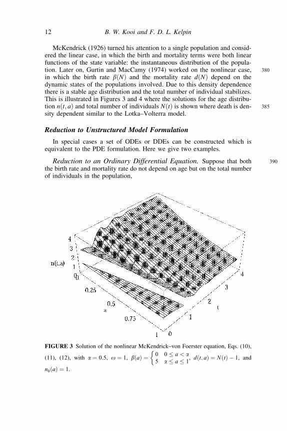
McKendrick (1926) turned his attention to a single population and consid-ered the linear case, in which the birth and mortality terms were both linearfunctions of the state variable: the instantaneous distribution of the popula-

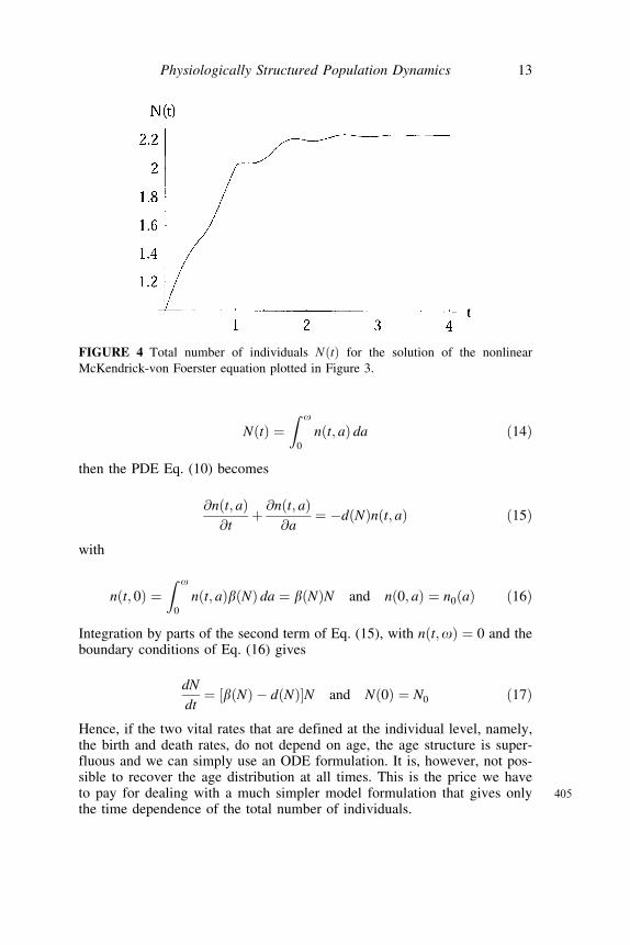
380tion. Later on, Gurtin and MacCamy (1974) worked on the nonlinear case,in which the birth rate bðNÞ and the mortality rate dðNÞ depend on thedynamic states of the populations involved. Due to this density dependencethere is a stable age distribution and the total number of individual stabilizes.This is illustrated in Figures 3 and 4 where the solutions for the age distribu-

385tion nðt; aÞ and total number of individuals NðtÞ is shown where death is den-sity dependent similar to the Lotka–Volterra model.

Reduction to Unstructured Model Formulation

In special cases a set of ODEs or DDEs can be constructed which isequivalent to the PDE formulation. Here we give two examples.

390Reduction to an Ordinary Differential Equation. Suppose that boththe birth rate and mortality rate do not depend on age but on the total numberof individuals in the population,

FIGURE 3 Solution of the nonlinear McKendrick–von Foerster equation, Eqs. (10),

(11), (12), with a ¼ 0:5, o ¼ 1, bðaÞ ¼ 0 0 � a < a5 a � a � 1

�, dðt; aÞ ¼ NðtÞ � 1, and

n0ðaÞ ¼ 1.


NðtÞ ¼Z o

0

nðt; aÞ da ð14Þ

then the PDE Eq. (10) becomes

@nðt; aÞ@t

þ @nðt; aÞ@a

¼ �dðNÞnðt; aÞ ð15Þ

with

nðt; 0Þ ¼Z o

0

nðt; aÞbðNÞ da ¼ bðNÞN and nð0; aÞ ¼ n0ðaÞ ð16Þ

Integration by parts of the second term of Eq. (15), with nðt;oÞ ¼ 0 and theboundary conditions of Eq. (16) gives

dN

dt¼ ½bðNÞ � dðNÞ�N and Nð0Þ ¼ N0 ð17Þ

Hence, if the two vital rates that are defined at the individual level, namely,the birth and death rates, do not depend on age, the age structure is super-fluous and we can simply use an ODE formulation. It is, however, not pos-sible to recover the age distribution at all times. This is the price we have

405to pay for dealing with a much simpler model formulation that gives onlythe time dependence of the total number of individuals.

FIGURE 4 Total number of individuals NðtÞ for the solution of the nonlinear

McKendrick-von Foerster equation plotted in Figure 3.


Reduction to a Delay Differential Equation. Now we assume thatthere are two life stages, juvenile and adult. The individual mature at age a.The birth rate and mortality rate functions are only positive in the age interval

410ða;oÞ. Thus, we assume that the juveniles do not die. We perform a reductionprocedure similar to the one used in the previous section. There are two age-distribution functions, and their dynamics are described each by a PDE:

@nJðt; aÞ@t

þ @nJðt; aÞ@a

¼ 0;@nAðt; aÞ

@tþ @nAðt; aÞ

@a¼ �dðNAÞnAðt; aÞ ð18Þ

with boundary conditions

nJðt; 0Þ ¼ bðNAÞZ o

anðt; aÞ da nJðt; aÞ ¼ nAðt; aÞ nAðt;oÞ ¼ 0 ð19Þ

Let NJ ¼R a

0nJðt; aÞ da denote the number of juveniles and NA ¼Ro

a nAðt; aÞ da the number of adults. Integration of Eq. (18) using the bound-ary conditions of Eq. (19) gives

dNA

dt¼ bðNAÞNAðt � aÞ � dðNAÞNAðtÞ ð20Þ

420with initial function NAðtÞ ¼ NA0 for �a � t � 0. In a similar way we obtaina DDE for the number of juveniles NJðtÞ

dNJ

dt¼ bðNAÞNAðtÞ � bðNAÞNAðt � aÞ ð21Þ

As this involves NAðtÞ, one first has to calculate the number of adults NAðtÞand afterward the number of juveniles NJðtÞ. This last equation shows that the

425change in the number of juveniles equals the difference in population birthrate at t (the newborn) minus the population birth rate at t � a (the individualsthat mature at t and were born a ago).

Physiologically Structured Population Model

In Kooijman (2000) it is argued that age is in many cases not an appropri-430ate state variable to describe the growth and development of a population. As

an example, consumption of food depends on sizes and the waterfleaDaphnia magna typically has a length of 2.5mm at the onset of reproduction.Size differences are also essential in models of cannibalistic populations(Diekmann et al. 1986; van den Bosch et al. 1988; Kirkilionis et al. 2001;

435Claessen et al. 2000; Claessen and Dieckmann 2002) where large adults eatsmall juveniles. For bacteria there is a similar situation. The DNA duplicationis triggered upon exceeding a fixed cell size and DNA duplication lasts


a fixed time period (see Donachie, 1968). Hence the division of an individualdoes not occur at a specific age, but size is also involved.

440Furthermore, many species go through different life stages. In Kooijman(2000) three stages in the life history of individuals are recognized: egg, juve-nile, and adult. Eggs neither eat nor reproduce, juveniles eat but do not repro-duce, and adults both eat and reproduce.

In the PSP model formulation, age is therefore replaced or augmented with445other state variables such as size=mass or energy content. The type of infor-

mation stored in the i-state varies from model to model, but in many cases x isan n-dimensional vector. Each number in this vector then represents a physio-logical trait of the individual.

Recently, models have been proposed where the i-state is a two-450dimensional vector. Droop (1973) introduced the concept of cell nutrient quota

(internal nutrient density) besides biomass in a model for phytoplanktongrowth. In this model, growth is decoupled from nutrient uptake. Phyto-plankton cells store nutrients and the growth rate of a cell depends on theamount of stored nutrient. Hallam et al. (1990) describe a model in which an

455organism consists of storage: lipids, the major source of energy, and astructural component—nonlipid dry material consisting mostly of proteinsand carbohydrates. In Persson et al. (1998) the components are called thereversible and irreversible mass. In reversible mass they include energyreserves such as fat, muscle tissue, and gonads, and in irreversible mass they

460include compounds like bones and organs, which cannot be starved away bythe consumer. The Dynamic Energy Budget (DEB) model (Kooijman 2000),deals with storage materials (reserves) and structural biomass. Here thestorage materials are carbohydrates and lipids but also a part of ribosomalRNA and of the proteins (see Hanegraaf et al. 2000). The storage materials

465have a dual function as a reserve pool for energy and elementary compounds.These storage materials are continuously used and replenished, whilestructural materials are permanent and require maintenance. The reservesadapt to the external food availability, that is, to the environment. If this foodavailability is constant or varies slowly compared to the adaptation process,

470the energy reserves will be in or near their equilibrium state. Individuals willnot be spread out all over the i-state space, but concentrated on or near theline through these equilibrium values for energy reserves.

Given a PSP model, the set of all possible i-states is called the i-state spaceO. If the individual goes through different life stages, O may be divided into

475subsets Oi (e.g., OE; OJ ; OA for the egg, juvenile, and adult stage). Theboundaries of these subsets mark points where the individuals move fromone life stage to the next, such as where they hatch or mature.

As we saw in the age-structured model formulation, the p-state of thepopulation can be a number or mass density that depends on the

480i-state variables. This leads to a PDE formulation for the population withboundary and initial conditions similar to the age-structured case described inthe previous section.


In Diekmann et al. (1998) the mathematical difficulties that may arise inthis formulation are explained in biological terms as follows. In order to keep

485models parameter scarce, one wants to allow for discontinuities with respectto i-state of rates (think of waterflies that start to reproduce upon reaching acritical size; see Thieme 1988). Now consider a situation in which the i-stateof some individual moves in O for an extended period of time along a line ofdiscontinuity of the rate of offspring production, that is, the line that separates

490OJ and OA. Then the model is not acceptable as a model and one should notexpect that existence and uniqueness of solutions at the p-level holds.Whether this phenomenon actually occurs or not in a specific model, ishidden in the rates. It is the combined global effect of the rates that makesthe difference between the model being ill- or well-posed.

495In this section we first introduce the model ingredients. Then we showhow in one big step the behavior of all the individuals in a population islifted to the population level. We start with the classical formulation ofPSP models (Metz and Diekmann 1986), which uses densities and leads toa partial differential equation with boundary and initial conditions. Then

500we continue with the more recently developed cumulative formulation lead-ing to a renewal integral equation.

i-State Formulation

If the individuals go through life stages, the population is split into subpo-pulations that contain the individuals in each life stage. We now describe the

505dynamics for one single population or subpopulation. Later on, boundaryconditions will connect the subpopulations at the borders of their respectivesubspaces Oi. In the PDE formulation, an i-state space O (or Oi) always is asubset of Rn, for some n. The i-states in different life stages may have differ-ent interpretations and their dimension may vary from one stage to another.

510Typical instantaneous vital rates that describe the temporal change of thei-state variable are the growth, birth, and death rates, which will occur asper capita rates at the population level.

Growth Rate. Since we assume that the environment is homogeneous inspace, the spatial coordinates of an individual are irrelevant for its behavior.

515The coordinates of its i-state x, however, follow a trajectory through O.The growth rate gðE; xÞ 2 Rn defines a vector field on O that determines

the speed and direction of this movement through i-state space. Thisimplies that individual growth is deterministic. Note that entries of g donot refer to the physiological ‘‘growth’’ rate if the corresponding i-state

520is not size. If gi represents growth it is sometimes allowed to havegiðE; xÞ < 0 >, that is, a shrinking individual. This can lead to hardmathematical problems and therefore it is generally assumed thatgiðE; xÞ > 0; that is, the direction of the movement is never reversed andthe movement never stops.


525Death Rate. Death removes an individual from the population. Death ismodeled by specifying the death rate dðE; xÞ � 0. The environmental con-dition that influences the death rate generally is predation pressure. Emi-gration or harvest of individuals from the region under consideration can alsobe modeled using the death rate.

530Birth Rate. Different reproduction modes exist. Some of these can bemodeled using an individual birth rate bðE; xb; xÞ � 0. This is the rate atwhich an individual with state x produces offspring with state at birth xb.Often the support of this function is some OA � O, the subset of adults.

Influence on the Environment=Feeding=Predation. The environment535EðtÞ can represent food consumed by the population. When food is abundant

the growth rate does not depend on the food (gðxÞ). On the other hand, whenfood is limiting, growth depends on the food availability (gðEðtÞ; xÞ). In thelatter case the amount of food available depends on the population size sincethis determines how much food is consumed. This feedback interplay is

540typical for predator–prey, or similar trophic, interactions in ecologicalcommunities. In a similar way the population can be consumed by anotherpopulation in which case the death rate stands for natural death rate pluspredation rate (dðEðtÞ; xÞ).

If food is assumed to be an abiotic nutrient which is supplied to the region545where the population lives in, the dynamics of this nutrient is generally

described by an ODE. In case of interplay with other populations they canbe described by one or more ODEs or even PDE.

The growth process is new with respect to age-structured populationmodels. That is, when gðEðtÞ; xÞ ¼ 1, where x is one-dimensional, we get

550essentially an age-structured population model. As mentioned earlier, theenvironment sometimes implicitly modeled as density-dependent birth anddeath rates. Murphy (1983) studies a model with a density-dependentgrowth rate.

p-State Formulation

555The state of the population (the p-state) is now represented by a continu-ous number density function nðxÞ. The integral of this density function overan area of i-states equals the total number of individuals in that area. To be abit more precise, for any measurable set o � O,

Ro nðxÞ dx equals the number

of individuals in the population with i-states in o. To express the fact that this560p-state changes in time, we will denote it as nðt; xÞ, where x is a vector if the

i-state space is multidimensional.

Field Equation. The p-state can be shown (see for instance Metz andDiekmann, 1986, 14), to satisfy the PDE


@nðt; xÞ@t

þXi

@

@xigðEðtÞ; xÞnðt; xÞð Þ ¼ �dðEðtÞ; xÞnðt; xÞ ð22Þ

565or shorter

@nðt; xÞ@t

þ H � gðEðtÞ; xÞnðt; xÞð Þ ¼ �dðEðtÞ; xÞnðt; xÞ ð23Þ

This basically is a transport equation with velocity g, but with a nonzeroright-hand side, which represents the death of individuals.

Boundary Conditions. Individuals may be born on @O, the border of O.570Only part of this border, @þO, is of interest. This is because the growth vector

gðE; xÞ should point inward. Otherwise newborn individuals will leave O,which they are not supposed to do. In mathematical terms: Birth only occursin i-states xb 2 @þO, where the inner product of g with the inward-pointingnormal n is positive. Then the boundary condition reads

nðxbÞ � g EðtÞ; xbð Þnðt; xbÞ ¼ZObðEðtÞ; xb; xÞ nðt; xÞ dx xb 2 @þO ð24Þ

This is sometimes also called the renewal equation.

Initial Conditions. Initial conditions complete the mathematical for-mulation:

nð0; xÞ ¼ n0ðxÞ x 2 O0 ð25Þ580where O0 � O is the support of the density n.

In Murphy (1983) the PDE and its boundary and initial conditions aretransformed from numbers density into biomass density. The resulting PDEformulation is the same as Eqs. (23), (24), and (25), but the interpretationsof some coefficients differ. We remark that in general this transformation

585is not needed.If the dynamics of the environment, for instance, nutrients or predators,

are described by an ODE, the initial amount of these substances completesthe initial conditions and that ODE is solved together with the PDE for thepopulation. Just as in density-dependent age-structured models, also in PSP

590models the birth, growth, and death rates can be assumed to be density depen-dent in order to avoid modeling the food or predator explicitly.

For populations that propagate by binary fission birth rate and death rate(division rate) are coupled. If division is into two equal daughters the result-ing PDE reads:

@nðt; a; vÞ@t

þ @nðt; a; vÞ@a

þ @gðt; a; vÞnðt; a; vÞ@v

¼ � bðt; a; vÞ þ dðt; a; vÞ½ �nðt; a; vÞ þ 2 2bðt; a; 2vÞnðt; a; 2vÞ½ � ð26Þ


where bðt; a; vÞ is now the per capita division rate and dðt; a; vÞ the death rate,that is, here the disappearance of individuals by causes other than division.The terms of the left-hand side are the same as before, but those of theright-hand side are sink and source terms associated with division. If an indi-

600vidual with size v divides, the first term, two newborns appear at size v froman individual with size 2v.

Characteristics. The formulation in Eqs. (23), (24), and (25), is based onthe Eulerian approach where a description is given of the flow of individualsaround a fixed point in the i-state space O 2 Rn. The Lagrangian approach

605follows a frame moving with the individuals along their trajectories in the i-state space O. These trajectories correspond to the so-called characteristics ofthe PDE. Characteristics are curves in the space O� Rþ. The followingequation defines the characteristic, parameterized by a (which can be age butis not necessarily so), that is, tðaÞ and xðaÞ.

dt

da¼ 1

dx

da¼ gðEðtÞ; xÞ 2 Rn ð27Þ

The PDE Eq. (23) can be rewritten as

@nðt; xÞ@t

þ Hnðt; xÞ � gðEðtÞ; xÞ ¼ �nðt; xÞ H � gðEðtÞ; xÞ þ dðEðtÞ; xÞ½ � ð28Þ

where we used

H � gðEðtÞ; xÞnðt; xÞ½ � ¼ Hnðt; xÞ � gðEðtÞ; xÞ þ nðt; xÞ H � gðEðtÞ; xÞ½ � ð29Þ

615Along the characteristic of the PDE Eq. (23), that is, tðaÞ and xðaÞ satisfy Eq.(27), we obtain with the chain rule the result

dn

da¼ @nðt; xÞ

@t

dt

daþ Hnðt; xÞ � dx

da¼ �nðt; xÞ H � gðEðtÞ; xÞ þ dðEðtÞ; xÞ½ � ð30Þ

The initial conditions tð0Þ; xð0Þ are now formulated. Initially we havetð0Þ ¼ 0 and xð0Þ ¼ x, substituted in Eq. (25). For t > 0 the initial values

620are related to the appearance rate of the newborn individuals, which isfixed by the boundary condition for the PDE [Eq. (16)] where tð0Þ ¼ t andxð0Þ ¼ xb 2 Oþ. Loosely speaking, the PDE problem with boundary andinitial conditions is rewritten as an initial value problem for a set of infinitenumber of ODEs.

625In the age-structured case we have gðxÞ ¼ 1 and the solution of Eq. (27)gives characteristic curves that are straight lines in the ða; tÞ plane withslope 1.

If the growth rate gðxÞ depends on the i-state x and not on time (forinstance, in the case of constant food availability), the characteristic curves


630tðaÞ and xðaÞ can be calculated by solving the ODE Eq. (27) without knowingthe density distribution nðt; xÞ. This is in the linear case. However, in the non-linear case where gðEðtÞ; xÞ depends on time or on the state of the populationitself with density dependent i-state rates, the characteristic curves and thedensity nðtðaÞ; xðaÞÞ have to be calculated simultaneously.

635If newborns only start at the boundary xb 2 @þO it is possible to transforma size-structured population density nðt; xÞ to an age-structured densitymðt; aÞ. This technique is known as the Murphy trick (Murphy 1983).

Cumulative and RIE Formulation. A more general, so-called‘‘cumulative’’ formulation exists in terms of renewal integral equations

640(Diekmann et al., 1998; 2001). Here the ingredients that serve to describe theprocesses at the i-level are not rates, such as the birth rate, but quantities atthe generation level where the whole life history of an individual is taken intoaccount, such as the lifetime expected number of offspring.

The RIE formulation can be split into different steps. First, the environ-645mental conditions are assumed to be known. With these conditions as an

input, individual development, reproduction, and survival can be modeledin a manner that resembles multitype branching processes. From this descrip-tion for one individual, an expression is derived for its entire ‘‘clan.’’ Thisclan contains an individual plus all its descendants. The definition of the

650dynamics of the population now comes down to summing up all clans ofthe individuals in an initial population. Finally, the population influencesits environment. This output follows from the population dynamics. Itshould of course equal the input that was initially assumed.

Only the fixed-point problem of closing the feedback loop between the655environment and the population is nonlinear. This explains why the cumula-

tive formulation is successfully used for the continuation of equilibria, wherethe environment is constant (see Kirkilionis et al. 2001 and Diekmann et al.2003).

i-State Development and Survival. Diekmann et al. (2001) give the660cumulative formulation for the populations from the previous subsection,

which we copy here for reference. The input from the environment is afunction I that is defined on a time interval ½0; ‘ðIÞ�. So ‘ðIÞ is the length ofthe input.

Two operations on inputs are of importance here, the restriction operator665rðsÞ, which restricts the input to the time interval ½0; s�, and a shift yð�sÞ

which is defined by ðyð�sÞIÞðtÞ ¼ Iðt þ sÞ; 0 � t < ‘ðIÞ � s. This meansthe input is shifted s forward in time.

For a given environmental input I, one can construct the trajectory of anindividual with initial i-state xb. Diekmann et al. (2001) define XIðx0Þ; as

670the i-state of an individual at time ‘ðIÞ; given that it had i-state x0 at timezero, it experienced input I and it survived.

For populations with instantaneous growth and death rates, the functiont 7!XrðtÞIðx0Þ is the solution of the initial value ODE problem


d

dtxðtÞ ¼ g IðtÞ; xðtÞð Þ xð0Þ ¼ x0 ð31aÞ

The survival probability F Iðx0Þ of this individual equals

F Iðx0Þ ¼ expf�Z ‘ðIÞ

0

dðIðtÞ;XrðsÞIðx0ÞÞ dsg ð32Þ

The development measure uI ðxb;oÞ combines this information. It speci-fies the probability that, after experiencing input I , an individual with initial

680state xb is still alive and has an i-state in o � O.

uIðxb;oÞ ¼F Iðx0Þ if xIðx0Þ 2 o

0 otherwise

�ð33Þ

¼ dxIðx0ÞðoÞF Iðx0Þ ð34Þ

where d denotes a Dirac delta measure.In general, though, u need not be confined to one single point. Stochastic

movement through i-state space can therefore be modeled using this more685general cumulative formulation. This is not possible using the classical

PDE, which requires an instantaneous growth rate g and therefore assumesthat growth is deterministic.

Reproduction Kernel. The lifetime reproduction measure LI ðxb;oÞequals the expected number of offspring with states of birth in o. The for-

690mulation is the same whether individuals are born in internal points of O oron the boundary Oþ

LIðxb;oÞ ¼Zo

Z ‘ðIÞ

0

bðIðtÞ; xb;XrðtÞIðx0ÞÞ F rðtÞIðx0Þ dxb dt ð35Þ

Then a next generation operator is defined, which is the expected number ofoffspring but now for each distribution of individuals. This leads to a genera-

695tion expansion, that is, the iteration of the reproduction rule to specify theexpected total offspring of the entire clan. In a similar way a next state opera-tor is defined that is the distribution of the individuals for a specificdistribution of individuals at time zero. For the definition and mathematicaltreatment of these two operators the reader is referred to (Diekmann et al.

700(2001).Combining the two ingredients, namely, the reproduction together with

i-state development and survival, specifies the structured population modelby adding the contributions of all individuals.


NUMERICAL TECHNIQUES FOR PHYSIOLOGICALLY705STRUCTURED POPULATION MODELS

Extensive descriptions of numerical methods for the time integration ofstructured population models are given in the literature. Finite differencetechniques are derived from the mathematical model by replacing derivativesby differential quotients. With other techniques biological interpretation is

710taken into account with developing the numerical procedure.In full discretization schemes, time and i-state space are discretized simul-

taneously. In classical finite difference schemes (Richtmeyer and Morton1967), derivatives are replaced by differential quotients based on Taylorseries expansion in grid points. For the nonlinear density-dependent models

715the classical Lax–Wendroff method is used in Sulsky (1993) for the age-structured model and in Sulsky (1994) for size-structured models.

In Sulsky (1993; 1994) a fixed grid is used and the resulting scheme is anadapted version of the classical Lax–Wendroff method. For age-structuredmodels the support for the density distributions is known for the initial con-

720ditions and subsequently for all times in the time interval of interest. For size-structured populations, the support of the size distribution is not knownbeforehand and even several magnitudes in the size of the individuals within the population may occur. Also, the support of the size density mayincrease with time. This leads to wasted work over much of the grid at

725early times in the calculation when this density function is zero in a largeportion of the computational domain.

In the box method (Fairweather and Lopez-Marcos 1991; Angulo andLopez-Marcos 2002), the starting point is the balance law for a cell that isbetween x and xþ Dx, and t and t þ Dt:

Z xþDx

x

nðt þ Dt; xÞ � nðt; xÞ dx

þZ tþDt

t

gðEðtÞ; xþ DxÞnðt; xþ DxÞ � gðEðtÞ; xÞnðt; xÞ dt

¼ �Z tþDt

t

Z xþDx

x

dðEðtÞ; xÞnðt; xÞ dx dt ð36Þ

The difference scheme is obtained by discretization of the integral terms inthis equation. Another implicit scheme is proposed and analyzed in Acklehand Ito (1997).

In semidiscretization schemes, initially only the i-state space is discre-735tized. In Gurney and Nisbet (1998) a number of these schemes (upwind dif-

ference scheme and central difference scheme) are discussed. The resultingset of ODEs is then further discretized in time using an ODE solver. Similarto the full discretization scheme, these methods work with a discrete repre-sentation of the density function.


740Perhaps the simplest scheme for the age-structured model formulation,which is a full discretization scheme as well as a semidiscretizationscheme, is an explicit finite difference scheme on a regular grid. As thegrid size in both time and age direction are taken equal the method is alsoequivalent to a time-integration along the characteristics with equidistant

745time steps. At each time step the number of newborns with age zero isobtained as a sum of adults weighted with the reproduction rate. Thissimple scheme was used with the calculation of the results presented inFigures 1–4.

For age- and size-structured PDE models a similar approximation scheme750is proposed in Ito et al. (1991), Milner and Rabbiolo (1992), Angulo and

Lopez-Marcos (2000, 2002), and Kostova (2002). This procedure comprisesthree steps. First a grid is constructed such that each point belongs to thesame characteristic. This is done by numerical integration of the individualgrowth equation, Eq. (31). In principle any ODE solver can be used. Solving

755the ODEs of Eq. (30) with initial points on the characteristic curve gives thesolution for the next time step. Again, any ODE solver can be used. The finalstep is to calculate the population birth rate occurring in the boundary condi-tion, which is obtained by employing a numerical quadrature for the integralterm in Eq. (16). If the environment is constant the characteristic curves are

760fixed in time; that is, all individuals born at points in @þO follow trajectoriesthat originate in these points. If, on the other hand, the birth and death ratesare density dependent, a similar approach can be used where the last twosteps are more complicated.

Kostova (2002) gives a short overview of existing numerical methods with765proven global error estimates and describes an explicit method of third order.

In Angulo and Lopez-Marcos (2002) the efficiency of three numericalmethods—the box method, the Lax–Wendroff, and a characteristicsscheme—are assessed by considering five problems with diverse degreesof freedom. They conclude that for an autonomous problem no best

770method exists and that all specific features involved in the numerical integra-tion have to be considered in order to choose a specific numerical scheme fora particular problem. For nonautonomous problems the box method was moreefficient than the Lax–Wendroff scheme in four of the five test problems.

These schemes are related to the Eulerian approach. The escalator boxcar775train (EBT) method (de Roos 1988) uses the Lagrangian approach. This

method can be used for a broad class of PSP models.The EBT method (de Roos 1988) uses a semidiscretization scheme. In

order to discretize the i-state space, individuals with similar i-states aregrouped into so-called cohorts. Each cohort is represented by a delta peak

780placed in the average i-state of the individuals in the cohort. The height ofthe peak equals the number of individuals in the cohort. The p-state isapproximated by the sum of these delta peaks.

Figure 5 gives an example of the discretization of a one-dimensionali-state space where the p-state is represented by a continuous density


785function. The method also works, however, for a higher dimensional i-statespace and for p-states given by a measure on the i-state space.

Each individual follows a trajectory through the i-state space, which is asolution of the ODE that describes the individual development. The right-hand side of the ODE is a function of the individual’s i-state and the envir-

790onment. Initially, cohorts consist of individuals with nearly identical i-states.If the solutions of the development ODE do not diverge, the individuals in acohort will stay close in the time interval of interest. As a consequence, thetrajectory starting in the initial average i-state of a cohort will at all times be agood approximation for the i-states of the individuals in that cohort. The

795death rate on this trajectory will also be a good approximation for thedeath rates of all individuals in the cohort, as death rates too depend onlyon i-state and environment.

A treatment of classical type boundary conditions with continuous repro-duction by all adult individuals can be found in de Roos (1988). The introduc-

800tion of one or several special boundary cohorts preserves the order ofthe numerical integration technique. These boundary cohorts are filled with

FIGURE 5 An i-state discretization of a continuous density function nð0; xÞ into n

cohorts. Individuals with i-states in the same range Oj form a cohort. This cohort is

represented by a delta peak with height lj ¼ROjnð0; xÞ dx (the number of individuals

in the cohort), placed at Zj ¼ 1lj

ROjxnð0; xÞ dx (the average i-state of all individuals in

the cohort).


newborn individuals. Once they are large enough they are transformed intoordinary cohorts.

Due to the continuous introduction of new cohorts, the total amount of805cohorts may grow so large that the numerical solution of the system is

slowed down significantly. If this happens, we can reduce the number ofcohorts by merging cohorts with nearly the same i-state or by removingcohorts with a sufficiently small number of individuals.

Since all finite-difference methods are based on Taylor-series expansion, it810is assumed that the frequency distribution as well as the birth and death rate

distribution functions are sufficiently smooth. For a model with pulsed repro-duction, that is, a model where individuals are born in a specific period of theyear or when a certain threshold for the mothers is satisfied, we successfullyused the simple forward Euler scheme in Kelpin et al. (2000). We showed

815that for a nontrivial test problem, an age-structured population model withpulsed reproduction, the calculated results obtained with a first-order forwardEuler scheme agree well with those obtained with the EBT method.

In Ackleh and Deng (2000) a (monotone) approximation, based on anupper and lower solutions technique, is developed for the nonautonomous

820size-structured model.

WORMS

Naidids occur in a wide range of aquatic habitats such as rivers, lakes andestuaries, sewage filterbeds, slow sand filters of water works, and drinking-water distribution systems. In sewage treatment plants the number of

825worms present is inversely related to sludge disposal; however, their presenceis still unpredictable and uncontrollable (see Ratsak, 2001). Naidids are oftenimportant detrivores in organic polluted river systems and therefore may bean important element in the transfer of energy from the heterotrophic bacteriaassociated with organic matter to higher trophic levels such as fish.

830The length of Nais elinguis is generally less than 12mm and the meandiameter is 0.15mm. It is a hermaphrodite, under normal conditions itpropagates by division into an anterior and a somewhat smaller posteriorpart. It was observed that both the anterior and the posterior worm dividewhen they reach the same particular volume. Individual growth of two sisters

835with constant, abundant food availability is shown in Figure 6. The naididswere collected from a sewage treatment plant and fed with activatedsludge particles from the same plant. The anterior worm initially growsfaster than her posterior sister but the difference diminishes and is negligiblewhen they divide.

840Ratsak et al. (1993) give a model for the feeding, growth, and division ofworms, based on DEB theory (Kooijman 2000). The model gives an explana-tion for the initial growth spurt of anterior worms after division. While foodflows from mouth to anus its nutritional value diminishes as nutrients are


assimilated into the energy reserves of the worm. These energy reserves are845used for maintenance and growth. Close to the mouth, the food still contains

many nutrients and the energy reserves are richer. After division, the anteriorworm therefore has richer energy reserves and initially grows faster than herposterior sister.

We first give the mathematical model for the individual, in dimensionless850form. Then we show how a series of time-scale assumptions greatly reduce

the complexity of this model.

Individual Model Formulation

Naturally, the i-state of a worm in this model contains its length orvolume, but we use, according to the (DEB) model (Kooijman 2000), its

855volume v and its energy density e. Ratsak et al. (1993) parameterize theworm along its length using a parameter x 2 ½0; 1�, which equals 1 at themouth and 0 at the anus. A function eðt; xÞ is the energy reserve density attime t and at position x. A severe drawback is that the i-state becomes infinitedimensional, since it includes the function eð�; xÞ: ½0; 1� ! R. The population

860dynamics can no longer be described in the familiar PDE formulation.The ingestion through the mouth of the worm equals Imf ðtÞv, where Im is

the maximum ingestion rate and f ðtÞ is the scaled functional response. Amore rigorous version of the model would also model the digestion of foodinside the gut. Here we simply assume that the nutritional value of the

865food in the gut of the worm decreases linearly from 1 at the mouth (x ¼ 1)to 0 at the anus (x ¼ 0). Then the energy reserve density at location x isassumed to follow

FIGURE 6 Growth curves of sister naidids. The upper and lower curves represent the

fit of the DEB model to the measured data of anterior (�) and posterior naidid (u),

respectively; see Ratsak et al. (1993). Observe that the worms grow in length only,

so length is directly proportional to volume. The length at division is vd ¼ 8:41mm.


@eðt; xÞ@t

¼ nð2f ðtÞx� eðt; xÞÞ ð37Þ

The growth rate of a worm is computed by integrating the local growth rate870along its length:

dv

dt¼ v

Z 1

0

neðt; xÞ � mg

eðt; xÞ þ gdx ð38Þ

When a worm’s volume reaches v ¼ vd, it divides. The volumes of the twodaughters are a fixed fraction of that of the mother, not necessarily one half.The anterior daughter has volume va ¼ ð1 � xdÞvd; the posterior daughter has

875volume vp ¼ xdvd; see also Figure 6. So just prior to the division the range ofthe anterior part is from 1 to xd, and of the posterior part from xd to 0. Atdivision we redefine the variable x, such that it still has the value 1 at theanterior end and 0 at the posterior end of the daughters. Thus, for the anteriorpart position x of the daughter corresponds with position xð1 � xdÞ þ xd of

880the mother.Q1 For the posterior part, position x of the daughter correspondswith x xd of the mother. Observe that the distribution of the nutritionalvalue for both anterior and posterior worm changes abruptly at division.

Let us assume that the energy density is at equilibrium at the moment ofdivision eðtb; xÞ ¼ 2f ðtbÞx. Then the initial condition for the anterior and pos-

885terior daughters, respectively, is

eaðtb; xÞ ¼ 2f ðtbÞ xd þ x ð1 � xdÞ½ � ð39Þ

and

epðtb; xÞ ¼ 2f ðtbÞxdx ð40Þ

Hence, all individuals belonging to the same time have an unique state at890birth, that is the same volume vi and energy density distribution eiðtb; xÞ,

i 2 fa; pg. That is, the mother decides when a daughter is born but passesnot her i-state information. The growth rate does not depend on the xexplicitly, only on the integral over a function that depends on the energydensity distribution over x. For all x we have

eiðt; xÞ ¼ eiðtb; xÞ þZ t

tb

n½2f ðtÞx� eiðt; xÞ� dt ð41Þ

Substitution of this expression in Eq. (38) gives the instantaneous growthrate, which depends on the history of the environment f ðtÞ and the energyreserves since birth.

In the next sections we describe various model formulations for the popu-900lation dynamics of the worm where mortality is assumed to be zero. We


assume that food supply is abundant, that is, the environment is time-independent and f ¼ 1. This allows for an age-dependent model formulation.We start with a continuous-time formulation and we continue with adiscrete-time formulation.

905Continuous-time Age-Dependent Model Formulation

We assume that there are two-populations with densities maðt; aÞ definedon ½0;1Þ � ½0; ta� and mpðt; aÞ on ½0;1Þ � ½0; tp� with interdivision times taand tp. The PDEs read

@

@tmaðt; aÞ ¼ � @

@amaðt; aÞ

@

@tmpðt; aÞ ¼ � @

@ampðt; aÞ ð42Þ

910We arrive at a boundary condition for this coupled PDEs system, Eq. (42), ata ¼ aa ¼ ta and a ¼ ap ¼ tp:

maðt; 0Þ ¼ maðt; taÞ þ mpðt; tpÞmpðt; 0Þ ¼ mpðt; tpÞ þ maðt; taÞ

ð43Þ

which describe division. The interdivision times ta and tp are implicitly givenby

lnfvdg ¼ lnfvag þZ ta

0

Z 1

0

neaðt; xÞ � mg

eaðt; xÞ þ gdx dt ð44aÞ

lnfvdg ¼ lnfvpg þZ tp

0

Z 1

0

nepðt; xÞ � mg

epðt; xÞ þ gdx dt ð44bÞ

where eaðt; xÞ and epðt; xÞ are given by Eq. (39) and Eq. (40) with constantfood f ¼ 1.

In this continuous-time model we introduce the number of individuals inthe populations:

NaðtÞ ¼Z ta

0

maðt; aÞ da and NpðtÞ ¼Z tp

0

mpðt; aÞ da ð45Þ

Integration by parts of Eq. (42) and the use of the boundary conditions Eq.(43) yields

dNa

dt¼ mpðt; tpÞ and

dNp

dt¼ maðt; taÞ ð46Þ


These results have a clear biological interpretation; when an anterior indivi-925dual divides an extra new posterior worm is born, and vice versa, when an

posterior individual divides an extra new anterior worm is born.Let T ðtÞ and AiðaÞ be defined such that miðt; aÞ ¼ T ðtÞAiðaÞ. Then

separation of variables yields that the two functions are determined by

dT j

dt¼ cj T j T jð0Þ ¼ 1 ð47Þ

930and

dAaj

da¼ �cjAaj

anddApj

da¼ �cjApj

ð48Þ

with boundary conditions

Aajð0Þ ¼ Apj

ð0Þ ¼ AajðtaÞ þ Apj

ðtpÞ ð49Þ

This gives T j ¼ expfcjtg and

AajðaÞ ¼ K expf�cjag and Apj

ðaÞ ¼ K expf�cjag ð50Þ

where K is a normalization factor. Substitution of these results into Eq. (49)yields the Euler–Lotka equation

expf�cjtag þ expf�cjtpg ¼ 1 ð51Þ

The roots cj give the following solutions of the PDE, Eq. (42):940maðt; aÞ ¼ mj expfcjtg expf�cjag and mpðt; aÞ ¼ mj expfcjtg expf�cjag,

where mj is a constant fixed by the initial conditions.The principle of superposition of these solutions can, at least formally, be

applied to describe the transient solution of the linear, PDEs Eq. (42). Thenthe Fourier coefficients (the mj terms) are fixed by the initial age distribution,

945which is assumed to be sufficiently smooth. In practice it turned out that for areasonable approximation many terms are needed and this restrictsapplicability for practical purposes. This completes the analysis of theshort-term dynamics.

We assume that the age distributions for both populations are the stable950distributions belonging to the real root c0 of the Euler–Lotka equation,

Eq. (51), Aa0ðaÞ and Ap0

ðaÞ. Then both populations grow exponentially, soT ðtÞ ¼ expfc0tg or, if NwðtÞ ¼ NaðtÞ þ NpðtÞ denotes the total number ofworms,

dNa

dt¼ c0 Na and

dNw

dt¼ c0 Nw ð52Þ


955With Eq. (46) and Eq. (51) we get

c0 Na ¼ T 0ðtÞAp0ðtpÞ and c0 Nw ¼ T 0ðtÞAp0

ð0Þ ð53Þ

Then, with Eq. (50) and Eq. (51) we obtain the result

NaðtÞNwðtÞ

þ NaðtÞNwðtÞ

� �ta=tp

¼ 1 ð54Þ

Under the condition that for j 6¼ 0, Re cj < c0, Eq. (54) holds true asymp-960totically for t ! 1. We have Re cj ¼ c0 if and only if the ratio ta=tp is

rational, that is, there are multiple poles denoted by j with Re cj ¼ c0,j 6¼ 0. We elaborate this case later with the discrete-time formalism. Thecase where ta=tp is irrational is dealt with in the next section where a renewalequation for the cumulative birth rate is derived.

965Continuous-Time RIE Model Formulation

El Houssif (2001) derives a renewal equation for the cumulative birth rate.The Renewal Theorem is used to derive an expression for the asymptoticbehavior of the cumulative birth rate and for the asymptotic compositionof the population. He obtains Eq. (54) but now for irrational ratios ta=tp.

970As in the last part of the previous section, so is food assumed to be constant.In El Houssif (2001), mortality was taken into account. For the sake of sim-plicity we assume mortality zero.

Let BðtÞ denote the cumulative number of individuals that passed throughsize va during the time interval ½0; tÞ. Then the renewal equation reads for

975t > tp, that is, when all individuals belonging to the initial population havedivided at least once,

BðtÞ ¼ Bðt � taÞ þ Bðt � tpÞ þ GðtÞ ð55Þ

The term GðtÞ is the contribution of the population at time t ¼ 0 to BðtÞ. It isthe sum of three contributions given by

GðtÞ ¼Z va

vp

H½t� tpþ taþ awðvÞ�npð0;vÞ ðdvÞ

þZ vd

va

Hðt� tpþ awðvÞÞþHðt� 2tpþ taþ awðvÞÞ� �

nwð0;vÞ ðdvÞ ð56Þ

where H is the (Heaviside) step function defined by HðxÞ ¼ 0 for x < 0 andHðxÞ ¼ 1 for x > 0. The population size and composition at time 0 isdescribed by a Borel measure nwð0; vÞ ¼ npð0; vÞ for vp < v < va and


nwð0; vÞ ¼ nað0; vÞ þ npð0; vÞ for va < v < vd. The function awðvÞ is the time985it takes for an individual to grow from vp to v. Thus tp ¼ awðvdÞ and

ta ¼ awðvdÞ � awðvaÞ. The first term is the contribution of all posteriorworms with size vp < v > va, the second term all those who are anteriorworms after division, and the third term those who are posterior wormsafter division.

990The explicit expression for the solution of Eq. (55) reads

BðtÞ ¼ GðtÞ þX1n¼1

Xk¼n

k¼0

n

k

� �Gðt � kðtp � taÞ � ntaÞ ð57Þ

where GðtÞ ¼ 0 for t < 0.The renewal theorem (Feller 1971 and Jagers 1975, section 5.2) is used to

deduce the asymptotic behavior for BðtÞ for t ! 1.995Let GðsÞ be a real function then the Laplace–Stieltjes transform ff ðaÞ is

defined as

GGðaÞ ¼Z 1

0

expf�asgG ðdsÞ ð58Þ

The characteristic equation Eq. (51) is now defined using this Laplace–Stieltjes transform technique,

mm0ðaÞ ¼ expf�atag þ expf�atpg ¼ 1 ð59Þ

There exists a unique real root a1 that is positive.Two cases are distinguished. In the lattice case the ratio of the interdivi-

sion times, ta=tp, is rational, that is ta=tp ¼ l=k with l, k 2 N where for thegreatest common divisor (gcd) of l and k we have gcdðl; kÞ ¼ 1. In the non-

1005lattice case this ratio is irrational.For both cases El Houssif (2001) derives the asymptotic behavior of BðtÞ

where t ! 1. He formulates expressions for NaðtÞ and NpðtÞ in terms of BðtÞand thereafter he derives the asymptotic behavior for NaðtÞ and NpðtÞ given inEq. (54) for the nonlattice case whether the death rate is positive or zero, but

1010in the lattice case only when the death rate is zero, and it is conjectured thatthe relation holds also for the lattice case when the death rate is positive.

In the next section we make a link with a discrete-time formulation wherewe derive the asymptotic behavior given in Eq. (54) in the lattice case wheredeath rate is zero.

1015Discrete-Time Model Formulation

We assume that ta ¼ l=ktp for k ¼ 1; 2; . . . ;1 and l ¼ 1; 2; . . . ; k � 1,while gcdðk; lÞ ¼ 1, hence the lattice case defined in the previous section.


The number of anterior daughters after the i-th division is denoted by NaðitaÞ,the number of posterior ones by NpðitaÞ, and the total number of individuals

1020by NwðitaÞ.

Discrete-Time Renewal Equation

The number of anterior daughters after the i-th division follows the gener-alized Fibonacci series

NaðitaÞ ¼ Naðði� lÞtaÞ þ Naðði� kÞtaÞ for i � k ð60Þ

1025with, for instance, one of Nað0Þ, NaðtaÞ; . . . ;Naððk � 1ÞtaÞ equal to 1. Thisfollows from the following two relationships:

NpðitaÞ ¼ Np ði� lÞtað Þ þ Na ði� lÞtað Þ ð61Þ

and

NaðitaÞ ¼ Na ði� kÞtað Þ þ Np ði� kÞtað Þ ð62Þ

1030This implies for the number of posterior daughters

NpðitaÞ ¼ Na ðiþ k � lÞtað Þ ð63Þ

The Fibonacci series, Eq. (60), converges to a geometrical one withNaðitaÞ ¼ aNaðði� 1ÞtaÞ, with a given by the characteristic equation

ak � ak�l � 1 ¼ 0 or1

ak� 1

al¼ 1 ð64Þ

1035With c0 ¼ t�1a ln a Eq. (64) is equivalent to Eq. (51) being the characteristic

equation for the continuous-time case. In Kooi and Boer (1995) this approachis worked out in detail; here we continue with a population matrix formulation.

Discrete-Time Leslie Matrix

We continue with a description of an approach using life cycle graphs and1040Leslie matrices (see Caswell 1989). We define life stages here as follows. At

time ilta the length interval ½1=kvd; vd� is divided into k subintervals each

representing a life stage. The number of individuals at time ilta in life stage

j with volume j=kvd � v � ðjþ 1Þ=kvd is denoted as njpðil taÞ. The anterior

worms live only in life stages k � lþ 1 � j � k. The duration of one time1045step is now ta

l. The number of anterior and posterior worms in the same life

stage are lumped together with nkwðil taÞ ¼ nkpðil taÞ þ nkaðil taÞ as shownin Figure 7 where the life-cycle graph (see Caswell 1989) for a one-popula-tion and two-population formalism is given.


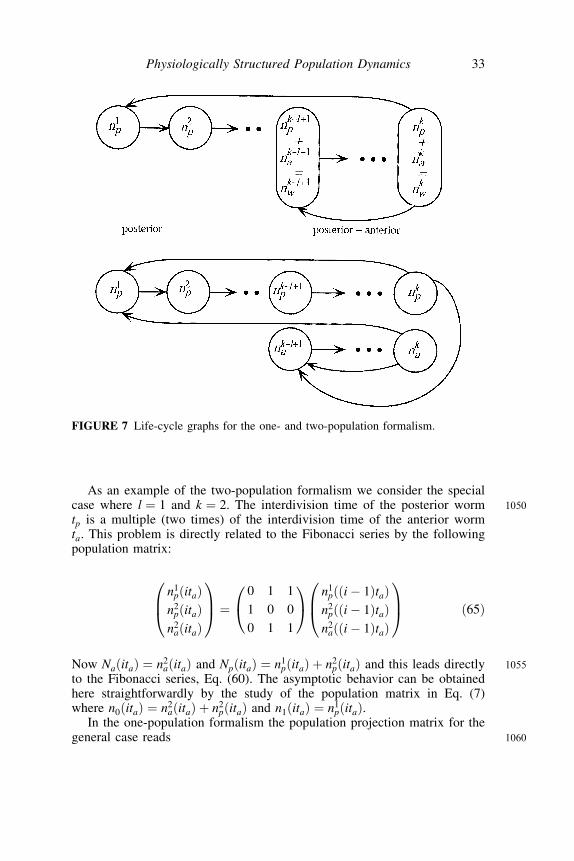
As an example of the two-population formalism we consider the special1050case where l ¼ 1 and k ¼ 2. The interdivision time of the posterior worm

tp is a multiple (two times) of the interdivision time of the anterior wormta. This problem is directly related to the Fibonacci series by the followingpopulation matrix:

n1pðitaÞ

n2pðitaÞ

n2aðitaÞ

0B@

1CA ¼

0 1 1

1 0 0

0 1 1

0@

1A n1

pðði� 1ÞtaÞn2pðði� 1ÞtaÞ

n2aðði� 1ÞtaÞ

0B@

1CA ð65Þ

1055Now NaðitaÞ ¼ n2aðitaÞ and NpðitaÞ ¼ n1

pðitaÞ þ n2pðitaÞ and this leads directly

to the Fibonacci series, Eq. (60). The asymptotic behavior can be obtainedhere straightforwardly by the study of the population matrix in Eq. (7)where n0ðitaÞ ¼ n2

aðitaÞ þ n2pðitaÞ and n1ðitaÞ ¼ n1

pðitaÞ.In the one-population formalism the population projection matrix for the

1060general case reads

FIGURE 7 Life-cycle graphs for the one- and two-population formalism.


nlþ1w ði

ltaÞ

..

.

nkwðil taÞn1pðil taÞ...

nlpðil taÞ

0BBBBBBBBB@

1CCCCCCCCCA

¼

0 � � � 1 0 � � � 1

1 0 � � � � � � 0 0

0 . .. . .

. . .. . .

. ...

..

. . .. . .

. . .. . .

. ...

..

. . .. . .

.1 0 0

0 � � � � � � 0 1 0

0BBBBBBBB@

1CCCCCCCCA

nlþ1w ði�1

ltaÞ

..

.

nkwði�1ltaÞ

n1pði�1

ltaÞ

..

.

nlpði�1ltaÞ

0BBBBBBBBB@

1CCCCCCCCCA

ð66Þ

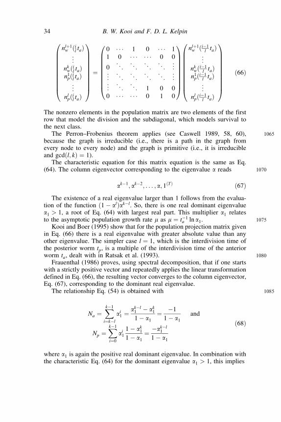
The nonzero elements in the population matrix are two elements of the firstrow that model the division and the subdiagonal, which models survival tothe next class.

1065The Perron–Frobenius theorem applies (see Caswell 1989, 58, 60),because the graph is irreducible (i.e., there is a path in the graph fromevery node to every node) and the graph is primitive (i.e., it is irreducibleand gcdðl; kÞ ¼ 1).

The characteristic equation for this matrix equation is the same as Eq.1070(64). The column eigenvector corresponding to the eigenvalue a reads

ak�1; ak�2; . . . ; a; 1ðTÞ ð67Þ

The existence of a real eigenvalue larger than 1 follows from the evalua-tion of the function ð1 � alÞak�l. So, there is one real dominant eigenvaluea1 > 1, a root of Eq. (64) with largest real part. This multiplier a1 relates

1075to the asymptotic population growth rate m as m ¼ t�1a ln a1.

Kooi and Boer (1995) show that for the population projection matrix givenin Eq. (66) there is a real eigenvalue with greater absolute value than anyother eigenvalue. The simpler case l ¼ 1, which is the interdivision time ofthe posterior worm tp, is a multiple of the interdivision time of the anterior

1080worm ta, dealt with in Ratsak et al. (1993).Frauenthal (1986) proves, using spectral decomposition, that if one starts

with a strictly positive vector and repeatedly applies the linear transformationdefined in Eq. (66), the resulting vector converges to the column eigenvector,Eq. (67), corresponding to the dominant real eigenvalue.

1085The relationship Eq. (54) is obtained with

Na ¼Xk�1

i¼k�l

ai1 ¼ ak�l1 � ak11 � a1

¼ �1

1 � a1

and

Np ¼Xk�1

i¼0

ai11 � ak11 � a1

¼ �ak�l1

1 � a1

ð68Þ

where a1 is again the positive real dominant eigenvalue. In combination withthe characteristic Eq. (64) for the dominant eigenvalue a1 > 1, this implies


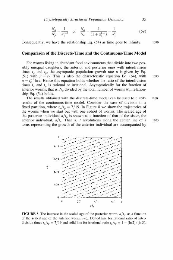
Na

Np

¼ 1

ak�l1

orNa

Nw

¼ 1

ð1 þ ak�l1 Þ ¼

1

ak1ð69Þ

1090Consequently, we have the relationship Eq. (54) as time goes to infinity.

Comparison of the Discrete-Time and the Continuous-Time Model

For worms living in abundant food environments that divide into two pos-sibly unequal daughters, the anterior and posterior ones with interdivisiontimes ta and tp, the asymptotic population growth rate m is given by Eq.

1095(51) with m ¼ c0. This is also the characteristic equation Eq. (64), withm ¼ t�1

a ln a. Hence this equation holds whether the ratio of the interdivisiontimes ta and tp is rational or irrational. Asymptotically for the fraction ofanterior worms, that is, Na divided by the total number of worms Nw, relation-ship Eq. (54) holds.

1100The results obtained with the discrete-time model can be used to clarifyresults of the continuous-time model. Consider the case of division in afixed partition, where ta=tp ¼ 7=19. In Figure 8 we show the trajectories ofthe worms when we start out with one cohort of worms. The scaled age ofthe posterior individual a=tp is shown as a function of that of the sister, the

1105anterior individual, a=ta. That is, 7 revolutions along the center line of atorus representing the growth of the anterior individual are accompanied by

FIGURE 8 The increase in the scaled age of the posterior worm, a=tp, as a function

of the scaled age of the anterior worm, a=ta. Dotted line for rational ratio of inter-

division times ta=tp ¼ 7=19 and solid line for irrational ratio ta=tp ¼ 1� ðln 2Þ=ðln 3Þ.


19 revolutions along the torus. Then the line is continued along the path tra-velled at time 19ta ¼ 7tp ago, showing periodicity. We conclude that the agedistribution does not converge to a stable age distribution. The asymptotic

1110behavior is cyclic.When the ratio of the interdivision times is rational, both the continuous-

time and the discrete-time model apply. We lump the number of individualsinto the life stages introduced earlier, so at time i

lta in life stage j we have,

njpðil taÞ ¼

R j=kvdðj�1Þ=kvd

npðil ta; vÞ dv. The relationship between the growth rate1115m ¼ c0 and the dominant real eigenvalue a1 is: expfmtag ¼ a1.

Convergence to the eigenvector of Eq. (67) means that the distributions ofthe total numbers in the life stage converge. So, within a life stage there is noconvergence, and this is known from the solution of the continuous-timemodel, but the distribution of the total numbers of individuals within the

1120life stages converges to an asymptotic distribution.If the ratio is irrational the dimension of the matrix becomes infinite.

Therefore we study a series ln=kn with kn ! 1 for n ! 1 such that thisseries of rational numbers converges to this irrational number. Then thelength of the life stages converges to zero, and therefore we have effectively

1125convergence to a length distribution. However, the rate of convergencebecomes small because the absolute magnitude of the eigenvalues of thesecond largest one is almost equal to the largest real eigenvalue. Hence,there is convergence, but the rate becomes infinitely small.

In Figure 8 we show the trajectories also for the case1130ta=tp ¼ 1 � ln 2=ðln 3Þ and thus irrational. We do not have periodicity now

as we had before in the rational case (where ta=tp ¼ 7=19 in Figure 8).

CONCLUDING REMARKS

The following observation can be made. First unstructured populationmodels were replaced by simple structured ones where age served as i-

1135state variable. Mathematical techniques were developed to prove existence,permanence, and stability properties of the ultimate age or size distribution.Then the model for the individual underlying the structured population modelbecame more complex for the need to get more biological realism. Laterother i-state variables then age were used and growth depending on the

1140food availability was taken into account, as well as different life stages.Because food is consumed by the population but on the other hand growthdepends on the food availability, generally the food dynamics has to be mod-eled as well. The individual model was described by individual rates in deter-ministic ODEs, and balance laws directly lead to a PDE model formulation at

1145the population level. The mathematical techniques were adapted to cope withthese more complex models and these techniques seemed initially to be suc-cessful. It was possible to take food dynamics into account and to formulate


the interaction via a feedback. However, rather subtle problems arose andvery different mathematical techniques had to be developed to tackle these

1150problems. The step for i-state to p-state is now postponed by dealing withcumulative quantities at the generation level. Stochastic movement throughi-state space can therefore be modeled. This approach is partly based ontechniques from branching processes.

We have mentioned that the growth rate is generally assumed strictly posi-1155tive, gðE; xÞ > 0. Then the direction of the movement along the characteris-

tics neither reverses nor stops. Growth occurs when available internal energyreserves or external food is sufficient to meet maintenance costs which areneeded to maintain the state of living. Consequently, the individual dieswhen gðE; xÞ ¼ 0; see Kooijman (2000), Muller and Nisbet (2000), and

1160Hanegraaf and Kooi (2002). In Kooi and Kooijman (1999) we studied thedynamics of a rotifer population consuming algae in a chemostat. During atransient there was insufficient food to support life of the whole populationfor a relatively short period. When an unstructured model formulation isused where all individuals are identical, death of one member would directly

1165lead to extinction of the whole population. In Kooi and Kooijman (1999) weshowed that when food becomes scarce for a relatively short period, someunlucky individuals with insufficient energy reserves will die, leaving morefood for survivors. Later when food recovered the population recovers aswell and continuously persists.Q2

1170In Gyllenberg et al. (1997) and Persson et al. (1998), populations with bothcontinuous, namely, death, and discrete, namely, reproduction, elements areinvestigated. In Gyllenberg et al. (1997) the dynamics of the population withpulsed reproduction are formulated by a difference equation for one statevariable, namely, the population size. The influence of the environment is

1175taken into account as a density-dependent within-season mortality. This for-mulation is appropriate for simple ecological systems of seasonally breedingpopulations with non-overlapping generations.

In the worms case study, the age at which reproduction occurs determinesthe projection time interval in the Leslie matrix formulation. In Kooi et al.

1180(2001) a similar model formulation was used to analyze the asymptoticdynamics of a waterflea Daphnia magna population with iteroparouspropagation (they reproduce more than once and die immediately after lastreproduction). In that model all individuals are born with a species specificbiovolume and are clones of the parent. In the fixed period between

1185consecutive reproductive events the adult density-dependent mortality is acontinuous process. Natural death occurs when adults reach the speciesspecific maximum age immediately after their last reproductive event.With the Leslie matrix model formulation it was possible to clarify long-term behavior results obtained with numerical integration of the continuous-

1190time model.Cushing (1998) derives the continuous-time PDE model from the discrete-

time matrix model by the limiting process of infinitesimally refining the


classes and the census time interval. This approach shows in the case of age-structured populations the relationship between the McKendrick–von Foer-

1195ster formulation and the Leslie matrix formulation. The relationships betweenthe various discrete- and continuous-time models for the dynamics of PSPmodels are elucidated in de Roos et al. (1992), where a numerical schemefor the solution of physiologically structured populations is derived fromthe Leslie matrix model. In that formulation there is one life stage and there-

1200fore the time step is equal to the fixed time period between two consecutivereproduction events.

Most models presented and analyzed in the literature deal with one iso-lated structured population or one in interaction with unstructured resourcesor predators. The modeling of the trophic interactions is a very important

1205issue when we want to deal with multispecies systems such as communitiesand biosystems, where in the latter case the interaction with a physical envir-onment is explicitly modeled. In principle, each population can be describedby a PDE together with boundary and initial conditions. For several age-structured species, discrete- and continuous-time models are proposed in

1210Cushing (1998). With size-structured populations, modeling interactionsamong species, predator=prey as well as competition interactions are evenmore troublesome. Numerical difficulties with simulations of spatially inho-mogeneous populations with physiologically distinguishable individuals werediscussed in Gurney et al. (2001).

1215In the worms case, the division into an anterior and a posterior worm dis-turbs the equilibrium state of the energy reserves, as the anterior daughtergets a bigger part of the reserves than the posterior one. It is assumed thatthe energy dynamics are fast enough to smooth out the disturbance causedby one division before either of the daughter worms divides. In other

1220words, both daughter worms reach the equilibrium value for energy reservesbefore they in turn divide. This means that all worms have the same i-statewhen they divide. All anterior worms are born identical and therefore thepopulation of anterior worms is concentrated on one line in i-state space.The same is true for the posterior worms, so there are only two possible

1225states of birth.In community ecology, predator=prey interaction, host–parasitoid interac-

tion, inducible defense, competition, mutualism, symbiosis, nutrient recy-cling, invasion, succession, persistence, stability, and so on play animportant role in theory building. These theoretical concepts are used in

1230the study of ecological issues such as the stability–diversity of ecosystemsdebate, the maximum length of food chains, and occurrence of succession.Unstructured ODE population models have been used frequently to addressthese issues whereby the short- and long-term dynamic behavior is studied.

Spatially structured population models (Durrett and Levin 1994, Gurney1235et al. 2001), in which the i-state contains the spatial coordinates of an indivi-

dual, are not discussed in this article but are important in many applications.Structured population models can also be combined with adaptive dynamics


theory to study evolutionary processes. In Claessen and Dieckmann (2002) anage-structured model for predators is used and resource polymorphisms and

1240adaptive speciation are studied. For general structured metapopulationmodels, fitness is defined in Gyllenberg and Metz (2001). The theory ofstructured populations can be applied to metapopulations straightforwardly.There is analogy between local populations or dispersers and individuals,and between metapopulation and population. Birth is now colonization of

1245empty patches by dispersers and death is extinction of a patch population(Gyllenberg and Metz 2001). Thieme (2003) links age-structured modelswith endemic disease models.

There are a limited number of papers dealing with the bifurcation analysesof (PSP) models. We mention the work of Cushing (1989) and Kirkilionis

1250et al. (2001). A computer package BASE (Kirkilionis et al. 2001) is availablefor continuation of steady states of PSP models. For finite dimensional mapsand ODE systems, computer packages are available. We mention AUTO(Doedel et al. 1997) and CONTENT (Kuznetsov and Levitin 1997;Kuznetsov 1998). These packages are in these days heavily used for the

1255numerical bifurcation analysis of unstructured ecosystem (food chain andfood web) models. Although these packages can be used for continuationof bifurcation points of PSP models in principle, this is far from easy inpractise. The availability of a bifurcation package for PSP would stimulatepotential users to apply these models for populations as part of food chain

1260or food web ecosystems.It would be interesting to have the efficiency of the three numerical

methods—the box method, the Lax–Wendroff, and a characteristicsscheme—be compared with that of the EBT method and those basedon upper and lower solutions techniques. Especially when the support

1265of the density function is time dependent, the EBT method works fine,while methods using fixed grids in the i-space are less efficient in thosesituations because this grid has to span the largest support in the time intervalof interest. In the case where the population density vanishes almosteverywhere in the i-state space, integration along the characteristics and

1270the EBT algorithm follows cohorts of individuals through the i-statespace and will work fine. Another possibility is to reduce the dimension ofthe i-state space and to transform to a size or an age-structured populationwith normal population densities using the so-called Murphy trick (Murphy1983).

1275Sometimes mathematical techniques can be used to reduce the PSP modelto equivalent unstructured ODEs or to stage-structured model DDEs (seeNisbet 1997). In Kooi and Kooijman (1999) and Bocharov and Hadeler(2000), conservation laws play an important role in the derivation of thereduced model. When this applies, assumptions often made implicitly

1280during the construction of unstructured models are made explicit and theparameters of the reduced model can be expressed as lumped parametersof the structured model.


The aggregation technique is an analytical tool which has been used forunstructured models and is at present applied to structured population

1285models. Arino et al. (2000) study a model of an age-structured populationwith two time scales. The slow scale corresponds to the demographic processand the fast one describes the migration process between different spatialpatches. Singular perturbation technique is used to show that the solutionsof the system can be approximated by means of the solutions of a simpler

1290(unstructured) problem.In some papers PDE formulations were already used in case studies

addressing the issues mentioned above, but in general this is a tremendoustask. In many studies the PSP model formulation has proven to be essentialfor realistic population modeling; we mention the study of cannibalism.

1295Mathematical and=or biological insight is needed to know beforehandunder which conditions the use of a structured instead of an unstructuredpopulation model is essential to have realism that is required for the purposefor which the mathematical model is used.

REFERENCES

1300Ackleh, A. S., and K. Deng. 2000. A monotone approximation for a nonautonomous size-

structured population model. Q. Appl. Math. 58(2–3):103–113.

Ackleh, A. S., and K. Ito. 1997. An implicit finite difference scheme for the nonlinear size-

structured population model. Numer. Funct. Anal. Optimiz. 18(9–10):865–884.

Angulo, O., and J. C. Lopez-Marcos. 2000. Numerical integration of nonlinear size-structured

1305population equations. Ecol. Model. 133:3–14.

Angulo, O., and J. C. Lopez-Marcos. 2002. Numerical integration of autonomous and non-

autonomous non-linear size-structured population models. Math. Biosci. 177:30–71.

Arino, O., and M. Kimmel. 1989. Asymptotic behavior of a nonlinear functional-integral

equation of cell kinetics with unequal division. J. Math. Biol. 27:341–354.

1310Arino, O., and M. Kimmel. 1993. Comparison of approaches to modelling of cell population

dynamics. SIAM J. Appl. Math. 53(5):1480–1504.

Arino, O., E. Sanchez, R. Bravo de la Parra, and P. Auger. 2000. A singular perturbation in an

age-structured population model. SIAM J. Appl. Math. 60(2):408–436.

Bell, G. I., and E. C. Anderson. 1967. Cell growth and division I. A mathematical model with

1315applications to cell volume distributions in mammalian suspension cultures. Biophys. J.

7:431–444.

Bocharov, G., and K. P. Hadeler. 2000. Structured population models, conservation laws, and

delay equations. J. Diff. Eq. 168:212–237.

Caswell, H. 1989. Matrix population models. Sunderland, MA: Sinauer Associates.

1320Caswell, H. 1997. Matrix methods for population analysis. In Structured-population models in

marine, terrestrial, and freshwater systems, ed. S. Tuljapurkar and H. Caswell, 19–58. New

York: Chapman & Hall.

Caswell, H., and A. M. John. 1992. From the individual to the population in demographic models.

In Individual based approaches and models in ecology, ed. D. L. DeAngelis and L. J. Gross,

132536–61. Springer-Verlag.

Claessen, D., A. M. de Roos, and L. Persson. 2000. Dwarfs and giants: Cannibalism and com-

petition in size-structured populations. Am. Naturalist 155(2):219–237.


Claessen, D., and U. Dieckmann. 2002. Ontogenetic niche shifts and evolutionary branching in

size-structured populations. Evol. Ecol. Res. 4:189–217.1330Cushing, J. M. 1997. Nonlinear matrix equations and population dynamics. In Structured-

population models in marine, terrestrial, and freshwater systems, ed. S. Tuljapurkar and H.

Caswell, 205–243. New York: Chapman & Hall.

Cushing, J. M. 1998. An introduction to structured population dynamics, vol. 71. Philadelphia:

Society for Industrial and Applied Mathematics.

1335DeAngelis, D. L., and L. J. Gross. 1992. Individuals-based models and approaches in ecology.

New York: Chapman & Hall.

de Roos, A. M. 1988. Numerical methods for structured population models: the escalator boxcar

train. Num. Meth. Part. Diff. Eq. 4:173–195.

de Roos, A. M. 1997. A gentle introduction to physiologically structured population models. In:

1340Structured-population models in marine, terrestrial, and freshwater systems, ed. S. Tulja-

purkar and H. Caswell, 119–204. New York: Chapman & Hall.

de Roos, A. M., O. Diekmann, and J. A. J. Metz. 1992. Studying the dynamics of structured

population models: A versatile technique and its application to Daphnia. Am. Naturalist

139(1):123–147.1345Diekmann, O., M. Gyllenberg, H. Huang, M. Kirkilionis, J. A. J. Metz, and H. R. Thieme. 2001.

On the formulation and analysis of general deterministic structured population models. II.

Nonlinear theory. J. Math. Biol. 43(2):157–189.

Diekmann, O., M. Gyllenberg, and J. A. J. Metz. 2003. Steady state analysis of structured

population models. Technical report, preprint.Q31350Diekmann, O., M. Gyllenberg, J. A. J. Metz, and H. R. Thieme. 1998. On the formulation and

analysis of general deterministic structured population models. I. Linear theory. J. Math.

Biol. 36(4):349–388.

Diekmann, O., M. Gyllenberg, H. R. Thieme, and S. M. Verduyn Lunel. 1993. A cell-cycle model

revisited. Technical report, CWI-Report MAM-R9305, Amsterdam, the Netherlands.

1355Diekmann, O., R. M. Nisbet, W. S. C. Gurney, and F. van den Bosch. 1986. Simple mathematical

models for cannibalism: a critique and a new approach. Math. Biosci. 78:21–46.

Doedel, E. J., A. R. Champneys, T. F. Fairgrieve, Y. A. Kuznetsov, B. Sandstede, and X. Wang.

1997. Auto 97: Continuation and bifurcation software for ordinary differential equations.

Technical report, Concordia University, Montreal, Canada.

1360Donachie, W. D. 1968. Relationship between cell size and time of initiation of DNA replication.

Nature 219:1077–1079.Droop, M. R. 1973. Some thoughts in nutrient limitation in algae. J. Phycol. 9:264–272.

Durrett, R., and S. Levin. 1994. The importance of being discrete (and spatial). Theor. Pop. Biol.

46:363–394.1365El Houssif, N. E. 2001. A deterministic size-structured population model for the worm Naidis

elinguis. J. Math. Biol. 42:424–438.

Fairweather, G. and J. C. Lopez-Marcos. 1991. A box method for a nonlinear equation of

population dynamics. IMA J. Num. Anal. 11:525–538.

Feller, W. 1971. An introduction to probability theory and its application, 2nd ed. New York:

1370Wiley.

Frauenthal, J. C. 1986. Analysis of age-structured models. In Mathematical ecology, ed. T. A.

Hallam, and S. A. Levin, 117–147. Springer-Verlag.Q4Fredrickson, A. G. 1991. Segregated, structured, distributed models and their role in microbial

ecology: A case study based on work done on the filter-feeding ciliate Tetrahymena

1375pyriformis. Microb. Ecol. 22:139–159.Fredrickson, A. G., and N. V. Mantzaris. 2002. A new set of population balance equations for

microbial and cell cultures. Chem. Eng. Sci. 57(12):2265–2278.


Gurney, W. S. C., and R. M. Nisbet. 1998. Ecological dynamics. New York: Oxford University

Press.

1380Gurney, W. S. C., D. C. Speirs, S. N. Wood, E. D. Clarke, and M. R. Heath. 2001. Simulating

spatially and physiologically structured populations. J. An. Ecol. 70(6):881–894.

Gurtin, M. E., and R. C. MacCamy. 1974. Nonlinear age-dependent population dynamics. Arch.

Rat. Mech. Anal. 54:281–300.

Gyllenberg, M., I. Hanski, and T. Lindstrom. 1997. Continuous versus discrete single species

1385population models with adjustable reproductive strategies. Bull. Math. Biol. 59:679–705.

Gyllenberg, M., and J. A. J. Metz. 2001. On fitness in structured metapopulations. J. Math. Biol.

43(6):545–560.

Hallam, T. G., R. R. Lassiter, J. Li, and L. A. Suarez. 1990. Modelling individuals employing an

integrated energy response: Application to Daphnia. Ecology 71:938–954.

1390Hanegraaf, P. P. F., and B. W. Kooi. 2002. The dynamics of a tri-trophic food chain with two-

component populations from a biochemical perspective. Ecol. Model. 152(1):47–64.

Hanegraaf, P. P. F., B. W. Kooi, and S. A. L. M. Kooijman. 2000. The role of intracellular

components in food chain dynamics. C. R. Acad. Sci. Ser. III Sci. Vie–Life 323:99–111.

Ito, K., F. Kappel, and G. Peichl. 1991. A fully discretized approximation scheme for size-

1395structured population models. SIAM J. Numer. Anal. 28(4):923–954.

Jagers, P. 1975. Branching processes with biological applications. Probability and mathematical

statistical–applied probability and statistics. New York: Wiley.

Jagers, P. 1991. The growth and stabilization of populations. Stat. Sci. 6:269–283.

Kelpin, F. D. L., M. A. Kirkilionis, and B. W. Kooi. 2000. Numerical methods and parameter

1400estimation of a structured population model with discrete events in the life history. J. Theor.

Biol. 207(2):217–230.

Kirkilionis, M. A., O. Diekmann, B. Lisser, M. Nool, A. M. de Roos, and B. P. Sommeijer. 2001.

Numerical continuation of equilibria of physiologically structured population models I.

Theory. Math. Models Methods Appl. Sci. 11(6):1101–1127.

1405Kooi, B. W., and M. P. Boer. 1995. Discrete and continuous time population models, a com-

parison concerning proliferation by fission. J. Biol. Syst. 3(2):543–558.

Kooi, B. W., T. G. Hallam, F. D. L. Kelpin, C. M. Krohn, and S. A. L. M. Kooijman. 2001.

Iteroparous reproduction strategies and population dynamics. Bull. Math. Biol. 63(4):769–

794.

1410Kooi, B. W., and S. A. L. M. Kooijman. 1999. Discrete event versus continuous approach to

reproduction in structured population dynamics. Theor. Pop. Biol. 56(1):91–105.

Kooijman, S. A. L. M. 2000. Dynamic energy and mass budgets in biological systems.

Cambridge: Cambridge University Press.

Kostova, T. 2002. An explicit third-order numerical method for size-structured population

1415equations. Numer. Methods Partial Differ. Eq. in press.Q5Kot, M. 2001. Elements of mathematical ecology. Cambridge: Cambridge University Press.

Kuznetsov, Y. A. 1998. Elements of applied bifurcation theory, vol. 112 of Applied mathe-

matical sciences, 2nd ed. New York: Springer-Verlag.

Kuznetsov, Y. A., and V. V. Levitin. 1997. CONTENT: Integrated environment for the analysis

1420of dynamical systems. Centrum voor Wiskunde en Informatica (CWI), Amsterdam, the

Netherlands, 1.5 edition.

Lasota, A., and M. C. Mackey. 1984. Globally asymptotic properties of proliferating cell

populations. J. Math. Biol. 19:43–62.

McKendrick, A. G. 1926. Application of mathematics to medical problems. Proc. Edinburgh

1425Math. Soc. 44:98–130.


Metz, J. A. J., and A. M. de Roos. 1992. The role of physiologically structured population models

within a general individual-based modeling perspective. In Individuals-based models and

approaches in ecology, ed. D. L. DeAngelis and L. J. Gross, 88–111. New York: Chapman &

Hall.

1430Metz, J. A. J., and O. Diekmann. 1986. The dynamics of physiologically structured populations,

vol. 68 of Lecture notes in biomathematics. Berlin: Springer-Verlag.

Metz, J. A. J., and O. Diekmann. 1989. Exact finite dimensional representations of models for

physiologically structured populations. I: The abstract foundations of linear chain trickery. In

Differential equations with applications in biology, physics and engineering, ed. J. A.

1435Goldstein, F. Kappel, and W. Schappacher, 269–289. New York: Marcel Dekker.

Milner, F. A., and G. Rabbiolo. 1992. Rapidly converging numerical algorithms for models of

population dynamics. J. Math. Biol. 30(7):733–754.

Muller, E. B., and R. M. Nisbet. 2000. Survival and production in variable resource environ-

ments. Bull. Math. Biol. 62:1163–1189.

1440Murphy, L. F. 1983. A nonlinear growth mechanism in size structured population dynamics.

J. Theor. Biol. 104:493–506.

Nisbet, R. M. 1997. Delay-differential equations for structured populations. In Structured-

population models in marine, terrestrial, and freshwater systems, ed. S. Tuljapurkar and

H. Caswell, 89–118. New York: Chapman & Hall.

1445Persson, L., K. Leonardsson, A. M. de Roos, M. Gyllenberg, and B. Christensen. 1998. Onto-

genetic scaling of foraging rates and the dynamics of a size-structured consumer-resource

model. Theor. Pop. Biol. 54:270–293.

Ramkrishna, D. 2000. Population balances—Theory and applications to particulate systems in

engineering. San Diego: Academic Press.

1450Ratsak, C. H. 2001. Effects of Nais elinguis on the performance of an activated sludge plant.

Hydrobiologia 463:217–222.

Ratsak, C. H., S. A. L. M. Kooijman, and B. W. Kooi. 1993. Modeling the growth of an oli-

gocheate on activated sludge. Water Res. 27(5):739–747.

Richtmeyer, R., and K. Morton. 1967. Difference methods for initial-value problems. New York.Q61455Sharpe, F. R., and A. J. Lotka. 1911. Numerical bifurcation analysis of a tri-trophic food web

with omnivory. Philos. Mag. 21:435–438.

Sinko, J. W., and W. Streifer. 1971. A model for populations reproducing by fission. Ecology

52:330–335.

Sulsky, D. 1993. Numerical solution of structured population models I Age structure. J. Math.

1460Biol. 31:817–839.

Sulsky, D. 1994. Numerical solution of structured population models II Mass structure. J. Math.

Biol. 32:491–514.

Thieme, H. 2003. Mathematics in population biology. Princeton, NJ: Princeton University Press.

Thieme, H. R. 1988. Well-posedness of physiologically structured population models for

1465Daphnia magna. J. Math. Biol. 26:299–317.

Tuljapurkar, S. 1997. Stochastic matrix models. In Structured-population models in marine,

terrestrial, and freshwater systems, ed. S. Tuljapurkar and H. Caswell, 59–87. New York:

Chapman & Hall.

Tyrcha, J. 2001. Age-dependent cell cycle model. J. Theor. Biol. 213(1):89–101.

1470Tyson, J. J., and K. B. Hannsgen. 1985. Global asymptotic stability of the size distribution in

probabilistic models of the cell cycle. J. Math. Biol. 22:61–68.

Tyson, J. J., and K. B. Hannsgen. 1986. Cell growth and division: A deterministic=probabilistic

model of the cell cycle. J. Math. Biol. 23:231–246.


van den Bosch, F., A. M. de Roos, and G. Gabriel. 1988. Cannibalism as a life boat mechanics. J.

1475Math. Biol. 26:619–633.

von Foerster, H. 1959. Some remarks on changing populations. In The kinetics of cellular

proliferation, ed. F. Stohlman. New York: Grune and Stratton.Q7Webb, G. F. 1985. Theory of nonlinear age-dependent population dynamics, vol. 89 of

Monographs and textbooks in pure and applied mathematics. New York: Marcel Dekker.1480


physiologically structured population dynamics: a modeling … · 2003-03-12 · physiologically...

Documents