14 Parametric Instability

14.1 Frequency Matching

The equation of motion for a simple harmonic oscillator x1 is

d2x1

dt2+ ω2

1x1 = 0

where ω1 is the resonant frequency. If it is driven by a time-dependent force

which is proportional to the product of the amplitude E0 of the driver (pump)

and the amplitude x2 of a second oscillator, the equation of motion becomes

d2x1

dt2+ ω2

1x1 = c1x2E0

where c1 is a constant indicating the strength of the coupling. A similar equation

holds for x2

d2x2

dt2+ ω2

2x2 = c2x1E0.

Writing x1 = x1 cosωt, x2 = x2 cosω′t, E0 = E0 cosω0t,

(ω22 − ω′2)x2 cosω

′t = c2E0x1 cosω0t cosωt

= c2E0x11

2cos [(ω0 + ω)t] + cos [(ω0 − ω)t] .

The driving terms on the right can excite oscillators x2 with frequencies

ω′ = ω0 ± ω.

The nonlinear driving terms can cause a frequency shift so ω′ does not need

to be exactly ω2, but only approximately equal to ω2. Furthermore, ω′ can be

complex because there can be damping or growth, so the oscillator x2 has finite

Q and can respond to a range of frequencies.

Let x1 = x1 cosω′′t, x2 = x2 cos[(ω0 ± ω)t]. The equation of motion for x1

becomes

(ω21 − ω′′2)x1 cosω

′′t

= c1E0x21

2(cos [ω0 + (ω0 ± ω)]t+ cos [ω0 − (ω0 ± ω)]t)

= c1E0x21

2cos [(2ω0 ± ω)t] + cosωt .

The driving terms can excite not only the original oscillation x1(ω), but also new

frequencies ω′′ = 2ω0 ±ω. Considering the case |ω0| ≫ |ω1| so that x1(2ω0 ±ω)

can be neglected, coupled equations among x1(ω), x2(ω0 − ω), and x2(ω0 + ω)

are derived

(ω21 − ω2)x1(ω)− c1E0[x2(ω0 − ω) + x2(ω0 + ω)] = 0[ω22 − (ω0 − ω)2

]x2(ω0 − ω)− c2E0(ω0)x1(ω) = 0[

ω22 − (ω0 + ω)2

]x2(ω0 + ω)− c2E0(ω0)x1(ω) = 0.

64

The dispersion relation is given by setting the determinant of the coefficients to

zero, ∣∣∣∣∣∣ω2 − ω2

1 c1E0 c1E0

c2E0 (ω0 − ω)2 − ω22 0

c2E0 0 (ω0 + ω)2 − ω22

∣∣∣∣∣∣ = 0.

For small frequency shifts and small damping or growth rates, ω and ω′ can

be set approximately equal to the undisturbed frequencies ω1 and ω2, so the

frequency matching condition can be written

ω0 ≃ ω2 ± ω1.

When the oscillators are waves in a plasma, ωt should be replaced by ωt− k · r.There is also a wavevector matching condition

k0 ≃ k2 ± k1

describing spatial beating. These conditions can be interpreted as conservations

of energy and momentum.

The simultaneous satisfaction of frequency and wavevector matching condi-

tions is possible only for certain combinations of waves. For one-dimensional

problems, the required relationships can be shown on an ω-k diagram. The fig-

ure shows the dispersion curves of ion acoustic waves (straight lines), electron

plasma waves (wide parabola), and electromagnetic waves (narrow parabola),

and the incident pump wave (ω0) and the two decay waves (ω1 and ω2). The

parallelogram construction ensures that the frequency and wavenumber match-

ing conditions are satisfied simultaneously.

(A) Electron decay instability: A large amplitude electron plasma wave can

decay into a backward moving electron plasma wave and an ion acoustic wave.

The positions of the (ω0, k0) and (ω2, k2) on the electron plasma wave dispersion

curve must be adjusted so that the difference vector (ω1, k1) lies on the ion

acoustic wave dispersion curve.

(B) Parametric decay instability: An incident electromagnetic wave of large

phase velocity (ω0/k0 ≃ c) excites an electron plasma wave and an ion acous-

tic wave moving in opposite directions. Since k0 is small, k1 ≃ −k2 for this

instability.

(C) Parametric backscattering instability: A light wave excites an ion acous-

tic wave and another light wave moving in the opposite direction (stimulated

Brillouin backscattering). A light wave can also excite an electron plasma wave

and a backward moving light wave (stimulated Raman backscattering).

(D) Two-plasmon decay instability: An incident light wave decays into two

oppositely propagating electron plasma waves (plasmons). Frequency matching

can be satisfied only if ω0 ≃ 2ωp (i.e., ne = nc/4 where nc is the critical density

where ω0 = ωp).

14.2 Instability Threshold

Even a small amount of damping (either collisional or collisionless) will prevent

parametric instability unless the pump wave is strong enough. To calculate the

65

Fig. 1. Parallelogram constructions showing the simultaneous matching of

frequency and wavenumber for (A) electron decay instability, (B) parametric

decay instability, (C) stimulated Brillouin backscattering instability, and (D)

two-plasmon decay instability.

threshold, damping rates Γ1 and Γ2 of the oscillators x1 and x2 are introduced,

d2x1

dt2+ ω2

1x1 + 2Γ1dx1

dt= c1x2E0

and similarly for x2. The equations of motion become

(ω21 − ω2 − 2iωΓ1)x1(ω) = c1x2E0

(ω22 − (ω − ω0)

2 − 2i(ω − ω0)Γ2)x2(ω − ω0) = c2x1E0.

Take the case of two waves, i.e., when ω ≃ ω1 and ω0 − ω ≃ ω2 but ω0 + ω is

far enough from ω2 to be nonresonant, i.e., ϵ(ω0 + ω) = 0. Expressing x1, x2

and E0 in terms of their peak amplitudes,

(ω2 − ω21 + 2iωΓ1)

[(ω0 − ω)2 − ω2

2 − 2i(ω0 − ω)Γ2

]=

1

4c1c2E

2

0.

At threshold, ℑ(ω) = 0. The lowest threshold will occur at exact frequency

matching, i.e., ω = ω1, ω0 − ω = ω2, giving

c1c2

(E

2

0

)thresh

= 16ω1ω2Γ1Γ2

The threshold goes to zero with the damping of either wave goes to zero.

14.3 Physical Mechanism

Consider the case of an electromagnetic wave (ω0, k0) driving an electron plasma

wave (ω2, k2) and a low-frequency ion acoustic wave (ω1, k1). Since ω1 is small,

66

ω0 must be close to ωp. The behavior is different for ω0 < ωp (oscillating

two-stream instability) and for ω0 > ωp (parametric decay instability).

Suppose there is a density perturbation in the plasma of the form n1 cos k1x,

which can occur spontaneously as a component of the thermal noise. Let the

pump wave have an electric field xE0 cosω0t and assume there is no DC magnetic

field B0. The pump wave satisfies the dispersion relation ω20 = ω2

p + c2k20, so

k0 ≃ 0 for ω0 ≃ ωp and E0 can be taken to be spatially uniform. If ω0 < ωp,

the electrons will move in the direction opposite to E0 (ions do not move on

this time scale). The density perturbation causes a charge separation. The

electrostatic charge separation creates an electric field E1 which oscillates at

frequency ω0. The ponderomotive force due to the total field is

FNL = −ω2p

ω20

∇⟨(E0 + E1)

2⟩

2ϵ0.

Since E0 is spatially uniform and is much larger than E1, only the cross term

is important

FNL ≃ −ω2p

ω20

∂

∂x

⟨2E0E1⟩2

ϵ0.

Since E1 changes sign with E0, this force does not average to zero. The pon-

deromotive force FNL is zero at the peaks and troughs of n1, but is large where

∇n1 is large. This spatial distribution causes FNL to push electrons from regions

of low density to regions of high density. The resulting DC electrid field drags

the ions and the density perturbation grows. The threshold FNL is the value

just sufficient to overcome the pressure gradient ∇ni1(Ti + Te) which tends to

flatten the density. The density perturbation does not propagate, so ℜω1 = 0.

This is called the oscillating two-stream instability (OTSI), because the sloshing

electrons have a time-averaged distribution function which is double-peaked.

If ω0 > ωp, the directions of ve, E1 and FNL are reversed, and the pondero-

motive force moves ions from dense regions to less dense regions. The density

perturbation would decay if it did not move, but could grow if it travelled at an

appropriate phase velocity, so that the inertial delay between the application of

FNL and the change of ion positions causes the density maxima to move into

the regions into which FNL is pushing the ions. This speed is the ion acoustic

speed cs, as described below. The phase of FNL is exactly the same as the phase

of the electrostatic restoring force in an ion acoustic wave, where the potential

is maximum at the density maximum. Consequently, FNL adds to the restoring

force. The electrons oscillate with large amplitude if the pump wave field is near

the natural frequency of the electron plasma wave, i.e., ω22 = ω2

p + 3k2v2te. The

pump wave cannot have exactly the frequency ω2 because the beat between ω0

and ω2 must be at the ion acoustic wave frequency ω1 = kcs. If this frequency

matching is satisfied, i.e., ω1 = ω0 − ω2, both an ion acoustic wave and an

electron plasma wave are excited at the expense of the pump wave. This is the

mechanism of the parametric decay instability.

67

Fig. 2. Physical mechanism of the oscillating two-stream instability.

14.4 Oscillating Two-Stream Instability

For simplicity, let the temperature Ti and Te and the collision rates νi and νeall vanish. The ion response is described by

Mn0∂vi1∂t

= en0E = FNL

∂ni1

∂t+ n0

∂vi1∂x

= 0.

Since the equilibrium is assumed to be spatially homogeneous, Fourier analysis

in space can be performed to yield

∂2ni1

∂t2+

ik

MFNL = 0.

The electron response is described by

m

(∂ve∂t

+ ve∂

∂xve

)= −e(E0 + E1)

where E1 is related to the density ne1 by Poisson’s equation

ikϵ0E1 = −ene1.

The quantities E1, ve and ne1 have both a high-frequency part, in which the

electrons move independently of the ions, and a low-frequency part, in which the

68

electrons move with the ions. To lowest order, the motion is a high-frequency

one in response to the spatially uniform field E0

∂ve0∂t

= − e

mE0 = − e

mE0 cosω0t.

Linearizing about this oscillating equilibrium,

∂ve1∂t

+ ikve0ve1 = − e

mE1 = − e

m(E1h + E1l)

where the subscripts h and l denote the high- and low-frequency parts. The

first term consists mostly of the high-frequency velocity veh, given by

∂veh∂t

= − e

mE1h =

nehe2

ikϵ0m.

The low-frequency part is

ikve0veh = − e

mEil.

The right-hand side is the ponderomotive force to drive the ion acoustic waves,

resulting from the low-frequency beat between ve0 and veh. The left-hand side

is related to the electrostatic part of the ponderomotive force. The electron

continuity equation is

∂ne1

∂t+ ikve0ne1 + n0ikve1 = 0

The high-frequency part is given by

∂neh

∂t+ ikve0ni1 + ikn0veh = 0

where the middle term produces a high-frequency term only by beating of the

low-frequency density nel = ni1 with ve0. Taking the time derivative, and

neglecting ∂ni1/∂t gives

∂2neh

∂t2+ ω2

pneh =ike

mni1E0.

Taking neh to vary as exp(−iωt),

(ω2p − ω2)neh =

ike

mni1E0.

Combining with Poisson’s equation gives

E1h = − e2

ϵ0m

ni1E0

ω2p − ω2

≃ − e2

ϵ0m

ni1E0

ω2p − ω2

0

.

The ponderomotive force is

FNL ≃ω2p

ω20

e2

m

ikni1

ω2p − ω2

0

⟨E2

0

⟩.

69

Both E1h and FNL change sign with ω2p−ω2

0 . The maximum response will occur

for ω20 ≃ ω2

p. The ion equation can be written

∂2ni1

∂t2≃ e2k2

2Mm

E20ni1

ω2p − ω2

0

.

Since the low-frequency perturbation does not propagate in this instability,

ni1 = ni1 exp γt, where γ is the growth rate, and

γ2 ≃ e2k2

2Mm

E20

ω2p − ω2

0

.

The growth rate γ is real if ω20 < ω2

p. In the presence of finite damping, ω2p −ω2

will have an imaginary part proportional to 2Γ2ωp, where Γ2 is the damping

rate of the electron oscillations. Then

γ ∝ E0√Γ2

.

Far above the threshold, the imaginary part of ω will be dominated by the

growth rate rather than Γ2, so

γ ∝ E2/30 .

To solve the problem exactly, the following pair of equations are solved

∂2ni1

∂t2= − ike

MnehE0

∂2neh

∂t2+ ω2

pneh =ike

mni1E0.

The frequency ω1 vanishes because the ion acoustic speed is zero in the zero-

temperature limit.

14.5 Example of Parametric Decay Instablity

A similar derivation for ω0 > ωp leads to the excitation of an electron plasma

wave and an ion acoustic wave. Frequency spectra of the waves measured in

a plasma are shown in the figure. Below threshold power, the high-frequency

spectrum shows only the pump wave, while the low-frequency spectrum shows

only a small amount of noise. When the pump wave ampltude is increased

above threshold, an ion acoustic wave appears in the low-frequency spectrum,

and an electron plasma wave appears in the high-frequency spectrum as the

lower sideband of the pump wave.

14.6 Parametric Dispersion Relation

Consider a magnetized plasma with B = B0z and the pump wave electric field

E0(x, t) = (E0xx+ E0z

z) cosω0t. The 0-th order Vlasov equation is

∂f0∂t

+ v · ∂

∂xf0 +

q

m

(E0 cosω0t+ v × B

)· ∂

∂vf0 = 0

70

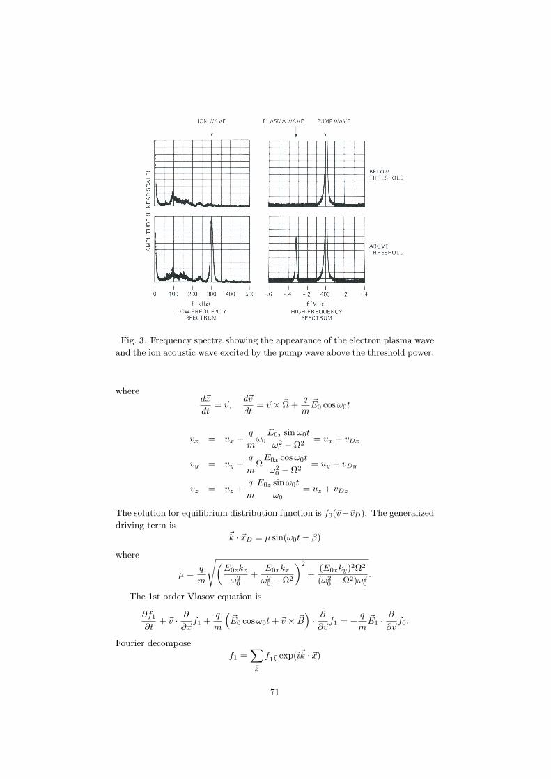
Fig. 3. Frequency spectra showing the appearance of the electron plasma wave

and the ion acoustic wave excited by the pump wave above the threshold power.

wheredx

dt= v,

dv

dt= v × Ω +

q

mE0 cosω0t

vx = ux +q

mω0

E0x sinω0t

ω20 − Ω2

= ux + vDx

vy = uy +q

mΩE0x cosω0t

ω20 − Ω2

= uy + vDy

vz = uz +q

m

E0z sinω0t

ω0= uz + vDz

The solution for equilibrium distribution function is f0(v− vD). The generalized

driving term is

k · xD = µ sin(ω0t− β)

where

µ =q

m

√(E0zkzω20

+E0xkxω20 − Ω2

)2

+(E0xky)2Ω2

(ω20 − Ω2)ω2

0

.

The 1st order Vlasov equation is

∂f1∂t

+ v · ∂

∂xf1 +

q

m

(E0 cosω0t+ v × B

)· ∂

∂vf1 = − q

mE1 ·

∂

∂vf0.

Fourier decompose

f1 =∑k

f1k exp(ik · x)

71

and write

f1k = F (x, u, t) exp(−ik · xD)

∂f1k∂t

=

(∂F

∂t+

∂F

∂u

∂u

∂t− ik

∂xD

∂tF

)exp(−ik · xD)

The 1st order Vlasov equation can be rewritten

∂F

∂t+ u · ∂

∂xF +

q

m(u× B) · ∂

∂uF = − q

m

(E1 ·

∂

∂uf0

)exp(ik · xD).

The solution is

F =q

m

∫ t

−∞dt′

∂φ′(x′, t′)

∂x′ ·(∂f0∂u′

)exp[iµ sin(ω0t

′ − β)].

The exponential term can be expanded in terms of Bessel functions

exp[iµ sin(ω0t′ − β)] =

∞∑−∞

Jn(µ) exp[in(ω0t− β)].

Using∂f0∂u′ = −2u′

v2tF0(u

′2)

andd

dt′=

∂

∂t′+ u′ · ∂

∂x,

F (x, u, t) = f0(u2)

q

m

∫ t

−∞dt′(− 2

v2t

)[(d

dt′− ∂

∂t′

)φ

]exp[iµ sin(ω0t− β)]

which can be Fourier transformed to∫dωF (k, u, ω)ei(k·x−ωt) =

∑n

NnIn

where

Nn = −2q

m

f0(u2)

v2tJn(µ)e

−inβ

In =

∫ t

−∞dt′einω0t

′(

d

dt′− ∂

∂t′

)∫dωφ(k, ω)ei(k·x

′−ωt′).

After some algebra the following expression for F (k, u, ω) can be derived

F (k, u, ω) = − 2q

mv2tf0(u

2)∑n

Jn(µ)e−inβ

1− ω∑l,p

Jl

(k⊥u⊥

Ω

)Jp

(k⊥u⊥

Ω

)ei(l−p)α′

ω − lΩ− k∥uz

φ(k, ω + nω0).

72

The charge density is given by

ρ =

∫ ∞

−∞du∥

∫ 2π

0

dα′∫ ∞

0

u⊥du⊥qF (k, u, ω)

= −2q2n0

mv2⊥

∑n

Jn(µ)e−inβ

[1 +

ω

kzvt

∑l

Il(b)e−bZ(ζl)

]φ(k, ω + nω0)

where

b = k2⊥r2L, ζl =

ω − lΩ

kzvt.

This can be rewritten using the susceptibility χ(ω) as

ρ(ω) = −ϵ0k2∑n

Jn(µ)e−inβχ(ω)φ(ω + nω0)

where

χ(ω, k) =1

k2λ2D

[1 + ζ0

∑l

Il(b)e−bZ(ζl)

].

Poisson’s equation can be expressed as

φk =1

ϵ0k2

∑s

qs

∫d3uF (u)e−ik·vD

The potential can be written as

φ(ω) =1

ϵ0k2

∑s

∑n

Jn(−µs)e−inβρs(ω + nω0).

For µe < 1, Bessel functions can be expanded

J0(µe) = 1− µ2e

4+ · · · ; J±1(µe) = ±µe

2+ · · · .

For ions, µi ≪ 1 and

J0(µi) = 1; J1(µi) = 0.

Consider the case ω0 ≫ ωpi. In this case ion contributions can be ignored

for the sideband ω±, and

ρi(ω) = −ϵ0k2χi(ω)φ(ω)

ρe(ω) = −ϵ0k2χe(ω)

[(1− µ2

4

)φ(ω)− µ

2eiβφ(ω−) +

µ

2e−iβφ(ω+)

]φ(ω) =

1

ϵ0k2

[ρe(ω)

(1− µ2

4

)+

µ

2eiβρe(ω

−)− µ

2e−iβρe(ω

+) + ρi(ω)

]where µ = µe and ω∓ = ω ∓ ω0. Substituting φ(ω) into ρ(ω) gives

ρi = − χi

1 + χi

[(1− µ2

4

)ρe +

µ

2eiβρ−e − µ

2e−iβρ+e

]ρe = − χe

1 + χe

(1− µ2

4

)ρi

ρ−e = − χ−e

1 + χ−e

(µ2e−iβρi

)ρ+e = − χ+

e

1 + χ+e

(−µ

2eiβρi

)73

where χ = χ(ω) and χ± = χ(ω±), and similarly for ρ and ρ±. Substituting into

ρi yields

1 =χi

1 + χi

[(1− µ2

4

)2χe

1 + χe− µ2

4

χ−e

1 + χ−e

+µ2

4

χ+e

1 + χ+e

].

Assuming |ϵ−| ≪ 1 (the lower sideband is resonant) where ϵ = 1+ χe + χi, and

|χe| ≫ 1 (i.e., k2λ2D ≪ 1), the dispersion relation that describes parametric

instability can be written as

ϵ+µ2

4χiχe

(1

ϵ−+

1

ϵ+

)= 0.

14.7 Resonant Decay

Consider the case in which both the low frequency mode (ω1) and the lower

sideband mode (ω2 = ω0 −ω1) are resonant, so that ϵRe(ω1) = 0 and ϵRe(ω2) =

0. The dielectric constant ϵ = ϵRe + iϵIm can be expanded as

ϵ(ω + iγ) = ϵRe(ω) + iγ∂ϵRe(ω)

∂ω+ iϵIm(ω)

= i(γ + Γ)∂ϵRe

∂ω

where

Γ =ϵIm(∂ϵRe

∂ω

)is the damping rate including both collisional damping and collisionless damp-

ing. The dielectric constants at the low frequency and at the lower sideband

are

ϵ(ω1) = i(γ + Γ1)∂ϵRe

∂ω1

ϵ(ω1 − ω0) = −i(γ + Γ2)∂ϵRe

∂ω2.

Ignoring the upper sideband, which is off resonant, the dispersion relation can

be written as

(γ + Γ1)(γ + Γ2) = −µ2

4

χi(ω1)χe(ω1)

∂ϵRe

∂ω1

∂ϵRe

∂ω2

= A2.

The threshold condition is given by setting γ = 0. For resonant decay into

electron plasma wave and ion acoustic wave in the absence of magnetic field,

µ =eE0k

mω20

and

Γ1Γ2 =e2E2

0k2

4m2ω40

(ω2pi/ω

21

) (1/k2λ2

De

)(2/ω2)

(2ω2

pi/ω31

) ≃ ϵ0E20ω1ω2

16n0Te

74

where ω0 ≃ ωpe has been used. For resonant decay into lower hybrid wave and

a low frequency wave (ion acoustic wave or ion cyclotron wave) in the presence

of magnetic field, ωpi < ω0 ≪ ωce in which case the main driving term is the

E × B drift

µ ≃ e

m

E0xkyωceω0

=V kyω0

where V = E0x/B is the E × B velocity. The dispersion relations are given by

ϵRe(ω−) =

k2∥

k2

(1−

ω2pe

ω−2

)+

k2⊥k2

(1−

ω2pe

ω−2 − ω2ce

)

ϵRe(ω) = 1−ω2pi

ω2 − ω2ci

k2⊥k2

−ω2pi

ω2

k2∥

k2+

1

k2λ2De

.

For the lower hybrid wave, the dispersion relation is derived from ϵ(ω−) = 0 as

ω2 = ω2LH

(1 +

k2∥

k2mi

me

); ω2

LH =ω2pi

1 +ω2pe

ω2ce

and 1 + (k2∥/k2)(mi/me) ∼ O(1), so k2∥ ≪ k2. For the ion acoustic wave ωs =

kcs ≫ ωci, and

χi(ω) = −ω2pi

k2c2s= − 1

k2λ2De

.

Therefore,

(γ + Γ1)(γ + Γ2) =

µ2

4

1

(k2λ2De)

2(2

ωsk2λ2De

)2

ω2

(1 +

ω2pe

ω2ce

) =µ2

16

ω2ωs

k2λ2De

(1 +

ω2pe

ω2ce

) .

Taking ky = k⊥ ≃ k for the lower hybrid wave, the threshold condition becomes

Γ1Γ2

ωsωs=

1

16

V 2

c2s

ω2pi

ω20

(1 +

ω2pe

ω2ce

)which can be rewritten

V

cs= 4

ω0

ωLH

√Γ1Γ2

ωsω2.

For typical damping rates of Γ1Γ2/(ωsω2) ≃ 10−2, V/cs ≃ O(1) is required for

instability if ω0/ωLH ≃ 3. Essentially the same result can be obtained for decay

into lower hybrid wave and ion cyclotron wave.

Consider now that there is mismatch so ϵRe = 0, and assume that damping

can be ignored (Γ1 = Γ2 = 0). Defining the frequency mismatch as

δj =ϵRe(∂ϵRe

∂ωj

) ; j = 1, 2

75

the growth rate can be expressed as

γ =−i(δ1 + δ2)±

√4A2 − (δ1 − δ2)2

2

indicating that the frequency mismatch acts like damping to introduces an ef-

fective threshold.

14.8 Decay into Quasi-Modes

Quasi-modes do not exist naturally without the nonlinear drive. The low fre-

quency mode (quasi-mode) does not satisfy the linear dispersion relation, so

ϵRe(ω) = 0, but the lower sideband is assumed resonant ϵRe(ω−) = 0 while the

upper sideband is nonresonant ϵRe(ω+) = 0. For the quasi-mode |χi(ω)| ≫ 1

and |χi(ω)| ≫ |χe(ω)|, so ϵ(ω) ≃ χi(ω). The parametric dispersion relation is

then

1 +µ2

4

χe(ω)

ϵRe(ω2)− i(γ + Γ2)∂ϵRe

∂ω2

= 0.

Consider the case in which the low frequency quasi-mode is strongly Landau

damped,

ϵ(ω1) = ϵRe(ω1) + iϵIm(ω1) ≃ ϵRe(ω1) + iχeIm(ω1).

The growth rate can be obtained by balancing the imaginary parts

γ = −Γ2 +µ2

4

χeIm(ω1)(∂ϵRe

∂ω2

)where

χeIm =1

k2λ2De

ζℑZ(ζ).

Resonant decay assumes that the low frequency mode is weakly damped.

In the example of decay into lower hybrid wave and ion acoustic wave, as the

pump wave frequency approaches ωLH , this assumption breaks down since

ωs

k∥vte=

kcsk∥vte

≃ k

k∥

√me

mi.

For the lower hybrid wave (k2∥/k2)(mi/me) ∼ O(1), so ω1/(k∥vte) ≃ O(1). In

this case ωIm ≃ ωRe since ℑ[ζZ(ζ)] ≃ O(1) and the low frequency mode is

heavily electron Landau damped, indicating that the low frequency mode is a

quasi-mode, not a resonant mode. This is called the electron quasi-mode. The

most unstable situation occurs when χeIm maximizes at 0.76/(k2λ2De),

γ + Γ2 =V 2k2

8ω20

ω2

1 +ω2pe

ω2ce

0.76

k2λ2De

=V 2

8c2s0.76ω2

ω2LH

ω20

.

76

The threshold is given by setting γ = 0, so

V 2

c2s≃ 10Γ2

ω2

ω20

ω2LH

.

Note that the growth rate for quasi-mode decay increases like γ ∝ E20 compared

to γ ∝ E0 for resonant decay. Although the threshold is higher than that for

resonant decay, once the threshold is exceeded quasi-mode decay grows faster.

When the low frequency mode is strongly ion-cyclotron damped (ω1 = nωci),

it is called the ion-cyclotron quasi-mode. In this case the frequency spectrum

typically exhibits many peaks at harmonics of the ion-cyclotron frequency.

When the low frequency mode is strongly ion Landau damped (ω1 = k∥cs ≃k∥vti), it is called the ion-acoustic quasi-mode. In this case the sideband fre-

quency is usually not separated from the pump wave, and appears like frequency

broadening.

77