playing othello by deep learning neural networki.cs.hku.hk/fyp/2016/report/final_report/yip tsz...
TRANSCRIPT

The University of Hong Kong
Department of Computer Science
Final Year Project
Playing Othello byDeep Learning Neural Network
Yip Tsz Kwan
in collabortion with CHAN Lok Wang
Supervised by
Dr. K.P. Chan
16 April 2017


Abstract
Board game implementation has long been a way of showing the ability of AI. Among differentboard games, Othello is one of the popular subjects due to its simple rules and well-definedstrategic concepts. Today, the majority of the Othello programmes at a master level stillrequire expert knowledge in their development. To choose the best next move from a givenboard state, the computer Othello searches through the game tree and return move (as atree node) with the optimal value. Though, the evaluation function used to assign value tothe nodes in a game tree relies on the feature studies by human experts.
This project aims to use a machine learning technique, deep learning neural network, to playOthello without any human logic. This implies the computer Othello has to learn the gamefrom scratch through the past gameplays. The targeted winning rate of the computer Othellodeveloped is 50% when playing against a moderate opponent, and 35% when playing againsta strong opponent.
With different models being implemented and tested, the model with 3 convolutional layersand 3 pooling layers gave the best performance. It has a fair winning chance when playingagainst a moderate opponent, though its performance against a strong opponent was not asdesirable.

Acknowledgments
I would like to thank my supervisor, Dr. K.P. Chan, for his continuous guidance and supportthroughout the project, and the second examiner, Dr. Chung Ronald.
I would also like to express my sincere gratitude to my teammate, Chan Lok Wang, Anna,for her effort and significant contribution to this project.
Thank you Ng Argens and Yu Kuai for sharing their data for the neural network modeltraining, and Eric P. Nichols for making the source code of the Othello programme publiclyavailable.
Last but not least, I would like to thank all the staff of the Department of Computer Sciencefor their teaching and support throughout the years.
ii

To my parents and sisters

Contents
Abstract . . . . . . . . . . . . . . . . . . . . . . . . . . . . . . . . . . . . . . . . . . i
Acknowledgements . . . . . . . . . . . . . . . . . . . . . . . . . . . . . . . . . . . . ii
List of Figures . . . . . . . . . . . . . . . . . . . . . . . . . . . . . . . . . . . . . . vi
List of Tables . . . . . . . . . . . . . . . . . . . . . . . . . . . . . . . . . . . . . . . vii
1 Introduction 1
1.1 Background . . . . . . . . . . . . . . . . . . . . . . . . . . . . . . . . . . . . . 1
1.2 Project Objectives . . . . . . . . . . . . . . . . . . . . . . . . . . . . . . . . . 3
1.3 Organization of the Report . . . . . . . . . . . . . . . . . . . . . . . . . . . . 3
2 Existing Work 4
3 Methodology 6
3.1 Training Data Collection and Processing . . . . . . . . . . . . . . . . . . . . . 6
3.1.1 Training Data Collection . . . . . . . . . . . . . . . . . . . . . . . . . 6
3.1.2 Training Data Processing . . . . . . . . . . . . . . . . . . . . . . . . . 7
3.2 Implementation Language . . . . . . . . . . . . . . . . . . . . . . . . . . . . . 8
3.3 Neural Network Design and Implementation . . . . . . . . . . . . . . . . . . . 9
3.3.1 Overview of Neural Network . . . . . . . . . . . . . . . . . . . . . . . 9
3.3.2 Neural Network Design . . . . . . . . . . . . . . . . . . . . . . . . . . 10
3.4 Decision-making Algorithms . . . . . . . . . . . . . . . . . . . . . . . . . . . . 12
3.4.1 Minimax Algorithm . . . . . . . . . . . . . . . . . . . . . . . . . . . . 12
3.4.2 Alpha-beta Pruning . . . . . . . . . . . . . . . . . . . . . . . . . . . . 13
3.5 Testing . . . . . . . . . . . . . . . . . . . . . . . . . . . . . . . . . . . . . . . 14
iv

4 Division of Work 16
5 Results and Discussion 17
5.1 Neural network model 1: 5 Convolutional Layers and 3 Pooling Layers . . . . 17
5.1.1 Parameters specifications . . . . . . . . . . . . . . . . . . . . . . . . . 18
5.1.2 Training Result and Analysis - Data Accuracy . . . . . . . . . . . . . 18
5.1.3 Training Result and Analysis - Testing against a Computer Othello . . 19
5.2 Neural network model 2: 3 Convolutional Layers and 1 Dropout Layer . . . . 20
5.2.1 Parameters specifications . . . . . . . . . . . . . . . . . . . . . . . . . 21
5.2.2 Training Result and Analysis - Data Accuracy . . . . . . . . . . . . . 21
5.2.3 Training Result and Analysis - Testing against a Computer Othello . . 24
5.3 Neural network model 2: 3 Convolutional Layers and 3 Pooling Layer . . . . 25
5.3.1 Parameters specifications . . . . . . . . . . . . . . . . . . . . . . . . . 25
5.3.2 Training Result and Analysis - Data Accuracy . . . . . . . . . . . . . 25
5.3.3 Training Result and Analysis - Testing against a Computer Othello . . 27
6 Conclusion and Future Research 29
6.1 Conclusions . . . . . . . . . . . . . . . . . . . . . . . . . . . . . . . . . . . . . 29
6.2 Future Research Directions . . . . . . . . . . . . . . . . . . . . . . . . . . . . 29
References . . . . . . . . . . . . . . . . . . . . . . . . . . . . . . . . . . . . . . . . . 29
Appendix 32
A The game of Othello 32
v

List of Figures
2.1 The initial board state of Othello . . . . . . . . . . . . . . . . . . . . . . . . . 4
3.1 A board state and its corresponding representations. . . . . . . . . . . . . . . 7
3.2 An example of a neural network with three layers. . . . . . . . . . . . . . . . 9
3.3 A classical CNN architecture . . . . . . . . . . . . . . . . . . . . . . . . . . . 10
3.4 Demonstration of the minimax algorithm . . . . . . . . . . . . . . . . . . . . 12
5.1 Data accuracy of neural network model 1-1 . . . . . . . . . . . . . . . . . . . 18
5.2 Data accuracy of neural network model 1-2 . . . . . . . . . . . . . . . . . . . 19
5.3 Test Result of neural network model 1-1 . . . . . . . . . . . . . . . . . . . . . 20
5.4 Test result of neural network model 1-2 . . . . . . . . . . . . . . . . . . . . . 20
5.5 Data accuracy of neural network model 2-1 . . . . . . . . . . . . . . . . . . . 22
5.6 Data accuracy of the first 30 moves in neural network model 2-2 . . . . . . . 23
5.7 Data accuracy of the last 30 moves in neural network model 2-2 . . . . . . . . 23
5.8 Test Result of neural network model 2-1 . . . . . . . . . . . . . . . . . . . . . 24
5.9 Test result of neural network model 2-2 . . . . . . . . . . . . . . . . . . . . . 24
5.10 Data accuracy of neural network model 3-1 . . . . . . . . . . . . . . . . . . . 26
5.11 Data accuracy of neural network model 3-2 . . . . . . . . . . . . . . . . . . . 27
5.12 Test Result of neural network model 3-1 . . . . . . . . . . . . . . . . . . . . . 28
5.13 Test result of neural network model 3-2 . . . . . . . . . . . . . . . . . . . . . 28
A.1 Initial board position of Othello . . . . . . . . . . . . . . . . . . . . . . . . . . 33
A.2 A legal move in the game Othello. . . . . . . . . . . . . . . . . . . . . . . . . 33
vi

List of Tables
3.1 Cell representation scheme . . . . . . . . . . . . . . . . . . . . . . . . . . . . . 7
3.2 Level of difficulties of The Othello . . . . . . . . . . . . . . . . . . . . . . . . 15
5.1 Parameters of two trained models . . . . . . . . . . . . . . . . . . . . . . . . 17
5.2 Parameters of two trained models . . . . . . . . . . . . . . . . . . . . . . . . 18
5.3 Parameters of two trained models . . . . . . . . . . . . . . . . . . . . . . . . 21
5.4 Parameters of two trained models . . . . . . . . . . . . . . . . . . . . . . . . 26
vii

Chapter 1
Introduction
1.1 Background
In March 2016, computer programme AlphaGo shocked the world by winning 4 out of 5games against the professional Go player, Lee Sedol, one of the best players at Go. Therapid improvement in a chess game engine came at a surprise to many experts of artificialintelligence, who once thought computer beating a human champion of Go would not happenin the next decade. [1] As AlphaGo outperformed a human champion of Go, it drove us toinvestigate the possibility of applying the techniques used by AlphaGo to play another boardgame - Othello.
Othello is another board game played by two players, who take turns to place their discs,in black and white, on the game board. Due to the smaller board size of and limited movesin each round of the game, Othello is considered as an easier game for AI to play. Thedevelopment of Computer Othello is quite mature. In 1997, Logistello won against a humanchampion by 6-0 games.
Game-playing has long been an interest in artificial intelligence due to its complexity. Thecomputer player is required to evaluate the current board state and select the best next moveconstantly throughout the game, as if a human player does. Hence, it becomes a way to testthe ability of the computer and to evaluate how well a computer can perform against human.
Traditionally, a computer plays a board game by the searching through the game tree, atree that contains all the possible moves with the corresponding weights. Due to the limitedstorage capacity of a computer and the huge computational complexity of the game treesearch, for most of the games, it is impossible get the weights of each next state by propagatingthe final result of the leaf nodes back to the upper layers. As a result, an evaluation functionis used to assign the weight to the possible moves in a tree. [2] The problem of how accuratean evaluation function can assign the weight to the given board configuration arises and hasbecome the study focus for developing a game engine. The major technique used to generatean evaluation function in AlphaGo is by deep learning neural network, a machine learningalgorithm.
Inspired by the human brain, neural network is a way of information processing. Severallayers of nodes in the neural network are connected together. As the system is trained,the connections between the nodes will change accordingly. A large amount of trainingdata is used to fine-tune the connection during the training process so that the network can
1

produce a specific output corresponding to the given input. A deep learning neural networkis a network with many hidden layers. [3] More features can be captured and studied ineach hidden layer to increase the accuracy of the final result. A combination of the deeplearning neural network and convolutional neural network(CNN), which explicitly assumesthe training data as images, is used in this project.
This project aims to demonstrate how powerful deep learning neural network can be forgameplay by developing a computer Othello with board size being 8x8 using deep learningneural network. Othello is chosen as the size and the complexity of this game is suitable for aone-year long project with limited resources. The technique of deep learning neural networkcan also be applied to this game. More information on the rules of Othello can be foundin Appendix I. When both players play the game perfectly, it appears that the game willvery likely end with a draw. [4] Therefore, the targeted winning rate when playing against amoderate opponent is 50% and that when playing against a strong opponent is 35%.
In general, there are two main types of neural networks for the game Othello - the policynetwork and the value network. The policy network outputs a probability distribution overthe possible moves, while the value network evaluate the winning probability of the givenboard state.[5] As the possible moves at each round of the game is limited, the implementationof the policy network is of a lower priority. Due to the time limitation, only the value networkwas implemented and tested for the computer Othello.
The main contribution of this project is to provide an alternative to build an evaluationfunction for a computer Othello without any human logic. While different algorithms ofmachine learning, such as reinforcement learning, have been used to train a computer Othello,at the time when this project was proposed, no research on training a computer Othello bydeep learning neural network has been made available. Hence, the result and analysis ofthis project can serve as a reference for future development of computer Othello using deeplearning neural network.
2

1.2 Project Objectives
The objective of this project is to develop a desktop computer Othello with the technique ofdeep learning neural network and the following attributes:
• The game board configuration size being 8 x 8;
• A winning rate of 50% when playing against a moderate (computer) opponent;
• A winning rate of 35% when playing again a strong (computer) opponent; and
• A user-friendly user interface (UI) for easy playing
While the ultimate outcome is to deliver the programme with the specification above, the keyof this project is to construct the evaluation function of the programme by the programmeitself via the value network without any human logic.
1.3 Organization of the Report
The organization of this report is as follows:
Chapter 2 This Chapter describes the detailed background of the project, including theexisting solution and the technical gap.
Chapter 3 This Chapter explains the detailed design and implementation of the project,including the training data collection, the algorithm used, neural network design andgame engine implementation.
Chapter 4 This Chaper presents the work division among the team members
Chapter 5 This Chapter presents, analyzes and discusses the results of different neuralnetworks trained.
Chapter 6 This Chapter concludes the project, and suggests potential areas of improvementbased on the current work, as well as future research directions.
3

Chapter 2
Existing Work
Othello is a strategy game played by two players in black and white discs. While many boardsizes are available for this game, the standard board size is 8-squares-by-8-squares. With theinitial board state shown in Figure 2.1, the black and white players take turn to make a movewith the black player starting playing first. The black player makes the first move by playinga black disc on an empty square adjacent to his opponents disc. As shown in Figure 2.1, thevalid move of the black player at this state are C4, D3, E6, and F5. Opponents discs that aresandwiched between the newly placed disc and another disc of the same color along a linein any direction (horizontal, vertical, or diagonal) are flipped to match with the color of thenewly made move. If a player has no valid move, the player passes. The game ends when noplayers can make a valid move. The player with the most discs of his colours wins the game,while his opponent loses the game. When the number of black and white discs are equal, adraw is declared.
Figure 2.1: The initial board state of Othello
Note that as there are finitely many agents, actions and states in Othello, Othello is a finitegame. Given a particular instance of an Othello game, since every agents are clear about thecurrent state of the game, all the possible action and what they should do, this game is ofperfect information. Finally, since the gain of a player in each flip equals to the loss of hisopponent, the total payoff throughout the game is constant. Hence, Othello is a zero-sumgame. These properties are critical for implementing the game tree and the search algorithms.
Different computer Othello’s have been developed to demonstrate the strength of AI through-out the years. In 1980, the Othello program Moor, written by Mike Reeve and David Levyl,won one game in a six-game match against world champion Hiroshi Inoue. It was the firsttime a computer Othello could win a game of Othello against a human world champion. 17years later, in 1997, Logistello won all the games in a six-game match against world cham-
4

pion Takeshi Murakami. It proves that a computer Othello can play Othello better than anyhuman players.[6]
To train the programme Logistello, features of discs at the end of the game were studied andmapped by logistic regression. Millions of training positions were thoroughly studied andlabeled with a true minimax value or an approximation. A large sparse linear regression wasused to assign values to pattern configurations at 13 game stages, with each being definedby the number of discs on the board.[7] It takes feature correlations into accounts whendoing the value assignment, which was not achieved by previous computer Othello’s and wasconsidered as the reason of its success.
Despite the success of the current computer Othello’s, one may still think if it is possiblefor a computer to learn the game all by itself, i.e. the ability of the computer Othello todetermine the value of a board state from scratch by itself without any human knowledgeof the game being involved. This is where machine learning can be applied to the computerOthello training.
There were attempts to train the computer Othello by neural network over the years, whichcan be divided into two categories in terms of data treatment. The first type is learn thegame in the process of game play. In the study done by M. van der Ree in 2013[8], differentstrategies in reinforcement learning were implemented, including TD-learning and Q-learning.The computer Othello was trained to learn from three types of opponents, including fromself-play, from a fixed opponent, and the fixed opponent’s move. A good performance in thetest was achieved.
The second type of computer Othello training is by learning from the previous game. Thistype of training often involves Othello heuristics. Favourable moves, for example, move at thecorner, were often given a higher score during data processing for later training. K. A. Cherrytrained a computer Othello using neural network with genetic algorithm. During the dataprocessing, he assigned higher score to the advantageous moves. [9] While this approach gavea better performance for training, human knowledge was involved in the training process.
The problem of how well a computer Othello can learn the game without any human logicarises. With the success of AlphaGo, it is worth investigating how well deep learning neuralnetwork may be a good way to train a computer Othello without any human knowledge ofthe game.
5

Chapter 3
Methodology
3.1 Training Data Collection and Processing
To facilitate the training process, 885 sets of game move records were collected throughoutthe project. 172812 different board configurations were obtained from the game move recordsand used in the neural network training. The value of each board configuration were assignedin two ways total sum and averaging.
3.1.1 Training Data Collection
100 sets of game move records were collected at the initial stage of the project. 50 sets ofthose records were obtained from the games played by human against the Android and iOSapplication The Othello with different levels of difficulty. Another 50 sets of the recordswere obtained from the games played by the application against itself with different levels ofdifficulty. Together with another 100 sets of game move records provided by Ng Argens andYu Kuai, 200 sets of game move records were first being processed and used in the initialstage of the neural network training.
During the training process, another 685 sets of game move records were collected from thegames played in the Othello WorldCup 2013 and World Othello Championship 2016 in hopeto resolve the overfitting problem. These game move records, with relatively higher reliability,were processed and used in the later neural network trainings.
For each Othello game, the moves are recorded sequentially in the same file with the formatof each move being specified as
cixiyi
where ci, an integer with two possible values 0 and 1, represents the color of the disc inthe ith move , with 0 being white and 1 being black. xi and yi, where 0xi, yi7 are twointegers representing the x-coordinate and the y-coordinate of the disc position in the ith
move respectively.
6

3.1.2 Training Data Processing
A programme was written to translate each move in a game move record to the correspondingboard state. Each board state is represented by a string of 64 characters (without border) ora string of 100 characters (with border). The representation schemes are shown as the tablebelow:
Value Scheme 1 Scheme 2 Scheme 3
0 An empty cell Empty cell Border
1 Cell occupied by a white disc Cell occupied by a white disc Cell occupied by a white disc
2 Cell occupied by a black disc Cell occupied by a black disc Cell occupied by a black disc
3 N/A Border Empty cell
Table 3.1: Cell representation scheme
Scheme 1 is used to represent the board state without the any border consideration, whileScheme 2 and Scheme 3 are used to represent the board state with the consideration of border.Figure 3.1 shows a board state of one game. Using Scheme 1, its corresponding board staterepresentation is "0000000000000000000000000022200000021000000000000000000000000000", while us-ing Scheme 2 and Scheme 3, its corresponding board state presentations are"3333333333300000000330000000033000000003300222000330002100033000000003300000000330000000033333333333"
and"0000000000033333333003333333300333333330033222333003332133300333333330033333333003333333300000000000"
respectively.
Figure 3.1: A board state and its corresponding representations.
After converting all the moves in the game move records to their corresponding board states,each board state will be assigned a value. If the white player wins the game, +1 score willbe added to all the board states in that game record. If the white player loses the game,-1 score will be added to all the board states in that game record. If it is a draw, 0 will beadded to all the board states in that game record. Due to the symmetric property of theboard, while assigning a value to each board state in the game, a value is also assigned to allits corresponding rotation board state.
A programme is written to do the value assignment. It opens each file containing all theboard states of the game and read the final result of the game from the last line. Then, foreach board state in the file, the programme looks up the board state and all its rotation fromthe vector which storing all the board states. If the board state read from the file is found inthe vector, the value of the board state will be updated according to the final result of thatgame, i.e. either +1, -1, or 0 will be added to the existing board value. If the board state is
7

not found in the vector, it will be pushed back to the vector with the initial value being theresult of the game. Below is the pseudo-code of the board value assignments:
Data: number of gamesResult: a vector containing the board states in all the game move records and their
corresponding valuevector(string, int) boards;i = 0 ;while i <number of games do
read result of the game;if result = white wins then
value = 1 ;else if result = white loses then
value = -1 ;else
value = 0 ;endwhile not the last line of the file do
for each rotation of the board state dolook up the board state from boards;if found then
boards.value += value ;else
boards.push back(state, value) ;end
end
end++i ;
endAlgorithm 1: Board state value assignment
Two sets of output files are generated from the above algorithm for neural network training- one with all the board states and their corresponding total score, and another with all theboard states and their corresponding weighted score, where the weighted score of each boardstate is calculated by weighted score = total score
numberofgames .
3.2 Implementation Language
The main implementation language for this project should support both functional designand UI design. For functional design, it must support neural networking training. Python ischosen as the programming language for this reason.
Python, first released in 1991, is a general-purposed, interpreted, dynamic programminglanguage. Python is among the programming languages who are used for data processing.More importantly, there are many libraries in Python that support deep learning, for instance,Caffe, TensorFlow, and Theano. In particular, Keras was chosen for implementation.
Keras, written in Python, is a high-level neural networks API. It can run on top of eitherTensorFlow or Theano, which are both popular deep learning libraries. In addition, the user-
8
friendliness, modularity and extensibility of Keras allow easy and fast prototyping [10]. Thesimple APIs enable us to observe the neural network design directly from the source code,which helps the implementation and modification of the neural network. In this project,Theano was chosen as the backend library. Theano is among the oldest and the most stabledeep learning library. [11]It is also widely used in academic research. With Keras as wrapper,Theano performs better in terms of speed, classification accuracy and source lines of code fordeep learning. [12]
3.3 Neural Network Design and Implementation
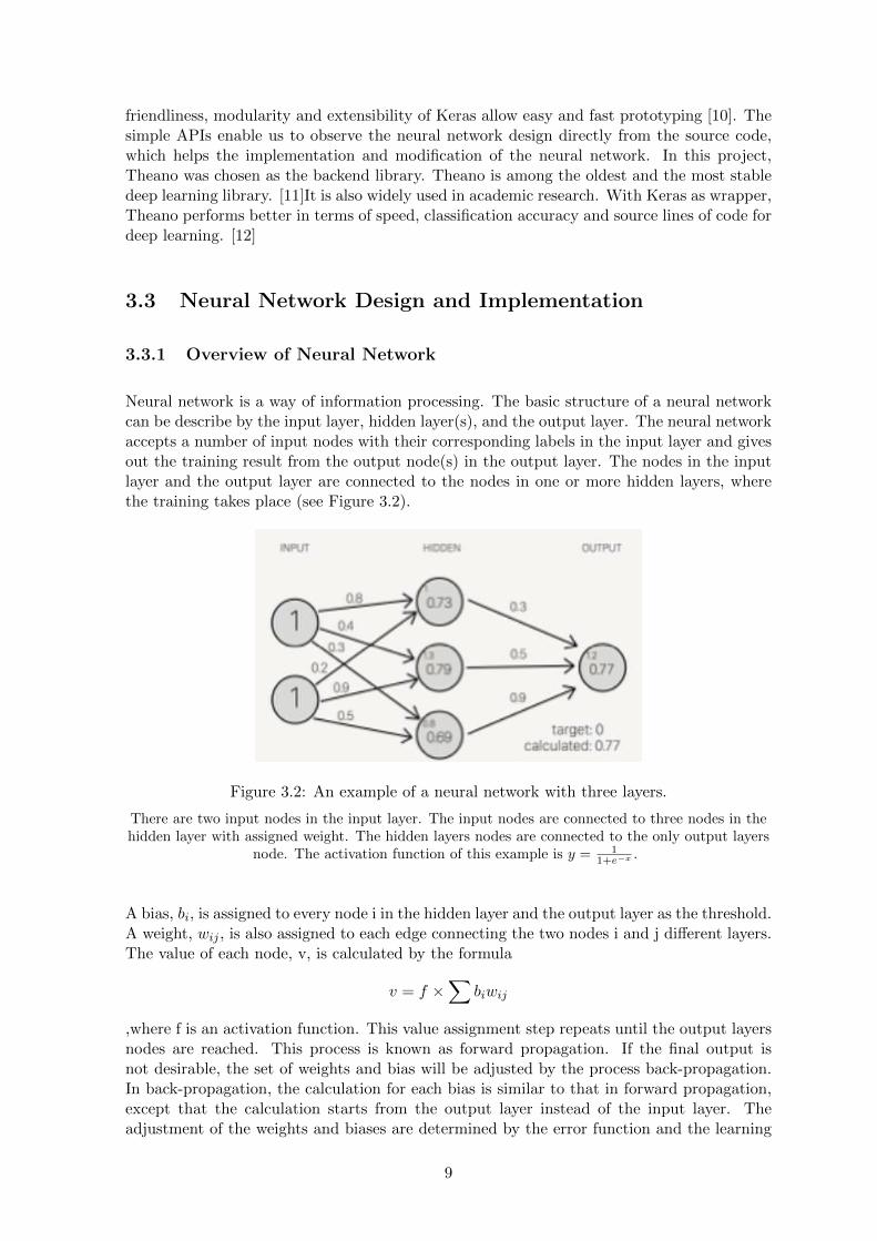
3.3.1 Overview of Neural Network
Neural network is a way of information processing. The basic structure of a neural networkcan be describe by the input layer, hidden layer(s), and the output layer. The neural networkaccepts a number of input nodes with their corresponding labels in the input layer and givesout the training result from the output node(s) in the output layer. The nodes in the inputlayer and the output layer are connected to the nodes in one or more hidden layers, wherethe training takes place (see Figure 3.2).
Figure 3.2: An example of a neural network with three layers.
There are two input nodes in the input layer. The input nodes are connected to three nodes in thehidden layer with assigned weight. The hidden layers nodes are connected to the only output layers
node. The activation function of this example is y = 11+e−x .
A bias, bi, is assigned to every node i in the hidden layer and the output layer as the threshold.A weight, wij , is also assigned to each edge connecting the two nodes i and j different layers.The value of each node, v, is calculated by the formula
v = f ×∑
biwij
,where f is an activation function. This value assignment step repeats until the output layersnodes are reached. This process is known as forward propagation. If the final output isnot desirable, the set of weights and bias will be adjusted by the process back-propagation.In back-propagation, the calculation for each bias is similar to that in forward propagation,except that the calculation starts from the output layer instead of the input layer. Theadjustment of the weights and biases are determined by the error function and the learning
9

rate of the neural network.
A deep learning neural network is neural network with more than one hidden layer. Inparticular, a convolutional neural network was implemented in this project.
Figure 3.3: A classical CNN architecture
The input layer takes the input training data and its corresponding labels. The first convolutionallayer captures the lower-level features of the image and generates an activation map according to thefilters defined. Then an elementwise activation function is applied on the activation map, and passesthe result to the next convolutional layer. Pooling layers are added in between to reduce the network
complexity, including the number of parameters and computation time. Finally, a fully-connectedlayer is added at the end to combine the previous training result and give an output of the training.
A CNN is a neural network that consists of some convolutional layers, which helps reducethe number of parameters, and hence reduce the overfitting problem. [13] It also explicitlyassumes taking 2D structure of an input image in the input layer, which is favourable forprocessing the input training data, i.e. board states, in this project. Figure 3.3 shows aclassical CNN architecture. Similar to all the neural network, a CNN has the input layeras its first layer. Right after the input layer is a convolutional layer, which is essential tocapture lower features of the image. Then the activation function and pooling layer(s) willbe applied together with the convolutional layer has the hidden layers of the deep learningneural network. The CNN ends with a fully connected layer, which gives the final output ofthe training. Below is a detailed description of the layers in a convolutional neural network:
Input layer It takes the input data and its corresponding labels for the neural networktraining..
Convolutional layer It is the first layer after the input layer. A number of n-by-n filtersare applied and adjusted to extract the most useful information for the training inthis layer. After filtering on the input, a activation map (also known as a featuremap) is obtained. On the next convolutional layer, another set of filters are applied onthe activation map obtained from the previous convolutional layer. This results in anactivation map that represents higher level features.
Pooling Layer It is commonly added between successive convolutional layer to reduce thespatial size of the representation. This can reduce the complexity of the neural network.
Fully-connected layer It is fully-connected with the previous layer. Weighted sum of thenode(s) are computed by matrix multiplication in this layer.
Dropout layer This layer drops some units and their connections from the neural networkduring the training to prevent overfitting.
3.3.2 Neural Network Design
Different neural network models were implemented and tested throughout the project. Thesemodels can be classified into 3 designs according to their network architecture. The followingsubsections describes their neural network architecture.
10

3.3.2.1 Neural Network Design 1: 5 Convolutional Layers and 3 Pooling Layers
This model design is the most complex among all the three designs. A larger model with moreconvolutional layers and pooling layers is first designed and trained in the hope of capturingmore features during the training. 5 convolutional layers in total are added to the neuralnetwork, with a pooling layer added after every two successive convolutional layers and afterthe last convolutional layer. The neural network is flattened at the end and 2 fully-connectedlayers are added to get the ultimate result of the training. The source code of this modelimplementation can be found as follows:
1 def baseline_model ():
2 # create model
3 model = Sequential ()
4 # It takes an array of input shape 10x10 , the board size with border. 32 filters of size 5 x 5 are applied.
5 model.add(Convolution2D (32, 5, 5, border_mode=’same’, input_shape =(1, 10, 10), activation=’relu’))
6 model.add(Convolution2D (16, 5, 5, border_mode=’same’, activation=’relu’))
7 model.add(MaxPooling2D(pool_size =(2, 2)))
8 model.add(Convolution2D (16, 3, 3, border_mode=’same’, activation=’relu’))
9 model.add(Convolution2D (16, 3, 3, border_mode=’same’, activation=’relu’))
10 model.add(MaxPooling2D(pool_size =(2, 2)))
11 model.add(Convolution2D (16, 3, 3, border_mode=’same’, activation=’relu’))
12 model.add(MaxPooling2D(pool_size =(2, 2)))
13 model.add(Flatten ())
14 model.add(Dense (16, activation=’relu’))
15 model.add(Dense(output_dim =1,init=’normal ’))
1617 # Compile model
18 model.compile(loss=’mean_squared_error ’, optimizer=adam , metrics =["accuracy"])
19 return model
Listing 3.1: Neural network model 1, with 5 convolutional layers, 3 pooling layers and afully-connected layer
3.3.2.2 Neural Network Design 2: 3 Convolutional Layers and a Dropout Layer
After training and testing the first model, it is discovered that overfitting problem arises dueto insufficient training data. The complexity of the neural network is hence reduced in hopeto solve the overfitting problem. Besides, a dropout layer was added to replace the poolinglayers in the previous model. The dropout layer drops the units and their connection inthe neural network according to the parameter specified. This helps prevent the units fromco-adapting too much, which leads to overfitting. [14]. In this model, 3 convolutional layersadded to the neural network, followed by a dropout layer with a dropout rate of 0.25. Theneural network is flattened at the end and a fully-connected layer is added to get the ultimateresult of the training. The source code of this model implementation can be found as follows:
1 def baseline_model ():
2 # create model
3 model = Sequential ()
4 # It takes an array of input shape 10x10 , the board size with border. 32 filters of size 5 x 5 are applied.
5 model.add(Convolution2D (32, 5, 5, border_mode=’same’, input_shape =(1, 10, 10), activation=’relu’))
6 model.add(Convolution2D (16, 3, 3, border_mode=’same’, activation=’relu’))
7 model.add(Convolution2D (16, 3, 3, border_mode=’same’, activation=’relu’))
8 model.add(Dropout (0.25))
9 model.add(Flatten ())
10 model.add(Dense (16, activation=’relu’))
11 model.add(Dense(output_dim =1,init=’normal ’))
1213 # Compile model
14 model.compile(loss=’mean_squared_error ’, optimizer=sgd , metrics =["accuracy"])
15 return model
Listing 3.2: Neural network model 1, with 3 convolutional layers and a dropout layer
11

3.3.2.3 Design 1 - 3 Convolutional Layers and 3 Pooling Layers
As the training result given by Model 2 was unsatisfactory, 3 pooling layers are used toreplace the dropout layer. In this model, 3 convolutional layers and 3 pooling layers addedto the neural network alternately. The neural network is flattened at the end and a fully-connected layer is added to get the ultimate result of the training. The source code of thismodel implementation can be found as follows:
1 def baseline_model ():
2 # create model
3 model = Sequential ()
4 # It takes an array of input shape 10x10 , the board size with border. 32 filters of size 5 x 5 are applied.
5 model.add(Convolution2D (32, 5, 5, border_mode=’same’, input_shape =(1, 10, 10), activation=’relu’))
6 model.add(MaxPooling2D(pool_size =(2, 2)))
7 model.add(Convolution2D (16, 3, 3, border_mode=’same’, activation=’relu’))
8 model.add(MaxPooling2D(pool_size =(2, 2)))
9 model.add(Convolution2D (16, 3, 3, border_mode=’same’, activation=’relu’))
10 model.add(MaxPooling2D(pool_size =(2, 2)))
11 model.add(Flatten ())
12 model.add(Dense(16, activation=’relu’))
13 model.add(Dense(output_dim =1,init=’normal ’))
1415 # Compile model
16 model.compile(loss=’mean_squared_error ’, optimizer=sgd , metrics =["accuracy"])
17 return model
Listing 3.3: Neural network model 1, with 3 convolutional layers and 3 pooling layers
3.4 Decision-making Algorithms
The search algorithms, minimax algorithm and alpha-beta pruning, are implemented as thegame engines for the computer Othello.
3.4.1 Minimax Algorithm
The minimax algorithm is a popular algorithm in decision making for a game. For a gameinvolving two players, consider the player making the next move as MAX and his opponentin the game as MIN. The MAX player is responsible for making the best move out of all theavailable next moves. To maximize his payoff, the MAX player has to explore and find theleast favourable move of MIN. Similarly, for MIN player, he has to choose the move with theminimum score out of all MAX’s possible next moves given his state. This process recursuntil it reaches the terminating level, where the leaf nodes of the game tree will be evaluatedby a utility function. Figure 3.4 demonstrates how the minimax algorithm works.
Figure 3.4: Demonstration of the minimax algorithm
12

The concrete minimax algorithm is given as follows:
function minimax (node, level, isMax);Input : Current node node, the search depth, depth and a boolean value indicating
if the player is MAX, isMaxOutput: Value of the best next moveif level == 0 then
evaluate the leaf node;else if isMax then
v = -infty;for each child of node do
v = max(v, minimax (child, level-1, False));
end
return v;
else
v = infty;for each child of node do
v = min(v, minimax (child, level-1, False));
end
return v;
endAlgorithm 2: Minimax Algorithm
A game engine (minimaxE.py) was written using the minimax algorithm for selecting thenext best move in each round. Note that for MIN player selecting the move with the minimumscore, it is equivalent to multiplying -1 to all the MAX’s moves and select the move with themaximum score. This variation of the minimax algorithm was implemented in minimaxE.
The depth of search was set to be 4. Since the minimax algorithm performs a completedepth-first exploration of the game tree, the time complexity of the minimax algorithm withb legal moves at each state is O(b4). [15] To improve the efficiency of the minimax algorithm,alpha-beta pruning is also implemented.
3.4.2 Alpha-beta Pruning
Another widely-adopted search algorithm in decision-making for a game is minimax withalpha-beta pruning. The full minimax search explores some part of the tree that is notnecessary to explore. Alpha-beta pruning is an algorithm to avoid searching the parts of atree with nodes value not lying in the range [min, max]. [5] This algorithm can increase theefficiency of searching the game tree and is usually used together with the minimax algorithm
13

for game tree search. The algorithm is outlined as follows:
function alphaBeta (node, alpha, beta, level, isMax);Input : Current node node, alpha value alpha, beta value beta, the search depth
depth and a boolean value indicating if the player is MAX isMaxOutput: The value of the best next moveif level == 0 then
evaluate the leaf node;else if isMax then
for each child of node doalpha = max(alpha, alphaBeta (child, alpha, beta, level-1, False));
endbeta ¡= alpha return alpha;
return alpha;
else
v = infty;for each child of node do
beta = min(beta, AlphaBea (child, alpha, beta, level-1, False));
endif beta ¡= alpha then
return beta;
return beta;
endAlgorithm 3: The algorithm of minimax with alpha-beta pruning
A game engine (alphaBetaE.py) was written using the minimax algorithm with alpha-betapruning for selecting the next best move in each round. The depth of search was set to be4. Depending on the arrangement of the nodes in the tree, the worst case time complexityof this algorithm can be as bad as that of the minimax algorithm, i.e. O(b4), where b is thenumber of legal moves at each state. In general, the time complexity of the this algorithmwith b legal moves at each state is roughly O(b3). The time complexity can reach to O(b2)if the tree is well-ordered. [15]
3.5 Testing
The computer Othello developed will be tested against two types of opponents, moderatecomputer opponents and strong computer opponents. The application The Othello waschosen for testing. This is an application available on both Googles Play Store and ApplesApp Store. Monte Carlo’s tree search algorithm is implemented in the application. 30 levelsof difficulty were defined by the number of playouts in this application, with Level 1 beingthe easiest and Level 30 being the most difficult. These levels were grouped to six levels ofdifficulties as shown in Table 3.2.
Due to the unexpected long testing time, the two types of opponents are only tested with5 games each. When playing against a moderate computer opponent, the targeted winningrate is 50%, while the targeted winning rate for playing against a strong computer opponentis 35%.
14

Level Level 1 -Level 4
Level 5 -Level 9
Level 10 -Level 14
Level 15 -Level 22
Level 23 -Level 30
Level ofdifficulties
Very easy Easy Moderate Strong Extremelystrong
Table 3.2: Level of difficulties of The Othello
Level 1 to Level 4 was considered as very easy. Level 5 to Level 9 was considered as easy. Level 10to Level 14 was considered as moderate. Level 15 to Level 22 was considered as strong. Level 23 to
Level 30 was considered as extremely strong.
There are two reasons for the decision on the winning rate.
Firstly, it is believed that when both sides play the game perfectly, the game will very likelyend with a draw. [4] Hence, when the winning rate of 50% is achieved, the computer Othellowe developed can be said to be comparable with the existing computer Othello developedwith the traditional method. Therefore, the winning rate of 50% when playing against amoderate opponent is chosen.
Secondly, due to the limited time for training and hardware availability, the evaluation func-tion obtained from the neural network is not optimal. To obtain an optimal evaluationfunction, the neural network needs to be well-trained, which takes a lot of time. Withoutthe availability of graphical processing unit for training, the neural networking training slowdown by 8.5 times. [16]
15

Chapter 4
Division of Work
The work is divided among the team members as follows:
Member Responsibility Proportion
CHAN Lok Wang
Training data collection and processing 5%
Design and implementation of the model in building theevaluation function of the game tree
95%
Design and implementation of the decision making algorithm 70%
Testing 30%
YIP Tsz Kwan
Training data collection and processing 95%
Design and implementation of the model in building theevaluation function of the game tree
5%
Design and implementation of the decision making algorithm 30%
Testing 70%
16

Chapter 5
Results and Discussion
The training results of the three models described in section 3.3.2 are presented in this chaper.
For the neural network training, the running environment is specified as below:
Running Environement
Machine MacBook Pro (Retina, 13-inch, Early 2015)
Processor 2.7GHz Dual Core Intel i5
Memory 8GB 1867MHz DDR3
Table 5.1: Parameters of two trained models
5.1 Neural network model 1: 5 Convolutional Layers and 3Pooling Layers
As described in section 3.3.2.1, this neural network has 5 convolutional layers, 3 poolinglayers and 2 fully-connected layers. The layer structure in sequential order and the detailsare described as follows:
• Convolutional layer with 32 filters of size 5x5. Input data taken was of size 10x10 andthe activation function rectified linear unit was applied.
• Convolutional layer with 16 filters of size 5x5. The activation function rectified linearunit was applied.
• Pooling layer with the pooling size of 2x2
• Convolutional layer with 16 filters of size 3x3. The activation function rectified linearunit was applied.
• Convolutional layer with 16 filters of size 3x3. The activation function rectified linearunit was applied.
• Pooling layer with the pooling size of 2x2
• Convolutional layer with 16 filters of size 3x3. The activation function rectified linearunit was applied.
17

• Pooling layer with the pooling size of 2x2
• Fully connected layer with output size 16. The activation function rectified linear unitwas applied.
• Fully connected layer which gave an output of dimension one.
5.1.1 Parameters specifications
With the same network design, different parameters have been used for training. Two modelsselected for the discussion. The table below summarize the parameters used in the twotraining models:
Parameters Model 1-1 Model 1-2
Training datascore
Weighted Normalized
Epoch 2000 1000
Validationdataset
50% 50%
Table 5.2: Parameters of two trained models
5.1.2 Training Result and Analysis - Data Accuracy
The training data accuracy and the validation data accuracy were analyzed in the graphsbelow:
Figure 5.1: Data accuracy of neural network model 1-1
18

As shown in Figure 5.1, while the data loss showed an exponential decrease, the validationdata loss dropped for the first 250 epoch, and showed a slight increase afterwards. Moreover,the difference between the validation data accuracy and the data accuracy increased as thetraining went on. This shows that overfitting occurred in this model training.
Figure 5.2: Data accuracy of neural network model 1-2
Similar to Figure 5.1, Figure 5.2 also shows that overfitting problem occurred in the neuralnetwork training. After the first 200 epochs, the validation data loss started to increaseslightly with some occasional spikes. The training data loss kept decreasing throughout thetraining. As he validation data loss remained higher than the training data loss for thetraining, it indicated the overfitting problem.
Consider the first 1000 epochs between the two models, Model 1-2 showed a trend with lessspikes, which may indicate the stability in training, and a better performance.
The causes of overfitting problem may be the insufficient training data and the complexityof the neural network. With 9 hidden layers, it require more training data to capture thefeatures and give a more accurate training result. To resolve this problem, a simpler networkmodel was designed.
5.1.3 Training Result and Analysis - Testing against a Computer Othello
The trained networks were used as the evaluation function of computer Othello we developedand tested against the application The Othello. The results were shown as below:
19

Figure 5.3: Test Result of neural network model 1-1
Figure 5.4: Test result of neural network model 1-2
Figure 5.3 shows that the computer Othello with model 1-1 as evaluation function loss allgames when playing against a moderate and strong opponent. On the other hand, Figure 5.4shows that the computer Othello with model 1-2 as evaluation function could occasionallywon against a moderate opponent and a strong opponent. This matches with the graphsshown in Figure 5.1 and Figure 5.2.
It is worth noting that during the game play, the computer Othello we developed tended tomake moves around the corner (the dangerous zones) but not at the corner, which showsthat it could not identify and capture the favourable moves during the training.
5.2 Neural network model 2: 3 Convolutional Layers and 1Dropout Layer
As described in section 3.3.2.2, this neural network has 3 convolutional layers, a dropout layerand 2 fully-connected layers. The layer structure and the details are described sequentiallyas follows:
20

• Convolutional layer with 32 filters of size 5x5. Input data taken was of size 10x10 andthe activation function rectified linear unit was applied .
• Convolutional layer with 16 filters of size 3x3. The activation function rectified linearunit was applied.
• Convolutional layer with 16 filters of size 3x3. The activation function rectified linearunit was applied.
• Dropout layer with a dropout rate of 0.25
• Fully connected layer with output size 16. The activation function rectified linear unitwas applied.
• Fully connected layer which gave an output of dimension one.
5.2.1 Parameters specifications
Similar to Model 1, with the same network design, different parameters have been chosenfor training. Two models were selected for the discussion. The table below summarize theparameters used in the two training models:
Parameters Model 2-1 Model 2-2
Training datascore
Normalized Normalized
Epoch 1200 1200
Validationdataset
50% 25%
Table 5.3: Parameters of two trained models
While only one neural network was trained for Model 2-1, two neural networks were trained forModel 2-2. As it was believed that a single evaluation function could not be used to evaluateall the board state accurately at any instance, it is suggested that two neural networks couldbe trained for two stages of the game respectively. A more accurate evaluation functionmight be generated in this way. Hence, the training data were split into two half - the first30 moves of the game and the last 30 moves of the game. Two neural networks were trainedusing the two sets of data, and a variant of the minimaxE, minimax2E was developed toincorporate the changes.
5.2.2 Training Result and Analysis - Data Accuracy
The training data accuracy and the validation data accuracy were analyzed in the graphsbelow:
21

Figure 5.5: Data accuracy of neural network model 2-1
As shown in Figure 5.5, both the data loss and the validation data loss dropped throughoutthe training. The data loss decreased more rapidly compared with the validation data loss.Less spikes were observed in the graph and the fluctuation range of the validation data lossis smaller compared with Model 1. Even though there was a notable difference between thevalidation data loss and the data loss, such difference reduced compared with Model 1. Thisshows that while the overfitting problem still existed in this model, this model was betterthan previously trained model.
22

Figure 5.6: Data accuracy of the first 30 moves in neural network model 2-2
Figure 5.7: Data accuracy of the last 30 moves in neural network model 2-2
Figure 5.6 shows the training result of the neural network trained for the first 30 moves, whileFigure 5.7 shows the result of the neural network for the last 30 moves. Even though theresults show a similar trend as that Model 2-1, the result of the last-30-moves model appearedto be less desirable. Its data loss remained at less than 0.25, which was satisfactory, but itsvalidation data loss was above 1.7, which was more than double of that in Model 2-1. One
23

of the explanation to this could be less moves were made in the later part of the game as thegame may terminated earlier when no available could be made. This might reduce the sizeof dataset for the training.
As observed from the graphs, while the overfitting problem still existed, this problem wasalleviated with a smaller network model. One way to further improve the performance is byhaving more training data.
5.2.3 Training Result and Analysis - Testing against a Computer Othello
The trained networks were used as the evaluation function of computer Othello we developedand tested against the application The Othello. The results were shown as below:
Figure 5.8: Test Result of neural network model 2-1
Figure 5.9: Test result of neural network model 2-2
Figure 5.9 shows that the computer Othello with model 2-1 as evaluation function had awinning rate of 20% when playing against a moderate and strong opponent respectively. Onthe other hand, Figure 5.9 shows that the computer Othello with model 2-2 as evaluation
24
function had a winning rate of 40% when playing against a moderate opponent and a winningrate of 17% when playing against a strong opponent. This showed the it performed betterthan the previous computer Othello.
During the game play, the computer Othello we developed with Model 2 could occupy thecorner once in a while, which shows that it became more sensitive to the preferable moves.In addition, it showed an effort to avoid the dangerous zones, i.e. the cells around the 4corners. This all shows that there is an improvement of game play from Model 1.
5.3 Neural network model 2: 3 Convolutional Layers and 3Pooling Layer
As described in ??, this neural network has 3 convolutional layers, 3 pooling layers and 2fully-connected layers. The layer structure and the details are described as follows:
• Convolutional layer with 32 filters of size 5x5. Input data taken was of size 10x10 andthe activation function rectified linear unit was applied .
• Pooling layer with the pooling size of 2x2
• Convolutional layer with 16 filters of size 3x3. The activation function rectified linearunit was applied.
• Pooling layer with the pooling size of 2x2
• Convolutional layer with 16 filters of size 3x3. The activation function rectified linearunit was applied.
• Pooling layer with the pooling size of 2x2
• Fully connected layer with output size 16. The activation function rectified linear unitwas applied.
• Fully connected layer which gave an output of dimension one.
5.3.1 Parameters specifications
With the same network design, different parameters have been used for training. Two modelsselected for the discussion. The table below summarize the parameters used in the twotraining models:
5.3.2 Training Result and Analysis - Data Accuracy
The training data accuracy and the validation data accuracy were analyzed in the graphsbelow:
25
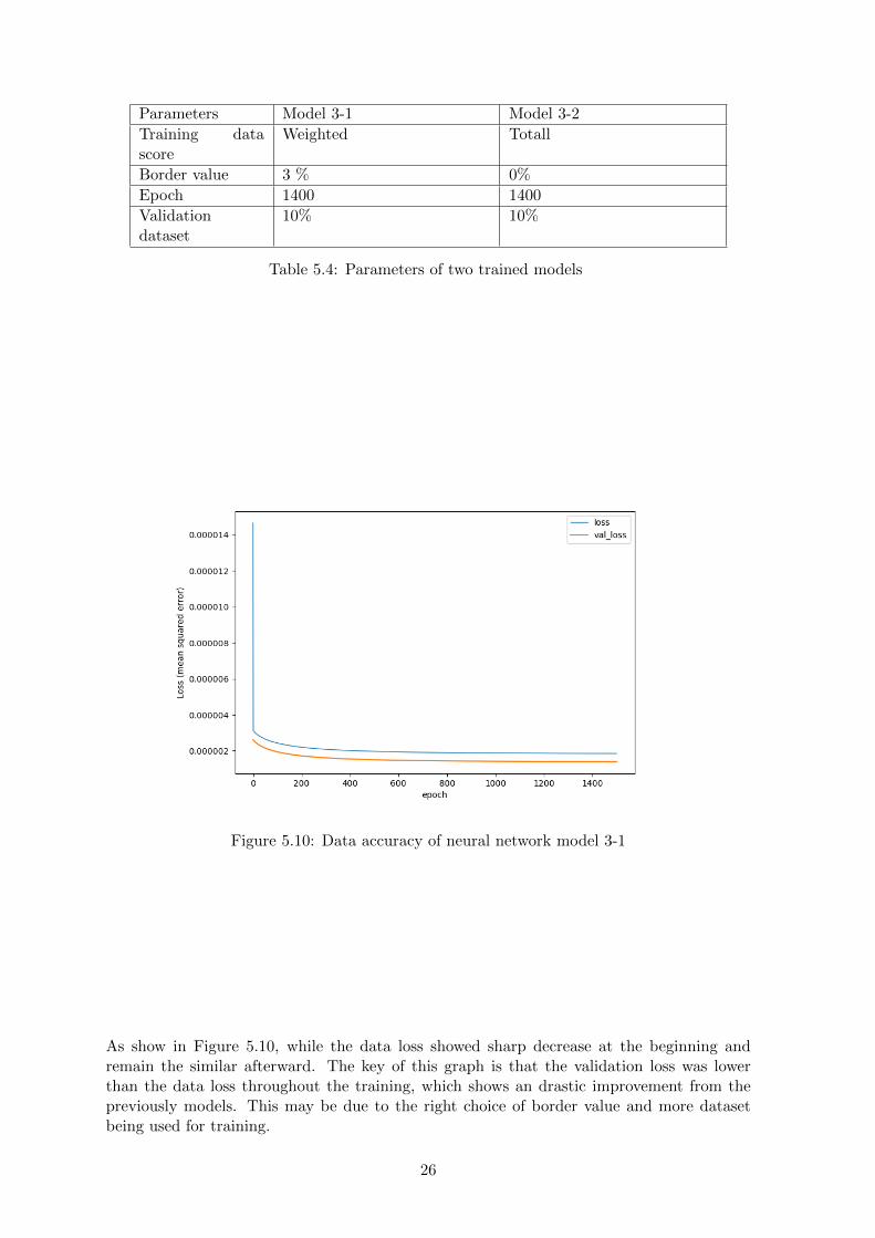
Parameters Model 3-1 Model 3-2
Training datascore
Weighted Totall
Border value 3 % 0%
Epoch 1400 1400
Validationdataset
10% 10%
Table 5.4: Parameters of two trained models
Figure 5.10: Data accuracy of neural network model 3-1
As show in Figure 5.10, while the data loss showed sharp decrease at the beginning andremain the similar afterward. The key of this graph is that the validation loss was lowerthan the data loss throughout the training, which shows an drastic improvement from thepreviously models. This may be due to the right choice of border value and more datasetbeing used for training.
26

Figure 5.11: Data accuracy of neural network model 3-2
Similar to Figure 5.10, Figure 5.11 also shows that the validation data loss and the data lossbeing quite close throughout the neural network training. However, a lot of spikes were foundand overall, both the validation data loss and the data loss fluctuated a lot, which indicatedthat the network model was not good as the previous Model 3.1.
While the overfitting problem seems to be solved, to improve the performance of the model,larger model can be bulit and trained with more dataset.
5.3.3 Training Result and Analysis - Testing against a Computer Othello
The trained networks were used as the evaluation function of computer Othello we developedand tested against the application The Othello. The results were shown as below:
27

Figure 5.12: Test Result of neural network model 3-1
Figure 5.13: Test result of neural network model 3-2
Figure 5.12 shows that the computer Othello with model 3-1 as evaluation function had awinning rate of 60% when playing against a moderate opponent, which indicates the achieve-ment of one of the project objectives. It had a winning rate of 20% when playing againsta strong opponent. On the other hand, Figure 5.13 shows that the computer Othello withmodel 3-2 as evaluation function had a winning rate of 40% when playing against a moderateopponent and no winning chance playing against a strong opponent. This matches with thedata accuracy results as analyzed above
During the game play, the computer Othello we developed with Model 3 could occupy thecorner once in a while, which shows that it became more sensitive to the preferable moves.While it still made moves at the dangerous zone, it could capture the opponent’s mistake andturned into his advantage, hencing winning the game eventually. This shows the improvementof the computer Othello in the game play.
28

Chapter 6
Conclusion and Future Research
6.1 Conclusions
This project aims to develop a computer Othello of size 8x8, where its evaluation functionbeing constructed without any human logic involved. The machine learning technique tobe used to achieve this purpose is deep learning neural network. The targeted winningrate is 50% when playing against a moderate opponent, and 35% when playing against astrong opponent. This objective was partially achieved by Model 3-1, where 3 convolutionallayers, 3 pooling layers and a fully-connected layer were being implemented as the hiddenlayers. While the overall result was not as satisfactory as expected, the experience and resultsobtained from this project might be useful for future computer Othello development usingdeep learning neural network.
6.2 Future Research Directions
For future development, more training data should be collected for the trainig purpose. Itis estimated that to develop a strong computer Othello, a million sets data are required.Moreover, it is important to capture the border during the training, hence in the cell valueassignment, it is advised to use a larger value to indicate the border region.
To allow more feature to be captured, a larger neural network should be designed and im-plemented for training. Though, developer must ensure the data sufficiency.
Different optimizers and loss function can also be used for the training in the hope to achievebetter result.
29

List of References
[1] Lee said: ’if alphago wants a rematch, i’d like to face it again’. [On-line]. Available: http://www.independent.co.uk/life-style/gadgets-and-tech/news/lee-sedol-alphago-google-deepmind-go-rematch-a6945831.html
[2] D. Eppstein. Minimax and negamax search. Emerging Technology. [Accessed 15-Sep-2016]. [Online]. Available: https://www.ics.uci.edu/∼eppstein/180a/970417.html
[3] Deep learning machine teaches itself chess in 72 hours, playsat international master level. Emerging Technology. [Accessed 15-Sep-2016]. [Online]. Available: https://www.technologyreview.com/s/541276/deep-learning-machine-teaches-itself-chess-in-72-hours-plays-at-international-master/
[4] Chapter 11 book openings. Othello Sky. [Accessed 17-Sep-2016]. [Online]. Available:http://www.soongsky.com/en/strategy2/ch11.php
[5] D. Silver. Mastering the game of go with deep neural networks and tree. [Accessed 10-Oct-2016]. [Online]. Available: http://www.nature.com/nature/journal/v529/n7587/full/nature16961.html
[6] J. Cirasella and D. Kopec. (2006) The history of computer games. Publicationsand Research Graduate Center, CUNY Academic Works, City University of NewYork (CUNY). [Online]. Available: http://academicworks.cuny.edu/cgi/viewcontent.cgi?article=1181&context=gc pubs
[7] M. Buro. (2003) The evolution of strong othello programs. NEC Research Institute.[Accessed 12-Apr-2017]. [Online]. Available: https://skatgame.net/mburo/ps/compoth.pdf
[8] M. van der Ree and M. Wiering. (2013) Reinforcement learning in the game of othello:Learning against a fixed opponent and learning from self-play. [Accessed: 24-Mar-2017]. [Online]. Available: http://www.ai.rug.nl/∼mwiering/GROUP/ARTICLES/paper-othello.pdf
[9] K. A. Cherry. (2011) An intelligent othello player combining machine learningand game specific heuristics. [Accessed: 16-Mar-2017]. [Online]. Available: http://protohacks.net/Papers/Thesis.pdf
[10] F. Chollet. Keras: Deep learning library for theano and tensorflow. [Online]. Available:https://keras.io/
[11] Deep learning tutorial. LISA lab, University of Montreal. [Accessed: 03-Sep-2016].[Online]. Available: http://deeplearning.net/tutorial/deeplearning.pdf
30

[12] V. Kovalev, A. Kalinovsky, and S. Kovalev. (2016) Deep learn-ing with theano, torch, caffe, tensorflow, and deeplearning4j: Whichone is the best in speed and accuracy? [Online]. Available: https://www.researchgate.net/publication/302955130 Deep Learning with Theano TorchCaffe TensorFlow and Deeplearning4J Which One Is the Best in Speed and Accuracy
[13] A. Ng, J. Ngiam, C. Y. Foo, Y. Mai, C. Suen, A. Coates, A. Maas,A. Hannun, B. Huval, T. Wang, and S. Tandon. Unsupervised feature learningand deep learning. Standford University. [Accessed 09-Jan-2017]. [Online]. Available:http://ufldl.stanford.edu/tutorial/supervised/ConvolutionalNeuralNetwork/
[14] N. Srivastava, G. Hinton, A. Krizhevsky, I. Sutskever, and R. Salakhutdinov, “Dropout:A simple way to prevent neural networks from overfitting,” Journal of MachineLearning Research, vol. 15, pp. 1929–1958, 2014, [Accessed 09-Mar-2017]. [Online].Available: http://www.cs.toronto.edu/∼rsalakhu/papers/srivastava14a.pdf/
[15] S. J. Russell and P. Norvig, “Artificial intelligence.” Prentice Hall, 2009, pp. 185–190.
[16] L. Brown. (2015) Deep learning with gpus. [Accessed: 18-Sep-2016]. [Online]. Available:http://www.nvidia.com/content/events/geoInt2015/LBrown DL.pdf
31

Appendix A
The game of Othello
Othello is a strategy game played by two players in black and white discs. The standardboard size is 8x8. The game starts from the board configuration with the four centeredsquares occupied as follows:
32

Figure A.1: Initial board position of Othello
The black player makes a move first, and the white player follows. A legal move requiresplayers to place a disc on an empty square adjacent to his opponents disc. Opponents discssandwiched between the newly placed disc and another disc of the same color along a linein any direction (horizontal, vertical, or diagonal) are flipped to match with the color of thenewly made move. An example of a legal move is shown below:
Figure A.2: A legal move in the game Othello.
33

In Figure A.2, Black player makes a move at the empty space C6, flipping the disc at positionsB5 across the horizontal line, B6 across the diagonal line, and C4 and C5 across the verticalline.
The game continues until no legal moves are available. When the game terminates, the playerwho has more discs on the board is the winner. When both players have the same amountof discs on the board, they tie the game.
34