pllution and working effects
TRANSCRIPT

862019 Pllution and Working Effects
httpslidepdfcomreaderfullpllution-and-working-effects 136
NBER WORKING PAPER SERIES
THE IMPACT OF POLLUTION ON WORKER PRODUCTIVITY
Joshua S Graff Zivin
Matthew J Neidell
Working Paper 17004
httpwwwnberorgpapersw17004
NATIONAL BUREAU OF ECONOMIC RESEARCH1050 Massachusetts Avenue
Cambridge MA 02138
April 2011
We thank numerous individuals and seminar participants at RAND UC-Irvine Maryland Cornell
Tufts Michigan University of Washington University of British Columbia CUNY Graduate Center
Yale University Columbia UC-San Diego and the NBER Health Economics meeting for helpful
suggestions We are also particularly indebted to Udi Sosnik for helping to make this project possible
and Shlomo Pleban for assistance in collecting the data both of Orange Enterprises We are grateful
for funding from the National Institute of Environmental Health Sciences (1R21ES019670-01) the
Property and Environment Research Center and seed grants from the Institute for Social and Economic
Research and Policy and the Northern Manhattan NIEHS The views expressed herein are those of
the authors and do not necessarily reflect the views of the National Bureau of Economic Research
copy 2011 by Joshua S Graff Zivin and Matthew J Neidell All rights reserved Short sections of text
not to exceed two paragraphs may be quoted without explicit permission provided that full credit
including copy notice is given to the source
862019 Pllution and Working Effects
httpslidepdfcomreaderfullpllution-and-working-effects 236
The Impact of Pollution on Worker Productivity
Joshua S Graff Zivin and Matthew J Neidell
NBER Working Paper No 17004
April 2011
JEL No I1J3Q5
ABSTRACT
Environmental protection is typically cast as a tax on the labor market and the economy in general
Since a large body of evidence links pollution with poor health and health is an important part of
human capital efforts to reduce pollution could plausibly be viewed as an investment in human capital
and thus a tool for promoting economic growth While a handful of studies have documented the impacts
of pollution on labor supply this paper is the first to rigorously assess the less visible but likely more
pervasive impacts on worker productivity In particular we exploit a novel panel dataset of daily farm
worker output as recorded under piece rate contracts merged with data on environmental conditions
to relate the plausibly exogenous daily variations in ozone with worker productivity We find robust
evidence that ozone levels well below federal air quality standards have a significant impact on productivity
a 10 ppb decrease in ozone concentrations increases worker productivity by 42 percent
Joshua S Graff Zivin
University of California San Diego
9500 Gilman Drive MC 0519
La Jolla CA 92093-0519
and NBER
jgraffzivinucsdedu
Matthew J Neidell
Department of Health Policy and Management
Columbia University
600 W 168th Street 6th Floor
New York NY 10032
and NBER
mn2191columbiaedu
862019 Pllution and Working Effects
httpslidepdfcomreaderfullpllution-and-working-effects 336
1 Introduction
As one of the primary factors of production labor is an essential element in every
nationrsquos economy Investing in human capital is widely viewed as a key to sustaining increases
in labor productivity and economic growth While health is increasingly seen as an important
part of human capital environmental protection which typically promotes health has not been
viewed through this lens Indeed such interventions are typically cast as a tax on producers and
consumers and thus a drag on the labor market and the economy in general Given the large
body of evidence that causally links pollution with poor health outcomes (eg Chay and
Greenstone 2003 Currie and Neidell 2005 Dockery et al 1993 Pope et al 2002 Bell et al
2004) it seems plausible that efforts to reduce pollution could in fact also be viewed as an
investment in human capital and thus a tool for promoting rather than retarding economic
growth
The key to this assertion lies in the impacts of pollution on labor market outcomes
While a handful of studies have documented impacts of pollution on labor supply (Ostro 1983
Hausman et al 1984 Graff Zivin and Neidell 2010 Carson et al 2010 Hanna and Oliva
2011)2 their focus on the extensive margin where behavioral responses are non-marginal only
captures high-visibility labor market impacts Pollution is also likely to have productivity
impacts on the intensive margin even in cases where labor supply remains unaffected Since
worker productivity is more difficult to monitor than labor supply these more subtle impacts
may be pervasive throughout the workplace so that even small individual effects may translate
into large welfare losses when aggregated across the economy There is however no systematic
2 Numerous cost-of-illness studies that focus on hospital outcomes such as length of hospital stay also implicitlyfocus on labor supply impacts
2
862019 Pllution and Working Effects
httpslidepdfcomreaderfullpllution-and-working-effects 436
evidence to date on the direct impact of pollution on worker productivity 3 This paper is the first
to rigorously assess this environmental productivity effect
Estimation of this relationship is complicated for two reasons One although datasets
frequently measure output per worker these measures do not isolate worker productivity from
other inputs (ie capital and technology) so that obtaining clean measures of worker
productivity is a perennial challenge Two exposure to pollution levels is typically endogenous
Since pollution is capitalized into housing prices (Chay and Greenstone 2005) individuals may
sort into areas with better air quality depending in part on their income which is a function of
their productivity (Banzhaf and Walsh 2008) Furthermore even if ambient pollution is
exogenous individuals may respond to ambient levels by reducing time spent outside so that
their exposure to pollution is endogenous (Neidell 2009)
In this paper we use a unique panel dataset on the productivity of agricultural workers to
overcome these challenges in analyzing the impact of ozone pollution on productivity Our data
on daily worker productivity is derived from an electronic payroll system used by a large farm in
the Central Valley of California who pays their employees through piece rate contracts A
growing body of evidence suggests that piece rates reduce shirking and increase productivity
over hourly wages and relative incentive schemes particularly in agricultural settings (Paarsch
and Shearar 1999 2000 Lazear 2000 Shi 2010 Bandiera et al 2005 2010) Given the
incentives under these contracts our measures of productivity can be viewed as a reasonable
proxy for productive capacity under typical work conditions
We conduct our analysis at a daily level to exploit the plausibly exogenous daily
fluctuations in ambient ozone concentrations Although aggregate variation in environmental
3In a notable case study Crocker and Horst (1981) examined the impacts of environmental conditions on 17 citrusharvesters They found a small negative impact on productivity from rather substantial levels of pollution inSouthern California in the early 1970s
3
862019 Pllution and Working Effects
httpslidepdfcomreaderfullpllution-and-working-effects 536
conditions is largely driven by economic activity daily variation in ozone is likely to be
exogenous Ozone is not directly emitted but forms from complex interactions between nitrogen
oxides (NOx) and volatile organic chemicals (VOCs) both of which are directly emitted in the
presence of heat and sunlight Thus ozone levels vary in part because of variations in
temperature but also because of the highly nonlinear relationship with NOx and VOCs For
example the ratio of NOx to VOCs is almost as important as the level of each in affecting ozone
levels (Auffhammer and Kellogg 2011) so that small decreases in NOx can even lead to
increases in ozone concentrations which has become the leading explanation behind the ldquoozone
weekend effectrdquo (Blanchard and Tanenbaum 2003) Moreover regional transport of NOx from
distant urban locations such as Los Angeles and San Francisco has a tremendous impact on
ozone levels in the Central Valley (Sillman 1999) Given the limited local sources of ozone
precursors this suggests that the ozone formation process coupled with emissions from distant
urban activities are the driving forces behind the daily variation in environmental conditions
observed near this farm
Furthermore the labor supply of agricultural workers is highly inelastic in the short run
Workers arrive at the field in crews and return as crews thus spending the majority of their day
outside regardless of environmental conditions Moreover since we have measures of both the
decision to work and the number of hours worked we can test whether workers respond to
ozone and in fact we are able to rule out even small changes in avoidance behavior Thus
focusing on agricultural workers greatly limits the scope for avoidance behavior further ensuring
that exposure to pollution is exogenous in this setting and that we are detecting productivity
impacts on the intensive margin
4
862019 Pllution and Working Effects
httpslidepdfcomreaderfullpllution-and-working-effects 636
After merging this worker data with environmental conditions based on readings from air
quality and meteorology stations in the California air monitoring network we estimate
econometric models that relate mean ozone concentrations during the typical work day to
productivity We find that ozone levels well below federal air quality standards have a
significant impact on productivity a 10 ppb decrease in ozone concentrations increases worker
productivity by 42 percent These effects are robust to various specification checks such as
flexible controls for temperature inclusion of lagged ozone concentrations and the inclusion of
worker fixed effects
Although these workers are paid through piece rate contracts worker compensation is
subject to minimum wage rules which can alter the incentive for workers to supply costly effort
To account for potential concerns about shirking we artificially induce ldquobottom-codingrdquo on
productivity measures for observations where the minimum wage binds and estimate both
parametric and semi-parametric censored regression models Under this specification the actual
measures of productivity when the minimum wage binds no longer influence estimates of the
impact of ozone on productivity Thus if the marginal effects of productivity on this latent
variable differ from the marginal effects from our baseline linear model this would indicate
shirking is occurring Our results however remain unchanged suggesting that the threat of
termination provides sufficient incentives for workers to supply effort even when compensation
is not directly tied to output Consistent with this explanation we find that employee separations
are significantly correlated with low-levels of productivity
These impacts are particularly noteworthy as the US Environmental Protection Agency
is currently contemplating a reduction in the federal ground-level ozone standard of
approximately 10 ppb (EPA 2010) The environmental productivity effect estimated in this
5
862019 Pllution and Working Effects
httpslidepdfcomreaderfullpllution-and-working-effects 736
paper offers a novel measure of morbidity impacts that are both more subtle and more pervasive
than the standard health impact measures based on hospitalizations and physician visits
Moreover they have the advantage of already being monetized for use in the regulatory cost-
benefit calculations required by Executive Order 12866 In developing countries where
environmental regulations are typically less stringent and agriculture plays a more prominent role
in the economy this environmental productivity effect may have particularly detrimental impacts
on national prosperity
The paper is organized as follows Section 2 describes the piece rate and environmental
data Section 3 provides a conceptual framework that largely serves to guide our econometric
model which is described in Section 4 Section 5 describes the results with a conclusion
provided in Section 6
2 Data
Our data comes from a unique arrangement with an international software provider
Orange Enterprises (OE) OE customizes paperless payroll collection for clients called the
Payroll Employee Tracking (PET) Tiger software system It tracks the progress of employees by
collecting real-time data on attendance and harvest levels of individual farm workers in order to
facilitate employee and payroll management The PET Tiger software operates as follows The
software is installed on handheld computers used by field supervisors At the beginning of the
day supervisors enter the date starting time and the crop being harvested Each employee
clocks in by scanning the unique barcode on his or her badge Each time the employee brings a
bushel bucket lug or bin his or her badge is swiped recording the unit and time Data
6
862019 Pllution and Working Effects
httpslidepdfcomreaderfullpllution-and-working-effects 836
collected in the field is transmitted to a host computer by synchronizing the handheld with the
host computer which facilitates the calculation of worker wages
We have purchased the rights to data from a farm in the Central Valley of California that
uses this system To protect the identity of the farm we can only reveal limited information
about their operations The farm with a total size of roughly 500 acres produces blueberries and
two types of grapes during the warmer months of the year The farm offers two distinct piece
rate contracts depending on the crop being harvested time plus pieces (TPP) for the grapes and
time plus all pieces (TPAP) for blueberries Total daily wages (w) from each contract can be
described by the following equations
(1) TPP w = 8h + p(q-minpcsh) I(qgtminpcsh)
TPAP w = 8h + pq I(qgtminpcsh)
where the minimum wage is $8 per hour h is hours worked p is the piece rate q is daily output
minpcs is the minimum number of hourly pieces to reach the piece rate regime and I is an
indicator function equal to 1 if the worker exceeds the minimum daily harvest threshold to
qualify for piece rate wages and 0 otherwise In both settings if the workerrsquos average hourly
output does not exceed minpcs the worker earns minimum wage The marginal incentive for a
worker whose output places them in the minimum wage portion of the compensation schedule is
job security In TPP the marginal incentive in the piece rate regime is the piece rate TPAP
slightly differs from TPP in that it pays piece rate for all pieces when a worker exceeds the
minimum hourly rate (as opposed to paying piece rate only for the pieces above the minimum)
Hence the payoff at minpcs is non-linear and thus provides a stronger incentive to reach this
threshold under this contract The incentive beyond this kink remains linear as under TPP
7
862019 Pllution and Working Effects
httpslidepdfcomreaderfullpllution-and-working-effects 936
862019 Pllution and Working Effects
httpslidepdfcomreaderfullpllution-and-working-effects 1036
higher than measurement from personal monitors attached to individuals in urban settings
(OrsquoNeill et al 2003) this is less of a concern in the agricultural setting where ratios of personal
to fixed monitors have been found to be as high as 096 (Brauer and Brook 1995) Furthermore
even when the difference exists the within-person variation is highly correlated with the within-
monitor variation (OrsquoNeill et al 2003) As a crude test for spatial uniformity of ozone levels
we regress ozone levels from the closest monitor to the farm against the second closest monitor
which is roughly 15 miles away and obtain an R-squared of 0888 Thus despite its simplicity
we expect measurement error using our proposed technique for assigning ozone to the farm to be
quite small
Our data follows roughly 1600 workers intermittently over 155 days Table 1 shows
summary statistics for worker output environmental variables and a breakdown of the sample
size There are three main crops harvested by this farm9 Under the TPAP contracts (which are
used to harvest crop type 1) workers are far less likely to reach the piece rate regime with this
happening for only 24 of workers compared to 57 and 47 for the other two crops which
are paid under TPP Among those workers whose output exceeds the levels that correspond to
the $8 per hour minimum wage the average hourly wages are $820 $828 and $888 for each
of the three crops respectively We also see that variation in worker output is equally driven by
variation within as well as across workers
In terms of environmental variables the average ambient ozone level for the day is under
50 ppb with a standard deviation of 13 ppb and a maximum of 86 ppb Since this measure of
ozone is taken over the average work day from 6 am ndash 3 pm it corresponds closely with national
8 Comparable R-squared for temperature is 094 and for particulate matter less than 25 μgm3 another pollutant of much interest is only 027 hence we do not focus on this important pollutant9 The timing of the harvest determines when each crop is ready to be picked so workers can not choose the crop onany given day
9
862019 Pllution and Working Effects
httpslidepdfcomreaderfullpllution-and-working-effects 1136
ambient air quality standards (NAAQS) which are based on 8-hour ozone measures Current
NAAQS are set at 75 ppb suggesting that while ozone levels during work hours can lead to
exceedances of air quality standards most work days are not in violation of regulatory
standards10 Consistent with the area being prone to ozone formation mean temperature and
sunlight (as proxied by solar radiation) are high and precipitation is low
For a deeper look at productivity Figure 1 plots the distribution of average pieces
collected per hour by crop and overall with a line drawn at the rate that corresponds with the
level of productivity that separates the minimum wage from the piece rate regime (the regime
threshold) To combine productivity across crops we standardize average hourly productivity by
subtracting the minimum number of pieces per hour required to reach the piece rate regime and
dividing by the standard deviation of productivity for each crop so the value that separates
regimes is 0 We can inspect these distributions to assess prima facie evidence of shirking If
shirking occurs when the minimum wage binds then we would expect part of the distribution to
be shifted away from the area just left of the regime threshold and into the left tail These plots
however do not exhibit such patterns For the two crops paid TPP the distribution of
productivity follows a symmetric normal distribution quite closely For the crop paid TPAP we
do see evidence of mass displaced just before the regime threshold However this mass is not
moved to the left tail but is instead shifted towards the right of the threshold Consistent with the
strong incentives associated with just crossing the threshold under this payment scheme workers
who are just below the threshold appear to increase their effort The pattern in all figures is
consistent with the notion that shirking among those receiving a fixed wage is minimal while
sorting around the regime threshold for crop 1 is not trivial
10 Violation of NAAQS is based on the daily maximum 8-hour ozone Since our measure of ozone begins at 6am atime when ozone levels are quite low the daily maximum 8-hour ozone is likely to be higher than our measure
10
862019 Pllution and Working Effects
httpslidepdfcomreaderfullpllution-and-working-effects 1236
The significant variation in pieces collected in Figure 1 is also noteworthy as this is
critical for obtaining precise estimates of the impact of ozone Figures 2 and 3 further illustrate
this variation both within and across workers For Figure 2 we collapse the data to the worker
level by computing each workerrsquos mean daily productivity over time For Figure 3 we collapse
the data to the daily level by computing the mean output of all workers on each day This
significant variation suggests that both worker ability and environmental conditions appear to be
important drivers of worker productivity
To illustrate the relationship between ozone and temperature Figure 4 plots the
demeaned average hourly ozone and temperature by day for the 2010 ozone season with an
indicator for days on which harvesting occurs This Figure reveals considerable variation in both
variables over time Importantly while ozone and temperature are often correlated ndash
temperature is an input into the production of ozone ndash there is ample independent variation for
conducting our proposed empirical tests11
We also take several steps to control for temperature
flexibly to ensure that we are properly accounting for this relationship
3 Conceptual framework
In this section we develop a simple conceptual model to illustrate worker incentives
under a piece rate regime with a minimum wage guarantee We begin by assuming that the
output q for any given worker is a function of effort e and pollution levels Ω Workers are paid
piece rate p per unit output but only if their total daily wage is at least as large as the daily
minimum wage 12
In anticipation of our empirical model we let zero denote the threshold
11 The R-squared from a regression of ozone on temperature alone is 061 When we more flexibly control for temperature and also include additional environmental variables the R-squared increases to 07012 While minimum wage standards are typically fixed at an hourly rate the fixed length workday in our settingallows us to translate this into a daily rate
11
862019 Pllution and Working Effects
httpslidepdfcomreaderfullpllution-and-working-effects 1336
level of output at which workers graduate from the minimum wage regime Since employment
contracts are extremely short-lived we assume that the probability of job retention τ is an
increasing function of output levels q when qlt013
Denoting the costs of worker effort as c(e)
and the value associated with job retention as k we can characterize the workersrsquo maximization
problem above and below the threshold output level
For those workers whose output level qualifies them for the piece rate wage (qge 0) effort
will be chosen in order to maximize the following
(2) Max e ( ) )( eceq p minusΩsdot
For those workers whose output level places them under the minimum wage regime (qlt0) effort
will be chosen to maximize the following
(3) Max e ndash τ (q(eΩ ))k ndash c(e)
The first order conditions for each are
(2rsquo) 0=part
partminus
part
partsdot
e
c
e
q p
(3rsquo) 0=part
partminus
part
part
part
partminus
e
ck
e
q
q
τ
Under the piece rate regime workers will supply effort such that the marginal cost of that effort
is equal to additional compensation associated with that effort For those workers being paid
minimum wage the incentive to supply effort is driven entirely by concerns about job security14
Workers supply effort such that the marginal cost of that effort is equal to the increased
probability of job retention associated with that effort times the value of job retention
13 The assumption of perfect retention for those above the threshold is made for simplicity As long as the probability of job retention is higher for those workers whose harvest levels exceed the threshold the basic intuition behind the results that follow remain unchanged
14 This is conceptually quite similar to the model of efficiency wages and unemployment advanced in Shapiro andStiglitz (1984) where high wages and the threat of unemployment induce workers to supply costly effort
12
862019 Pllution and Working Effects
httpslidepdfcomreaderfullpllution-and-working-effects 1436
The threat of punishment for low levels of output is instrumental in inducing effort under
the minimum wage regime If workers are homogenous and firms set contracts optimally the
gains from job retention due to extra effort will be set equal to the piece rate wage ie
pk q
=part
partminus
τ
such that effort exertion will be identical across both segments of the wage contract
If firms are unable to design optimal contracts effort will differ across regimes Of particular
concern is the situation in which termination incentives are low-powered ie pk q
ltpart
partminus
τ
In
this case workers essentially have a limited liability contract and thus have incentives to shirk
under the minimum wage regime Moreover since the productivity impacts of pollution increase
the probability of workers falling under the minimum wage portion of the compensation scheme
pollution will also indirectly increase the incentive to shirk Accounting for these potentially
different responses to pollution across regimes is central to our econometric model
4 Econometric Model
The worker maximization problem characterized in the previous section suggests the
following econometric model
(4) E[q|Ω X] = P(qge 0|Ω X)E[q|Ω Xqge 0] + (1-P(qge 0|Ω X))E[q|Ω Xqlt0]
where P is the probability a worker has output high enough to place them in the piece rate
regime 1-P is the probability a workerrsquos output places them in the minimum wage regime and X
are other factors that affect productivity (described in more detail below) We are primarily
interested in the direct effect of pollution on productivity (the environmental productivity effect)
Since there is no incentive to shirk in the piece rate regime δq δΩ represents the environmental
13
862019 Pllution and Working Effects
httpslidepdfcomreaderfullpllution-and-working-effects 1536
productivity effect15 To the extent that there is an incentive to shirk in the minimum wage
regime δq δΩ will reflect not only the environmental productivity effect but also the indirect
effect due to the interaction of this pollution effect with shirking incentives
We use two approaches for estimating this equation First we estimate a linear model
using all worker-day observations regardless of output levels and thus the payment regime
obtained that day
(5) q = β olsΩ + θ
ols X + ε
ols
where β ols
is the sum of the direct impact and if it exists the indirect impact of pollution on
productivity If the piece rate contract is set optimally by imposing an appropriate termination
threat as described in the previous section there is no incentive to shirk and β ols
will only
capture the environmental productivity effect To the extent that contracts are not set optimally
and there is an incentive to shirk in the minimum wage regime β ols will instead provide an upper
bound of the estimate of the environmental productivity effect because it will also include the
indirect effect of pollution on productivity via shirking
As a second approach we estimate equation (4) by artificially ldquobottom-codingrdquo our data
and estimating censored regression models To do this we leave all observations in the piece
rate regime as is but assign a measure of productivity of 0 to all observations in the minimum
wage regime16 Thus our estimation strategy can be viewed as a Type I Tobit model of the
following form
(6) q = β cen
Ω + θ cen
X + εcen
q = q if qge 0
15 Although environmental conditions may affect workers they may also have a direct impact on crops While thereis considerable evidence to support that chronic exposure to ozone affects crop yield (eg see Manning 2003) thereis no evidence to support an effect from acute exposure16 Because of our standardization of productivity a value of 0 represents the value when workers switch from theminimum wage to piece rate regime
14
862019 Pllution and Working Effects
httpslidepdfcomreaderfullpllution-and-working-effects 1636
q = 0 if qlt0
where q is the latent measure of productivity Because we are interested in the impact of
pollution on actual productivity which can take on values less than zero the environmental
productivity effect is the marginal effect of pollution on the latent variable q which is simply
β cen
Importantly the actual values of productivity in the minimum wage regime will have no
impact on the likelihood function and hence on β cen That is if shirking occurs so that the
distribution of productivity in the minimum wage regime is shifted to the left these observations
will no longer influence estimates of β cen
because they have been censored Instead only the
observations in the piece rate regime will affect estimates of β
cen
Therefore even if workers are
shirking when paid minimum wage our estimates of β cen
will only capture the environmental
productivity effect
The estimates from these two models can in turn be compared to test for the existence of
shirking If workers shirk when the minimum wage binds then we expect β ols
gt β cen
If workers
do not shirk when the minimum wage binds then we expect β ols
= β cen
We include data from all crops in one regression by using the standardized measures of
productivity described in the data section so the coefficients can be interpreted as a standard
deviation change in productivity from a 1 ppb change in ozone To control for other time-
varying factors that may affect productivity the vector X includes a quadratic in temperature
humidity precipitation wind speed air pressure and solar radiation all measured as the mean
over the typical work-day X also includes a series of day-of-week indicators to capture possible
changes in productivity throughout the week indicator variables for the crop to account for the
mean shift in productivity from different contracts and year-month dummies to control for
trends in pollution and productivity within and across growing seasons All standard errors are
15
862019 Pllution and Working Effects
httpslidepdfcomreaderfullpllution-and-working-effects 1736
two-way clustered on the date because the same environmental conditions are assigned to all
workers on a given day and on the worker to account for serial correlation in worker
productivity
Two facts about how ozone affects health are relevant for the econometric model One
chamber studies which randomly expose a small number of healthy young adults to varying
levels of ozone find that exposure to ozone can affect lung functioning in as quickly as within 1-
2 hours with effects exacerbated by exercise and with continued duration of exposure (see eg
Gong et al 1986 Kulle et al 1985 McDonnell et al 1983) These findings have generally
been confirmed in the field using outdoor workers mail carriers in Taichung City Taiwan and
agricultural workers in Fraser Valley Canada show decrements in lung functioning on days with
higher ozone concentrations (Chan and Wu 2005 Brauer et al 1996) As such we expect the
impact of ozone on productivity to be contemporaneous particularly given the strenuous nature
of this work and duration of exposure Two recovery from ozone pollution is fairly rapid when
removed from exposure Nearly all lung functioning returns to baseline levels in healthy adults
within 24 hours of exposure with recovery taking longer for hyperresponsive adults with
underlying health conditions (Folinsbee and Horvath 1989 Folinsbee and Hazucha 2000)17
Since ozone levels fall considerably overnight as heat and sunlight decline we expect lagged
ozone to have minimal impacts on the productivity of our healthy worker population Given
these two features of the dose-response to ozone we focus our analysis on the contemporaneous
relationship between ozone and productivity Nonetheless we explore the impact of lagged
ozone concentrations in order to confirm that our workers are indeed healthy
17 Although lung functioning recovers after exposure long term damage to lung cells may still occur (Tepper et al1989)
16
862019 Pllution and Working Effects
httpslidepdfcomreaderfullpllution-and-working-effects 1836
5 Results
To test the hypothesis that labor supply is inelastic in the short-run we begin by focusing
on whether work schedules respond to changes in ozone levels We estimate linear regression
models for the decision to work and the number of hours worked (conditional on working) both
with and without worker fixed effects Shown in Table 2 the results in the first two columns
which focus on the decision to work do not support evidence of a labor supply response to
ozone18 The second two columns also reveal that the number of hours worked is not
significantly related to ozone levels Even at the lower 95 confidence interval a 1 ppb increase
in ozone is associated with a 003 drop in hours worked which is a roughly 15 minute decrease
in hours worked The insensitivity of these results to including worker fixed effects strengthens
our confidence in these findings Thus consistent with our contention that avoidance behavior is
not an issue in this setting farm workers do not appear to adjust their work schedules in response
to ozone levels
In Table 3 we present our main results Column (1) presents results from our linear
regression model The estimated coefficient suggests that a 1 ppb increase in ozone leads to a
statistically significant decrease in productivity of 012 of a standard deviation Based on the
distribution of ozone and productivity in our sample this estimate implies that a 10 ppb decrease
in ozone increases worker productivity by 42 percent If wage contracts are set optimally this is
an unbiased estimate of the effect of ozone pollution If contracts are not set optimally and
workers shirk when the minimum wage binds then this estimate will overstate the impact of
ozone In column (2) we show results from a Type I Tobit model where we artificially censor
18 Marginal effects from logit and probit models for the decision to work are virtually identical to the results fromthe linear probability model
17
862019 Pllution and Working Effects
httpslidepdfcomreaderfullpllution-and-working-effects 1936
observations when the minimum wage binds and find an identical 012 standard deviation effect
from a 1 ppb change in ozone
Since this Tobit model assumes normality and homoskedasticity we assess the sensitivity
of our results to these assumptions by estimating a censored median regression model also
displaying results from an uncensored median regression model as a reference point19
Shown in
column (3) the median regression estimate is quite comparable to the linear regression estimate
which is not surprising given the distribution of productivity shown in Figure 1 The censored
median regression results shown in column (4) are also quite similar to the estimates from the
parametric censored models lending support to the parametric assumptions The comparability
of the four estimates in this Table suggests that shirking due to the minimum wage is relatively
minimal in this setting Thus the basic linear regression specification appears to yield unbiased
estimates of the pollution productivity effect
Although the lack of shirking in the minimum wage regime may appear surprising as
discussed in the conceptual framework this can arise if the gains from job retention associated
with providing effort are sufficiently large This is particularly important in our setting where
output is easily verified and labor contracts are extremely short-lived In order to examine the
potential importance of these features we provide descriptive evidence on the relationship
between worker productivity and separations We define a separation as the last day we observe
a worker in the data Similar to Lazear (2000) Table 4 shows the rate of separation by decile of
daily productivity Immediately evident is that less productive workers are more likely to
experience separations 65 percent of workers whose productivity falls in the bottom decile on
any given day separate from the farm while only 25 percent in the top decile separate (this
difference is statistically significant) As the next column shows highly productive workers
19 We estimate a censored median model using the 3-step procedure developed by Chernozhukov and Hong (2002)
18
862019 Pllution and Working Effects
httpslidepdfcomreaderfullpllution-and-working-effects 2036
typically have more tenure so some of these differences in separations could be driven by
differences in tenure In column (3) we show separations by productivity after adjusting for the
impact of tenure on productivity and find quite similar results Although we can not identify the
reason for a separation these results are consistent with the idea that the threat of termination for
less productive workers is reasonably high in this setting
In Table 5 we explore the sensitivity of both our linear and Tobit estimates to various
additional assumptions Column (1) repeats the baseline results In column (2) we include
worker fixed effects Although this increases the explanatory power of our regressions
considerably the estimates for ozone are largely unchanged consistent with the notion that
workers are not selecting into employment on any given day based on ozone concentrations
Since ozone is formed in part because of temperature and sunlight it is essential that we
properly control for these variables While we already control for a quadratic in mean
temperature and solar radiation we explore the sensitivity of the ozone estimates by also
including daily minimum and maximum temperature and solar radiation (column 3) and by
controlling for all three temperature measures more flexibly by using a series of indicator
variables for every 5 degrees Fahrenheit instead of a quadratic (column 4) Our estimates for
ozone remain largely unaffected by these changes suggesting that although ozone and
temperature are highly correlated the quadratic in mean temperature in our main specification
adequately controls for temperature
Figure 1 provided some evidence that worker effort changes near the regime threshold
particularly for crop 1 where contracts are time plus all pieces If higher ozone levels reduce
productivity and hence make it more likely for workers to fall into the minimum wage regime
this offsetting increase in effort may bias our results down In the remaining two columns of
19
862019 Pllution and Working Effects
httpslidepdfcomreaderfullpllution-and-working-effects 2136
Table 5 we address this by excluding observations that are close to the regime threshold varying
our definition of ldquocloserdquo20 Consistent with expectations our results are slightly larger as we
exclude more observations but these differences are minimal
To address potential concerns about the cumulative effect of ozone exposure we also
present results that include 1 and 2-day lags of ozone Since ozone levels may only reflect
exposure on days when workers actually work we limit our focus to days when workers have
worked the previous day by excluding from our analysis the first one or two days of the
workweek depending on how many lags we include in our specification Table 6 column (1)
repeats our baseline results from the linear regression model Shown in column (2) are results
without any lags but excluding Monday which are slightly higher than the baseline results
Including 1 lag of ozone shown in column (3) we find that the coefficient on contemporaneous
ozone remains the same and lagged ozone is negative but statistically insignificant The results
in column (4) show that excluding the first two work days continues to increase the
contemporaneous coefficient on ozone Including two lags of ozone column (5) shows that the
coefficient on contemporaneous ozone remains statistically significant and again unchanged
while both lags of ozone are statistically insignificant Together these estimates suggest that the
predominant effect of ozone is from same day exposure with an overnight respite from ozone
sufficient for lung functioning to return to baseline levels Moreover this rapid recovery implies
that the environmental productivity effects measured in this paper are predominantly impacting a
healthy population21
20 We also estimated models that completely excluded observations under the time plus all pieces contract and our estimates for ozone were -010 for the linear model and -013 for the Tobit model which are largely the same asthose found when those observations were included21 Recall from Section 4 that chamber studies suggest a rapid recovery from ozone exposure for healthy individuals
20
862019 Pllution and Working Effects
httpslidepdfcomreaderfullpllution-and-working-effects 2236
6 Conclusion
In this paper we merge a unique dataset on individual-level daily harvest rates for
agricultural workers with data on environmental conditions to assess the impact of ozone
pollution on worker productivity We find that a 10 ppb change in average ozone exposure
results in a significant and robust 42 percent change in agricultural worker productivity Despite
the applicability of minimum wages and the incentive to shirk we find little evidence of
differential effects depending on whether or not the minimum wage binds Importantly this
environmental productivity effect suggests that common characterizations of environmental
protection as purely a tax on producers and consumers to be weighed against the consumption
benefits associated with improved environmental quality may be misguided Environmental
protection can also be viewed as an investment in human capital and its contribution to firm
productivity and economic growth should be incorporated in the calculus of policy makers
Our results also speak to the ongoing debates on ozone policy Ozone pollution
continues to be a pervasive environmental issue throughout much of the world Debates over the
optimal level of ozone have ensued for many years and current efforts to strengthen these
standards remain contentious Defining regulatory thresholds depends in part on the benefits
associated with avoided exposure which has traditionally been estimated through a focus on
high-visibility health effects such as hospitalizations The labor productivity impacts measured
in this paper help make these benefits calculations more complete Our results indicate that
ozone even at levels below current air quality standards in most of the world has significant
negative impacts on worker productivity suggesting that the strengthening of regulations on
ozone pollution would yield additional benefits
21
862019 Pllution and Working Effects
httpslidepdfcomreaderfullpllution-and-working-effects 2336
These impacts of ozone on agricultural workers are also important in their own right A
back-of-the envelope calculation that applies the environmental productivity effect estimated in
the Central Valley of California to the whole of the US suggests that a 10 ppb reduction in the
ozone standard would translate into an annual cost savings of approximately $11 billion in labor
expenditure22
In the developing world where national incomes depend more heavily on
agriculture these productivity effects are likely to have a much larger impact on the economy
These impacts may be especially large in countries like India China and Mexico where rapid
industrial growth and automobile penetration contribute precursor chemicals that contribute to
substantially higher levels of ozone pollution
While the impacts of ozone on agricultural productivity are large the generalizability of
these findings to other pollutants and industries is unclear Agricultural workers face
considerably higher levels of exposure to pollution than individuals who work indoors That
said roughly 118 percent of the US labor force works in an industry with regular exposure to
outdoor conditions and this figure is much higher for middle- and lower-income countries (Graff
Zivin and Neidell 2010) Moreover many forms of outdoor pollution diminish indoor air
quality as well For example indoor penetration of fine particulate matter ranges from 38-94
for typical residential homes in the US (Abt et al 2000) Examining the generalizability of the
environmental productivity effect estimated in this paper to other pollutants and industries
represents a fruitful area for future research
22 Total labor expenditure in US agriculture was approximately $265B in 2007 (USDA 2009)
22
862019 Pllution and Working Effects
httpslidepdfcomreaderfullpllution-and-working-effects 2436
References
Abt Eileen Helen H Suh Paul Catalano and Petros Koutrakis (2000) ldquoRelative Contributionof Outdoor and Indoor Particle Sources to Indoor Concentrationsrdquo Environmental Science and Technology 34 (17) pp 3579ndash3587
Auffhammer Maximilian and Ryan Kellogg (2011) ldquoClearing the Air The Effects of GasolineContent Regulation on Air Qualityrdquo American Economic Review forthcoming
Bandiera Oriana Iwan Barankay and Imran Rasul (2005) ldquoSocial Preferences and theResponse to Incentives Evidence from Personnel Datardquo Quarterly Journal of Economics
120(3) 917-962
Bandiera Oriana Iwan Barankay and Imran Rasul (2010) ldquoSocial Incentives in theWorkplacerdquo Review of Economic Studies 77(2) 417-458
Banzhaf H Spencer and Randall Walsh (2008) ldquoDo People Vote with Their Feet AnEmpirical Test of Tieboutrdquo American Economic Review 98(3) 843ndash63
Bell Michelle Aidan McDermott Scott Zeger Jonathan Samet Francesca Dominici (2004)ldquoOzone and Short-term Mortality in 95 US Urban Communities 1987-2000rdquo Journal of the American Medical Association 292 (19)
Blanchard Charles and Shelley Tanenbaum (2003) ldquoDifferences between Weekday andWeekend Air Pollutant Levels in Southern Californiardquo Journal of the Air and Waste
Management Association 53(7)
Brauer M and JR Brook (1995) ldquoPersonal and Fixed-Site Ozone Measurementswith a Passive Samplerrdquo Journal of the Air and Waste Management Association 45 (7) 529-537
Brauer M J Blair and S Vedal (1996) ldquoEffect of ambient ozone exposure on lung function infarm workersrdquo Am J Respir Crit Care Med 154(4) 981-987
Carson Richard Phoebe Koundouri and Ceacuteline Nauges (2010) ldquoArsenic Mitigation inBangladesh A Household Labor Market Approachrdquo American Journal of Agricultural Economics 92
Chan Chang-Chuan and Tsung-Huan Wu (2005) ldquoEffects of Ambient Ozone Exposure on MailCarriers Peak Expiratory Flow Ratesrdquo Environmental Health Perspectives 113(6) 735-738
Chay Kenneth and Michael Greenstone (2003) ldquoThe Impact of Air Pollution on InfantMortality Evidence from Geographic Variation in Pollution Shocks Induced by a RecessionrdquoQuarterly Journal of Economics 118(3) 1121-1167
23
862019 Pllution and Working Effects
httpslidepdfcomreaderfullpllution-and-working-effects 2536
Chay Kenneth and Michael Greenstone (2005) ldquoDoes Air Quality Matter Evidence from theHousing Marketrdquo Journal of Political Economy 113 376ndash424
Chernozhukov Victor and Han Hong (2002) ldquoThree-step censored quantile regression andextramarital affairsrdquo Journal of the American Statistical Association 97(459) 872-882
Currie Janet and Matthew Neidell (2005) ldquoAir Pollution and Infant Health What Can We Learnfrom Californias Recent Experiencerdquo Quarterly Journal of Economics 120(3) 1003-1030
Dockery Douglas W C Arden Pope Xiping Xu John D Spengler James H Ware Martha EFay Benjamin G Ferris and Frank E Speizer (1993) ldquoAn association between air pollution andmortality in six US citiesrdquo The New England Journal of Medicine 3291753-1759
Environmental Protection Agency (2010) ldquoNational Ambient Air Quality Standards for Ozone(Proposed Rule)rdquo Federal Register 7511 (January 19 2010) p 2938-3052
Folinsbee L J Hazucha M J (2000) ldquoTime course of response to ozone exposure in healthyadult femalesrdquo Inhalation Toxicol 12 151-167
Folinsbee L J Horvath S M (1986) ldquoPersistence of the acute effects of ozone exposurerdquo Aviat Space Environ Med 57 1136-1143
Gong H Jr Bradley P W Simmons M S Tashkin D P (1986) ldquoImpaired exercise performance and pulmonary function in elite cyclists during low-level ozone exposure in a hotenvironmentrdquo Am Rev Respir Dis 134 726-733
Graff Zivin Joshua and Matthew Neidell (2010) ldquoTemperature and the allocation of timeImplications for climate changerdquo NBER working paper 15717
Hanna Rema and Paulina Oliva (2011) ldquoThe Effect of Pollution on Labor Supply Evidencefrom a Natural Experiment in Mexico Cityrdquo Mimeo
Hazucha M J LJ Folinsbee and PA Bromberg (2003) ldquoDistribution and reproducibility of spirometric response to ozone by gender and agerdquo J Appl Physiol 95 1917-1925
Hausman Jerry Bart Ostro and David Wise (1984) ldquoAir Pollution and Lost Workrdquo NBER Working Paper No 1263
Kulle T J Sauder L R Hebel J R Chatham M D (1985) rdquoOzone response relationshipsin healthy nonsmokersrdquo Am Rev Respir Dis 132 36-41
Lazear Edward (2000) ldquoPerformance pay and productivityrdquo American Economic Review 90(5)1346-1361
24
862019 Pllution and Working Effects
httpslidepdfcomreaderfullpllution-and-working-effects 2636
Manning WJ (2003) ldquoAssessing plant responses to ambient ozone Growth of ozone-sensitiveloblolly pine seedlings treated with ethylenediurea (EDU) and sodium erythorbate (NaE)rdquo Environ Pollut 126(1) 73-81
McDonnell W F Horstman D H Hazucha M J Seal E Jr Haak E D Salaam S A
House D E (1983) ldquoPulmonary effects of ozone exposure during exercise dose-responsecharacteristicsrdquo J Appl Physiol Respir Environ Exercise Physiol 54 1345-1352
Neidell Matthew (2009) ldquoInformation Avoidance Behavior and Health The Effect of Ozoneon Asthma Hospitalizationsrdquo Journal of Human Resources 44(2)
ONeill MS Ramirez-Aguilar M Meneses-Gonzalez F Hernaacutendez-Avila M Geyh AS Sienra-Monge JJ Romieu I (2003) ldquoOzone exposure among Mexico City outdoor workersrdquo J Air
Waste Manag Assoc 53(3) 339-46
Ostro Bart (1983) ldquoThe Effects of Air Pollution on Work Lost and Morbidity Journal of
Environmental Economics and Management 10(4) 371-382
Paarsch Harry J and Bruce Shearer (1999) ldquoThe Response of Worker Effort to Piece RatesEvidence from the British Columbia Tree-Planting Industry Journal of Human Resources 34643-667
Paarsch Harry J and Bruce Shearer (2000) ldquoPiece Rates Fixed Wages and Incentive EffectsStatistical Evidence from Payroll Records International Economic Review 40 59-92
Pope CA III Burnett RT Thun MJ Calle EE Krewski D Ito K Thurston GD (2002) ldquoLungCancer Cardiopulmonary Mortality and Long-term Exposure to Fine Particulate Air Pollutionrdquo Journal of the American Medical Association 2871132-1141
Shapiro Carl and Joseph Stiglitz (1984) ldquoEquilibrium unemployment as a worker disciplinedevicerdquo American Economic Review 74(3)
Shi Lan (2010) ldquoIncentive Effect of Piece Rate Contracts Evidence from Two Small FieldExperimentsrdquo The BE Journal of Economic Analysis amp Policy 10(1) (Topics)
Sillman Sanford (1999) ldquoThe Relation Between Ozone NOx and Hydrocarbons in Urban andPolluted Rural Environmentsrdquo Atmospheric Environment 33 1821-1845
Tepper J S Costa D L Lehmann J R Weber M F Hatch G E (1989) ldquoUnattenuatedstructural and biochemical alterations in the rat lung during functional adaptation to ozonerdquo Am
Rev Respir Dis 140 493-501
USDA (2009) 2007 Census of Agriculture (AC-07-A-5) National Agricultural StatisticsService Washington DC
25
862019 Pllution and Working Effects
httpslidepdfcomreaderfullpllution-and-working-effects 2736
Figure 1 Standardized average hourly pieces collected by crop and for all crops
Notes We standardize average hourly productivity by subtracting the minimum number of pieces per hour requiredto reach the piece rate regime and dividing by the standard deviation of productivity for each crop The vertical linereflects the regime threshold for crossing from the minimum wage to the piece rate regime
0
2
4
6
0
2
4
6
-5 0 5 -5 0 5
Crop 1 (time+all pieces) Crop 2 (time+pieces $03p)
Crop 3 (time+pieces $1p) Total
D e n s i t y
26
862019 Pllution and Working Effects
httpslidepdfcomreaderfullpllution-and-working-effects 2836
Figure 2 Variation in productivity by worker all crops
0
1
2
3
4
5
D e n s i t y
-4 -2 0 2
27
862019 Pllution and Working Effects
httpslidepdfcomreaderfullpllution-and-working-effects 2936
Figure 3 Variation in productivity by day all crops
0
2
4
6
D e n s i t y
-3 -2 -1 0 1 2
28
862019 Pllution and Working Effects
httpslidepdfcomreaderfullpllution-and-working-effects 3036
Figure 4 Average demeaned daily ozone and temperature in 2010
-40
-30
-20
-10
0
10
20
30
40
50
512010 612010 712010 812010 912010 1012010
d e m e a n e d v a l u e
ozone temperature harves t day
29
862019 Pllution and Working Effects
httpslidepdfcomreaderfullpllution-and-working-effects 3136
Table 1 Summary statistics
A Productivity variables (n=36215)Observations mean SD SD within
worker SD between
workers
1 Minimum wage regimeHourly pieces (crop 1) 11753 203 057 044 047Hourly pieces (crop 2) 4114 308 077 065 069Hourly pieces (crop 3) 5920 229 048 031 044hours worked 21787 763 129 076 1202 Piece rate regimeHourly pieces (crop 1) 3675 342 040 030 032Hourly pieces (crop 2) 5512 492 085 061 064Hourly pieces (crop 3) 5241 388 082 050 066hours worked 14428 734 152 096 135
B Environmental variables (n=155)mean SD min maxozone (ppb) 4777 1324 1050 8600temperature (F) 7815 852 5630 9698atmospheric pressure (mb) 100155 648 98886 101259resultant wind speed (mph) 274 053 161 460solar radiation (Wm2) 83733 17407 18700 108333relative humidity () 4533 1004 2790 9350 precipitation (mm) 240 505 000 3548
C Sample
total of dates 155total of employees 1664mean of days with farm 20
Notes SD Standard deviation Crop 1 is time plus all pieces with a piece rate of $05piece and minimum pieces per hour of 3 Crop 2 is time plus pieces with a piece rate of $03piece and minimum pieces per hour of 4 Crop 3 istime plus pieces with a piece rate of $1piece and minimum pieces per hour of 3
30
862019 Pllution and Working Effects
httpslidepdfcomreaderfullpllution-and-working-effects 3236
Table 2 Regression results of the effect of ozone on avoidance behavior
1 2 3 4
extensive margin probability(work)
intensive margin hours worked
ozone (ppb) -00017 -00018 00014 00014[00020] [00021] [00123] [00125]worker fixed effect N Y N YObservations 39223 39223 36215 36215R-squared 011 016 024 027Standard errors clustered on date and worker in brackets significant at 10 significant at 5 significantat 1 All regressions include controls for temperature (quadratic) air pressure wind speed solar radiation relativehumidity precipitation day of week dummies monthyear dummies and piece rate contract type dummies Allenvironmental variables are the mean of hourly values from 6am-3pm
31
862019 Pllution and Working Effects
httpslidepdfcomreaderfullpllution-and-working-effects 3336
Table 3 Main regression results of the effect of ozone on productivity
1 2 3 4
ozone (ppb) -00116 -00123 -00092 -00124[00043] [00052] [00055] [00058]
model linear Tobit median censoredmedianObservations 36215 36215 36215 36215(Psuedo) R2 031 010 019 024Standard errors clustered on date and worker in brackets significant at 10 significant at 5 significantat 1 The dependent variable is standardized hourly pieces collected All regressions include controls for temperature (quadratic) air pressure wind speed solar radiation relative humidity precipitation day of week dummies monthyear dummies and piece rate contract type dummies All environmental variables are the mean of hourly values from 6am-3pm Bootstrapped standard errors for both median regressions were obtained using 50replications
32
862019 Pllution and Working Effects
httpslidepdfcomreaderfullpllution-and-working-effects 3436
Table 4 Separation rates by productivity decile
1 2 3 4
A Unadjusted productivity B Productivity adjusted for tenure
productivitydecile separation rate tenure (days) separation rate tenure (days)
1 0065 1244 0061 17992 0060 1555 0063 19203 0047 1658 0055 18474 0053 1896 0047 19475 0034 1864 0047 21566 0042 2128 0039 22137 0044 2109 0038 19248 0032 2227 0029 18729 0025 2324 0024 1941
10 0025 2431 0023 1817This table shows daily mean separation rates and tenure by productivity decile
33
862019 Pllution and Working Effects
httpslidepdfcomreaderfullpllution-and-working-effects 3536
Table 5 Sensitivity of regression results of the effect of ozone on productivity
1 2 3 4 5 6
A Linear model
ozone (ppb) -00116 -00097 -00125 -00111 -00129 -00136
[00043] [00041] [00045] [00050] [00048] [00052]R-squared 031 053 031 033 032 033
B Tobit model
ozone (ppb) -00123 -00105 -00121 -00130 -00146 -00154[00052] [00049] [00053] [00059] [00057] [00064]
Pseudo R-squared
010 031 010 011 012 013
model baseline worker fixed
effect
includemin and
max of temp(quadratic)and solar
rad
includemin and
max of temp(indicators)and solar
rad
excludeobs 1 SD
of regimethreshold
excludeobs 2 SD
of regimethreshold
Observations 36215 36215 36215 36215 32415 30239Standard errors clustered on date and worker in brackets significant at 10 significant at 5 significantat 1 The dependent variable is standardized hourly pieces collected All regressions include controls for temperature (quadratic except column 4 which includes indicator variables for every 5 degrees F) air pressurewind speed solar radiation relative humidity precipitation day of week dummies monthyear dummies and piecerate contract type dummies All environmental variables are based on hourly values from 6am-3pm
34
862019 Pllution and Working Effects
httpslidepdfcomreaderfullpllution-and-working-effects 3636
Table 6 Regression results of the effect of lagged ozone on productivity
1 2 3 4 5
A Linear model
ozone (ppb) -0011 -0013 -0013 -0016 -0015
[0004] [0005] [0005] [0005] [0005]1 lag ozone (ppb) -0004 -0006[0004] [0006]
2 lag ozone (ppb) 0003[0005]
R-squared 031 032 032 032 032
B Tobit model
ozone (ppb) -0012 -0013 -0012 -0016 -0014[0005] [0006] [0006] [0006] [0006]
1 lag ozone (ppb) -0003 -0003
[0005] [0007]2 lag ozone (ppb) 0001[0005]
Pseudo R-squared 010 010 010 010 010
Day(s) of week excluded
none Monday Monday Monday ampTuesday
Monday ampTuesday
Observations 35465 25456 25456 17498 17498Standard errors clustered on date and worker in brackets significant at 10 significant at 5 significantat 1 The dependent variable is standardized hourly pieces collected All regressions control for temperature(quadratic) air pressure wind speed solar radiation relative humidity precipitation day of week dummiesmonthyear dummies and piece rate contract type dummies All environmental variables are the mean of hourly
values from 6am-3pm

862019 Pllution and Working Effects
httpslidepdfcomreaderfullpllution-and-working-effects 936
862019 Pllution and Working Effects
httpslidepdfcomreaderfullpllution-and-working-effects 1036
higher than measurement from personal monitors attached to individuals in urban settings
(OrsquoNeill et al 2003) this is less of a concern in the agricultural setting where ratios of personal
to fixed monitors have been found to be as high as 096 (Brauer and Brook 1995) Furthermore
even when the difference exists the within-person variation is highly correlated with the within-
monitor variation (OrsquoNeill et al 2003) As a crude test for spatial uniformity of ozone levels
we regress ozone levels from the closest monitor to the farm against the second closest monitor
which is roughly 15 miles away and obtain an R-squared of 0888 Thus despite its simplicity
we expect measurement error using our proposed technique for assigning ozone to the farm to be
quite small
Our data follows roughly 1600 workers intermittently over 155 days Table 1 shows
summary statistics for worker output environmental variables and a breakdown of the sample
size There are three main crops harvested by this farm9 Under the TPAP contracts (which are
used to harvest crop type 1) workers are far less likely to reach the piece rate regime with this
happening for only 24 of workers compared to 57 and 47 for the other two crops which
are paid under TPP Among those workers whose output exceeds the levels that correspond to
the $8 per hour minimum wage the average hourly wages are $820 $828 and $888 for each
of the three crops respectively We also see that variation in worker output is equally driven by
variation within as well as across workers
In terms of environmental variables the average ambient ozone level for the day is under
50 ppb with a standard deviation of 13 ppb and a maximum of 86 ppb Since this measure of
ozone is taken over the average work day from 6 am ndash 3 pm it corresponds closely with national
8 Comparable R-squared for temperature is 094 and for particulate matter less than 25 μgm3 another pollutant of much interest is only 027 hence we do not focus on this important pollutant9 The timing of the harvest determines when each crop is ready to be picked so workers can not choose the crop onany given day
9
862019 Pllution and Working Effects
httpslidepdfcomreaderfullpllution-and-working-effects 1136
ambient air quality standards (NAAQS) which are based on 8-hour ozone measures Current
NAAQS are set at 75 ppb suggesting that while ozone levels during work hours can lead to
exceedances of air quality standards most work days are not in violation of regulatory
standards10 Consistent with the area being prone to ozone formation mean temperature and
sunlight (as proxied by solar radiation) are high and precipitation is low
For a deeper look at productivity Figure 1 plots the distribution of average pieces
collected per hour by crop and overall with a line drawn at the rate that corresponds with the
level of productivity that separates the minimum wage from the piece rate regime (the regime
threshold) To combine productivity across crops we standardize average hourly productivity by
subtracting the minimum number of pieces per hour required to reach the piece rate regime and
dividing by the standard deviation of productivity for each crop so the value that separates
regimes is 0 We can inspect these distributions to assess prima facie evidence of shirking If
shirking occurs when the minimum wage binds then we would expect part of the distribution to
be shifted away from the area just left of the regime threshold and into the left tail These plots
however do not exhibit such patterns For the two crops paid TPP the distribution of
productivity follows a symmetric normal distribution quite closely For the crop paid TPAP we
do see evidence of mass displaced just before the regime threshold However this mass is not
moved to the left tail but is instead shifted towards the right of the threshold Consistent with the
strong incentives associated with just crossing the threshold under this payment scheme workers
who are just below the threshold appear to increase their effort The pattern in all figures is
consistent with the notion that shirking among those receiving a fixed wage is minimal while
sorting around the regime threshold for crop 1 is not trivial
10 Violation of NAAQS is based on the daily maximum 8-hour ozone Since our measure of ozone begins at 6am atime when ozone levels are quite low the daily maximum 8-hour ozone is likely to be higher than our measure
10
862019 Pllution and Working Effects
httpslidepdfcomreaderfullpllution-and-working-effects 1236
The significant variation in pieces collected in Figure 1 is also noteworthy as this is
critical for obtaining precise estimates of the impact of ozone Figures 2 and 3 further illustrate
this variation both within and across workers For Figure 2 we collapse the data to the worker
level by computing each workerrsquos mean daily productivity over time For Figure 3 we collapse
the data to the daily level by computing the mean output of all workers on each day This
significant variation suggests that both worker ability and environmental conditions appear to be
important drivers of worker productivity
To illustrate the relationship between ozone and temperature Figure 4 plots the
demeaned average hourly ozone and temperature by day for the 2010 ozone season with an
indicator for days on which harvesting occurs This Figure reveals considerable variation in both
variables over time Importantly while ozone and temperature are often correlated ndash
temperature is an input into the production of ozone ndash there is ample independent variation for
conducting our proposed empirical tests11
We also take several steps to control for temperature
flexibly to ensure that we are properly accounting for this relationship
3 Conceptual framework
In this section we develop a simple conceptual model to illustrate worker incentives
under a piece rate regime with a minimum wage guarantee We begin by assuming that the
output q for any given worker is a function of effort e and pollution levels Ω Workers are paid
piece rate p per unit output but only if their total daily wage is at least as large as the daily
minimum wage 12
In anticipation of our empirical model we let zero denote the threshold
11 The R-squared from a regression of ozone on temperature alone is 061 When we more flexibly control for temperature and also include additional environmental variables the R-squared increases to 07012 While minimum wage standards are typically fixed at an hourly rate the fixed length workday in our settingallows us to translate this into a daily rate
11
862019 Pllution and Working Effects
httpslidepdfcomreaderfullpllution-and-working-effects 1336
level of output at which workers graduate from the minimum wage regime Since employment
contracts are extremely short-lived we assume that the probability of job retention τ is an
increasing function of output levels q when qlt013
Denoting the costs of worker effort as c(e)
and the value associated with job retention as k we can characterize the workersrsquo maximization
problem above and below the threshold output level
For those workers whose output level qualifies them for the piece rate wage (qge 0) effort
will be chosen in order to maximize the following
(2) Max e ( ) )( eceq p minusΩsdot
For those workers whose output level places them under the minimum wage regime (qlt0) effort
will be chosen to maximize the following
(3) Max e ndash τ (q(eΩ ))k ndash c(e)
The first order conditions for each are
(2rsquo) 0=part
partminus
part
partsdot
e
c
e
q p
(3rsquo) 0=part
partminus
part
part
part
partminus
e
ck
e
q
q
τ
Under the piece rate regime workers will supply effort such that the marginal cost of that effort
is equal to additional compensation associated with that effort For those workers being paid
minimum wage the incentive to supply effort is driven entirely by concerns about job security14
Workers supply effort such that the marginal cost of that effort is equal to the increased
probability of job retention associated with that effort times the value of job retention
13 The assumption of perfect retention for those above the threshold is made for simplicity As long as the probability of job retention is higher for those workers whose harvest levels exceed the threshold the basic intuition behind the results that follow remain unchanged
14 This is conceptually quite similar to the model of efficiency wages and unemployment advanced in Shapiro andStiglitz (1984) where high wages and the threat of unemployment induce workers to supply costly effort
12
862019 Pllution and Working Effects
httpslidepdfcomreaderfullpllution-and-working-effects 1436
The threat of punishment for low levels of output is instrumental in inducing effort under
the minimum wage regime If workers are homogenous and firms set contracts optimally the
gains from job retention due to extra effort will be set equal to the piece rate wage ie
pk q
=part
partminus
τ
such that effort exertion will be identical across both segments of the wage contract
If firms are unable to design optimal contracts effort will differ across regimes Of particular
concern is the situation in which termination incentives are low-powered ie pk q
ltpart
partminus
τ
In
this case workers essentially have a limited liability contract and thus have incentives to shirk
under the minimum wage regime Moreover since the productivity impacts of pollution increase
the probability of workers falling under the minimum wage portion of the compensation scheme
pollution will also indirectly increase the incentive to shirk Accounting for these potentially
different responses to pollution across regimes is central to our econometric model
4 Econometric Model
The worker maximization problem characterized in the previous section suggests the
following econometric model
(4) E[q|Ω X] = P(qge 0|Ω X)E[q|Ω Xqge 0] + (1-P(qge 0|Ω X))E[q|Ω Xqlt0]
where P is the probability a worker has output high enough to place them in the piece rate
regime 1-P is the probability a workerrsquos output places them in the minimum wage regime and X
are other factors that affect productivity (described in more detail below) We are primarily
interested in the direct effect of pollution on productivity (the environmental productivity effect)
Since there is no incentive to shirk in the piece rate regime δq δΩ represents the environmental
13
862019 Pllution and Working Effects
httpslidepdfcomreaderfullpllution-and-working-effects 1536
productivity effect15 To the extent that there is an incentive to shirk in the minimum wage
regime δq δΩ will reflect not only the environmental productivity effect but also the indirect
effect due to the interaction of this pollution effect with shirking incentives
We use two approaches for estimating this equation First we estimate a linear model
using all worker-day observations regardless of output levels and thus the payment regime
obtained that day
(5) q = β olsΩ + θ
ols X + ε
ols
where β ols
is the sum of the direct impact and if it exists the indirect impact of pollution on
productivity If the piece rate contract is set optimally by imposing an appropriate termination
threat as described in the previous section there is no incentive to shirk and β ols
will only
capture the environmental productivity effect To the extent that contracts are not set optimally
and there is an incentive to shirk in the minimum wage regime β ols will instead provide an upper
bound of the estimate of the environmental productivity effect because it will also include the
indirect effect of pollution on productivity via shirking
As a second approach we estimate equation (4) by artificially ldquobottom-codingrdquo our data
and estimating censored regression models To do this we leave all observations in the piece
rate regime as is but assign a measure of productivity of 0 to all observations in the minimum
wage regime16 Thus our estimation strategy can be viewed as a Type I Tobit model of the
following form
(6) q = β cen
Ω + θ cen
X + εcen
q = q if qge 0
15 Although environmental conditions may affect workers they may also have a direct impact on crops While thereis considerable evidence to support that chronic exposure to ozone affects crop yield (eg see Manning 2003) thereis no evidence to support an effect from acute exposure16 Because of our standardization of productivity a value of 0 represents the value when workers switch from theminimum wage to piece rate regime
14
862019 Pllution and Working Effects
httpslidepdfcomreaderfullpllution-and-working-effects 1636
q = 0 if qlt0
where q is the latent measure of productivity Because we are interested in the impact of
pollution on actual productivity which can take on values less than zero the environmental
productivity effect is the marginal effect of pollution on the latent variable q which is simply
β cen
Importantly the actual values of productivity in the minimum wage regime will have no
impact on the likelihood function and hence on β cen That is if shirking occurs so that the
distribution of productivity in the minimum wage regime is shifted to the left these observations
will no longer influence estimates of β cen
because they have been censored Instead only the
observations in the piece rate regime will affect estimates of β
cen
Therefore even if workers are
shirking when paid minimum wage our estimates of β cen
will only capture the environmental
productivity effect
The estimates from these two models can in turn be compared to test for the existence of
shirking If workers shirk when the minimum wage binds then we expect β ols
gt β cen
If workers
do not shirk when the minimum wage binds then we expect β ols
= β cen
We include data from all crops in one regression by using the standardized measures of
productivity described in the data section so the coefficients can be interpreted as a standard
deviation change in productivity from a 1 ppb change in ozone To control for other time-
varying factors that may affect productivity the vector X includes a quadratic in temperature
humidity precipitation wind speed air pressure and solar radiation all measured as the mean
over the typical work-day X also includes a series of day-of-week indicators to capture possible
changes in productivity throughout the week indicator variables for the crop to account for the
mean shift in productivity from different contracts and year-month dummies to control for
trends in pollution and productivity within and across growing seasons All standard errors are
15
862019 Pllution and Working Effects
httpslidepdfcomreaderfullpllution-and-working-effects 1736
two-way clustered on the date because the same environmental conditions are assigned to all
workers on a given day and on the worker to account for serial correlation in worker
productivity
Two facts about how ozone affects health are relevant for the econometric model One
chamber studies which randomly expose a small number of healthy young adults to varying
levels of ozone find that exposure to ozone can affect lung functioning in as quickly as within 1-
2 hours with effects exacerbated by exercise and with continued duration of exposure (see eg
Gong et al 1986 Kulle et al 1985 McDonnell et al 1983) These findings have generally
been confirmed in the field using outdoor workers mail carriers in Taichung City Taiwan and
agricultural workers in Fraser Valley Canada show decrements in lung functioning on days with
higher ozone concentrations (Chan and Wu 2005 Brauer et al 1996) As such we expect the
impact of ozone on productivity to be contemporaneous particularly given the strenuous nature
of this work and duration of exposure Two recovery from ozone pollution is fairly rapid when
removed from exposure Nearly all lung functioning returns to baseline levels in healthy adults
within 24 hours of exposure with recovery taking longer for hyperresponsive adults with
underlying health conditions (Folinsbee and Horvath 1989 Folinsbee and Hazucha 2000)17
Since ozone levels fall considerably overnight as heat and sunlight decline we expect lagged
ozone to have minimal impacts on the productivity of our healthy worker population Given
these two features of the dose-response to ozone we focus our analysis on the contemporaneous
relationship between ozone and productivity Nonetheless we explore the impact of lagged
ozone concentrations in order to confirm that our workers are indeed healthy
17 Although lung functioning recovers after exposure long term damage to lung cells may still occur (Tepper et al1989)
16
862019 Pllution and Working Effects
httpslidepdfcomreaderfullpllution-and-working-effects 1836
5 Results
To test the hypothesis that labor supply is inelastic in the short-run we begin by focusing
on whether work schedules respond to changes in ozone levels We estimate linear regression
models for the decision to work and the number of hours worked (conditional on working) both
with and without worker fixed effects Shown in Table 2 the results in the first two columns
which focus on the decision to work do not support evidence of a labor supply response to
ozone18 The second two columns also reveal that the number of hours worked is not
significantly related to ozone levels Even at the lower 95 confidence interval a 1 ppb increase
in ozone is associated with a 003 drop in hours worked which is a roughly 15 minute decrease
in hours worked The insensitivity of these results to including worker fixed effects strengthens
our confidence in these findings Thus consistent with our contention that avoidance behavior is
not an issue in this setting farm workers do not appear to adjust their work schedules in response
to ozone levels
In Table 3 we present our main results Column (1) presents results from our linear
regression model The estimated coefficient suggests that a 1 ppb increase in ozone leads to a
statistically significant decrease in productivity of 012 of a standard deviation Based on the
distribution of ozone and productivity in our sample this estimate implies that a 10 ppb decrease
in ozone increases worker productivity by 42 percent If wage contracts are set optimally this is
an unbiased estimate of the effect of ozone pollution If contracts are not set optimally and
workers shirk when the minimum wage binds then this estimate will overstate the impact of
ozone In column (2) we show results from a Type I Tobit model where we artificially censor
18 Marginal effects from logit and probit models for the decision to work are virtually identical to the results fromthe linear probability model
17
862019 Pllution and Working Effects
httpslidepdfcomreaderfullpllution-and-working-effects 1936
observations when the minimum wage binds and find an identical 012 standard deviation effect
from a 1 ppb change in ozone
Since this Tobit model assumes normality and homoskedasticity we assess the sensitivity
of our results to these assumptions by estimating a censored median regression model also
displaying results from an uncensored median regression model as a reference point19
Shown in
column (3) the median regression estimate is quite comparable to the linear regression estimate
which is not surprising given the distribution of productivity shown in Figure 1 The censored
median regression results shown in column (4) are also quite similar to the estimates from the
parametric censored models lending support to the parametric assumptions The comparability
of the four estimates in this Table suggests that shirking due to the minimum wage is relatively
minimal in this setting Thus the basic linear regression specification appears to yield unbiased
estimates of the pollution productivity effect
Although the lack of shirking in the minimum wage regime may appear surprising as
discussed in the conceptual framework this can arise if the gains from job retention associated
with providing effort are sufficiently large This is particularly important in our setting where
output is easily verified and labor contracts are extremely short-lived In order to examine the
potential importance of these features we provide descriptive evidence on the relationship
between worker productivity and separations We define a separation as the last day we observe
a worker in the data Similar to Lazear (2000) Table 4 shows the rate of separation by decile of
daily productivity Immediately evident is that less productive workers are more likely to
experience separations 65 percent of workers whose productivity falls in the bottom decile on
any given day separate from the farm while only 25 percent in the top decile separate (this
difference is statistically significant) As the next column shows highly productive workers
19 We estimate a censored median model using the 3-step procedure developed by Chernozhukov and Hong (2002)
18
862019 Pllution and Working Effects
httpslidepdfcomreaderfullpllution-and-working-effects 2036
typically have more tenure so some of these differences in separations could be driven by
differences in tenure In column (3) we show separations by productivity after adjusting for the
impact of tenure on productivity and find quite similar results Although we can not identify the
reason for a separation these results are consistent with the idea that the threat of termination for
less productive workers is reasonably high in this setting
In Table 5 we explore the sensitivity of both our linear and Tobit estimates to various
additional assumptions Column (1) repeats the baseline results In column (2) we include
worker fixed effects Although this increases the explanatory power of our regressions
considerably the estimates for ozone are largely unchanged consistent with the notion that
workers are not selecting into employment on any given day based on ozone concentrations
Since ozone is formed in part because of temperature and sunlight it is essential that we
properly control for these variables While we already control for a quadratic in mean
temperature and solar radiation we explore the sensitivity of the ozone estimates by also
including daily minimum and maximum temperature and solar radiation (column 3) and by
controlling for all three temperature measures more flexibly by using a series of indicator
variables for every 5 degrees Fahrenheit instead of a quadratic (column 4) Our estimates for
ozone remain largely unaffected by these changes suggesting that although ozone and
temperature are highly correlated the quadratic in mean temperature in our main specification
adequately controls for temperature
Figure 1 provided some evidence that worker effort changes near the regime threshold
particularly for crop 1 where contracts are time plus all pieces If higher ozone levels reduce
productivity and hence make it more likely for workers to fall into the minimum wage regime
this offsetting increase in effort may bias our results down In the remaining two columns of
19
862019 Pllution and Working Effects
httpslidepdfcomreaderfullpllution-and-working-effects 2136
Table 5 we address this by excluding observations that are close to the regime threshold varying
our definition of ldquocloserdquo20 Consistent with expectations our results are slightly larger as we
exclude more observations but these differences are minimal
To address potential concerns about the cumulative effect of ozone exposure we also
present results that include 1 and 2-day lags of ozone Since ozone levels may only reflect
exposure on days when workers actually work we limit our focus to days when workers have
worked the previous day by excluding from our analysis the first one or two days of the
workweek depending on how many lags we include in our specification Table 6 column (1)
repeats our baseline results from the linear regression model Shown in column (2) are results
without any lags but excluding Monday which are slightly higher than the baseline results
Including 1 lag of ozone shown in column (3) we find that the coefficient on contemporaneous
ozone remains the same and lagged ozone is negative but statistically insignificant The results
in column (4) show that excluding the first two work days continues to increase the
contemporaneous coefficient on ozone Including two lags of ozone column (5) shows that the
coefficient on contemporaneous ozone remains statistically significant and again unchanged
while both lags of ozone are statistically insignificant Together these estimates suggest that the
predominant effect of ozone is from same day exposure with an overnight respite from ozone
sufficient for lung functioning to return to baseline levels Moreover this rapid recovery implies
that the environmental productivity effects measured in this paper are predominantly impacting a
healthy population21
20 We also estimated models that completely excluded observations under the time plus all pieces contract and our estimates for ozone were -010 for the linear model and -013 for the Tobit model which are largely the same asthose found when those observations were included21 Recall from Section 4 that chamber studies suggest a rapid recovery from ozone exposure for healthy individuals
20
862019 Pllution and Working Effects
httpslidepdfcomreaderfullpllution-and-working-effects 2236
6 Conclusion
In this paper we merge a unique dataset on individual-level daily harvest rates for
agricultural workers with data on environmental conditions to assess the impact of ozone
pollution on worker productivity We find that a 10 ppb change in average ozone exposure
results in a significant and robust 42 percent change in agricultural worker productivity Despite
the applicability of minimum wages and the incentive to shirk we find little evidence of
differential effects depending on whether or not the minimum wage binds Importantly this
environmental productivity effect suggests that common characterizations of environmental
protection as purely a tax on producers and consumers to be weighed against the consumption
benefits associated with improved environmental quality may be misguided Environmental
protection can also be viewed as an investment in human capital and its contribution to firm
productivity and economic growth should be incorporated in the calculus of policy makers
Our results also speak to the ongoing debates on ozone policy Ozone pollution
continues to be a pervasive environmental issue throughout much of the world Debates over the
optimal level of ozone have ensued for many years and current efforts to strengthen these
standards remain contentious Defining regulatory thresholds depends in part on the benefits
associated with avoided exposure which has traditionally been estimated through a focus on
high-visibility health effects such as hospitalizations The labor productivity impacts measured
in this paper help make these benefits calculations more complete Our results indicate that
ozone even at levels below current air quality standards in most of the world has significant
negative impacts on worker productivity suggesting that the strengthening of regulations on
ozone pollution would yield additional benefits
21
862019 Pllution and Working Effects
httpslidepdfcomreaderfullpllution-and-working-effects 2336
These impacts of ozone on agricultural workers are also important in their own right A
back-of-the envelope calculation that applies the environmental productivity effect estimated in
the Central Valley of California to the whole of the US suggests that a 10 ppb reduction in the
ozone standard would translate into an annual cost savings of approximately $11 billion in labor
expenditure22
In the developing world where national incomes depend more heavily on
agriculture these productivity effects are likely to have a much larger impact on the economy
These impacts may be especially large in countries like India China and Mexico where rapid
industrial growth and automobile penetration contribute precursor chemicals that contribute to
substantially higher levels of ozone pollution
While the impacts of ozone on agricultural productivity are large the generalizability of
these findings to other pollutants and industries is unclear Agricultural workers face
considerably higher levels of exposure to pollution than individuals who work indoors That
said roughly 118 percent of the US labor force works in an industry with regular exposure to
outdoor conditions and this figure is much higher for middle- and lower-income countries (Graff
Zivin and Neidell 2010) Moreover many forms of outdoor pollution diminish indoor air
quality as well For example indoor penetration of fine particulate matter ranges from 38-94
for typical residential homes in the US (Abt et al 2000) Examining the generalizability of the
environmental productivity effect estimated in this paper to other pollutants and industries
represents a fruitful area for future research
22 Total labor expenditure in US agriculture was approximately $265B in 2007 (USDA 2009)
22
862019 Pllution and Working Effects
httpslidepdfcomreaderfullpllution-and-working-effects 2436
References
Abt Eileen Helen H Suh Paul Catalano and Petros Koutrakis (2000) ldquoRelative Contributionof Outdoor and Indoor Particle Sources to Indoor Concentrationsrdquo Environmental Science and Technology 34 (17) pp 3579ndash3587
Auffhammer Maximilian and Ryan Kellogg (2011) ldquoClearing the Air The Effects of GasolineContent Regulation on Air Qualityrdquo American Economic Review forthcoming
Bandiera Oriana Iwan Barankay and Imran Rasul (2005) ldquoSocial Preferences and theResponse to Incentives Evidence from Personnel Datardquo Quarterly Journal of Economics
120(3) 917-962
Bandiera Oriana Iwan Barankay and Imran Rasul (2010) ldquoSocial Incentives in theWorkplacerdquo Review of Economic Studies 77(2) 417-458
Banzhaf H Spencer and Randall Walsh (2008) ldquoDo People Vote with Their Feet AnEmpirical Test of Tieboutrdquo American Economic Review 98(3) 843ndash63
Bell Michelle Aidan McDermott Scott Zeger Jonathan Samet Francesca Dominici (2004)ldquoOzone and Short-term Mortality in 95 US Urban Communities 1987-2000rdquo Journal of the American Medical Association 292 (19)
Blanchard Charles and Shelley Tanenbaum (2003) ldquoDifferences between Weekday andWeekend Air Pollutant Levels in Southern Californiardquo Journal of the Air and Waste
Management Association 53(7)
Brauer M and JR Brook (1995) ldquoPersonal and Fixed-Site Ozone Measurementswith a Passive Samplerrdquo Journal of the Air and Waste Management Association 45 (7) 529-537
Brauer M J Blair and S Vedal (1996) ldquoEffect of ambient ozone exposure on lung function infarm workersrdquo Am J Respir Crit Care Med 154(4) 981-987
Carson Richard Phoebe Koundouri and Ceacuteline Nauges (2010) ldquoArsenic Mitigation inBangladesh A Household Labor Market Approachrdquo American Journal of Agricultural Economics 92
Chan Chang-Chuan and Tsung-Huan Wu (2005) ldquoEffects of Ambient Ozone Exposure on MailCarriers Peak Expiratory Flow Ratesrdquo Environmental Health Perspectives 113(6) 735-738
Chay Kenneth and Michael Greenstone (2003) ldquoThe Impact of Air Pollution on InfantMortality Evidence from Geographic Variation in Pollution Shocks Induced by a RecessionrdquoQuarterly Journal of Economics 118(3) 1121-1167
23
862019 Pllution and Working Effects
httpslidepdfcomreaderfullpllution-and-working-effects 2536
Chay Kenneth and Michael Greenstone (2005) ldquoDoes Air Quality Matter Evidence from theHousing Marketrdquo Journal of Political Economy 113 376ndash424
Chernozhukov Victor and Han Hong (2002) ldquoThree-step censored quantile regression andextramarital affairsrdquo Journal of the American Statistical Association 97(459) 872-882
Currie Janet and Matthew Neidell (2005) ldquoAir Pollution and Infant Health What Can We Learnfrom Californias Recent Experiencerdquo Quarterly Journal of Economics 120(3) 1003-1030
Dockery Douglas W C Arden Pope Xiping Xu John D Spengler James H Ware Martha EFay Benjamin G Ferris and Frank E Speizer (1993) ldquoAn association between air pollution andmortality in six US citiesrdquo The New England Journal of Medicine 3291753-1759
Environmental Protection Agency (2010) ldquoNational Ambient Air Quality Standards for Ozone(Proposed Rule)rdquo Federal Register 7511 (January 19 2010) p 2938-3052
Folinsbee L J Hazucha M J (2000) ldquoTime course of response to ozone exposure in healthyadult femalesrdquo Inhalation Toxicol 12 151-167
Folinsbee L J Horvath S M (1986) ldquoPersistence of the acute effects of ozone exposurerdquo Aviat Space Environ Med 57 1136-1143
Gong H Jr Bradley P W Simmons M S Tashkin D P (1986) ldquoImpaired exercise performance and pulmonary function in elite cyclists during low-level ozone exposure in a hotenvironmentrdquo Am Rev Respir Dis 134 726-733
Graff Zivin Joshua and Matthew Neidell (2010) ldquoTemperature and the allocation of timeImplications for climate changerdquo NBER working paper 15717
Hanna Rema and Paulina Oliva (2011) ldquoThe Effect of Pollution on Labor Supply Evidencefrom a Natural Experiment in Mexico Cityrdquo Mimeo
Hazucha M J LJ Folinsbee and PA Bromberg (2003) ldquoDistribution and reproducibility of spirometric response to ozone by gender and agerdquo J Appl Physiol 95 1917-1925
Hausman Jerry Bart Ostro and David Wise (1984) ldquoAir Pollution and Lost Workrdquo NBER Working Paper No 1263
Kulle T J Sauder L R Hebel J R Chatham M D (1985) rdquoOzone response relationshipsin healthy nonsmokersrdquo Am Rev Respir Dis 132 36-41
Lazear Edward (2000) ldquoPerformance pay and productivityrdquo American Economic Review 90(5)1346-1361
24
862019 Pllution and Working Effects
httpslidepdfcomreaderfullpllution-and-working-effects 2636
Manning WJ (2003) ldquoAssessing plant responses to ambient ozone Growth of ozone-sensitiveloblolly pine seedlings treated with ethylenediurea (EDU) and sodium erythorbate (NaE)rdquo Environ Pollut 126(1) 73-81
McDonnell W F Horstman D H Hazucha M J Seal E Jr Haak E D Salaam S A
House D E (1983) ldquoPulmonary effects of ozone exposure during exercise dose-responsecharacteristicsrdquo J Appl Physiol Respir Environ Exercise Physiol 54 1345-1352
Neidell Matthew (2009) ldquoInformation Avoidance Behavior and Health The Effect of Ozoneon Asthma Hospitalizationsrdquo Journal of Human Resources 44(2)
ONeill MS Ramirez-Aguilar M Meneses-Gonzalez F Hernaacutendez-Avila M Geyh AS Sienra-Monge JJ Romieu I (2003) ldquoOzone exposure among Mexico City outdoor workersrdquo J Air
Waste Manag Assoc 53(3) 339-46
Ostro Bart (1983) ldquoThe Effects of Air Pollution on Work Lost and Morbidity Journal of
Environmental Economics and Management 10(4) 371-382
Paarsch Harry J and Bruce Shearer (1999) ldquoThe Response of Worker Effort to Piece RatesEvidence from the British Columbia Tree-Planting Industry Journal of Human Resources 34643-667
Paarsch Harry J and Bruce Shearer (2000) ldquoPiece Rates Fixed Wages and Incentive EffectsStatistical Evidence from Payroll Records International Economic Review 40 59-92
Pope CA III Burnett RT Thun MJ Calle EE Krewski D Ito K Thurston GD (2002) ldquoLungCancer Cardiopulmonary Mortality and Long-term Exposure to Fine Particulate Air Pollutionrdquo Journal of the American Medical Association 2871132-1141
Shapiro Carl and Joseph Stiglitz (1984) ldquoEquilibrium unemployment as a worker disciplinedevicerdquo American Economic Review 74(3)
Shi Lan (2010) ldquoIncentive Effect of Piece Rate Contracts Evidence from Two Small FieldExperimentsrdquo The BE Journal of Economic Analysis amp Policy 10(1) (Topics)
Sillman Sanford (1999) ldquoThe Relation Between Ozone NOx and Hydrocarbons in Urban andPolluted Rural Environmentsrdquo Atmospheric Environment 33 1821-1845
Tepper J S Costa D L Lehmann J R Weber M F Hatch G E (1989) ldquoUnattenuatedstructural and biochemical alterations in the rat lung during functional adaptation to ozonerdquo Am
Rev Respir Dis 140 493-501
USDA (2009) 2007 Census of Agriculture (AC-07-A-5) National Agricultural StatisticsService Washington DC
25
862019 Pllution and Working Effects
httpslidepdfcomreaderfullpllution-and-working-effects 2736
Figure 1 Standardized average hourly pieces collected by crop and for all crops
Notes We standardize average hourly productivity by subtracting the minimum number of pieces per hour requiredto reach the piece rate regime and dividing by the standard deviation of productivity for each crop The vertical linereflects the regime threshold for crossing from the minimum wage to the piece rate regime
0
2
4
6
0
2
4
6
-5 0 5 -5 0 5
Crop 1 (time+all pieces) Crop 2 (time+pieces $03p)
Crop 3 (time+pieces $1p) Total
D e n s i t y
26
862019 Pllution and Working Effects
httpslidepdfcomreaderfullpllution-and-working-effects 2836
Figure 2 Variation in productivity by worker all crops
0
1
2
3
4
5
D e n s i t y
-4 -2 0 2
27
862019 Pllution and Working Effects
httpslidepdfcomreaderfullpllution-and-working-effects 2936
Figure 3 Variation in productivity by day all crops
0
2
4
6
D e n s i t y
-3 -2 -1 0 1 2
28
862019 Pllution and Working Effects
httpslidepdfcomreaderfullpllution-and-working-effects 3036
Figure 4 Average demeaned daily ozone and temperature in 2010
-40
-30
-20
-10
0
10
20
30
40
50
512010 612010 712010 812010 912010 1012010
d e m e a n e d v a l u e
ozone temperature harves t day
29
862019 Pllution and Working Effects
httpslidepdfcomreaderfullpllution-and-working-effects 3136
Table 1 Summary statistics
A Productivity variables (n=36215)Observations mean SD SD within
worker SD between
workers
1 Minimum wage regimeHourly pieces (crop 1) 11753 203 057 044 047Hourly pieces (crop 2) 4114 308 077 065 069Hourly pieces (crop 3) 5920 229 048 031 044hours worked 21787 763 129 076 1202 Piece rate regimeHourly pieces (crop 1) 3675 342 040 030 032Hourly pieces (crop 2) 5512 492 085 061 064Hourly pieces (crop 3) 5241 388 082 050 066hours worked 14428 734 152 096 135
B Environmental variables (n=155)mean SD min maxozone (ppb) 4777 1324 1050 8600temperature (F) 7815 852 5630 9698atmospheric pressure (mb) 100155 648 98886 101259resultant wind speed (mph) 274 053 161 460solar radiation (Wm2) 83733 17407 18700 108333relative humidity () 4533 1004 2790 9350 precipitation (mm) 240 505 000 3548
C Sample
total of dates 155total of employees 1664mean of days with farm 20
Notes SD Standard deviation Crop 1 is time plus all pieces with a piece rate of $05piece and minimum pieces per hour of 3 Crop 2 is time plus pieces with a piece rate of $03piece and minimum pieces per hour of 4 Crop 3 istime plus pieces with a piece rate of $1piece and minimum pieces per hour of 3
30
862019 Pllution and Working Effects
httpslidepdfcomreaderfullpllution-and-working-effects 3236
Table 2 Regression results of the effect of ozone on avoidance behavior
1 2 3 4
extensive margin probability(work)
intensive margin hours worked
ozone (ppb) -00017 -00018 00014 00014[00020] [00021] [00123] [00125]worker fixed effect N Y N YObservations 39223 39223 36215 36215R-squared 011 016 024 027Standard errors clustered on date and worker in brackets significant at 10 significant at 5 significantat 1 All regressions include controls for temperature (quadratic) air pressure wind speed solar radiation relativehumidity precipitation day of week dummies monthyear dummies and piece rate contract type dummies Allenvironmental variables are the mean of hourly values from 6am-3pm
31
862019 Pllution and Working Effects
httpslidepdfcomreaderfullpllution-and-working-effects 3336
Table 3 Main regression results of the effect of ozone on productivity
1 2 3 4
ozone (ppb) -00116 -00123 -00092 -00124[00043] [00052] [00055] [00058]
model linear Tobit median censoredmedianObservations 36215 36215 36215 36215(Psuedo) R2 031 010 019 024Standard errors clustered on date and worker in brackets significant at 10 significant at 5 significantat 1 The dependent variable is standardized hourly pieces collected All regressions include controls for temperature (quadratic) air pressure wind speed solar radiation relative humidity precipitation day of week dummies monthyear dummies and piece rate contract type dummies All environmental variables are the mean of hourly values from 6am-3pm Bootstrapped standard errors for both median regressions were obtained using 50replications
32
862019 Pllution and Working Effects
httpslidepdfcomreaderfullpllution-and-working-effects 3436
Table 4 Separation rates by productivity decile
1 2 3 4
A Unadjusted productivity B Productivity adjusted for tenure
productivitydecile separation rate tenure (days) separation rate tenure (days)
1 0065 1244 0061 17992 0060 1555 0063 19203 0047 1658 0055 18474 0053 1896 0047 19475 0034 1864 0047 21566 0042 2128 0039 22137 0044 2109 0038 19248 0032 2227 0029 18729 0025 2324 0024 1941
10 0025 2431 0023 1817This table shows daily mean separation rates and tenure by productivity decile
33
862019 Pllution and Working Effects
httpslidepdfcomreaderfullpllution-and-working-effects 3536
Table 5 Sensitivity of regression results of the effect of ozone on productivity
1 2 3 4 5 6
A Linear model
ozone (ppb) -00116 -00097 -00125 -00111 -00129 -00136
[00043] [00041] [00045] [00050] [00048] [00052]R-squared 031 053 031 033 032 033
B Tobit model
ozone (ppb) -00123 -00105 -00121 -00130 -00146 -00154[00052] [00049] [00053] [00059] [00057] [00064]
Pseudo R-squared
010 031 010 011 012 013
model baseline worker fixed
effect
includemin and
max of temp(quadratic)and solar
rad
includemin and
max of temp(indicators)and solar
rad
excludeobs 1 SD
of regimethreshold
excludeobs 2 SD
of regimethreshold
Observations 36215 36215 36215 36215 32415 30239Standard errors clustered on date and worker in brackets significant at 10 significant at 5 significantat 1 The dependent variable is standardized hourly pieces collected All regressions include controls for temperature (quadratic except column 4 which includes indicator variables for every 5 degrees F) air pressurewind speed solar radiation relative humidity precipitation day of week dummies monthyear dummies and piecerate contract type dummies All environmental variables are based on hourly values from 6am-3pm
34
862019 Pllution and Working Effects
httpslidepdfcomreaderfullpllution-and-working-effects 3636
Table 6 Regression results of the effect of lagged ozone on productivity
1 2 3 4 5
A Linear model
ozone (ppb) -0011 -0013 -0013 -0016 -0015
[0004] [0005] [0005] [0005] [0005]1 lag ozone (ppb) -0004 -0006[0004] [0006]
2 lag ozone (ppb) 0003[0005]
R-squared 031 032 032 032 032
B Tobit model
ozone (ppb) -0012 -0013 -0012 -0016 -0014[0005] [0006] [0006] [0006] [0006]
1 lag ozone (ppb) -0003 -0003
[0005] [0007]2 lag ozone (ppb) 0001[0005]
Pseudo R-squared 010 010 010 010 010
Day(s) of week excluded
none Monday Monday Monday ampTuesday
Monday ampTuesday
Observations 35465 25456 25456 17498 17498Standard errors clustered on date and worker in brackets significant at 10 significant at 5 significantat 1 The dependent variable is standardized hourly pieces collected All regressions control for temperature(quadratic) air pressure wind speed solar radiation relative humidity precipitation day of week dummiesmonthyear dummies and piece rate contract type dummies All environmental variables are the mean of hourly
values from 6am-3pm
862019 Pllution and Working Effects
httpslidepdfcomreaderfullpllution-and-working-effects 1036
higher than measurement from personal monitors attached to individuals in urban settings
(OrsquoNeill et al 2003) this is less of a concern in the agricultural setting where ratios of personal
to fixed monitors have been found to be as high as 096 (Brauer and Brook 1995) Furthermore
even when the difference exists the within-person variation is highly correlated with the within-
monitor variation (OrsquoNeill et al 2003) As a crude test for spatial uniformity of ozone levels
we regress ozone levels from the closest monitor to the farm against the second closest monitor
which is roughly 15 miles away and obtain an R-squared of 0888 Thus despite its simplicity
we expect measurement error using our proposed technique for assigning ozone to the farm to be
quite small
Our data follows roughly 1600 workers intermittently over 155 days Table 1 shows
summary statistics for worker output environmental variables and a breakdown of the sample
size There are three main crops harvested by this farm9 Under the TPAP contracts (which are
used to harvest crop type 1) workers are far less likely to reach the piece rate regime with this
happening for only 24 of workers compared to 57 and 47 for the other two crops which
are paid under TPP Among those workers whose output exceeds the levels that correspond to
the $8 per hour minimum wage the average hourly wages are $820 $828 and $888 for each
of the three crops respectively We also see that variation in worker output is equally driven by
variation within as well as across workers
In terms of environmental variables the average ambient ozone level for the day is under
50 ppb with a standard deviation of 13 ppb and a maximum of 86 ppb Since this measure of
ozone is taken over the average work day from 6 am ndash 3 pm it corresponds closely with national
8 Comparable R-squared for temperature is 094 and for particulate matter less than 25 μgm3 another pollutant of much interest is only 027 hence we do not focus on this important pollutant9 The timing of the harvest determines when each crop is ready to be picked so workers can not choose the crop onany given day
9
862019 Pllution and Working Effects
httpslidepdfcomreaderfullpllution-and-working-effects 1136
ambient air quality standards (NAAQS) which are based on 8-hour ozone measures Current
NAAQS are set at 75 ppb suggesting that while ozone levels during work hours can lead to
exceedances of air quality standards most work days are not in violation of regulatory
standards10 Consistent with the area being prone to ozone formation mean temperature and
sunlight (as proxied by solar radiation) are high and precipitation is low
For a deeper look at productivity Figure 1 plots the distribution of average pieces
collected per hour by crop and overall with a line drawn at the rate that corresponds with the
level of productivity that separates the minimum wage from the piece rate regime (the regime
threshold) To combine productivity across crops we standardize average hourly productivity by
subtracting the minimum number of pieces per hour required to reach the piece rate regime and
dividing by the standard deviation of productivity for each crop so the value that separates
regimes is 0 We can inspect these distributions to assess prima facie evidence of shirking If
shirking occurs when the minimum wage binds then we would expect part of the distribution to
be shifted away from the area just left of the regime threshold and into the left tail These plots
however do not exhibit such patterns For the two crops paid TPP the distribution of
productivity follows a symmetric normal distribution quite closely For the crop paid TPAP we
do see evidence of mass displaced just before the regime threshold However this mass is not
moved to the left tail but is instead shifted towards the right of the threshold Consistent with the
strong incentives associated with just crossing the threshold under this payment scheme workers
who are just below the threshold appear to increase their effort The pattern in all figures is
consistent with the notion that shirking among those receiving a fixed wage is minimal while
sorting around the regime threshold for crop 1 is not trivial
10 Violation of NAAQS is based on the daily maximum 8-hour ozone Since our measure of ozone begins at 6am atime when ozone levels are quite low the daily maximum 8-hour ozone is likely to be higher than our measure
10
862019 Pllution and Working Effects
httpslidepdfcomreaderfullpllution-and-working-effects 1236
The significant variation in pieces collected in Figure 1 is also noteworthy as this is
critical for obtaining precise estimates of the impact of ozone Figures 2 and 3 further illustrate
this variation both within and across workers For Figure 2 we collapse the data to the worker
level by computing each workerrsquos mean daily productivity over time For Figure 3 we collapse
the data to the daily level by computing the mean output of all workers on each day This
significant variation suggests that both worker ability and environmental conditions appear to be
important drivers of worker productivity
To illustrate the relationship between ozone and temperature Figure 4 plots the
demeaned average hourly ozone and temperature by day for the 2010 ozone season with an
indicator for days on which harvesting occurs This Figure reveals considerable variation in both
variables over time Importantly while ozone and temperature are often correlated ndash
temperature is an input into the production of ozone ndash there is ample independent variation for
conducting our proposed empirical tests11
We also take several steps to control for temperature
flexibly to ensure that we are properly accounting for this relationship
3 Conceptual framework
In this section we develop a simple conceptual model to illustrate worker incentives
under a piece rate regime with a minimum wage guarantee We begin by assuming that the
output q for any given worker is a function of effort e and pollution levels Ω Workers are paid
piece rate p per unit output but only if their total daily wage is at least as large as the daily
minimum wage 12
In anticipation of our empirical model we let zero denote the threshold
11 The R-squared from a regression of ozone on temperature alone is 061 When we more flexibly control for temperature and also include additional environmental variables the R-squared increases to 07012 While minimum wage standards are typically fixed at an hourly rate the fixed length workday in our settingallows us to translate this into a daily rate
11
862019 Pllution and Working Effects
httpslidepdfcomreaderfullpllution-and-working-effects 1336
level of output at which workers graduate from the minimum wage regime Since employment
contracts are extremely short-lived we assume that the probability of job retention τ is an
increasing function of output levels q when qlt013
Denoting the costs of worker effort as c(e)
and the value associated with job retention as k we can characterize the workersrsquo maximization
problem above and below the threshold output level
For those workers whose output level qualifies them for the piece rate wage (qge 0) effort
will be chosen in order to maximize the following
(2) Max e ( ) )( eceq p minusΩsdot
For those workers whose output level places them under the minimum wage regime (qlt0) effort
will be chosen to maximize the following
(3) Max e ndash τ (q(eΩ ))k ndash c(e)
The first order conditions for each are
(2rsquo) 0=part
partminus
part
partsdot
e
c
e
q p
(3rsquo) 0=part
partminus
part
part
part
partminus
e
ck
e
q
q
τ
Under the piece rate regime workers will supply effort such that the marginal cost of that effort
is equal to additional compensation associated with that effort For those workers being paid
minimum wage the incentive to supply effort is driven entirely by concerns about job security14
Workers supply effort such that the marginal cost of that effort is equal to the increased
probability of job retention associated with that effort times the value of job retention
13 The assumption of perfect retention for those above the threshold is made for simplicity As long as the probability of job retention is higher for those workers whose harvest levels exceed the threshold the basic intuition behind the results that follow remain unchanged
14 This is conceptually quite similar to the model of efficiency wages and unemployment advanced in Shapiro andStiglitz (1984) where high wages and the threat of unemployment induce workers to supply costly effort
12
862019 Pllution and Working Effects
httpslidepdfcomreaderfullpllution-and-working-effects 1436
The threat of punishment for low levels of output is instrumental in inducing effort under
the minimum wage regime If workers are homogenous and firms set contracts optimally the
gains from job retention due to extra effort will be set equal to the piece rate wage ie
pk q
=part
partminus
τ
such that effort exertion will be identical across both segments of the wage contract
If firms are unable to design optimal contracts effort will differ across regimes Of particular
concern is the situation in which termination incentives are low-powered ie pk q
ltpart
partminus
τ
In
this case workers essentially have a limited liability contract and thus have incentives to shirk
under the minimum wage regime Moreover since the productivity impacts of pollution increase
the probability of workers falling under the minimum wage portion of the compensation scheme
pollution will also indirectly increase the incentive to shirk Accounting for these potentially
different responses to pollution across regimes is central to our econometric model
4 Econometric Model
The worker maximization problem characterized in the previous section suggests the
following econometric model
(4) E[q|Ω X] = P(qge 0|Ω X)E[q|Ω Xqge 0] + (1-P(qge 0|Ω X))E[q|Ω Xqlt0]
where P is the probability a worker has output high enough to place them in the piece rate
regime 1-P is the probability a workerrsquos output places them in the minimum wage regime and X
are other factors that affect productivity (described in more detail below) We are primarily
interested in the direct effect of pollution on productivity (the environmental productivity effect)
Since there is no incentive to shirk in the piece rate regime δq δΩ represents the environmental
13
862019 Pllution and Working Effects
httpslidepdfcomreaderfullpllution-and-working-effects 1536
productivity effect15 To the extent that there is an incentive to shirk in the minimum wage
regime δq δΩ will reflect not only the environmental productivity effect but also the indirect
effect due to the interaction of this pollution effect with shirking incentives
We use two approaches for estimating this equation First we estimate a linear model
using all worker-day observations regardless of output levels and thus the payment regime
obtained that day
(5) q = β olsΩ + θ
ols X + ε
ols
where β ols
is the sum of the direct impact and if it exists the indirect impact of pollution on
productivity If the piece rate contract is set optimally by imposing an appropriate termination
threat as described in the previous section there is no incentive to shirk and β ols
will only
capture the environmental productivity effect To the extent that contracts are not set optimally
and there is an incentive to shirk in the minimum wage regime β ols will instead provide an upper
bound of the estimate of the environmental productivity effect because it will also include the
indirect effect of pollution on productivity via shirking
As a second approach we estimate equation (4) by artificially ldquobottom-codingrdquo our data
and estimating censored regression models To do this we leave all observations in the piece
rate regime as is but assign a measure of productivity of 0 to all observations in the minimum
wage regime16 Thus our estimation strategy can be viewed as a Type I Tobit model of the
following form
(6) q = β cen
Ω + θ cen
X + εcen
q = q if qge 0
15 Although environmental conditions may affect workers they may also have a direct impact on crops While thereis considerable evidence to support that chronic exposure to ozone affects crop yield (eg see Manning 2003) thereis no evidence to support an effect from acute exposure16 Because of our standardization of productivity a value of 0 represents the value when workers switch from theminimum wage to piece rate regime
14
862019 Pllution and Working Effects
httpslidepdfcomreaderfullpllution-and-working-effects 1636
q = 0 if qlt0
where q is the latent measure of productivity Because we are interested in the impact of
pollution on actual productivity which can take on values less than zero the environmental
productivity effect is the marginal effect of pollution on the latent variable q which is simply
β cen
Importantly the actual values of productivity in the minimum wage regime will have no
impact on the likelihood function and hence on β cen That is if shirking occurs so that the
distribution of productivity in the minimum wage regime is shifted to the left these observations
will no longer influence estimates of β cen
because they have been censored Instead only the
observations in the piece rate regime will affect estimates of β
cen
Therefore even if workers are
shirking when paid minimum wage our estimates of β cen
will only capture the environmental
productivity effect
The estimates from these two models can in turn be compared to test for the existence of
shirking If workers shirk when the minimum wage binds then we expect β ols
gt β cen
If workers
do not shirk when the minimum wage binds then we expect β ols
= β cen
We include data from all crops in one regression by using the standardized measures of
productivity described in the data section so the coefficients can be interpreted as a standard
deviation change in productivity from a 1 ppb change in ozone To control for other time-
varying factors that may affect productivity the vector X includes a quadratic in temperature
humidity precipitation wind speed air pressure and solar radiation all measured as the mean
over the typical work-day X also includes a series of day-of-week indicators to capture possible
changes in productivity throughout the week indicator variables for the crop to account for the
mean shift in productivity from different contracts and year-month dummies to control for
trends in pollution and productivity within and across growing seasons All standard errors are
15
862019 Pllution and Working Effects
httpslidepdfcomreaderfullpllution-and-working-effects 1736
two-way clustered on the date because the same environmental conditions are assigned to all
workers on a given day and on the worker to account for serial correlation in worker
productivity
Two facts about how ozone affects health are relevant for the econometric model One
chamber studies which randomly expose a small number of healthy young adults to varying
levels of ozone find that exposure to ozone can affect lung functioning in as quickly as within 1-
2 hours with effects exacerbated by exercise and with continued duration of exposure (see eg
Gong et al 1986 Kulle et al 1985 McDonnell et al 1983) These findings have generally
been confirmed in the field using outdoor workers mail carriers in Taichung City Taiwan and
agricultural workers in Fraser Valley Canada show decrements in lung functioning on days with
higher ozone concentrations (Chan and Wu 2005 Brauer et al 1996) As such we expect the
impact of ozone on productivity to be contemporaneous particularly given the strenuous nature
of this work and duration of exposure Two recovery from ozone pollution is fairly rapid when
removed from exposure Nearly all lung functioning returns to baseline levels in healthy adults
within 24 hours of exposure with recovery taking longer for hyperresponsive adults with
underlying health conditions (Folinsbee and Horvath 1989 Folinsbee and Hazucha 2000)17
Since ozone levels fall considerably overnight as heat and sunlight decline we expect lagged
ozone to have minimal impacts on the productivity of our healthy worker population Given
these two features of the dose-response to ozone we focus our analysis on the contemporaneous
relationship between ozone and productivity Nonetheless we explore the impact of lagged
ozone concentrations in order to confirm that our workers are indeed healthy
17 Although lung functioning recovers after exposure long term damage to lung cells may still occur (Tepper et al1989)
16
862019 Pllution and Working Effects
httpslidepdfcomreaderfullpllution-and-working-effects 1836
5 Results
To test the hypothesis that labor supply is inelastic in the short-run we begin by focusing
on whether work schedules respond to changes in ozone levels We estimate linear regression
models for the decision to work and the number of hours worked (conditional on working) both
with and without worker fixed effects Shown in Table 2 the results in the first two columns
which focus on the decision to work do not support evidence of a labor supply response to
ozone18 The second two columns also reveal that the number of hours worked is not
significantly related to ozone levels Even at the lower 95 confidence interval a 1 ppb increase
in ozone is associated with a 003 drop in hours worked which is a roughly 15 minute decrease
in hours worked The insensitivity of these results to including worker fixed effects strengthens
our confidence in these findings Thus consistent with our contention that avoidance behavior is
not an issue in this setting farm workers do not appear to adjust their work schedules in response
to ozone levels
In Table 3 we present our main results Column (1) presents results from our linear
regression model The estimated coefficient suggests that a 1 ppb increase in ozone leads to a
statistically significant decrease in productivity of 012 of a standard deviation Based on the
distribution of ozone and productivity in our sample this estimate implies that a 10 ppb decrease
in ozone increases worker productivity by 42 percent If wage contracts are set optimally this is
an unbiased estimate of the effect of ozone pollution If contracts are not set optimally and
workers shirk when the minimum wage binds then this estimate will overstate the impact of
ozone In column (2) we show results from a Type I Tobit model where we artificially censor
18 Marginal effects from logit and probit models for the decision to work are virtually identical to the results fromthe linear probability model
17
862019 Pllution and Working Effects
httpslidepdfcomreaderfullpllution-and-working-effects 1936
observations when the minimum wage binds and find an identical 012 standard deviation effect
from a 1 ppb change in ozone
Since this Tobit model assumes normality and homoskedasticity we assess the sensitivity
of our results to these assumptions by estimating a censored median regression model also
displaying results from an uncensored median regression model as a reference point19
Shown in
column (3) the median regression estimate is quite comparable to the linear regression estimate
which is not surprising given the distribution of productivity shown in Figure 1 The censored
median regression results shown in column (4) are also quite similar to the estimates from the
parametric censored models lending support to the parametric assumptions The comparability
of the four estimates in this Table suggests that shirking due to the minimum wage is relatively
minimal in this setting Thus the basic linear regression specification appears to yield unbiased
estimates of the pollution productivity effect
Although the lack of shirking in the minimum wage regime may appear surprising as
discussed in the conceptual framework this can arise if the gains from job retention associated
with providing effort are sufficiently large This is particularly important in our setting where
output is easily verified and labor contracts are extremely short-lived In order to examine the
potential importance of these features we provide descriptive evidence on the relationship
between worker productivity and separations We define a separation as the last day we observe
a worker in the data Similar to Lazear (2000) Table 4 shows the rate of separation by decile of
daily productivity Immediately evident is that less productive workers are more likely to
experience separations 65 percent of workers whose productivity falls in the bottom decile on
any given day separate from the farm while only 25 percent in the top decile separate (this
difference is statistically significant) As the next column shows highly productive workers
19 We estimate a censored median model using the 3-step procedure developed by Chernozhukov and Hong (2002)
18
862019 Pllution and Working Effects
httpslidepdfcomreaderfullpllution-and-working-effects 2036
typically have more tenure so some of these differences in separations could be driven by
differences in tenure In column (3) we show separations by productivity after adjusting for the
impact of tenure on productivity and find quite similar results Although we can not identify the
reason for a separation these results are consistent with the idea that the threat of termination for
less productive workers is reasonably high in this setting
In Table 5 we explore the sensitivity of both our linear and Tobit estimates to various
additional assumptions Column (1) repeats the baseline results In column (2) we include
worker fixed effects Although this increases the explanatory power of our regressions
considerably the estimates for ozone are largely unchanged consistent with the notion that
workers are not selecting into employment on any given day based on ozone concentrations
Since ozone is formed in part because of temperature and sunlight it is essential that we
properly control for these variables While we already control for a quadratic in mean
temperature and solar radiation we explore the sensitivity of the ozone estimates by also
including daily minimum and maximum temperature and solar radiation (column 3) and by
controlling for all three temperature measures more flexibly by using a series of indicator
variables for every 5 degrees Fahrenheit instead of a quadratic (column 4) Our estimates for
ozone remain largely unaffected by these changes suggesting that although ozone and
temperature are highly correlated the quadratic in mean temperature in our main specification
adequately controls for temperature
Figure 1 provided some evidence that worker effort changes near the regime threshold
particularly for crop 1 where contracts are time plus all pieces If higher ozone levels reduce
productivity and hence make it more likely for workers to fall into the minimum wage regime
this offsetting increase in effort may bias our results down In the remaining two columns of
19
862019 Pllution and Working Effects
httpslidepdfcomreaderfullpllution-and-working-effects 2136
Table 5 we address this by excluding observations that are close to the regime threshold varying
our definition of ldquocloserdquo20 Consistent with expectations our results are slightly larger as we
exclude more observations but these differences are minimal
To address potential concerns about the cumulative effect of ozone exposure we also
present results that include 1 and 2-day lags of ozone Since ozone levels may only reflect
exposure on days when workers actually work we limit our focus to days when workers have
worked the previous day by excluding from our analysis the first one or two days of the
workweek depending on how many lags we include in our specification Table 6 column (1)
repeats our baseline results from the linear regression model Shown in column (2) are results
without any lags but excluding Monday which are slightly higher than the baseline results
Including 1 lag of ozone shown in column (3) we find that the coefficient on contemporaneous
ozone remains the same and lagged ozone is negative but statistically insignificant The results
in column (4) show that excluding the first two work days continues to increase the
contemporaneous coefficient on ozone Including two lags of ozone column (5) shows that the
coefficient on contemporaneous ozone remains statistically significant and again unchanged
while both lags of ozone are statistically insignificant Together these estimates suggest that the
predominant effect of ozone is from same day exposure with an overnight respite from ozone
sufficient for lung functioning to return to baseline levels Moreover this rapid recovery implies
that the environmental productivity effects measured in this paper are predominantly impacting a
healthy population21
20 We also estimated models that completely excluded observations under the time plus all pieces contract and our estimates for ozone were -010 for the linear model and -013 for the Tobit model which are largely the same asthose found when those observations were included21 Recall from Section 4 that chamber studies suggest a rapid recovery from ozone exposure for healthy individuals
20
862019 Pllution and Working Effects
httpslidepdfcomreaderfullpllution-and-working-effects 2236
6 Conclusion
In this paper we merge a unique dataset on individual-level daily harvest rates for
agricultural workers with data on environmental conditions to assess the impact of ozone
pollution on worker productivity We find that a 10 ppb change in average ozone exposure
results in a significant and robust 42 percent change in agricultural worker productivity Despite
the applicability of minimum wages and the incentive to shirk we find little evidence of
differential effects depending on whether or not the minimum wage binds Importantly this
environmental productivity effect suggests that common characterizations of environmental
protection as purely a tax on producers and consumers to be weighed against the consumption
benefits associated with improved environmental quality may be misguided Environmental
protection can also be viewed as an investment in human capital and its contribution to firm
productivity and economic growth should be incorporated in the calculus of policy makers
Our results also speak to the ongoing debates on ozone policy Ozone pollution
continues to be a pervasive environmental issue throughout much of the world Debates over the
optimal level of ozone have ensued for many years and current efforts to strengthen these
standards remain contentious Defining regulatory thresholds depends in part on the benefits
associated with avoided exposure which has traditionally been estimated through a focus on
high-visibility health effects such as hospitalizations The labor productivity impacts measured
in this paper help make these benefits calculations more complete Our results indicate that
ozone even at levels below current air quality standards in most of the world has significant
negative impacts on worker productivity suggesting that the strengthening of regulations on
ozone pollution would yield additional benefits
21
862019 Pllution and Working Effects
httpslidepdfcomreaderfullpllution-and-working-effects 2336
These impacts of ozone on agricultural workers are also important in their own right A
back-of-the envelope calculation that applies the environmental productivity effect estimated in
the Central Valley of California to the whole of the US suggests that a 10 ppb reduction in the
ozone standard would translate into an annual cost savings of approximately $11 billion in labor
expenditure22
In the developing world where national incomes depend more heavily on
agriculture these productivity effects are likely to have a much larger impact on the economy
These impacts may be especially large in countries like India China and Mexico where rapid
industrial growth and automobile penetration contribute precursor chemicals that contribute to
substantially higher levels of ozone pollution
While the impacts of ozone on agricultural productivity are large the generalizability of
these findings to other pollutants and industries is unclear Agricultural workers face
considerably higher levels of exposure to pollution than individuals who work indoors That
said roughly 118 percent of the US labor force works in an industry with regular exposure to
outdoor conditions and this figure is much higher for middle- and lower-income countries (Graff
Zivin and Neidell 2010) Moreover many forms of outdoor pollution diminish indoor air
quality as well For example indoor penetration of fine particulate matter ranges from 38-94
for typical residential homes in the US (Abt et al 2000) Examining the generalizability of the
environmental productivity effect estimated in this paper to other pollutants and industries
represents a fruitful area for future research
22 Total labor expenditure in US agriculture was approximately $265B in 2007 (USDA 2009)
22
862019 Pllution and Working Effects
httpslidepdfcomreaderfullpllution-and-working-effects 2436
References
Abt Eileen Helen H Suh Paul Catalano and Petros Koutrakis (2000) ldquoRelative Contributionof Outdoor and Indoor Particle Sources to Indoor Concentrationsrdquo Environmental Science and Technology 34 (17) pp 3579ndash3587
Auffhammer Maximilian and Ryan Kellogg (2011) ldquoClearing the Air The Effects of GasolineContent Regulation on Air Qualityrdquo American Economic Review forthcoming
Bandiera Oriana Iwan Barankay and Imran Rasul (2005) ldquoSocial Preferences and theResponse to Incentives Evidence from Personnel Datardquo Quarterly Journal of Economics
120(3) 917-962
Bandiera Oriana Iwan Barankay and Imran Rasul (2010) ldquoSocial Incentives in theWorkplacerdquo Review of Economic Studies 77(2) 417-458
Banzhaf H Spencer and Randall Walsh (2008) ldquoDo People Vote with Their Feet AnEmpirical Test of Tieboutrdquo American Economic Review 98(3) 843ndash63
Bell Michelle Aidan McDermott Scott Zeger Jonathan Samet Francesca Dominici (2004)ldquoOzone and Short-term Mortality in 95 US Urban Communities 1987-2000rdquo Journal of the American Medical Association 292 (19)
Blanchard Charles and Shelley Tanenbaum (2003) ldquoDifferences between Weekday andWeekend Air Pollutant Levels in Southern Californiardquo Journal of the Air and Waste
Management Association 53(7)
Brauer M and JR Brook (1995) ldquoPersonal and Fixed-Site Ozone Measurementswith a Passive Samplerrdquo Journal of the Air and Waste Management Association 45 (7) 529-537
Brauer M J Blair and S Vedal (1996) ldquoEffect of ambient ozone exposure on lung function infarm workersrdquo Am J Respir Crit Care Med 154(4) 981-987
Carson Richard Phoebe Koundouri and Ceacuteline Nauges (2010) ldquoArsenic Mitigation inBangladesh A Household Labor Market Approachrdquo American Journal of Agricultural Economics 92
Chan Chang-Chuan and Tsung-Huan Wu (2005) ldquoEffects of Ambient Ozone Exposure on MailCarriers Peak Expiratory Flow Ratesrdquo Environmental Health Perspectives 113(6) 735-738
Chay Kenneth and Michael Greenstone (2003) ldquoThe Impact of Air Pollution on InfantMortality Evidence from Geographic Variation in Pollution Shocks Induced by a RecessionrdquoQuarterly Journal of Economics 118(3) 1121-1167
23
862019 Pllution and Working Effects
httpslidepdfcomreaderfullpllution-and-working-effects 2536
Chay Kenneth and Michael Greenstone (2005) ldquoDoes Air Quality Matter Evidence from theHousing Marketrdquo Journal of Political Economy 113 376ndash424
Chernozhukov Victor and Han Hong (2002) ldquoThree-step censored quantile regression andextramarital affairsrdquo Journal of the American Statistical Association 97(459) 872-882
Currie Janet and Matthew Neidell (2005) ldquoAir Pollution and Infant Health What Can We Learnfrom Californias Recent Experiencerdquo Quarterly Journal of Economics 120(3) 1003-1030
Dockery Douglas W C Arden Pope Xiping Xu John D Spengler James H Ware Martha EFay Benjamin G Ferris and Frank E Speizer (1993) ldquoAn association between air pollution andmortality in six US citiesrdquo The New England Journal of Medicine 3291753-1759
Environmental Protection Agency (2010) ldquoNational Ambient Air Quality Standards for Ozone(Proposed Rule)rdquo Federal Register 7511 (January 19 2010) p 2938-3052
Folinsbee L J Hazucha M J (2000) ldquoTime course of response to ozone exposure in healthyadult femalesrdquo Inhalation Toxicol 12 151-167
Folinsbee L J Horvath S M (1986) ldquoPersistence of the acute effects of ozone exposurerdquo Aviat Space Environ Med 57 1136-1143
Gong H Jr Bradley P W Simmons M S Tashkin D P (1986) ldquoImpaired exercise performance and pulmonary function in elite cyclists during low-level ozone exposure in a hotenvironmentrdquo Am Rev Respir Dis 134 726-733
Graff Zivin Joshua and Matthew Neidell (2010) ldquoTemperature and the allocation of timeImplications for climate changerdquo NBER working paper 15717
Hanna Rema and Paulina Oliva (2011) ldquoThe Effect of Pollution on Labor Supply Evidencefrom a Natural Experiment in Mexico Cityrdquo Mimeo
Hazucha M J LJ Folinsbee and PA Bromberg (2003) ldquoDistribution and reproducibility of spirometric response to ozone by gender and agerdquo J Appl Physiol 95 1917-1925
Hausman Jerry Bart Ostro and David Wise (1984) ldquoAir Pollution and Lost Workrdquo NBER Working Paper No 1263
Kulle T J Sauder L R Hebel J R Chatham M D (1985) rdquoOzone response relationshipsin healthy nonsmokersrdquo Am Rev Respir Dis 132 36-41
Lazear Edward (2000) ldquoPerformance pay and productivityrdquo American Economic Review 90(5)1346-1361
24
862019 Pllution and Working Effects
httpslidepdfcomreaderfullpllution-and-working-effects 2636
Manning WJ (2003) ldquoAssessing plant responses to ambient ozone Growth of ozone-sensitiveloblolly pine seedlings treated with ethylenediurea (EDU) and sodium erythorbate (NaE)rdquo Environ Pollut 126(1) 73-81
McDonnell W F Horstman D H Hazucha M J Seal E Jr Haak E D Salaam S A
House D E (1983) ldquoPulmonary effects of ozone exposure during exercise dose-responsecharacteristicsrdquo J Appl Physiol Respir Environ Exercise Physiol 54 1345-1352
Neidell Matthew (2009) ldquoInformation Avoidance Behavior and Health The Effect of Ozoneon Asthma Hospitalizationsrdquo Journal of Human Resources 44(2)
ONeill MS Ramirez-Aguilar M Meneses-Gonzalez F Hernaacutendez-Avila M Geyh AS Sienra-Monge JJ Romieu I (2003) ldquoOzone exposure among Mexico City outdoor workersrdquo J Air
Waste Manag Assoc 53(3) 339-46
Ostro Bart (1983) ldquoThe Effects of Air Pollution on Work Lost and Morbidity Journal of
Environmental Economics and Management 10(4) 371-382
Paarsch Harry J and Bruce Shearer (1999) ldquoThe Response of Worker Effort to Piece RatesEvidence from the British Columbia Tree-Planting Industry Journal of Human Resources 34643-667
Paarsch Harry J and Bruce Shearer (2000) ldquoPiece Rates Fixed Wages and Incentive EffectsStatistical Evidence from Payroll Records International Economic Review 40 59-92
Pope CA III Burnett RT Thun MJ Calle EE Krewski D Ito K Thurston GD (2002) ldquoLungCancer Cardiopulmonary Mortality and Long-term Exposure to Fine Particulate Air Pollutionrdquo Journal of the American Medical Association 2871132-1141
Shapiro Carl and Joseph Stiglitz (1984) ldquoEquilibrium unemployment as a worker disciplinedevicerdquo American Economic Review 74(3)
Shi Lan (2010) ldquoIncentive Effect of Piece Rate Contracts Evidence from Two Small FieldExperimentsrdquo The BE Journal of Economic Analysis amp Policy 10(1) (Topics)
Sillman Sanford (1999) ldquoThe Relation Between Ozone NOx and Hydrocarbons in Urban andPolluted Rural Environmentsrdquo Atmospheric Environment 33 1821-1845
Tepper J S Costa D L Lehmann J R Weber M F Hatch G E (1989) ldquoUnattenuatedstructural and biochemical alterations in the rat lung during functional adaptation to ozonerdquo Am
Rev Respir Dis 140 493-501
USDA (2009) 2007 Census of Agriculture (AC-07-A-5) National Agricultural StatisticsService Washington DC
25
862019 Pllution and Working Effects
httpslidepdfcomreaderfullpllution-and-working-effects 2736
Figure 1 Standardized average hourly pieces collected by crop and for all crops
Notes We standardize average hourly productivity by subtracting the minimum number of pieces per hour requiredto reach the piece rate regime and dividing by the standard deviation of productivity for each crop The vertical linereflects the regime threshold for crossing from the minimum wage to the piece rate regime
0
2
4
6
0
2
4
6
-5 0 5 -5 0 5
Crop 1 (time+all pieces) Crop 2 (time+pieces $03p)
Crop 3 (time+pieces $1p) Total
D e n s i t y
26
862019 Pllution and Working Effects
httpslidepdfcomreaderfullpllution-and-working-effects 2836
Figure 2 Variation in productivity by worker all crops
0
1
2
3
4
5
D e n s i t y
-4 -2 0 2
27
862019 Pllution and Working Effects
httpslidepdfcomreaderfullpllution-and-working-effects 2936
Figure 3 Variation in productivity by day all crops
0
2
4
6
D e n s i t y
-3 -2 -1 0 1 2
28
862019 Pllution and Working Effects
httpslidepdfcomreaderfullpllution-and-working-effects 3036
Figure 4 Average demeaned daily ozone and temperature in 2010
-40
-30
-20
-10
0
10
20
30
40
50
512010 612010 712010 812010 912010 1012010
d e m e a n e d v a l u e
ozone temperature harves t day
29
862019 Pllution and Working Effects
httpslidepdfcomreaderfullpllution-and-working-effects 3136
Table 1 Summary statistics
A Productivity variables (n=36215)Observations mean SD SD within
worker SD between
workers
1 Minimum wage regimeHourly pieces (crop 1) 11753 203 057 044 047Hourly pieces (crop 2) 4114 308 077 065 069Hourly pieces (crop 3) 5920 229 048 031 044hours worked 21787 763 129 076 1202 Piece rate regimeHourly pieces (crop 1) 3675 342 040 030 032Hourly pieces (crop 2) 5512 492 085 061 064Hourly pieces (crop 3) 5241 388 082 050 066hours worked 14428 734 152 096 135
B Environmental variables (n=155)mean SD min maxozone (ppb) 4777 1324 1050 8600temperature (F) 7815 852 5630 9698atmospheric pressure (mb) 100155 648 98886 101259resultant wind speed (mph) 274 053 161 460solar radiation (Wm2) 83733 17407 18700 108333relative humidity () 4533 1004 2790 9350 precipitation (mm) 240 505 000 3548
C Sample
total of dates 155total of employees 1664mean of days with farm 20
Notes SD Standard deviation Crop 1 is time plus all pieces with a piece rate of $05piece and minimum pieces per hour of 3 Crop 2 is time plus pieces with a piece rate of $03piece and minimum pieces per hour of 4 Crop 3 istime plus pieces with a piece rate of $1piece and minimum pieces per hour of 3
30
862019 Pllution and Working Effects
httpslidepdfcomreaderfullpllution-and-working-effects 3236
Table 2 Regression results of the effect of ozone on avoidance behavior
1 2 3 4
extensive margin probability(work)
intensive margin hours worked
ozone (ppb) -00017 -00018 00014 00014[00020] [00021] [00123] [00125]worker fixed effect N Y N YObservations 39223 39223 36215 36215R-squared 011 016 024 027Standard errors clustered on date and worker in brackets significant at 10 significant at 5 significantat 1 All regressions include controls for temperature (quadratic) air pressure wind speed solar radiation relativehumidity precipitation day of week dummies monthyear dummies and piece rate contract type dummies Allenvironmental variables are the mean of hourly values from 6am-3pm
31
862019 Pllution and Working Effects
httpslidepdfcomreaderfullpllution-and-working-effects 3336
Table 3 Main regression results of the effect of ozone on productivity
1 2 3 4
ozone (ppb) -00116 -00123 -00092 -00124[00043] [00052] [00055] [00058]
model linear Tobit median censoredmedianObservations 36215 36215 36215 36215(Psuedo) R2 031 010 019 024Standard errors clustered on date and worker in brackets significant at 10 significant at 5 significantat 1 The dependent variable is standardized hourly pieces collected All regressions include controls for temperature (quadratic) air pressure wind speed solar radiation relative humidity precipitation day of week dummies monthyear dummies and piece rate contract type dummies All environmental variables are the mean of hourly values from 6am-3pm Bootstrapped standard errors for both median regressions were obtained using 50replications
32
862019 Pllution and Working Effects
httpslidepdfcomreaderfullpllution-and-working-effects 3436
Table 4 Separation rates by productivity decile
1 2 3 4
A Unadjusted productivity B Productivity adjusted for tenure
productivitydecile separation rate tenure (days) separation rate tenure (days)
1 0065 1244 0061 17992 0060 1555 0063 19203 0047 1658 0055 18474 0053 1896 0047 19475 0034 1864 0047 21566 0042 2128 0039 22137 0044 2109 0038 19248 0032 2227 0029 18729 0025 2324 0024 1941
10 0025 2431 0023 1817This table shows daily mean separation rates and tenure by productivity decile
33
862019 Pllution and Working Effects
httpslidepdfcomreaderfullpllution-and-working-effects 3536
Table 5 Sensitivity of regression results of the effect of ozone on productivity
1 2 3 4 5 6
A Linear model
ozone (ppb) -00116 -00097 -00125 -00111 -00129 -00136
[00043] [00041] [00045] [00050] [00048] [00052]R-squared 031 053 031 033 032 033
B Tobit model
ozone (ppb) -00123 -00105 -00121 -00130 -00146 -00154[00052] [00049] [00053] [00059] [00057] [00064]
Pseudo R-squared
010 031 010 011 012 013
model baseline worker fixed
effect
includemin and
max of temp(quadratic)and solar
rad
includemin and
max of temp(indicators)and solar
rad
excludeobs 1 SD
of regimethreshold
excludeobs 2 SD
of regimethreshold
Observations 36215 36215 36215 36215 32415 30239Standard errors clustered on date and worker in brackets significant at 10 significant at 5 significantat 1 The dependent variable is standardized hourly pieces collected All regressions include controls for temperature (quadratic except column 4 which includes indicator variables for every 5 degrees F) air pressurewind speed solar radiation relative humidity precipitation day of week dummies monthyear dummies and piecerate contract type dummies All environmental variables are based on hourly values from 6am-3pm
34
862019 Pllution and Working Effects
httpslidepdfcomreaderfullpllution-and-working-effects 3636
Table 6 Regression results of the effect of lagged ozone on productivity
1 2 3 4 5
A Linear model
ozone (ppb) -0011 -0013 -0013 -0016 -0015
[0004] [0005] [0005] [0005] [0005]1 lag ozone (ppb) -0004 -0006[0004] [0006]
2 lag ozone (ppb) 0003[0005]
R-squared 031 032 032 032 032
B Tobit model
ozone (ppb) -0012 -0013 -0012 -0016 -0014[0005] [0006] [0006] [0006] [0006]
1 lag ozone (ppb) -0003 -0003
[0005] [0007]2 lag ozone (ppb) 0001[0005]
Pseudo R-squared 010 010 010 010 010
Day(s) of week excluded
none Monday Monday Monday ampTuesday
Monday ampTuesday
Observations 35465 25456 25456 17498 17498Standard errors clustered on date and worker in brackets significant at 10 significant at 5 significantat 1 The dependent variable is standardized hourly pieces collected All regressions control for temperature(quadratic) air pressure wind speed solar radiation relative humidity precipitation day of week dummiesmonthyear dummies and piece rate contract type dummies All environmental variables are the mean of hourly
values from 6am-3pm

862019 Pllution and Working Effects
httpslidepdfcomreaderfullpllution-and-working-effects 1236
The significant variation in pieces collected in Figure 1 is also noteworthy as this is
critical for obtaining precise estimates of the impact of ozone Figures 2 and 3 further illustrate
this variation both within and across workers For Figure 2 we collapse the data to the worker
level by computing each workerrsquos mean daily productivity over time For Figure 3 we collapse
the data to the daily level by computing the mean output of all workers on each day This
significant variation suggests that both worker ability and environmental conditions appear to be
important drivers of worker productivity
To illustrate the relationship between ozone and temperature Figure 4 plots the
demeaned average hourly ozone and temperature by day for the 2010 ozone season with an
indicator for days on which harvesting occurs This Figure reveals considerable variation in both
variables over time Importantly while ozone and temperature are often correlated ndash
temperature is an input into the production of ozone ndash there is ample independent variation for
conducting our proposed empirical tests11
We also take several steps to control for temperature
flexibly to ensure that we are properly accounting for this relationship
3 Conceptual framework
In this section we develop a simple conceptual model to illustrate worker incentives
under a piece rate regime with a minimum wage guarantee We begin by assuming that the
output q for any given worker is a function of effort e and pollution levels Ω Workers are paid
piece rate p per unit output but only if their total daily wage is at least as large as the daily
minimum wage 12
In anticipation of our empirical model we let zero denote the threshold
11 The R-squared from a regression of ozone on temperature alone is 061 When we more flexibly control for temperature and also include additional environmental variables the R-squared increases to 07012 While minimum wage standards are typically fixed at an hourly rate the fixed length workday in our settingallows us to translate this into a daily rate
11
862019 Pllution and Working Effects
httpslidepdfcomreaderfullpllution-and-working-effects 1336
level of output at which workers graduate from the minimum wage regime Since employment
contracts are extremely short-lived we assume that the probability of job retention τ is an
increasing function of output levels q when qlt013
Denoting the costs of worker effort as c(e)
and the value associated with job retention as k we can characterize the workersrsquo maximization
problem above and below the threshold output level
For those workers whose output level qualifies them for the piece rate wage (qge 0) effort
will be chosen in order to maximize the following
(2) Max e ( ) )( eceq p minusΩsdot
For those workers whose output level places them under the minimum wage regime (qlt0) effort
will be chosen to maximize the following
(3) Max e ndash τ (q(eΩ ))k ndash c(e)
The first order conditions for each are
(2rsquo) 0=part
partminus
part
partsdot
e
c
e
q p
(3rsquo) 0=part
partminus
part
part
part
partminus
e
ck
e
q
q
τ
Under the piece rate regime workers will supply effort such that the marginal cost of that effort
is equal to additional compensation associated with that effort For those workers being paid
minimum wage the incentive to supply effort is driven entirely by concerns about job security14
Workers supply effort such that the marginal cost of that effort is equal to the increased
probability of job retention associated with that effort times the value of job retention
13 The assumption of perfect retention for those above the threshold is made for simplicity As long as the probability of job retention is higher for those workers whose harvest levels exceed the threshold the basic intuition behind the results that follow remain unchanged
14 This is conceptually quite similar to the model of efficiency wages and unemployment advanced in Shapiro andStiglitz (1984) where high wages and the threat of unemployment induce workers to supply costly effort
12
862019 Pllution and Working Effects
httpslidepdfcomreaderfullpllution-and-working-effects 1436
The threat of punishment for low levels of output is instrumental in inducing effort under
the minimum wage regime If workers are homogenous and firms set contracts optimally the
gains from job retention due to extra effort will be set equal to the piece rate wage ie
pk q
=part
partminus
τ
such that effort exertion will be identical across both segments of the wage contract
If firms are unable to design optimal contracts effort will differ across regimes Of particular
concern is the situation in which termination incentives are low-powered ie pk q
ltpart
partminus
τ
In
this case workers essentially have a limited liability contract and thus have incentives to shirk
under the minimum wage regime Moreover since the productivity impacts of pollution increase
the probability of workers falling under the minimum wage portion of the compensation scheme
pollution will also indirectly increase the incentive to shirk Accounting for these potentially
different responses to pollution across regimes is central to our econometric model
4 Econometric Model
The worker maximization problem characterized in the previous section suggests the
following econometric model
(4) E[q|Ω X] = P(qge 0|Ω X)E[q|Ω Xqge 0] + (1-P(qge 0|Ω X))E[q|Ω Xqlt0]
where P is the probability a worker has output high enough to place them in the piece rate
regime 1-P is the probability a workerrsquos output places them in the minimum wage regime and X
are other factors that affect productivity (described in more detail below) We are primarily
interested in the direct effect of pollution on productivity (the environmental productivity effect)
Since there is no incentive to shirk in the piece rate regime δq δΩ represents the environmental
13
862019 Pllution and Working Effects
httpslidepdfcomreaderfullpllution-and-working-effects 1536
productivity effect15 To the extent that there is an incentive to shirk in the minimum wage
regime δq δΩ will reflect not only the environmental productivity effect but also the indirect
effect due to the interaction of this pollution effect with shirking incentives
We use two approaches for estimating this equation First we estimate a linear model
using all worker-day observations regardless of output levels and thus the payment regime
obtained that day
(5) q = β olsΩ + θ
ols X + ε
ols
where β ols
is the sum of the direct impact and if it exists the indirect impact of pollution on
productivity If the piece rate contract is set optimally by imposing an appropriate termination
threat as described in the previous section there is no incentive to shirk and β ols
will only
capture the environmental productivity effect To the extent that contracts are not set optimally
and there is an incentive to shirk in the minimum wage regime β ols will instead provide an upper
bound of the estimate of the environmental productivity effect because it will also include the
indirect effect of pollution on productivity via shirking
As a second approach we estimate equation (4) by artificially ldquobottom-codingrdquo our data
and estimating censored regression models To do this we leave all observations in the piece
rate regime as is but assign a measure of productivity of 0 to all observations in the minimum
wage regime16 Thus our estimation strategy can be viewed as a Type I Tobit model of the
following form
(6) q = β cen
Ω + θ cen
X + εcen
q = q if qge 0
15 Although environmental conditions may affect workers they may also have a direct impact on crops While thereis considerable evidence to support that chronic exposure to ozone affects crop yield (eg see Manning 2003) thereis no evidence to support an effect from acute exposure16 Because of our standardization of productivity a value of 0 represents the value when workers switch from theminimum wage to piece rate regime
14
862019 Pllution and Working Effects
httpslidepdfcomreaderfullpllution-and-working-effects 1636
q = 0 if qlt0
where q is the latent measure of productivity Because we are interested in the impact of
pollution on actual productivity which can take on values less than zero the environmental
productivity effect is the marginal effect of pollution on the latent variable q which is simply
β cen
Importantly the actual values of productivity in the minimum wage regime will have no
impact on the likelihood function and hence on β cen That is if shirking occurs so that the
distribution of productivity in the minimum wage regime is shifted to the left these observations
will no longer influence estimates of β cen
because they have been censored Instead only the
observations in the piece rate regime will affect estimates of β
cen
Therefore even if workers are
shirking when paid minimum wage our estimates of β cen
will only capture the environmental
productivity effect
The estimates from these two models can in turn be compared to test for the existence of
shirking If workers shirk when the minimum wage binds then we expect β ols
gt β cen
If workers
do not shirk when the minimum wage binds then we expect β ols
= β cen
We include data from all crops in one regression by using the standardized measures of
productivity described in the data section so the coefficients can be interpreted as a standard
deviation change in productivity from a 1 ppb change in ozone To control for other time-
varying factors that may affect productivity the vector X includes a quadratic in temperature
humidity precipitation wind speed air pressure and solar radiation all measured as the mean
over the typical work-day X also includes a series of day-of-week indicators to capture possible
changes in productivity throughout the week indicator variables for the crop to account for the
mean shift in productivity from different contracts and year-month dummies to control for
trends in pollution and productivity within and across growing seasons All standard errors are
15
862019 Pllution and Working Effects
httpslidepdfcomreaderfullpllution-and-working-effects 1736
two-way clustered on the date because the same environmental conditions are assigned to all
workers on a given day and on the worker to account for serial correlation in worker
productivity
Two facts about how ozone affects health are relevant for the econometric model One
chamber studies which randomly expose a small number of healthy young adults to varying
levels of ozone find that exposure to ozone can affect lung functioning in as quickly as within 1-
2 hours with effects exacerbated by exercise and with continued duration of exposure (see eg
Gong et al 1986 Kulle et al 1985 McDonnell et al 1983) These findings have generally
been confirmed in the field using outdoor workers mail carriers in Taichung City Taiwan and
agricultural workers in Fraser Valley Canada show decrements in lung functioning on days with
higher ozone concentrations (Chan and Wu 2005 Brauer et al 1996) As such we expect the
impact of ozone on productivity to be contemporaneous particularly given the strenuous nature
of this work and duration of exposure Two recovery from ozone pollution is fairly rapid when
removed from exposure Nearly all lung functioning returns to baseline levels in healthy adults
within 24 hours of exposure with recovery taking longer for hyperresponsive adults with
underlying health conditions (Folinsbee and Horvath 1989 Folinsbee and Hazucha 2000)17
Since ozone levels fall considerably overnight as heat and sunlight decline we expect lagged
ozone to have minimal impacts on the productivity of our healthy worker population Given
these two features of the dose-response to ozone we focus our analysis on the contemporaneous
relationship between ozone and productivity Nonetheless we explore the impact of lagged
ozone concentrations in order to confirm that our workers are indeed healthy
17 Although lung functioning recovers after exposure long term damage to lung cells may still occur (Tepper et al1989)
16
862019 Pllution and Working Effects
httpslidepdfcomreaderfullpllution-and-working-effects 1836
5 Results
To test the hypothesis that labor supply is inelastic in the short-run we begin by focusing
on whether work schedules respond to changes in ozone levels We estimate linear regression
models for the decision to work and the number of hours worked (conditional on working) both
with and without worker fixed effects Shown in Table 2 the results in the first two columns
which focus on the decision to work do not support evidence of a labor supply response to
ozone18 The second two columns also reveal that the number of hours worked is not
significantly related to ozone levels Even at the lower 95 confidence interval a 1 ppb increase
in ozone is associated with a 003 drop in hours worked which is a roughly 15 minute decrease
in hours worked The insensitivity of these results to including worker fixed effects strengthens
our confidence in these findings Thus consistent with our contention that avoidance behavior is
not an issue in this setting farm workers do not appear to adjust their work schedules in response
to ozone levels
In Table 3 we present our main results Column (1) presents results from our linear
regression model The estimated coefficient suggests that a 1 ppb increase in ozone leads to a
statistically significant decrease in productivity of 012 of a standard deviation Based on the
distribution of ozone and productivity in our sample this estimate implies that a 10 ppb decrease
in ozone increases worker productivity by 42 percent If wage contracts are set optimally this is
an unbiased estimate of the effect of ozone pollution If contracts are not set optimally and
workers shirk when the minimum wage binds then this estimate will overstate the impact of
ozone In column (2) we show results from a Type I Tobit model where we artificially censor
18 Marginal effects from logit and probit models for the decision to work are virtually identical to the results fromthe linear probability model
17
862019 Pllution and Working Effects
httpslidepdfcomreaderfullpllution-and-working-effects 1936
observations when the minimum wage binds and find an identical 012 standard deviation effect
from a 1 ppb change in ozone
Since this Tobit model assumes normality and homoskedasticity we assess the sensitivity
of our results to these assumptions by estimating a censored median regression model also
displaying results from an uncensored median regression model as a reference point19
Shown in
column (3) the median regression estimate is quite comparable to the linear regression estimate
which is not surprising given the distribution of productivity shown in Figure 1 The censored
median regression results shown in column (4) are also quite similar to the estimates from the
parametric censored models lending support to the parametric assumptions The comparability
of the four estimates in this Table suggests that shirking due to the minimum wage is relatively
minimal in this setting Thus the basic linear regression specification appears to yield unbiased
estimates of the pollution productivity effect
Although the lack of shirking in the minimum wage regime may appear surprising as
discussed in the conceptual framework this can arise if the gains from job retention associated
with providing effort are sufficiently large This is particularly important in our setting where
output is easily verified and labor contracts are extremely short-lived In order to examine the
potential importance of these features we provide descriptive evidence on the relationship
between worker productivity and separations We define a separation as the last day we observe
a worker in the data Similar to Lazear (2000) Table 4 shows the rate of separation by decile of
daily productivity Immediately evident is that less productive workers are more likely to
experience separations 65 percent of workers whose productivity falls in the bottom decile on
any given day separate from the farm while only 25 percent in the top decile separate (this
difference is statistically significant) As the next column shows highly productive workers
19 We estimate a censored median model using the 3-step procedure developed by Chernozhukov and Hong (2002)
18
862019 Pllution and Working Effects
httpslidepdfcomreaderfullpllution-and-working-effects 2036
typically have more tenure so some of these differences in separations could be driven by
differences in tenure In column (3) we show separations by productivity after adjusting for the
impact of tenure on productivity and find quite similar results Although we can not identify the
reason for a separation these results are consistent with the idea that the threat of termination for
less productive workers is reasonably high in this setting
In Table 5 we explore the sensitivity of both our linear and Tobit estimates to various
additional assumptions Column (1) repeats the baseline results In column (2) we include
worker fixed effects Although this increases the explanatory power of our regressions
considerably the estimates for ozone are largely unchanged consistent with the notion that
workers are not selecting into employment on any given day based on ozone concentrations
Since ozone is formed in part because of temperature and sunlight it is essential that we
properly control for these variables While we already control for a quadratic in mean
temperature and solar radiation we explore the sensitivity of the ozone estimates by also
including daily minimum and maximum temperature and solar radiation (column 3) and by
controlling for all three temperature measures more flexibly by using a series of indicator
variables for every 5 degrees Fahrenheit instead of a quadratic (column 4) Our estimates for
ozone remain largely unaffected by these changes suggesting that although ozone and
temperature are highly correlated the quadratic in mean temperature in our main specification
adequately controls for temperature
Figure 1 provided some evidence that worker effort changes near the regime threshold
particularly for crop 1 where contracts are time plus all pieces If higher ozone levels reduce
productivity and hence make it more likely for workers to fall into the minimum wage regime
this offsetting increase in effort may bias our results down In the remaining two columns of
19
862019 Pllution and Working Effects
httpslidepdfcomreaderfullpllution-and-working-effects 2136
Table 5 we address this by excluding observations that are close to the regime threshold varying
our definition of ldquocloserdquo20 Consistent with expectations our results are slightly larger as we
exclude more observations but these differences are minimal
To address potential concerns about the cumulative effect of ozone exposure we also
present results that include 1 and 2-day lags of ozone Since ozone levels may only reflect
exposure on days when workers actually work we limit our focus to days when workers have
worked the previous day by excluding from our analysis the first one or two days of the
workweek depending on how many lags we include in our specification Table 6 column (1)
repeats our baseline results from the linear regression model Shown in column (2) are results
without any lags but excluding Monday which are slightly higher than the baseline results
Including 1 lag of ozone shown in column (3) we find that the coefficient on contemporaneous
ozone remains the same and lagged ozone is negative but statistically insignificant The results
in column (4) show that excluding the first two work days continues to increase the
contemporaneous coefficient on ozone Including two lags of ozone column (5) shows that the
coefficient on contemporaneous ozone remains statistically significant and again unchanged
while both lags of ozone are statistically insignificant Together these estimates suggest that the
predominant effect of ozone is from same day exposure with an overnight respite from ozone
sufficient for lung functioning to return to baseline levels Moreover this rapid recovery implies
that the environmental productivity effects measured in this paper are predominantly impacting a
healthy population21
20 We also estimated models that completely excluded observations under the time plus all pieces contract and our estimates for ozone were -010 for the linear model and -013 for the Tobit model which are largely the same asthose found when those observations were included21 Recall from Section 4 that chamber studies suggest a rapid recovery from ozone exposure for healthy individuals
20
862019 Pllution and Working Effects
httpslidepdfcomreaderfullpllution-and-working-effects 2236
6 Conclusion
In this paper we merge a unique dataset on individual-level daily harvest rates for
agricultural workers with data on environmental conditions to assess the impact of ozone
pollution on worker productivity We find that a 10 ppb change in average ozone exposure
results in a significant and robust 42 percent change in agricultural worker productivity Despite
the applicability of minimum wages and the incentive to shirk we find little evidence of
differential effects depending on whether or not the minimum wage binds Importantly this
environmental productivity effect suggests that common characterizations of environmental
protection as purely a tax on producers and consumers to be weighed against the consumption
benefits associated with improved environmental quality may be misguided Environmental
protection can also be viewed as an investment in human capital and its contribution to firm
productivity and economic growth should be incorporated in the calculus of policy makers
Our results also speak to the ongoing debates on ozone policy Ozone pollution
continues to be a pervasive environmental issue throughout much of the world Debates over the
optimal level of ozone have ensued for many years and current efforts to strengthen these
standards remain contentious Defining regulatory thresholds depends in part on the benefits
associated with avoided exposure which has traditionally been estimated through a focus on
high-visibility health effects such as hospitalizations The labor productivity impacts measured
in this paper help make these benefits calculations more complete Our results indicate that
ozone even at levels below current air quality standards in most of the world has significant
negative impacts on worker productivity suggesting that the strengthening of regulations on
ozone pollution would yield additional benefits
21
862019 Pllution and Working Effects
httpslidepdfcomreaderfullpllution-and-working-effects 2336
These impacts of ozone on agricultural workers are also important in their own right A
back-of-the envelope calculation that applies the environmental productivity effect estimated in
the Central Valley of California to the whole of the US suggests that a 10 ppb reduction in the
ozone standard would translate into an annual cost savings of approximately $11 billion in labor
expenditure22
In the developing world where national incomes depend more heavily on
agriculture these productivity effects are likely to have a much larger impact on the economy
These impacts may be especially large in countries like India China and Mexico where rapid
industrial growth and automobile penetration contribute precursor chemicals that contribute to
substantially higher levels of ozone pollution
While the impacts of ozone on agricultural productivity are large the generalizability of
these findings to other pollutants and industries is unclear Agricultural workers face
considerably higher levels of exposure to pollution than individuals who work indoors That
said roughly 118 percent of the US labor force works in an industry with regular exposure to
outdoor conditions and this figure is much higher for middle- and lower-income countries (Graff
Zivin and Neidell 2010) Moreover many forms of outdoor pollution diminish indoor air
quality as well For example indoor penetration of fine particulate matter ranges from 38-94
for typical residential homes in the US (Abt et al 2000) Examining the generalizability of the
environmental productivity effect estimated in this paper to other pollutants and industries
represents a fruitful area for future research
22 Total labor expenditure in US agriculture was approximately $265B in 2007 (USDA 2009)
22
862019 Pllution and Working Effects
httpslidepdfcomreaderfullpllution-and-working-effects 2436
References
Abt Eileen Helen H Suh Paul Catalano and Petros Koutrakis (2000) ldquoRelative Contributionof Outdoor and Indoor Particle Sources to Indoor Concentrationsrdquo Environmental Science and Technology 34 (17) pp 3579ndash3587
Auffhammer Maximilian and Ryan Kellogg (2011) ldquoClearing the Air The Effects of GasolineContent Regulation on Air Qualityrdquo American Economic Review forthcoming
Bandiera Oriana Iwan Barankay and Imran Rasul (2005) ldquoSocial Preferences and theResponse to Incentives Evidence from Personnel Datardquo Quarterly Journal of Economics
120(3) 917-962
Bandiera Oriana Iwan Barankay and Imran Rasul (2010) ldquoSocial Incentives in theWorkplacerdquo Review of Economic Studies 77(2) 417-458
Banzhaf H Spencer and Randall Walsh (2008) ldquoDo People Vote with Their Feet AnEmpirical Test of Tieboutrdquo American Economic Review 98(3) 843ndash63
Bell Michelle Aidan McDermott Scott Zeger Jonathan Samet Francesca Dominici (2004)ldquoOzone and Short-term Mortality in 95 US Urban Communities 1987-2000rdquo Journal of the American Medical Association 292 (19)
Blanchard Charles and Shelley Tanenbaum (2003) ldquoDifferences between Weekday andWeekend Air Pollutant Levels in Southern Californiardquo Journal of the Air and Waste
Management Association 53(7)
Brauer M and JR Brook (1995) ldquoPersonal and Fixed-Site Ozone Measurementswith a Passive Samplerrdquo Journal of the Air and Waste Management Association 45 (7) 529-537
Brauer M J Blair and S Vedal (1996) ldquoEffect of ambient ozone exposure on lung function infarm workersrdquo Am J Respir Crit Care Med 154(4) 981-987
Carson Richard Phoebe Koundouri and Ceacuteline Nauges (2010) ldquoArsenic Mitigation inBangladesh A Household Labor Market Approachrdquo American Journal of Agricultural Economics 92
Chan Chang-Chuan and Tsung-Huan Wu (2005) ldquoEffects of Ambient Ozone Exposure on MailCarriers Peak Expiratory Flow Ratesrdquo Environmental Health Perspectives 113(6) 735-738
Chay Kenneth and Michael Greenstone (2003) ldquoThe Impact of Air Pollution on InfantMortality Evidence from Geographic Variation in Pollution Shocks Induced by a RecessionrdquoQuarterly Journal of Economics 118(3) 1121-1167
23
862019 Pllution and Working Effects
httpslidepdfcomreaderfullpllution-and-working-effects 2536
Chay Kenneth and Michael Greenstone (2005) ldquoDoes Air Quality Matter Evidence from theHousing Marketrdquo Journal of Political Economy 113 376ndash424
Chernozhukov Victor and Han Hong (2002) ldquoThree-step censored quantile regression andextramarital affairsrdquo Journal of the American Statistical Association 97(459) 872-882
Currie Janet and Matthew Neidell (2005) ldquoAir Pollution and Infant Health What Can We Learnfrom Californias Recent Experiencerdquo Quarterly Journal of Economics 120(3) 1003-1030
Dockery Douglas W C Arden Pope Xiping Xu John D Spengler James H Ware Martha EFay Benjamin G Ferris and Frank E Speizer (1993) ldquoAn association between air pollution andmortality in six US citiesrdquo The New England Journal of Medicine 3291753-1759
Environmental Protection Agency (2010) ldquoNational Ambient Air Quality Standards for Ozone(Proposed Rule)rdquo Federal Register 7511 (January 19 2010) p 2938-3052
Folinsbee L J Hazucha M J (2000) ldquoTime course of response to ozone exposure in healthyadult femalesrdquo Inhalation Toxicol 12 151-167
Folinsbee L J Horvath S M (1986) ldquoPersistence of the acute effects of ozone exposurerdquo Aviat Space Environ Med 57 1136-1143
Gong H Jr Bradley P W Simmons M S Tashkin D P (1986) ldquoImpaired exercise performance and pulmonary function in elite cyclists during low-level ozone exposure in a hotenvironmentrdquo Am Rev Respir Dis 134 726-733
Graff Zivin Joshua and Matthew Neidell (2010) ldquoTemperature and the allocation of timeImplications for climate changerdquo NBER working paper 15717
Hanna Rema and Paulina Oliva (2011) ldquoThe Effect of Pollution on Labor Supply Evidencefrom a Natural Experiment in Mexico Cityrdquo Mimeo
Hazucha M J LJ Folinsbee and PA Bromberg (2003) ldquoDistribution and reproducibility of spirometric response to ozone by gender and agerdquo J Appl Physiol 95 1917-1925
Hausman Jerry Bart Ostro and David Wise (1984) ldquoAir Pollution and Lost Workrdquo NBER Working Paper No 1263
Kulle T J Sauder L R Hebel J R Chatham M D (1985) rdquoOzone response relationshipsin healthy nonsmokersrdquo Am Rev Respir Dis 132 36-41
Lazear Edward (2000) ldquoPerformance pay and productivityrdquo American Economic Review 90(5)1346-1361
24
862019 Pllution and Working Effects
httpslidepdfcomreaderfullpllution-and-working-effects 2636
Manning WJ (2003) ldquoAssessing plant responses to ambient ozone Growth of ozone-sensitiveloblolly pine seedlings treated with ethylenediurea (EDU) and sodium erythorbate (NaE)rdquo Environ Pollut 126(1) 73-81
McDonnell W F Horstman D H Hazucha M J Seal E Jr Haak E D Salaam S A
House D E (1983) ldquoPulmonary effects of ozone exposure during exercise dose-responsecharacteristicsrdquo J Appl Physiol Respir Environ Exercise Physiol 54 1345-1352
Neidell Matthew (2009) ldquoInformation Avoidance Behavior and Health The Effect of Ozoneon Asthma Hospitalizationsrdquo Journal of Human Resources 44(2)
ONeill MS Ramirez-Aguilar M Meneses-Gonzalez F Hernaacutendez-Avila M Geyh AS Sienra-Monge JJ Romieu I (2003) ldquoOzone exposure among Mexico City outdoor workersrdquo J Air
Waste Manag Assoc 53(3) 339-46
Ostro Bart (1983) ldquoThe Effects of Air Pollution on Work Lost and Morbidity Journal of
Environmental Economics and Management 10(4) 371-382
Paarsch Harry J and Bruce Shearer (1999) ldquoThe Response of Worker Effort to Piece RatesEvidence from the British Columbia Tree-Planting Industry Journal of Human Resources 34643-667
Paarsch Harry J and Bruce Shearer (2000) ldquoPiece Rates Fixed Wages and Incentive EffectsStatistical Evidence from Payroll Records International Economic Review 40 59-92
Pope CA III Burnett RT Thun MJ Calle EE Krewski D Ito K Thurston GD (2002) ldquoLungCancer Cardiopulmonary Mortality and Long-term Exposure to Fine Particulate Air Pollutionrdquo Journal of the American Medical Association 2871132-1141
Shapiro Carl and Joseph Stiglitz (1984) ldquoEquilibrium unemployment as a worker disciplinedevicerdquo American Economic Review 74(3)
Shi Lan (2010) ldquoIncentive Effect of Piece Rate Contracts Evidence from Two Small FieldExperimentsrdquo The BE Journal of Economic Analysis amp Policy 10(1) (Topics)
Sillman Sanford (1999) ldquoThe Relation Between Ozone NOx and Hydrocarbons in Urban andPolluted Rural Environmentsrdquo Atmospheric Environment 33 1821-1845
Tepper J S Costa D L Lehmann J R Weber M F Hatch G E (1989) ldquoUnattenuatedstructural and biochemical alterations in the rat lung during functional adaptation to ozonerdquo Am
Rev Respir Dis 140 493-501
USDA (2009) 2007 Census of Agriculture (AC-07-A-5) National Agricultural StatisticsService Washington DC
25
862019 Pllution and Working Effects
httpslidepdfcomreaderfullpllution-and-working-effects 2736
Figure 1 Standardized average hourly pieces collected by crop and for all crops
Notes We standardize average hourly productivity by subtracting the minimum number of pieces per hour requiredto reach the piece rate regime and dividing by the standard deviation of productivity for each crop The vertical linereflects the regime threshold for crossing from the minimum wage to the piece rate regime
0
2
4
6
0
2
4
6
-5 0 5 -5 0 5
Crop 1 (time+all pieces) Crop 2 (time+pieces $03p)
Crop 3 (time+pieces $1p) Total
D e n s i t y
26
862019 Pllution and Working Effects
httpslidepdfcomreaderfullpllution-and-working-effects 2836
Figure 2 Variation in productivity by worker all crops
0
1
2
3
4
5
D e n s i t y
-4 -2 0 2
27
862019 Pllution and Working Effects
httpslidepdfcomreaderfullpllution-and-working-effects 2936
Figure 3 Variation in productivity by day all crops
0
2
4
6
D e n s i t y
-3 -2 -1 0 1 2
28
862019 Pllution and Working Effects
httpslidepdfcomreaderfullpllution-and-working-effects 3036
Figure 4 Average demeaned daily ozone and temperature in 2010
-40
-30
-20
-10
0
10
20
30
40
50
512010 612010 712010 812010 912010 1012010
d e m e a n e d v a l u e
ozone temperature harves t day
29
862019 Pllution and Working Effects
httpslidepdfcomreaderfullpllution-and-working-effects 3136
Table 1 Summary statistics
A Productivity variables (n=36215)Observations mean SD SD within
worker SD between
workers
1 Minimum wage regimeHourly pieces (crop 1) 11753 203 057 044 047Hourly pieces (crop 2) 4114 308 077 065 069Hourly pieces (crop 3) 5920 229 048 031 044hours worked 21787 763 129 076 1202 Piece rate regimeHourly pieces (crop 1) 3675 342 040 030 032Hourly pieces (crop 2) 5512 492 085 061 064Hourly pieces (crop 3) 5241 388 082 050 066hours worked 14428 734 152 096 135
B Environmental variables (n=155)mean SD min maxozone (ppb) 4777 1324 1050 8600temperature (F) 7815 852 5630 9698atmospheric pressure (mb) 100155 648 98886 101259resultant wind speed (mph) 274 053 161 460solar radiation (Wm2) 83733 17407 18700 108333relative humidity () 4533 1004 2790 9350 precipitation (mm) 240 505 000 3548
C Sample
total of dates 155total of employees 1664mean of days with farm 20
Notes SD Standard deviation Crop 1 is time plus all pieces with a piece rate of $05piece and minimum pieces per hour of 3 Crop 2 is time plus pieces with a piece rate of $03piece and minimum pieces per hour of 4 Crop 3 istime plus pieces with a piece rate of $1piece and minimum pieces per hour of 3
30
862019 Pllution and Working Effects
httpslidepdfcomreaderfullpllution-and-working-effects 3236
Table 2 Regression results of the effect of ozone on avoidance behavior
1 2 3 4
extensive margin probability(work)
intensive margin hours worked
ozone (ppb) -00017 -00018 00014 00014[00020] [00021] [00123] [00125]worker fixed effect N Y N YObservations 39223 39223 36215 36215R-squared 011 016 024 027Standard errors clustered on date and worker in brackets significant at 10 significant at 5 significantat 1 All regressions include controls for temperature (quadratic) air pressure wind speed solar radiation relativehumidity precipitation day of week dummies monthyear dummies and piece rate contract type dummies Allenvironmental variables are the mean of hourly values from 6am-3pm
31
862019 Pllution and Working Effects
httpslidepdfcomreaderfullpllution-and-working-effects 3336
Table 3 Main regression results of the effect of ozone on productivity
1 2 3 4
ozone (ppb) -00116 -00123 -00092 -00124[00043] [00052] [00055] [00058]
model linear Tobit median censoredmedianObservations 36215 36215 36215 36215(Psuedo) R2 031 010 019 024Standard errors clustered on date and worker in brackets significant at 10 significant at 5 significantat 1 The dependent variable is standardized hourly pieces collected All regressions include controls for temperature (quadratic) air pressure wind speed solar radiation relative humidity precipitation day of week dummies monthyear dummies and piece rate contract type dummies All environmental variables are the mean of hourly values from 6am-3pm Bootstrapped standard errors for both median regressions were obtained using 50replications
32
862019 Pllution and Working Effects
httpslidepdfcomreaderfullpllution-and-working-effects 3436
Table 4 Separation rates by productivity decile
1 2 3 4
A Unadjusted productivity B Productivity adjusted for tenure
productivitydecile separation rate tenure (days) separation rate tenure (days)
1 0065 1244 0061 17992 0060 1555 0063 19203 0047 1658 0055 18474 0053 1896 0047 19475 0034 1864 0047 21566 0042 2128 0039 22137 0044 2109 0038 19248 0032 2227 0029 18729 0025 2324 0024 1941
10 0025 2431 0023 1817This table shows daily mean separation rates and tenure by productivity decile
33
862019 Pllution and Working Effects
httpslidepdfcomreaderfullpllution-and-working-effects 3536
Table 5 Sensitivity of regression results of the effect of ozone on productivity
1 2 3 4 5 6
A Linear model
ozone (ppb) -00116 -00097 -00125 -00111 -00129 -00136
[00043] [00041] [00045] [00050] [00048] [00052]R-squared 031 053 031 033 032 033
B Tobit model
ozone (ppb) -00123 -00105 -00121 -00130 -00146 -00154[00052] [00049] [00053] [00059] [00057] [00064]
Pseudo R-squared
010 031 010 011 012 013
model baseline worker fixed
effect
includemin and
max of temp(quadratic)and solar
rad
includemin and
max of temp(indicators)and solar
rad
excludeobs 1 SD
of regimethreshold
excludeobs 2 SD
of regimethreshold
Observations 36215 36215 36215 36215 32415 30239Standard errors clustered on date and worker in brackets significant at 10 significant at 5 significantat 1 The dependent variable is standardized hourly pieces collected All regressions include controls for temperature (quadratic except column 4 which includes indicator variables for every 5 degrees F) air pressurewind speed solar radiation relative humidity precipitation day of week dummies monthyear dummies and piecerate contract type dummies All environmental variables are based on hourly values from 6am-3pm
34
862019 Pllution and Working Effects
httpslidepdfcomreaderfullpllution-and-working-effects 3636
Table 6 Regression results of the effect of lagged ozone on productivity
1 2 3 4 5
A Linear model
ozone (ppb) -0011 -0013 -0013 -0016 -0015
[0004] [0005] [0005] [0005] [0005]1 lag ozone (ppb) -0004 -0006[0004] [0006]
2 lag ozone (ppb) 0003[0005]
R-squared 031 032 032 032 032
B Tobit model
ozone (ppb) -0012 -0013 -0012 -0016 -0014[0005] [0006] [0006] [0006] [0006]
1 lag ozone (ppb) -0003 -0003
[0005] [0007]2 lag ozone (ppb) 0001[0005]
Pseudo R-squared 010 010 010 010 010
Day(s) of week excluded
none Monday Monday Monday ampTuesday
Monday ampTuesday
Observations 35465 25456 25456 17498 17498Standard errors clustered on date and worker in brackets significant at 10 significant at 5 significantat 1 The dependent variable is standardized hourly pieces collected All regressions control for temperature(quadratic) air pressure wind speed solar radiation relative humidity precipitation day of week dummiesmonthyear dummies and piece rate contract type dummies All environmental variables are the mean of hourly
values from 6am-3pm
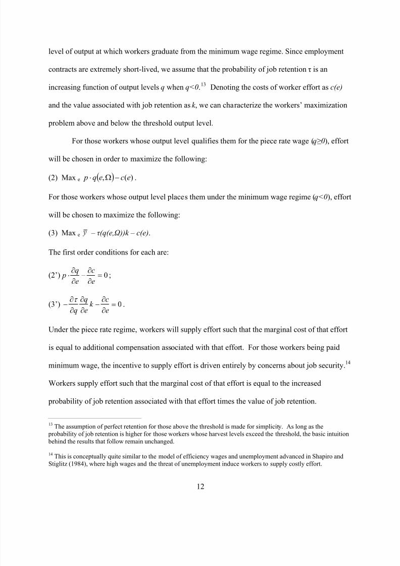
862019 Pllution and Working Effects
httpslidepdfcomreaderfullpllution-and-working-effects 1336
level of output at which workers graduate from the minimum wage regime Since employment
contracts are extremely short-lived we assume that the probability of job retention τ is an
increasing function of output levels q when qlt013
Denoting the costs of worker effort as c(e)
and the value associated with job retention as k we can characterize the workersrsquo maximization
problem above and below the threshold output level
For those workers whose output level qualifies them for the piece rate wage (qge 0) effort
will be chosen in order to maximize the following
(2) Max e ( ) )( eceq p minusΩsdot
For those workers whose output level places them under the minimum wage regime (qlt0) effort
will be chosen to maximize the following
(3) Max e ndash τ (q(eΩ ))k ndash c(e)
The first order conditions for each are
(2rsquo) 0=part
partminus
part
partsdot
e
c
e
q p
(3rsquo) 0=part
partminus
part
part
part
partminus
e
ck
e
q
q
τ
Under the piece rate regime workers will supply effort such that the marginal cost of that effort
is equal to additional compensation associated with that effort For those workers being paid
minimum wage the incentive to supply effort is driven entirely by concerns about job security14
Workers supply effort such that the marginal cost of that effort is equal to the increased
probability of job retention associated with that effort times the value of job retention
13 The assumption of perfect retention for those above the threshold is made for simplicity As long as the probability of job retention is higher for those workers whose harvest levels exceed the threshold the basic intuition behind the results that follow remain unchanged
14 This is conceptually quite similar to the model of efficiency wages and unemployment advanced in Shapiro andStiglitz (1984) where high wages and the threat of unemployment induce workers to supply costly effort
12
862019 Pllution and Working Effects
httpslidepdfcomreaderfullpllution-and-working-effects 1436
The threat of punishment for low levels of output is instrumental in inducing effort under
the minimum wage regime If workers are homogenous and firms set contracts optimally the
gains from job retention due to extra effort will be set equal to the piece rate wage ie
pk q
=part
partminus
τ
such that effort exertion will be identical across both segments of the wage contract
If firms are unable to design optimal contracts effort will differ across regimes Of particular
concern is the situation in which termination incentives are low-powered ie pk q
ltpart
partminus
τ
In
this case workers essentially have a limited liability contract and thus have incentives to shirk
under the minimum wage regime Moreover since the productivity impacts of pollution increase
the probability of workers falling under the minimum wage portion of the compensation scheme
pollution will also indirectly increase the incentive to shirk Accounting for these potentially
different responses to pollution across regimes is central to our econometric model
4 Econometric Model
The worker maximization problem characterized in the previous section suggests the
following econometric model
(4) E[q|Ω X] = P(qge 0|Ω X)E[q|Ω Xqge 0] + (1-P(qge 0|Ω X))E[q|Ω Xqlt0]
where P is the probability a worker has output high enough to place them in the piece rate
regime 1-P is the probability a workerrsquos output places them in the minimum wage regime and X
are other factors that affect productivity (described in more detail below) We are primarily
interested in the direct effect of pollution on productivity (the environmental productivity effect)
Since there is no incentive to shirk in the piece rate regime δq δΩ represents the environmental
13
862019 Pllution and Working Effects
httpslidepdfcomreaderfullpllution-and-working-effects 1536
productivity effect15 To the extent that there is an incentive to shirk in the minimum wage
regime δq δΩ will reflect not only the environmental productivity effect but also the indirect
effect due to the interaction of this pollution effect with shirking incentives
We use two approaches for estimating this equation First we estimate a linear model
using all worker-day observations regardless of output levels and thus the payment regime
obtained that day
(5) q = β olsΩ + θ
ols X + ε
ols
where β ols
is the sum of the direct impact and if it exists the indirect impact of pollution on
productivity If the piece rate contract is set optimally by imposing an appropriate termination
threat as described in the previous section there is no incentive to shirk and β ols
will only
capture the environmental productivity effect To the extent that contracts are not set optimally
and there is an incentive to shirk in the minimum wage regime β ols will instead provide an upper
bound of the estimate of the environmental productivity effect because it will also include the
indirect effect of pollution on productivity via shirking
As a second approach we estimate equation (4) by artificially ldquobottom-codingrdquo our data
and estimating censored regression models To do this we leave all observations in the piece
rate regime as is but assign a measure of productivity of 0 to all observations in the minimum
wage regime16 Thus our estimation strategy can be viewed as a Type I Tobit model of the
following form
(6) q = β cen
Ω + θ cen
X + εcen
q = q if qge 0
15 Although environmental conditions may affect workers they may also have a direct impact on crops While thereis considerable evidence to support that chronic exposure to ozone affects crop yield (eg see Manning 2003) thereis no evidence to support an effect from acute exposure16 Because of our standardization of productivity a value of 0 represents the value when workers switch from theminimum wage to piece rate regime
14
862019 Pllution and Working Effects
httpslidepdfcomreaderfullpllution-and-working-effects 1636
q = 0 if qlt0
where q is the latent measure of productivity Because we are interested in the impact of
pollution on actual productivity which can take on values less than zero the environmental
productivity effect is the marginal effect of pollution on the latent variable q which is simply
β cen
Importantly the actual values of productivity in the minimum wage regime will have no
impact on the likelihood function and hence on β cen That is if shirking occurs so that the
distribution of productivity in the minimum wage regime is shifted to the left these observations
will no longer influence estimates of β cen
because they have been censored Instead only the
observations in the piece rate regime will affect estimates of β
cen
Therefore even if workers are
shirking when paid minimum wage our estimates of β cen
will only capture the environmental
productivity effect
The estimates from these two models can in turn be compared to test for the existence of
shirking If workers shirk when the minimum wage binds then we expect β ols
gt β cen
If workers
do not shirk when the minimum wage binds then we expect β ols
= β cen
We include data from all crops in one regression by using the standardized measures of
productivity described in the data section so the coefficients can be interpreted as a standard
deviation change in productivity from a 1 ppb change in ozone To control for other time-
varying factors that may affect productivity the vector X includes a quadratic in temperature
humidity precipitation wind speed air pressure and solar radiation all measured as the mean
over the typical work-day X also includes a series of day-of-week indicators to capture possible
changes in productivity throughout the week indicator variables for the crop to account for the
mean shift in productivity from different contracts and year-month dummies to control for
trends in pollution and productivity within and across growing seasons All standard errors are
15
862019 Pllution and Working Effects
httpslidepdfcomreaderfullpllution-and-working-effects 1736
two-way clustered on the date because the same environmental conditions are assigned to all
workers on a given day and on the worker to account for serial correlation in worker
productivity
Two facts about how ozone affects health are relevant for the econometric model One
chamber studies which randomly expose a small number of healthy young adults to varying
levels of ozone find that exposure to ozone can affect lung functioning in as quickly as within 1-
2 hours with effects exacerbated by exercise and with continued duration of exposure (see eg
Gong et al 1986 Kulle et al 1985 McDonnell et al 1983) These findings have generally
been confirmed in the field using outdoor workers mail carriers in Taichung City Taiwan and
agricultural workers in Fraser Valley Canada show decrements in lung functioning on days with
higher ozone concentrations (Chan and Wu 2005 Brauer et al 1996) As such we expect the
impact of ozone on productivity to be contemporaneous particularly given the strenuous nature
of this work and duration of exposure Two recovery from ozone pollution is fairly rapid when
removed from exposure Nearly all lung functioning returns to baseline levels in healthy adults
within 24 hours of exposure with recovery taking longer for hyperresponsive adults with
underlying health conditions (Folinsbee and Horvath 1989 Folinsbee and Hazucha 2000)17
Since ozone levels fall considerably overnight as heat and sunlight decline we expect lagged
ozone to have minimal impacts on the productivity of our healthy worker population Given
these two features of the dose-response to ozone we focus our analysis on the contemporaneous
relationship between ozone and productivity Nonetheless we explore the impact of lagged
ozone concentrations in order to confirm that our workers are indeed healthy
17 Although lung functioning recovers after exposure long term damage to lung cells may still occur (Tepper et al1989)
16
862019 Pllution and Working Effects
httpslidepdfcomreaderfullpllution-and-working-effects 1836
5 Results
To test the hypothesis that labor supply is inelastic in the short-run we begin by focusing
on whether work schedules respond to changes in ozone levels We estimate linear regression
models for the decision to work and the number of hours worked (conditional on working) both
with and without worker fixed effects Shown in Table 2 the results in the first two columns
which focus on the decision to work do not support evidence of a labor supply response to
ozone18 The second two columns also reveal that the number of hours worked is not
significantly related to ozone levels Even at the lower 95 confidence interval a 1 ppb increase
in ozone is associated with a 003 drop in hours worked which is a roughly 15 minute decrease
in hours worked The insensitivity of these results to including worker fixed effects strengthens
our confidence in these findings Thus consistent with our contention that avoidance behavior is
not an issue in this setting farm workers do not appear to adjust their work schedules in response
to ozone levels
In Table 3 we present our main results Column (1) presents results from our linear
regression model The estimated coefficient suggests that a 1 ppb increase in ozone leads to a
statistically significant decrease in productivity of 012 of a standard deviation Based on the
distribution of ozone and productivity in our sample this estimate implies that a 10 ppb decrease
in ozone increases worker productivity by 42 percent If wage contracts are set optimally this is
an unbiased estimate of the effect of ozone pollution If contracts are not set optimally and
workers shirk when the minimum wage binds then this estimate will overstate the impact of
ozone In column (2) we show results from a Type I Tobit model where we artificially censor
18 Marginal effects from logit and probit models for the decision to work are virtually identical to the results fromthe linear probability model
17
862019 Pllution and Working Effects
httpslidepdfcomreaderfullpllution-and-working-effects 1936
observations when the minimum wage binds and find an identical 012 standard deviation effect
from a 1 ppb change in ozone
Since this Tobit model assumes normality and homoskedasticity we assess the sensitivity
of our results to these assumptions by estimating a censored median regression model also
displaying results from an uncensored median regression model as a reference point19
Shown in
column (3) the median regression estimate is quite comparable to the linear regression estimate
which is not surprising given the distribution of productivity shown in Figure 1 The censored
median regression results shown in column (4) are also quite similar to the estimates from the
parametric censored models lending support to the parametric assumptions The comparability
of the four estimates in this Table suggests that shirking due to the minimum wage is relatively
minimal in this setting Thus the basic linear regression specification appears to yield unbiased
estimates of the pollution productivity effect
Although the lack of shirking in the minimum wage regime may appear surprising as
discussed in the conceptual framework this can arise if the gains from job retention associated
with providing effort are sufficiently large This is particularly important in our setting where
output is easily verified and labor contracts are extremely short-lived In order to examine the
potential importance of these features we provide descriptive evidence on the relationship
between worker productivity and separations We define a separation as the last day we observe
a worker in the data Similar to Lazear (2000) Table 4 shows the rate of separation by decile of
daily productivity Immediately evident is that less productive workers are more likely to
experience separations 65 percent of workers whose productivity falls in the bottom decile on
any given day separate from the farm while only 25 percent in the top decile separate (this
difference is statistically significant) As the next column shows highly productive workers
19 We estimate a censored median model using the 3-step procedure developed by Chernozhukov and Hong (2002)
18
862019 Pllution and Working Effects
httpslidepdfcomreaderfullpllution-and-working-effects 2036
typically have more tenure so some of these differences in separations could be driven by
differences in tenure In column (3) we show separations by productivity after adjusting for the
impact of tenure on productivity and find quite similar results Although we can not identify the
reason for a separation these results are consistent with the idea that the threat of termination for
less productive workers is reasonably high in this setting
In Table 5 we explore the sensitivity of both our linear and Tobit estimates to various
additional assumptions Column (1) repeats the baseline results In column (2) we include
worker fixed effects Although this increases the explanatory power of our regressions
considerably the estimates for ozone are largely unchanged consistent with the notion that
workers are not selecting into employment on any given day based on ozone concentrations
Since ozone is formed in part because of temperature and sunlight it is essential that we
properly control for these variables While we already control for a quadratic in mean
temperature and solar radiation we explore the sensitivity of the ozone estimates by also
including daily minimum and maximum temperature and solar radiation (column 3) and by
controlling for all three temperature measures more flexibly by using a series of indicator
variables for every 5 degrees Fahrenheit instead of a quadratic (column 4) Our estimates for
ozone remain largely unaffected by these changes suggesting that although ozone and
temperature are highly correlated the quadratic in mean temperature in our main specification
adequately controls for temperature
Figure 1 provided some evidence that worker effort changes near the regime threshold
particularly for crop 1 where contracts are time plus all pieces If higher ozone levels reduce
productivity and hence make it more likely for workers to fall into the minimum wage regime
this offsetting increase in effort may bias our results down In the remaining two columns of
19
862019 Pllution and Working Effects
httpslidepdfcomreaderfullpllution-and-working-effects 2136
Table 5 we address this by excluding observations that are close to the regime threshold varying
our definition of ldquocloserdquo20 Consistent with expectations our results are slightly larger as we
exclude more observations but these differences are minimal
To address potential concerns about the cumulative effect of ozone exposure we also
present results that include 1 and 2-day lags of ozone Since ozone levels may only reflect
exposure on days when workers actually work we limit our focus to days when workers have
worked the previous day by excluding from our analysis the first one or two days of the
workweek depending on how many lags we include in our specification Table 6 column (1)
repeats our baseline results from the linear regression model Shown in column (2) are results
without any lags but excluding Monday which are slightly higher than the baseline results
Including 1 lag of ozone shown in column (3) we find that the coefficient on contemporaneous
ozone remains the same and lagged ozone is negative but statistically insignificant The results
in column (4) show that excluding the first two work days continues to increase the
contemporaneous coefficient on ozone Including two lags of ozone column (5) shows that the
coefficient on contemporaneous ozone remains statistically significant and again unchanged
while both lags of ozone are statistically insignificant Together these estimates suggest that the
predominant effect of ozone is from same day exposure with an overnight respite from ozone
sufficient for lung functioning to return to baseline levels Moreover this rapid recovery implies
that the environmental productivity effects measured in this paper are predominantly impacting a
healthy population21
20 We also estimated models that completely excluded observations under the time plus all pieces contract and our estimates for ozone were -010 for the linear model and -013 for the Tobit model which are largely the same asthose found when those observations were included21 Recall from Section 4 that chamber studies suggest a rapid recovery from ozone exposure for healthy individuals
20
862019 Pllution and Working Effects
httpslidepdfcomreaderfullpllution-and-working-effects 2236
6 Conclusion
In this paper we merge a unique dataset on individual-level daily harvest rates for
agricultural workers with data on environmental conditions to assess the impact of ozone
pollution on worker productivity We find that a 10 ppb change in average ozone exposure
results in a significant and robust 42 percent change in agricultural worker productivity Despite
the applicability of minimum wages and the incentive to shirk we find little evidence of
differential effects depending on whether or not the minimum wage binds Importantly this
environmental productivity effect suggests that common characterizations of environmental
protection as purely a tax on producers and consumers to be weighed against the consumption
benefits associated with improved environmental quality may be misguided Environmental
protection can also be viewed as an investment in human capital and its contribution to firm
productivity and economic growth should be incorporated in the calculus of policy makers
Our results also speak to the ongoing debates on ozone policy Ozone pollution
continues to be a pervasive environmental issue throughout much of the world Debates over the
optimal level of ozone have ensued for many years and current efforts to strengthen these
standards remain contentious Defining regulatory thresholds depends in part on the benefits
associated with avoided exposure which has traditionally been estimated through a focus on
high-visibility health effects such as hospitalizations The labor productivity impacts measured
in this paper help make these benefits calculations more complete Our results indicate that
ozone even at levels below current air quality standards in most of the world has significant
negative impacts on worker productivity suggesting that the strengthening of regulations on
ozone pollution would yield additional benefits
21
862019 Pllution and Working Effects
httpslidepdfcomreaderfullpllution-and-working-effects 2336
These impacts of ozone on agricultural workers are also important in their own right A
back-of-the envelope calculation that applies the environmental productivity effect estimated in
the Central Valley of California to the whole of the US suggests that a 10 ppb reduction in the
ozone standard would translate into an annual cost savings of approximately $11 billion in labor
expenditure22
In the developing world where national incomes depend more heavily on
agriculture these productivity effects are likely to have a much larger impact on the economy
These impacts may be especially large in countries like India China and Mexico where rapid
industrial growth and automobile penetration contribute precursor chemicals that contribute to
substantially higher levels of ozone pollution
While the impacts of ozone on agricultural productivity are large the generalizability of
these findings to other pollutants and industries is unclear Agricultural workers face
considerably higher levels of exposure to pollution than individuals who work indoors That
said roughly 118 percent of the US labor force works in an industry with regular exposure to
outdoor conditions and this figure is much higher for middle- and lower-income countries (Graff
Zivin and Neidell 2010) Moreover many forms of outdoor pollution diminish indoor air
quality as well For example indoor penetration of fine particulate matter ranges from 38-94
for typical residential homes in the US (Abt et al 2000) Examining the generalizability of the
environmental productivity effect estimated in this paper to other pollutants and industries
represents a fruitful area for future research
22 Total labor expenditure in US agriculture was approximately $265B in 2007 (USDA 2009)
22
862019 Pllution and Working Effects
httpslidepdfcomreaderfullpllution-and-working-effects 2436
References
Abt Eileen Helen H Suh Paul Catalano and Petros Koutrakis (2000) ldquoRelative Contributionof Outdoor and Indoor Particle Sources to Indoor Concentrationsrdquo Environmental Science and Technology 34 (17) pp 3579ndash3587
Auffhammer Maximilian and Ryan Kellogg (2011) ldquoClearing the Air The Effects of GasolineContent Regulation on Air Qualityrdquo American Economic Review forthcoming
Bandiera Oriana Iwan Barankay and Imran Rasul (2005) ldquoSocial Preferences and theResponse to Incentives Evidence from Personnel Datardquo Quarterly Journal of Economics
120(3) 917-962
Bandiera Oriana Iwan Barankay and Imran Rasul (2010) ldquoSocial Incentives in theWorkplacerdquo Review of Economic Studies 77(2) 417-458
Banzhaf H Spencer and Randall Walsh (2008) ldquoDo People Vote with Their Feet AnEmpirical Test of Tieboutrdquo American Economic Review 98(3) 843ndash63
Bell Michelle Aidan McDermott Scott Zeger Jonathan Samet Francesca Dominici (2004)ldquoOzone and Short-term Mortality in 95 US Urban Communities 1987-2000rdquo Journal of the American Medical Association 292 (19)
Blanchard Charles and Shelley Tanenbaum (2003) ldquoDifferences between Weekday andWeekend Air Pollutant Levels in Southern Californiardquo Journal of the Air and Waste
Management Association 53(7)
Brauer M and JR Brook (1995) ldquoPersonal and Fixed-Site Ozone Measurementswith a Passive Samplerrdquo Journal of the Air and Waste Management Association 45 (7) 529-537
Brauer M J Blair and S Vedal (1996) ldquoEffect of ambient ozone exposure on lung function infarm workersrdquo Am J Respir Crit Care Med 154(4) 981-987
Carson Richard Phoebe Koundouri and Ceacuteline Nauges (2010) ldquoArsenic Mitigation inBangladesh A Household Labor Market Approachrdquo American Journal of Agricultural Economics 92
Chan Chang-Chuan and Tsung-Huan Wu (2005) ldquoEffects of Ambient Ozone Exposure on MailCarriers Peak Expiratory Flow Ratesrdquo Environmental Health Perspectives 113(6) 735-738
Chay Kenneth and Michael Greenstone (2003) ldquoThe Impact of Air Pollution on InfantMortality Evidence from Geographic Variation in Pollution Shocks Induced by a RecessionrdquoQuarterly Journal of Economics 118(3) 1121-1167
23
862019 Pllution and Working Effects
httpslidepdfcomreaderfullpllution-and-working-effects 2536
Chay Kenneth and Michael Greenstone (2005) ldquoDoes Air Quality Matter Evidence from theHousing Marketrdquo Journal of Political Economy 113 376ndash424
Chernozhukov Victor and Han Hong (2002) ldquoThree-step censored quantile regression andextramarital affairsrdquo Journal of the American Statistical Association 97(459) 872-882
Currie Janet and Matthew Neidell (2005) ldquoAir Pollution and Infant Health What Can We Learnfrom Californias Recent Experiencerdquo Quarterly Journal of Economics 120(3) 1003-1030
Dockery Douglas W C Arden Pope Xiping Xu John D Spengler James H Ware Martha EFay Benjamin G Ferris and Frank E Speizer (1993) ldquoAn association between air pollution andmortality in six US citiesrdquo The New England Journal of Medicine 3291753-1759
Environmental Protection Agency (2010) ldquoNational Ambient Air Quality Standards for Ozone(Proposed Rule)rdquo Federal Register 7511 (January 19 2010) p 2938-3052
Folinsbee L J Hazucha M J (2000) ldquoTime course of response to ozone exposure in healthyadult femalesrdquo Inhalation Toxicol 12 151-167
Folinsbee L J Horvath S M (1986) ldquoPersistence of the acute effects of ozone exposurerdquo Aviat Space Environ Med 57 1136-1143
Gong H Jr Bradley P W Simmons M S Tashkin D P (1986) ldquoImpaired exercise performance and pulmonary function in elite cyclists during low-level ozone exposure in a hotenvironmentrdquo Am Rev Respir Dis 134 726-733
Graff Zivin Joshua and Matthew Neidell (2010) ldquoTemperature and the allocation of timeImplications for climate changerdquo NBER working paper 15717
Hanna Rema and Paulina Oliva (2011) ldquoThe Effect of Pollution on Labor Supply Evidencefrom a Natural Experiment in Mexico Cityrdquo Mimeo
Hazucha M J LJ Folinsbee and PA Bromberg (2003) ldquoDistribution and reproducibility of spirometric response to ozone by gender and agerdquo J Appl Physiol 95 1917-1925
Hausman Jerry Bart Ostro and David Wise (1984) ldquoAir Pollution and Lost Workrdquo NBER Working Paper No 1263
Kulle T J Sauder L R Hebel J R Chatham M D (1985) rdquoOzone response relationshipsin healthy nonsmokersrdquo Am Rev Respir Dis 132 36-41
Lazear Edward (2000) ldquoPerformance pay and productivityrdquo American Economic Review 90(5)1346-1361
24
862019 Pllution and Working Effects
httpslidepdfcomreaderfullpllution-and-working-effects 2636
Manning WJ (2003) ldquoAssessing plant responses to ambient ozone Growth of ozone-sensitiveloblolly pine seedlings treated with ethylenediurea (EDU) and sodium erythorbate (NaE)rdquo Environ Pollut 126(1) 73-81
McDonnell W F Horstman D H Hazucha M J Seal E Jr Haak E D Salaam S A
House D E (1983) ldquoPulmonary effects of ozone exposure during exercise dose-responsecharacteristicsrdquo J Appl Physiol Respir Environ Exercise Physiol 54 1345-1352
Neidell Matthew (2009) ldquoInformation Avoidance Behavior and Health The Effect of Ozoneon Asthma Hospitalizationsrdquo Journal of Human Resources 44(2)
ONeill MS Ramirez-Aguilar M Meneses-Gonzalez F Hernaacutendez-Avila M Geyh AS Sienra-Monge JJ Romieu I (2003) ldquoOzone exposure among Mexico City outdoor workersrdquo J Air
Waste Manag Assoc 53(3) 339-46
Ostro Bart (1983) ldquoThe Effects of Air Pollution on Work Lost and Morbidity Journal of
Environmental Economics and Management 10(4) 371-382
Paarsch Harry J and Bruce Shearer (1999) ldquoThe Response of Worker Effort to Piece RatesEvidence from the British Columbia Tree-Planting Industry Journal of Human Resources 34643-667
Paarsch Harry J and Bruce Shearer (2000) ldquoPiece Rates Fixed Wages and Incentive EffectsStatistical Evidence from Payroll Records International Economic Review 40 59-92
Pope CA III Burnett RT Thun MJ Calle EE Krewski D Ito K Thurston GD (2002) ldquoLungCancer Cardiopulmonary Mortality and Long-term Exposure to Fine Particulate Air Pollutionrdquo Journal of the American Medical Association 2871132-1141
Shapiro Carl and Joseph Stiglitz (1984) ldquoEquilibrium unemployment as a worker disciplinedevicerdquo American Economic Review 74(3)
Shi Lan (2010) ldquoIncentive Effect of Piece Rate Contracts Evidence from Two Small FieldExperimentsrdquo The BE Journal of Economic Analysis amp Policy 10(1) (Topics)
Sillman Sanford (1999) ldquoThe Relation Between Ozone NOx and Hydrocarbons in Urban andPolluted Rural Environmentsrdquo Atmospheric Environment 33 1821-1845
Tepper J S Costa D L Lehmann J R Weber M F Hatch G E (1989) ldquoUnattenuatedstructural and biochemical alterations in the rat lung during functional adaptation to ozonerdquo Am
Rev Respir Dis 140 493-501
USDA (2009) 2007 Census of Agriculture (AC-07-A-5) National Agricultural StatisticsService Washington DC
25
862019 Pllution and Working Effects
httpslidepdfcomreaderfullpllution-and-working-effects 2736
Figure 1 Standardized average hourly pieces collected by crop and for all crops
Notes We standardize average hourly productivity by subtracting the minimum number of pieces per hour requiredto reach the piece rate regime and dividing by the standard deviation of productivity for each crop The vertical linereflects the regime threshold for crossing from the minimum wage to the piece rate regime
0
2
4
6
0
2
4
6
-5 0 5 -5 0 5
Crop 1 (time+all pieces) Crop 2 (time+pieces $03p)
Crop 3 (time+pieces $1p) Total
D e n s i t y
26
862019 Pllution and Working Effects
httpslidepdfcomreaderfullpllution-and-working-effects 2836
Figure 2 Variation in productivity by worker all crops
0
1
2
3
4
5
D e n s i t y
-4 -2 0 2
27
862019 Pllution and Working Effects
httpslidepdfcomreaderfullpllution-and-working-effects 2936
Figure 3 Variation in productivity by day all crops
0
2
4
6
D e n s i t y
-3 -2 -1 0 1 2
28
862019 Pllution and Working Effects
httpslidepdfcomreaderfullpllution-and-working-effects 3036
Figure 4 Average demeaned daily ozone and temperature in 2010
-40
-30
-20
-10
0
10
20
30
40
50
512010 612010 712010 812010 912010 1012010
d e m e a n e d v a l u e
ozone temperature harves t day
29
862019 Pllution and Working Effects
httpslidepdfcomreaderfullpllution-and-working-effects 3136
Table 1 Summary statistics
A Productivity variables (n=36215)Observations mean SD SD within
worker SD between
workers
1 Minimum wage regimeHourly pieces (crop 1) 11753 203 057 044 047Hourly pieces (crop 2) 4114 308 077 065 069Hourly pieces (crop 3) 5920 229 048 031 044hours worked 21787 763 129 076 1202 Piece rate regimeHourly pieces (crop 1) 3675 342 040 030 032Hourly pieces (crop 2) 5512 492 085 061 064Hourly pieces (crop 3) 5241 388 082 050 066hours worked 14428 734 152 096 135
B Environmental variables (n=155)mean SD min maxozone (ppb) 4777 1324 1050 8600temperature (F) 7815 852 5630 9698atmospheric pressure (mb) 100155 648 98886 101259resultant wind speed (mph) 274 053 161 460solar radiation (Wm2) 83733 17407 18700 108333relative humidity () 4533 1004 2790 9350 precipitation (mm) 240 505 000 3548
C Sample
total of dates 155total of employees 1664mean of days with farm 20
Notes SD Standard deviation Crop 1 is time plus all pieces with a piece rate of $05piece and minimum pieces per hour of 3 Crop 2 is time plus pieces with a piece rate of $03piece and minimum pieces per hour of 4 Crop 3 istime plus pieces with a piece rate of $1piece and minimum pieces per hour of 3
30
862019 Pllution and Working Effects
httpslidepdfcomreaderfullpllution-and-working-effects 3236
Table 2 Regression results of the effect of ozone on avoidance behavior
1 2 3 4
extensive margin probability(work)
intensive margin hours worked
ozone (ppb) -00017 -00018 00014 00014[00020] [00021] [00123] [00125]worker fixed effect N Y N YObservations 39223 39223 36215 36215R-squared 011 016 024 027Standard errors clustered on date and worker in brackets significant at 10 significant at 5 significantat 1 All regressions include controls for temperature (quadratic) air pressure wind speed solar radiation relativehumidity precipitation day of week dummies monthyear dummies and piece rate contract type dummies Allenvironmental variables are the mean of hourly values from 6am-3pm
31
862019 Pllution and Working Effects
httpslidepdfcomreaderfullpllution-and-working-effects 3336
Table 3 Main regression results of the effect of ozone on productivity
1 2 3 4
ozone (ppb) -00116 -00123 -00092 -00124[00043] [00052] [00055] [00058]
model linear Tobit median censoredmedianObservations 36215 36215 36215 36215(Psuedo) R2 031 010 019 024Standard errors clustered on date and worker in brackets significant at 10 significant at 5 significantat 1 The dependent variable is standardized hourly pieces collected All regressions include controls for temperature (quadratic) air pressure wind speed solar radiation relative humidity precipitation day of week dummies monthyear dummies and piece rate contract type dummies All environmental variables are the mean of hourly values from 6am-3pm Bootstrapped standard errors for both median regressions were obtained using 50replications
32
862019 Pllution and Working Effects
httpslidepdfcomreaderfullpllution-and-working-effects 3436
Table 4 Separation rates by productivity decile
1 2 3 4
A Unadjusted productivity B Productivity adjusted for tenure
productivitydecile separation rate tenure (days) separation rate tenure (days)
1 0065 1244 0061 17992 0060 1555 0063 19203 0047 1658 0055 18474 0053 1896 0047 19475 0034 1864 0047 21566 0042 2128 0039 22137 0044 2109 0038 19248 0032 2227 0029 18729 0025 2324 0024 1941
10 0025 2431 0023 1817This table shows daily mean separation rates and tenure by productivity decile
33
862019 Pllution and Working Effects
httpslidepdfcomreaderfullpllution-and-working-effects 3536
Table 5 Sensitivity of regression results of the effect of ozone on productivity
1 2 3 4 5 6
A Linear model
ozone (ppb) -00116 -00097 -00125 -00111 -00129 -00136
[00043] [00041] [00045] [00050] [00048] [00052]R-squared 031 053 031 033 032 033
B Tobit model
ozone (ppb) -00123 -00105 -00121 -00130 -00146 -00154[00052] [00049] [00053] [00059] [00057] [00064]
Pseudo R-squared
010 031 010 011 012 013
model baseline worker fixed
effect
includemin and
max of temp(quadratic)and solar
rad
includemin and
max of temp(indicators)and solar
rad
excludeobs 1 SD
of regimethreshold
excludeobs 2 SD
of regimethreshold
Observations 36215 36215 36215 36215 32415 30239Standard errors clustered on date and worker in brackets significant at 10 significant at 5 significantat 1 The dependent variable is standardized hourly pieces collected All regressions include controls for temperature (quadratic except column 4 which includes indicator variables for every 5 degrees F) air pressurewind speed solar radiation relative humidity precipitation day of week dummies monthyear dummies and piecerate contract type dummies All environmental variables are based on hourly values from 6am-3pm
34
862019 Pllution and Working Effects
httpslidepdfcomreaderfullpllution-and-working-effects 3636
Table 6 Regression results of the effect of lagged ozone on productivity
1 2 3 4 5
A Linear model
ozone (ppb) -0011 -0013 -0013 -0016 -0015
[0004] [0005] [0005] [0005] [0005]1 lag ozone (ppb) -0004 -0006[0004] [0006]
2 lag ozone (ppb) 0003[0005]
R-squared 031 032 032 032 032
B Tobit model
ozone (ppb) -0012 -0013 -0012 -0016 -0014[0005] [0006] [0006] [0006] [0006]
1 lag ozone (ppb) -0003 -0003
[0005] [0007]2 lag ozone (ppb) 0001[0005]
Pseudo R-squared 010 010 010 010 010
Day(s) of week excluded
none Monday Monday Monday ampTuesday
Monday ampTuesday
Observations 35465 25456 25456 17498 17498Standard errors clustered on date and worker in brackets significant at 10 significant at 5 significantat 1 The dependent variable is standardized hourly pieces collected All regressions control for temperature(quadratic) air pressure wind speed solar radiation relative humidity precipitation day of week dummiesmonthyear dummies and piece rate contract type dummies All environmental variables are the mean of hourly
values from 6am-3pm
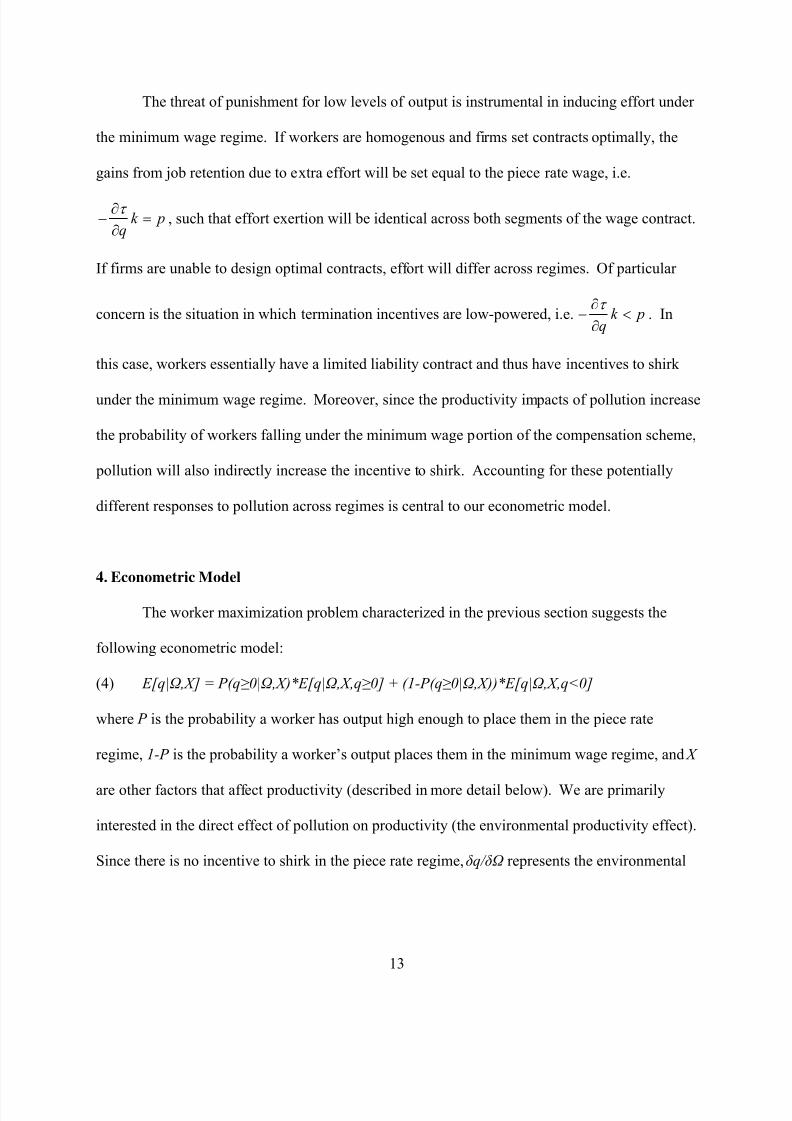
862019 Pllution and Working Effects
httpslidepdfcomreaderfullpllution-and-working-effects 1636
q = 0 if qlt0
where q is the latent measure of productivity Because we are interested in the impact of
pollution on actual productivity which can take on values less than zero the environmental
productivity effect is the marginal effect of pollution on the latent variable q which is simply
β cen
Importantly the actual values of productivity in the minimum wage regime will have no
impact on the likelihood function and hence on β cen That is if shirking occurs so that the
distribution of productivity in the minimum wage regime is shifted to the left these observations
will no longer influence estimates of β cen
because they have been censored Instead only the
observations in the piece rate regime will affect estimates of β
cen
Therefore even if workers are
shirking when paid minimum wage our estimates of β cen
will only capture the environmental
productivity effect
The estimates from these two models can in turn be compared to test for the existence of
shirking If workers shirk when the minimum wage binds then we expect β ols
gt β cen
If workers
do not shirk when the minimum wage binds then we expect β ols
= β cen
We include data from all crops in one regression by using the standardized measures of
productivity described in the data section so the coefficients can be interpreted as a standard
deviation change in productivity from a 1 ppb change in ozone To control for other time-
varying factors that may affect productivity the vector X includes a quadratic in temperature
humidity precipitation wind speed air pressure and solar radiation all measured as the mean
over the typical work-day X also includes a series of day-of-week indicators to capture possible
changes in productivity throughout the week indicator variables for the crop to account for the
mean shift in productivity from different contracts and year-month dummies to control for
trends in pollution and productivity within and across growing seasons All standard errors are
15
862019 Pllution and Working Effects
httpslidepdfcomreaderfullpllution-and-working-effects 1736
two-way clustered on the date because the same environmental conditions are assigned to all
workers on a given day and on the worker to account for serial correlation in worker
productivity
Two facts about how ozone affects health are relevant for the econometric model One
chamber studies which randomly expose a small number of healthy young adults to varying
levels of ozone find that exposure to ozone can affect lung functioning in as quickly as within 1-
2 hours with effects exacerbated by exercise and with continued duration of exposure (see eg
Gong et al 1986 Kulle et al 1985 McDonnell et al 1983) These findings have generally
been confirmed in the field using outdoor workers mail carriers in Taichung City Taiwan and
agricultural workers in Fraser Valley Canada show decrements in lung functioning on days with
higher ozone concentrations (Chan and Wu 2005 Brauer et al 1996) As such we expect the
impact of ozone on productivity to be contemporaneous particularly given the strenuous nature
of this work and duration of exposure Two recovery from ozone pollution is fairly rapid when
removed from exposure Nearly all lung functioning returns to baseline levels in healthy adults
within 24 hours of exposure with recovery taking longer for hyperresponsive adults with
underlying health conditions (Folinsbee and Horvath 1989 Folinsbee and Hazucha 2000)17
Since ozone levels fall considerably overnight as heat and sunlight decline we expect lagged
ozone to have minimal impacts on the productivity of our healthy worker population Given
these two features of the dose-response to ozone we focus our analysis on the contemporaneous
relationship between ozone and productivity Nonetheless we explore the impact of lagged
ozone concentrations in order to confirm that our workers are indeed healthy
17 Although lung functioning recovers after exposure long term damage to lung cells may still occur (Tepper et al1989)
16
862019 Pllution and Working Effects
httpslidepdfcomreaderfullpllution-and-working-effects 1836
5 Results
To test the hypothesis that labor supply is inelastic in the short-run we begin by focusing
on whether work schedules respond to changes in ozone levels We estimate linear regression
models for the decision to work and the number of hours worked (conditional on working) both
with and without worker fixed effects Shown in Table 2 the results in the first two columns
which focus on the decision to work do not support evidence of a labor supply response to
ozone18 The second two columns also reveal that the number of hours worked is not
significantly related to ozone levels Even at the lower 95 confidence interval a 1 ppb increase
in ozone is associated with a 003 drop in hours worked which is a roughly 15 minute decrease
in hours worked The insensitivity of these results to including worker fixed effects strengthens
our confidence in these findings Thus consistent with our contention that avoidance behavior is
not an issue in this setting farm workers do not appear to adjust their work schedules in response
to ozone levels
In Table 3 we present our main results Column (1) presents results from our linear
regression model The estimated coefficient suggests that a 1 ppb increase in ozone leads to a
statistically significant decrease in productivity of 012 of a standard deviation Based on the
distribution of ozone and productivity in our sample this estimate implies that a 10 ppb decrease
in ozone increases worker productivity by 42 percent If wage contracts are set optimally this is
an unbiased estimate of the effect of ozone pollution If contracts are not set optimally and
workers shirk when the minimum wage binds then this estimate will overstate the impact of
ozone In column (2) we show results from a Type I Tobit model where we artificially censor
18 Marginal effects from logit and probit models for the decision to work are virtually identical to the results fromthe linear probability model
17
862019 Pllution and Working Effects
httpslidepdfcomreaderfullpllution-and-working-effects 1936
observations when the minimum wage binds and find an identical 012 standard deviation effect
from a 1 ppb change in ozone
Since this Tobit model assumes normality and homoskedasticity we assess the sensitivity
of our results to these assumptions by estimating a censored median regression model also
displaying results from an uncensored median regression model as a reference point19
Shown in
column (3) the median regression estimate is quite comparable to the linear regression estimate
which is not surprising given the distribution of productivity shown in Figure 1 The censored
median regression results shown in column (4) are also quite similar to the estimates from the
parametric censored models lending support to the parametric assumptions The comparability
of the four estimates in this Table suggests that shirking due to the minimum wage is relatively
minimal in this setting Thus the basic linear regression specification appears to yield unbiased
estimates of the pollution productivity effect
Although the lack of shirking in the minimum wage regime may appear surprising as
discussed in the conceptual framework this can arise if the gains from job retention associated
with providing effort are sufficiently large This is particularly important in our setting where
output is easily verified and labor contracts are extremely short-lived In order to examine the
potential importance of these features we provide descriptive evidence on the relationship
between worker productivity and separations We define a separation as the last day we observe
a worker in the data Similar to Lazear (2000) Table 4 shows the rate of separation by decile of
daily productivity Immediately evident is that less productive workers are more likely to
experience separations 65 percent of workers whose productivity falls in the bottom decile on
any given day separate from the farm while only 25 percent in the top decile separate (this
difference is statistically significant) As the next column shows highly productive workers
19 We estimate a censored median model using the 3-step procedure developed by Chernozhukov and Hong (2002)
18
862019 Pllution and Working Effects
httpslidepdfcomreaderfullpllution-and-working-effects 2036
typically have more tenure so some of these differences in separations could be driven by
differences in tenure In column (3) we show separations by productivity after adjusting for the
impact of tenure on productivity and find quite similar results Although we can not identify the
reason for a separation these results are consistent with the idea that the threat of termination for
less productive workers is reasonably high in this setting
In Table 5 we explore the sensitivity of both our linear and Tobit estimates to various
additional assumptions Column (1) repeats the baseline results In column (2) we include
worker fixed effects Although this increases the explanatory power of our regressions
considerably the estimates for ozone are largely unchanged consistent with the notion that
workers are not selecting into employment on any given day based on ozone concentrations
Since ozone is formed in part because of temperature and sunlight it is essential that we
properly control for these variables While we already control for a quadratic in mean
temperature and solar radiation we explore the sensitivity of the ozone estimates by also
including daily minimum and maximum temperature and solar radiation (column 3) and by
controlling for all three temperature measures more flexibly by using a series of indicator
variables for every 5 degrees Fahrenheit instead of a quadratic (column 4) Our estimates for
ozone remain largely unaffected by these changes suggesting that although ozone and
temperature are highly correlated the quadratic in mean temperature in our main specification
adequately controls for temperature
Figure 1 provided some evidence that worker effort changes near the regime threshold
particularly for crop 1 where contracts are time plus all pieces If higher ozone levels reduce
productivity and hence make it more likely for workers to fall into the minimum wage regime
this offsetting increase in effort may bias our results down In the remaining two columns of
19
862019 Pllution and Working Effects
httpslidepdfcomreaderfullpllution-and-working-effects 2136
Table 5 we address this by excluding observations that are close to the regime threshold varying
our definition of ldquocloserdquo20 Consistent with expectations our results are slightly larger as we
exclude more observations but these differences are minimal
To address potential concerns about the cumulative effect of ozone exposure we also
present results that include 1 and 2-day lags of ozone Since ozone levels may only reflect
exposure on days when workers actually work we limit our focus to days when workers have
worked the previous day by excluding from our analysis the first one or two days of the
workweek depending on how many lags we include in our specification Table 6 column (1)
repeats our baseline results from the linear regression model Shown in column (2) are results
without any lags but excluding Monday which are slightly higher than the baseline results
Including 1 lag of ozone shown in column (3) we find that the coefficient on contemporaneous
ozone remains the same and lagged ozone is negative but statistically insignificant The results
in column (4) show that excluding the first two work days continues to increase the
contemporaneous coefficient on ozone Including two lags of ozone column (5) shows that the
coefficient on contemporaneous ozone remains statistically significant and again unchanged
while both lags of ozone are statistically insignificant Together these estimates suggest that the
predominant effect of ozone is from same day exposure with an overnight respite from ozone
sufficient for lung functioning to return to baseline levels Moreover this rapid recovery implies
that the environmental productivity effects measured in this paper are predominantly impacting a
healthy population21
20 We also estimated models that completely excluded observations under the time plus all pieces contract and our estimates for ozone were -010 for the linear model and -013 for the Tobit model which are largely the same asthose found when those observations were included21 Recall from Section 4 that chamber studies suggest a rapid recovery from ozone exposure for healthy individuals
20
862019 Pllution and Working Effects
httpslidepdfcomreaderfullpllution-and-working-effects 2236
6 Conclusion
In this paper we merge a unique dataset on individual-level daily harvest rates for
agricultural workers with data on environmental conditions to assess the impact of ozone
pollution on worker productivity We find that a 10 ppb change in average ozone exposure
results in a significant and robust 42 percent change in agricultural worker productivity Despite
the applicability of minimum wages and the incentive to shirk we find little evidence of
differential effects depending on whether or not the minimum wage binds Importantly this
environmental productivity effect suggests that common characterizations of environmental
protection as purely a tax on producers and consumers to be weighed against the consumption
benefits associated with improved environmental quality may be misguided Environmental
protection can also be viewed as an investment in human capital and its contribution to firm
productivity and economic growth should be incorporated in the calculus of policy makers
Our results also speak to the ongoing debates on ozone policy Ozone pollution
continues to be a pervasive environmental issue throughout much of the world Debates over the
optimal level of ozone have ensued for many years and current efforts to strengthen these
standards remain contentious Defining regulatory thresholds depends in part on the benefits
associated with avoided exposure which has traditionally been estimated through a focus on
high-visibility health effects such as hospitalizations The labor productivity impacts measured
in this paper help make these benefits calculations more complete Our results indicate that
ozone even at levels below current air quality standards in most of the world has significant
negative impacts on worker productivity suggesting that the strengthening of regulations on
ozone pollution would yield additional benefits
21
862019 Pllution and Working Effects
httpslidepdfcomreaderfullpllution-and-working-effects 2336
These impacts of ozone on agricultural workers are also important in their own right A
back-of-the envelope calculation that applies the environmental productivity effect estimated in
the Central Valley of California to the whole of the US suggests that a 10 ppb reduction in the
ozone standard would translate into an annual cost savings of approximately $11 billion in labor
expenditure22
In the developing world where national incomes depend more heavily on
agriculture these productivity effects are likely to have a much larger impact on the economy
These impacts may be especially large in countries like India China and Mexico where rapid
industrial growth and automobile penetration contribute precursor chemicals that contribute to
substantially higher levels of ozone pollution
While the impacts of ozone on agricultural productivity are large the generalizability of
these findings to other pollutants and industries is unclear Agricultural workers face
considerably higher levels of exposure to pollution than individuals who work indoors That
said roughly 118 percent of the US labor force works in an industry with regular exposure to
outdoor conditions and this figure is much higher for middle- and lower-income countries (Graff
Zivin and Neidell 2010) Moreover many forms of outdoor pollution diminish indoor air
quality as well For example indoor penetration of fine particulate matter ranges from 38-94
for typical residential homes in the US (Abt et al 2000) Examining the generalizability of the
environmental productivity effect estimated in this paper to other pollutants and industries
represents a fruitful area for future research
22 Total labor expenditure in US agriculture was approximately $265B in 2007 (USDA 2009)
22
862019 Pllution and Working Effects
httpslidepdfcomreaderfullpllution-and-working-effects 2436
References
Abt Eileen Helen H Suh Paul Catalano and Petros Koutrakis (2000) ldquoRelative Contributionof Outdoor and Indoor Particle Sources to Indoor Concentrationsrdquo Environmental Science and Technology 34 (17) pp 3579ndash3587
Auffhammer Maximilian and Ryan Kellogg (2011) ldquoClearing the Air The Effects of GasolineContent Regulation on Air Qualityrdquo American Economic Review forthcoming
Bandiera Oriana Iwan Barankay and Imran Rasul (2005) ldquoSocial Preferences and theResponse to Incentives Evidence from Personnel Datardquo Quarterly Journal of Economics
120(3) 917-962
Bandiera Oriana Iwan Barankay and Imran Rasul (2010) ldquoSocial Incentives in theWorkplacerdquo Review of Economic Studies 77(2) 417-458
Banzhaf H Spencer and Randall Walsh (2008) ldquoDo People Vote with Their Feet AnEmpirical Test of Tieboutrdquo American Economic Review 98(3) 843ndash63
Bell Michelle Aidan McDermott Scott Zeger Jonathan Samet Francesca Dominici (2004)ldquoOzone and Short-term Mortality in 95 US Urban Communities 1987-2000rdquo Journal of the American Medical Association 292 (19)
Blanchard Charles and Shelley Tanenbaum (2003) ldquoDifferences between Weekday andWeekend Air Pollutant Levels in Southern Californiardquo Journal of the Air and Waste
Management Association 53(7)
Brauer M and JR Brook (1995) ldquoPersonal and Fixed-Site Ozone Measurementswith a Passive Samplerrdquo Journal of the Air and Waste Management Association 45 (7) 529-537
Brauer M J Blair and S Vedal (1996) ldquoEffect of ambient ozone exposure on lung function infarm workersrdquo Am J Respir Crit Care Med 154(4) 981-987
Carson Richard Phoebe Koundouri and Ceacuteline Nauges (2010) ldquoArsenic Mitigation inBangladesh A Household Labor Market Approachrdquo American Journal of Agricultural Economics 92
Chan Chang-Chuan and Tsung-Huan Wu (2005) ldquoEffects of Ambient Ozone Exposure on MailCarriers Peak Expiratory Flow Ratesrdquo Environmental Health Perspectives 113(6) 735-738
Chay Kenneth and Michael Greenstone (2003) ldquoThe Impact of Air Pollution on InfantMortality Evidence from Geographic Variation in Pollution Shocks Induced by a RecessionrdquoQuarterly Journal of Economics 118(3) 1121-1167
23
862019 Pllution and Working Effects
httpslidepdfcomreaderfullpllution-and-working-effects 2536
Chay Kenneth and Michael Greenstone (2005) ldquoDoes Air Quality Matter Evidence from theHousing Marketrdquo Journal of Political Economy 113 376ndash424
Chernozhukov Victor and Han Hong (2002) ldquoThree-step censored quantile regression andextramarital affairsrdquo Journal of the American Statistical Association 97(459) 872-882
Currie Janet and Matthew Neidell (2005) ldquoAir Pollution and Infant Health What Can We Learnfrom Californias Recent Experiencerdquo Quarterly Journal of Economics 120(3) 1003-1030
Dockery Douglas W C Arden Pope Xiping Xu John D Spengler James H Ware Martha EFay Benjamin G Ferris and Frank E Speizer (1993) ldquoAn association between air pollution andmortality in six US citiesrdquo The New England Journal of Medicine 3291753-1759
Environmental Protection Agency (2010) ldquoNational Ambient Air Quality Standards for Ozone(Proposed Rule)rdquo Federal Register 7511 (January 19 2010) p 2938-3052
Folinsbee L J Hazucha M J (2000) ldquoTime course of response to ozone exposure in healthyadult femalesrdquo Inhalation Toxicol 12 151-167
Folinsbee L J Horvath S M (1986) ldquoPersistence of the acute effects of ozone exposurerdquo Aviat Space Environ Med 57 1136-1143
Gong H Jr Bradley P W Simmons M S Tashkin D P (1986) ldquoImpaired exercise performance and pulmonary function in elite cyclists during low-level ozone exposure in a hotenvironmentrdquo Am Rev Respir Dis 134 726-733
Graff Zivin Joshua and Matthew Neidell (2010) ldquoTemperature and the allocation of timeImplications for climate changerdquo NBER working paper 15717
Hanna Rema and Paulina Oliva (2011) ldquoThe Effect of Pollution on Labor Supply Evidencefrom a Natural Experiment in Mexico Cityrdquo Mimeo
Hazucha M J LJ Folinsbee and PA Bromberg (2003) ldquoDistribution and reproducibility of spirometric response to ozone by gender and agerdquo J Appl Physiol 95 1917-1925
Hausman Jerry Bart Ostro and David Wise (1984) ldquoAir Pollution and Lost Workrdquo NBER Working Paper No 1263
Kulle T J Sauder L R Hebel J R Chatham M D (1985) rdquoOzone response relationshipsin healthy nonsmokersrdquo Am Rev Respir Dis 132 36-41
Lazear Edward (2000) ldquoPerformance pay and productivityrdquo American Economic Review 90(5)1346-1361
24
862019 Pllution and Working Effects
httpslidepdfcomreaderfullpllution-and-working-effects 2636
Manning WJ (2003) ldquoAssessing plant responses to ambient ozone Growth of ozone-sensitiveloblolly pine seedlings treated with ethylenediurea (EDU) and sodium erythorbate (NaE)rdquo Environ Pollut 126(1) 73-81
McDonnell W F Horstman D H Hazucha M J Seal E Jr Haak E D Salaam S A
House D E (1983) ldquoPulmonary effects of ozone exposure during exercise dose-responsecharacteristicsrdquo J Appl Physiol Respir Environ Exercise Physiol 54 1345-1352
Neidell Matthew (2009) ldquoInformation Avoidance Behavior and Health The Effect of Ozoneon Asthma Hospitalizationsrdquo Journal of Human Resources 44(2)
ONeill MS Ramirez-Aguilar M Meneses-Gonzalez F Hernaacutendez-Avila M Geyh AS Sienra-Monge JJ Romieu I (2003) ldquoOzone exposure among Mexico City outdoor workersrdquo J Air
Waste Manag Assoc 53(3) 339-46
Ostro Bart (1983) ldquoThe Effects of Air Pollution on Work Lost and Morbidity Journal of
Environmental Economics and Management 10(4) 371-382
Paarsch Harry J and Bruce Shearer (1999) ldquoThe Response of Worker Effort to Piece RatesEvidence from the British Columbia Tree-Planting Industry Journal of Human Resources 34643-667
Paarsch Harry J and Bruce Shearer (2000) ldquoPiece Rates Fixed Wages and Incentive EffectsStatistical Evidence from Payroll Records International Economic Review 40 59-92
Pope CA III Burnett RT Thun MJ Calle EE Krewski D Ito K Thurston GD (2002) ldquoLungCancer Cardiopulmonary Mortality and Long-term Exposure to Fine Particulate Air Pollutionrdquo Journal of the American Medical Association 2871132-1141
Shapiro Carl and Joseph Stiglitz (1984) ldquoEquilibrium unemployment as a worker disciplinedevicerdquo American Economic Review 74(3)
Shi Lan (2010) ldquoIncentive Effect of Piece Rate Contracts Evidence from Two Small FieldExperimentsrdquo The BE Journal of Economic Analysis amp Policy 10(1) (Topics)
Sillman Sanford (1999) ldquoThe Relation Between Ozone NOx and Hydrocarbons in Urban andPolluted Rural Environmentsrdquo Atmospheric Environment 33 1821-1845
Tepper J S Costa D L Lehmann J R Weber M F Hatch G E (1989) ldquoUnattenuatedstructural and biochemical alterations in the rat lung during functional adaptation to ozonerdquo Am
Rev Respir Dis 140 493-501
USDA (2009) 2007 Census of Agriculture (AC-07-A-5) National Agricultural StatisticsService Washington DC
25
862019 Pllution and Working Effects
httpslidepdfcomreaderfullpllution-and-working-effects 2736
Figure 1 Standardized average hourly pieces collected by crop and for all crops
Notes We standardize average hourly productivity by subtracting the minimum number of pieces per hour requiredto reach the piece rate regime and dividing by the standard deviation of productivity for each crop The vertical linereflects the regime threshold for crossing from the minimum wage to the piece rate regime
0
2
4
6
0
2
4
6
-5 0 5 -5 0 5
Crop 1 (time+all pieces) Crop 2 (time+pieces $03p)
Crop 3 (time+pieces $1p) Total
D e n s i t y
26
862019 Pllution and Working Effects
httpslidepdfcomreaderfullpllution-and-working-effects 2836
Figure 2 Variation in productivity by worker all crops
0
1
2
3
4
5
D e n s i t y
-4 -2 0 2
27
862019 Pllution and Working Effects
httpslidepdfcomreaderfullpllution-and-working-effects 2936
Figure 3 Variation in productivity by day all crops
0
2
4
6
D e n s i t y
-3 -2 -1 0 1 2
28
862019 Pllution and Working Effects
httpslidepdfcomreaderfullpllution-and-working-effects 3036
Figure 4 Average demeaned daily ozone and temperature in 2010
-40
-30
-20
-10
0
10
20
30
40
50
512010 612010 712010 812010 912010 1012010
d e m e a n e d v a l u e
ozone temperature harves t day
29
862019 Pllution and Working Effects
httpslidepdfcomreaderfullpllution-and-working-effects 3136
Table 1 Summary statistics
A Productivity variables (n=36215)Observations mean SD SD within
worker SD between
workers
1 Minimum wage regimeHourly pieces (crop 1) 11753 203 057 044 047Hourly pieces (crop 2) 4114 308 077 065 069Hourly pieces (crop 3) 5920 229 048 031 044hours worked 21787 763 129 076 1202 Piece rate regimeHourly pieces (crop 1) 3675 342 040 030 032Hourly pieces (crop 2) 5512 492 085 061 064Hourly pieces (crop 3) 5241 388 082 050 066hours worked 14428 734 152 096 135
B Environmental variables (n=155)mean SD min maxozone (ppb) 4777 1324 1050 8600temperature (F) 7815 852 5630 9698atmospheric pressure (mb) 100155 648 98886 101259resultant wind speed (mph) 274 053 161 460solar radiation (Wm2) 83733 17407 18700 108333relative humidity () 4533 1004 2790 9350 precipitation (mm) 240 505 000 3548
C Sample
total of dates 155total of employees 1664mean of days with farm 20
Notes SD Standard deviation Crop 1 is time plus all pieces with a piece rate of $05piece and minimum pieces per hour of 3 Crop 2 is time plus pieces with a piece rate of $03piece and minimum pieces per hour of 4 Crop 3 istime plus pieces with a piece rate of $1piece and minimum pieces per hour of 3
30
862019 Pllution and Working Effects
httpslidepdfcomreaderfullpllution-and-working-effects 3236
Table 2 Regression results of the effect of ozone on avoidance behavior
1 2 3 4
extensive margin probability(work)
intensive margin hours worked
ozone (ppb) -00017 -00018 00014 00014[00020] [00021] [00123] [00125]worker fixed effect N Y N YObservations 39223 39223 36215 36215R-squared 011 016 024 027Standard errors clustered on date and worker in brackets significant at 10 significant at 5 significantat 1 All regressions include controls for temperature (quadratic) air pressure wind speed solar radiation relativehumidity precipitation day of week dummies monthyear dummies and piece rate contract type dummies Allenvironmental variables are the mean of hourly values from 6am-3pm
31
862019 Pllution and Working Effects
httpslidepdfcomreaderfullpllution-and-working-effects 3336
Table 3 Main regression results of the effect of ozone on productivity
1 2 3 4
ozone (ppb) -00116 -00123 -00092 -00124[00043] [00052] [00055] [00058]
model linear Tobit median censoredmedianObservations 36215 36215 36215 36215(Psuedo) R2 031 010 019 024Standard errors clustered on date and worker in brackets significant at 10 significant at 5 significantat 1 The dependent variable is standardized hourly pieces collected All regressions include controls for temperature (quadratic) air pressure wind speed solar radiation relative humidity precipitation day of week dummies monthyear dummies and piece rate contract type dummies All environmental variables are the mean of hourly values from 6am-3pm Bootstrapped standard errors for both median regressions were obtained using 50replications
32
862019 Pllution and Working Effects
httpslidepdfcomreaderfullpllution-and-working-effects 3436
Table 4 Separation rates by productivity decile
1 2 3 4
A Unadjusted productivity B Productivity adjusted for tenure
productivitydecile separation rate tenure (days) separation rate tenure (days)
1 0065 1244 0061 17992 0060 1555 0063 19203 0047 1658 0055 18474 0053 1896 0047 19475 0034 1864 0047 21566 0042 2128 0039 22137 0044 2109 0038 19248 0032 2227 0029 18729 0025 2324 0024 1941
10 0025 2431 0023 1817This table shows daily mean separation rates and tenure by productivity decile
33
862019 Pllution and Working Effects
httpslidepdfcomreaderfullpllution-and-working-effects 3536
Table 5 Sensitivity of regression results of the effect of ozone on productivity
1 2 3 4 5 6
A Linear model
ozone (ppb) -00116 -00097 -00125 -00111 -00129 -00136
[00043] [00041] [00045] [00050] [00048] [00052]R-squared 031 053 031 033 032 033
B Tobit model
ozone (ppb) -00123 -00105 -00121 -00130 -00146 -00154[00052] [00049] [00053] [00059] [00057] [00064]
Pseudo R-squared
010 031 010 011 012 013
model baseline worker fixed
effect
includemin and
max of temp(quadratic)and solar
rad
includemin and
max of temp(indicators)and solar
rad
excludeobs 1 SD
of regimethreshold
excludeobs 2 SD
of regimethreshold
Observations 36215 36215 36215 36215 32415 30239Standard errors clustered on date and worker in brackets significant at 10 significant at 5 significantat 1 The dependent variable is standardized hourly pieces collected All regressions include controls for temperature (quadratic except column 4 which includes indicator variables for every 5 degrees F) air pressurewind speed solar radiation relative humidity precipitation day of week dummies monthyear dummies and piecerate contract type dummies All environmental variables are based on hourly values from 6am-3pm
34
862019 Pllution and Working Effects
httpslidepdfcomreaderfullpllution-and-working-effects 3636
Table 6 Regression results of the effect of lagged ozone on productivity
1 2 3 4 5
A Linear model
ozone (ppb) -0011 -0013 -0013 -0016 -0015
[0004] [0005] [0005] [0005] [0005]1 lag ozone (ppb) -0004 -0006[0004] [0006]
2 lag ozone (ppb) 0003[0005]
R-squared 031 032 032 032 032
B Tobit model
ozone (ppb) -0012 -0013 -0012 -0016 -0014[0005] [0006] [0006] [0006] [0006]
1 lag ozone (ppb) -0003 -0003
[0005] [0007]2 lag ozone (ppb) 0001[0005]
Pseudo R-squared 010 010 010 010 010
Day(s) of week excluded
none Monday Monday Monday ampTuesday
Monday ampTuesday
Observations 35465 25456 25456 17498 17498Standard errors clustered on date and worker in brackets significant at 10 significant at 5 significantat 1 The dependent variable is standardized hourly pieces collected All regressions control for temperature(quadratic) air pressure wind speed solar radiation relative humidity precipitation day of week dummiesmonthyear dummies and piece rate contract type dummies All environmental variables are the mean of hourly
values from 6am-3pm
862019 Pllution and Working Effects
httpslidepdfcomreaderfullpllution-and-working-effects 1736
two-way clustered on the date because the same environmental conditions are assigned to all
workers on a given day and on the worker to account for serial correlation in worker
productivity
Two facts about how ozone affects health are relevant for the econometric model One
chamber studies which randomly expose a small number of healthy young adults to varying
levels of ozone find that exposure to ozone can affect lung functioning in as quickly as within 1-
2 hours with effects exacerbated by exercise and with continued duration of exposure (see eg
Gong et al 1986 Kulle et al 1985 McDonnell et al 1983) These findings have generally
been confirmed in the field using outdoor workers mail carriers in Taichung City Taiwan and
agricultural workers in Fraser Valley Canada show decrements in lung functioning on days with
higher ozone concentrations (Chan and Wu 2005 Brauer et al 1996) As such we expect the
impact of ozone on productivity to be contemporaneous particularly given the strenuous nature
of this work and duration of exposure Two recovery from ozone pollution is fairly rapid when
removed from exposure Nearly all lung functioning returns to baseline levels in healthy adults
within 24 hours of exposure with recovery taking longer for hyperresponsive adults with
underlying health conditions (Folinsbee and Horvath 1989 Folinsbee and Hazucha 2000)17
Since ozone levels fall considerably overnight as heat and sunlight decline we expect lagged
ozone to have minimal impacts on the productivity of our healthy worker population Given
these two features of the dose-response to ozone we focus our analysis on the contemporaneous
relationship between ozone and productivity Nonetheless we explore the impact of lagged
ozone concentrations in order to confirm that our workers are indeed healthy
17 Although lung functioning recovers after exposure long term damage to lung cells may still occur (Tepper et al1989)
16
862019 Pllution and Working Effects
httpslidepdfcomreaderfullpllution-and-working-effects 1836
5 Results
To test the hypothesis that labor supply is inelastic in the short-run we begin by focusing
on whether work schedules respond to changes in ozone levels We estimate linear regression
models for the decision to work and the number of hours worked (conditional on working) both
with and without worker fixed effects Shown in Table 2 the results in the first two columns
which focus on the decision to work do not support evidence of a labor supply response to
ozone18 The second two columns also reveal that the number of hours worked is not
significantly related to ozone levels Even at the lower 95 confidence interval a 1 ppb increase
in ozone is associated with a 003 drop in hours worked which is a roughly 15 minute decrease
in hours worked The insensitivity of these results to including worker fixed effects strengthens
our confidence in these findings Thus consistent with our contention that avoidance behavior is
not an issue in this setting farm workers do not appear to adjust their work schedules in response
to ozone levels
In Table 3 we present our main results Column (1) presents results from our linear
regression model The estimated coefficient suggests that a 1 ppb increase in ozone leads to a
statistically significant decrease in productivity of 012 of a standard deviation Based on the
distribution of ozone and productivity in our sample this estimate implies that a 10 ppb decrease
in ozone increases worker productivity by 42 percent If wage contracts are set optimally this is
an unbiased estimate of the effect of ozone pollution If contracts are not set optimally and
workers shirk when the minimum wage binds then this estimate will overstate the impact of
ozone In column (2) we show results from a Type I Tobit model where we artificially censor
18 Marginal effects from logit and probit models for the decision to work are virtually identical to the results fromthe linear probability model
17
862019 Pllution and Working Effects
httpslidepdfcomreaderfullpllution-and-working-effects 1936
observations when the minimum wage binds and find an identical 012 standard deviation effect
from a 1 ppb change in ozone
Since this Tobit model assumes normality and homoskedasticity we assess the sensitivity
of our results to these assumptions by estimating a censored median regression model also
displaying results from an uncensored median regression model as a reference point19
Shown in
column (3) the median regression estimate is quite comparable to the linear regression estimate
which is not surprising given the distribution of productivity shown in Figure 1 The censored
median regression results shown in column (4) are also quite similar to the estimates from the
parametric censored models lending support to the parametric assumptions The comparability
of the four estimates in this Table suggests that shirking due to the minimum wage is relatively
minimal in this setting Thus the basic linear regression specification appears to yield unbiased
estimates of the pollution productivity effect
Although the lack of shirking in the minimum wage regime may appear surprising as
discussed in the conceptual framework this can arise if the gains from job retention associated
with providing effort are sufficiently large This is particularly important in our setting where
output is easily verified and labor contracts are extremely short-lived In order to examine the
potential importance of these features we provide descriptive evidence on the relationship
between worker productivity and separations We define a separation as the last day we observe
a worker in the data Similar to Lazear (2000) Table 4 shows the rate of separation by decile of
daily productivity Immediately evident is that less productive workers are more likely to
experience separations 65 percent of workers whose productivity falls in the bottom decile on
any given day separate from the farm while only 25 percent in the top decile separate (this
difference is statistically significant) As the next column shows highly productive workers
19 We estimate a censored median model using the 3-step procedure developed by Chernozhukov and Hong (2002)
18
862019 Pllution and Working Effects
httpslidepdfcomreaderfullpllution-and-working-effects 2036
typically have more tenure so some of these differences in separations could be driven by
differences in tenure In column (3) we show separations by productivity after adjusting for the
impact of tenure on productivity and find quite similar results Although we can not identify the
reason for a separation these results are consistent with the idea that the threat of termination for
less productive workers is reasonably high in this setting
In Table 5 we explore the sensitivity of both our linear and Tobit estimates to various
additional assumptions Column (1) repeats the baseline results In column (2) we include
worker fixed effects Although this increases the explanatory power of our regressions
considerably the estimates for ozone are largely unchanged consistent with the notion that
workers are not selecting into employment on any given day based on ozone concentrations
Since ozone is formed in part because of temperature and sunlight it is essential that we
properly control for these variables While we already control for a quadratic in mean
temperature and solar radiation we explore the sensitivity of the ozone estimates by also
including daily minimum and maximum temperature and solar radiation (column 3) and by
controlling for all three temperature measures more flexibly by using a series of indicator
variables for every 5 degrees Fahrenheit instead of a quadratic (column 4) Our estimates for
ozone remain largely unaffected by these changes suggesting that although ozone and
temperature are highly correlated the quadratic in mean temperature in our main specification
adequately controls for temperature
Figure 1 provided some evidence that worker effort changes near the regime threshold
particularly for crop 1 where contracts are time plus all pieces If higher ozone levels reduce
productivity and hence make it more likely for workers to fall into the minimum wage regime
this offsetting increase in effort may bias our results down In the remaining two columns of
19
862019 Pllution and Working Effects
httpslidepdfcomreaderfullpllution-and-working-effects 2136
Table 5 we address this by excluding observations that are close to the regime threshold varying
our definition of ldquocloserdquo20 Consistent with expectations our results are slightly larger as we
exclude more observations but these differences are minimal
To address potential concerns about the cumulative effect of ozone exposure we also
present results that include 1 and 2-day lags of ozone Since ozone levels may only reflect
exposure on days when workers actually work we limit our focus to days when workers have
worked the previous day by excluding from our analysis the first one or two days of the
workweek depending on how many lags we include in our specification Table 6 column (1)
repeats our baseline results from the linear regression model Shown in column (2) are results
without any lags but excluding Monday which are slightly higher than the baseline results
Including 1 lag of ozone shown in column (3) we find that the coefficient on contemporaneous
ozone remains the same and lagged ozone is negative but statistically insignificant The results
in column (4) show that excluding the first two work days continues to increase the
contemporaneous coefficient on ozone Including two lags of ozone column (5) shows that the
coefficient on contemporaneous ozone remains statistically significant and again unchanged
while both lags of ozone are statistically insignificant Together these estimates suggest that the
predominant effect of ozone is from same day exposure with an overnight respite from ozone
sufficient for lung functioning to return to baseline levels Moreover this rapid recovery implies
that the environmental productivity effects measured in this paper are predominantly impacting a
healthy population21
20 We also estimated models that completely excluded observations under the time plus all pieces contract and our estimates for ozone were -010 for the linear model and -013 for the Tobit model which are largely the same asthose found when those observations were included21 Recall from Section 4 that chamber studies suggest a rapid recovery from ozone exposure for healthy individuals
20
862019 Pllution and Working Effects
httpslidepdfcomreaderfullpllution-and-working-effects 2236
6 Conclusion
In this paper we merge a unique dataset on individual-level daily harvest rates for
agricultural workers with data on environmental conditions to assess the impact of ozone
pollution on worker productivity We find that a 10 ppb change in average ozone exposure
results in a significant and robust 42 percent change in agricultural worker productivity Despite
the applicability of minimum wages and the incentive to shirk we find little evidence of
differential effects depending on whether or not the minimum wage binds Importantly this
environmental productivity effect suggests that common characterizations of environmental
protection as purely a tax on producers and consumers to be weighed against the consumption
benefits associated with improved environmental quality may be misguided Environmental
protection can also be viewed as an investment in human capital and its contribution to firm
productivity and economic growth should be incorporated in the calculus of policy makers
Our results also speak to the ongoing debates on ozone policy Ozone pollution
continues to be a pervasive environmental issue throughout much of the world Debates over the
optimal level of ozone have ensued for many years and current efforts to strengthen these
standards remain contentious Defining regulatory thresholds depends in part on the benefits
associated with avoided exposure which has traditionally been estimated through a focus on
high-visibility health effects such as hospitalizations The labor productivity impacts measured
in this paper help make these benefits calculations more complete Our results indicate that
ozone even at levels below current air quality standards in most of the world has significant
negative impacts on worker productivity suggesting that the strengthening of regulations on
ozone pollution would yield additional benefits
21
862019 Pllution and Working Effects
httpslidepdfcomreaderfullpllution-and-working-effects 2336
These impacts of ozone on agricultural workers are also important in their own right A
back-of-the envelope calculation that applies the environmental productivity effect estimated in
the Central Valley of California to the whole of the US suggests that a 10 ppb reduction in the
ozone standard would translate into an annual cost savings of approximately $11 billion in labor
expenditure22
In the developing world where national incomes depend more heavily on
agriculture these productivity effects are likely to have a much larger impact on the economy
These impacts may be especially large in countries like India China and Mexico where rapid
industrial growth and automobile penetration contribute precursor chemicals that contribute to
substantially higher levels of ozone pollution
While the impacts of ozone on agricultural productivity are large the generalizability of
these findings to other pollutants and industries is unclear Agricultural workers face
considerably higher levels of exposure to pollution than individuals who work indoors That
said roughly 118 percent of the US labor force works in an industry with regular exposure to
outdoor conditions and this figure is much higher for middle- and lower-income countries (Graff
Zivin and Neidell 2010) Moreover many forms of outdoor pollution diminish indoor air
quality as well For example indoor penetration of fine particulate matter ranges from 38-94
for typical residential homes in the US (Abt et al 2000) Examining the generalizability of the
environmental productivity effect estimated in this paper to other pollutants and industries
represents a fruitful area for future research
22 Total labor expenditure in US agriculture was approximately $265B in 2007 (USDA 2009)
22
862019 Pllution and Working Effects
httpslidepdfcomreaderfullpllution-and-working-effects 2436
References
Abt Eileen Helen H Suh Paul Catalano and Petros Koutrakis (2000) ldquoRelative Contributionof Outdoor and Indoor Particle Sources to Indoor Concentrationsrdquo Environmental Science and Technology 34 (17) pp 3579ndash3587
Auffhammer Maximilian and Ryan Kellogg (2011) ldquoClearing the Air The Effects of GasolineContent Regulation on Air Qualityrdquo American Economic Review forthcoming
Bandiera Oriana Iwan Barankay and Imran Rasul (2005) ldquoSocial Preferences and theResponse to Incentives Evidence from Personnel Datardquo Quarterly Journal of Economics
120(3) 917-962
Bandiera Oriana Iwan Barankay and Imran Rasul (2010) ldquoSocial Incentives in theWorkplacerdquo Review of Economic Studies 77(2) 417-458
Banzhaf H Spencer and Randall Walsh (2008) ldquoDo People Vote with Their Feet AnEmpirical Test of Tieboutrdquo American Economic Review 98(3) 843ndash63
Bell Michelle Aidan McDermott Scott Zeger Jonathan Samet Francesca Dominici (2004)ldquoOzone and Short-term Mortality in 95 US Urban Communities 1987-2000rdquo Journal of the American Medical Association 292 (19)
Blanchard Charles and Shelley Tanenbaum (2003) ldquoDifferences between Weekday andWeekend Air Pollutant Levels in Southern Californiardquo Journal of the Air and Waste
Management Association 53(7)
Brauer M and JR Brook (1995) ldquoPersonal and Fixed-Site Ozone Measurementswith a Passive Samplerrdquo Journal of the Air and Waste Management Association 45 (7) 529-537
Brauer M J Blair and S Vedal (1996) ldquoEffect of ambient ozone exposure on lung function infarm workersrdquo Am J Respir Crit Care Med 154(4) 981-987
Carson Richard Phoebe Koundouri and Ceacuteline Nauges (2010) ldquoArsenic Mitigation inBangladesh A Household Labor Market Approachrdquo American Journal of Agricultural Economics 92
Chan Chang-Chuan and Tsung-Huan Wu (2005) ldquoEffects of Ambient Ozone Exposure on MailCarriers Peak Expiratory Flow Ratesrdquo Environmental Health Perspectives 113(6) 735-738
Chay Kenneth and Michael Greenstone (2003) ldquoThe Impact of Air Pollution on InfantMortality Evidence from Geographic Variation in Pollution Shocks Induced by a RecessionrdquoQuarterly Journal of Economics 118(3) 1121-1167
23
862019 Pllution and Working Effects
httpslidepdfcomreaderfullpllution-and-working-effects 2536
Chay Kenneth and Michael Greenstone (2005) ldquoDoes Air Quality Matter Evidence from theHousing Marketrdquo Journal of Political Economy 113 376ndash424
Chernozhukov Victor and Han Hong (2002) ldquoThree-step censored quantile regression andextramarital affairsrdquo Journal of the American Statistical Association 97(459) 872-882
Currie Janet and Matthew Neidell (2005) ldquoAir Pollution and Infant Health What Can We Learnfrom Californias Recent Experiencerdquo Quarterly Journal of Economics 120(3) 1003-1030
Dockery Douglas W C Arden Pope Xiping Xu John D Spengler James H Ware Martha EFay Benjamin G Ferris and Frank E Speizer (1993) ldquoAn association between air pollution andmortality in six US citiesrdquo The New England Journal of Medicine 3291753-1759
Environmental Protection Agency (2010) ldquoNational Ambient Air Quality Standards for Ozone(Proposed Rule)rdquo Federal Register 7511 (January 19 2010) p 2938-3052
Folinsbee L J Hazucha M J (2000) ldquoTime course of response to ozone exposure in healthyadult femalesrdquo Inhalation Toxicol 12 151-167
Folinsbee L J Horvath S M (1986) ldquoPersistence of the acute effects of ozone exposurerdquo Aviat Space Environ Med 57 1136-1143
Gong H Jr Bradley P W Simmons M S Tashkin D P (1986) ldquoImpaired exercise performance and pulmonary function in elite cyclists during low-level ozone exposure in a hotenvironmentrdquo Am Rev Respir Dis 134 726-733
Graff Zivin Joshua and Matthew Neidell (2010) ldquoTemperature and the allocation of timeImplications for climate changerdquo NBER working paper 15717
Hanna Rema and Paulina Oliva (2011) ldquoThe Effect of Pollution on Labor Supply Evidencefrom a Natural Experiment in Mexico Cityrdquo Mimeo
Hazucha M J LJ Folinsbee and PA Bromberg (2003) ldquoDistribution and reproducibility of spirometric response to ozone by gender and agerdquo J Appl Physiol 95 1917-1925
Hausman Jerry Bart Ostro and David Wise (1984) ldquoAir Pollution and Lost Workrdquo NBER Working Paper No 1263
Kulle T J Sauder L R Hebel J R Chatham M D (1985) rdquoOzone response relationshipsin healthy nonsmokersrdquo Am Rev Respir Dis 132 36-41
Lazear Edward (2000) ldquoPerformance pay and productivityrdquo American Economic Review 90(5)1346-1361
24
862019 Pllution and Working Effects
httpslidepdfcomreaderfullpllution-and-working-effects 2636
Manning WJ (2003) ldquoAssessing plant responses to ambient ozone Growth of ozone-sensitiveloblolly pine seedlings treated with ethylenediurea (EDU) and sodium erythorbate (NaE)rdquo Environ Pollut 126(1) 73-81
McDonnell W F Horstman D H Hazucha M J Seal E Jr Haak E D Salaam S A
House D E (1983) ldquoPulmonary effects of ozone exposure during exercise dose-responsecharacteristicsrdquo J Appl Physiol Respir Environ Exercise Physiol 54 1345-1352
Neidell Matthew (2009) ldquoInformation Avoidance Behavior and Health The Effect of Ozoneon Asthma Hospitalizationsrdquo Journal of Human Resources 44(2)
ONeill MS Ramirez-Aguilar M Meneses-Gonzalez F Hernaacutendez-Avila M Geyh AS Sienra-Monge JJ Romieu I (2003) ldquoOzone exposure among Mexico City outdoor workersrdquo J Air
Waste Manag Assoc 53(3) 339-46
Ostro Bart (1983) ldquoThe Effects of Air Pollution on Work Lost and Morbidity Journal of
Environmental Economics and Management 10(4) 371-382
Paarsch Harry J and Bruce Shearer (1999) ldquoThe Response of Worker Effort to Piece RatesEvidence from the British Columbia Tree-Planting Industry Journal of Human Resources 34643-667
Paarsch Harry J and Bruce Shearer (2000) ldquoPiece Rates Fixed Wages and Incentive EffectsStatistical Evidence from Payroll Records International Economic Review 40 59-92
Pope CA III Burnett RT Thun MJ Calle EE Krewski D Ito K Thurston GD (2002) ldquoLungCancer Cardiopulmonary Mortality and Long-term Exposure to Fine Particulate Air Pollutionrdquo Journal of the American Medical Association 2871132-1141
Shapiro Carl and Joseph Stiglitz (1984) ldquoEquilibrium unemployment as a worker disciplinedevicerdquo American Economic Review 74(3)
Shi Lan (2010) ldquoIncentive Effect of Piece Rate Contracts Evidence from Two Small FieldExperimentsrdquo The BE Journal of Economic Analysis amp Policy 10(1) (Topics)
Sillman Sanford (1999) ldquoThe Relation Between Ozone NOx and Hydrocarbons in Urban andPolluted Rural Environmentsrdquo Atmospheric Environment 33 1821-1845
Tepper J S Costa D L Lehmann J R Weber M F Hatch G E (1989) ldquoUnattenuatedstructural and biochemical alterations in the rat lung during functional adaptation to ozonerdquo Am
Rev Respir Dis 140 493-501
USDA (2009) 2007 Census of Agriculture (AC-07-A-5) National Agricultural StatisticsService Washington DC
25
862019 Pllution and Working Effects
httpslidepdfcomreaderfullpllution-and-working-effects 2736
Figure 1 Standardized average hourly pieces collected by crop and for all crops
Notes We standardize average hourly productivity by subtracting the minimum number of pieces per hour requiredto reach the piece rate regime and dividing by the standard deviation of productivity for each crop The vertical linereflects the regime threshold for crossing from the minimum wage to the piece rate regime
0
2
4
6
0
2
4
6
-5 0 5 -5 0 5
Crop 1 (time+all pieces) Crop 2 (time+pieces $03p)
Crop 3 (time+pieces $1p) Total
D e n s i t y
26
862019 Pllution and Working Effects
httpslidepdfcomreaderfullpllution-and-working-effects 2836
Figure 2 Variation in productivity by worker all crops
0
1
2
3
4
5
D e n s i t y
-4 -2 0 2
27
862019 Pllution and Working Effects
httpslidepdfcomreaderfullpllution-and-working-effects 2936
Figure 3 Variation in productivity by day all crops
0
2
4
6
D e n s i t y
-3 -2 -1 0 1 2
28
862019 Pllution and Working Effects
httpslidepdfcomreaderfullpllution-and-working-effects 3036
Figure 4 Average demeaned daily ozone and temperature in 2010
-40
-30
-20
-10
0
10
20
30
40
50
512010 612010 712010 812010 912010 1012010
d e m e a n e d v a l u e
ozone temperature harves t day
29
862019 Pllution and Working Effects
httpslidepdfcomreaderfullpllution-and-working-effects 3136
Table 1 Summary statistics
A Productivity variables (n=36215)Observations mean SD SD within
worker SD between
workers
1 Minimum wage regimeHourly pieces (crop 1) 11753 203 057 044 047Hourly pieces (crop 2) 4114 308 077 065 069Hourly pieces (crop 3) 5920 229 048 031 044hours worked 21787 763 129 076 1202 Piece rate regimeHourly pieces (crop 1) 3675 342 040 030 032Hourly pieces (crop 2) 5512 492 085 061 064Hourly pieces (crop 3) 5241 388 082 050 066hours worked 14428 734 152 096 135
B Environmental variables (n=155)mean SD min maxozone (ppb) 4777 1324 1050 8600temperature (F) 7815 852 5630 9698atmospheric pressure (mb) 100155 648 98886 101259resultant wind speed (mph) 274 053 161 460solar radiation (Wm2) 83733 17407 18700 108333relative humidity () 4533 1004 2790 9350 precipitation (mm) 240 505 000 3548
C Sample
total of dates 155total of employees 1664mean of days with farm 20
Notes SD Standard deviation Crop 1 is time plus all pieces with a piece rate of $05piece and minimum pieces per hour of 3 Crop 2 is time plus pieces with a piece rate of $03piece and minimum pieces per hour of 4 Crop 3 istime plus pieces with a piece rate of $1piece and minimum pieces per hour of 3
30
862019 Pllution and Working Effects
httpslidepdfcomreaderfullpllution-and-working-effects 3236
Table 2 Regression results of the effect of ozone on avoidance behavior
1 2 3 4
extensive margin probability(work)
intensive margin hours worked
ozone (ppb) -00017 -00018 00014 00014[00020] [00021] [00123] [00125]worker fixed effect N Y N YObservations 39223 39223 36215 36215R-squared 011 016 024 027Standard errors clustered on date and worker in brackets significant at 10 significant at 5 significantat 1 All regressions include controls for temperature (quadratic) air pressure wind speed solar radiation relativehumidity precipitation day of week dummies monthyear dummies and piece rate contract type dummies Allenvironmental variables are the mean of hourly values from 6am-3pm
31
862019 Pllution and Working Effects
httpslidepdfcomreaderfullpllution-and-working-effects 3336
Table 3 Main regression results of the effect of ozone on productivity
1 2 3 4
ozone (ppb) -00116 -00123 -00092 -00124[00043] [00052] [00055] [00058]
model linear Tobit median censoredmedianObservations 36215 36215 36215 36215(Psuedo) R2 031 010 019 024Standard errors clustered on date and worker in brackets significant at 10 significant at 5 significantat 1 The dependent variable is standardized hourly pieces collected All regressions include controls for temperature (quadratic) air pressure wind speed solar radiation relative humidity precipitation day of week dummies monthyear dummies and piece rate contract type dummies All environmental variables are the mean of hourly values from 6am-3pm Bootstrapped standard errors for both median regressions were obtained using 50replications
32
862019 Pllution and Working Effects
httpslidepdfcomreaderfullpllution-and-working-effects 3436
Table 4 Separation rates by productivity decile
1 2 3 4
A Unadjusted productivity B Productivity adjusted for tenure
productivitydecile separation rate tenure (days) separation rate tenure (days)
1 0065 1244 0061 17992 0060 1555 0063 19203 0047 1658 0055 18474 0053 1896 0047 19475 0034 1864 0047 21566 0042 2128 0039 22137 0044 2109 0038 19248 0032 2227 0029 18729 0025 2324 0024 1941
10 0025 2431 0023 1817This table shows daily mean separation rates and tenure by productivity decile
33
862019 Pllution and Working Effects
httpslidepdfcomreaderfullpllution-and-working-effects 3536
Table 5 Sensitivity of regression results of the effect of ozone on productivity
1 2 3 4 5 6
A Linear model
ozone (ppb) -00116 -00097 -00125 -00111 -00129 -00136
[00043] [00041] [00045] [00050] [00048] [00052]R-squared 031 053 031 033 032 033
B Tobit model
ozone (ppb) -00123 -00105 -00121 -00130 -00146 -00154[00052] [00049] [00053] [00059] [00057] [00064]
Pseudo R-squared
010 031 010 011 012 013
model baseline worker fixed
effect
includemin and
max of temp(quadratic)and solar
rad
includemin and
max of temp(indicators)and solar
rad
excludeobs 1 SD
of regimethreshold
excludeobs 2 SD
of regimethreshold
Observations 36215 36215 36215 36215 32415 30239Standard errors clustered on date and worker in brackets significant at 10 significant at 5 significantat 1 The dependent variable is standardized hourly pieces collected All regressions include controls for temperature (quadratic except column 4 which includes indicator variables for every 5 degrees F) air pressurewind speed solar radiation relative humidity precipitation day of week dummies monthyear dummies and piecerate contract type dummies All environmental variables are based on hourly values from 6am-3pm
34
862019 Pllution and Working Effects
httpslidepdfcomreaderfullpllution-and-working-effects 3636
Table 6 Regression results of the effect of lagged ozone on productivity
1 2 3 4 5
A Linear model
ozone (ppb) -0011 -0013 -0013 -0016 -0015
[0004] [0005] [0005] [0005] [0005]1 lag ozone (ppb) -0004 -0006[0004] [0006]
2 lag ozone (ppb) 0003[0005]
R-squared 031 032 032 032 032
B Tobit model
ozone (ppb) -0012 -0013 -0012 -0016 -0014[0005] [0006] [0006] [0006] [0006]
1 lag ozone (ppb) -0003 -0003
[0005] [0007]2 lag ozone (ppb) 0001[0005]
Pseudo R-squared 010 010 010 010 010
Day(s) of week excluded
none Monday Monday Monday ampTuesday
Monday ampTuesday
Observations 35465 25456 25456 17498 17498Standard errors clustered on date and worker in brackets significant at 10 significant at 5 significantat 1 The dependent variable is standardized hourly pieces collected All regressions control for temperature(quadratic) air pressure wind speed solar radiation relative humidity precipitation day of week dummiesmonthyear dummies and piece rate contract type dummies All environmental variables are the mean of hourly
values from 6am-3pm

862019 Pllution and Working Effects
httpslidepdfcomreaderfullpllution-and-working-effects 2036
typically have more tenure so some of these differences in separations could be driven by
differences in tenure In column (3) we show separations by productivity after adjusting for the
impact of tenure on productivity and find quite similar results Although we can not identify the
reason for a separation these results are consistent with the idea that the threat of termination for
less productive workers is reasonably high in this setting
In Table 5 we explore the sensitivity of both our linear and Tobit estimates to various
additional assumptions Column (1) repeats the baseline results In column (2) we include
worker fixed effects Although this increases the explanatory power of our regressions
considerably the estimates for ozone are largely unchanged consistent with the notion that
workers are not selecting into employment on any given day based on ozone concentrations
Since ozone is formed in part because of temperature and sunlight it is essential that we
properly control for these variables While we already control for a quadratic in mean
temperature and solar radiation we explore the sensitivity of the ozone estimates by also
including daily minimum and maximum temperature and solar radiation (column 3) and by
controlling for all three temperature measures more flexibly by using a series of indicator
variables for every 5 degrees Fahrenheit instead of a quadratic (column 4) Our estimates for
ozone remain largely unaffected by these changes suggesting that although ozone and
temperature are highly correlated the quadratic in mean temperature in our main specification
adequately controls for temperature
Figure 1 provided some evidence that worker effort changes near the regime threshold
particularly for crop 1 where contracts are time plus all pieces If higher ozone levels reduce
productivity and hence make it more likely for workers to fall into the minimum wage regime
this offsetting increase in effort may bias our results down In the remaining two columns of
19
862019 Pllution and Working Effects
httpslidepdfcomreaderfullpllution-and-working-effects 2136
Table 5 we address this by excluding observations that are close to the regime threshold varying
our definition of ldquocloserdquo20 Consistent with expectations our results are slightly larger as we
exclude more observations but these differences are minimal
To address potential concerns about the cumulative effect of ozone exposure we also
present results that include 1 and 2-day lags of ozone Since ozone levels may only reflect
exposure on days when workers actually work we limit our focus to days when workers have
worked the previous day by excluding from our analysis the first one or two days of the
workweek depending on how many lags we include in our specification Table 6 column (1)
repeats our baseline results from the linear regression model Shown in column (2) are results
without any lags but excluding Monday which are slightly higher than the baseline results
Including 1 lag of ozone shown in column (3) we find that the coefficient on contemporaneous
ozone remains the same and lagged ozone is negative but statistically insignificant The results
in column (4) show that excluding the first two work days continues to increase the
contemporaneous coefficient on ozone Including two lags of ozone column (5) shows that the
coefficient on contemporaneous ozone remains statistically significant and again unchanged
while both lags of ozone are statistically insignificant Together these estimates suggest that the
predominant effect of ozone is from same day exposure with an overnight respite from ozone
sufficient for lung functioning to return to baseline levels Moreover this rapid recovery implies
that the environmental productivity effects measured in this paper are predominantly impacting a
healthy population21
20 We also estimated models that completely excluded observations under the time plus all pieces contract and our estimates for ozone were -010 for the linear model and -013 for the Tobit model which are largely the same asthose found when those observations were included21 Recall from Section 4 that chamber studies suggest a rapid recovery from ozone exposure for healthy individuals
20
862019 Pllution and Working Effects
httpslidepdfcomreaderfullpllution-and-working-effects 2236
6 Conclusion
In this paper we merge a unique dataset on individual-level daily harvest rates for
agricultural workers with data on environmental conditions to assess the impact of ozone
pollution on worker productivity We find that a 10 ppb change in average ozone exposure
results in a significant and robust 42 percent change in agricultural worker productivity Despite
the applicability of minimum wages and the incentive to shirk we find little evidence of
differential effects depending on whether or not the minimum wage binds Importantly this
environmental productivity effect suggests that common characterizations of environmental
protection as purely a tax on producers and consumers to be weighed against the consumption
benefits associated with improved environmental quality may be misguided Environmental
protection can also be viewed as an investment in human capital and its contribution to firm
productivity and economic growth should be incorporated in the calculus of policy makers
Our results also speak to the ongoing debates on ozone policy Ozone pollution
continues to be a pervasive environmental issue throughout much of the world Debates over the
optimal level of ozone have ensued for many years and current efforts to strengthen these
standards remain contentious Defining regulatory thresholds depends in part on the benefits
associated with avoided exposure which has traditionally been estimated through a focus on
high-visibility health effects such as hospitalizations The labor productivity impacts measured
in this paper help make these benefits calculations more complete Our results indicate that
ozone even at levels below current air quality standards in most of the world has significant
negative impacts on worker productivity suggesting that the strengthening of regulations on
ozone pollution would yield additional benefits
21
862019 Pllution and Working Effects
httpslidepdfcomreaderfullpllution-and-working-effects 2336
These impacts of ozone on agricultural workers are also important in their own right A
back-of-the envelope calculation that applies the environmental productivity effect estimated in
the Central Valley of California to the whole of the US suggests that a 10 ppb reduction in the
ozone standard would translate into an annual cost savings of approximately $11 billion in labor
expenditure22
In the developing world where national incomes depend more heavily on
agriculture these productivity effects are likely to have a much larger impact on the economy
These impacts may be especially large in countries like India China and Mexico where rapid
industrial growth and automobile penetration contribute precursor chemicals that contribute to
substantially higher levels of ozone pollution
While the impacts of ozone on agricultural productivity are large the generalizability of
these findings to other pollutants and industries is unclear Agricultural workers face
considerably higher levels of exposure to pollution than individuals who work indoors That
said roughly 118 percent of the US labor force works in an industry with regular exposure to
outdoor conditions and this figure is much higher for middle- and lower-income countries (Graff
Zivin and Neidell 2010) Moreover many forms of outdoor pollution diminish indoor air
quality as well For example indoor penetration of fine particulate matter ranges from 38-94
for typical residential homes in the US (Abt et al 2000) Examining the generalizability of the
environmental productivity effect estimated in this paper to other pollutants and industries
represents a fruitful area for future research
22 Total labor expenditure in US agriculture was approximately $265B in 2007 (USDA 2009)
22
862019 Pllution and Working Effects
httpslidepdfcomreaderfullpllution-and-working-effects 2436
References
Abt Eileen Helen H Suh Paul Catalano and Petros Koutrakis (2000) ldquoRelative Contributionof Outdoor and Indoor Particle Sources to Indoor Concentrationsrdquo Environmental Science and Technology 34 (17) pp 3579ndash3587
Auffhammer Maximilian and Ryan Kellogg (2011) ldquoClearing the Air The Effects of GasolineContent Regulation on Air Qualityrdquo American Economic Review forthcoming
Bandiera Oriana Iwan Barankay and Imran Rasul (2005) ldquoSocial Preferences and theResponse to Incentives Evidence from Personnel Datardquo Quarterly Journal of Economics
120(3) 917-962
Bandiera Oriana Iwan Barankay and Imran Rasul (2010) ldquoSocial Incentives in theWorkplacerdquo Review of Economic Studies 77(2) 417-458
Banzhaf H Spencer and Randall Walsh (2008) ldquoDo People Vote with Their Feet AnEmpirical Test of Tieboutrdquo American Economic Review 98(3) 843ndash63
Bell Michelle Aidan McDermott Scott Zeger Jonathan Samet Francesca Dominici (2004)ldquoOzone and Short-term Mortality in 95 US Urban Communities 1987-2000rdquo Journal of the American Medical Association 292 (19)
Blanchard Charles and Shelley Tanenbaum (2003) ldquoDifferences between Weekday andWeekend Air Pollutant Levels in Southern Californiardquo Journal of the Air and Waste
Management Association 53(7)
Brauer M and JR Brook (1995) ldquoPersonal and Fixed-Site Ozone Measurementswith a Passive Samplerrdquo Journal of the Air and Waste Management Association 45 (7) 529-537
Brauer M J Blair and S Vedal (1996) ldquoEffect of ambient ozone exposure on lung function infarm workersrdquo Am J Respir Crit Care Med 154(4) 981-987
Carson Richard Phoebe Koundouri and Ceacuteline Nauges (2010) ldquoArsenic Mitigation inBangladesh A Household Labor Market Approachrdquo American Journal of Agricultural Economics 92
Chan Chang-Chuan and Tsung-Huan Wu (2005) ldquoEffects of Ambient Ozone Exposure on MailCarriers Peak Expiratory Flow Ratesrdquo Environmental Health Perspectives 113(6) 735-738
Chay Kenneth and Michael Greenstone (2003) ldquoThe Impact of Air Pollution on InfantMortality Evidence from Geographic Variation in Pollution Shocks Induced by a RecessionrdquoQuarterly Journal of Economics 118(3) 1121-1167
23
862019 Pllution and Working Effects
httpslidepdfcomreaderfullpllution-and-working-effects 2536
Chay Kenneth and Michael Greenstone (2005) ldquoDoes Air Quality Matter Evidence from theHousing Marketrdquo Journal of Political Economy 113 376ndash424
Chernozhukov Victor and Han Hong (2002) ldquoThree-step censored quantile regression andextramarital affairsrdquo Journal of the American Statistical Association 97(459) 872-882
Currie Janet and Matthew Neidell (2005) ldquoAir Pollution and Infant Health What Can We Learnfrom Californias Recent Experiencerdquo Quarterly Journal of Economics 120(3) 1003-1030
Dockery Douglas W C Arden Pope Xiping Xu John D Spengler James H Ware Martha EFay Benjamin G Ferris and Frank E Speizer (1993) ldquoAn association between air pollution andmortality in six US citiesrdquo The New England Journal of Medicine 3291753-1759
Environmental Protection Agency (2010) ldquoNational Ambient Air Quality Standards for Ozone(Proposed Rule)rdquo Federal Register 7511 (January 19 2010) p 2938-3052
Folinsbee L J Hazucha M J (2000) ldquoTime course of response to ozone exposure in healthyadult femalesrdquo Inhalation Toxicol 12 151-167
Folinsbee L J Horvath S M (1986) ldquoPersistence of the acute effects of ozone exposurerdquo Aviat Space Environ Med 57 1136-1143
Gong H Jr Bradley P W Simmons M S Tashkin D P (1986) ldquoImpaired exercise performance and pulmonary function in elite cyclists during low-level ozone exposure in a hotenvironmentrdquo Am Rev Respir Dis 134 726-733
Graff Zivin Joshua and Matthew Neidell (2010) ldquoTemperature and the allocation of timeImplications for climate changerdquo NBER working paper 15717
Hanna Rema and Paulina Oliva (2011) ldquoThe Effect of Pollution on Labor Supply Evidencefrom a Natural Experiment in Mexico Cityrdquo Mimeo
Hazucha M J LJ Folinsbee and PA Bromberg (2003) ldquoDistribution and reproducibility of spirometric response to ozone by gender and agerdquo J Appl Physiol 95 1917-1925
Hausman Jerry Bart Ostro and David Wise (1984) ldquoAir Pollution and Lost Workrdquo NBER Working Paper No 1263
Kulle T J Sauder L R Hebel J R Chatham M D (1985) rdquoOzone response relationshipsin healthy nonsmokersrdquo Am Rev Respir Dis 132 36-41
Lazear Edward (2000) ldquoPerformance pay and productivityrdquo American Economic Review 90(5)1346-1361
24
862019 Pllution and Working Effects
httpslidepdfcomreaderfullpllution-and-working-effects 2636
Manning WJ (2003) ldquoAssessing plant responses to ambient ozone Growth of ozone-sensitiveloblolly pine seedlings treated with ethylenediurea (EDU) and sodium erythorbate (NaE)rdquo Environ Pollut 126(1) 73-81
McDonnell W F Horstman D H Hazucha M J Seal E Jr Haak E D Salaam S A
House D E (1983) ldquoPulmonary effects of ozone exposure during exercise dose-responsecharacteristicsrdquo J Appl Physiol Respir Environ Exercise Physiol 54 1345-1352
Neidell Matthew (2009) ldquoInformation Avoidance Behavior and Health The Effect of Ozoneon Asthma Hospitalizationsrdquo Journal of Human Resources 44(2)
ONeill MS Ramirez-Aguilar M Meneses-Gonzalez F Hernaacutendez-Avila M Geyh AS Sienra-Monge JJ Romieu I (2003) ldquoOzone exposure among Mexico City outdoor workersrdquo J Air
Waste Manag Assoc 53(3) 339-46
Ostro Bart (1983) ldquoThe Effects of Air Pollution on Work Lost and Morbidity Journal of
Environmental Economics and Management 10(4) 371-382
Paarsch Harry J and Bruce Shearer (1999) ldquoThe Response of Worker Effort to Piece RatesEvidence from the British Columbia Tree-Planting Industry Journal of Human Resources 34643-667
Paarsch Harry J and Bruce Shearer (2000) ldquoPiece Rates Fixed Wages and Incentive EffectsStatistical Evidence from Payroll Records International Economic Review 40 59-92
Pope CA III Burnett RT Thun MJ Calle EE Krewski D Ito K Thurston GD (2002) ldquoLungCancer Cardiopulmonary Mortality and Long-term Exposure to Fine Particulate Air Pollutionrdquo Journal of the American Medical Association 2871132-1141
Shapiro Carl and Joseph Stiglitz (1984) ldquoEquilibrium unemployment as a worker disciplinedevicerdquo American Economic Review 74(3)
Shi Lan (2010) ldquoIncentive Effect of Piece Rate Contracts Evidence from Two Small FieldExperimentsrdquo The BE Journal of Economic Analysis amp Policy 10(1) (Topics)
Sillman Sanford (1999) ldquoThe Relation Between Ozone NOx and Hydrocarbons in Urban andPolluted Rural Environmentsrdquo Atmospheric Environment 33 1821-1845
Tepper J S Costa D L Lehmann J R Weber M F Hatch G E (1989) ldquoUnattenuatedstructural and biochemical alterations in the rat lung during functional adaptation to ozonerdquo Am
Rev Respir Dis 140 493-501
USDA (2009) 2007 Census of Agriculture (AC-07-A-5) National Agricultural StatisticsService Washington DC
25
862019 Pllution and Working Effects
httpslidepdfcomreaderfullpllution-and-working-effects 2736
Figure 1 Standardized average hourly pieces collected by crop and for all crops
Notes We standardize average hourly productivity by subtracting the minimum number of pieces per hour requiredto reach the piece rate regime and dividing by the standard deviation of productivity for each crop The vertical linereflects the regime threshold for crossing from the minimum wage to the piece rate regime
0
2
4
6
0
2
4
6
-5 0 5 -5 0 5
Crop 1 (time+all pieces) Crop 2 (time+pieces $03p)
Crop 3 (time+pieces $1p) Total
D e n s i t y
26
862019 Pllution and Working Effects
httpslidepdfcomreaderfullpllution-and-working-effects 2836
Figure 2 Variation in productivity by worker all crops
0
1
2
3
4
5
D e n s i t y
-4 -2 0 2
27
862019 Pllution and Working Effects
httpslidepdfcomreaderfullpllution-and-working-effects 2936
Figure 3 Variation in productivity by day all crops
0
2
4
6
D e n s i t y
-3 -2 -1 0 1 2
28
862019 Pllution and Working Effects
httpslidepdfcomreaderfullpllution-and-working-effects 3036
Figure 4 Average demeaned daily ozone and temperature in 2010
-40
-30
-20
-10
0
10
20
30
40
50
512010 612010 712010 812010 912010 1012010
d e m e a n e d v a l u e
ozone temperature harves t day
29
862019 Pllution and Working Effects
httpslidepdfcomreaderfullpllution-and-working-effects 3136
Table 1 Summary statistics
A Productivity variables (n=36215)Observations mean SD SD within
worker SD between
workers
1 Minimum wage regimeHourly pieces (crop 1) 11753 203 057 044 047Hourly pieces (crop 2) 4114 308 077 065 069Hourly pieces (crop 3) 5920 229 048 031 044hours worked 21787 763 129 076 1202 Piece rate regimeHourly pieces (crop 1) 3675 342 040 030 032Hourly pieces (crop 2) 5512 492 085 061 064Hourly pieces (crop 3) 5241 388 082 050 066hours worked 14428 734 152 096 135
B Environmental variables (n=155)mean SD min maxozone (ppb) 4777 1324 1050 8600temperature (F) 7815 852 5630 9698atmospheric pressure (mb) 100155 648 98886 101259resultant wind speed (mph) 274 053 161 460solar radiation (Wm2) 83733 17407 18700 108333relative humidity () 4533 1004 2790 9350 precipitation (mm) 240 505 000 3548
C Sample
total of dates 155total of employees 1664mean of days with farm 20
Notes SD Standard deviation Crop 1 is time plus all pieces with a piece rate of $05piece and minimum pieces per hour of 3 Crop 2 is time plus pieces with a piece rate of $03piece and minimum pieces per hour of 4 Crop 3 istime plus pieces with a piece rate of $1piece and minimum pieces per hour of 3
30
862019 Pllution and Working Effects
httpslidepdfcomreaderfullpllution-and-working-effects 3236
Table 2 Regression results of the effect of ozone on avoidance behavior
1 2 3 4
extensive margin probability(work)
intensive margin hours worked
ozone (ppb) -00017 -00018 00014 00014[00020] [00021] [00123] [00125]worker fixed effect N Y N YObservations 39223 39223 36215 36215R-squared 011 016 024 027Standard errors clustered on date and worker in brackets significant at 10 significant at 5 significantat 1 All regressions include controls for temperature (quadratic) air pressure wind speed solar radiation relativehumidity precipitation day of week dummies monthyear dummies and piece rate contract type dummies Allenvironmental variables are the mean of hourly values from 6am-3pm
31
862019 Pllution and Working Effects
httpslidepdfcomreaderfullpllution-and-working-effects 3336
Table 3 Main regression results of the effect of ozone on productivity
1 2 3 4
ozone (ppb) -00116 -00123 -00092 -00124[00043] [00052] [00055] [00058]
model linear Tobit median censoredmedianObservations 36215 36215 36215 36215(Psuedo) R2 031 010 019 024Standard errors clustered on date and worker in brackets significant at 10 significant at 5 significantat 1 The dependent variable is standardized hourly pieces collected All regressions include controls for temperature (quadratic) air pressure wind speed solar radiation relative humidity precipitation day of week dummies monthyear dummies and piece rate contract type dummies All environmental variables are the mean of hourly values from 6am-3pm Bootstrapped standard errors for both median regressions were obtained using 50replications
32
862019 Pllution and Working Effects
httpslidepdfcomreaderfullpllution-and-working-effects 3436
Table 4 Separation rates by productivity decile
1 2 3 4
A Unadjusted productivity B Productivity adjusted for tenure
productivitydecile separation rate tenure (days) separation rate tenure (days)
1 0065 1244 0061 17992 0060 1555 0063 19203 0047 1658 0055 18474 0053 1896 0047 19475 0034 1864 0047 21566 0042 2128 0039 22137 0044 2109 0038 19248 0032 2227 0029 18729 0025 2324 0024 1941
10 0025 2431 0023 1817This table shows daily mean separation rates and tenure by productivity decile
33
862019 Pllution and Working Effects
httpslidepdfcomreaderfullpllution-and-working-effects 3536
Table 5 Sensitivity of regression results of the effect of ozone on productivity
1 2 3 4 5 6
A Linear model
ozone (ppb) -00116 -00097 -00125 -00111 -00129 -00136
[00043] [00041] [00045] [00050] [00048] [00052]R-squared 031 053 031 033 032 033
B Tobit model
ozone (ppb) -00123 -00105 -00121 -00130 -00146 -00154[00052] [00049] [00053] [00059] [00057] [00064]
Pseudo R-squared
010 031 010 011 012 013
model baseline worker fixed
effect
includemin and
max of temp(quadratic)and solar
rad
includemin and
max of temp(indicators)and solar
rad
excludeobs 1 SD
of regimethreshold
excludeobs 2 SD
of regimethreshold
Observations 36215 36215 36215 36215 32415 30239Standard errors clustered on date and worker in brackets significant at 10 significant at 5 significantat 1 The dependent variable is standardized hourly pieces collected All regressions include controls for temperature (quadratic except column 4 which includes indicator variables for every 5 degrees F) air pressurewind speed solar radiation relative humidity precipitation day of week dummies monthyear dummies and piecerate contract type dummies All environmental variables are based on hourly values from 6am-3pm
34
862019 Pllution and Working Effects
httpslidepdfcomreaderfullpllution-and-working-effects 3636
Table 6 Regression results of the effect of lagged ozone on productivity
1 2 3 4 5
A Linear model
ozone (ppb) -0011 -0013 -0013 -0016 -0015
[0004] [0005] [0005] [0005] [0005]1 lag ozone (ppb) -0004 -0006[0004] [0006]
2 lag ozone (ppb) 0003[0005]
R-squared 031 032 032 032 032
B Tobit model
ozone (ppb) -0012 -0013 -0012 -0016 -0014[0005] [0006] [0006] [0006] [0006]
1 lag ozone (ppb) -0003 -0003
[0005] [0007]2 lag ozone (ppb) 0001[0005]
Pseudo R-squared 010 010 010 010 010
Day(s) of week excluded
none Monday Monday Monday ampTuesday
Monday ampTuesday
Observations 35465 25456 25456 17498 17498Standard errors clustered on date and worker in brackets significant at 10 significant at 5 significantat 1 The dependent variable is standardized hourly pieces collected All regressions control for temperature(quadratic) air pressure wind speed solar radiation relative humidity precipitation day of week dummiesmonthyear dummies and piece rate contract type dummies All environmental variables are the mean of hourly
values from 6am-3pm
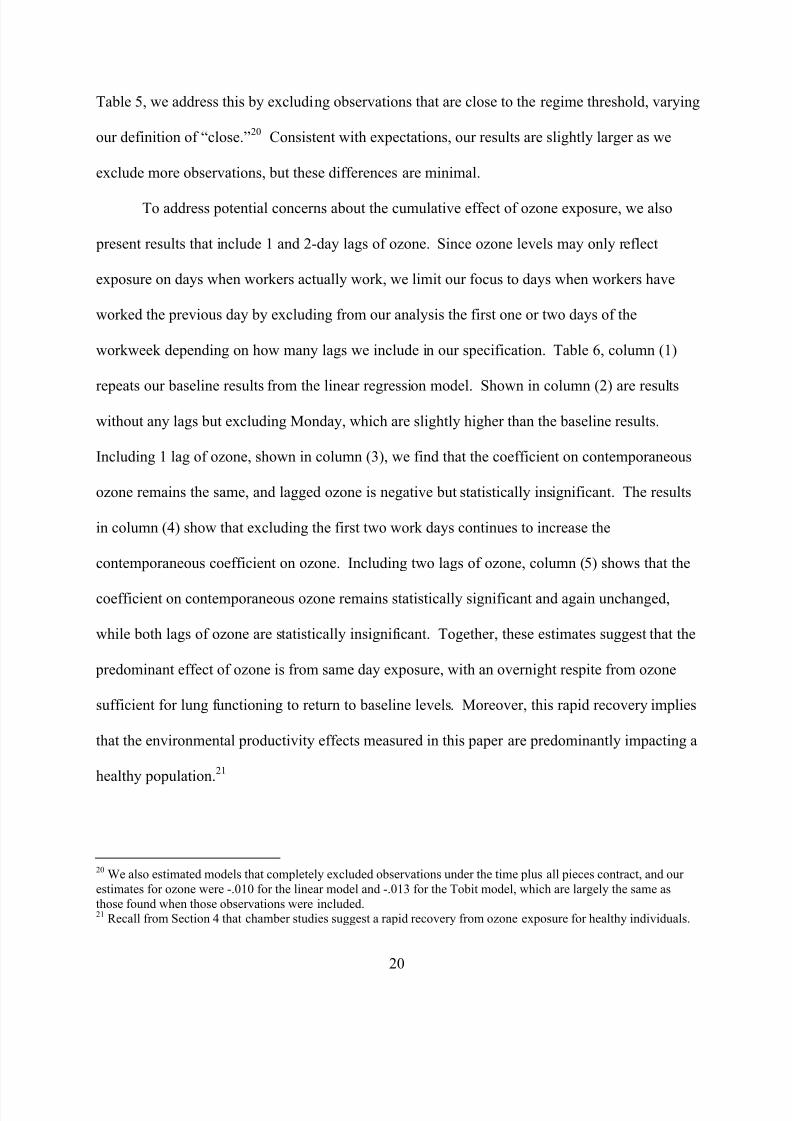
862019 Pllution and Working Effects
httpslidepdfcomreaderfullpllution-and-working-effects 2236
6 Conclusion
In this paper we merge a unique dataset on individual-level daily harvest rates for
agricultural workers with data on environmental conditions to assess the impact of ozone
pollution on worker productivity We find that a 10 ppb change in average ozone exposure
results in a significant and robust 42 percent change in agricultural worker productivity Despite
the applicability of minimum wages and the incentive to shirk we find little evidence of
differential effects depending on whether or not the minimum wage binds Importantly this
environmental productivity effect suggests that common characterizations of environmental
protection as purely a tax on producers and consumers to be weighed against the consumption
benefits associated with improved environmental quality may be misguided Environmental
protection can also be viewed as an investment in human capital and its contribution to firm
productivity and economic growth should be incorporated in the calculus of policy makers
Our results also speak to the ongoing debates on ozone policy Ozone pollution
continues to be a pervasive environmental issue throughout much of the world Debates over the
optimal level of ozone have ensued for many years and current efforts to strengthen these
standards remain contentious Defining regulatory thresholds depends in part on the benefits
associated with avoided exposure which has traditionally been estimated through a focus on
high-visibility health effects such as hospitalizations The labor productivity impacts measured
in this paper help make these benefits calculations more complete Our results indicate that
ozone even at levels below current air quality standards in most of the world has significant
negative impacts on worker productivity suggesting that the strengthening of regulations on
ozone pollution would yield additional benefits
21
862019 Pllution and Working Effects
httpslidepdfcomreaderfullpllution-and-working-effects 2336
These impacts of ozone on agricultural workers are also important in their own right A
back-of-the envelope calculation that applies the environmental productivity effect estimated in
the Central Valley of California to the whole of the US suggests that a 10 ppb reduction in the
ozone standard would translate into an annual cost savings of approximately $11 billion in labor
expenditure22
In the developing world where national incomes depend more heavily on
agriculture these productivity effects are likely to have a much larger impact on the economy
These impacts may be especially large in countries like India China and Mexico where rapid
industrial growth and automobile penetration contribute precursor chemicals that contribute to
substantially higher levels of ozone pollution
While the impacts of ozone on agricultural productivity are large the generalizability of
these findings to other pollutants and industries is unclear Agricultural workers face
considerably higher levels of exposure to pollution than individuals who work indoors That
said roughly 118 percent of the US labor force works in an industry with regular exposure to
outdoor conditions and this figure is much higher for middle- and lower-income countries (Graff
Zivin and Neidell 2010) Moreover many forms of outdoor pollution diminish indoor air
quality as well For example indoor penetration of fine particulate matter ranges from 38-94
for typical residential homes in the US (Abt et al 2000) Examining the generalizability of the
environmental productivity effect estimated in this paper to other pollutants and industries
represents a fruitful area for future research
22 Total labor expenditure in US agriculture was approximately $265B in 2007 (USDA 2009)
22
862019 Pllution and Working Effects
httpslidepdfcomreaderfullpllution-and-working-effects 2436
References
Abt Eileen Helen H Suh Paul Catalano and Petros Koutrakis (2000) ldquoRelative Contributionof Outdoor and Indoor Particle Sources to Indoor Concentrationsrdquo Environmental Science and Technology 34 (17) pp 3579ndash3587
Auffhammer Maximilian and Ryan Kellogg (2011) ldquoClearing the Air The Effects of GasolineContent Regulation on Air Qualityrdquo American Economic Review forthcoming
Bandiera Oriana Iwan Barankay and Imran Rasul (2005) ldquoSocial Preferences and theResponse to Incentives Evidence from Personnel Datardquo Quarterly Journal of Economics
120(3) 917-962
Bandiera Oriana Iwan Barankay and Imran Rasul (2010) ldquoSocial Incentives in theWorkplacerdquo Review of Economic Studies 77(2) 417-458
Banzhaf H Spencer and Randall Walsh (2008) ldquoDo People Vote with Their Feet AnEmpirical Test of Tieboutrdquo American Economic Review 98(3) 843ndash63
Bell Michelle Aidan McDermott Scott Zeger Jonathan Samet Francesca Dominici (2004)ldquoOzone and Short-term Mortality in 95 US Urban Communities 1987-2000rdquo Journal of the American Medical Association 292 (19)
Blanchard Charles and Shelley Tanenbaum (2003) ldquoDifferences between Weekday andWeekend Air Pollutant Levels in Southern Californiardquo Journal of the Air and Waste
Management Association 53(7)
Brauer M and JR Brook (1995) ldquoPersonal and Fixed-Site Ozone Measurementswith a Passive Samplerrdquo Journal of the Air and Waste Management Association 45 (7) 529-537
Brauer M J Blair and S Vedal (1996) ldquoEffect of ambient ozone exposure on lung function infarm workersrdquo Am J Respir Crit Care Med 154(4) 981-987
Carson Richard Phoebe Koundouri and Ceacuteline Nauges (2010) ldquoArsenic Mitigation inBangladesh A Household Labor Market Approachrdquo American Journal of Agricultural Economics 92
Chan Chang-Chuan and Tsung-Huan Wu (2005) ldquoEffects of Ambient Ozone Exposure on MailCarriers Peak Expiratory Flow Ratesrdquo Environmental Health Perspectives 113(6) 735-738
Chay Kenneth and Michael Greenstone (2003) ldquoThe Impact of Air Pollution on InfantMortality Evidence from Geographic Variation in Pollution Shocks Induced by a RecessionrdquoQuarterly Journal of Economics 118(3) 1121-1167
23
862019 Pllution and Working Effects
httpslidepdfcomreaderfullpllution-and-working-effects 2536
Chay Kenneth and Michael Greenstone (2005) ldquoDoes Air Quality Matter Evidence from theHousing Marketrdquo Journal of Political Economy 113 376ndash424
Chernozhukov Victor and Han Hong (2002) ldquoThree-step censored quantile regression andextramarital affairsrdquo Journal of the American Statistical Association 97(459) 872-882
Currie Janet and Matthew Neidell (2005) ldquoAir Pollution and Infant Health What Can We Learnfrom Californias Recent Experiencerdquo Quarterly Journal of Economics 120(3) 1003-1030
Dockery Douglas W C Arden Pope Xiping Xu John D Spengler James H Ware Martha EFay Benjamin G Ferris and Frank E Speizer (1993) ldquoAn association between air pollution andmortality in six US citiesrdquo The New England Journal of Medicine 3291753-1759
Environmental Protection Agency (2010) ldquoNational Ambient Air Quality Standards for Ozone(Proposed Rule)rdquo Federal Register 7511 (January 19 2010) p 2938-3052
Folinsbee L J Hazucha M J (2000) ldquoTime course of response to ozone exposure in healthyadult femalesrdquo Inhalation Toxicol 12 151-167
Folinsbee L J Horvath S M (1986) ldquoPersistence of the acute effects of ozone exposurerdquo Aviat Space Environ Med 57 1136-1143
Gong H Jr Bradley P W Simmons M S Tashkin D P (1986) ldquoImpaired exercise performance and pulmonary function in elite cyclists during low-level ozone exposure in a hotenvironmentrdquo Am Rev Respir Dis 134 726-733
Graff Zivin Joshua and Matthew Neidell (2010) ldquoTemperature and the allocation of timeImplications for climate changerdquo NBER working paper 15717
Hanna Rema and Paulina Oliva (2011) ldquoThe Effect of Pollution on Labor Supply Evidencefrom a Natural Experiment in Mexico Cityrdquo Mimeo
Hazucha M J LJ Folinsbee and PA Bromberg (2003) ldquoDistribution and reproducibility of spirometric response to ozone by gender and agerdquo J Appl Physiol 95 1917-1925
Hausman Jerry Bart Ostro and David Wise (1984) ldquoAir Pollution and Lost Workrdquo NBER Working Paper No 1263
Kulle T J Sauder L R Hebel J R Chatham M D (1985) rdquoOzone response relationshipsin healthy nonsmokersrdquo Am Rev Respir Dis 132 36-41
Lazear Edward (2000) ldquoPerformance pay and productivityrdquo American Economic Review 90(5)1346-1361
24
862019 Pllution and Working Effects
httpslidepdfcomreaderfullpllution-and-working-effects 2636
Manning WJ (2003) ldquoAssessing plant responses to ambient ozone Growth of ozone-sensitiveloblolly pine seedlings treated with ethylenediurea (EDU) and sodium erythorbate (NaE)rdquo Environ Pollut 126(1) 73-81
McDonnell W F Horstman D H Hazucha M J Seal E Jr Haak E D Salaam S A
House D E (1983) ldquoPulmonary effects of ozone exposure during exercise dose-responsecharacteristicsrdquo J Appl Physiol Respir Environ Exercise Physiol 54 1345-1352
Neidell Matthew (2009) ldquoInformation Avoidance Behavior and Health The Effect of Ozoneon Asthma Hospitalizationsrdquo Journal of Human Resources 44(2)
ONeill MS Ramirez-Aguilar M Meneses-Gonzalez F Hernaacutendez-Avila M Geyh AS Sienra-Monge JJ Romieu I (2003) ldquoOzone exposure among Mexico City outdoor workersrdquo J Air
Waste Manag Assoc 53(3) 339-46
Ostro Bart (1983) ldquoThe Effects of Air Pollution on Work Lost and Morbidity Journal of
Environmental Economics and Management 10(4) 371-382
Paarsch Harry J and Bruce Shearer (1999) ldquoThe Response of Worker Effort to Piece RatesEvidence from the British Columbia Tree-Planting Industry Journal of Human Resources 34643-667
Paarsch Harry J and Bruce Shearer (2000) ldquoPiece Rates Fixed Wages and Incentive EffectsStatistical Evidence from Payroll Records International Economic Review 40 59-92
Pope CA III Burnett RT Thun MJ Calle EE Krewski D Ito K Thurston GD (2002) ldquoLungCancer Cardiopulmonary Mortality and Long-term Exposure to Fine Particulate Air Pollutionrdquo Journal of the American Medical Association 2871132-1141
Shapiro Carl and Joseph Stiglitz (1984) ldquoEquilibrium unemployment as a worker disciplinedevicerdquo American Economic Review 74(3)
Shi Lan (2010) ldquoIncentive Effect of Piece Rate Contracts Evidence from Two Small FieldExperimentsrdquo The BE Journal of Economic Analysis amp Policy 10(1) (Topics)
Sillman Sanford (1999) ldquoThe Relation Between Ozone NOx and Hydrocarbons in Urban andPolluted Rural Environmentsrdquo Atmospheric Environment 33 1821-1845
Tepper J S Costa D L Lehmann J R Weber M F Hatch G E (1989) ldquoUnattenuatedstructural and biochemical alterations in the rat lung during functional adaptation to ozonerdquo Am
Rev Respir Dis 140 493-501
USDA (2009) 2007 Census of Agriculture (AC-07-A-5) National Agricultural StatisticsService Washington DC
25
862019 Pllution and Working Effects
httpslidepdfcomreaderfullpllution-and-working-effects 2736
Figure 1 Standardized average hourly pieces collected by crop and for all crops
Notes We standardize average hourly productivity by subtracting the minimum number of pieces per hour requiredto reach the piece rate regime and dividing by the standard deviation of productivity for each crop The vertical linereflects the regime threshold for crossing from the minimum wage to the piece rate regime
0
2
4
6
0
2
4
6
-5 0 5 -5 0 5
Crop 1 (time+all pieces) Crop 2 (time+pieces $03p)
Crop 3 (time+pieces $1p) Total
D e n s i t y
26
862019 Pllution and Working Effects
httpslidepdfcomreaderfullpllution-and-working-effects 2836
Figure 2 Variation in productivity by worker all crops
0
1
2
3
4
5
D e n s i t y
-4 -2 0 2
27
862019 Pllution and Working Effects
httpslidepdfcomreaderfullpllution-and-working-effects 2936
Figure 3 Variation in productivity by day all crops
0
2
4
6
D e n s i t y
-3 -2 -1 0 1 2
28
862019 Pllution and Working Effects
httpslidepdfcomreaderfullpllution-and-working-effects 3036
Figure 4 Average demeaned daily ozone and temperature in 2010
-40
-30
-20
-10
0
10
20
30
40
50
512010 612010 712010 812010 912010 1012010
d e m e a n e d v a l u e
ozone temperature harves t day
29
862019 Pllution and Working Effects
httpslidepdfcomreaderfullpllution-and-working-effects 3136
Table 1 Summary statistics
A Productivity variables (n=36215)Observations mean SD SD within
worker SD between
workers
1 Minimum wage regimeHourly pieces (crop 1) 11753 203 057 044 047Hourly pieces (crop 2) 4114 308 077 065 069Hourly pieces (crop 3) 5920 229 048 031 044hours worked 21787 763 129 076 1202 Piece rate regimeHourly pieces (crop 1) 3675 342 040 030 032Hourly pieces (crop 2) 5512 492 085 061 064Hourly pieces (crop 3) 5241 388 082 050 066hours worked 14428 734 152 096 135
B Environmental variables (n=155)mean SD min maxozone (ppb) 4777 1324 1050 8600temperature (F) 7815 852 5630 9698atmospheric pressure (mb) 100155 648 98886 101259resultant wind speed (mph) 274 053 161 460solar radiation (Wm2) 83733 17407 18700 108333relative humidity () 4533 1004 2790 9350 precipitation (mm) 240 505 000 3548
C Sample
total of dates 155total of employees 1664mean of days with farm 20
Notes SD Standard deviation Crop 1 is time plus all pieces with a piece rate of $05piece and minimum pieces per hour of 3 Crop 2 is time plus pieces with a piece rate of $03piece and minimum pieces per hour of 4 Crop 3 istime plus pieces with a piece rate of $1piece and minimum pieces per hour of 3
30
862019 Pllution and Working Effects
httpslidepdfcomreaderfullpllution-and-working-effects 3236
Table 2 Regression results of the effect of ozone on avoidance behavior
1 2 3 4
extensive margin probability(work)
intensive margin hours worked
ozone (ppb) -00017 -00018 00014 00014[00020] [00021] [00123] [00125]worker fixed effect N Y N YObservations 39223 39223 36215 36215R-squared 011 016 024 027Standard errors clustered on date and worker in brackets significant at 10 significant at 5 significantat 1 All regressions include controls for temperature (quadratic) air pressure wind speed solar radiation relativehumidity precipitation day of week dummies monthyear dummies and piece rate contract type dummies Allenvironmental variables are the mean of hourly values from 6am-3pm
31
862019 Pllution and Working Effects
httpslidepdfcomreaderfullpllution-and-working-effects 3336
Table 3 Main regression results of the effect of ozone on productivity
1 2 3 4
ozone (ppb) -00116 -00123 -00092 -00124[00043] [00052] [00055] [00058]
model linear Tobit median censoredmedianObservations 36215 36215 36215 36215(Psuedo) R2 031 010 019 024Standard errors clustered on date and worker in brackets significant at 10 significant at 5 significantat 1 The dependent variable is standardized hourly pieces collected All regressions include controls for temperature (quadratic) air pressure wind speed solar radiation relative humidity precipitation day of week dummies monthyear dummies and piece rate contract type dummies All environmental variables are the mean of hourly values from 6am-3pm Bootstrapped standard errors for both median regressions were obtained using 50replications
32
862019 Pllution and Working Effects
httpslidepdfcomreaderfullpllution-and-working-effects 3436
Table 4 Separation rates by productivity decile
1 2 3 4
A Unadjusted productivity B Productivity adjusted for tenure
productivitydecile separation rate tenure (days) separation rate tenure (days)
1 0065 1244 0061 17992 0060 1555 0063 19203 0047 1658 0055 18474 0053 1896 0047 19475 0034 1864 0047 21566 0042 2128 0039 22137 0044 2109 0038 19248 0032 2227 0029 18729 0025 2324 0024 1941
10 0025 2431 0023 1817This table shows daily mean separation rates and tenure by productivity decile
33
862019 Pllution and Working Effects
httpslidepdfcomreaderfullpllution-and-working-effects 3536
Table 5 Sensitivity of regression results of the effect of ozone on productivity
1 2 3 4 5 6
A Linear model
ozone (ppb) -00116 -00097 -00125 -00111 -00129 -00136
[00043] [00041] [00045] [00050] [00048] [00052]R-squared 031 053 031 033 032 033
B Tobit model
ozone (ppb) -00123 -00105 -00121 -00130 -00146 -00154[00052] [00049] [00053] [00059] [00057] [00064]
Pseudo R-squared
010 031 010 011 012 013
model baseline worker fixed
effect
includemin and
max of temp(quadratic)and solar
rad
includemin and
max of temp(indicators)and solar
rad
excludeobs 1 SD
of regimethreshold
excludeobs 2 SD
of regimethreshold
Observations 36215 36215 36215 36215 32415 30239Standard errors clustered on date and worker in brackets significant at 10 significant at 5 significantat 1 The dependent variable is standardized hourly pieces collected All regressions include controls for temperature (quadratic except column 4 which includes indicator variables for every 5 degrees F) air pressurewind speed solar radiation relative humidity precipitation day of week dummies monthyear dummies and piecerate contract type dummies All environmental variables are based on hourly values from 6am-3pm
34
862019 Pllution and Working Effects
httpslidepdfcomreaderfullpllution-and-working-effects 3636
Table 6 Regression results of the effect of lagged ozone on productivity
1 2 3 4 5
A Linear model
ozone (ppb) -0011 -0013 -0013 -0016 -0015
[0004] [0005] [0005] [0005] [0005]1 lag ozone (ppb) -0004 -0006[0004] [0006]
2 lag ozone (ppb) 0003[0005]
R-squared 031 032 032 032 032
B Tobit model
ozone (ppb) -0012 -0013 -0012 -0016 -0014[0005] [0006] [0006] [0006] [0006]
1 lag ozone (ppb) -0003 -0003
[0005] [0007]2 lag ozone (ppb) 0001[0005]
Pseudo R-squared 010 010 010 010 010
Day(s) of week excluded
none Monday Monday Monday ampTuesday
Monday ampTuesday
Observations 35465 25456 25456 17498 17498Standard errors clustered on date and worker in brackets significant at 10 significant at 5 significantat 1 The dependent variable is standardized hourly pieces collected All regressions control for temperature(quadratic) air pressure wind speed solar radiation relative humidity precipitation day of week dummiesmonthyear dummies and piece rate contract type dummies All environmental variables are the mean of hourly
values from 6am-3pm
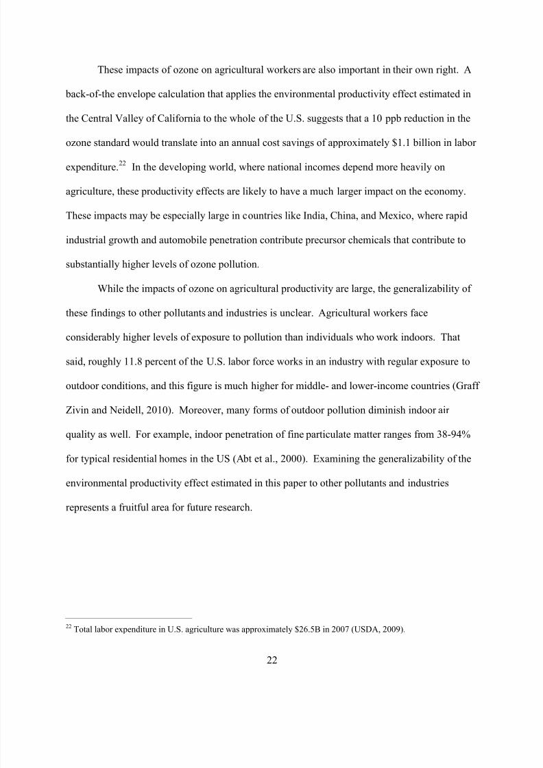
862019 Pllution and Working Effects
httpslidepdfcomreaderfullpllution-and-working-effects 2636
Manning WJ (2003) ldquoAssessing plant responses to ambient ozone Growth of ozone-sensitiveloblolly pine seedlings treated with ethylenediurea (EDU) and sodium erythorbate (NaE)rdquo Environ Pollut 126(1) 73-81
McDonnell W F Horstman D H Hazucha M J Seal E Jr Haak E D Salaam S A
House D E (1983) ldquoPulmonary effects of ozone exposure during exercise dose-responsecharacteristicsrdquo J Appl Physiol Respir Environ Exercise Physiol 54 1345-1352
Neidell Matthew (2009) ldquoInformation Avoidance Behavior and Health The Effect of Ozoneon Asthma Hospitalizationsrdquo Journal of Human Resources 44(2)
ONeill MS Ramirez-Aguilar M Meneses-Gonzalez F Hernaacutendez-Avila M Geyh AS Sienra-Monge JJ Romieu I (2003) ldquoOzone exposure among Mexico City outdoor workersrdquo J Air
Waste Manag Assoc 53(3) 339-46
Ostro Bart (1983) ldquoThe Effects of Air Pollution on Work Lost and Morbidity Journal of
Environmental Economics and Management 10(4) 371-382
Paarsch Harry J and Bruce Shearer (1999) ldquoThe Response of Worker Effort to Piece RatesEvidence from the British Columbia Tree-Planting Industry Journal of Human Resources 34643-667
Paarsch Harry J and Bruce Shearer (2000) ldquoPiece Rates Fixed Wages and Incentive EffectsStatistical Evidence from Payroll Records International Economic Review 40 59-92
Pope CA III Burnett RT Thun MJ Calle EE Krewski D Ito K Thurston GD (2002) ldquoLungCancer Cardiopulmonary Mortality and Long-term Exposure to Fine Particulate Air Pollutionrdquo Journal of the American Medical Association 2871132-1141
Shapiro Carl and Joseph Stiglitz (1984) ldquoEquilibrium unemployment as a worker disciplinedevicerdquo American Economic Review 74(3)
Shi Lan (2010) ldquoIncentive Effect of Piece Rate Contracts Evidence from Two Small FieldExperimentsrdquo The BE Journal of Economic Analysis amp Policy 10(1) (Topics)
Sillman Sanford (1999) ldquoThe Relation Between Ozone NOx and Hydrocarbons in Urban andPolluted Rural Environmentsrdquo Atmospheric Environment 33 1821-1845
Tepper J S Costa D L Lehmann J R Weber M F Hatch G E (1989) ldquoUnattenuatedstructural and biochemical alterations in the rat lung during functional adaptation to ozonerdquo Am
Rev Respir Dis 140 493-501
USDA (2009) 2007 Census of Agriculture (AC-07-A-5) National Agricultural StatisticsService Washington DC
25
862019 Pllution and Working Effects
httpslidepdfcomreaderfullpllution-and-working-effects 2736
Figure 1 Standardized average hourly pieces collected by crop and for all crops
Notes We standardize average hourly productivity by subtracting the minimum number of pieces per hour requiredto reach the piece rate regime and dividing by the standard deviation of productivity for each crop The vertical linereflects the regime threshold for crossing from the minimum wage to the piece rate regime
0
2
4
6
0
2
4
6
-5 0 5 -5 0 5
Crop 1 (time+all pieces) Crop 2 (time+pieces $03p)
Crop 3 (time+pieces $1p) Total
D e n s i t y
26
862019 Pllution and Working Effects
httpslidepdfcomreaderfullpllution-and-working-effects 2836
Figure 2 Variation in productivity by worker all crops
0
1
2
3
4
5
D e n s i t y
-4 -2 0 2
27
862019 Pllution and Working Effects
httpslidepdfcomreaderfullpllution-and-working-effects 2936
Figure 3 Variation in productivity by day all crops
0
2
4
6
D e n s i t y
-3 -2 -1 0 1 2
28
862019 Pllution and Working Effects
httpslidepdfcomreaderfullpllution-and-working-effects 3036
Figure 4 Average demeaned daily ozone and temperature in 2010
-40
-30
-20
-10
0
10
20
30
40
50
512010 612010 712010 812010 912010 1012010
d e m e a n e d v a l u e
ozone temperature harves t day
29
862019 Pllution and Working Effects
httpslidepdfcomreaderfullpllution-and-working-effects 3136
Table 1 Summary statistics
A Productivity variables (n=36215)Observations mean SD SD within
worker SD between
workers
1 Minimum wage regimeHourly pieces (crop 1) 11753 203 057 044 047Hourly pieces (crop 2) 4114 308 077 065 069Hourly pieces (crop 3) 5920 229 048 031 044hours worked 21787 763 129 076 1202 Piece rate regimeHourly pieces (crop 1) 3675 342 040 030 032Hourly pieces (crop 2) 5512 492 085 061 064Hourly pieces (crop 3) 5241 388 082 050 066hours worked 14428 734 152 096 135
B Environmental variables (n=155)mean SD min maxozone (ppb) 4777 1324 1050 8600temperature (F) 7815 852 5630 9698atmospheric pressure (mb) 100155 648 98886 101259resultant wind speed (mph) 274 053 161 460solar radiation (Wm2) 83733 17407 18700 108333relative humidity () 4533 1004 2790 9350 precipitation (mm) 240 505 000 3548
C Sample
total of dates 155total of employees 1664mean of days with farm 20
Notes SD Standard deviation Crop 1 is time plus all pieces with a piece rate of $05piece and minimum pieces per hour of 3 Crop 2 is time plus pieces with a piece rate of $03piece and minimum pieces per hour of 4 Crop 3 istime plus pieces with a piece rate of $1piece and minimum pieces per hour of 3
30
862019 Pllution and Working Effects
httpslidepdfcomreaderfullpllution-and-working-effects 3236
Table 2 Regression results of the effect of ozone on avoidance behavior
1 2 3 4
extensive margin probability(work)
intensive margin hours worked
ozone (ppb) -00017 -00018 00014 00014[00020] [00021] [00123] [00125]worker fixed effect N Y N YObservations 39223 39223 36215 36215R-squared 011 016 024 027Standard errors clustered on date and worker in brackets significant at 10 significant at 5 significantat 1 All regressions include controls for temperature (quadratic) air pressure wind speed solar radiation relativehumidity precipitation day of week dummies monthyear dummies and piece rate contract type dummies Allenvironmental variables are the mean of hourly values from 6am-3pm
31
862019 Pllution and Working Effects
httpslidepdfcomreaderfullpllution-and-working-effects 3336
Table 3 Main regression results of the effect of ozone on productivity
1 2 3 4
ozone (ppb) -00116 -00123 -00092 -00124[00043] [00052] [00055] [00058]
model linear Tobit median censoredmedianObservations 36215 36215 36215 36215(Psuedo) R2 031 010 019 024Standard errors clustered on date and worker in brackets significant at 10 significant at 5 significantat 1 The dependent variable is standardized hourly pieces collected All regressions include controls for temperature (quadratic) air pressure wind speed solar radiation relative humidity precipitation day of week dummies monthyear dummies and piece rate contract type dummies All environmental variables are the mean of hourly values from 6am-3pm Bootstrapped standard errors for both median regressions were obtained using 50replications
32
862019 Pllution and Working Effects
httpslidepdfcomreaderfullpllution-and-working-effects 3436
Table 4 Separation rates by productivity decile
1 2 3 4
A Unadjusted productivity B Productivity adjusted for tenure
productivitydecile separation rate tenure (days) separation rate tenure (days)
1 0065 1244 0061 17992 0060 1555 0063 19203 0047 1658 0055 18474 0053 1896 0047 19475 0034 1864 0047 21566 0042 2128 0039 22137 0044 2109 0038 19248 0032 2227 0029 18729 0025 2324 0024 1941
10 0025 2431 0023 1817This table shows daily mean separation rates and tenure by productivity decile
33
862019 Pllution and Working Effects
httpslidepdfcomreaderfullpllution-and-working-effects 3536
Table 5 Sensitivity of regression results of the effect of ozone on productivity
1 2 3 4 5 6
A Linear model
ozone (ppb) -00116 -00097 -00125 -00111 -00129 -00136
[00043] [00041] [00045] [00050] [00048] [00052]R-squared 031 053 031 033 032 033
B Tobit model
ozone (ppb) -00123 -00105 -00121 -00130 -00146 -00154[00052] [00049] [00053] [00059] [00057] [00064]
Pseudo R-squared
010 031 010 011 012 013
model baseline worker fixed
effect
includemin and
max of temp(quadratic)and solar
rad
includemin and
max of temp(indicators)and solar
rad
excludeobs 1 SD
of regimethreshold
excludeobs 2 SD
of regimethreshold
Observations 36215 36215 36215 36215 32415 30239Standard errors clustered on date and worker in brackets significant at 10 significant at 5 significantat 1 The dependent variable is standardized hourly pieces collected All regressions include controls for temperature (quadratic except column 4 which includes indicator variables for every 5 degrees F) air pressurewind speed solar radiation relative humidity precipitation day of week dummies monthyear dummies and piecerate contract type dummies All environmental variables are based on hourly values from 6am-3pm
34
862019 Pllution and Working Effects
httpslidepdfcomreaderfullpllution-and-working-effects 3636
Table 6 Regression results of the effect of lagged ozone on productivity
1 2 3 4 5
A Linear model
ozone (ppb) -0011 -0013 -0013 -0016 -0015
[0004] [0005] [0005] [0005] [0005]1 lag ozone (ppb) -0004 -0006[0004] [0006]
2 lag ozone (ppb) 0003[0005]
R-squared 031 032 032 032 032
B Tobit model
ozone (ppb) -0012 -0013 -0012 -0016 -0014[0005] [0006] [0006] [0006] [0006]
1 lag ozone (ppb) -0003 -0003
[0005] [0007]2 lag ozone (ppb) 0001[0005]
Pseudo R-squared 010 010 010 010 010
Day(s) of week excluded
none Monday Monday Monday ampTuesday
Monday ampTuesday
Observations 35465 25456 25456 17498 17498Standard errors clustered on date and worker in brackets significant at 10 significant at 5 significantat 1 The dependent variable is standardized hourly pieces collected All regressions control for temperature(quadratic) air pressure wind speed solar radiation relative humidity precipitation day of week dummiesmonthyear dummies and piece rate contract type dummies All environmental variables are the mean of hourly
values from 6am-3pm
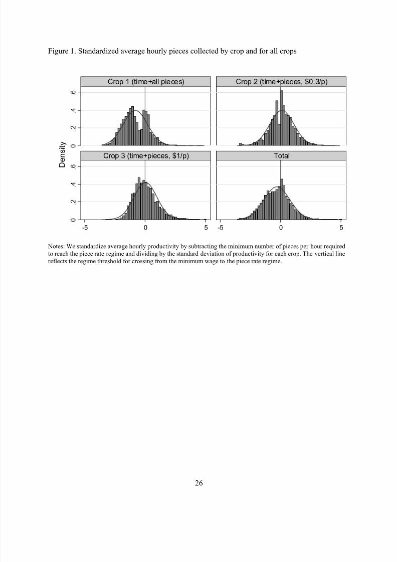
862019 Pllution and Working Effects
httpslidepdfcomreaderfullpllution-and-working-effects 2736
Figure 1 Standardized average hourly pieces collected by crop and for all crops
Notes We standardize average hourly productivity by subtracting the minimum number of pieces per hour requiredto reach the piece rate regime and dividing by the standard deviation of productivity for each crop The vertical linereflects the regime threshold for crossing from the minimum wage to the piece rate regime
0
2
4
6
0
2
4
6
-5 0 5 -5 0 5
Crop 1 (time+all pieces) Crop 2 (time+pieces $03p)
Crop 3 (time+pieces $1p) Total
D e n s i t y
26
862019 Pllution and Working Effects
httpslidepdfcomreaderfullpllution-and-working-effects 2836
Figure 2 Variation in productivity by worker all crops
0
1
2
3
4
5
D e n s i t y
-4 -2 0 2
27
862019 Pllution and Working Effects
httpslidepdfcomreaderfullpllution-and-working-effects 2936
Figure 3 Variation in productivity by day all crops
0
2
4
6
D e n s i t y
-3 -2 -1 0 1 2
28
862019 Pllution and Working Effects
httpslidepdfcomreaderfullpllution-and-working-effects 3036
Figure 4 Average demeaned daily ozone and temperature in 2010
-40
-30
-20
-10
0
10
20
30
40
50
512010 612010 712010 812010 912010 1012010
d e m e a n e d v a l u e
ozone temperature harves t day
29
862019 Pllution and Working Effects
httpslidepdfcomreaderfullpllution-and-working-effects 3136
Table 1 Summary statistics
A Productivity variables (n=36215)Observations mean SD SD within
worker SD between
workers
1 Minimum wage regimeHourly pieces (crop 1) 11753 203 057 044 047Hourly pieces (crop 2) 4114 308 077 065 069Hourly pieces (crop 3) 5920 229 048 031 044hours worked 21787 763 129 076 1202 Piece rate regimeHourly pieces (crop 1) 3675 342 040 030 032Hourly pieces (crop 2) 5512 492 085 061 064Hourly pieces (crop 3) 5241 388 082 050 066hours worked 14428 734 152 096 135
B Environmental variables (n=155)mean SD min maxozone (ppb) 4777 1324 1050 8600temperature (F) 7815 852 5630 9698atmospheric pressure (mb) 100155 648 98886 101259resultant wind speed (mph) 274 053 161 460solar radiation (Wm2) 83733 17407 18700 108333relative humidity () 4533 1004 2790 9350 precipitation (mm) 240 505 000 3548
C Sample
total of dates 155total of employees 1664mean of days with farm 20
Notes SD Standard deviation Crop 1 is time plus all pieces with a piece rate of $05piece and minimum pieces per hour of 3 Crop 2 is time plus pieces with a piece rate of $03piece and minimum pieces per hour of 4 Crop 3 istime plus pieces with a piece rate of $1piece and minimum pieces per hour of 3
30
862019 Pllution and Working Effects
httpslidepdfcomreaderfullpllution-and-working-effects 3236
Table 2 Regression results of the effect of ozone on avoidance behavior
1 2 3 4
extensive margin probability(work)
intensive margin hours worked
ozone (ppb) -00017 -00018 00014 00014[00020] [00021] [00123] [00125]worker fixed effect N Y N YObservations 39223 39223 36215 36215R-squared 011 016 024 027Standard errors clustered on date and worker in brackets significant at 10 significant at 5 significantat 1 All regressions include controls for temperature (quadratic) air pressure wind speed solar radiation relativehumidity precipitation day of week dummies monthyear dummies and piece rate contract type dummies Allenvironmental variables are the mean of hourly values from 6am-3pm
31
862019 Pllution and Working Effects
httpslidepdfcomreaderfullpllution-and-working-effects 3336
Table 3 Main regression results of the effect of ozone on productivity
1 2 3 4
ozone (ppb) -00116 -00123 -00092 -00124[00043] [00052] [00055] [00058]
model linear Tobit median censoredmedianObservations 36215 36215 36215 36215(Psuedo) R2 031 010 019 024Standard errors clustered on date and worker in brackets significant at 10 significant at 5 significantat 1 The dependent variable is standardized hourly pieces collected All regressions include controls for temperature (quadratic) air pressure wind speed solar radiation relative humidity precipitation day of week dummies monthyear dummies and piece rate contract type dummies All environmental variables are the mean of hourly values from 6am-3pm Bootstrapped standard errors for both median regressions were obtained using 50replications
32
862019 Pllution and Working Effects
httpslidepdfcomreaderfullpllution-and-working-effects 3436
Table 4 Separation rates by productivity decile
1 2 3 4
A Unadjusted productivity B Productivity adjusted for tenure
productivitydecile separation rate tenure (days) separation rate tenure (days)
1 0065 1244 0061 17992 0060 1555 0063 19203 0047 1658 0055 18474 0053 1896 0047 19475 0034 1864 0047 21566 0042 2128 0039 22137 0044 2109 0038 19248 0032 2227 0029 18729 0025 2324 0024 1941
10 0025 2431 0023 1817This table shows daily mean separation rates and tenure by productivity decile
33
862019 Pllution and Working Effects
httpslidepdfcomreaderfullpllution-and-working-effects 3536
Table 5 Sensitivity of regression results of the effect of ozone on productivity
1 2 3 4 5 6
A Linear model
ozone (ppb) -00116 -00097 -00125 -00111 -00129 -00136
[00043] [00041] [00045] [00050] [00048] [00052]R-squared 031 053 031 033 032 033
B Tobit model
ozone (ppb) -00123 -00105 -00121 -00130 -00146 -00154[00052] [00049] [00053] [00059] [00057] [00064]
Pseudo R-squared
010 031 010 011 012 013
model baseline worker fixed
effect
includemin and
max of temp(quadratic)and solar
rad
includemin and
max of temp(indicators)and solar
rad
excludeobs 1 SD
of regimethreshold
excludeobs 2 SD
of regimethreshold
Observations 36215 36215 36215 36215 32415 30239Standard errors clustered on date and worker in brackets significant at 10 significant at 5 significantat 1 The dependent variable is standardized hourly pieces collected All regressions include controls for temperature (quadratic except column 4 which includes indicator variables for every 5 degrees F) air pressurewind speed solar radiation relative humidity precipitation day of week dummies monthyear dummies and piecerate contract type dummies All environmental variables are based on hourly values from 6am-3pm
34
862019 Pllution and Working Effects
httpslidepdfcomreaderfullpllution-and-working-effects 3636
Table 6 Regression results of the effect of lagged ozone on productivity
1 2 3 4 5
A Linear model
ozone (ppb) -0011 -0013 -0013 -0016 -0015
[0004] [0005] [0005] [0005] [0005]1 lag ozone (ppb) -0004 -0006[0004] [0006]
2 lag ozone (ppb) 0003[0005]
R-squared 031 032 032 032 032
B Tobit model
ozone (ppb) -0012 -0013 -0012 -0016 -0014[0005] [0006] [0006] [0006] [0006]
1 lag ozone (ppb) -0003 -0003
[0005] [0007]2 lag ozone (ppb) 0001[0005]
Pseudo R-squared 010 010 010 010 010
Day(s) of week excluded
none Monday Monday Monday ampTuesday
Monday ampTuesday
Observations 35465 25456 25456 17498 17498Standard errors clustered on date and worker in brackets significant at 10 significant at 5 significantat 1 The dependent variable is standardized hourly pieces collected All regressions control for temperature(quadratic) air pressure wind speed solar radiation relative humidity precipitation day of week dummiesmonthyear dummies and piece rate contract type dummies All environmental variables are the mean of hourly
values from 6am-3pm
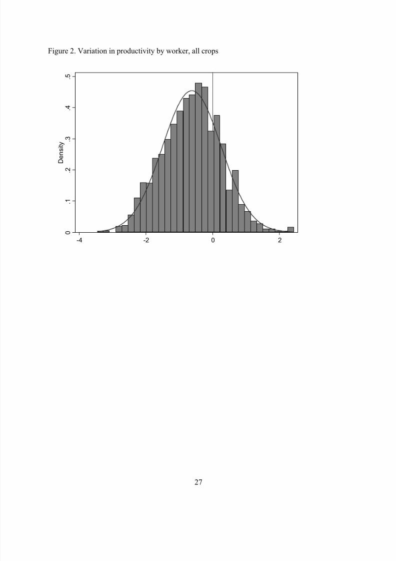
862019 Pllution and Working Effects
httpslidepdfcomreaderfullpllution-and-working-effects 3636
Table 6 Regression results of the effect of lagged ozone on productivity
1 2 3 4 5
A Linear model
ozone (ppb) -0011 -0013 -0013 -0016 -0015
[0004] [0005] [0005] [0005] [0005]1 lag ozone (ppb) -0004 -0006[0004] [0006]
2 lag ozone (ppb) 0003[0005]
R-squared 031 032 032 032 032
B Tobit model
ozone (ppb) -0012 -0013 -0012 -0016 -0014[0005] [0006] [0006] [0006] [0006]
1 lag ozone (ppb) -0003 -0003
[0005] [0007]2 lag ozone (ppb) 0001[0005]
Pseudo R-squared 010 010 010 010 010
Day(s) of week excluded
none Monday Monday Monday ampTuesday
Monday ampTuesday
Observations 35465 25456 25456 17498 17498Standard errors clustered on date and worker in brackets significant at 10 significant at 5 significantat 1 The dependent variable is standardized hourly pieces collected All regressions control for temperature(quadratic) air pressure wind speed solar radiation relative humidity precipitation day of week dummiesmonthyear dummies and piece rate contract type dummies All environmental variables are the mean of hourly
values from 6am-3pm