pls path modeling â€“ a software review - sfb 649 - humboldt

SFB 649 Discussion Paper 2006-084

PLS Path Modeling – A Software Review

Dirk Temme*

Henning Kreis* Lutz Hildebrandt*

* Institute of Marketing, Humboldt-Universität zu Berlin, Germany

This research was supported by the Deutsche Forschungsgemeinschaft through the SFB 649 "Economic Risk".

http://sfb649.wiwi.hu-berlin.de

ISSN 1860-5664

SFB 649, Humboldt-Universität zu Berlin Spandauer Straße 1, D-10178 Berlin

SFB

6

4 9

E

C O

N O

M I

C

R

I S

K

B

E R

L I

N

PLS Path Modeling – A Software Review1

Dirk Temme, Henning Kreis and Lutz Hildebrandt

Institute of Marketing, Humboldt University Berlin Spandauer Straße 1, 10099 Berlin

{temme, kreis, hildebr}@wiwi.hu-berlin.de

Abstract After years of stagnancy, PLS path modeling has recently attracted renewed interest from applied researchers in marketing. At the same time, the availability of software alternatives to Lohmöller’s LVPLS package has considerably increased (PLS-Graph, PLS-GUI, SPAD-PLS, SmartPLS). To help the user to make an informed decision, the existing programs are reviewed; their strengths and weaknesses are identified. Furthermore, analyzing simulated data reveals that the signs of weights/factor loadings and path coefficients can vary considerably across the different programs. Thus, applied researchers should treat the interpretation of their results with caution. Compared to programs for analysis of covariance structure models (LISREL approach), PLS path modeling software is on equal footing regarding ease of use, but clearly lags behind in terms of methodological capabilities. Keywords: PLS path modeling, Marketing, Formative indicators, Reflective indicators JEL-Codes: C31, C87, M31

1 Financial support by the Deutsche Forschungsgemeinschaft (DFG) through the SFB 649 “Economic Risk” is gratefully acknowledged.

PLS Path Modeling – A Software Review

Dirk Temme1, Henning Kreis2, and Lutz Hildebrandt3

1 Institute of Marketing, Humboldt University Berlin, Spandauer Str. 1, 10099Berlin, Germany, [email protected]

2 [email protected] [email protected]

1 Introduction

When it comes to modeling relationships between latent variables, mainly twodifferent methodological approaches can be distinguished: Covariance struc-ture analysis on the one hand and PLS path modeling (not to be confused withPLS regression) on the other. Although both methods emerged roughly at thesame time, their development took a rather diverse course. Since the intro-duction of the first LISREL version in the early 1970s, the software availablefor covariance structure analysis has experienced substantial progress withrespect to ease-of-use and methodological capabilities. Graphical interfaces inprograms like AMOS or LISREL have freed the user from having to specifyhis/her model in matrix or equation form. Simultaneously, estimation meth-ods for non-normal/categorical data as well as multi-level, multi-group, andfinite mixture models have emerged, thus offering a wide range of possibleapplications. Meanwhile, covariance structure analysis is arguably one of themost popular methods used in the social sciences (e.g., marketing).

In contrast, PLS path modeling has, until recently, rarely been appliedin marketing although its basic algorithms were developed in the 1970s andthe first software packages were publicly available in the 1980s (LVPLS(Lohmoller, 1984), PLSPath (Sellin, 1989)). The rather limited use of PLSpath modeling in the last decades can be explained to a considerable degreeby the lack of progress regarding the software’s ease-of-use and methodologi-cal options. Recently, however, this situation has changed tremendously. Cur-rently, researchers can choose between several alternative software solutions(PLS-GUI, VisualPLS, PLS-Graph, SmartPLS, SPAD-PLS ) which provide aclear improvement especially in terms of user-friendliness. Furthermore, grow-ing need in modeling so-called formative constructs, particularly in marketingand management/organizational research (e.g., Diamantopoulos and Winkl-hofer (2001), Jarvis et al. (2003), MacKenzie et al. (2005)), has stimulatedgreat interest in applying the PLS path modeling approach. Although modelswith formative constructs can, in principle, also be estimated within covari-

2 Dirk Temme, Henning Kreis, and Lutz Hildebrandt

ance structure analysis (e.g., MIMIC models), doing so causes specific identi-fication problems which are not an issue in PLS (e.g., MacCallum and Browne(1993)).

Against the background of a growing number of PLS software packagesand an increasing differentiation in the programs’ capabilities, a comprehen-sive review would help researchers to decide on the specific PLS program tobe used in their studies. To the best of our knowledge, no such review of PLSpath modeling software currently exists. In order to close this gap, we aim atproviding an informative software overview by identifying specific strengthsand weaknesses of the relevant programs. In the remaining part of the article,we offer a brief description of each software package; in addition, screenshotswill give an impression of how analyses are set up in the different programs.Subsequently, the software is assessed with respect to the following criteria:requirements, methodological options, and ease-of-use. Next, estimation re-sults for different simulated data sets, each focusing on a specific issue, arecompared. Finally, the main conclusions of the study are discussed.

2 PLS Path Modeling Software

Besides LVPLS, the software overview includes several more recent softwarepackages for PLS path modeling: PLS-GUI, VisualPLS, PLS-Graph, SPAD-PLS, and SmartPLS. Following the description of LVPLS, we will discussPLS-GUI and VisualPLS which are basically graphical interfaces to LVPLS.Finally, the remaining programs are characterized. In contrast to the formersoftware, these programs are more or less self-contained implementations ofthe algorithms developed by Wold (1982, 1985) and Lohmoller (1987). Thisreview includes those program versions available to the authors as of August2006. It should be noted, that all programs (except LVPLS ) are constantlyunder development and can therefore be expected to offer additional featuresin the future.

LVPLS: The DOS-based program LVPLS 1.8 (Lohmoller, 1987) includes twodifferent modules for estimating path models. Whereas LVPLSC analyzesthe covariance matrix of the observed variables, the LVPLSX module isable to process raw data. In order to specify the input file an externaleditor is necessary. The input specification requires that the program pa-rameters are defined at specific positions in the file – a format whichresembles punchcards (see upper panel in Figure 1). Results are reportedin a plain text file. The program offers blindfolding and jackknifing asresampling methods in case raw data has been analyzed. When analyzingcovariance/correlation matrices, resampling techniques cannot be applied.

PLS-GUI: The Windows-based PLS-GUI (Li, 2005) provides a graphicalinterface for LVPLS which supports both the analysis of raw data (LV-PLSX) as well as covariance information (LVPLSC). To specify a model,

PLS Path Modeling – A Software Review 3

LVPLS

PLS-GUI

Fig. 1. Specification of Path Models in PLS Software: LVPLS, PLS-GUI

the user is led through a stepwise procedure which offers a menu at eachstep (see lower panel in Figure 1). Additional options (e.g., weightingschemes, missing data code) are to be chosen in a separate window. Theprogram finally creates an input file which is processed by the executablefile pls.exe of LVPLS. If required, the input file can be modified by theuser. The output is the same as for LVPLS. The current version offers abootstrap option as an additional feature not provided by LVPLS.

VisualPLS: VisualPLS (Fu, 2006a) is a graphical user interface for LVPLSrunning in the Windows environment which enables the analysis of rawdata only. The path model is specified by drawing the latent variablesand by assigning the indicators in a pop-up window (see upper panel inFigure 2). Based on the graphical model, the program produces a separate


LVPLS input file, which is run by LVPLSX (pls.exe). Different formats ofinput data are supported. The results are offered as LVPLS output (plaintext file) as well as in HTML/Excel format. In addition, a path modelshowing the estimated parameters is displayed. Beyond blindfolding andjacknifing, bootstrapping has been integrated. Special support for speci-fying moderating effects and second order factors is offered.

PLS-Graph: PLS-Graph (Chin, 2003) is a Windows-based program whichuses modified routines of LVPLS, but only processes raw data (LVPLSX).In order to specify the model, a graphical interface can be used whichprovides some tools for drawing a path diagram (see lower panel in Figure2). Different options (e. g., weighting scheme, resampling method) can bechosen from a menu. Although the generated input file is a text file, itcan only be processed by PLS-Graph, but not by LVPLS. Estimation re-sults are presented in ASCII format as well as in a graphical path model;resampling methods include blindfolding, jackknifing, and bootstrapping.

SPAD-PLS: This program is part of the comprehensive data analysis soft-ware SPAD (running under Windows) which is offered by the French com-pany Test&Go. SPAD-PLS (Test&Go, 2006) does not process covarianceinformation but needs raw data instead. Models can be specified witha menu or graphically in a Java applet; the remaining settings may beadjusted in additional menu windows (see upper panel in Figure 3). Dif-ferent options for handling missing data (but see section 3.2) and multi-collinearity are provided. Results are reported both as a path diagramand as text or Excel file; blindfolding, jackknifing, and bootstrapping (in-cluding confidence intervals) are available. In the non-graphical manualmode transformations of latent variables (squares, cross-products) can bespecified.

SmartPLS: Since SmartPLS (Ringle et al., 2005) is Java-based, it is inde-pendent from the user’s operating system. Again, only raw data can beanalyzed. The model is specified by drawing the structural model for thelatent variables and by assigning the indicators to the latent variables via“drag & drop” (see lower panel in Figure 3). The output is provided inHTML, Excel or Latex format, as well as a parameterized path model.Bootstrapping and blindfolding are the resampling methods available. Likein VisualPLS, the specification of interaction effects is supported. A spe-cial feature of SmartPLS is the finite mixture routine (FIMIX). Such anoption might be of interest if unobserved heterogeneity is expected in thedata (McLachlan and Peel, 2000).


VisualPLS

PLS-Graph

Fig. 2. Specification of Path Models in PLS Software: VisualPLS, PLS-Graph


SPAD-PLS

SmartPLS

Fig. 3. Specification of Path Models in PLS Software: SPAD-PLS, SmartPLS


3 Comparison and Recommendations

In order to support the user in making an informed decision about the soft-ware to be used in his/her study, programs are compared with respect toseveral features which can be subsumed under the following headings: require-ments (e. g., operating system, data), methodological options (e. g., weightingscheme, resampling methods), and ease-of-use (e.g., specification, output for-mat). In addition, we also point to some issues the researcher should payattention to when using a specific program. The main properties of the pro-grams are summarized in Tables 1, 2, and 3.

3.1 Requirements

Comparing the software with respect to their system requirements reveals thatusers of UNIX/LINUX or Mac systems have to use the platform-independentSmartPLS program. Further requirements concern the analyzed data. All pro-grams at present expect that the indicators of the latent variables are con-tinuous, or – for instance in the case of rating scales with 5 or more answercategories – approximate a continuous scale. In addition, binary exogenousvariables can be included in the analysis. If only covariance matrices are avail-able as data input, the choice is currently restricted to LVPLS or PLS-GUI.Except for LVPLS, all programs require a common definition of missing valuesfor all variables (e.g., -999). In general, all programs are able to process ASCIIdata although some software requires a conversion into specific data formats(e.g., .sba in SPAD-PLS ). SPAD-PLS also supports data formats of commonsoftware packages like SPSS and SAS which are converted in a data editor orexchange module.

3.2 Methodological Options

Missing Data

Data sets where at least some values of their variables are missing are ubiq-uitious in empirical research. In order to deal with missing data, several al-ternative approaches have been proposed (e. g., Little and Rubin (2002)).LVPLS offers a specific treatment in the case of missing data which combinesmean value imputation and pairwise deletion in the course of the estimation(Lohmoller (1984); for a more comprehensive description see Tenenhaus et al.(2005)). This missing data treatment is also provided by the graphical in-terfaces (PLS-GUI, VisualPLS ) as well as by PLS-Graph and SPAD-PLS. Incontrast, SmartPLS offers two options equivalent to some data pre-processingwhich either substitute the mean over all available cases of a variable for themissing values or which delete those cases with missing data (casewise dele-tion). Since casewise deletion throws away a lot of useful information and thusleads to lower efficiency, this procedure is not to be recommended. Even the


Features LVPLS 1.8 PLS-GUI 2.0.1

Lohmoller (1987) Li (2005)

Req

uir

emen

ts

Operating system DOS Windows

Data Raw data / covariance matrix

Scale level Metric / binary exogenous variables

Definition of missingvalues (MV)

Individual definition of MVfor each variable

Common definition of MVfor all variables

Data format .inp (ASCII) .dat (ASCII)

Met

hodolo

gy

Data metric

• Mean=0, Var=1

• Mean=0, Var=1, rescal.

• Mean=1, rescal.

• Original

Missing data treat-ment

Fixed (pairwise elimination and/orimputation of means (see Section 3.2))

Weighting scheme Factor-, centroid-, or path weighting

Resampling

• Blindfolding • Blindfolding

• Jackknifing • Jackknifing

• Bootstrapping

Cross-validation• CV-redundancy Not available

• CV-communality

Ease

-of-use

Specification Text editor Quasi graphically

Output ASCII

Graphical output Not available

Documentation Lohmoller (1984) Li (2003)

Internet not availablehttp://dmsweb.moore.sc.

edu/yuanli/pls-gui/

Availability Freeware

Table 1. Overview of PLS Path Modeling Software (Part 1)Details represent the stage of development as of August 2006.

other traditional methods of dealing with missing data (i.e., pairwise deletion,mean imputation) have several shortcomings such as computing covariances(mode B) based on different sample sizes and biased parameter estimates (Al-lison (2002), Haitovsky (1968)), for example. Meanwhile, more advanced dataimputation methods are announced for the next release of SPAD-PLS whichwill include an EM algorithm as well as the NIPALS approach.

Multi-collinearity

Multi-collinearity can be a problem both for the estimation of indicatorweights in the case of formative constructs (mode B) and for the estimation


Features VisualPLS 1.04 PLS-Graph 3.00

Fu (2006a) Chin (2003)

Req

uir

emen

ts

Operating system Windows

Data Raw data



Common definition of MV for each variable

Data format .dat (ASCII), .csv .raw (ASCII)

Met

hodolo

gy

Data metric

• Mean=0, Var=1


• Mean=1, rescal.

• Original


Fixed (pairwise elimination and/orimputation of means (see Section 3.2))


Resampling Blindfolding, jacknifing, and bootstrapping

Cross-validation CV-redundancy and CV-communality

Special features Interaction- and 2nd-orderfactor model support

Individual and constructlevel sign correction forbootstrapping

Ease

-of-use

Specification Graphically

Output ASCII, Excel, HTML ASCII

Graphical output Path diagram

Documentation Fu (2006b) Chin (2001)

Internethttp://www2.kuas.edu.

tw/prof/fred/vpls/index.

html

http://www.cba.uh.edu/

plsgraph/

Availability Freeware


of the relationships among latent variables. Possible means to detect severemulti-collinearity with respect to formative indicators are inspecting the cor-relation matrix, calculating the variance inflation factors, or examining thecondition index. SPAD-PLS at present is the only program which addressesthe problem of multi-collinearity by providing a PLS regression routine forestimating weights (Mode PLS) and path coefficients (PLS regression insteadof OLS regression). PLS regression searches for a set of components whichdecompose the vector y of the endogenous variable and the matrix X of ex-planatory variables in such a way that the explained covariance between yand X is maximized.


Features SPAD-PLS SmartPLS 2.0 M3

Test&Go (2006) Ringle et al. (2005)

Req

uir

emen

ts

Operating system Windows Independent (Java)

Data Raw data



Common definition of MV for each variable

Data format .sba (ASCII, SPSS, SAS) .txt (ASCII), .csv

Met

hodolo

gy

Data metric

• Mean=0, Var=1


• Mean=1, rescal.

• Original


Pairwise elimination orimputation of means,NIPALS/EM∗

Casewise elimination orimputation of means


Resampling

• Blindfolding • Blindfolding

• Jackknifing • Bootstrapping

• Bootstrapping

Cross-validation• CV-redundancy • CV-redundancy

• CV-communality • CV-communality

Special features PLS regression for weightsand path coefficients; confi-dence intervals for jacknif-ing and bootstrapping; con-tribution to R2; check ofunidimensionality of latentvariables (eigenvalues)

Finite-mixture PLS; In-teraction model support;Cronbach’s alpha

Ease

-of-use

Specification Graphically

Output ASCII, Excel HTML, Latex, Excel

Graphical output Path diagram

Documentation Vinzi et al. (2004) Hansmann and Ringle(2004)

Internet http://www.testandgo.comhttp://www.smartpls.de

Availability Test&Go Freeware∗ not implemented in the test version used for this review



Resampling Methods

Since one of the appealing features of PLS path modeling is the fact thatit does not rest on any distributional assumptions, significance levels for theparameter estimates which are based on normal theory are, strictly speaking,not suitable. Therefore, information about the variability of the parameterestimates and hence their significance has to be generated by means of re-sampling procedures. Whereas LVPS only offers blindfolding and jacknifing,all recent software packages include a bootstrap option. In order to assessthe quality of the estimated model, several criteria for model validation havebeen proposed in the literature (for a discussion see, for example, Tenenhauset al. (2005)). To calculate cross-validation indices, blindfolding is necessaryand now offered by all programs. Except for PLS-GUI, cross-validated com-munality and redundancy measures are also provided in the programs’ outputby request.

In order to derive valid standard errors or t-values, applying bootstrappingis superior to the other two resampling methods. Therefore, in the followingwe will focus on the former. The bootstrap procedure approximates the sam-pling distribution of an estimator by resampling with replacement from theoriginal sample. An important issue is that in PLS the signs of the latentvariables are indetermined. Since arbitrary sign changes in the parameter es-timates of the various bootstrap samples can increase their standard errorto a substantial degree, procedures have been developed to correct for signreversals. Here, both PLS-Graph and SmartPLS allow the user to choose be-tween two correction procedures: In the first option (individual sign changes),the sign of each individual outer weight is made equal to the correspondingsign in the original sample. Because this procedure does not check for theoverall coherence of the model as would be done if mental “reverse coding”(Chin, 2000) were performed, this option should be used with special care.The second option (construct level changes) compares the loadings for eachlatent variable with the original loadings and reverses the sign of the weightsif the absolute value of the summed difference between the original and thebootstrap loadings is greater than the absolute value of the sum of the orig-inal loadings and the bootstrap loadings (Tenenhaus et al., 2005). However,both procedures do not guarantee that sign changes are properly handled.The graphical interfaces PLS-GUI and VisualPLS only offer construct levelcorrection. Since SPAD-PLS uses the elements of the first eigenvector of aprincipal components analysis with predominantly positive signs, sign controlaligns the signs in the bootstrap samples to those of the original sample.

Another possibility to gauge the significance of the PLS estimates is tocalculate the confidence intervals from the bootstrap samples. So far thisoption using the percentile method is only implemented in SPAD-PLS.


Other Features

With respect to the inner weights, all programs offer the weighting schemesfor estimating the inner model (centroid-, factor-, and path weighting) alreadyavailable in LVPLS. A topic of special interest is the use of different sets ofstarting values for determining the outer weights. The starting values canhave an impact on the sign of the estimated weights or factor loadings andtherefore also on the path coefficients (see the simulation results for data set1 in Section 4). Although this is not a statistical issue, it is important forthe interpretation of the estimation results. None of the programs currentlyallow users to specify their own set of starting values. For those programswith fixed starting values (LVPLS, PLS-GUI, VisualPLS, PLS-Graph, andSmartPLS ), rearranging the order of indicators in a single block is the onlymeans of exerting an influence on the sign (Tenenhaus et al., 2005). In SPAD-PLS, starting values are flexible insofar as the elements of the first eigenvectorof a principal components analysis (PCA) with predominantly positive signsare used (Tenenhaus et al., 2005). SPAD-PLS provides normalized weights ifall outer weights are positive as well as latent variable scores in the originalmetric.

3.3 Ease-of-Use

Compared to LVPLS, all recent PLS software is considerably more user-friendly. This is especially true for programs where the user can specify themodel graphically and where the program displays a parameterized path di-agram as output (VisualPLS, PLS-Graph, SPAD-PLS, and SmartPLS ). Par-ticularly mentionable are the following features: In PLS-Graph, SPAD-PLS,and SmartPLS, it is easy to change the data set without having to specifythe model again. Additionally, it is possible to save the complete analysis(including data set, model, and results) into a single project file.

VisualPLS and SmartPLS both give assistance in constructing productindicators for path models with interaction effects. The user can choose be-tween mean centering and standardizing the corresponding manifest variables.Whereas VisualPLS only calculates product terms and includes them as newvariables, SmartPLS directly adds the latent interaction term with its mea-sures to the graphical path model. The program even modifies the indicatorproduct terms automatically if the measurement models of the latent predic-tor/moderator variables are changed. In the case of reflective indicators, theinteraction module is a convenient feature. However, the option should notbe used in the case of formative constructs (for a discussion of estimatinginteraction effects in PLS path modeling see Chin et al. (2003)).

Most programs provide rich tool boxes which help to improve the layout ofthe path diagrams (color, size, text etc.). This especially applies to SPAD-PLSand SmartPLS. Even though graphical tools are not available under PLS-GUI,


model specification is nevertheless fairly easy. For all programs, user manu-als document the application with example data. Additional information onSPAD-PLS, but also on PLS path modeling in general, can be accessed onthe website www.esisproject.com of the European Satisfaction Index Sys-tem (ESIS). Overall, PLS path analyses can be performed after a few initialpractice sessions with all of the recent software.

4 Comparison Based on Simulated Data

Since all programs for PLS path modeling more or less use the same ba-sic algorithms, estimation results should not differ for data sets without any“problematic” characteristics. In order to provoke distinct results, we there-fore created three different data sets, each focusing on a specific issue: First,we demonstrate that programs can produce different solutions with respectto the parameter signs under certain conditions. Second, parameter estimatesdiffer across programs if missing data are present. Third, we focus on the casethat latent exogenous variables show a substantial degree of multi-collinearity.Since the programs’ capabilities to cope with the data characteristics describedabove in part differ, the three simulated data sets have been analyzed withPLS-GUI, VisualPLS, PLS-Graph, SPAD-PLS, and SmartPLS. All data sim-ulations have been performed in the statistical environment R.

4.1 Data Set 1 – Sign Changes and Bootstrapping

The first data set (N = 200) has been generated according to the parameter-ized path model in Figure 4. Because specification issues with respect to themeasurement models for latent variables (reflective versus formative models)have recently been discussed rather intensively in the marketing research lit-erature (e. g., Diamantopoulos and Winklhofer (2001), Jarvis et al. (2003)),we specify two different kinds of measurement models for the exogenous la-tent variables (ξ1: formative/mode B, ξ2 and ξ3: reflective/mode A). Sinceformative indicators do not necessarily imply a specific pattern of correla-tions among them (Nunnally and Bernstein, 1994), a negative influence of themanifest variables x5 and x6 on the latent variable ξ1 has been specified. Forboth endogenous variables η1 and η2, only reflective measurement models aresupposed (mode A).

Comparing the results for the programs used in our study reveals the fol-lowing: Absolute parameter values are almost identical across the programs.For specific relations, however, the signs differ across the software packages(as reported in Table 4). Whereas PLS-GUI, VisualPLS and SPAD-PLS re-produce the signs of the population values used for the simulation, PLSGraphand SmartPLS generate opposite signs for the weights of the indicators x1 tox6. As a consequence, the estimated effect of the exogenous latent variableξ1 on the latent endogenous variable η1 differs likewise. This finding can be


Fig. 4. Path Model Used for Simulating Data Set 1 (all variables are standardized)

explained by different sets of starting values. Whereas LVPLS uses the se-quence 1, 1, . . . ,−1 as starting values for each block, SmartPLS, for example,uses the value 1 for all weights of a block. By performing mental “reversecoding” (Chin, 2000), the different solutions can be aligned. Thus, from astatistical point of view, sign changes across the programs are not an issue,but applied researchers should be sensitized to think thoroughly about theexpected signs of the relationships between the manifest and latent variablesas well as the effects between the latent variables. A peculiar finding emergesfor VisualPLS : The signs for the weights of the formative construct ξ1 andthe path coefficient for its effect on η1 in LVPLS (see Table 4) are reversed inthe displayed path model. Since the reversed signs are used in the bootstrapprocedure, they are reported in Table 5.

As discussed above, arbitrary sign changes can have a severe influence onthe bootstrap results if not properly controlled for. Therefore, 500 bootstrapsamples (each with N = 200) have been analyzed with the various programs.Construct level sign change is applied since for ξ1 the signs of the weights differwithin the block. The results with respect to the bootstrap means/standarderrors and the t-ratios are reported in Table 5. There are substantial differences


Programs

All PLS-GUI/ PLS-Graph/

VisualPLS/ SmartPLS

SPAD-PLS

Absolute values SignsM

easu

rem

entm

odel

ξ 1

Wei

ghts

x1 0.073 + -

x2 0.339 + -

x3 0.225 + -

x4 0.335 + -

x5 -0.345 - +

x6 -0.822 - +

Str

uct

ura

lm

odel

Path

coeff

. ξ1 → η1 0.447 + -

ξ2 → η1 0.323 + +

ξ3 → η1 -0.180 - -

η1 → η2 0.482 + +

Table 4. Comparisons of the Results for Data Set 1 – Estimates and Signs forSelected Parameters

in the time needed for the different programs to produce the bootstrap resultsfor our sample. SPAD-PLS is by far the fastest software (the run took less than5 seconds), followed by SmartPLS and PLSGraph (about 30 seconds). Bothgraphical interfaces for LVPLS, i. e. PLS-GUI and VisualPLS were ratherslow in providing the bootstrap estimates (about 1 minute and 40 seconds).

Whereas the graphical interfaces for LVPLS as well as PLS-Graph andSmartPLS produce similar results, both the bootstrap means/standard errorsand the t-ratios of SPAD-PLS in part differ considerably. For example, for thepath of ξ1 to η1 the t-ratio is less than half the ratio which results from theother programs; the same applies to the weight for x6. These differences mightbe explained by the idiosyncratic way SPAD-PLS determines the startingvalues for each block and the corresponding sign control (Tenenhaus et al.,2005, p. 184). However, SPAD-PLS does not consistently produce the lowestt-ratios.

4.2 Data Set 2 – Missing Data

In order to compare the results of the different programs in the case of missingdata, a very simple model is used for data simulation in which a formativeconstruct only influences one latent variable measured by reflective indicators.


Ori

ginal

Boo

tstrap

estim

ate

mea

ns

standard

erro

rst-ra

tios

PLS-

Vis

ual

PLS-

SPA

D-

Sm

art

PLS-

Vis

ual

PLS-

SPA

D-

Sm

art

PLS-

Vis

ual

PLS-

SPA

D-

Sm

art

GU

IPLS

Gra

ph

PLS

PLS

GU

IPLS

Gra

ph

PLS

PLS

GU

IPLS

Gra

ph

PLS

PLS

Measurementmodel

ξ1

Weights

x1

0.0

73

0.0

70

-0.1

27

-0.0

56

0.0

78

-0.0

73

0.1

39

0.0

92

0.1

44

0.1

39

0.1

38

0.5

25

-0.7

90

-0.5

11

0.5

27

-0.5

28

x2

0.3

39

0.3

25

-0.3

21

-0.3

36

0.3

71

-0.3

18

0.1

14

0.1

23

0.1

13

0.1

50

0.1

19

2.9

74

-2.7

63

-3.0

11

2.2

60

-2.8

43

x3

0.2

25

0.2

25

-0.2

22

-0.2

39

0.2

42

-0.2

19

0.1

25

0.1

10

0.1

16

0.1

35

0.1

20

1.8

00

-2.0

47

-1.9

41

1.6

79

-1.8

87

x4

0.3

35

0.3

14

-0.3

21

-0.3

05

0.3

58

-0.3

03

0.1

25

0.1

21

0.1

39

0.1

32

0.1

32

2.6

80

-2.7

61

-2.4

26

2.5

36

-2.5

44

x5

-0.3

45

-0.3

34

0.3

17

0.3

14

-0.3

66

0.3

33

0.1

37

0.1

34

0.1

31

0.1

52

0.1

38

-2.5

18

2.5

77

2.6

38

-2.2

71

2.5

01

x6

-0.8

22

-0.7

84

0.7

94

0.7

85

-0.8

81

0.7

90

0.0

91

0.0

86

0.0

90

0.2

03

0.0

92

-9.0

33

9.5

75

9.1

82

-4.0

48

8.9

21

Structuralmodel

Pathcoeff.

ξ 1→

η1

0.4

47

0.4

59

-0.4

60

-0.4

59

0.4

57

-0.4

60

0.0

49

0.0

50

0.0

48

0.1

08

0.0

52

9.1

22

-8.9

32

-9.2

28

4.1

30

8.6

66

ξ 2→

η1

0.3

23

0.3

21

0.3

18

0.3

22

0.3

23

0.3

26

0.0

51

0.0

55

0.0

52

0.0

45

0.0

54

6.3

33

5.8

70

6.1

69

7.2

05

5.9

50

ξ 3→

η1

-0.1

80

-0.1

84

-0.1

82

-0.1

90

-0.1

91

-0.1

81

0.0

53

0.0

48

0.0

56

0.0

69

0.0

52

-3.3

96

-3.7

79

-3.2

17

-2.6

17

3.4

47

η1→

η2

0.4

82

0.4

85

0.4

82

0.4

82

0.4

76

0.4

86

0.0

51

0.0

53

0.0

53

0.0

40

0.0

54

9.4

51

9.0

42

9.1

35

12.1

03

8.8

97

Table 5. Comparisons of the Bootstrap Results for Data Set 1 – Selected Parameters


Since in LVPLS missing data treatment depends on whether data is missingon a whole block or just on some (but not all) manifest variables, two differentmissing data schemes are applied. For the formative construct it is assumedthat values are missing for only some manifest variables. In contrast, for thereflective endogenous latent variable, missing data are produced such thatvalues are absent for all of its indicators. Missing data (about 10 % for eachvariable) have been generated completely at random (MCAR).

Since the programs in part offer different options in the case of missingdata, some discrepancies in the results are expected. However, at least thegraphical interfaces for LVPLS (PLS-GUI, VisualPLS ) should produce thesame results as Lohmoller’s program. The actual results nevertheless showunexpected differences. Obviously, these differences are caused by an incor-rect setup of the input file to LVPLS. In both interfaces one is allowed tospecify one specific value for missing data (e.g., -1) which is then used toadd a “missing data case” to the data. In the input file, this value shouldexactly correspond to the missing data values in the raw data. In PLS-GUIand VisualPLS, however, this code is transferred in a way which does not cor-respond to the Fortran format specified for reading the data. If the raw datahas decimal places, this means that the missing data code differs from themissing values contained in the data. For example, in the following input filegenerated by PLS-GUI the variables have four decimal places. For the givenFortran format, a value of -1 (for missing data) is written as -10000 whereasthe missing data case includes a -1 instead.

COMMENTLVPLS input file generated by PLS-GUI 2.0.1CENDPLSXMissing Data - Demonstration

2-201 12255 2 100 0 1 0 06 41 01 1

x1 x2 x3 x4 x5 x6 y1 y2 y3y4

0 011 (2A4,2F2.0)Ksi . .Eta 1 .

0 0 0 0(2A4,10F8.4)MISSING -1 -1 -1 ... -1 -1 -1 -1Case 1 -1376 -10000 4377 ... -3641 4779 -4490 -4477Case 2 -3732 -12294 -10674 ... -8361 13691 -5158 -1034Case 3 6682 12600 -3648 ... -2730 -9584 -2378 -3407Case 4 3872 -11195 13664 ... -1358 10213 -5583 8641Case 5 7190 -15879 -10000 ... -10000 -10000 -10000 -10000Case 6 -17634 -10000 19101 ... -15699 -8155 -3705 -14140...Case 199 4730 -17174 8129 ... 10000 19261 12698 9710Case 200 -14363 -10805 -1490 ... -3009 2840 4169 2750STOP

Correcting the wrong coding in the missing data case of the input file forLVPLS produced by the interfaces and running it with the executable PLSfile leads to the correct results. In PLS-Graph and SPAD-PLS, the missing


data procedure is implemented correctly. The more advanced methods to dealwith missing data (EM algorithm, NIPALS) announced for SPAD-PLS werenot available in the test version for this review. Since SmartPLS only allowsfor mean imputation or casewise deletion, different results emerge comparedto the other programs.

4.3 Data Set 3 – Multi-collinearity

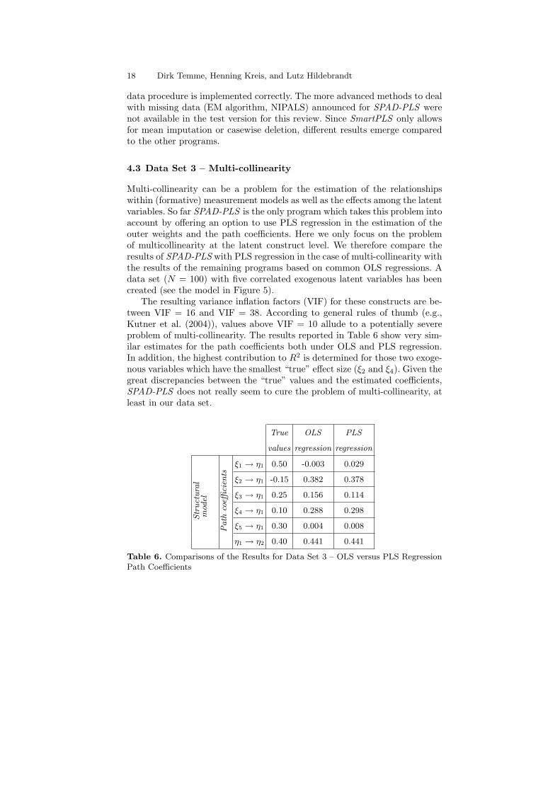
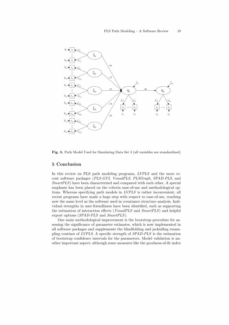
Multi-collinearity can be a problem for the estimation of the relationshipswithin (formative) measurement models as well as the effects among the latentvariables. So far SPAD-PLS is the only program which takes this problem intoaccount by offering an option to use PLS regression in the estimation of theouter weights and the path coefficients. Here we only focus on the problemof multicollinearity at the latent construct level. We therefore compare theresults of SPAD-PLS with PLS regression in the case of multi-collinearity withthe results of the remaining programs based on common OLS regressions. Adata set (N = 100) with five correlated exogenous latent variables has beencreated (see the model in Figure 5).

The resulting variance inflation factors (VIF) for these constructs are be-tween VIF = 16 and VIF = 38. According to general rules of thumb (e.g.,Kutner et al. (2004)), values above VIF = 10 allude to a potentially severeproblem of multi-collinearity. The results reported in Table 6 show very sim-ilar estimates for the path coefficients both under OLS and PLS regression.In addition, the highest contribution to R2 is determined for those two exoge-nous variables which have the smallest “true” effect size (ξ2 and ξ4). Given thegreat discrepancies between the “true” values and the estimated coefficients,SPAD-PLS does not really seem to cure the problem of multi-collinearity, atleast in our data set.

True OLS PLS

values regression regression

Str

uct

ura

lm

odel

Path

coeffi

cien

ts

ξ1 → η1 0.50 -0.003 0.029

ξ2 → η1 -0.15 0.382 0.378

ξ3 → η1 0.25 0.156 0.114

ξ4 → η1 0.10 0.288 0.298

ξ5 → η1 0.30 0.004 0.008

η1 → η2 0.40 0.441 0.441

Table 6. Comparisons of the Results for Data Set 3 – OLS versus PLS RegressionPath Coefficients


Fig. 5. Path Model Used for Simulating Data Set 3 (all variables are standardized)

5 Conclusion

In this review on PLS path modeling programs, LVPLS and the more re-cent software packages (PLS-GUI, VisualPLS, PLSGraph, SPAD-PLS, andSmartPLS ) have been characterized and compared with each other. A specialemphasis has been placed on the criteria ease-of-use and methodological op-tions. Whereas specifying path models in LVPLS is rather inconvenient, allrecent programs have made a huge step with respect to ease-of-use, reachingnow the same level as the software used in covariance structure analysis. Indi-vidual strengths in user-friendliness have been identified, such as supportingthe estimation of interaction effects (VisualPLS and SmartPLS ) and helpfulexport options (SPAD-PLS and SmartPLS ).

One main methodological improvement is the bootstrap procedure for as-sessing the significance of parameter estimates, which is now implemented inall software packages and supplements the blindfolding and jacknifing resam-pling routines of LVPLS. A specific strength of SPAD-PLS is the estimationof bootstrap confidence intervals for the parameters. Model validation is an-other important aspect; although some measures like the goodness-of-fit index


(Tenenhaus et al., 2005) have been discussed in the literature, so far only theblindfolding cross-validation indices (cv-redundancy and cv-communality) areoffered. The performance of the different programs has also been tested ondata sets with missing data and multi-collinearity. Here, both PLS-GUI andVisual-PLS provide an incorrect missing data code for the LVPLS input file.A major improvement in dealing with missing data is expected for the nextrelease of SPAD-PLS.

Multi-collinearity is a problem both for the estimation of weights in thecase of formative constructs and the estimation path coefficients. To cure thisproblem, SPAD-PLS has implemented a PLS regression routine. In our study,results for simulated data, however, are very similar to those resulting fromOLS regression. This issue should be the subject of a comprehensive MonteCarlo study.

Overall, there is considerable demand for implementations of the variousmethodological advances documented, for example, in this volume.

References

Allison, P. D. (2002). Missing Data. Sage, Thousand Oaks, CA.Chin, W. W. (1993-2003). PLS Graph – Version 3.0. Soft Modeling Inc.Chin, W. W. (2000). Frequently Asked Questions – Partial Least Squares &

PLS-Graph. http://disc-nt.cba.uh.edu/chin/plsfac.htm.Chin, W. W. (2001). PLS-Graph User’s Guide Version 3.0. C. T. Bauer

College of Business, University of Houston, Houston, Texas.Chin, W. W., Marcolin, B. L., and Newsted, P. N. (2003). A partial least

squares latent variable modeling approach for measuring interaction effects:Results from a monte carlo simulation study and an electronic-mail emo-tion/adoption study. Information Systems Research, 14(2):189–217.

Diamantopoulos, A. and Winklhofer, H. (2001). Index construction with for-mative indicators: an alternative to scale development. Journal of MarketingResearch, 38(2):269–277.

Fu, J.-R. (2006a). VisualPLS – Partial Least Square (PLS) Regression – AnEnhanced GUI for Lvpls (PLS 1.8 PC) Version 1.04. National KaohsiungUniversity of Applied Sciences, Taiwan, ROC.

Fu, J.-R. (2006b). VisualPLS – Partial Least Square (PLS) Regression – AnEnhanced GUI for Lvpls (PLS 1.8 PC) Version 1.04. http://www2.kuas.edu.tw/prof/fred/vpls/index.html.

Haitovsky, Y. (1968). Missing data in regression analysis. Journal of the RoyalStatistical Society, 30:67–82.

Hansmann, K.-W. and Ringle, C. M. (2004). SmartPLS Benutzerhandbuch.Universitat Hamburg, Hamburg.

Jarvis, C. B., MacKenzie, S. B., and Podsakoff, P. M. (2003). A criti-cal review of construct indicators and measurement model misspecifica-


tion in marketing and consumer research. Journal of Consumer Research,30(September):199–218.

Kutner, M. H., Nachtsheim, C. J., Neter, J., and Li, W. (2004). Applied LinearStatistical Models. McGraw-Hill/Irwin, Homewood, IL, 5 edition.

Li, Y. (2003). PLS-GUI User Manual – A Graphic User Interface for LVPLS(PLS-PC 1.8) – Version 1.0. University of South Carolina, Columbia, SC.

Li, Y. (2005). PLS-GUI – Graphic User Interface for Partial Least Squares(PLS-PC 1.8) – Version 2.0.1 beta. University of South Carolina, Columbia,SC.

Little, R. J. A. and Rubin, D. B. (2002). Statistical Analysis with MissingData. Wiley, Hoboken, NJ, 2 edition.

Lohmoller, J.-B. (1984). LVPLS Program Manual - Version 1.6. Zentralarchivfur Empirische Sozialforschung, Universitat zu Koln, Koln.

Lohmoller, J.-B. (1987). PLS-PC: Latent Variables Path Analysis with PartialLeast Squares - Version 1.8 for PCs under MS-DOS.

MacCallum, R. C. and Browne, M. W. (1993). The use of causal indicators incovariance structure models: Some practical issues. Psychologicval Bulletin,114:533–541.

MacKenzie, S. B., Podsakoff, P. M., and Jarvis, C. B. (2005). The problemof measurement model misspecification in behavioral and organizationalresearch and some recommended solutions. Journal of Applied Psychology,90(4):710–730.

McLachlan, J. and Peel, D. (2000). Finite Mixture Models. Wiley, New York.Nunnally, J. C. and Bernstein, I. H. (1994). Psychometric Theory. McGraw-

Hill, New York, 3 edition.Ringle, C. M., Wende, S., and Will, A. (2005). SmartPLS – Version 2.0.

Universitat Hamburg, Hamburg.Sellin, N. (1989). PLSPATH - Version 3.01. Application Manual. Universitat

Hamburg, Hamburg.Tenenhaus, M., Vinzi, V. E., Chatelin, Y.-M., and Lauro, C. (2005). PLS path

modeling. Computational Statistics and Data Analysis, 48(1):159–205.Test&Go (2006). Spad Version 6.0.0. Paris, France.Vinzi, V., Tenenhaus, M., and Chatelin, Y. (2004). ESIS-PLS software. In

Demonstration at Club PLS 2004 Meeting, Jouy-en-Josas, France.Wold, H. (1982). Soft modeling: The basic design and some extensions. In

Joreskog, K. G. and Wold, H., editors, Systems Under Indirect Observation.Part II, pages 1–54. North-Holland, Amsterdam.

Wold, H. (1985). Partial least squares. In Kotz, S. and Johnson, N. L., editors,Encyclopaedia of Statistical Sciences, Volume 6, pages 581–591. Wiley, NewYork.

SFB 649 Discussion Paper Series 2006

For a complete list of Discussion Papers published by the SFB 649, please visit http://sfb649.wiwi.hu-berlin.de.

001 "Calibration Risk for Exotic Options" by Kai Detlefsen and Wolfgang K. Härdle, January 2006.

002 "Calibration Design of Implied Volatility Surfaces" by Kai Detlefsen and Wolfgang K. Härdle, January 2006.

003 "On the Appropriateness of Inappropriate VaR Models" by Wolfgang Härdle, Zdeněk Hlávka and Gerhard Stahl, January 2006.

004 "Regional Labor Markets, Network Externalities and Migration: The Case of German Reunification" by Harald Uhlig, January/February 2006.

005 "British Interest Rate Convergence between the US and Europe: A Recursive Cointegration Analysis" by Enzo Weber, January 2006.

006 "A Combined Approach for Segment-Specific Analysis of Market Basket Data" by Yasemin Boztuğ and Thomas Reutterer, January 2006.

007 "Robust utility maximization in a stochastic factor model" by Daniel Hernández–Hernández and Alexander Schied, January 2006.

008 "Economic Growth of Agglomerations and Geographic Concentration of Industries - Evidence for Germany" by Kurt Geppert, Martin Gornig and Axel Werwatz, January 2006.

009 "Institutions, Bargaining Power and Labor Shares" by Benjamin Bental and Dominique Demougin, January 2006.

010 "Common Functional Principal Components" by Michal Benko, Wolfgang Härdle and Alois Kneip, Jauary 2006.

011 "VAR Modeling for Dynamic Semiparametric Factors of Volatility Strings" by Ralf Brüggemann, Wolfgang Härdle, Julius Mungo and Carsten Trenkler, February 2006.

012 "Bootstrapping Systems Cointegration Tests with a Prior Adjustment for Deterministic Terms" by Carsten Trenkler, February 2006.

013 "Penalties and Optimality in Financial Contracts: Taking Stock" by Michel A. Robe, Eva-Maria Steiger and Pierre-Armand Michel, February 2006.

014 "Core Labour Standards and FDI: Friends or Foes? The Case of Child Labour" by Sebastian Braun, February 2006.

015 "Graphical Data Representation in Bankruptcy Analysis" by Wolfgang Härdle, Rouslan Moro and Dorothea Schäfer, February 2006.

016 "Fiscal Policy Effects in the European Union" by Andreas Thams, February 2006.

017 "Estimation with the Nested Logit Model: Specifications and Software Particularities" by Nadja Silberhorn, Yasemin Boztuğ and Lutz Hildebrandt, March 2006.

018 "The Bologna Process: How student mobility affects multi-cultural skills and educational quality" by Lydia Mechtenberg and Roland Strausz, March 2006.

019 "Cheap Talk in the Classroom" by Lydia Mechtenberg, March 2006. 020 "Time Dependent Relative Risk Aversion" by Enzo Giacomini, Michael

Handel and Wolfgang Härdle, March 2006. 021 "Finite Sample Properties of Impulse Response Intervals in SVECMs with

Long-Run Identifying Restrictions" by Ralf Brüggemann, March 2006. 022 "Barrier Option Hedging under Constraints: A Viscosity Approach" by

Imen Bentahar and Bruno Bouchard, March 2006.

SFB 649, Spandauer Straße 1, D-10178 Berlin http://sfb649.wiwi.hu-berlin.de

This research was supported by the Deutsche

Forschungsgemeinschaft through the SFB 649 "Economic Risk".

023 "How Far Are We From The Slippery Slope? The Laffer Curve Revisited" by Mathias Trabandt and Harald Uhlig, April 2006.

024 "e-Learning Statistics – A Selective Review" by Wolfgang Härdle, Sigbert Klinke and Uwe Ziegenhagen, April 2006.

025 "Macroeconomic Regime Switches and Speculative Attacks" by Bartosz Maćkowiak, April 2006.

026 "External Shocks, U.S. Monetary Policy and Macroeconomic Fluctuations in Emerging Markets" by Bartosz Maćkowiak, April 2006.

027 "Institutional Competition, Political Process and Holdup" by Bruno Deffains and Dominique Demougin, April 2006.

028 "Technological Choice under Organizational Diseconomies of Scale" by Dominique Demougin and Anja Schöttner, April 2006.

029 "Tail Conditional Expectation for vector-valued Risks" by Imen Bentahar, April 2006.

030 "Approximate Solutions to Dynamic Models – Linear Methods" by Harald Uhlig, April 2006.

031 "Exploratory Graphics of a Financial Dataset" by Antony Unwin, Martin Theus and Wolfgang Härdle, April 2006.

032 "When did the 2001 recession really start?" by Jörg Polzehl, Vladimir Spokoiny and Cătălin Stărică, April 2006.

033 "Varying coefficient GARCH versus local constant volatility modeling. Comparison of the predictive power" by Jörg Polzehl and Vladimir Spokoiny, April 2006.

034 "Spectral calibration of exponential Lévy Models [1]" by Denis Belomestny and Markus Reiß, April 2006.

035 "Spectral calibration of exponential Lévy Models [2]" by Denis Belomestny and Markus Reiß, April 2006.

036 "Spatial aggregation of local likelihood estimates with applications to classification" by Denis Belomestny and Vladimir Spokoiny, April 2006.

037 "A jump-diffusion Libor model and its robust calibration" by Denis Belomestny and John Schoenmakers, April 2006.

038 "Adaptive Simulation Algorithms for Pricing American and Bermudan Options by Local Analysis of Financial Market" by Denis Belomestny and Grigori N. Milstein, April 2006.

039 "Macroeconomic Integration in Asia Pacific: Common Stochastic Trends and Business Cycle Coherence" by Enzo Weber, May 2006.

040 "In Search of Non-Gaussian Components of a High-Dimensional Distribution" by Gilles Blanchard, Motoaki Kawanabe, Masashi Sugiyama, Vladimir Spokoiny and Klaus-Robert Müller, May 2006.

041 "Forward and reverse representations for Markov chains" by Grigori N. Milstein, John G. M. Schoenmakers and Vladimir Spokoiny, May 2006.

042 "Discussion of 'The Source of Historical Economic Fluctuations: An Analysis using Long-Run Restrictions' by Neville Francis and Valerie A. Ramey" by Harald Uhlig, May 2006.

043 "An Iteration Procedure for Solving Integral Equations Related to Optimal Stopping Problems" by Denis Belomestny and Pavel V. Gapeev, May 2006.

044 "East Germany’s Wage Gap: A non-parametric decomposition based on establishment characteristics" by Bernd Görzig, Martin Gornig and Axel Werwatz, May 2006.

045 "Firm Specific Wage Spread in Germany - Decomposition of regional differences in inter firm wage dispersion" by Bernd Görzig, Martin Gornig and Axel Werwatz, May 2006.




046 "Produktdiversifizierung: Haben die ostdeutschen Unternehmen den Anschluss an den Westen geschafft? – Eine vergleichende Analyse mit Mikrodaten der amtlichen Statistik" by Bernd Görzig, Martin Gornig and Axel Werwatz, May 2006. 047 "The Division of Ownership in New Ventures" by Dominique Demougin and Oliver Fabel, June 2006. 048 "The Anglo-German Industrial Productivity Paradox, 1895-1938: A Restatement and a Possible Resolution" by Albrecht Ritschl, May 2006. 049 "The Influence of Information Costs on the Integration of Financial Markets: Northern Europe, 1350-1560" by Oliver Volckart, May 2006. 050 "Robust Econometrics" by Pavel Čížek and Wolfgang Härdle, June 2006. 051 "Regression methods in pricing American and Bermudan options using consumption processes" by Denis Belomestny, Grigori N. Milstein and Vladimir Spokoiny, July 2006. 052 "Forecasting the Term Structure of Variance Swaps" by Kai Detlefsen and Wolfgang Härdle, July 2006. 053 "Governance: Who Controls Matters" by Bruno Deffains and Dominique Demougin, July 2006. 054 "On the Coexistence of Banks and Markets" by Hans Gersbach and Harald Uhlig, August 2006. 055 "Reassessing Intergenerational Mobility in Germany and the United States: The Impact of Differences in Lifecycle Earnings Patterns" by Thorsten Vogel, September 2006. 056 "The Euro and the Transatlantic Capital Market Leadership: A Recursive Cointegration Analysis" by Enzo Weber, September 2006. 057 "Discounted Optimal Stopping for Maxima in Diffusion Models with Finite Horizon" by Pavel V. Gapeev, September 2006. 058 "Perpetual Barrier Options in Jump-Diffusion Models" by Pavel V. Gapeev, September 2006. 059 "Discounted Optimal Stopping for Maxima of some Jump-Diffusion Processes" by Pavel V. Gapeev, September 2006. 060 "On Maximal Inequalities for some Jump Processes" by Pavel V. Gapeev, September 2006. 061 "A Control Approach to Robust Utility Maximization with Logarithmic Utility and Time-Consistent Penalties" by Daniel Hernández–Hernández and Alexander Schied, September 2006. 062 "On the Difficulty to Design Arabic E-learning System in Statistics" by Taleb Ahmad, Wolfgang Härdle and Julius Mungo, September 2006. 063 "Robust Optimization of Consumption with Random Endowment" by Wiebke Wittmüß, September 2006. 064 "Common and Uncommon Sources of Growth in Asia Pacific" by Enzo Weber, September 2006. 065 "Forecasting Euro-Area Variables with German Pre-EMU Data" by Ralf Brüggemann, Helmut Lütkepohl and Massimiliano Marcellino, September 2006. 066 "Pension Systems and the Allocation of Macroeconomic Risk" by Lans Bovenberg and Harald Uhlig, September 2006. 067 "Testing for the Cointegrating Rank of a VAR Process with Level Shift and Trend Break" by Carsten Trenkler, Pentti Saikkonen and Helmut Lütkepohl, September 2006. 068 "Integral Options in Models with Jumps" by Pavel V. Gapeev, September 2006. 069 "Constrained General Regression in Pseudo-Sobolev Spaces with Application to Option Pricing" by Zdeněk Hlávka and Michal Pešta, September 2006.




070 "The Welfare Enhancing Effects of a Selfish Government in the Presence of Uninsurable, Idiosyncratic Risk" by R. Anton Braun and Harald Uhlig, September 2006. 071 "Color Harmonization in Car Manufacturing Process" by Anton Andriyashin, Michal Benko, Wolfgang Härdle, Roman Timofeev and Uwe Ziegenhagen, October 2006. 072 "Optimal Interest Rate Stabilization in a Basic Sticky-Price Model" by Matthias Paustian and Christian Stoltenberg, October 2006. 073 "Real Balance Effects, Timing and Equilibrium Determination" by Christian Stoltenberg, October 2006. 074 "Multiple Disorder Problems for Wiener and Compound Poisson Processes With Exponential Jumps" by Pavel V. Gapeev, October 2006. 075 "Inhomogeneous Dependency Modelling with Time Varying Copulae" by Enzo Giacomini, Wolfgang K. Härdle, Ekaterina Ignatieva and Vladimir Spokoiny, November 2006. 076 "Convenience Yields for CO2 Emission Allowance Futures Contracts" by Szymon Borak, Wolfgang Härdle, Stefan Trück and Rafal Weron, November 2006. 077 "Estimation of Default Probabilities with Support Vector Machines" by Shiyi Chen, Wolfgang Härdle and Rouslan Moro, November 2006. 078 "GHICA - Risk Analysis with GH Distributions and Independent Components" by Ying Chen, Wolfgang Härdle and Vladimir Spokoiny, November 2006. 079 "Do Individuals Recognize Cascade Behavior of Others? - An Experimental Study –" by Tim Grebe, Julia Schmid and Andreas Stiehler, November 2006. 080 "The Uniqueness of Extremum Estimation" by Volker Krätschmer, December 2006. 081 "Compactness in Spaces of Inner Regular Measures and a General Portmanteau Lemma" by Volker Krätschmer, December 2006. 082 "Probleme der Validierung mit Strukturgleichungsmodellen" by Lutz Hildebrandt and Dirk Temme, December 2006. 083 "Formative Measurement Models in Covariance Structure Analysis: Specification and Identification" by Dirk Temme and Lutz Hildebrandt, December 2006. 084 "PLS Path Modeling – A Software Review" by Dirk Temme, Henning Kreis and Lutz Hildebrandt, December 2006.




pls path modeling â€“ a software review - sfb 649 - humboldt

Documents