point-free program calculation - departamento de informática
TRANSCRIPT

Point-free Program Calculation
Manuel Alcino Pereira da Cunha
Departamento de Informatica
Escola de Engenharia
Universidade do Minho
2005
Dissertacao submetida a Universidade do Minho para obtencao do grau de
Doutor em Informatica, ramo de Fundamentos da Computacao

ii

Acknowledgments
First of all, I would like to thank Jose Bernardo Barros for accepting being my supervisor.Eventually, the supervision extended to many other issues besides research, and evolvedinto a friendship that I really treasure. Many tanks also to Jorge Sousa Pinto, who joinedthis “boat” half-way through, but whose great supervision was key to the conclusion ofthis work.
Many other people deserve scientific acknowledgment: Jose Nuno for making me apoint-free maniac; Bacelar for clarifying so many tricky questions; Jose Espırito-Santofor the valuable tip concerning the categorical abstract machine; Thorsten Altenkirchfor pointing out some relevant work concerning decidability of equality; and Jose andMiguel for helping me tuning the pointwise to point-free translation.
For making the department (and not only) such a fun place to be, thank you againZe, Jorge, and Becas, but also Paulo, Manuel, Carlos, Victor, Orlando, Joao, Nestor, andMane. To my friends, Xano, Luıs, and Paula, special thanks are due for all the supportand encouragement during this work. And for being so important (and so patient) inthis last year, Rosa definitively deserves a long and tender kiss. And by the way, tu esravissante!
Finally, I would like to thank my sisters, Angelina and Natalia, for being my biggestfans, and my parents, Gloria and Manuel, for raising me so wisely and for the uncondi-tional support in all aspects of my life. I love you all! To my grandparents, who I missso much, I dedicate this thesis.
This thesis was partially supported by FCT research project Pure under contractPOSI/ICHS/44304/2002.
iii

iv

“Since the beginning of the century, computational procedures have be-come so complicated that any progress by those means has become impos-sible, without the elegance which modern mathematicians have brought tobear on their research, and by means of which the spirit comprehends quicklyand in one step a great many computations.
It is clear that elegance, so vaunted and so aptly named, can have noother purpose . . .
Go to the roots of these calculations! Group the operations. Classifythem according to their complexities rather than their appearances! This, Ibelieve, is the mission of future mathematicians. This is the road on whichI am embarking in this work.”
Evariste Galois. From the preface to his final manuscript. 1832.
v

vi

Abstract
Due to referential transparency, functional programming is particularly appropriate forequational reasoning. In this thesis we reason about functional programs by calcula-tion, using a program calculus built upon two basic ingredients. The first is a set ofrecursion patterns that allow us to define recursive functions implicitly. These are en-coded as higher-order operators that encapsulate typical forms of recursion, such as thewell-known foldr operator on lists. The second is a point-free style of programming inwhich programs are expressed as combinations of simpler functions, without ever men-tioning their arguments. The basic combinators are derived from standard categoricalconstructions, and are characterized by a rich set of equational laws. In order to be ableto apply this calculational methodology to real lazy functional programming languages,a concrete category of partial functions and elements is used.
While recursion patterns are already well accepted and a lot of research has beencarried out on this topic, the same cannot be said about point-free programming. Thisthesis addresses precisely this component of the calculus. One of the contributions is amechanism to translate classic pointwise code into the point-free style. This mechanismcan be applied to a λ-calculus rich enough to represent the core functionality of a realfunctional programming language. A library that enables programming in a pure point-free style within Haskell is also presented. This library is useful for understanding theexpressions resulting from the above translation, since it allows their direct executionand, where applicable, the graphical visualization of recursion trees. Another contribu-tion of the thesis is a framework for performing point-free calculations with higher-orderfunctions. This framework is based on the internalization of some basic combinators,and considerably shortens calculations in this setting. In order to assess the viabilityof mechanizing calculations, several issues are discussed concerning the decidability ofequality and the implementation of fusion laws.
vii

viii

Resumo
Devido a transparencia referencial, o paradigma funcional e particularmente adequadoao raciocınio equacional. Nesta tese a manipulacao de programas funcionais sera feitapor calculo, sendo o calculo de programas constituido por dois ingredientes fundamen-tais. O primeiro e um conjunto de padroes de recursividade que nos permite definirfuncoes recursivas implicitamente. Estes padroes sao codificados como operadores deordem superior que ecapsulam formas de recursao tıpicas, tal como o bem conhecidooperador foldr para listas. O segundo ingrediente e um estilo de programacao “point-free”, no qual os programas sao definidos por combinacao de funcoes mais simples semnunca mencionar explicitamente os seus argumentos. Os combinadores fundamentaissao derivados de construcoes categoriais padrao, e sao caracterizados por um conjuntoexpressivo de leis equacionais. Para ser possıvel aplicar este metodo de calculo a lingua-gens de programacao funcional “lazy”, foi usada uma categoria concreta onde as funcoese os elementos podem ser parciais.
Ao contrario dos padroes de recursividade, que ja sao bem aceites e sobre os quais jase fez muita investigacao, o mesmo nao se pode dizer sobre a programacao “point-free”.Esta tese aborda precisamente este componente do calculo. Uma das contribuicoes e ummecanismo que permite traduzir codigo “pointwise” classico para o estilo “point-free”.Este mecanismo pode ser aplicado a um λ-calculus suficientemente expressivo para repre-sentar a funcionalidade basica de uma liguagem de programacao funcional real. Tambemse apresenta uma biblioteca que permite programar num estilo “point-free” puro dentroda linguagem Hankell. Esta biblioteca e util para compreender as expressoes que resul-tam da traducao acima referida, pois permite a sua execucao directa e, quando aplicavel,a visualizacao grafica de arvores de recursividade. Outra contribuicao da tese consistenuma metodologia para realizar calculos “point-free” sobre funcoes de ordem superior.Esta metodologia e baseada na internalizacao de alguns combinadores fundamentais,e permite encurtar significativamente os calculos. Para estabelecer a viabilidade demecanizacao, tambem se discutem varias questoes relacionadas com a decidibilidade daigualdade e a implementacao de leis de fusao.
ix

x

Contents
1 Introduction 1
2 Algebraic Programming 7
2.1 Some Categorical Notions . . . . . . . . . . . . . . . . . . . . . . . . . . 82.2 Basic Combinators . . . . . . . . . . . . . . . . . . . . . . . . . . . . . . 122.3 Recursive Data Types . . . . . . . . . . . . . . . . . . . . . . . . . . . . 212.4 Hylomorphisms . . . . . . . . . . . . . . . . . . . . . . . . . . . . . . . . 242.5 Summary . . . . . . . . . . . . . . . . . . . . . . . . . . . . . . . . . . . 29
3 Recursion Patterns as Hylomorphisms 31
3.1 Catamorphisms . . . . . . . . . . . . . . . . . . . . . . . . . . . . . . . . 323.1.1 Type Functors. . . . . . . . . . . . . . . . . . . . . . . . . . . . . 37
3.2 Anamorphisms . . . . . . . . . . . . . . . . . . . . . . . . . . . . . . . . 393.2.1 Splitting Hylomorphisms . . . . . . . . . . . . . . . . . . . . . . 43
3.3 Paramorphisms . . . . . . . . . . . . . . . . . . . . . . . . . . . . . . . . 433.4 Apomorphisms . . . . . . . . . . . . . . . . . . . . . . . . . . . . . . . . 483.5 Accumulations . . . . . . . . . . . . . . . . . . . . . . . . . . . . . . . . 503.6 Summary . . . . . . . . . . . . . . . . . . . . . . . . . . . . . . . . . . . 56
4 Calculating Accumulations Using Fusion 57
4.1 A Motivating Example . . . . . . . . . . . . . . . . . . . . . . . . . . . . 574.1.1 Transformation With Fold/Unfold Rules . . . . . . . . . . . . . . 584.1.2 Transformation by Calculation . . . . . . . . . . . . . . . . . . . 604.1.3 Transformation in the Point-free Style . . . . . . . . . . . . . . . 62
4.2 Calculating Accumulations in the Point-free Style . . . . . . . . . . . . . 664.2.1 Tail-recursive Accumulations over Lists . . . . . . . . . . . . . . 674.2.2 Other Accumulations over Lists . . . . . . . . . . . . . . . . . . . 714.2.3 Accumulations over Leaf-labeled Trees . . . . . . . . . . . . . . . 744.2.4 Accumulations over Rose Trees . . . . . . . . . . . . . . . . . . . 76
4.3 Functions with more than one accumulator . . . . . . . . . . . . . . . . 784.4 Transforming Hylomorphisms into Accumulations . . . . . . . . . . . . . 82
xi

xii Contents
4.5 Related Work . . . . . . . . . . . . . . . . . . . . . . . . . . . . . . . . . 83
4.6 Summary . . . . . . . . . . . . . . . . . . . . . . . . . . . . . . . . . . . 85
5 Mechanizing Fusion 87
5.1 Warm Fusion . . . . . . . . . . . . . . . . . . . . . . . . . . . . . . . . . 87
5.2 Cold Fusion: First Steps . . . . . . . . . . . . . . . . . . . . . . . . . . . 88
5.3 Higher-order Matching: the MAG System . . . . . . . . . . . . . . . . . 90
5.4 Fusion in the Point-free Style . . . . . . . . . . . . . . . . . . . . . . . . 92
5.5 Summary . . . . . . . . . . . . . . . . . . . . . . . . . . . . . . . . . . . 94
6 Pointless Haskell 95
6.1 Implementing the Basic Concepts . . . . . . . . . . . . . . . . . . . . . . 96
6.2 Programming with Explicit Functors . . . . . . . . . . . . . . . . . . . . 100
6.3 A Point-free Programming Library . . . . . . . . . . . . . . . . . . . . . 102
6.3.1 The PolyP Approach to Recursive Data Types . . . . . . . . . . 103
6.3.2 Polytypic Functor Instances . . . . . . . . . . . . . . . . . . . . 104
6.3.3 Implicit Coercion . . . . . . . . . . . . . . . . . . . . . . . . . . . 105
6.4 Visualization of Intermediate Data Structures . . . . . . . . . . . . . . . 110
6.4.1 Hood and GHood . . . . . . . . . . . . . . . . . . . . . . . . . . 110
6.4.2 Instrumenting Hylomorphisms for Visualization . . . . . . . . . . 113
6.4.3 Polytypic Observable Instances . . . . . . . . . . . . . . . . . . 116
6.5 Summary . . . . . . . . . . . . . . . . . . . . . . . . . . . . . . . . . . . 118
7 Deriving Point-free Definitions 121
7.1 Typed λ-Calculi and Cartesian Closed Categories . . . . . . . . . . . . . 121
7.2 Sums . . . . . . . . . . . . . . . . . . . . . . . . . . . . . . . . . . . . . . 126
7.3 Explicit Recursion . . . . . . . . . . . . . . . . . . . . . . . . . . . . . . 133
7.4 Deriving Hylomorphisms from Recursive Definitions . . . . . . . . . . . 136
7.5 Pattern Matching and Structured Types . . . . . . . . . . . . . . . . . . 142
7.6 Summary . . . . . . . . . . . . . . . . . . . . . . . . . . . . . . . . . . . 147
8 Decidability of Equality 149
8.1 Equational Reasoning and Term Rewriting Systems . . . . . . . . . . . 150
8.2 Normalization by Rewriting . . . . . . . . . . . . . . . . . . . . . . . . . 151
8.2.1 Expansionary Systems . . . . . . . . . . . . . . . . . . . . . . . . 152
8.2.2 Coping With Sums. . . . . . . . . . . . . . . . . . . . . . . . . . 153
8.3 Normalization by Evaluation . . . . . . . . . . . . . . . . . . . . . . . . 156
8.4 Normalization in the Point-Free Setting . . . . . . . . . . . . . . . . . . 159
8.5 Summary . . . . . . . . . . . . . . . . . . . . . . . . . . . . . . . . . . . 162

Contents xiii
9 Towards the Mechanization of Point-free Calculations 163
9.1 Birds’s Functional Calculator . . . . . . . . . . . . . . . . . . . . . . . . 1649.2 Scrap Your Boilerplate . . . . . . . . . . . . . . . . . . . . . . . . . . . . 166
9.2.1 Implementing Generic Transformations . . . . . . . . . . . . . . 1689.2.2 Generic Queries . . . . . . . . . . . . . . . . . . . . . . . . . . . . 1699.2.3 Monadic Transformations . . . . . . . . . . . . . . . . . . . . . . 170
9.3 A Typed Point-free Calculator . . . . . . . . . . . . . . . . . . . . . . . 1729.4 Simplification of Terms Translated from Pointwise . . . . . . . . . . . . 1759.5 Summary . . . . . . . . . . . . . . . . . . . . . . . . . . . . . . . . . . . 178
10 Conclusions and Future Work 179
A Additional Laws and Proofs 185

xiv Contents

Chapter 1
Introduction
Functional programming is particularly appropriate for equational reasoning. Due toreferential transparency, expressions in a functional programming language behave asordinary mathematical ones, meaning that expressions denoting the same value canbe interchanged without concern for the meaning of the surrounding context. Thisfact has been known for a long time, and put into practice for program reasoning atleast since Burstall and Darlington [BD77] introduced the fold/unfold technique, andBackus [Bac78] proposed his calculational methodology.
In fold/unfold program transformation one applies a number of semantically soundrules to an initial program, with the aim of arriving at a better, equivalent transformedprogram. “Better” here may have different interpretations: time and space complexityimprovements are obvious criteria, but removal of recursion is also a common goal(allowing to convert programs into purely iterative forms). This is an activity thatinvolves steps that are not easily automated, and as such typically requires humanintervention.
In this thesis we use a different framework for reasoning about functional programs:by calculation. Essentially a program calculus consists of a collection of equational lawsallowing to prove semantic equivalence between programs, or else to derive programsfrom other programs, or from their specifications. Quoting Backus [Bac78]:
Associated with the functional style of programming is an algebra of pro-grams [. . . ] This algebra can be used to transform programs and to solveequations whose “unknowns” are programs in much the same way one trans-forms equations in high-school algebra.
Some classic strategies for program transformation have been introduced using thisframework, such as Bird’s accumulation strategy [Bir84]. One advantage of the calcula-tional approach is that one can use the programming language itself to express propertiesand reason about the programs, rather than having a different formalism. Although not
1

2 Chapter 1: Introduction
so general as the fold/unfold technique, this approach is also easier to mechanize be-cause it only implies a local program analysis and the application of simple rewrite rules(typically with simple or no side conditions to verify), and since it does not require anyglobal analysis it can also be implemented in a modular way [THT98].
The program calculus used in this thesis is built upon two basic ingredients. Thefirst is a set of recursion patterns that allow us to define recursive functions implic-itly. These are encoded as higher-order operators that encapsulate typical forms ofrecursion such as the well-known foldr operator on lists. These operators enjoy a niceset of equational laws, and their importance to functional programming has been com-pared to the abandoning of arbitrary gotos in favor of structured control primitivesin the imperative setting. The second is a point-free style of programming in whichprograms are expressed as combinations of simpler functions, without ever mentioningtheir arguments. The calculus uses a reduced set of combinators, derived from standardcategorical constructions, again characterized by a rich set of equational laws. Sincethe choice of recursion patterns and point-free combinators was mainly driven by thepower of the associated laws, this programming paradigm is usually known as AlgebraicProgramming.
While recursion patterns are already widely used by functional programmers, thesame cannot be said about point-free programming. Although there are obvious ad-vantages in using this style – the absence of variables and λ-abstractions simplifies thepresentation and implementation of reduction rules – most authors still resort to point-wise, both for programming and for calculation, arguing that the intuitive meaningof point-free programs may be easily lost (it has even been jokingly called the point-less style). Quoting Jeremy Gibbons on the advantages of calculating in the point-freestyle [Gib99]:
This is the point of pointless calculations: when you travel light – discard-ing variables that do not contribute to the calculation – you can sometimesstep lightly across the surface of the quagmire.
Even if programmers were forced to program in the point-free style there wouldstill be a large amount of legacy code to which we would like to apply our reasoningmethodology. As such, in this thesis the point-free style will be used just for calculations,and we assume that the programs one wants to reason about are defined in pointwise. Auseful comparison here is that of mathematical transforms such as the Fourier transformor the Laplace transform, which allow to express functions in different domains in whichcertain manipulations are easier to perform.
This methodology raises a number of pertinent questions, most of them concerningthe point-free aspect of the paradigm. As said above, recursion patterns are already wellaccepted, and indeed a lot of research, both theoretical and practical, has been carried

3
out on this topic. One possible question could be: to what extent will calculations becommitted to the point-free style? Readers acquainted with the subject could point outthat when functions become a little more hairy, even the authors that clearly advocatethis style introduce some variables in order to simplify calculations. That is the casewith features nowadays so beloved such as curried or higher-order functions. To thisquestion we have a radical answer. Although we agree that some calculations can bevery long and tedious, we don’t think this is an intrinsic disadvantage of point-free, butmerely a consequence of the lack of adequate combinators and a solid proof methodology.As such, one of the objectives of this thesis is precisely to improve the machinery thatis used to perform point-free calculations, so that they can be done entirely within thisstyle.
Another question that immediately pops up is: how will pointwise code be trans-lated into point-free style? Interestingly, the need for such an algorithm was recentlymentioned in a functional programming mailing list, in a thread concerning the advan-tages/disadvantages of the point-free style [Kly05]:
[. . . ] it is easier to reason equationally with point-free programs, evenif the intended computation is often easier for mere mortals to see whennamed values are used. So point-free style helps when trying to apply programtransformation techniques, and translation to make greater use of point-freeidioms may be a useful precursor to transforming a program.
This question leads to another goal of this thesis: to define mechanisms to translatebetween pointwise and point-free, and vice-versa, so that the programmer is free tochoose whatever style is more adequate in any given context.
Once more, the above quotation reinforces what seems to be commonly accepted inthe functional programming community, but in fact we must also ask: is it really easyto reason about programs written in point-free style? This is obviously true if reasoningjust means the mechanical process of applying the equational laws as rewrite rules. Butthere are other (perhaps more) important issues concerning an equational theory, namelydecidability. Among the many authors who advocate point-free reasoning, we failed tofind a single one who addresses this issue, and found only a few who have attempted tomechanize proofs or transformations concerning point-free programs. So a third goal ofthe thesis is to help clarify this issue.
Another question that is relevant in any program reasoning and transformation con-text is: can this methodology be applied to real programming languages? The lastmain goal of the thesis is thus to answer this question positively. To be more specific,our target is the lazy functional programming language Haskell [Jon03]. As mentionedabove, the set of basic point-free combinators is derived from standard categorical con-structions. Most of the work presented here uses a concrete category of partial functions

4 Chapter 1: Introduction
and elements, that is typically used to give semantics to lazy programming languages.In practice, this means that the calculus is not so neat, and some laws are polluted bystrictness side conditions. This is the price to pay for using the appropriate semantics,which is not the case in most published work on this subject.
The thesis includes a large set of examples defined using recursion patterns and inthe point-free style. To emphasize the connection with Haskell, most of the examplesbegin with the equivalent definition given in this language. In program transformationexamples, that will also be the case with the transformed program. Finally, wheneverpossible, we tried to deploy our research results as practical tools and libraries thatoperate on Haskell programs instead of some abstract syntax. Haskell was also thelanguage of choice to develop them.
Overview of the Thesis.
Chapter 2 presents the foundations of the algebraic programming paradigm. It startswith a brief presentation of category theory. After enumerating the basic set of point-freecombinators and the associated laws, it describes how recursive types can be modeledin a categorical setting. Our presentation of recursion patterns differs slightly from theusual one. Given the concrete category underlying our presentation, we can assumethe existence of just one basic recursion pattern – the hylomorphism. This recursionpattern, whose presentation concludes Chapter 2, has an expressive power equivalentto that of the fixpoint operator. This expressiveness is put into use in Chapter 3,where hylomorphisms are used to define some of the best known recursion patterns,namely folds and unfolds. We also show how to derive their laws from the basic set thatcharacterizes hylomorphisms.
Some less known recursion patterns, such as paramorphisms or accumulations, arealso introduced in Chapter 3. Although these recursion patterns were originally definedusing folds, we show how they can be defined using hylomorphisms. This exercise revealsone of the advantages of using this recursion pattern. For some complex functions, adefinition using hylomorphisms is much easier to understand than one using just foldsor unfolds. In fact, a hylomorphism can be seen as the composition of a functionthat builds some intermediate data structure, and another one that consumes it. Thisproducer/consumer model usually simplifies the comprehension of the defined function.As such, hylomorphisms make an interesting contribution to program understanding.
The main contributions of the thesis start in Chapter 4. This chapter describes howBird’s accumulation strategy [Bir84] can be applied in a pure point-free setting. Themain problem with this technique is that it implements accumulations as higher-orderfolds that return a value of functional type (in Chapter 3 accumulations are definedin the uncurried form using tuple arguments). To simplify reasoning in this setting

5
some of the basic combinators introduced in Chapter 2 are internalized as point-freedefinitions. This approach allows us to derive some fairly advanced examples, namelyfunctions with two accumulating parameters. This chapter is a revised version of a paperto appear [CP05].
Many program transformation techniques, including Bird’s accumulation strategy,can be implemented using fusion. This law states the conditions in which the compo-sition of a function with a recursion pattern can be transformed into a single recursionpattern. Given its relevance, Chapter 5 presents a brief review of practical transforma-tion systems based on this law. As will be seen, there is already some solid work on theimplementation of fusion in the pointwise setting, but unfortunately very little on thepoint-free counterpart.
Some of the examples presented in the first chapters reinforce the idea that, indeed,it can be very difficult to program and understand definitions in the point-free style.Part of this problem could be alleviated if the programmer was able to execute and type-check his specifications. With this idea in mind, we have developed Pointless Haskell, alibrary that enables programming with recursion patterns in a pure point-free style. Theimplementation of this library is described in Chapter 6. The polytypic implementationof the recursion patterns is inherited from PolyP [NJ03], a generic programming libraryfor Haskell. With the help of some type system extensions, we have implemented an im-plicit coercion mechanism that provides a limited form of structural equivalence betweentypes. Although the library is embedded in Haskell, this mechanism allows us to use asyntax almost identical to the theoretical one defined in Chapter 2. This feature allowsfor a direct encoding of all the examples presented in this thesis. To further supportprogram understanding, the library also includes a generic visualization mechanism forthe intermediate data structures of hylomorphisms. This mechanism improves a previ-ous version developed for visualizing recursion trees of Haskell functions [Cun03], andis implemented using the graphical debugger GHood [Rei01].
Chapter 7 defines a mechanism to derive point-free hylomorphisms from explicitlyrecursive pointwise definitions. The chapter begins with the definition of a simply typedλ-calculus with pairs and terminal object, which is subsequently enriched with sums,explicit recursion, recursive data types, and pattern-matching. We believe that thesefeatures are rich enough to cover the core functionality of most functional programminglanguages, namely Haskell. The translation to point-free style is based on the well-knownequivalence between simply typed λ-calculi and cartesian closed categories suggested byLambek [Lam80]. We show how to extend this equivalence in order to cover sumsand the fixpoint operator. To handle sums we again resort to the internalization of aprimitive combinator. The fixpoint operator can be encoded as a hylomorphism, butsince this encoding yields expressions that are hard to manipulate, we also show howto adapt to our λ-calculus a well-known hylomorphism derivation algorithm that yields

6 Chapter 1: Introduction
more understandable definitions. None of these ingredients is entirely new, but, toour knowledge, it is the first time they are put together in order to build an effectivepointwise to point-free translation mechanism.
Chapter 8 presents a review of previous work on the decidability of equality inalmost bicartesian closed categories, i.e, categories with products, non-empty coproducts,exponentials and terminal object. Likewise to fusion mechanization, this problem isalready well studied at the pointwise level, but very few results exist for point-free.Namely, the problem has been shown to be decidable for pointwise terms using bothnormalization by rewriting and by evaluation. We show that a direct adaptation of thenormalization procedure based on an expansionary rewriting system to point-free termsis not possible.
In spite of the negative results presented, in practice it is easy to implement a systemthat, given some hints from the programmer, automates many point-free calculations.In Chapter 9 we review Bird’s functional calculator [Bir98], an example of one suchsystem. We show how it can be reimplemented using a generic programming library,and how it can be extended in order to accommodate type-directed expansion rules.The chapter concludes with the presentation of a rewriting system, that can be used tosimplify the point-free expressions that result from the translation defined in Chapter 7.
Chapter 10 begins with a review of the main contributions of the thesis. It alsodiscusses the proposed reasoning methodology taking into account the initially statedobjectives. The thesis ends with an enumeration of possible ideas for future work.

Chapter 2
Algebraic Programming
The origins of the algebraic programming paradigm can be traced back to 1977, whenJohn Backus proposed, in his ACM Turing Award lecture, a new functional style ofprogramming whose main features were the absence of variables and the use of functionalforms to combine existing functions into new functions [Bac78]. The main idea wasalready to develop a calculus of programs that could be used for program transformation.The choice of the functional forms was based not only on their programming power, butalso on the power of the associated algebraic laws. Most of the now standard combinators(presented later in this chapter) were already introduced in that seminal paper.
This approach was later endorsed by Bird and Meertens, who popularized a styleof programming (the so-called “Bird-Meertens formalism”) where final programs werederived from their specifications (typically, an inefficient combination of easy to un-derstand functions) through a set of equational laws [Bir84, Bir87, Mee86]. The nowwell-known notions of folding and fusion (or promotion) over lists were presented inthis work, enabling, for the first time, the effective use of the calculational approach inprogram transformation. The main difference with respect to the initial approach byBackus was the emphasis on the use of recursion operators, instead of the point-freecombinators. As Backhouse pointed out [Bac89], the importance of the Bird-Meertensformalism lies not on the foundational concepts per se (at the time already known), buton their application to develop a concise calculational method for program transforma-tion.
Malcolm later showed that the concepts introduced by Bird and Meertens (notablythe notion of fusion) arise naturally for any data type when viewed in a categoricalsetting [Mal90]. The categorical approach to data types, and functional programmingin general, had been previously clarified by Hagino [Hag87]; category theory turned outto be a natural setting for defining the basic building blocks of data types (includingsophisticated concepts such as mutually recursive data types, types defined using otherparameterized data types, and infinite data types). As shown in this chapter, the defini-
7

8 Chapter 2: Algebraic Programming
tion of most of the combinators used in the point-free style of programming is immediatefrom standard categorical constructions.
The generalization proposed by Malcolm was done in the context of total functionsand totally defined elements, but later Meijer, Fokkinga, and Paterson [MFP91] ex-tended it to the domain of partial functions and elements, thus enabling the powerof full recursion, and providing a more appropriate semantic domain to modern lazyprogramming languages.
Our presentation of algebraic programming will be split into two chapters. This onepresents the basic point-free combinators, the categorical approach to modeling recursivedata-types, and the notion of hylomorphism. This fundamental recursion pattern willbe used in the next chapter to implement typical recursion patterns, such as folds andunfolds.
2.1 Some Categorical Notions
The category theory concepts that will be used in this thesis are very simple, and arepresented in any introductory book to the subject, such as [Pie91]. Essentially, a categoryis a collection of objects and a collection of arrows (or morphisms), such that
• an arrow f with domain A and codomain B is denoted by f : A → B;
• there exists a composition operator · ◦ · that assigns to each pair of arrows g :A → B and f : B → C their composite arrow f ◦ g : A → C, and that obeys thefollowing associative law
f ◦ (g ◦ h) = (f ◦ g) ◦ h Comp-Assoc
• for each object A there exists an identity arrow idA : A → A satisfying the followingcondition
id ◦ f = f ◦ id = f Id-Nat
As seen in Id-Nat, we will often drop the typing information from most of the basic“polymorphic” morphisms, whenever this information can be easily derived from thecontext or is not relevant. In this case the complete formulation of the law would be:for any arrow f : A → B, we have idB ◦ f = f ◦ idA = f .
The following is another basic fact about any category.
f ◦ h = g ◦ h ⇐ f = g Leibniz
The categorical approach to functional programming is based on a categorical ac-count of the denotational semantics, with functions modeled by arrows in the underlyingcategory, and types modeled by objects in that category. A lot of the research done in

2.1 Some Categorical Notions 9
the area of algebraic programming is being carried out in the context of total functionsand total elements. Technically, this means that the model of computation is Set, thecategory where objects are sets and morphisms are total functions. Unfortunately, thiscategory is not a good semantic model for modern lazy functional languages, since ithardens the treatment of arbitrary recursive and partial definitions. Another problem isthat, in Set, finite and infinite data types are different entities that cannot be combined,thus excluding, for example, functions defined by induction that work for both, and alsothe hylomorphism recursion pattern that will be defined in Section 2.4.
These problems can be overcome by moving to the category CPO, which imposessome additional structure: objects are pointed complete partial orders, and morphismsare continuous functions (more details later). The study of algebraic programming in thissetting was pioneered by Meijer, Fokkinga and Paterson [MFP91], and the presentationof the material in this chapter is strongly influenced by their work.
A partial order (poset) is a set A that is equipped with a reflexive, transitive, andantisymmetric relation vA (we will drop the subscript if it is clear from the context).The least element of a poset A is the a ∈ A such that a v b for all b ∈ A (notice thatit may not exist, but if it exists, by antisymmetry it must be unique). A chain is asequence {ai | i ≥ 0} ⊆ A such that ∀i ≥ 0, ai v ai+1.
An upper bound of a chain {ai | i ≥ 0} is an element a such that ∀i ≥ 0, ai v a. Theleast upper bound (lub) is an upper bound that is less than or equal to every other upperbound. If a chain {ai | i ≥ 0} ⊆ A has a lub it is denoted by
⊔Ai≥0 ai. A poset where
every chain has a lub is a complete partial order (cpo). If it also has a least element(denoted by ⊥A) it is called a pointed complete partial order (pcpo).
A function f : A → B between pcpos A and B is monotonic if ∀a1, a2 ∈ A, ifa1 vA a2 then f a1 vB f a2. A monotonic function f : A → B is continuous if for eachchain {ai | i ≥ 0} ⊆ A it is the case that f (
⊔Ai≥0 ai) =
⊔Bi≥0(f ai).
Since types will be modeled by pcpos, this means that their elements can be com-pared according to a partial order v. The fact x v y will mean that x is an approxi-mation of y, in the sense that x is less well defined than y. Completeness of a partialorder implies that infinite data structures can be determined by the limit of their finiteapproximations. Continuity means that functions (modeled by arrows) respect theselimits.
Terminal Object. The terminal object in CPO is 1 = {⊥1}. This means that forany other object A there exists a unique arrow from it to 1, namely the function thatalways returns ⊥1. We will denote that arrow by !A. Since the least element of thefunctional type is precisely the function that always returns ⊥, !A denotes the value

10 Chapter 2: Algebraic Programming
⊥A→1. Given any f : A → B, ! is characterized by the following properties.
!1 = id1 Bang-Reflex
!B ◦f = !A Bang-Fusion
Points. Elements of a pcpo A are represented categorically by arrows of type 1 → A,usually called points. Given an element x ∈ A, x denotes the corresponding point in thecategory. By composing points with ! it is possible to define constant morphisms, thatignore the argument and always return a specific value.
Strictness. From the point of view of program calculation, the major difference be-tween using Set and CPO as the underlying category is that some of the laws that char-acterize the basic combinators will have strictness side conditions. As we will shortlysee, this is due to the fact that the separated sum is not a categorical coproduct inCPO. A function f : A → B is strict if it preserves bottoms. In the categorical setting,a strict morphism is defined as follows.
f strict ⇔ f ◦ ⊥ = ⊥ Strict-Def
The composition of two strict functions is necessarily strict.
f ◦ g strict ⇐ f strict ∧ g strict Strict-Comp
The reverse implication is not true in general, but the following holds due to monotony.
f strict ⇐ f ◦ g strict Comp-Strict
Sometimes we will also refer to the sub-category of CPO where all the functions arestrict. We will denote this category by CPO⊥.
Functors. Another useful categorical concept is that of a functor, which will be usedto model type constructors. A functor F is a mapping between categories (it mapsobjects to objects and arrows to arrows) such that
F f : F A → F B ⇐ f : A → B
F (f ◦ g) = F f ◦ F g Functor-Comp
F idA = idFA Functor-Id
For our purposes (and in general in the context of programming language semantics),endofunctors in CPO will be used, mapping types to types, and functions to functions.

2.1 Some Categorical Notions 11
The basic set of functors includes the identity functor Id, whose action on types isdefined as Id A = A, and on functions as Id f = f . It also includes the constant functor:given a type A, the functor A is defined on types as A B = A, and on functions asA f = idA.
A functor is locally continuous if, for all objects A and B, its action on functions oftype A → B is continuous. A functor F is strictness-preserving if, given a strict f , F f
is also strict (essentially, it should be a functor in CPO⊥).
A bifunctor ? is a mapping from a pair of categories to a category; in the presentcontext a bifunctor maps pairs of types to types, and pairs of functions to functions,verifying the conditions (infix notation is used):
f ? g : A ? B → C ? D ⇐ f : A → C ∧ g : B → D
(f ◦ g) ? (h ◦ k) = (f ? h) ◦ (g ? k) Bifunctor-Comp
idA ? idB = idA?B Bifunctor-Id
Given two monofunctors F and G and a bifunctor ?, a new monofunctor F ? G canbe defined by lifting ? as follows:
(F ? G) A = (F A) ? (G A)
(F ? G) f = (F f) ? (G f)
Given a type A, a monofunctor A? can also be defined by sectioning ?:
(A?) = A ? Id
This left-sectioning corresponds to treating as a constant the first parameter of thefunctor. Analogously, the right-sectioning of a bifunctor can also be defined.
Natural Transformations. A natural transformation η between functors F and G,denoted by η : F
.→ G, is a function that assigns to each type A an arrow ηA : F A → G A
such that, for any function f : A → B the following naturality condition holds.
G f ◦ ηA = ηB ◦ F f
Alternatively, we could say that for each f : A → B the following diagram commutes.
F AηA //
F f
��
G A
G f
��F B ηB
// G B

12 Chapter 2: Algebraic Programming
If each ηA is also an isomorphism then η is called a natural isomorphism. The conceptof natural transformation can be generalized to bifunctors.
2.2 Basic Combinators
In this section we will introduce a number of type constructors (such as products andcoproducts); each comes equipped with its own function combinators and laws for thesecombinators. In the categorical setting, type constructors are simply universal construc-tions (that can be generalized as functors), and the laws can all be derived from theiruniversal properties. Most of the laws presented in this chapter have trivial proofs.Some are presented in order to exemplify the calculational style used throughout thethesis, but the majority of them are omitted.
Products. The product of two types is defined as the cartesian product:
A×B = {(x, y) |x ∈ A, y ∈ B}
The ordering on the elements is defined as
(a, b) v (c, d) ⇔ a v c ∧ b v d
which means that the least element is ⊥A×B = (⊥A,⊥B).
On a product A×B the projections and the split function combinator (denoted by· M ·) can also be defined.
fstA×B (x, y) = x
sndA×B (x, y) = y(g M h) x = (g x, h x)
The fact that the cartesian product is a categorical product in CPO is justified by thefollowing uniqueness law.
f = g M h ⇔ fst ◦ f = g ∧ snd ◦ f = h Prod-Uniq
This law is also known as the universal law of products. Universal laws are usedin category theory to implicitly characterize entities. Instead of giving the explicitpointwise definitions, we could state that the product of two objects A and B is anobject A×B, together with a pair of projections fst : A×B → A and snd : A×B → B,such that for every object C, and arrows g : C → A and h : C → B, there existsexactly one arrow from C to A×B, denoted by gMh, that makes the following diagram

2.2 Basic Combinators 13
commute (uniqueness is signaled by a dashed line).
Cg
{{xxxxxxxxxh
##GGGGGGGGG
gMh�����
A A×Bfst
oosnd
// B
The implicit definition of products via their universal law turns out to be muchmore effective for program calculation than the explicit pointwise definition given before.Suppose one wants to prove the following very simple property about split.
fst M snd = id Prod-Reflex
Given its pointwise definition, the proof goes as follows.2666666666664
fst M snd = id
⇔ { η-expansion }(fst M snd) (x, y) = id (x, y)
⇔ {definition of · M · and id }(fst (x, y), snd (x, y)) = (x, y)
⇔ {definition of fst and snd }(x, y) = (x, y)
Using the universal law, we can avoid unfolding definitions, and the proof becomeseven more straightforward.26666664
fst M snd = id
⇔ {Prod-Uniq, with g = fst, h = snd, and f = id }fst ◦ id = fst ∧ snd ◦ id = snd
⇔ { Id-Nat }fst = fst ∧ snd = snd
Throughout the thesis, the following conventions will be adopted. Although natural-ity of identity is explicitly mentioned here, it will usually be omitted. We will implicitlyuse associativity laws, just by omitting parenthesis around operators that enjoy thisproperty, namely composition. We will also assume that this operator binds strongerthan any other combinator in order to avoid the proliferation of parentheses.
Using Prod-Uniq the following laws can easily be proved.
fst ◦ (f M g) = f ∧ snd ◦ (f M g) = g Prod-Cancel
(f M g) ◦ h = f ◦ h M g ◦ h Prod-Fusion
f M g = h M i ⇔ f = h ∧ g = i Prod-Equal
It is also useful to define a product function combinator as follows.
f × g = f ◦ fst M g ◦ snd Prod-Def

14 Chapter 2: Algebraic Programming
Observe that this definition of product over functions allows to see product as a bifunc-tor. The corresponding laws can be checked as shown.
id× id = id Prod-Functor-Id
26666664id× id
= {Prod-Def }id ◦ fst M id ◦ snd
= {Prod-Reflex }id
(f × g) ◦ (h× i) = f ◦ h× g ◦ i Prod-Functor-Comp
266666666666666664
(f × g) ◦ (h× i)
= {Prod-Def }(f ◦ fst M g ◦ snd) ◦ (h ◦ fst M i ◦ snd)
= {Prod-Fusion }f ◦ fst ◦ (h ◦ fst M i ◦ snd) M g ◦ snd ◦ (h ◦ fst M i ◦ snd)
= {Prod-Cancel }f ◦ h ◦ fst M g ◦ i ◦ snd
= {Prod-Def }f ◦ h× g ◦ i
The following absorption law fuses a product with a split.
(f × g) ◦ (h M i) = f ◦ h M g ◦ i Prod-Absor
Since we are working in CPO it is important to characterize the strictness of thesplit combinator and the projections.
(f M g) strict ⇔ f strict ∧ g strict Prod-Strict
fst strict Fst-Strict
snd strict Snd-Strict
An example of a very useful function defined using split is the swap function.
swap : A×B → B ×A
swap = snd M fstSwap-Def
This function is a natural isomorphism between the bifunctor ·×· and A⊗B = B×A,as shown in the following calculations.
(f × g) ◦ swap = swap ◦ (g × f) Swap-Nat
swap ◦ swap = id Swap-Iso

2.2 Basic Combinators 15
26666666666666666666664
swap ◦ (g × f)
= {Swap-Def, Prod-Def }(snd M fst) ◦ (g ◦ fst M f ◦ snd)
= {Prod-Fusion, Prod-Cancel }f ◦ snd M g ◦ fst
= {Prod-Cancel }f ◦ fst ◦ (snd M fst) M g ◦ snd ◦ (snd M fst)
= {Prod-Fusion }(f ◦ fst M g ◦ snd) ◦ (snd M fst)
= {Swap-Def, Prod-Def }(f × g) ◦ swap
266666666666666664
swap ◦ swap
= {Swap-Def }(snd M fst) ◦ (snd M fst)
= {Prod-Fusion }snd ◦ (snd M fst) M fst ◦ (snd M fst)
= {Prod-Cancel }fst M snd
= {Prod-Reflex }id
Another useful natural isomorphism is the one that gives evidence of the associativityof the cartesian product.
assocr : (A×B)× C → A× (B × C)assocr = (fst ◦ fst) M (snd× id)
Assocr-Def
(f × (g × h)) ◦ assocr = assocr ◦ ((f × g)× h) Assocr-Nat
Its inverse is defined as follows.
assocl : A× (B × C) → (A×B)× C
assocl = (id× fst) M (snd ◦ snd)Assocl-Def
assocr ◦ assocl = assocl ◦ assocr = id Assocr-Iso
Sums. It is know that CPO does not have true coproducts. In most lazy functionallanguages this notion is implemented by the separated sum, where a new bottom elementis added to the tagged reunion of the elements of both sets.
A + B = ({0} ×A) ∪ ({1} ×B) ∪ {⊥A+B}
The ordering relation of this pcpo is defined as follows.
x v y ⇔ x = ⊥ ∨ (fst x = fst y ∧ snd x v snd y)
Dually to products, injections and the either combinator (denoted by · O ·) can bedefined on a sum A + B.
inlA+B x = (0, x)inrA+B x = (1, x)
(g O h) ⊥ = ⊥(g O h) (0, x) = g x
(g O h) (1, x) = h x

16 Chapter 2: Algebraic Programming
The fact that the separated sum is not a categorical coproduct in CPO is reflectedin the uniqueness law, that only holds for strict functions:
f = g O h ⇔ f ◦ inl = g ∧ f ◦ inr = h ∧ f strict Sum-Uniq
If the strictness side condition was omitted, the equation would not be valid becausethe right-hand side would not determine the outcome of f when applied to ⊥. Resortingto diagrams, we could say that there exists exactly one strict arrow from A + B to C
that makes the following diagram commute.
Ainl //
g##FFFFFFFFF A + B
gOh
����� B
inroo
h{{wwwwwwwww
C
Using uniqueness the following laws can be proved. Notice how fusion becomes“polluted” by strictness side conditions.
inl O inr = id Sum-Reflex
(f O g) ◦ inl = f ∧ (f O g) ◦ inr = g Sum-Cancel
f ◦ (g O h) = f ◦ g O f ◦ h ⇐ f strict Sum-Fusion
f O g = h O i ⇔ f = h ∧ g = i Sum-Equal
Likewise products, the separated sum can be turned into a bifunctor by defining itsoperation on arrows, which leads to the introduction of the sum function combinator:
f + g = inl ◦ f O inr ◦ g Sum-Def
Here are the corresponding functor and absorption laws.
id + id = id Sum-Functor-Id
(f + g) ◦ (h + i) = f ◦ h + g ◦ i Sum-Functor-Comp
(f O g) ◦ (h + i) = f ◦ h O g ◦ i Sum-Absor
By definition, any either is strict. However, unlike fst and snd, which are strictfunctions, inl and inr are not.
(f O g) strict Sum-Strict
There is an interesting law that relates split with either, typically called the abidesor exchange law.
(f M g) O (h M i) = (f O h) M (g O i) Abides

2.2 Basic Combinators 17
266666666666666664
(f M g) O (h M i)
= {Prod-Reflex }(fst M snd) ◦ ((f M g) O (h M i))
= {Prod-Fusion }fst ◦ ((f M g) O (h M i)) M snd ◦ ((f M g) O (h M i))
= {Sum-Fusion, Fst-Strict, Snd-Strict }(fst ◦ (f M g) O fst ◦ (h M i)) M (snd ◦ (f M g) O snd ◦ (h M i))
= {Prod-Cancel }(f O h) M (g O i)
Analogously to the swap function for products, the coswap can be defined for sums,with similar laws (and proofs).
coswap : A + B → B + A
coswap = inr O inlCoswap-Def
(f + g) ◦ coswap = coswap ◦ (g + f) Coswap-Nat
coswap ◦ coswap = id Coswap-Iso
Sum is also associative, and the isomorphism is justified by the following definitions.
coassocr : (A + B) + C → A + (B + C)coassocr = (id + inl) O (inr ◦ inr)
Coassocr-Def
coassocl : A + (B + C) → (A + B) + C
coassocl = (inl ◦ inl) O (inr + id)Coassocl-Def
Unfortunately, CPO is not a distributive category, which means that A × (B + C)is not isomorphic to (A × B) + (A × C). In fact, there are more elements in the firsttype (for example, given a value (x,⊥) of the first type, it must be converted into ⊥ ofthe second, but there is no way to invert this value in order to obtain the original x).Even so, it is possible to write a function that distributes the product over the sum andvice-versa. The point-free definition of the former needs exponentials, but the latter canbe readily defined as follows.
undistr : (A×B) + (A× C) → A× (B + C)undistr = (id× inl) O (id× inr)
Undistr-Def
Exponentials. The exponentiation of type B to type A is defined as the set of allfunctions with domain A and codomain B:
BA = {f | f : A → B}

18 Chapter 2: Algebraic Programming
Given pcpos A and B, the ordering of the continuous functions from A to B is determinedby
f v g ⇔ (f a v g a,∀a ∈ A)
As already mentioned in the previous section, this ordering implies that the least elementof BA is the function that always returns ⊥B.
Associated to the exponential BA, are the apply function and the curry combinator(denoted by · ).
apBA (f, x) = f x
g x y = g (x, y)
The following uniqueness law states that this notion of exponentiation is truly categoricalin CPO.
f = g ⇔ g = ap ◦ (f × id) Exp-Uniq
Alternatively, we could say that for every object C, and g : C × A → B, g is theunique arrow from C to BA that makes the following diagram commute.
BA ×Aap // B
C ×A
g
;;wwwwwwwwwg×id
OO���
The definition of the exponentiation combinator allows to turn this operation into afunctor:
fA = f ◦ ap Exp-Def
Notice that when the type in superscript is not relevant the symbol • will be used inreplacement. The following laws characterize exponentiation.
ap = id Exp-Reflex
ap ◦ (f × id) = f Exp-Cancel
f ◦ g = f ◦ (g × id) Exp-Fusion
f = g ⇔ f = g Exp-Equal
id• = id Exp-Functor-Id
(f ◦ g)• = f• ◦ g• Exp-Functor-Comp
f• ◦ g = f ◦ g Exp-Absor
Left-strictness. To characterize the strictness of the curry operator, the strongernotion of left-strictness is needed. An arrow of type A×B → C is left-strict if it returns

2.2 Basic Combinators 19
⊥C when the first element of the input pair is ⊥A. Categorically, this concept can becharacterized as follows.
f left-strict ⇔ f ◦ (⊥× id) = ⊥ ◦ fst Lstrict-Def
f strict ⇐ f left-strict Lstrict-Strict
Alternatively, f is left-strict iff the following diagram commutes.
1×Bfst //
⊥×id
��
1
⊥��
A×Bf
// C
An example of a strict function that is not left-strict is the projection snd.
Left-strictness and composition interact according to the following laws. Again, thelast law can be derived from monotony.
f ◦ (g × id) left-strict ⇐ f left-strict ∧ g strict Lstrict-Comp-Left
f ◦ g left-strict ⇐ f strict ∧ g left-strict Lstrict-Comp-Right
f left-strict ⇐ f ◦ (g × id) left-strict Comp-Lstrict
Remember that the least element of type AB is a function that ignores its argumentand always returns the least element of type A. As such, a curried function is strictif and only if its uncurried version is left-strict. The same reason justifies that ap is aleft-strict function (and thus strict).
f strict ⇔ f left-strict Exp-Strict
ap left-strict Ap-Lstrict
Distributivity. Using exponentials, functions to distribute products over sums canbe defined in the point-free style as follows.
distl : (A + B)× C → (A× C) + (B × C)distl = ap ◦ ((inl O inr)× id)
Distl-Def
distr : A× (B + C) → (A×B) + (A× C)distr = (swap + swap) ◦ distl ◦ swap
Distr-Def
Although CPO is not distributive, it is still true that
distr ◦ undistr = id Distr-Iso-Left

20 Chapter 2: Algebraic Programming
as the following calculation shows.
2666666666666666666666666666666666666666664
distr ◦ undistr
= {Distr-Def, Distl-Def, Undistr-Def }(swap + swap) ◦ ap ◦ ((inl O inr)× id) ◦ swap ◦ ((id× inl) O (id× inr))
= {Sum-Fusion, swap strict, Swap-Nat }(swap + swap) ◦ ap ◦ ((inl O inr)× id) ◦ ((inl× id) ◦ swap O (inr × id) ◦ swap)
= {Sum-Absor, Prod-Def }(swap + swap) ◦ ap ◦ ((inl O inr)× id) ◦ ((inl ◦ fst M snd) O (inr ◦ fst M snd)) ◦ (swap + swap)
= {Abides, Prod-Absor }(swap + swap) ◦ ap ◦ ((inl O inr) ◦ (inl ◦ fst O inr ◦ fst) M (snd O snd)) ◦ (swap + swap)
= {Sum-Fusion, Sum-Strict, Sum-Cancel }(swap + swap) ◦ ap ◦ ((inl ◦ fst O inr ◦ fst) M (snd O snd)) ◦ (swap + swap)
= {Abides, Prod-Def }(swap + swap) ◦ ap ◦ ((inl× id) O (inr × id)) ◦ (swap + swap)
= {Sum-Fusion, ap strict, Exp-Cancel }(swap + swap) ◦ (inl O inr) ◦ (swap + swap)
= {Sum-Reflex, Sum-Functor-Comp }swap ◦ swap + swap ◦ swap
= {Swap-Iso, Sum-Functor-Id }id
Obviously, the inverse does not hold (although undistr ◦ distr v id). Some additionalproperties about distributivity, namely naturality, are stated and proved in Appendix A.
Guards. Booleans can be defined by Bool = 1 + 1, with
true : 1 → Bool
true = inl
false : 1 → Bool
false = inr
Given this definition, negation is implemented by the coswap function.
To facilitate the point-free treatment of conditional expressions, it is useful to definethe guard combinator associated to a given predicate p : A → Bool.
p? : A → A + A
p? = (fst + fst) ◦ distr ◦ (id M p)Guard-Def
Notice that if p returns ⊥ for some input, then p? will also return ⊥.
Cartesian Closed Categories. A category that has products, exponentials, andterminal object is called cartesian closed. In these categories, the set of arrows from A
to B can be represented by the object BA. Formally, this means that an f : A → B canbe internalized as a point f : 1 → BA, and vice versa. Moreover, it is possible to definethe conversions between a function and its point using the basic combinators previously
2.3 Recursive Data Types 21
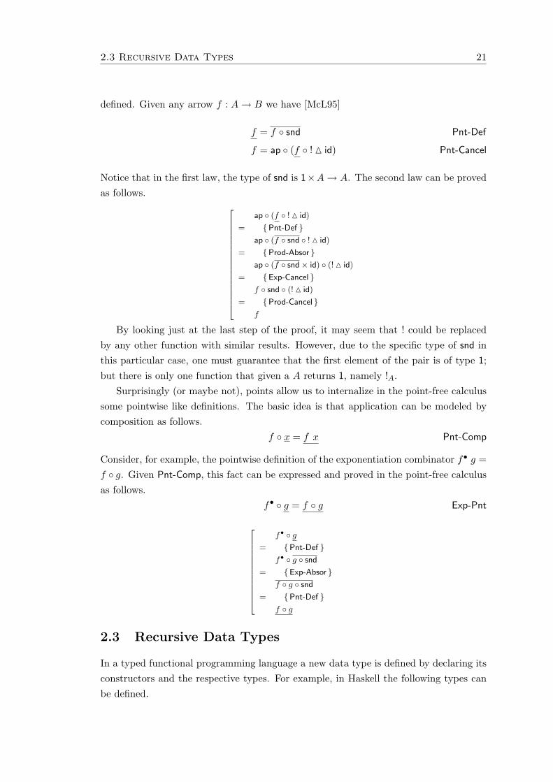
defined. Given any arrow f : A → B we have [McL95]
f = f ◦ snd Pnt-Def
f = ap ◦ (f ◦ ! M id) Pnt-Cancel
Notice that in the first law, the type of snd is 1×A → A. The second law can be provedas follows. 266666666666666664
ap ◦ (f ◦ ! M id)
= {Pnt-Def }ap ◦ (f ◦ snd ◦ ! M id)
= {Prod-Absor }ap ◦ (f ◦ snd× id) ◦ (! M id)
= {Exp-Cancel }f ◦ snd ◦ (! M id)
= {Prod-Cancel }f
By looking just at the last step of the proof, it may seem that ! could be replacedby any other function with similar results. However, due to the specific type of snd inthis particular case, one must guarantee that the first element of the pair is of type 1;but there is only one function that given a A returns 1, namely !A.
Surprisingly (or maybe not), points allow us to internalize in the point-free calculussome pointwise like definitions. The basic idea is that application can be modeled bycomposition as follows.
f ◦ x = f x Pnt-Comp
Consider, for example, the pointwise definition of the exponentiation combinator f• g =f ◦ g. Given Pnt-Comp, this fact can be expressed and proved in the point-free calculusas follows.
f• ◦ g = f ◦ g Exp-Pnt
2666666666664
f• ◦ g
= {Pnt-Def }f• ◦ g ◦ snd
= {Exp-Absor }f ◦ g ◦ snd
= {Pnt-Def }f ◦ g
2.3 Recursive Data Types
In a typed functional programming language a new data type is defined by declaring itsconstructors and the respective types. For example, in Haskell the following types canbe defined.

22 Chapter 2: Algebraic Programming
data Nat = Zero | Succ Nat
data List a = Nil | Cons a (List a)
data Tree a = Empty | Node a (Tree a) (Tree a)
The first one is a monomorphic type that represents natural numbers, and the laterare polymorphic ones representing lists and binary trees containing elements of an ar-bitrary type.
In order to present a general theory for data types, we first have to circumventsome “irregularities” in constructor declaration, namely, the fact that there may existan arbitrary number of constructors, and that each may have an arbitrary number ofarguments. This last problem is easily solved by treating constants as functions withdomain 1, and by uncurrying constructors with more than one parameter. For naturalsand lists this technique can be illustrated by the following declarations.
zero : 1 → Nat
succ : Nat → Nat
nil : 1 → List A
cons : A× List A → List A
For binary trees we have to decide where to put parentheses.
empty : 1 → Tree A
node : A× (Tree A× Tree A) → Tree A
All the constructors of a data type share the same target type. As such, the eithercombinator can be used to pack all of them in a single declaration, as in the followingdeclaration for naturals.
zero O succ : 1 + Nat → Nat
Since the domain is an expression involving the target type, the categorical concept offunctor can be used to factor this type out. The packed representation of the constructorsof a data type T will be denoted by inT , and the base functor that captures its signatureby FT . Notice that with this approach, the type of inT is always FT T → T . Forpolymorphic data types the type variables will be omitted in subscripts in order toimprove readability.
FNat = 1 + Id
inNat = zero O succ
FList = 1 + A × Id
inList = nil O cons
FTree = 1 + A × (Id × Id)inTree = empty O node
A recursive data type T is then defined by taking the fixed point of its base functorFT . Reynolds proved that in CPO, given a locally continuous and strictness-preservingbase functor F , there exists a unique data type T = µF and two unique strict functions

2.3 Recursive Data Types 23
inT : F T → T and outT : T → F T that are each other’s inverse [Rey77].
inT ◦ outT = idT ∧ outT ◦ inT = idFT In-Out-Iso
inT strict In-Strict
outT strict Out-Strict
Fokkinga and Meijer [FM91] showed that all polynomial, and even all regular func-tors, are locally continuous and strictness-preserving. A polynomial functor is either theidentity functor, a constant functor, a lifting of the sum and product bifunctors, or thecomposition of polynomial functors. This guarantees that, for example, all the followingdata types are well defined.
Nat = µ(FNat) List A = µ(FList) Tree A = µ(FTree)
A regular functor can also be built from type functors, a concept that will be presentedlater in Section 3.1.1. An example of a data type built from a regular functor is that ofrose trees, where each node may have an arbitrary number of children. Since all functorsused in this thesis are locally continuous and strictness-preserving, this fact will usuallybe omitted from proofs.
To see what elements belong to a data type defined by fixed point, let us take thenatural numbers as an example. A pcpo that satisfies the equation Nat ∼= 1 + Nat caninformally be defined as Nat = 1 + (1 + (1 + . . .)). We can picture the ordering relationof this pcpo as follows.
zero ⊥1 (succ ◦ zero) ⊥1 (succn ◦ zero) ⊥1
⊥Nat//
OO
succ ⊥Nat//
OO
(succn) ⊥Nat//
OO
∞
The elements in the upper row can be interpreted as the natural numbers, that is,0 = zero ⊥1, 1 = (succ ◦ zero) ⊥1, and in general n = (succn ◦ zero) ⊥1. Notice that theorder in the poset is a definedness order, and so, these elements are unrelated. Besidesthe natural numbers, Nat also contains a chain of “partial numbers”. An upper boundof this chain ∞ =
⊔n((succn) ⊥Nat) must be added in order to make the poset complete.
This element satisfies ∞ = succ ∞, and denotes the infinite number. Similarly, the datatype List A contains, not only all totally defined finite lists, but also chains of partial listswith shape cons (a0, cons (a1, . . .⊥)), whose upper bounds are totally defined infinitelists.
We have already seen what the in functions for this data types are. But what abouttheir destructors, the out functions? Given a predicate iszero : Nat → Bool that testsif a natural is equal to zero, and a function pred : Nat → Nat that determines the

24 Chapter 2: Algebraic Programming
predecessor, we have for naturals
outNat : Nat → 1 + Nat
outNat = (! + pred) ◦ iszero?
For lists, given a similar predicate isnil : List A → Bool, and the typical destructorshead : List A → A and tail : List A → List A we have
outList : List A → 1 + A× List A
outList = (! + (head M tail)) ◦ isnil?
Remark. This presentation excludes non-regular data types and mutually recursiveones. Several authors have shown how to extend this theory of algebraic programmingto mutually recursive data types [Mei92, SF93, IHT98]. There is also some work onextending it to nested data types [BP99, MG01]. These are parameterized data typesin which the parameter changes in the recursive call, and are interesting because theycan capture some structural invariants. For example, the following Haskell data typecan be used to store perfectly balanced binary trees with labels in the leafs.
data Balanced a = Leaf a | Fork (Balanced (a,a))
2.4 Hylomorphisms
The hylomorphism recursion pattern was first defined in [FM91]. Given a functor F , afunction g : F B → B, and a function h : A → F A, a hylomorphism is defined as thefollowing recursive function, using the fixpoint operator µ.
[[g, h]]µF : A → B
[[g, h]]µF = µ(λf.g ◦ Ff ◦ h)Hylo-Def
The main advantage of expressing recursive functions as hylomorphisms is that theyhave several interesting laws appropriate for program calculation and transformation.For example, by unfolding the fixpoint operator we immediately get the following can-cellation law.
[[g, h]]µF = g ◦ F [[g, h]]µF ◦ h Hylo-Cancel
From this law, it is clear that the recursion pattern of the hylomorphism is characterizedby the functor F . For example, if this functor is 1 + Id then the resulting definition isnecessarily linear recursive. To define a birecursive function a second degree polynomialfunctor, such as 1+ Id× Id, must be used. In fact, the recursion tree of a function definedas a hylomorphism is modeled by µF .
Function h is responsible for all computations prior to recursion, namely, to computethe values passed to the recursive calls. Function g combines the results of the recursive

2.4 Hylomorphisms 25
calls in order to compute the final result. Notice that some values can be passed intactfrom h to g. This will be the case when a functor modeling a data type that stores someinformation in the nodes is used, like 1 + A × Id for the case of lists.
Example 2.1 (Factorial). Consider the following typical definition of the factorialfunction in Haskell, where Nat is the data type defined in the previous section, andmult :: (Nat,Nat) -> Nat implements multiplication.
fact :: Nat -> Nat
fact Zero = Succ Zero
fact (Succ n) = mult (Succ n, fact n)
Assuming that constants are functions from 1, this recursive definition verifies thefollowing equations.
fact (zero ⊥) = succ (zero ⊥) ∧ fact (succ n) = mult (succ n, fact n)
By applying the definitions of composition and the split combinator we can push thevariables out of the expressions. one will be used as a shortcut to succ ◦ zero.
(fact ◦ zero) ⊥ = one ⊥ ∧ (fact ◦ succ) n = (mult ◦ (succ M fact)) n
η-reduction then enables us to transform these equations into the point-free style.
fact ◦ zero = one ∧ fact ◦ succ = mult ◦ (succ M fact)
With some simple calculations we can rearrange this expression as follows.266666666666666664
fact ◦ zero = one ∧ fact ◦ succ = mult ◦ (succ M fact)
⇔ {Sum-Equal }fact ◦ zero O fact ◦ succ = one O mult ◦ (succ M fact)
⇔ {Sum-Fusion, fact strict, Prod-Absor }fact ◦ (zero O succ) = one O mult ◦ (id× fact) ◦ (succ M id)
⇔ { inNat = zero O succ, Sum-Absor }fact ◦ inNat = (one O mult) ◦ (id + id× fact) ◦ (id + succ M id)
⇔ { In-Out-Iso }fact = (one O mult) ◦ (id + id× fact) ◦ (id + succ M id) ◦ outNat
This means that factorial can be determined by the fixpoint
fact = µ(λf.(one Omult) ◦ (FList f) ◦ (id + succ M id) ◦ outNat)
and hence defined as the hylomorphism
fact : Nat → Nat
fact = [[one Omult, (id + succ M id) ◦ outNat]]List Nat

26 Chapter 2: Algebraic Programming
Example 2.2 (Length). To give another example, this informal method to derive ahylomorphism will be applied to the following function that determines the length of alist.
length :: List a -> Nat
length Nil = Zero
length (Cons h t) = Succ (length t)
This definition satisfies the following pointwise equations.
length (nil ⊥) = zero ⊥ ∧ length (cons (h, t)) = succ (length t)
These can be converted into point-free style by using snd to “forget” the head of thelist.
length ◦ nil = zero ∧ length ◦ cons = succ ◦ length ◦ snd
By similar calculations to the factorial example, these equations can be converted into
length = inNat ◦ (id + length) ◦ (id + snd) ◦ outList
which means that length can be defined as the following hylomorphism.
length : List A → Nat
length = [[inNat, (id + snd) ◦ outList]]Nat
Laws. Most of the fundamental laws about hylomorphisms follow directly from similarlaws about fixpoints, or can be proved by fixpoint induction. That is the case of thefollowing, first presented in [FM91].
g ◦ [[h, i]]µF ◦ j = [[k, l]]µF
⇐g strict ∧ g ◦ h = k ◦ F g ∧ i ◦ j = F j ◦ l
Hylo-Fusion
[[g, h]]µF ◦ [[i, j]]µF = [[g, j]]µF ⇐ h ◦ i = id Hylo-Compose
[[g, h]]µF strict ⇐ g strict ∧ h strict Hylo-Strict
The following fact is related to the existence of recursive data types, and its originalproof using the fixpoint operator instead of hylomorphisms is also due to Reynolds [Rey77].
[[inµF , outµF ]]µF = idµF Hylo-Reflex
Finally, we also have the interesting shifting law [MFP91], that can be used to change

2.4 Hylomorphisms 27
the shape of recursion.
[[g ◦ η, h]]µF = [[g, η ◦ h]]µG ⇐ η : F.→ G Hylo-Shift
These laws allow us to reason about recursive definitions using the same calculationalstyle that the laws about the basic combinators enabled for the non-recursive case.
Example 2.3 (From). In order to exemplify their usage let us prove that
length ◦ from = id
where from is a function that given a natural n generates a list with all numbers fromn− 1 down to 0, and that can be defined as
from : Nat → List Nat
from = [[inList, (id + id M id) ◦ outNat]]List Nat
The calculation goes as follows. Notice that we have specialized length to lists ofnaturals.
26666666666666666666664
[[inNat, (id + snd) ◦ outList]]Nat ◦ [[inList, (id + id M id) ◦ outNat]]List Nat
= {Hylo-Shift, id + snd : 1 + Nat × Id.→ 1 + Id }
[[inNat ◦ (id + snd), outList]]List Nat ◦ [[inList, (id + id M id) ◦ outNat]]List Nat
= {Hylo-Compose, In-Out-Iso }[[inNat ◦ (id + snd), (id + id M id) ◦ outNat]]List Nat
= {Hylo-Shift, id + snd : 1 + Nat × Id.→ 1 + Id }
[[inNat, (id + snd) ◦ (id + id M id) ◦ outNat]]Nat
= {Sum-Functor-Comp, Prod-Cancel }[[inNat, (id + id) ◦ outNat]]Nat
= {Sum-Functor-Id, Hylo-Reflex }idNat
As seen in this example, natural transformations are sometimes the main ingredientof a hylomorphism, and its identification is fundamental during calculation. Due to thisfact, hylomorphisms are sometimes presented in the so-called triplet form, where thenatural transformation is explicitly factored out [TM95].
Acid Rain. Takano and Meijer [TM95] defined a different kind of fusion rule, moresuitable to be applied in contexts of program deforestation (i.e., optimization throughthe elimination of intermediate data structures). This rule generalizes the foldr/buildrule, first defined in [GLJ93], to work on any regular data type, and is usually known

28 Chapter 2: Algebraic Programming
as the acid rain theorem.
[[g, outµF ]]µF ◦ [[τ(inµF ), h]]µG = [[τ(g), h]]µG
⇐τ : ∀A.(F A → A) → G A → A
The first difference to Hylo-Fusion is that the function to be fused is not arbitrary,and should itself be expressed as a hylomorphism. The other difference is that thehylomorphism parameters are also not arbitrary. In particular, one of them must resultfrom the application of a polymorphic function transformer to the constructors of theintermediate data structure.
The dual of this rule, also presented in [TM95], was (much) later rebaptized as thedestroy/unfoldr rule [Sve02].
[[g, σ(outµF )]]µG ◦ [[inµF , h]]µF = [[g, σ(h)]]µG
⇐σ : ∀A.(A → F A) → A → G A
Expressiveness. An interesting result by Meijer and Hutton [MH95] shows how hylo-morphisms can be used to compute arbitrary fixpoints, and thus provide the full power ofrecursion. In fact, the fixpoint operator can itself be implemented as a hylomorphism.The insight to this result is to notice that µ f is determined by the infinite applica-tion f (f (f . . .)), whose recursion tree is an infinite list of functions f , subsequentlyconsumed by application.
Infinite lists, or streams, can be defined as
Stream A = µ(A × Id)
with a single constructor to insert an element at the head.
inStream : A× Stream A → Stream A
Given a function f , the following hylomorphism builds the (virtual) recursion treein (f, in (f, in (f, . . .))), and then just replaces in by ap.
fix : AA → A
fix = [[ap, id M id]]Stream AA
Fix-Def
According to [AL91], a morphism µA : AA → A is a fixpoint operator for A in acartesian closed category if it verifies µ = ap ◦ (id M µ). After expanding the definitionsof composition, split, and ap we see that this corresponds to the expected pointwiseequation µ f = f (µ f). By applying Hylo-Cancel and Prod-Absor to fix it can be proved

2.5 Summary 29
that it is indeed a fixpoint operator.
fix = ap ◦ (id M fix) Fix-Cancel
2.5 Summary
This chapter presented the fundamentals of algebraic programming, using the CPO cat-egory as a model for computation. Most of the material is well known, and is presentedin many introductory texts to the subject, like [MFP91, BdM97, Gib02]. The notionof left strictness does not appear in literature, but will be very useful to reason abouthigher-order functions. A slightly different approach was followed in presenting recursionoperators, by restricting the basic set to a single primitive pattern: the hylomorphism.In the next chapter it will be used to define folds, unfolds, and all the remaining typ-ical recursion operators. Some very simple calculations and examples were presented,to smooth the transition to the more elaborate ones to appear in the remaining of thethesis.

30 Chapter 2: Algebraic Programming

Chapter 3
Recursion Patterns as
Hylomorphisms
The advantages of using generic operators to capture typical patterns of recursion arewidely recognized. Some of these are [SF93]:
• Abstraction. They allow the specification of algorithms to be independent fromthe types of the values they operate on. They make possible the statement, proofand use of generic theorems.
• Structure. By using a structured programming paradigm, tasks like program un-derstanding or program transformation can be made easier.
Although many recursion patterns are described in the literature, only the hylo-morphism was presented in the previous chapter. Since the fixpoint operator can itselfbe defined as a hylomorphism, this recursion pattern provides the full power of recur-sion. This means that, in principle, there is no need to define other recursion operators.However, having a collection of more structured recursion patterns can help in programcalculation and transformation, because they can be characterized by more specific lawsthan the hylomorphism.
In particular, due to their generality, hylomorphisms lack one of the fundamentallaws to reason about programs - uniqueness. As seen for the basic combinators inSection 2.2, this law gives a precise algebraic characterization of when a function can beexpressed by a given combinator, and can be used as the “swiss army knife” for provingproperties about it.
In this chapter we show how to define most of the typical recursion patterns usinghylomorphisms. Usually, when working in CPO, recursion patterns are defined directlyby fixpoint [MFP91]. By using hylomorphisms, the laws that characterize them can bederived from the basic set of laws presented in the previous chapter, thus avoiding the
31

32 Chapter 3: Recursion Patterns as Hylomorphisms
use of fixpoint induction. Since this also applies to uniqueness, this chapter can also beseen as a quest to find “well behaved” hylomorphisms.
Likewise to the basic combinators, namely products and sums, the categorical notionof dual also applies to recursion patterns. For example, folds and paramorphisms (corre-sponding to the operator that captures primitive recursion) will be presented, togetherwith their duals, unfolds and the less known apomorphisms. By skipping the proofs,which are essentially the same, the presentation of duals is more concise.
3.1 Catamorphisms
One of the fundamental patterns of recursion is iteration, where recursive data typesare “consumed” by replacing their constructors by arbitrary functions. This recursionpattern is usually called fold or catamorphism. In Haskell it is predefined for lists as thefunction foldr. Adapting that definition to the lists defined in Section 2.3 we get
fold_List :: (a -> b -> b) -> b -> List a -> b
fold_List f z Nil = z
fold_List f z (Cons h t) = f h (fold_List f z t)
From this definition, it is clear that folding over a list
Cons x1 (Cons x2 (Cons x3 (... Nil)))
yields
f x1 (f x2 (f x3 (... z)))
The informal approach presented in Section 2.4 can be used to convert this definitioninto a hylomorphism. By uncurrying f and treating z as a point, both parameters canbe combined into a single function g : 1 + A × B → B. Given this change, the fold forlists can alternatively be defined by the following equations.
foldList g ◦ nil = g ◦ inl
foldList g ◦ cons = g ◦ inr ◦ (id× foldList g)
By using inList to pack the constructors, these definitions can be simplified as follows.Notice that both g and foldList g are strict functions, because g is defined using the eithercombinator and the fold diverges when presented with a totally undefined list.

3.1 Catamorphisms 33
266666666666666664
foldList g ◦ nil = g ◦ inl ∧ foldList g ◦ cons = g ◦ inr ◦ (id× foldList g)
⇔ {Sum-Equal }foldList g ◦ nil O foldList g ◦ cons = g ◦ inl O g ◦ inr ◦ (id× foldList g)
⇔ {Sum-Fusion, foldList g strict, g strict }foldList g ◦ (nil O cons) = g ◦ (inl O inr ◦ (id× foldList g))
⇔ { inList = nil O cons, Sum-Def }foldList g ◦ inList = g ◦ (id + id× foldList g)
⇔ { Leibniz, In-Out-Iso, FList = 1 + A × Id }foldList g = g ◦ (FList (foldList g)) ◦ outList
This calculation shows that
foldList g = [[g, outList]]List A
The same reasoning can be applied to folding over naturals.
fold_Nat :: (b -> b) -> b -> Nat -> b
fold_Nat f z Zero = z
fold_Nat f z (Succ n) = f (fold_Nat f z n)
By combining both parameters in a single function g : 1 + Nat → Nat, this function canalso be implemented using a hylomorphism.
foldNat g = [[g, outNat]]Nat
Definition. Given a function of type g : F A → A, the catamorphism operator whichimplements iteration over the data type µF can be generically defined as follows (fol-lowing the Dutch tradition, it is denoted using the banana-brackets notation).
(|g|)µF : µF → A
(|g|)µF = [[g, outF ]]µF
Cata-Def
Example 3.1 (Sum). One of the simplest examples of a catamorphism over lists is thesum function. To sum all the elements of a list nil can be replaced by zero, and cons byplus : Nat× Nat → Nat.
sum : List Nat → Nat
sum = (|zero O plus|)List Nat
Example 3.2 (Length). As seen in Example 2.3, the length function can also bedefined as the hylomorphism [[inNat ◦ (id + snd), outList]]. By definition this means that
length : List A → Nat
length = (|inNat ◦ (id + snd)|)List A

34 Chapter 3: Recursion Patterns as Hylomorphisms
Example 3.3 (Insertion Sort). Given a function insert : A × List A → List A thatinserts an element in an ordered list, the insertion sort algorithm can be easily imple-mented by a catamorphism.
isort : List A → List A
isort = (|nil O insert|)List A
Example 3.4 (Flatten). Another example of a catamorphism over lists is the flattenfunction, that converts a list of lists into a single list. cat : List A × List A → List A isthe function that concatenates two lists.
flatten : List (List A) → List A
flatten = (|nil O cat|)List (List A)
Example 3.5 (Inorder). An example of a catamorphism over binary trees is the in-order traversal.
inorder : Tree A → List A
inorder = (|nil O cat ◦ (id× cons) ◦ assocr ◦ (swap× id) ◦ assocl|)Tree A
Laws. From Cata-Def it is trivial to derive the following laws about catamorphismsfrom the corresponding laws about hylomorphisms.
(|inµF |)µF = idµF Cata-Reflex
(|g|)µF ◦ inµF = g ◦ F (|g|)µF Cata-Cancel
f ◦ (|g|)µF = (|h|)µF ⇐ f ◦ g = h ◦ F f ∧ f strict Cata-Fusion
Assuming a strictness-preserving functor we have
(|g|)µF strict ⇔ g strict Cata-Strict
The ⇐ implication follows directly from Hylo-Strict and Out-Strict. For the other impli-cation we could argue as follows.
2666666666664
(|g|) strict
⇒ { In-Strict, Strict-Comp }(|g|) ◦ in strict
⇒ {Cata-Cancel }g ◦ F (|g|) strict
⇒ {Comp-Strict }g strict
Similarly to sums, catamorphisms also obey a uniqueness law constrained by some

3.1 Catamorphisms 35
strictness side conditions.
f = (|g|)µF ∧ g strict ⇔ f ◦ inµF = g ◦ Ff ∧ f strict Cata-Uniq
The ⇒ implication follows trivially from Cata-Cancel and Cata-Strict. The other impli-cation can also be easily proved as follows.
26666664f ◦ inµF = g ◦ Ff ∧ f strict
⇒ {Cata-Fusion }f ◦ (|inµF |)µF = (|g|)µF
⇔ {Cata-Reflex }f = (|g|)µF
Strictness of g then follows from Cata-Strict.
Categorically, this uniqueness law means that inµF is an initial F -algebra in thecategory CPO⊥. An F -algebra is a function of type F A → A, where A is called thecarrier of the algebra. Given a strict g : FA → A, (|g|)µF is the unique strict functionthat makes the following diagram commute.
µF
(|g|)µF
��
F (µF )inµFoo
F (|g|)µF
��A F Ag
oo
Unfortunately, Cata-Uniq does not say anything about non-strict functions, but as arguedby Fokkinga and Meijer [FM91] it is not possible to relax any of the strictness conditionswithout breaking the law. As an example of this lack of expressive power, let us tryto derive Cata-Fusion from Cata-Uniq. In Set this is typically achieved by the followingcalculation.
2666666666664
f ◦ (|g|)µF = (|h|)µF
⇔ {Cata-Uniq }f ◦ (|g|)µF ◦ inµF = g ◦ F (f ◦ (|g|)µF )
⇔ {Cata-Cancel, Functor-Comp }f ◦ g ◦ F (|g|)µF = h ◦ F f ◦ F (|g|)µF
⇐ { Leibniz }f ◦ g = h ◦ F f
In order to perform the same calculation in CPO f ◦ (|g|) must be a strict function,but Cata-Fusion only requires f to be strict. Due to this problem, in [FM91] bothuniqueness and fusion are independently proved using fixpoint induction.
Expressiveness. Concerning the expressiveness of catamorphisms, it can be provedthat at least any strict injective function (a function with left inverse) can be defined as

36 Chapter 3: Recursion Patterns as Hylomorphisms
a catamorphism.
f = (|f ◦ inµF ◦ F g|)µF ⇐ g ◦ f = id ∧ f strict
This result follows from Cata-Uniq. Notice that given the strictness of f , g is necessarilystrict. This means that f ◦ inµF ◦ F g is also strict and uniqueness can be applied.A complete characterization of catamorphisms in the Set category can be found in[GHA01]. The authors give a necessary and sufficient condition to decide if a set-theoretic function can be written as a fold, but currently it is not known how to extendthis result to CPO.
Given this result, out can be defined as a catamorphism using its inverse in as follows.
outµF : µF → F (µF )outµF = (|F inµF |)µF
Out-Def
The proof that this function is indeed the inverse of in is given by the followingcalculations.
2666666666664
in ◦ out
= {Out-Def }in ◦ (|F in|)
= {Cata-Fusion, In-Strict }(|in|)
= {Cata-Reflex }id
266666666666666664
out ◦ in
= {Out-Def }(|F in|) ◦ in
= {Cata-Cancel }F in ◦ F (|F in|)
= {Functor-Comp, Out-Def }F (in ◦ out)
= { in ◦ out = id, Functor-Id }id
Banana Split. Another important law about catamorphisms relates them with thesplit combinator, and was first presented by Fokkinga [Fok89]. Due to the notation usedfor representing catamorphisms it is also called the banana split law. It has practicalusage in program optimization, since it can be used to transform a pair of traversalsover a data structure into a single one.
(|g|)µF M (|h|)µF = (|g ◦ F fst M h ◦ F snd|)µF Cata-Split

3.1 Catamorphisms 37
266666666666666666666666666666664
(|g ◦ F fst M h ◦ F snd|)µF
= {Prod-Reflex }(fst M snd) ◦ (|g ◦ F fst M h ◦ F snd|)µF
= {Prod-Fusion }fst ◦ (|g ◦ F fst M h ◦ F snd|)µF M snd ◦ (|g ◦ F fst M h ◦ F snd|)µF
= {Cata-Fusion, Fst-Strict }264 fst ◦ (g ◦ F fst M h ◦ F snd) = g ◦ F fst
= {Prod-Cancel }g ◦ F fst = g ◦ F fst
(|g|)µF M snd ◦ (|g ◦ F fst M h ◦ F snd|)µF
= {Cata-Fusion, Snd-Strict }264 snd ◦ (g ◦ F fst M h ◦ F snd) = h ◦ F snd
= {Prod-Cancel }h ◦ F snd = h ◦ F snd
(|g|)µF M (|h|)µF
Example 3.6 (Average). The classic example of using Cata-Split consists in trans-forming the following clear, but inefficient, function to determine the average of a listinto a single pass version. div : Nat× Nat → Nat computes integer division.
average : List Nat → Nat
average = div ◦ (sum M length)
After some simplifications, the resulting function is
average = div ◦ (|(zero O plus ◦ (id× fst)) M (zero O succ ◦ snd ◦ snd)|)List Nat
3.1.1 Type Functors.
The base functor of a polymorphic data type can be seen as the sectioning of a bifunctor.The base bifunctor that corresponds to a polymorphic data type TA will be denoted by?T . For example, for lists such bifunctor can be defined as
A ?List B = 1 + A×B
f ?List g = Id + f × g
allowing us to stateList A = µ(A?List) = µ(1 + A × Id)
For each polymorphic data type, a new type functor can be defined, whose actionon functions corresponds to the standard map function of that type. The action of atype functor on objects is the data type definition itself TA = µ(A?T ). Given a function

38 Chapter 3: Recursion Patterns as Hylomorphisms
f : A → B, the map function can be defined generically using a catamorphism.
T f : T A → T B
T f = (|inT ◦ (f ?T id)|)TA
Map-Def
After simplification with Sum-Absor, this definition gives the following map functionfor lists.
List f = (|nil O cons ◦ (f × id)|)List A
After converting it into pointwise Haskell the expected definition is obtained.
map :: (a -> b) -> List a -> List b
map f Nil = Nil
map f (Cons h t) = Cons (f h) (map f t)
The following law allows catamorphisms to be fused with maps (g is a function oftype A → B).
(|f |)TB ◦ T g = (|f ◦ (g ?T id)|)TA Cata-Map-Fusion
This law can be proved using Hylo-Shift.
2666666666666666666666666664
(|f |)TB ◦ T g
= {Map-Def }(|f |)TB ◦ (|inT ◦ (g ?T id)|)TA
= {Cata-Def }[[f, outT ]]TB ◦ [[inT ◦ (g ?T id), outT ]]TA
= {Hylo-Shift, g ?T id : (A?T ).→ (B?T ) }
[[f, outT ]]TB ◦ [[inT , (g ?T id) ◦ outT ]]TB
= {Hylo-Compose }[[f, (g ?T id) ◦ outT ]]TB
= {Hylo-Shift, g ?T id : (A?T ).→ (B?T ) }
[[f ◦ (g ?T id), outT ]]TA
= {Cata-Def }(|f ◦ (g ?T id)|)TA
Example 3.7 (Squares). Consider the following two-pass function for computing thesum of the squares of a list, where sq = mult ◦ (id M id).
sumsq : List Nat → Nat
sumsq = sum ◦ List sq
By applying Cata-Map-Fusion and Sum-Absor it can be optimized into the following

3.2 Anamorphisms 39
single pass implementation.
sumsq : List Nat → Nat
sumsq = (|zero O plus ◦ (sq× id)|)
This is a well-known example in the program transformation community, where it isusually implemented using fold/unfold rules [BD77]. In Chapter 4 an example of usingsuch technique will be presented.
Type functors can be used to define more complex types, such as rose trees, wherelists are used to capture the arbitrary branching factor. The base functor of this datatype is regular, but not polynomial.
Rose A = µ(A × List)
Example 3.8 (Preorder). The preorder traversal on rose trees can be defined as fol-lows.
preorder : Rose A → List A
preorder = (|cons ◦ (id× flatten)|)Rose A
3.2 Anamorphisms
The recursion pattern corresponding to the dual of iteration is a standard way of produc-ing values of a recursive data type. It is usually designated as unfold or anamorphism.In Haskell it is predefined for native lists as the function unfoldr. This definition canbe adapted to the List data type.
unfold_List :: (b -> Maybe (a,b)) -> b -> List a
unfold_List h b = case h b of Nothing -> Nil
Just (a,c) -> Cons a (unfold_List h c)
The data type Maybe a is isomorphic to 1 + A and is predefined as
data Maybe a = Nothing | Just a
The function h has a dual role. It dictates whether to stop or to continue to generatea list (respectively, by returning Nothing or Just something). In the latter case, it alsospecifies the value to be placed at the head of the list, and the seed that will be used togenerate the tail. For example, the function from of Example 2.3 can be defined as thefollowing unfold.
from :: Nat -> List Nat
from = unfold_List h
where h Zero = Nothing
h (Succ n) = Just (n,n)

40 Chapter 3: Recursion Patterns as Hylomorphisms
In order to transform the definition of unfold into a hylomorphism it should first berearranged as follows.
unfold_List :: (b -> Maybe (a,b)) -> b -> List a
unfold_List h b = aux (h b)
where aux Nothing = Nil
aux (Just (a,c)) = Cons a (unfold_List h c)
From this definition, it is clear that unfoldList h = aux ◦ h. Concerning aux we canreason as follows.2666666666664
aux ◦ inl = nil ∧ aux ◦ inr = cons ◦ (id× unfoldList h)
⇔ {Sum-Equal }aux ◦ inl O aux ◦ inr = nil O cons ◦ (id× unfoldList h)
⇔ {Sum-Fusion, aux strict, Sum-Absor }aux ◦ (inl O inr) = (nil O cons) ◦ (id + id× unfoldList h)
⇔ {Sum-Reflex, inList = nil O cons, FList = 1 + A × Id }aux = inList ◦ (FList (unfoldList h))
This calculation shows that this unfold satisfies the equation
unfoldList h = inList ◦ (FList (unfoldList h)) ◦ h
suggesting that it can be implemented by the following hylomorphism.
unfoldList h = [[inList, h]]List A
A similar reasoning can be applied to the unfold of the natural numbers data type
unfold_Nat :: (a -> Maybe a) -> a -> Nat
unfold_Nat h a = case h a of Nothing -> Zero
Just b -> Succ (unfold_Nat h b)
in order to get the following definition.
unfoldNat h = [[inNat, h]]Nat
Definition. As seen in these examples, given a function h : A → F A, the anamor-phism parameterized by g can be generically defined as follows.
bd(h)ceµF : A → µF
bd(h)ceµF = [[inµF , h]]µF
Ana-Def
Example 3.9 (From). Given the definition as a hylomorphism in Example 2.3 andAna-Def, it is clear that from can be defined as an anamorphism.
from : Nat → List Nat
from = bd((id + id M id) ◦ outNat)ceList Nat

3.2 Anamorphisms 41
Example 3.10 (Length). The same can be said about the length function presentedin Example 2.2, which can be defined as
length : List A → Nat
length = bd((id + snd) ◦ outList)ceNat
This is an example of a function that can be defined both as a catamorphism from lists(see Example 3.2) or as an anamorphism to naturals.
Example 3.11 (Map). Another example of a function that can be defined either as acatamorphism or as an anamorphism is the map function, defined for polymorphic datatypes in Section 3.1.1. Given a data type T A = µ(A?T ), and a function f : A → B, itcan also be defined as
T f : T A → T B
T f = bd((f ?T id) ◦ outT )ceT B
Example 3.12 (Repeat). As seen in Section 2.3, the data type List A contains alsototally defined infinite lists with elements of type A. As such, it is possible to define thefollowing anamorphism that generates infinitely many copies of a given value. The ideais to take two copies of the input, one to put in the head of the list, and another to seedthe generation of the tail.
repeat : A → List A
repeat = bd(inr ◦ (id M id))ceList A
Example 3.13 (Plus). A more substantial example is the definition of plus as ananamorphism. In this case, it helps to first define the Haskell version using unfold Nat.
plus :: (Nat, Nat) -> Nat
plus = unfold_Nat h
where h (Zero , Zero ) = Nothing
h (Succ n, Zero ) = Just (n, Zero)
h (Zero , Succ n) = Just (Zero, n)
h (Succ n, Succ m) = Just (Succ n, m)
The generation of the result stops when both arguments are zero. Otherwise it pro-ceeds by decreasing one of the components of the seed. In the point-free style, patternmatching on a type is achieved by judicious use of the out function. In this particularcase, since the input is a pair of naturals, out× out will be used in order to inspect botharguments. To get the expected four alternatives, the result of this inspection can berearranged using the following auxiliary definition.
aux : (1 + Nat)× (1 + Nat) → 1× 1 + (Nat× 1 + (1× Nat + Nat× Nat))aux = coassocr ◦ (distl + distl) ◦ distr

42 Chapter 3: Recursion Patterns as Hylomorphisms
The result of this function must then be converted into a value of type 1 + Nat ×Nat. Notice that the rearranging function was already defined in order to make thisconversion easy, namely by grouping all the alternatives that yield a new seed into theright summand. The final definition is
plus : Nat× Nat → Nat
plus = bd((! + (id× zero O (zero× id O succ× id))) ◦ aux ◦ (out× out))ceNat
Example 3.14 (Zip). A similar example is the zip function, that given a pair of listsgenerates a list of pairs. A slightly different auxiliary function will be used, because inthis case the generation of the result only proceeds if both lists are non-empty, whichleads to a different rearranging of the pattern matching alternatives. Given
aux = coassocl ◦ (distl + distl) ◦ distr
zip can be defined as follows.
zip : List A× List B → List (A×B)zip = bd((! + (fst× fst) M (snd× snd)) ◦ aux ◦ (out× out))ceList (A×B)
Laws. From the definition of the anamorphism as a hylomorphism it is possible toderive the following laws to reason about this recursion pattern.
bd(outµF )ceµF = idµF Ana-Reflex
outµF ◦ bd(h)ceµF = F bd(h)ceµF ◦ h Ana-Cancel
bd(g)ceµF ◦ f = bd(h)ceµF ⇐ g ◦ f = F f ◦ h Ana-Fusion
bd(h)ceµF strict ⇐ h strict Ana-Strict
The uniqueness law for anamorphisms follows trivially from Ana-Cancel and Ana-
Fusion.f = bd(g)ceF ⇔ outF ◦ f = Ff ◦ g Ana-Uniq
Since there are no strictness side conditions, this uniqueness law means that outµF isa final F -coalgebra (a function of type A → F A for a carrier A) not only in the CPO⊥
category, but also in CPO. Given any h : A → F A, bd(h)ceµF is the unique function thatmakes the following diagram commute.
A
bd(h)ceµF
��
h // F A
F bd(h)ceµF
��µF
outµF
// F (µF )

3.3 Paramorphisms 43
Expressiveness. Using Ana-Uniq it is easy to prove that any surjective function (afunction with right-inverse) can be defined as an anamorphism.
f = bd(F g ◦ outµF ◦ f)ceµF ⇐ f ◦ g = id
This result leads to the following definition of in as an anamorphism.
inµF : F µF → µF
inµF = bd(F outµF )ceµF
In-Def
The banana split can be dualized to anamorphisms, but the resulting law is notuseful for program optimization because in either case the resulting data structure isonly traversed once.
bd(g)ceµF O bd(h)ceµF = bd(F inl ◦ g O F inr ◦ h)ceµF Ana-Either
3.2.1 Splitting Hylomorphisms
Equipped with these recursion patterns, it is now possible to present one of the mostessential laws about hylomorphisms – the one that states their factorization into thecomposition of a catamorphism with an anamorphism.
[[g, h]]F = (|g|)F ◦ bd(h)ceF Hylo-Split
This law follows directly from the definitions and Hylo-Compose. Notice that, tradition-ally, hylomorphisms are defined using this equation, instead of directly using fixpoints.
Hylo-Split can be used to expose the call tree of a recursive definition as an inter-mediate data structure, and to present the hylomorphism as the composition of twofunctions: one that builds this data structure from the input (the anamorphism), andanother that traverses it in order to produce the result (the catamorphism). This facthas some nice implications in program understanding. For example, looking at the fac-torial definition as a hylomorphism, it is clear that this function is just the product ofall integers from the input n down to 1: the catamorphism is a function that multipliesall numbers in a list, and the anamorphism is the function that generates the list withall values between n and 1.
3.3 Paramorphisms
While catamorphisms encode the recursion pattern of iteration, paramorphisms encodethe notion of primitive recursion [Mee92]. The difference is that the latter can use boththe recursive call on a substructure of the input and the substructure itself to compute

44 Chapter 3: Recursion Patterns as Hylomorphisms
the result. For lists it can be implemented as follows.
para_List :: (a -> b -> List a -> b) -> b -> List a -> b
para_List f z Nil = z
para_List f z (Cons h t) = f h (para_List f z t) t
Definition. The definition of a paramorphism as a hylomorphism is known at leastsince [MFP91]. The idea is that the anamorphism should make a copy of the parameterof a recursive invocation to be passed intact into the catamorphism. This means that,unlike the definition of catamorphism, the intermediate data type will no longer beequal to the data type being consumed. Given an input of type µF , the functor thatgenerates the intermediate data structure is F ◦ (Id × µF ): every recursive occurrenceof the original type is replaced by a new recursive occurrence and a copy of the olderone that will be left intact when recursing. For example, a paramorphism over naturalswill have as intermediate data structure an element of type µ(1 + Id × Nat), which isisomorphic to a list of naturals.
Given a function g : F (A × µF ) → A, a paramorphism parameterized by g canbe generically defined using a hylomorphism as follows. Notice the use of the doublingcombinator (id M id) to replicate the substructures of the input value.
〈|g|〉µF : µF → A
〈|g|〉µF = [[g, F (id M id) ◦ outµF ]]µ(F◦(Id×µF ))
Para-Def
A diagram provides a better understanding of this definition.
µF
〈|g|〉µF
��
outµF // F (µF )F (idMid)// F (µF × µF )
F (〈|g|〉µF×id)
��A F (A× µF )g
oo
In Meertens’ original definition [Mee92], a paramorphism is encoded using a catamor-phism that simultaneously produces a pair with the result and a (recursively computed)copy of the input. In the end, the second component of the result is discarded.
〈|g|〉µF = fst ◦ (|g M in ◦ F snd|)µF Para-Cata
This definition is less comprehensible than the one using hylomorphisms, but will beuseful to prove the uniqueness law of paramorphisms. Uniqueness will then provide atrivial proof that both definitions are indeed equivalent.
Example 3.15 (Factorial). The most well-known example of a paramorphism is thefactorial function: for a nonzero input n, it is defined as the result of multiplying n by
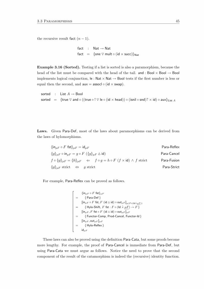
3.3 Paramorphisms 45
the recursive result fact (n− 1).
fact : Nat → Nat
fact = 〈|one Omult ◦ (id× succ)|〉Nat
Example 3.16 (Sorted). Testing if a list is sorted is also a paramorphism, because thehead of the list must be compared with the head of the tail. and : Bool × Bool → Bool
implements logical conjunction, le : Nat×Nat → Bool tests if the first number is less orequal then the second, and aux = assocl ◦ (id× swap).
sorted : List A → Bool
sorted = 〈|true O and ◦ ((true ◦ ! O le ◦ (id× head)) ◦ (isnil ◦ snd)?× id) ◦ aux|〉List A
Laws. Given Para-Def, most of the laws about paramorphisms can be derived fromthe laws of hylomorphisms.
〈|inµF ◦ F fst|〉µF = idµF Para-Reflex
〈|g|〉µF ◦ inµF = g ◦ F (〈|g|〉µF M id) Para-Cancel
f ◦ 〈|g|〉µF = 〈|h|〉µF ⇐ f ◦ g = h ◦ F (f × id) ∧ f strict Para-Fusion
〈|g|〉µF strict ⇔ g strict Para-Strict
For example, Para-Reflex can be proved as follows.
266666666666666664
〈|inµF ◦ F fst|〉µF
= {Para-Def }[[inµF ◦ F fst, F (id M id) ◦ outµF ]]µ(F◦(Id×µF ))
= {Hylo-Shift, F fst : F ◦ (Id × µF ).→ F }
[[inµF , F fst ◦ F (id M id) ◦ outµF ]]µF
= {Functor-Comp, Prod-Cancel, Functor-Id }[[inµF , outµF ]]µF
= {Hylo-Reflex }idµF
These laws can also be proved using the definition Para-Cata, but some proofs becomemore lengthy. For example, the proof of Para-Cancel is immediate from Para-Def, butusing Para-Cata we must argue as follows. Notice the need to prove that the secondcomponent of the result of the catamorphism is indeed the (recursive) identity function.

46 Chapter 3: Recursion Patterns as Hylomorphisms
26666666666666666666666666666666664
〈|g|〉 ◦ in
= {Para-Cata }fst ◦ (|g M in ◦ F snd|) ◦ in
= {Cata-Cancel }fst ◦ (g M in ◦ F snd) ◦ F (|g M in ◦ F snd|)
= {Prod-Cancel, Prod-Reflex }g ◦ F ((fst M snd) ◦ (|g M in ◦ F snd|))
= {Prod-Fusion, Para-Cata }g ◦ F (〈|g|〉 M snd ◦ (|g M in ◦ F snd|))
= {Prod-Fusion }264 snd ◦ (g M in ◦ F snd)
= {Prod-Cancel }in ◦ F snd
g ◦ F (〈|g|〉 M (|in|))= {Cata-Reflex }
g ◦ F (〈|g|〉 M id)
The uniqueness law for paramorphisms is specified as follows.
f = 〈|g|〉µF ∧ g strict ⇔ f ◦ inµF = g ◦ F (f M id) ∧ f strict Para-Uniq
Unfortunately this law cannot be derived from the previous ones, as was the case withcatamorphisms and anamorphisms. Instead we must resort to the original proof byMeertens [Mee92], based on the definition Para-Cata and the uniqueness of catamor-phisms. The proof of the ⇒ implication is the same of Para-Cancel stated above. Theother implication can be proved as follows.
2666666666666666666666666666666666666664
f
= {Prod-Cancel }fst ◦ (f M id)
= {Cata-Uniq, Prod-Strict, f strict, id strict }26666666666666666666664
(f M id) ◦ in
= {Prod-Fusion }f ◦ in M in
= { f ◦ in = g ◦ F (f M id) }g ◦ F (f M id) M in
= {Functor-Id }g ◦ F (f M id) M in ◦ F id
= {Prod-Cancel }g ◦ F (f M id) M in ◦ F snd ◦ F (f M id)
= {Prod-Fusion }(g M in ◦ F snd) ◦ F (f M id)
fst ◦ (|g M in ◦ F snd|)= {Para-Cata }
〈|g|〉
Meertens’ original proof did not include the strictness side conditions. Essentially,

3.3 Paramorphisms 47
these are equivalent to Para-Strict, which can be proved as follows.
2666666666664
g strict
⇒ { In-Strict, Snd-Strict, Strict-Comp, Prod-Strict }g M in ◦ F snd strict
⇒ {Cata-Strict }(|g M in ◦ F snd|) strict
⇒ {Fst-Strict, Strict-Comp, Para-Cata }〈|g|〉 strict
2666666666664
〈|g|〉 strict
⇒ { In-Strict, Strict-Comp }〈|g|〉 ◦ in strict
⇒ {Para-Cancel }g ◦ F (〈|g|〉 M id) strict
⇒ {Comp-Strict }g strict
Since the definition using a hylomorphism satisfies Para-Cancel, by uniqueness bothdefinitions are equal, at least for strict parameters.
Expressiveness. Since the expressive power of paramorphisms is greater than that ofcatamorphisms, it is possible to express the latter using the former.
(|g|)µF = 〈|g ◦ F fst|〉µF Cata-Para
The proof is similar to that of Para-Reflex.
266666666666666664
〈|g ◦ F fst|〉µF
= {Para-Def }[[g ◦ F fst, F (id M id) ◦ outµF ]]µ(F◦(Id×µF ))
= {Hylo-Shift, F fst : F ◦ (Id × µF ).→ F }
[[g, F fst ◦ F (id M id) ◦ outµF ]]µF
= {Functor-Comp, Prod-Cancel, Functor-Id }[[g, outµF ]]µF
= {Cata-Def }(|g|)µF
As a final remark, it can be proved that any function of the appropriate type can bedefined as a paramorphism.
g = 〈|g ◦ inµF ◦ F snd|〉µF
As the proof shows, this result is only of theoretical interest. Notice that the resultingfunction is not even recursive.
2666666666664
〈|g ◦ inµF ◦ F snd|〉µF
= {Para-Cancel, In-Out-Iso }g ◦ inµF ◦ F snd ◦ F (〈|g ◦ inµF ◦ F snd|〉µF M id) ◦ outµF
= {Functor-Comp, Prod-Cancel }g ◦ inµF ◦ F id ◦ outµF
= {Functor-Id, In-Out-Iso }g

48 Chapter 3: Recursion Patterns as Hylomorphisms
3.4 Apomorphisms
The apomorphism is the dual recursion pattern of the paramorphism, and therefore itcan express functions defined by primitive corecursion. Apomorphisms were introducedindependently by Vene and Uustalu [VU98] and Vos [Vos95]. While in an anamorphismthe coalgebra determines the arguments of the recursive calls, the parameter of anapomorphism can also be used to determine directly the result without recursion. Forexample, for naturals this recursion pattern can be encoded in Haskell as follows.
apo_Nat :: (a -> Maybe (Either a Nat)) -> a -> Nat
apo_Nat h a = case h a of Nothing -> Zero
Just (Left b) -> Succ (apo_Nat h b)
Just (Right n) -> Succ n
Definition. Given a function h : A → F (A + µF ), an apomorphism bd〈h〉ce can bedefined generically using a hylomorphism.
bd〈h〉ceµF : A → µF
bd〈h〉ceµF = [[inµF ◦ F (id O id), h]]µ(F◦(Id+µF ))
Apo-Def
The typing information is summarized in the following diagram.
A
bd〈h〉ceµF
��
h // F (A + µF )
F (bd〈h〉ceµF +id)
��µF F (µF )
inµF
oo F (µF + µF )F (idOid)
oo
Dually to paramorphisms, apomorphisms were initially defined using anamorphismsand sums [VU98].
bd〈h〉ceµF = bd(h O F inr ◦ outµF )ceµF ◦ inl Apo-Ana
Example 3.17 (Plus). Using apomorphisms a more natural definition of plus can begiven. Unlike the definition using anamorphisms (presented in Example 3.13), whereboth arguments were fully traversed recursively, with apomorphisms one of the argu-ments can be immediately returned when the other reaches zero. The implementationusing apo Nat is
plus :: (Nat, Nat) -> Nat
plus = apo_Nat h
where h (Zero, Zero) = Nothing
h (Succ n, Zero) = Just (Right n)
h (n, Succ m) = Just (Left (n,m))

3.4 Apomorphisms 49
In the point-free style it can be defined as follows. Some extra work is needed in orderto simulate the non disjunct pattern matching.
plus : Nat× Nat → Nat
plus = bd〈(id + coswap) ◦ coassocr ◦ (fst + in× id) ◦ distr ◦ (out× out)〉ceNat
Example 3.18 (Snoc). Appending an element to the end of a list can also be imple-mented as an apomorphism. When the end of the list is reached, the singleton list withthe element is returned.
snoc : A× List A → List A
snoc = bd〈inr ◦ undistr ◦ coswap ◦ (id× nil + aux) ◦ distr ◦ (id× out)〉ceList A
This definition uses the following auxiliary rearranging function.
aux : A× (B × C) → B × (A× C)aux = assocr ◦ (swap× id) ◦ assocl
Example 3.19 (Insert). Another good example of an apomorphism is the functionthat inserts an element in an ordered list, since when the correct place is found thefunction can return immediately.
insert : A× List A → List A
insert = bd〈inr ◦ undistr ◦ (inr O (inr O inl)) ◦ aux ◦ distr ◦ (id× out)〉ceList A
The definition of the auxiliary function is quite complex, mainly due to the need torearrange values.
aux = id× nil + ((id× cons) ◦ assocr + assocr ◦ (swap× id)) ◦ distl ◦ (le?× id) ◦ assocl
Laws. From the definition Apo-Def the following laws can be easily derived. They canalso be derived from Apo-Ana with some additional work.
bd〈F inl ◦ outµF 〉ce = idµF Apo-Reflex
outµF ◦ bd〈h〉ceµF = F (bd〈h〉ceµF O id) ◦ h Apo-Cancel
bd〈f〉ceµF ◦ g = bd〈h〉ceµF ⇐ f ◦ g = F (g + id) ◦ h Apo-Fusion
bd〈h〉ceµF strict ⇐ h strict Apo-Strict
The uniqueness law for apomorphisms is specified as follows.
f = bd〈h〉ceµF ⇔ outµF ◦ f = F (f O id) ◦ h Apo-Uniq

50 Chapter 3: Recursion Patterns as Hylomorphisms
Likewise to paramorphisms, a direct proof of uniqueness cannot be given using def-inition Apo-Def and the basic hylomorphism laws. Instead, definition Apo-Ana and theuniqueness law of anamorphisms must be used. The proof is similar to that of paramor-phisms and will be omitted (see [VU98] for details). Since Apo-Cancel follows fromApo-Def, by uniqueness this definition is equivalent to Apo-Ana.
Expressiveness. The fact that apomorphisms are at least as expressive as anamor-phisms is clear in the following law.
bd(h)ceµF = bd〈F inl ◦ h〉ceµF Ana-Apo
Finally, similarly to paramorphisms, it can be proved that any function of the ap-propriate type can be defined as an apomorphism.
h = bd〈F inr ◦ outµF ◦ h〉ceµF
3.5 Accumulations
Accumulations are binary functions that use the second parameter to store intermediateresults. The so called “accumulation technique” is typically used in functional program-ming to derive efficient implementations of some recursive functions. In the next chapterwe will present several examples of using this technique, but with accumulations definedin the curried style as higher order catamorphisms. Alberto Pardo defined (in the Set
category) a generic version of an uncurried accumulation recursion pattern, that can beused for any inductive data type [Par03].
This recursion pattern can be implemented in Haskell for the Nat data type as follows.Unlike the previous recursion patterns, this operator is parameterized by two functions.The first is used to combine the recursive result and the accumulating parameter inorder to produce the result. The second determines how the accumulator is modifiedbetween recursive calls.
accum_Nat :: ((Maybe a, b) -> a) -> (b -> b) -> (Nat, b) -> a
accum_Nat g t (Zero, x) = g (Nothing, x)
accum_Nat g t (Succ n, x) = g (Just (accum_Nat g t (n, t x)), x)
For example, plus can easily be implemented with this recursion operator, by treat-ing the second argument as an accumulating parameter. There are two possible im-plementations. The first does not take advantage of the accumulator, and uses it as aconstant parameter.
plus :: (Nat, Nat) -> Nat
plus = accum_Nat g id

3.5 Accumulations 51
where g (Nothing, x) = x
g (Just n, x) = Succ n
The second increments the accumulator while traversing the first argument, and essen-tially corresponds to a tail-recursive implementation of addition.
plus :: (Nat, Nat) -> Nat
plus = accum_Nat g Succ
where g (Nothing, x) = x
g (Just n, x) = n
Definition. This recursion pattern can be expressed as a hylomorphism using as in-termediate structure a labeled variant of the input data type – all nodes of the input aretagged with a value of the same type as the accumulating parameter. Assuming thatthis type is X, the labeled variant of µF can be obtained by µ(F ×X). For example,an accumulation over naturals uses the intermediate data type µ((1 + Id) ×X). If CPO
was distributive, this data type would be isomorphic to non-empty lists with elementsof type X.
Given g : FA×X → A, and τ : F (µF )×X → F (µF ×X), an accumulation {|g, τ |}can be defined generically as the following hylomorphism.
{|g, τ |}µF : µF ×X → A
{|g, τ |}µF = [[g, (τ M snd) ◦ (outµF × id)]]µ(F ×X)
Accum-Def
The typing information is depicted in the following diagram.
µF ×XoutµF×id
//
{|g,τ |}µF
��
F (µF )×XτMsnd// F (µF ×X)×X
F {|g,τ |}µF×id
��A F A×Xg
oo
As can be seen in this definition, τ is the function responsible for propagating theaccumulator to the recursive calls. This function should be proper for accumulation,that is, it should be a natural transformation of type
τ : F ×X.→ F ◦ (Id ×X) Tau-Nat
which guarantees that the propagated accumulation does not depend on the recursivevalues of the data type. τ also cannot modify the shape of the data type, or the datacontained in it, as captured by the following restriction.
F fst ◦ τ = fst Tau-Cancel

52 Chapter 3: Recursion Patterns as Hylomorphisms
As shown in [Par00], this recursion pattern can also be defined in curried form asa higher-order catamorphism, that is, one that returns a value of functional type. Torecover the expected type this catamorphism must be uncurried. According to Exp-Uniq,that can be done by wrapping it with ap ◦ (· × id). The resulting definition is
{|g, τ |}µF = ap ◦ ((|g ◦ (F ap ◦ τ M snd)|)µF × id) Accum-Cata
Although rather incomprehensible, this alternative definition is useful to prove theuniqueness law, and can be proved equivalent to Accum-Def.
Example 3.20 (Plus). As seen above, plus is one of the simplest examples of definitionsthrough accumulation. For naturals, in order for τ to be proper for accumulation, itshould have shape fst + id× φ, where φ : X → X. This is the reason why in the aboveHaskell implementation a function of this type was required as parameter. The tailrecursive plus can be defined as follows.
plus : Nat× Nat → Nat
plus = {|(snd O fst) ◦ distl, (fst + id× succ) ◦ distl|}Nat
Example 3.21 (Reverse). It is possible to define an efficient tail recursive reverse func-tion using accumulations. While traversing the input list, the current element is addedat the head of the accumulator. For lists, in order for τ to be proper for accumulation,it should have shape (fst+assocr◦ (fstMφ◦ (fst× id)))◦distl, where φ : A×X → X. Thislast function reflects the fact that the new value of the accumulator can only dependon the head of the list and on its own current value. In the reverse function φ will beinstantiated with cons. The accumulation is encoded in the following auxiliary function.
aux = {|(snd O snd ◦ fst) ◦ distl, (fst + assocr ◦ (fst M cons ◦ (fst× id))) ◦ distl|}List A
The reverse function just needs to initialize the accumulator with the empty list.
reverse : List A → List A
reverse = aux ◦ (id M nil ◦ !)
Laws. Again, most of the laws about generic accumulations can be derived from thedefinition as a hylomorphism. For example, the reflexivity law is defined and proved asfollows.
{|inµF ◦ fst, τ |}µF = fst Accum-Reflex

3.5 Accumulations 53
26666666666666666666666666666666664
{|inµF ◦ fst, τ |}µF
= {Accum-Def }[[inµF ◦ fst, (τ M snd) ◦ (outµF × id)]]µ(F ×X)
= {Hylo-Shift, fst : F ×X.→ F }
[[inµF , fst ◦ (τ M snd) ◦ (outµF × id)]]µF
= {Prod-Cancel }[[inµF , τ ◦ (outµF × id)]]µF
= {Hylo-Fusion }26666664F fst ◦ τ ◦ (outµF × id)
= {Tau-Cancel }fst ◦ (outµF × id)
= {Prod-Def, Prod-Cancel }outµF ◦ fst
[[inµF , outµF ]]µF ◦ fst
= {Hylo-Reflex }fst
The following can also be easily proved.
{|g, τ |}µF ◦ (inµF × id) = g ◦ (F {|g, τ |}µF ◦ τ M snd) Accum-Cancel
f ◦ {|g, τ |}µF = {|h, τ |}µF ⇐ f ◦ g = h ◦ (F f × id) ∧ f strict Accum-Fusion
As expected, these laws can also be proved using the definition Accum-Cata. Forexample, Accum-Cancel can be proved as follows.
2666666666666666666666666664
{|g, τ |} ◦ (in× id)
= {Accum-Cata, Prod-Functor-Comp }ap ◦ ((|g ◦ (F ap ◦ τ M snd)|) ◦ in× id)
= {Cata-Cancel, Prod-Functor-Comp }ap ◦ (g ◦ (F ap ◦ τ M snd)× id) ◦ (F (|g ◦ (F ap ◦ τ M snd)|)× id)
= {Exp-Cancel }g ◦ (F ap ◦ τ M snd) ◦ (F (|g ◦ (F ap ◦ τ M snd)|)× id)
= {Prod-Fusion, Prod-Cancel }g ◦ (F ap ◦ τ ◦ (F (|g ◦ (F ap ◦ τ M snd)|)× id) M snd)
= {Tau-Nat }g ◦ (F ap ◦ F ((|g ◦ (F ap ◦ τ M snd)|)× id) ◦ τ M snd)
= {Functor-Comp, Accum-Cata }g ◦ (F {|g, τ |} ◦ τ M snd)
For this recursion pattern it is more interesting to study left-strictness, because therecursive parameter is the left element of the input pair. The following result holds.
{|g, τ |}µF , τ left-strict ⇔ g, τ left-strict Accum-Strict
Since this law is needed to prove uniqueness, the following proof is based on definitionAccum-Cata.

54 Chapter 3: Recursion Patterns as Hylomorphisms
26666666666666666666666666666666666664
g left-strict
⇒ { Lstrict-Def }g ◦ (⊥× id) = ⊥ ◦ fst
⇒ {Ap-Lstrict, Lstrict-Strict }g ◦ (F ap ◦ ⊥ × id) = ⊥ ◦ fst
⇒ {Prod-Def, τ left-strict }g ◦ (F ap ◦ τ ◦ (⊥× id) M snd) = ⊥ ◦ fst
⇒ {Prod-Cancel, Prod-Fusion }g ◦ (F ap ◦ τ M snd) ◦ (⊥× id) = ⊥ ◦ fst
⇒ { Lstrict-Def, Exp-Strict }g ◦ (F ap ◦ τ M snd) strict
⇒ {Cata-Strict }(|g ◦ (F ap ◦ τ M snd)|) strict
⇒ { Lstrict-Comp-Left, Ap-Lstrict }ap ◦ ((|g ◦ (F ap ◦ τ M snd)|)× id) left-strict
⇒ {Accum-Cata }{|g, τ |} left-strict
266666666666666666666666666666664
{|g, τ |} left-strict
⇒ { In-Strict, Lstrict-Comp-Left }{|g, τ |} left-strict ◦ (in× id)
⇒ {Accum-Cancel }g ◦ (F {|g, τ |} ◦ τ M snd) left-strict
⇒ { Lstrict-Def, Prod-Fusion }g ◦ (F {|g, τ |} ◦ τ ◦ (⊥× id) M snd ◦ (⊥× id)) = ⊥ ◦ fst
⇒ {Prod-Cancel, τ left-strict }g ◦ (F {|g, τ |} ◦ ⊥ ◦ fst M snd) = ⊥ ◦ fst
⇒ {Prod-Def, Prod-Functor-Comp }g ◦ (F {|g, τ |} × id) ◦ (⊥× id) = ⊥ ◦ fst
⇒ { Lstrict-Def }g ◦ (F {|g, τ |} × id) left-strict
⇒ {Comp-Lstrict }g left-strict
In practice, verifying these strictness conditions is easy. As seen in the examples,most parameters of accumulations are of the form (·O ·) ◦ distl. By definition any eitheris strict, and distl is a left-strict function, which by Lstrict-Comp-Right leads necessarilyto a left-strict parameter.
The uniqueness law for accumulations is specified as follows.
f = {|g, τ |}µF ∧ g, τ left-strict⇔
f ◦ (inµF × id) = g ◦ (Ff ◦ τ M snd) ∧ f, τ left-strict
Accum-Uniq
Similarly to paramorphisms, this law can be proved using the definition Accum-Cata.However, since accumulations defined using Accum-Def also satisfy Accum-Cancel, bothdefinitions are equivalent provided that both g and τ are left-strict. The implication⇒ and the strictness side conditions are equivalent, respectively, to Accum-Cancel andAccum-Strict, already proved using that definition. For the⇐ implication the uniquenesslaw of catamorphisms is used, as shown in the following calculation.

3.5 Accumulations 55
266666666666666666666666666666666666666666664
f
= {Exp-Cancel }ap ◦ (f × id)
= {Cata-Uniq, Exp-Strict, f left-strict }2666666666666666666666666664
f ◦ inµF
= {Exp-Fusion }f ◦ (inµF × id)
= { f ◦ (inµF × id) = g ◦ (F f ◦ τ M snd) }g ◦ (F f ◦ τ M snd)
= {Functor-Id, Exp-Cancel, Functor-Comp }g ◦ (F ap ◦ F (f × id) ◦ τ M snd)
= {Tau-Nat }g ◦ (F ap ◦ τ ◦ (F f × id) M snd)
= {Prod-Cancel, Prod-Def }g ◦ (F ap ◦ τ ◦ (F f × id) M snd ◦ (F f × id))
= {Prod-Fusion, Exp-Fusion }g ◦ (F ap ◦ τ M snd) ◦ F f
ap ◦ ((|g ◦ (F ap ◦ τ M snd)|)× id)
= {Accum-Cata }{|g, τ |}
Besides Accum-Fusion, Pardo presents other specific fusion laws for this recursionpattern. For example, a change in the accumulating parameter, by means of a functionf : X → Y , can be fused in the following way.
{|g, τ |}µF ◦ (id× f) = {|g ◦ (id× f), φ|}µF ⇐ τ ◦ (id× f) = F (id× f) ◦ φ
The proof uses the definition Accum-Def.
2666666666666666666666666666666666666664
{|g, τ |}µF ◦ (id× f)
= {Accum-Def }[[g, (τ M snd) ◦ (outµF × id)]]µ(F ×Y ) ◦ (id× f)
= {Hylo-Fusion }266666666666666664
(τ M snd) ◦ (outµF × id) ◦ (id× f)
= {Prod-Functor-Comp }(τ M snd) ◦ (id× f) ◦ (outµF × id)
= {Prod-Fusion, Prod-Def, Prod-Cancel }(τ ◦ (id× f) M f ◦ snd) ◦ (outµF × id)
= { τ ◦ (id× f) = F (id× f) ◦ φ }(F (id× f) ◦ φ M f ◦ snd) ◦ (outµF × id)
= {Prod-Absor, Prod-Functor-Comp }(F (id× f)× id) ◦ (id× f) ◦ (φ M snd) ◦ (outµF × id)
[[g, (id× f) ◦ (φ M snd) ◦ (outµF × id)]]µ(F ×Y )
= {Hylo-Shift, id× f : F ×X.→ F × Y }
[[g ◦ (id× f), (φ M snd) ◦ (outµF × id)]]µ(F ×X)
= {Accum-Def }{|g ◦ (id× f), φ|}µF

56 Chapter 3: Recursion Patterns as Hylomorphisms
3.6 Summary
In this chapter we have shown how to define some typical recursion patterns usinghylomorphisms. This approach has several advantages:
• It avoid proofs by fixpoint induction – all the usual properties of the recursionoperators, including uniqueness, can be proved either using just a small set of lawsabout hylomorphisms, or previously derived laws about other recursion operators.
• It increases the understanding of the recursion patterns – for the more advancedoperators, the definition using hylomorphisms is more understandable than theoriginal one using other recursion patterns. This is the case of paramorphisms andaccumulations, where the original definition using catamorphisms can be difficultto understand.
• It also systematizes the proof of the strictness side conditions that characterizeinitial recursion patterns in CPO – these can also be derived by calculation fromsimple laws concerning the strictness of hylomorphisms and of the basic combina-tors. To our knowledge, this is also the first time that the strictness side conditionsassociated with generic accumulations are precisely stated.
The same technique can be applied to other recursion patterns. For example, his-tomorphisms and generalized catamorphisms can also be defined using hylomorphisms.The histomorphism recursion pattern (together with its dual – futumorphisms) was firstpresented in [UV99]. It generalizes catamorphisms by allowing the result to depend notonly on the recursive result of applying the function to the immediate children of theinput, but also on the recursive result of any subterm. For example, it can be used todefine the Fibonacci function that, for a given n, depends on the value of applying itto n− 1 and n− 2. The generalized catamorphisms is a “meta recursion pattern”, firstpresented in [UVP01], that is parameterized by a comonad that encodes the recursivecall pattern of a specific recursion pattern. By changing the comonad, it can be used todefine catamorphisms, paramorphisms, or histomorphisms.

Chapter 4
Calculating Accumulations Using
Fusion
The main goal of this chapter is to revisit some classic work in the area of programtransformation using pure point-free calculations. The chapter is focused on the trans-formation of programs by introducing new accumulating parameters, according to thestrategy initially proposed by Bird [Bir84], where the transformed programs are seenas higher-order folds calculated systematically from a specification. We present a sys-tematic approach to this program transformation technique, together with a substantialnumber of examples. This systematization leads to a set of generic transformationschemes, that can be used as shortcut optimization rules in an automatic programtransformation system.
Another goal is the improvement of the machinery that is used to perform point-freecalculations in a higher-order setting. Quoting Jeremy Gibbons [Gib94],
We are interested in extending what can be calculated precisely becausewe are not interested in the calculations themselves [. . . ]
In other words, we aim at extending the calculus with new useful operators that helpreduce the burden of proofs just to the creative parts.
4.1 A Motivating Example
Consider the reverse function on lists. Obtaining the accumulator-based linear timeversion of this function from the single-argument quadratic time version is a classicexample of a program transformation.
In this section this example will be used to briefly review different transformationtechniques for optimizing programs by introducing accumulating parameters. As seenin Section 3.5, the resulting functions are called accumulations. However, the accumula-tions derived here are quite different from the ones presented in that section, since they
57

58 Chapter 4: Calculating Accumulations Using Fusion
are in the curried form – the input data-structure is traversed using a catamorphism,that outputs a function to be later applied to the accumulating parameter.
4.1.1 Transformation With Fold/Unfold Rules
Consider the typical definition of reverse in Haskell.
reverse :: List a -> List a
reverse Nil = Nil
reverse (Cons h t) = cat (reverse t, Cons h Nil)
In order to apply a fold/unfold rule-based transformation [BD77, PP96] we will startwith an equivalent definition using conditionals. The abbreviation wrap h = cons (h, nil)will also be used. To simplify the presentation, when working in the pointwise style nil
will denote the empty list (the exact definition is nil ⊥1).
reverse l = if (isnil l) then nil
else (cat (reverse (tail l),wrap (head l)))
The transformation steps should be oriented by the so-called forced folding (or need-for-folding) principle [Dar81], which states that after the unfold step, the program shouldbe manipulated so that a folding step can be applied to a different sub-expression.Hopefully these manipulations will lead to improvements at all levels of the recursiontree. We can try to apply this strategy directly to the above definition.26666666666666666666666666666666664
reverse l
= {definition of reverse }if (isnil l) then nil
else (cat (reverse (tail l), wrap (head l)))
= {unfold }if (isnil l) then nil
else (cat (if (isnil (tail l)) then nil
else (cat (reverse (tail (tail l)), wrap (head (tail l)))), wrap (head l)))
= {distributing of cat over the conditional }if (isnil l) then nil
else (if (isnil (tail l)) then (cat (nil, wrap (head l)))
else (cat (cat (reverse (tail (tail l)), wrap (head (tail l)))), wrap (head l)))
= { associativity of cat }if (isnil l) then nil
else (if (isnil (tail l)) then (cat (nil, wrap (head l)))
else (cat (reverse (tail (tail l)), cat(wrap (head (tail l)), wrap (head l)))))
At this point one would like to be able to fold the expression using the definitionof reverse; however, the presence of the expression wrap (head l) in both cases of theconditional prevents this step. We must appeal to the generalization strategy [BD77],according to which a new function definition is introduced.

4.1 A Motivating Example 59
aux (l, y) = cat (reverse l, y)
This definition can indeed be transformed until a fold step is performed.266666666666666666666666666666664
aux (l, y)
= {definition of aux }cat (reverse l, y)
= {unfold }cat (if (isnil l) then nil
else (cat (reverse (tail l), wrap (head l))), y)
= {distributing cat over the conditional }if (isnil l) then (cat (nil, y))
else (cat (cat (reverse (tail l), wrap (head l))), y)
= { associativity of cat }if (isnil l) then (cat (nil, y))
else (cat (reverse (tail l), cat (wrap (head l), y)))
= { fold }if (isnil l) then (cat (nil, y))
else (aux (tail l, cat (wrap (head l), y)))
The definition of cat can be used to simplify the resulting expression, yielding thedefinition
aux (l, y) = if (isnil l) then y else (aux (tail l, cons (head l, y)))
Finally, since cat has a right-identity we have26666664reverse l
= { right-identity of cat }cat (reverse l, nil)
= {definition of aux }aux (l, nil)
The definition of aux, together with this last equation, is the final result of thetransformation. In Haskell one would write
reverse :: List a -> List a
reverse l = aux (l, Nil)
aux :: (List a, List a) -> List a
aux (Nil, y) = y
aux (Cons h t, y) = aux (t, Cons h y)
Remark. Notice that the transformed program is tail-recursive, i.e. the result of therecursive call is passed directly as the result of the invoking call. Linear tail-recursivefunctions can be converted into iterative code (i.e. with recursion totally removed)using a straightforward transformation scheme. Removal of recursion is a major goal

60 Chapter 4: Calculating Accumulations Using Fusion
of program transformation, even when it can be only partially achieved, as is the casewith functions over trees. In Section 4.2.3 it will be seen, for the case of binary trees,that only one of the two recursive calls is made tail-recursive.
The asymptotic improvement in the execution time is a somewhat casual side-effectof the transformation – it is a consequence of the associativity property of the appendoperator, and the fact that it runs in linear time on the size of its first argument. InSection 4.2.1 we consider the transformation of the function which calculates the productof the numbers in a list. Since arithmetic product is calculated in constant time, thistransformation does not change the asymptotic execution time; however, it still is auseful transformation since it produces a tail-recursive definition.
4.1.2 Transformation by Calculation
The first application of the calculational approach to program transformation, as popu-larized by Richard Bird and Lambert Meertens in the mid-80s, was precisely the deriva-tion of functions with accumulations from inefficient specifications [Bir84]. In this sem-inal paper, Bird introduced the fundamental idea behind this transformation method:first the recursive functions are specified using a standard recursion pattern; then fusionis used together with the generalization strategy (as used in fold/unfold transforma-tion), in order to derive a hopefully more efficient implementation with an accumulatingparameter. We remark that fusion was then called promotion and the fold recursionpattern had not yet been isolated in a higher-order operator such as foldr.
The functions resulting from such transformations have two arguments (the secondof which is the accumulator). In order to be able to write them using the fold recursionpattern, Bird resorted to currying: accumulations are written as higher-order folds,returning a function as result. Apart from some refinements in the basic laws andnotation, this technique was later used by several authors [MFP91, HIT99, dMS99,SdM03]. However, none of these works presents these calculations in pure point-freestyle. Moreover, some of them don’t use the generic fusion law for catamorphismspresented in Section 3.1. Instead, they use the pointwise specialization of this law forparticular data types, such as the following one for the curried foldr operator defined onlists (with type (A → B → B) → B → List A → B).
f (foldr g e l) = foldr h c l
⇐f strict ∧ f e = c ∧ ∀x, r · f (g x r) = h x (f r)
Turning now to our running example, we will start from where the application of thegeneralization strategy led us in the previous section (except that the new function isin curried style). Notice that, in the remaining of the chapter the name ft will be used

4.1 A Motivating Example 61
to denote the accumulation obtained by transforming f .
reverset l y = cat (reverse l) y
Following the approach just described, in order to obtain the desired accumulationthe concatenation operator must be fused with the reverse function, using the above law.For that, it is necessary to redefine reverse using the foldr operator.
reverse : List A → List A
reverse = foldr (λxr. cat r (wrap x)) nil
Dropping the accumulating parameter from our specification we get
reverset l = cat (foldr (λxr. cat r (wrap x)) nil l)
This is a suitable expression to apply fusion, with f instantiated to cat, the curriedversion of the concatenation operator. Notice that, since cat is left-strict, cat is a strictfunction due to Exp-Strict. In order to apply fusion there still remains two premises toverify, which will in turn allow us to determine c and h.
cat nil = c
λxr. cat (cat r (wrap x)) = λxr. h x (cat r)
Notice the use of λ-abstraction to encode universal quantification.
Since nil is also a left-identity of concatenation, then c = id. In order to determineh the calculation proceeds as follows.
λxr. cat (cat r (wrap x))= { η-expansion }
λxr.λy. cat (cat r (wrap x)) y
= { associativity of cat }λxr.λy. cat r (cat (wrap x) y)
= {definitions of cat, wrap }λxr.λy. cat r (cons (x, y))
It is now fairly clear that h can be defined as
h x z = λy. z (cons (x, y))

62 Chapter 4: Calculating Accumulations Using Fusion
The result of applying the fusion law is thus the following higher-order fold.
reverset : List A → List A → List A
reverset = foldr (λxzy. z (cons (x, y))) id
After expanding the definition of foldr we get the curried version of the aux function cal-culated in the previous section. It should be invoked as reverse l = reverse_t l Nil.
reverse_t :: List a -> List a -> List a
reverse_t Nil y = y
reverse_t (Cons h t) y = reverse_t t (Cons h y)
To sum up, the creative step involved in this technique is exactly the same as whenusing fold/unfold transformations – writing the specification corresponds to using thegeneralization strategy. However, for the particular technique of accumulations, anyexperienced functional programmer should have no problem in writing them directly. Amajor advantage of the calculational approach is that, by structuring recursion in fixedpatterns, it is possible, as will be largely exemplified in this chapter, to define laws thatcombine in a single shortcut step whole sequences of transformation steps.
4.1.3 Transformation in the Point-free Style
The third method, which will be used extensively in the remaining of the chapter, differsfrom the one presented above in that all the calculations are done in point-free. Beforethis can be done, the initial specification needs to be written in the point-free style. Thereverse function can be defined as
reverse : List A → List A
reverse = (|nil O cat ◦ swap ◦ (wrap× id)|)List A
and the specification asreverset = cat ◦ reverse
The derivation will be based on the generic fusion law Cata-Fusion. According tothis law (and since cat is strict), in order to obtain the desired definition of reverset,which is a catamorphism (|h|), we must find a function h such that
cat ◦ (nil O cat ◦ swap ◦ (wrap× id)) = h ◦ FList cat = h ◦ (id + id× cat)
In both fold/unfold and the pointwise calculational transformations seen in the pre-vious sections, one of the major steps was the application of the associativity propertyof cat (this is in general the case for all transformations involving accumulations). Sothe question arises of how to express this property in the point-free style.

4.1 A Motivating Example 63
Consider an arbitrary operator ⊕. One possibility for expressing its associativity isto use the equation
⊕ ◦ (id×⊕) ◦ assocr = ⊕ ◦ (⊕× id)
This formulation is not very practical because the operator which will be fused is incurried form. As such, it is desirable to introduce new combinators particularly tailoredto express properties in a higher-order setting. For the particular case of associativity,it suffices to introduce an uncurried composition operator.
comp (f, g) = f ◦ g
In the point-free style it can be defined using the exponential combinators.
comp : (CB ×BA) → CA
comp = ap ◦ (id× ap) ◦ assocrComp-Def
To show that this point-free definition implements the behavior specified in pointwise,the following fact can be proved.
comp ◦ (f M g) = f ◦ g Comp-Pnt
26666666666666666666666666666666666664
comp ◦ (f M g)
= {Comp-Def, Exp-Fusion }ap ◦ (id× ap) ◦ assocr ◦ ((f M g)× id)
= {Prod-Absor, Prod-Functor-Comp, Assocr-Nat }ap ◦ (id× ap) ◦ (f × (g × id)) ◦ assocr ◦ ((id M id)× id)
= {Prod-Functor-Comp, Pnt-Def }ap ◦ (f ◦ snd× id) ◦ (id× ap ◦ (g ◦ snd× id)) ◦ assocr ◦ ((id M id)× id)
= {Exp-Cancel }f ◦ snd ◦ (id× g ◦ snd) ◦ assocr ◦ ((id M id)× id)
= {Prod-Def, Prod-Cancel, Assocr-Def }f ◦ g ◦ snd ◦ snd ◦ (fst ◦ fst M (snd× id)) ◦ ((id M id)× id)
= {Prod-Cancel, Prod-Functor-Comp }f ◦ g ◦ snd ◦ (snd ◦ (id M id)× id)
= {Prod-Def, Prod-Cancel }f ◦ g ◦ snd
= {Pnt-Def }f ◦ g
Using this combinator, associativity of ⊕ can be expressed more usefully by equation
⊕ ◦ ⊕ = comp ◦ (⊕×⊕)
The following calculation shows that the latter formulation is a consequence of theformer.

64 Chapter 4: Calculating Accumulations Using Fusion
26666666666666666666666666666666666664
@ ⊕ ◦ (id×⊕) ◦ assocr = ⊕ ◦ (⊕× id)
⊕ ◦ ⊕= {Exp-Fusion }
⊕ ◦ (⊕× id)
= {@ }⊕ ◦ (id×⊕) ◦ assocr
= {Exp-Cancel, Prod-Functor-Comp }ap ◦ (⊕× id) ◦ (id× ap) ◦ (id× (⊕× id)) ◦ assocr
= {Prod-Functor-Comp }ap ◦ (id× ap) ◦ (⊕× (⊕× id)) ◦ assocr
= {Assocr-Nat }ap ◦ (id× ap) ◦ assocr ◦ ((⊕×⊕)× id)
= {Exp-Fusion }ap ◦ (id× ap) ◦ assocr ◦ (⊕×⊕)
= {Comp-Def }comp ◦ (⊕×⊕)
Equipped with this formulation of associativity, calculating the accumulation be-comes very simple.
26666666666666666666666666666666666664
@ cat ◦ cat = comp ◦ (cat× cat)
† cat ◦ nil = id
‡ cat ◦ wrap = cons
cat ◦ (nil O cat ◦ swap ◦ (wrap× id))
= {Sum-Fusion }cat ◦ nil O cat ◦ cat ◦ swap ◦ (wrap× id)
= { † }id O cat ◦ cat ◦ swap ◦ (wrap× id)
= {@ }id O comp ◦ (cat× cat) ◦ swap ◦ (wrap× id)
= {Swap-Nat, Prod-Functor-Comp }id O comp ◦ swap ◦ (cat ◦ wrap× cat)
= { ‡, Prod-Functor-Comp }id O comp ◦ swap ◦ (cons× id) ◦ (id× cat)
= {Sum-Absor }(id O comp ◦ swap ◦ (cons× id)) ◦ (id + id× cat)
The result of the transformation is thus
reverset : List A → (List A → List A)reverset = (|id O comp ◦ swap ◦ (cons× id)|)List A
To see that this is the expected point-free definition of reverset, it can be converted backto pointwise with the following calculation.

4.1 A Motivating Example 65
2666666666666666666666666664
reverset = (|id O comp ◦ swap ◦ (cons× id)|)List A
= {Cata-Cancel }reverset ◦ inList = (id O comp ◦ swap ◦ (cons× id)) ◦ FList reverset
= {definitions of FList and inList }reverset ◦ (nil O cons) = (id O comp ◦ swap ◦ (cons× id)) ◦ (id + id× reverset)
= {Sum-Fusion, Sum-Absor, Prod-Functor-Comp }reverset ◦ nil O reverset ◦ cons = id O comp ◦ swap ◦ (cons× reverset)
= {Sum-Equal }reverset ◦ nil = id ∧ reverset ◦ cons = comp ◦ swap ◦ (cons× reverset)
= { η-expansion, definitions of the basic combinators }reverset nil = id ∧ reverset (cons (x, xs)) = (reverset xs) ◦ (cons x)
= { η-expansion, definitions of the basic combinators }reverset nil y = id y ∧ reverset (cons (x, xs)) y = reverset xs (cons (x, y))
Remark. In this example, the solution to the premises of the Cata-Fusion law is notunique, as the following calculation shows.2666666666666666666666666664
† cat ◦ nil = id
cat ◦ (nil O cat ◦ swap ◦ (wrap× id))
= {Sum-Fusion }cat ◦ nil O cat ◦ cat ◦ swap ◦ (wrap× id)
= { † }id O cat ◦ cat ◦ swap ◦ (wrap× id)
= {Exp-Cancel }id O cat ◦ ap ◦ (cat × id) ◦ swap ◦ (wrap× id)
= {Swap-Nat, Prod-Functor-Comp }id O cat ◦ ap ◦ swap ◦ (wrap× cat)
= {Prod-Functor-Comp, Sum-Absor }(id O cat ◦ ap ◦ swap ◦ (wrap× id)) ◦ (id + id× cat)
This leads to the following definition of the accumulation.
reverset : List A → (List A → List A)reverset = (|id O cat ◦ ap ◦ swap ◦ (wrap× id)|)
After converting it into pointwise we would get.
reverse_t :: List a -> List a -> List a
reverse_t Nil y = y
reverse_t (Cons h t) y = cat (reverse_t t (wrap h), y)
This is of course a useless transformation – the resulting function runs in quadratictime and is not tail-recursive. This shows that some notion of a strategy is necessaryfor the calculations to be relevant for our goals. The distinctive feature of a usefultransformation in this particular case is its use of the associativity property of append,not used in the latter transformation.

66 Chapter 4: Calculating Accumulations Using Fusion
4.2 Calculating Accumulations in the Point-free Style
The methodology presented for deriving accumulations using the point-free style is stillnot very amenable for mechanization: the calculations require human intervention, notonly to decide which law to apply at each point, but also to identify a good target to guidethe derivation. As seen in the last remark, it is possible to derive accumulations that arenot “better” than the original functions. As such, in this section we will present a set oftransformation schemes, categorized by data type, whose derivation is performed onceand for all, and that guarantee the usefulness of the transformation. To apply thesetransformation schemes one has to prove very few side conditions (typically, just theassociativity of some operator), and thus could be used as shortcut optimization rulesin an automatic transformation system. The application of these rules is demonstratedin a substantial number of examples.
We start by presenting a transformation scheme that encapsulates the methodologyfor deriving accumulations in the calculational style using fusion. Among others, it ispresented also in [BdM97, HIT99], but is adapted here to the CPO setting. Given abinary operator ⊕ : A×B → B it is defined as follows.
(|f |)µF x = (|g|)µF x e
⇐⊕ ◦ f = g ◦ F ⊕ ∧ ⊕ (x, e) = x ∧ ⊕ left-strict
Cata-Accum
This scheme is too general to be useful, but will later be instantiated to more concreterules, to be applied in specific data types. In order to prove Cata-Accum, it should firstto converted into the point-free notation. The conclusion can be specified as
(|f |) = ap ◦ ((|g|) M e ◦ !)
Given that ⊕ has a right-identity e if ⊕◦ (idMe◦ !) = id, the calculation is rather trivial.
266666666666666666666666666664
† ⊕ ◦ (id M e ◦ !) = id
‡ ⊕ ◦ f = g ◦ F ⊕
(|f |)= { † }
⊕ ◦ (id M e ◦ !) ◦ (|f |)= {Prod-Fusion, Bang-Fusion }
⊕ ◦ ((|f |) M e ◦ !)
= {Exp-Cancel }ap ◦ (⊕× id) ◦ ((|f |) M e ◦ !)
= {Prod-Absor }ap ◦ (⊕ ◦ (|f |) M e ◦ !)
= {Cata-Fusion, ‡, Exp-Strict, ⊕ left-strict }ap ◦ ((|g|) M e ◦ !)

4.2 Calculating Accumulations in the Point-free Style 67
4.2.1 Tail-recursive Accumulations over Lists
Associative Operators. We start with the most classic example of applying theaccumulation strategy: to optimize the iteration of an associative operator over a list.Given a left-strict associative operator ⊕ : B×B → B with right identity e, an elementc : 1 → B, and a function f : A → B, it is possible to transform a function
h : List A → B
h = (|c O⊕ ◦ swap ◦ (f × id)|)List A
intoht : List A → B → B
ht = (|⊕ ◦ c O comp ◦ swap ◦ (⊕ ◦ f × id)|)List A
and replace every h l by ht l e.
This transformation is a consequence of Cata-Accum and the following calculation.2666666666666666666666666664
@ ⊕ ◦ ⊕ = comp ◦ (⊕×⊕)
⊕ ◦ (c O⊕ ◦ swap ◦ (f × id))
= {Sum-Fusion, ⊕ left-strict, Exp-Strict }⊕ ◦ c O⊕ ◦ ⊕ ◦ swap ◦ (f × id)
= {@ }⊕ ◦ c O comp ◦ (⊕×⊕) ◦ swap ◦ (f × id)
= {Swap-Nat }⊕ ◦ c O comp ◦ swap ◦ (⊕×⊕) ◦ (f × id)
= {Prod-Functor-Comp }⊕ ◦ c O comp ◦ swap ◦ (⊕ ◦ f ×⊕)
= {Prod-Functor-Comp, Sum-Absor }(⊕ ◦ c O comp ◦ swap ◦ (⊕ ◦ f × id)) ◦ (id + id×⊕)
In order to see what is going on, both functions can be translated into the pointwisestyle. It becomes clear that this transformation rule allows to convert the function
h nil = c
h (cons(x, xs)) = (h xs)⊕ (f x)
into the tail-recursive
ht nil y = c⊕ y
ht (cons(x, xs)) y = ht xs ((f x)⊕ y)
Example 4.1 (Reverse). It is immediate to see that the reverse function of Sec-tion 4.1.3 can be transformed using this rule, with the expected result.
Example 4.2 (Product). Suppose we want to derive a tail-recursive implementationof the following function that multiplies all the numbers in a list.

68 Chapter 4: Calculating Accumulations Using Fusion
product :: List Nat -> Nat
product Nil = Succ Zero
product (Cons h t) = mult (h, product t)
A straightforward implementation of this function in the point-free style is
product : List Nat → Nat
product = (|one Omult|)List Nat
The above transformation cannot be applied directly. However, since mult is a com-mutative operator and given Prod-Functor-Id, the above definition is equivalent to thefollowing.
product = (|one Omult ◦ swap ◦ (id× id)|)List Nat
Now, the transformation can be applied straightforwardly, resulting in the followingaccumulation (notice that as one is the unit of mult then mult ◦ one = id).
productt : List Nat → Nat → Nat
productt = (|id O comp ◦ swap ◦ (mult× id)|)List Nat
The final tail-recursive implementation in Haskell is
product :: List Nat -> Nat
product l = product_t l (Succ Zero)
product_t :: List Nat -> Nat -> Nat
product_t Nil y = y
product_t (Cons h t) y = product_t t (mult (h,y))
This example shows that it is not always immediate to apply the transformationrule to catamorphisms with associative operators. For many operators (namely forcommutative ones) the redefinition of the initial specification is trivial. The next examplepresents a situation where this is not so obvious.
Example 4.3 (Insertion Sort). Consider the insertion sort defined in Example 3.3
isort : List A → List A
isort = (|nil O insert|)List A
where the type of insert is A×List A → List A. This is clearly not an associative operator.In order to apply the transformation scheme, the definition has to be considerablymodified. First, notice that
insert = merge ◦ (wrap× id)

4.2 Calculating Accumulations in the Point-free Style 69
where merge is the (associative) merge function on sorted lists, which has the empty listas its right identity. Taking into account that merge is also commutative, insertion sortcan be redefined as follows.
isort = (|nil Omerge ◦ swap ◦ (wrap× id)|)List A
This definition is already suitable for the above transformation, with the result (no-tice that insert = merge ◦ wrap)
isortt : List A → List A → List A
isortt = (|id O comp ◦ swap ◦ (insert× id)|)List A
This means that insertion sort can be implemented as a tail-recursive definition.
isort :: (Ord a) => List a -> List a
isort l = isort_t l Nil
isort_t :: (Ord a) => List a -> List a -> List a
isort_t Nil y = y
isort_t (Cons h t) y = isort_t t (insert h y)
This example illustrates that the application of a transformation may require the intro-duction of new functions (as in the generalization strategy). These may eventually beeliminated after the shortcut is applied.
Operators With Associative Duals. The previous result can be generalized inorder to be applicable to a slightly more general class of programs. A binary operator⊕ is said to have an associative dual operator � [BW82] if
(x⊕ y)⊕ z = x⊕ (y � z)
In point-free notation the above equality can be written as
⊕ ◦ ⊕ = comp ◦ (⊕×�)
Given a left-strict operator ⊕ : B × C → B with right identity e and associativedual operator � : C × C → C, an element c : 1 → B, and a function f : A → C, then afunction
h : List A → B
h = (|c O⊕ ◦ swap ◦ (f × id)|)
can be transformed into
ht : List A → C → B
ht = (|⊕ ◦ c O comp ◦ swap ◦ (� ◦ f × id)|)

70 Chapter 4: Calculating Accumulations Using Fusion
by replacing every occurrence of h l by ht l e. The proof of this transformation rule issimilar to the previous one, because the associative dual law has a similar formulationto associativity.
Example 4.4 (Tree Sorts). Consider again the following definition of insertion sort,taken from Example 4.3.
isort = (|nil Omerge ◦ swap ◦ (wrap× id)|)List A
There is no reason which prevents an accumulator of a different type to be used,such as, a binary search tree. Instead of using a particular type of tree, lets assume theexistence of an abstract type Tree A, that comes equipped with the following functions.
treeToList : Tree A → List A
that produces the sorted list of the elements stored in the tree,
mkTree : A → Tree A
that generates a tree with a single element, and
mergeTree : Tree A× Tree A → Tree A
that merges two trees. The function that inserts an element in a tree can be defined asfollows.
insertTree : A× Tree A → Tree A
insertTree = mergeTree ◦ (mkTree× id)
In order to use trees as accumulators, we now simply try to rewrite the definition ofisort in such a way that wrap can be replaced by mkTree. The following calculation uses ashypothesis a property that we can reasonably expect to be verified by an implementationof trees. 266666666666666664
† treeToList ◦mkTree = wrap
merge ◦ swap ◦ (wrap× id)
= { † }merge ◦ swap ◦ (treeToList ◦mkTree× id)
= {Prod-Functor-Comp }merge ◦ swap ◦ (treeToList× id) ◦ (mkTree× id)
= {Swap-Nat }merge ◦ (id× treeToList) ◦ swap ◦ (mkTree× id)
By defining ⊕ = merge ◦ (id× treeToList) the sorting function can be defined as
sort = (|nil O⊕ ◦ swap ◦ (mkTree× id)|)List A

4.2 Calculating Accumulations in the Point-free Style 71
Moreover, the reader will have no difficulty in accepting that the intended implemen-tation of trees should be such that mergeTree is the associative dual operator of ⊕,i.e.
(l ⊕ t1)⊕ t2 = l ⊕ (mergeTree t1 t2)
The conditions for applying the transformation are now verified, yielding the tail-recursive function
sortt : List A → Tree A → List A
sortt = (|⊕ ◦ nil O comp ◦ swap ◦ (mergeTree ◦mkTree× id)|)List A
This definition may be further simplified taking into account the definition of insertTree
and that ⊕ ◦ nil = treeToList.
sortt = (|treeToList O comp ◦ swap ◦ (insertTree× id)|)
The pointwise implementation of this accumulation in Haskell is
sort_t :: (Ord a) => List a -> Tree a -> List a
sort_t Nil y = treeToList y
sort_t (Cons h t) y = sort_t t (insertTree h y)
Possible implementations of trees include ordinary binary search trees (with theobvious ordered insertion operation and treeToList implemented by an inorder traversal)and leaf trees (with treeToList implemented as a fold that, for each node converts bothleft and right sub-trees to sorted lists and then merges them together). In both cases,if insertion operations are designed to preserve a balanced shape, O(n lg n) sortingalgorithms result.
4.2.2 Other Accumulations over Lists
The above transformation scheme can be further generalized to allow for transforma-tions that, while still based on compositions with associative operators (or having anassociative dual), do not result in tail-recursive functions.
Given a left-strict operator ⊕ : B×C → B with right identity e and associative dualoperator � : C ×C → C, an element c : 1 → B, and a function f : A → C, it is possibleto transform a function
h : List A → B
h = (|c O⊕ ◦ swap ◦ (f × g)|)
intoht : List A → C → B
ht = (|⊕ ◦ c O comp ◦ swap ◦ (� ◦ f × k)|)

72 Chapter 4: Calculating Accumulations Using Fusion
and replace h l by ht l e if g and k are functions such that ⊕ ◦ g = k ◦ ⊕. Again, theproof is omitted because it is similar to the previous ones.
The next example illustrates the application of this shortcut law. It also introducesa new higher-order point-free operator (in the same spirit as comp). Again, it becomesclear that enriching the calculus with such operators simplifies the calculations consid-erably.
Example 4.5 (Initial Sums). Consider the following function (a slight variation of anexample from [HIT99]) that computes the initial sums of a list.
isums :: List Nat -> List Nat
isums Nil = Nil
isums (Cons h t) = map ((curry plus) h) (Cons Zero (isums t))
This definition can be optimized by introducing an accumulating parameter that, ateach point, will store the sum of all previous elements in the list. This accumulationcan be calculated by fusion from the equation
isumst = ⊕ ◦ isums
where⊕ : List Nat× Nat → List Nat
⊕ (l, h) = List (plus h) l
Instead of applying fusion directly, the above transformation rule will be applied. First,isums is defined in the point-free style as a catamorphism using the operator ⊕.
isums : List Nat → List Nat
isums = (|nil O⊕ ◦ swap ◦ (id× cons ◦ (zero ◦ ! M id))|)List Nat
It is also necessary to identify the right identity of ⊕ and its associative dual. Theformer is obviously zero; the latter is � = plus since the following property holds.
(l ⊕ x)⊕ y = List (plus y) (List (plus x) l)=
List (plus (plus (x, y))) l = l ⊕ (x� y)
To keep the presentation short, rather than expressing the operator ⊕ in the point-freestyle and proving certain obvious properties about it, we will take these for grantedand concentrate on the interesting part of the point-free proof. In order to apply thetransformation a function k must be identified, such that
k ◦ ⊕ = ⊕ ◦ cons ◦ (zero ◦ ! M id)

4.2 Calculating Accumulations in the Point-free Style 73
For that it is convenient to express the following fact about ⊕ in the point-free calculus.
(cons (x, l))⊕ y = cons (plus (x, y), l ⊕ y)
The obvious choice is
⊕ ◦ (cons× id) = cons ◦ (plus×⊕) ◦ ((fst× id) M (snd× id))
However, likewise to associativity, a formulation of this property involving the curriedversion of the operator would simplify calculations. This implies internalizing the splitcombinator, which can be done in pointwise as split (f, g) = f M g, and in point-free bythe following equation.
split : (BA × CA) → (B × C)A
split = (ap× ap) ◦ ((fst× id) M (snd× id))Split-Def
In Appendix A some properties about this function are presented, namely its interactionwith points, and the proof that it testifies the isomorphism BA × CA ∼= (B × C)A withinverse fst• M snd•. With this definition, the above property can be expressed by theequation
⊕ ◦ cons = cons• ◦ split ◦ (plus×⊕)
as the following calculation shows.
26666666666666666666666666666666666664
† ⊕ ◦ (cons× id) = cons ◦ (plus×⊕) ◦ ((fst× id) M (snd× id))
⊕ ◦ cons
= {Exp-Fusion }⊕ ◦ (cons× id)
= { † }cons ◦ (plus×⊕) ◦ ((fst× id) M (snd× id))
= {Exp-Cancel, Prod-Functor-Comp, Prod-Absor }cons ◦ (ap× ap) ◦ ((plus ◦ fst× id) M (⊕ ◦ snd× id))
= {Prod-Cancel, Prod-Def }cons ◦ (ap× ap) ◦ ((fst ◦ (plus×⊕)× id) M (snd ◦ (plus×⊕)× id))
= {Prod-Functor-Comp, Prod-Fusion }cons ◦ (ap× ap) ◦ ((fst× id) M (snd× id)) ◦ ((plus×⊕)× id)
= {Exp-Fusion, Exp-Absor }cons• ◦ (ap× ap) ◦ ((fst× id) M (snd× id)) ◦ (plus×⊕)
= {Split-Def }cons• ◦ split ◦ (plus×⊕)
It is now very easy to show that k = cons• ◦ split ◦ (id ◦ ! M id).

74 Chapter 4: Calculating Accumulations Using Fusion
266666666666666666666666666664
† ⊕ ◦ cons = cons• ◦ split ◦ (plus×⊕)
§ plus ◦ zero = id
⊕ ◦ cons ◦ (zero ◦ ! M id)
= { † }cons• ◦ split ◦ (plus×⊕) ◦ (zero ◦ ! M id)
= {Prod-Absor }cons• ◦ split ◦ (plus ◦ zero ◦ ! M⊕)
= { § }cons• ◦ split ◦ (id ◦ ! M⊕)
= {Bang-Fusion }cons• ◦ split ◦ (id ◦ ! ◦ ⊕ M⊕)
= {Prod-Fusion }cons• ◦ split ◦ (id ◦ ! M id) ◦ ⊕
Finally, the transformation can be applied in order to get the desired accumulation.Notice that ⊕ ◦ nil = nil ◦ !.
isumst : List Nat → Nat → List Nat
isumst = (|nil ◦ ! O comp ◦ swap ◦ (plus× cons• ◦ split ◦ (id ◦ ! M id))|)List Nat
After converting this definition to pointwise Haskell we get the following implementation.
isums :: List Nat -> List Nat
isums l = isums_t l Zero
isums_t :: List Nat -> Nat -> List Nat
isums_t Nil y = Nil
isums_t (Cons h t) y = Cons (plus (h,y)) (isums_t t (plus (h,y)))
Although this is not a tail-recursive function, it runs in linear time rather than quadratictime, as was the case for the initial specification.
4.2.3 Accumulations over Leaf-labeled Trees
We now turn to a different inductive type, that of leaf-labeled binary trees. In general,folds over this type (functions whose result on a node is a function of the results on bothleft and right sub-trees) cannot be made fully tail-recursive; however one of the tworecursive invocations can, in certain circumstances, be tail-recursive, if an accumulatoris used. The current value of the accumulator is passed unchanged to one of the recursivecalls, and the result of this call is then used as the new accumulator value for the secondcall.
The data type of leaf-labeled binary trees can be defined by the following fixed point.
LTree A = µ(A + Id × Id)inLTree = leaf O branch

4.2 Calculating Accumulations in the Point-free Style 75
In Haskell it can be defined as follows.
data LTree a = Leaf a | Branch (LTree a) (LTree a)
Given a left-strict associative operator ⊕ : B × B → B with right identity e, and afunction f : A → B, it is possible to transform a function
h : LTree A → B
h = (|f O⊕|)
intoht : LTree A → B → B
ht = (|⊕ ◦ f O comp|)
with the guarantee that h t = ht t e.
This transformation rule is a direct consequence of Cata-Accum and the followingcalculation. 266666666666666664
@ ⊕ ◦ ⊕ = comp ◦ (⊕×⊕)
⊕ ◦ (f O⊕)
= {Sum-Fusion, ⊕ left-strict, Exp-Strict }⊕ ◦ f O⊕ ◦ ⊕
= {@ }⊕ ◦ f O comp ◦ (⊕×⊕)
= {Sum-Absor }(⊕ ◦ f O comp) ◦ (id +⊕×⊕)
Example 4.6 (Leaves). This rule can be used to optimize the definition of the O(n2)left-to-right traversal function.
leaves :: LTree a -> List a
leaves (Leaf x) = wrap x
leaves (Branch l r) = cat (leaves l, leaves r)
This function can be easily defined in the point-free style as follows.
leaves : LTree A → List A
leaves = (|wrap O cat|)LTree A
Considering that cat ◦ wrap = cons, the transformation rule yields the following fasterO(n) version with accumulations.
leavest : LTree A → List A → List A
leavest = (|cons O comp|)LTree A
The implementation of this optimized version with explicit recursion is

76 Chapter 4: Calculating Accumulations Using Fusion
leaves :: LTree a -> List a
leaves t = leaves_t t Nil
leaves_t :: LTree a -> List a -> List a
leaves_t (Leaf x) y = Cons x y
leaves_t (Branch l r) y = leaves_t l (leaves_t r y)
Remark. This example had already been presented by Bird and de Moor in [BdM97],using exactly the same point-free specification and result. However, their derivation ismainly done in pointwise because the comp combinator was defined using this style,preventing them to reason about associativity with pure point-free calculations.
4.2.4 Accumulations over Rose Trees
It is also possible to define rules for transforming folds over rose trees into accumulations.Rose trees were introduced in Section 3.1.1, and can be defined in Haskell as follows.
data Rose a = Forest a (List (Rose a))
Given a left-strict associative operator ⊕ : B × B → B with right identity e, anelement c : 1 → B, a function f : A → B, then it is possible to transform
h : Rose A → B
h = (| ⊕ ◦ swap ◦ (f × (|c O⊕|)List B)|)Rose A
intoht : Rose A → B → B
ht = (|comp ◦ swap ◦ (⊕ ◦ f × (|⊕ ◦ c O comp|)List (B→B))|)Rose A
such that h t = ht t e.
This is a consequence of Cata-Accum and the following calculation.

4.2 Calculating Accumulations in the Point-free Style 77
26666666666666666666666666666666666666666666666664
@ ⊕ ◦ ⊕ = comp ◦ (⊕×⊕)
⊕ ◦ ⊕ ◦ swap ◦ (f × (|c O⊕|))= {@ }
comp ◦ (⊕×⊕) ◦ swap ◦ (f × (|c O⊕|))= {Swap-Nat, Prod-Functor-Comp }
comp ◦ swap ◦ (⊕ ◦ f ×⊕ ◦ (|c O⊕|))= {Cata-Fusion, ⊕ left-strict, Exp-Strict }2666666666664
⊕ ◦ (c O⊕)
= {Sum-Fusion, ⊕ left-strict, Exp-Strict }⊕ ◦ c O⊕ ◦ ⊕
= {@ }⊕ ◦ c O comp ◦ (⊕×⊕)
= {Prod-Functor-Comp, Sum-Absor }(⊕ ◦ c O comp ◦ (⊕× id)) ◦ (id + id×⊕)
comp ◦ swap ◦ (⊕ ◦ f × (|⊕ ◦ c O comp ◦ (⊕× id)|))= {Sum-Absor }
comp ◦ swap ◦ (⊕ ◦ f × (|(⊕ ◦ c O comp) ◦ (id +⊕× id)|))= {Cata-Map-Fusion }
comp ◦ swap ◦ (⊕ ◦ f × (|⊕ ◦ c O comp|) ◦ List ⊕)
= {Prod-Functor-Comp }comp ◦ swap ◦ (⊕ ◦ f × (|⊕ ◦ c O comp|)) ◦ (id× List ⊕)
Example 4.7 (Postorder). Consider the following Haskell function that performs apostorder traversal of a rose tree.
post :: Rose a -> List a
post (Forest x l) = cat (aux l, wrap x)
where aux Nil = Nil
aux (Cons h t) = cat (post h, aux t)
Notice that aux is the flatten function defined in the Example 3.4. The traversal can beexpressed in point-free style as follows.
post : Rose A → List A
post = (|cat ◦ swap ◦ (wrap× (|nil O cat|)List (List A))|)Rose A
This definition can be transformed into the following linear time accumulation. Thisresult was simplified assuming the usual facts about cat.
postt : Rose A → List A → List A
postt = (|comp ◦ swap ◦ (cons× (|id O comp|)List (List A→List A))|)Rose A
The optimized version can be implemented in Haskell as follows.
post :: Rose a -> List a
post r = post_t r Nil

78 Chapter 4: Calculating Accumulations Using Fusion
post_t :: Rose a -> List a -> List a
post_t (Forest x l) y = aux l (Cons x y)
where aux Nil y = y
aux (Cons h t) y = post_t h (aux t y)
4.3 Functions with more than one accumulator
Recall the accumulation pattern presented in Section 4.2.3 for leaf-trees. The valueof the accumulator received when processing a node was passed directly to one of therecursive calls, and the result of this call was used as the accumulator value for thesecond call. This is not however the only possibility. Certain functions require that thevalue of the accumulator at the root is also received by the second recursive call. In thissituation two accumulators have to be used.
This section presents a concrete example of such a derivation, for the function thatdetermines the height of a binary tree. The example requires the introduction of anotherpoint-free operator in the calculus. This is an alternative exponentiation operator thatimplements a post composition: in addition to fA g = f◦g we will also define Af g = g◦f .
Given f : B → C, this combinator has the following point-free definition.
Af : AC → AB
Af = ap ◦ (id× f)Pxe-Def
Likewise to the normal exponentiation, • will be used in superscript when the infor-mation about the type is not relevant. Points can be used to see that this definitionimplements the expected pointwise behavior.
•f ◦ g = g ◦ f Pxe-Pnt
2666666666666666666666666664
•f ◦ g
= {Pxe-Def, Pnt-Def }ap ◦ (id× f) ◦ g ◦ snd
= {Exp-Fusion }ap ◦ (id× f) ◦ (g ◦ snd× id)
= {Prod-Functor-Comp }ap ◦ (g ◦ snd× id) ◦ (id× f)
= {Exp-Cancel }g ◦ snd ◦ (id× f)
= {Prod-Def, Prod-Cancel }g ◦ f ◦ snd
= {Pnt-Def }g ◦ f

4.3 Functions with more than one accumulator 79
This operator determines a contravariant functor, i.e.
•id = id •(f ◦ g) = •g ◦ •f
The following law relates it with the normal exponentiation.
f• ◦ •g = •g ◦ f• Pxe-Exp
2666666666666666666666666664
f• ◦ •g= {Pxe-Def }
f• ◦ ap ◦ (id× g)
= {Exp-Absor }f ◦ ap ◦ (id× g)
= {Exp-Cancel }ap ◦ (f ◦ ap× id) ◦ (id× g)
= {Prod-Functor-Comp,Exp-Def }ap ◦ (id× g) ◦ (f• × id)
= {Exp-Fusion }ap ◦ (id× g) ◦ f•
= {Pxe-Def }•g ◦ f•
Example 4.8 (Height). Consider the following straightforward implementation of theheight function.
height :: LTree a -> Nat
height (Leaf x) = Zero
height (Branch l r) = Succ (max (height l, height r))
This can be written as the following catamorphism, where max : Nat × Nat → Nat
computes the maximum of two naturals.
height : LTree A → Nat
height = (|zero ◦ ! O succ ◦max|)LTree A
The specification of heightt uses two accumulators: d stores the depth of the currentnode while traversing the tree; and m stores the maximum depth so far. The specificationfor fusion is thus, in pointwise and point-free respectively,
heightt t d m = max (plus (height t, d),m)
heightt = max• ◦ plus ◦ height
The following calculation shows how to derive the point-free specification.

80 Chapter 4: Calculating Accumulations Using Fusion
2666666666666666666666666664
heightt t d m = max (plus (height t, d), m)
⇔ {definition of curry }heightt t d m = max (plus (height t, d)) m
⇔ { η-reduction, definition of curry }heightt t d = max (plus (height t) d)
⇔ {definition of composition }heightt t d = (max ◦ (plus (height t))) d
⇔ { η-reduction, definition of exponentiation }heightt t = max• (plus (height t))
⇔ {definition of composition }heightt t = (max• ◦ plus ◦ height) t
⇔ { η-reduction }heightt = max• ◦ plus ◦ height
This specification allows to apply fusion in two steps: first, plus is fused with height
to introduce the first accumulating parameter, and then max• is fused with the resultto introduce the second. For the first calculation the following properties about curriedplus, max, and succ need to be expressed in point-free style.
plus (max (x, y), z) = max (plus (x, z), plus (y, z))
plus (succ x, y) = plus (x, succ y)
The first is similar to the one that motivated the introduction of the split combinator inExample 4.5, and can be written as follows.
plus ◦max = max• ◦ split ◦ (plus× plus)
For the second the new exponentiation combinator can be used.
plus ◦ succ = •succ ◦ plus
A simple calculation allows to obtain this as a consequence of a more conventionalpoint-free specification.
26666666666666666666664
† plus ◦ (succ× id) = plus ◦ (id× succ)
plus ◦ succ
= {Exp-Fusion }plus ◦ (succ× id)
= { † }plus ◦ (id× succ)
= {Exp-Cancel, Prod-Functor-Comp }ap ◦ (id× succ) ◦ (plus× id)
= {Exp-Fusion,Pxe-Def }•succ ◦ plus

4.3 Functions with more than one accumulator 81
For the fusion of plus the calculation proceeds as follows. Notice that this operatoris strict due to Exp-Strict and the left strictness of plus.
2666666666666666666666666664
† plus ◦ succ = •succ ◦ plus
‡ plus ◦max = max• ◦ split ◦ (plus× plus)
§ plus ◦ zero = id
plus ◦ (zero ◦ ! O succ ◦max)
= {Sum-Fusion, plus strict }plus ◦ zero ◦ ! O plus ◦ succ ◦max
= { §, † }id ◦ ! O •succ ◦ plus ◦max
= { ‡ }id ◦ ! O •succ ◦max• ◦ split ◦ (plus× plus)
= {Sum-Absor }(id ◦ ! O •succ ◦max• ◦ split) ◦ (id + plus× plus)
The result of the first fusion is then
heightt = max• ◦ (|id ◦ ! O •succ ◦max• ◦ split|)LTree A
The second derivation makes use of the associativity of max and some laws aboutthe basic combinators, namely the following property relating the split function withexponentiation.
split ◦ (f• × g•) = (f × g)• ◦ split Split-Exp
266666666666666666666666666666664
split ◦ (f• × g•)
= {Split-Def }(ap× ap) ◦ ((fst× id) M (snd× id)) ◦ (f• × g•)
= {Exp-Fusion }(ap× ap) ◦ ((fst× id) M (snd× id)) ◦ ((f• × g•)× id)
= {Prod-Fusion, Prod-Functor-Comp }(ap× ap) ◦ ((fst ◦ (f• × g•)× id) M (snd ◦ (f• × g•)× id))
= {Prod-Def, Prod-Cancel }(ap× ap) ◦ ((f• ◦ fst× id) M (g• ◦ snd× id))
= {Prod-Functor-Comp, Prod-Cancel, Exp-Def }(ap× ap) ◦ ((f ◦ ap× id)× (g ◦ ap× id)) ◦ ((fst× id) M (snd× id))
= {Prod-Functor-Comp, Exp-Cancel }(f × g) ◦ (ap× ap) ◦ ((fst× id) M (snd× id))
= {Exp-Absor, Split-Def }(f × g)• ◦ split
Given this property, the calculation proceeds as follows. Notice that max• is strictdue to the left-strictness of max, Exp-Strict, and the definition of the exponentiationoperator.

82 Chapter 4: Calculating Accumulations Using Fusion
26666666666666666666666666666666666664
@ max ◦max = comp ◦ (max×max)
max• ◦ (id ◦ ! O •succ ◦max• ◦ split)
= {Sum-Fusion, max• strict }max• ◦ id ◦ ! O max• ◦ •succ ◦max• ◦ split
= {Exp-Pnt, Pxe-Exp }max ◦ ! O •succ ◦max• ◦max• ◦ split
= {Exp-Functor-Comp }max ◦ ! O •succ ◦ (max ◦max)• ◦ split
= {@ }max ◦ ! O •succ ◦ (comp ◦ (max×max))• ◦ split
= {Exp-Functor-Comp }max ◦ ! O •succ ◦ comp• ◦ (max×max)• ◦ split
= {Split-Exp }max ◦ ! O •succ ◦ comp• ◦ split ◦ (max• ×max•)
= {Sum-Absor }( max ◦ ! O •succ ◦ comp• ◦ split) ◦ (id + max• ×max•)
This calculation yields the following accumulation.
heightt : LTree A → Nat → Nat → Nat
heightt = (|max ◦ ! O •succ ◦ comp• ◦ split|)
After expanding the definitions of the combinators, the following implementation isobtained, where it is clear that one of the recursive calls has been made tail-recursive.
height :: LTree a -> Nat
height t = height_t t Zero Zero
height_t :: LTree a -> Nat -> Nat -> Nat
height_t (Leaf x) d m = max (d, m)
height_t (Branch l r) d m = height_t l (Succ d) (height_t r (Succ d) m)
Remark. The notion of post composition already appeared in [Gib99] as a means toexpress some properties about higher-order functions. However, similarly to comp in[BdM97], it was defined in the pointwise style, preventing pure point-free calculations.
4.4 Transforming Hylomorphisms into Accumulations
The goal of this section is to show that the application of the technique presented inthis chapter is not restricted to catamorphisms.
Example 4.9 (Factorial). To exemplify the application of the accumulation techniqueto a function that cannot be directly defined as a catamorphism, consider the definition

4.5 Related Work 83
of factorial. As seen in Example 2.1, it can be defined as the following hylomorphism.
fact : Nat → Nat
fact = [[one Omult, (id + succ M id) ◦ outNat]]List Nat
Due to Hylo-Split this definition can be decomposed into
fact = (|one Omult|) ◦ bd((id + succ M id) ◦ outNat)ce
Since the catamorphism is the product function defined in the Example 4.2, it can betransformed into the tail recursive function productt by introducing an accumulatingparameter. After applying Hylo-Split in the reverse order the following hylomorphism isobtained.
factt : Nat → Nat → Nat
factt = [[id O comp ◦ swap ◦ (mult× id), (id + succ M id) ◦ outNat]]List Nat
This definition is necessarily tail-recursive because the catamorphism, that encodes allcomputations done after recursion, is tail-recursive. In pointwise Haskell it correspondsto the following implementation.
fact :: Nat -> Nat
fact n = fact_t n (Succ Zero)
fact_t :: Nat -> Nat -> Nat
fact_t Zero y = y
fact_t (Succ n) y = fact_t n (mult (Succ n, y))
4.5 Related Work
Hu, Iwasaki, and Takeichi have used a calculational approach to several program trans-formation techniques, including deforestation [HIT96], tupling [HITT97], and accumu-lations [HIT99]. In this latter work, the authors present a methodology for derivingaccumulations using fusion, where the expected structure of the catamorphisms param-eter is used in order to facilitate the derivation. However, most of the expressions arestill defined in the pointwise style. Although the authors suggest that their method isamenable to automation, they present no hints on how to do it.
Meijer, Fokkinga, and Paterson have introduced in [MFP91] a transformation rulefor deriving accumulations from functions defined over lists. Besides dealing with as-sociative operators, it also covers operators with associative duals. This generalitycomplicates the formalization of the rule by not making the associativity properties ex-plicit, and introducing side conditions whose mechanical verification is not trivial. The

84 Chapter 4: Calculating Accumulations Using Fusion
rule is expressed in a mixed style that includes both point-free and pointwise defini-tions: the former is used for writing the catamorphisms, and the latter for defining the(associativity-like) properties of the operators.
The transformation rule for lists and associative operators is strongly related tothe first duality theorem [Bir98], that states the conditions under which a foldr can beconverted into a foldl. The latter function is well known in the functional programmingcommunity, and encodes precisely a (restricted) notion of tail-recursive accumulationsover lists. It can be defined as follows.
foldl_List :: (b -> a -> b) -> b -> List a -> b
foldl_List f z Nil = z
foldl_List f z (Cons h t) = foldl_List f (f z h) t
Given this definition, the first duality theorem says that, given an associative oper-ator ⊕ with unit e, we have
foldr ⊕ e = foldl ⊕ e
From this theorem and some properties about maps, it is possible to derive thefollowing equivalent formulation of the transformation rule presented in Section 4.2.1.
foldr ⊕ c (List f l) = c⊕ (foldl⊕ e (List f l))
Notice that swap is not used in this rule because the binary operator in foldl takes itsparameters in the reverse order.
The work of Sheard and Fegaras on the derivation of accumulations [SF93] alsobears some similarities to ours (even though no fusion or point-free style are used). Asyntactic transformation algorithm is defined for recognizing folds that are amenable tobe implemented as accumulations, and automatically converts them into the respectivehigher-order folds. For the particular case of lists, the transformation is similar to the onedefined in Section 4.2.1, with the occurrences of the associative operator being replacedby composition. The authors also acknowledge similarities between this transformationand the classic continuation-passing style transformation. The main advantage of thisapproach is that the transformation algorithm can be generically applied to folds overany data-type, as long as the involved operator is associative. As such, it also coversthe rule presented in Section 4.2.3 for transformation of functions over leaf trees.
Accumulations are usually defined as higher-order catamorphisms, and that wasalso the approach followed in this chapter. However, using different recursion pat-terns it is possible to define some accumulations without going into the higher-ordersetting, with the advantage that some calculations may become simpler. That is thecase of the so-called downwards accumulations, functions that label each node of a datastructure by applying a function to its ancestors (i.e. information flows in a top-downfashion). Malcolm used anamorphisms to define this kind of accumulations for infinite

4.6 Summary 85
lists [Mal90], and later, Gibbons presented a generic definition that works for any regulardata type [Gib00]. The generic accumulation recursion pattern presented in Section 3.5further generalizes this notion: Pardo defined a general transformation rule similar toproposition Cata-Accum using this operator [Par03]. The problem with all these defini-tions of accumulations is that none is as expressive as the one used here – for example,it is not possible to define the accumulation of Example 4.6, where the value of the ac-cumulator passed to one of the recursive calls depends on the result of another recursivecall.
Finally, there is also some research work in program transformation with accumula-tions that is not concerned with their derivation from inefficient specifications, but ratherwith studying fusion of functions already defined as accumulations [HIT99, Gib00, Par03,Sve02].
4.6 Summary
In this chapter we have shown how the classic accumulation strategy can be applied us-ing calculation in a pure point-free style. We have briefly compared this approach withthe standard fold/unfold transformations, and pointwise calculations. The main simi-larity between all these techniques is the need for a creative step for writing the initialspecification that will be transformed (the generalization step of fold/unfold transfor-mations). Our emphasis was on finding generic transformation schemes for various datatypes, that can be used as shortcut optimization rules in an automatic transformationsystem. We have also presented a point-free derivation of a function with two accu-mulating parameters, that exposed the modularity of the calculational approach – theaccumulating arguments were introduced in separate, simpler fusion steps. Althoughwe have focused on a specific transformation strategy, it is our belief that exactly thesame approach can be applied to other transformation techniques, such as tupling.
In order to cope with calculations in a higher-order setting, we have felt the needto internalize uncurried versions of some of the basic combinators as point-free defi-nitions. This was the case for the composition and split combinators. Fundamentalproperties, like the associativity of curried operators, can be succinctly expressed usingthese definitions, leading to a major simplification in the calculations. We have alsointroduced a new point-free exponentiation operator, equivalent to the right-sectioningof the composition combinator.
As shown in Example 4.3, the main limitation of our approach is that sometimes itis necessary to (non-trivially) change the initial definition of a program to enable theapplication of the transformation rules.

86 Chapter 4: Calculating Accumulations Using Fusion
Remark. It turns out that the point-free definitions of both the uncurried compositionoperator and the new exponentiation have already been proposed by McLarty in anintroductory book to category theory [McL95]. Our results were obtained independently,and it was only close to the end of writing this thesis that we came to the knowledge ofthis fact.

Chapter 5
Mechanizing Fusion
After the seminal work of Burstall and Darlington on program transformation usingfold/unfold rules [BD77], Wadler proposed an algorithm that used some of their ideasto perform deforestation of functional programs [Wad88]. The core of this algorithm is aset of transformation rules that manipulate the programs, in search of potential locationswhere elimination of intermediate data structures can be performed. Naturally, sometrickery has to be used in order to avoid infinite unfolding of recursive definitions. Asseen in the last chapter, fusion rules can be used precisely to shortcut the fold/unfoldcycle, thus avoiding the need to track such infinite unfoldings. With this insight in mind,a number of researchers tried to develop deforestation systems using shortcut fusion toreproduce Wadler’s results. This chapter reviews some of these systems.
As presented in the first chapters, fusion rules come in two flavors: calculationalfusion, expressed in rules such as Cata-Fusion, where in order to fuse f with (|g|) onemust guess h such that some equation is verified; and acid rain fusion, where, providedboth the producer and the consumer are defined according to specific patterns, one canimmediately produce the result without any extra guessing. The first style is usuallycalled cold fusion, while the second one is called warm fusion, evoking the fact that itis somehow easier to apply.
5.1 Warm Fusion
Although all calculations performed in this thesis are based on cold fusion, for a longtime warm fusion proved more effective for mechanical transformation. A restriction ofthe acid rain rule to lists, the so called foldr/build rule, was the starting point for the firstsuccessful deforestation system based on shortcut fusion, developed by Gill, Launchbury,and Peyton Jones [GLJ93]. Due to its effectiveness and simplicity it is still used todayas an optimization in the Glasgow Haskell Compiler (GHC). The major drawback ofshortcut fusion is the need to define functions using specific recursion patterns. In
87

88 Chapter 5: Mechanizing Fusion
the case of acid rain fusion the problem is even worst, since the parameters of someof the recursion patterns must themselves be defined according to a specific pattern:less work in guessing the result is achieved at the cost of more work in structuringthe input. For the foldr/build rule this problem was alleviated by Launchbury andSheard, who developed a mechanism to transform most useful recursive definitions intothe appropriate form [LS95].
Takano and Meijer used hylomorphisms to generalize and dualize the foldr/build ruleto work on any regular data type, originating the acid rain theorem [TM95] presented inSection 2.4. Shortly after, Hu, Iwasaki, and Takeichi used this theorem to implement amore generic system to perform deforestation using warm fusion [HIT96]. In the contextof this system, they developed one algorithm to derive hylomorphisms, to be presentedin Section 7.4, and another to find the polymorphic function transformers that enablethe application of the theorem. This system was later improved and baptized as theHYLO system [OHIT97].
5.2 Cold Fusion: First Steps
To our knowledge, the first successful attempt to develop a mechanism for performingcold fusion is due to Sheard and Fegaras [SF93]. Likewise to all systems presented sofar, their algorithm also operates at the pointwise level. In order to give an overviewof this work, we exemplify its use with the application to the fusion law for foldr, thecurried pointwise instance of catamorphisms for lists presented in Section 4.1.2. Noticehowever that the method generalizes to folds over any regular data type (in fact, it alsocovers mutually recursive types). Recall the type of this recursion pattern
foldr : (A → B → B) → B → List A → B
and the respective fusion law. As seen in that section, universal quantification can bereplaced by lambda abstraction. The strictness side conditions will be ignored in thischapter because none of the systems handles them.
f (foldr g e l) = foldr h c l
⇐c = f e ∧ λxr.h x (f r) = λxr.f (g x r)
The problem of using this law as a transformation rule, that is, as a rewrite ruleoriented from left to right, is that it contains variables in the right-hand side that arenot present in the left-hand side. This implies that one has to devise a method forguessing their values, using the side condition to guide the process. Determining c
is not a problem because the side condition says exactly what its value is. The real

5.2 Cold Fusion: First Steps 89
challenge is guessing h, since it appears applied to f r. If instead of f r, h was appliedjust to r, by η-simplification we would also immediately get its definition.
The solution proposed by Sheard and Fegaras is very simple and quite ingenious.First, the variables x and r are replaced in the abstraction of the side-condition bya couple of fresh variables, for example y and t. Then the bodies are transformedusing the rewriting system that characterizes the λ-calculus in question, but temporarilyaugmented with two new rules, namely x y, and f r t. The left-hand sideimmediately rewrites to λyt . h y t which by η-simplification is equal to h. If using thisaugmented rewrite system all references to the old variables x and r are eliminated fromλxr.f (g x r), the desired definition for h is achieved. Otherwise, the conditions cannotbe verified, and fusion fails.
The algorithm used in [LS95] to derive a fold from a recursive definition is based onthe clever idea of trying to fuse it with the identity fold, and uses the above rewritingtechnique to implement fusion. For example, the recursive definition of the lengthfunction verifies the following equations, that will be oriented from left to right asrewrite rules.
length(nil) = zero
length(cons x t) = succ(length t)
In order to derive the fold that implements this definition fusion can be applied tothe right-hand side of the following equation. Notice that foldr cons nil is equal to theidentity on lists.
length = λl.length(foldr cons nil l)
The side condition of the fusion law immediately gives the value to return when thelist is empty, namely length(nil) (zero after rewriting). To determine the function h, thebody of the abstraction λyt . length(cons x r) is transformed using the rewrite systemaugmented with the rules x y and length r t. The following rewrite sequenceoccurs.
length(cons x r) succ(length r) succ t
Since none of the original variables remains in the final term, fusion succeeds with thefollowing result.
length = foldr (λyt . succ t) zero
The main problem with this technique is that no completeness results are presented,and it is difficult to understand exactly the class of expressions on which it will succeed.

90 Chapter 5: Mechanizing Fusion
5.3 Higher-order Matching: the MAG System
Some of these ideas were later improved by Sittampalam and de Moor in MAG, a systemfor program transformation based on cold shortcut fusion [dMS99, SdM03]. The systemis tailored to the Haskell language, and is powerful enough to automate in the pointwisesetting, for example, all the calculations used in Chapter 4. It has also been used withsuccess to implement optimizations using the tupling strategy.
This system is not fully automatic, but relies on the notion of active source: theoriginal (inefficient) Haskell definitions are stored together with sufficient hints (namely,the specification that results from the generalization strategy, and the rewriting rulesthat capture the creative steps of the derivation) that enable the system to derive theefficient version. Basically MAG implements a term rewriting mechanism that, givena set of transformation rules, tries to apply them in the order in which they appear inthe active source, repeating this process until no rule can be applied. For each rule ittries to find a matching subexpression by searching from left-to-right and from largest-to-smaller. MAG does not require the original functions to be defined directly as folds,and instead uses the technique of trying to fuse the original definition with the identityfold, as seen before.
In order to cope with the side conditions of the fusion rule, in particular the condition
λxr.h x (f r) = λxr.f (g x r)
one has to find a substitution for h such that both sides are equal. Since h is offunctional type, this problem is generically known as higher-order matching, and isby itself a large research theme. To be more precise, the goal is to find a substitution forh such that both sides are equal after βη-normalization. Last section presented a trickthat manages to reduce this particular instance of the problem to rewriting, but whoseeffectiveness is difficult to access. On the contrary, Sittampalam and de Moor designed anew mechanism to perform generic higher-order matching [dMS01], specifically tailoredto the context of program transformation.
Formally, given a pattern P without η-redexes, and a closed normal form term M ,we want to find a substitution φ such that
beta(Pφ) ' M
where ' represents equality modulo α-equivalence and η-reduction, and beta(t) denotesthe β-normal form of t. The definition of beta for the case of application is
beta(MN) =
{beta(L[beta(N)/x]) if beta(M) = λx.L
(beta(M))(beta(N)) otherwise

5.3 Higher-order Matching: the MAG System 91
If such a substitution exists, it is called a match. The biggest problem with higher-ordermatching is that, in general, an infinite set of matches may exist. For example, matchingthe pattern p x against a constant a leads to the following set of valid matches, wherenone is an instance of another.
{[(λy.a)/p], [(λy.y)/p, a/x], [(λg.g a)/p, (λy.y)/x], [(λg.g(g a))/p, (λy.y)/x], . . .}
The first successful algorithm to solve this problem was defined by Huet and Lang[HL78], by restricting the set of possible matches to second order terms. Terms of abase type are of first order, and the order of a term of functional type is one plusthe order of the argument. This guarantees that there exists only a finite number ofincomparable matches. In the example above, only the first two substitutions fall underthis category. Unfortunately, this restriction is not reasonable in the context of programtransformation, namely when dealing with higher-order functions. For example, recallthe classic example of deriving the efficient, accumulator-based, version of the lengthfunction. The parameter of the resulting fold is a function that takes another functionas argument. To guess this parameter one must find a third order match, that wouldnot be found by the algorithm of Huet and Lang.
The restriction imposed by de Moor and Sittampalam consists in replacing, in thespecification of the problem given above, beta by step, a function that approximatesβ-normalization by applying β-reduction to all possible subterms that may occur in asingle bottom-up traversal of the pattern. Its definition for the case of application is
step(MN) =
{L[step(N)/x] if step(M) = λx.L
(step(M))(step(N)) otherwise
The difference between the two functions is that beta is applied again to the result ofthe substitution, since new β-redexes may result from it.
With this restriction the algorithm always returns a finite set of matches that includesall second order matches, but possibly also some of order higher than two. In the examplegiven above, it would behave similarly to Huet and Lang’s algorithm and only return thefirst two matches, since step((λg.g a)(λy.y)) 6= a, but in the derivation of the efficientlength it would output the desired third order match.
Apart from efficiency, which is always a problem in higher-order matching (even itsrestriction to second order terms is known to be NP-hard), the main problem of thisalgorithm is that, although there is a formal characterization of the set of matches itreturns, in practice it is difficult to understand why a particular match is or is notreturned. The reason for this is the unintuitive behavior of the step function. On thecontrary, with Huet and Lang’s algorithm the class of second-order terms is defined ina precise and clear way.

92 Chapter 5: Mechanizing Fusion
Later, the same authors developed a slightly different version of the matching al-gorithm, tailored to find all third-order matches that occur in practical problems ofprogram transformation, in particular all of those involving the introduction of accu-mulation parameters [SdM01]. As we have seen, this set is in general infinite, but byimposing some syntactic restrictions on the patterns it is possible to guarantee that thenumber of possible matches is finite. When these restrictions are not verified it is stillpossible to resort to the first version of the algorithm.
In practice, likewise to Bird’s functional calculator, the main limitation of MAGis precisely its rewriting system: since no completion, or termination checking, is per-formed, the user must be careful about the order in which the transformation rules arestated in the active source. As the authors put it [SdM03],
. . . to use MAG to mechanize a fusion derivation, one must first havesome idea of what the derivation will be – what MAG does for the programmeris to deal with the details of the derivation, and to make it repeatable withoutneeding to store it with the program.
A limitation of both systems that use cold fusion, when compared for example with theHYLO system, is that they only deal with folds, thus limiting their applicability.
5.4 Fusion in the Point-free Style
All these systems were developed for the pointwise setting. To our knowledge, theonly attempt to implement short-cut fusion in the point-free setting is due to RossPaterson [Pat], with a re-implementation of Bird’s functional calculator [Bir98]. Thelatter system, to be presented in Section 9.1, is a very simple point-free calculator, thatdoes not support conditional laws and, as such, cannot handle fusion.
Paterson extended Bird’s calculator to handle conditional laws, and to give a distin-guished treatment to identity and functors. If the user signals one of the constants asa functor, the respective equations Functor-Id and Functor-Comp will be automaticallyadded as contractions to the system when performing simplifications. Although thesystem is largely undocumented, some reverse engineering revealed a very sophisticatedpattern matching algorithm, that not only operates modulo associativity and identity,but also modulo the functor laws. In particular, it uses the functor laws as expansionsrules when searching for a matching substitution. This implies using heuristics to avoidexpansion loops and trivial matchings, and some form of backtracking in order to ex-plore different expansion alternatives. For example, suppose one adds Distl-Nat as therewrite rule
distl ◦ ((f + g)× h) (f × h + g × h) ◦ distl
then the system is able to produce the following reduction, where a and b are arbitrary

5.4 Fusion in the Point-free Style 93
functions.distl ◦ (a× b) ((id× b) + (id× b)) ◦ distl ◦ (a× id)
In order to do so, the matching algorithm had to expand a to (id + id) ◦ a using Sum-
Functor-Id, and then expand ((id+ id)◦a)×b to ((id+ id)×b)◦(a× id) using Prod-Functor-
Comp. It also had to discard trivial matchings, such as replacing all three variables byid after expanding a × b to ((id + id) × id) ◦ (a × b), since this yields a reduction thatdoes not change the expression.
In order to apply a law like Cata-Fusion as the rewrite rule
f ◦ (|g|)µF (|h|)µF ⇐ f ◦ g = h ◦ F f
it must guess a value for h that satisfies the side condition. Given its sophisticatedmatching algorithm, for some cases it succeeds in doing so, which means that, in practice,it implements a point-free fusion algorithm.
We now give some examples of the abilities and limitations of this system concerningfusion. Since it does not support variables of functor type, all the laws have to bespecialized to a specific type. The following examples all use lists. Consider the proof ofthe Cata-Map-Fusion law specialized to lists. After applying Cata-Fusion to the left-handside of the equation
(|f |) ◦ (|inList ◦ (id + g × id)|) = (|h|)
and rewriting with Cata-Cancel and functor laws, we get the following side condition.
f ◦ (id + g × (|f |)) = h ◦ (id + id× (|f |))
Due to its ability to use Functor-Comp as an expansion during matching, the system willtemporarily expand the left-hand side to
f ◦ (id + g × id) ◦ (id + id× (|f |))
and trivially instantiate h with f ◦ (id + g × id), thus yielding the desired result. Un-fortunately, since the only expansions performed concern the functor and identity laws,sometimes this system cannot handle some very simple examples. Consider the proof ofthe fact that the length of a list is not affected by mapping.
length ◦ (|inList ◦ (id + g × id)|) = length
length is defined as in Example 3.2, that is
length = (|inNat ◦ (id + snd)|)

94 Chapter 5: Mechanizing Fusion
After applying fusion, and rewriting the side condition, we get the following matchingproblem.
inNat ◦ (id + length ◦ snd) = h ◦ (id + id× length)
In this case the matching algorithm of Paterson would fail because it does not tem-porarily use Prod-Cancel as an expansion rule, in order to rewrite length ◦ snd intosnd ◦ (id × length). Of course, the user is free to remove this law from the rewritingsystem, or adding it as the expansion f ◦ snd snd ◦ (id× f), but that would still notyield the desired result. Fusion would be applied with success, since the matching inthe side condition would now be
inNat ◦ (id + snd ◦ (g × length)) = h ◦ (id + id× length)
but then the system would not be able to prove the trivial fact that the resultingcatamorphism is equal to length.
(|inNat ◦ (id + snd ◦ (g × id))|)
5.5 Summary
This chapter presented a brief review of fusion mechanization. We have seen that al-most all systems implemented so far use the pointwise style. Some of them are verysophisticated: for example the MAG system can derive, given appropriate hints by theuser, all efficient accumulations presented in Chapter 4. To our knowledge, the onlysystem that implements fusion directly in the point-free style is due to Ross Paterson,but is rather ad-hoc and largely undocumented. None of the systems handles strictnessside conditions.

Chapter 6
Pointless Haskell
This chapter describes a Haskell library for point-free programming with recursion pat-terns. Following a typical joke about point-free programming, the library is calledPointless Haskell. The implementation uses some non-standard extensions of the lan-guage, but enables the use of a syntax almost identical to the standard theoretical onepresented in Chapter 2. This is achieved by introducing a restricted notion of structuralequivalence between types. It also provides support for defining polytypic recursion op-erators, by improving the standard technique of defining data types explicitly as fixedpoints of functors. A polytypic (or generic) definition denotes a function that acceptsa parameter of any regular data-type. It differs from a polymorphic one, because thebehavior of the function is not uniform, but depends on the structure of the input’stype. The library also includes a generic mechanism to visualize the intermediate datastructures of hylomorphisms.
Pointless Haskell can be seen as a domain specific language, in the sense that itprovides an [vDKV00]
[. . . ] executable specification language that offers, through appropriatenotations and abstractions, expressive power focused on, and usually re-stricted to, a particular problem domain.
In fact, it is a domain specific embedded language [Hud96]. By embedding it in Haskellwe avoid the need to develop a new compiler or interpreter, and inherit all the infrastruc-ture of this language. There are many advantages of using Haskell as a host language[Ell99]. In our implementation, characteristics like higher-order features, parametricpolymorphism, laziness, and type classes played an essential role. The main disadvan-tages are the need to sometimes compromise on the notation, the inability to providegood “domain specific error” messages, and some little discrepancies in the semanticdomain.
All the Haskell code presented in this chapter was tested using version 6.2 of GHC.Whenever we mention Haskell with extensions we mean the set of extensions switched
95

96 Chapter 6: Pointless Haskell
on by the compiler’s flag -fglasgow-exts.
6.1 Implementing the Basic Concepts
Most of the primitive functions, basic combinators, and types presented in Chapter 2 arealready part of the Haskell 98 standard prelude [Jon03]. For example, the fundamentalcategorical concepts of composition and identity are predefined as follows.
(.) :: (b -> c) -> (a -> b) -> (a -> c)
(f . g) x = f (g x)
id :: a -> a
id x = x
The definition of the identity function stresses a subtle difference in the presentationof the basic constants of the point-free style. In Chapter 2, functions like id or fst weredefined as families of monomorphic functions, indexed by the specific type they operateon. Since most of the times this type can be easily inferred from the context, the indexesare usually omitted. The Haskell type system is polymorphic. This means that a singledefinition can be given for these functions, with the advantage that the specific typesare derived by the type inference mechanism.
The notion of functor is captured by a type constructor, and its action on arrows isencoded in a type class. The verification of the functor laws cannot be guaranteed bythe language, and it is left to the programmer.
class Functor f where
fmap :: (a -> b) -> (f a -> f b)
There is also a polymorphic bottom value predefined: undefined. Since it will beused often, it is convenient to define a shorter alias, with the advantage that it graphicallyresembles the mathematical notation.
_L :: a
_L = undefined
Terminal object. The first problems arise when trying to define the terminal object.Using the standard Haskell 98 it is not possible to define this type, because any typedeclaration must have at least one constructor. The best approach would be the specialpredefined unit data type (), that has a single constructor also called (). This is thedata type with the least number of elements that is possible to declare in standardHaskell. However, since it has two elements, namely () and _L, it is not the terminalobject of our semantic domain. The same discussion applies to any isomorphic data typewith a single constructor without parameters. The problem can be solved by resortingto Haskell extensions, since a data type without constructors can be declared.

6.1 Implementing the Basic Concepts 97
data One
The only element of this data type is _L and as such it is indeed a terminal object. ! andthe combinator · , that converts elements into points, can be implemented as follows.Due to Haskell limitations the syntactic notation must be compromised.
bang :: a -> One
bang _ = _L
pnt :: a -> One -> a
pnt x = \_ -> x
Products. The main problem of using Haskell to host this library is that all its datatypes are by default pointed and lifted, that is, every type has a distinct bottom element.As noticed by several authors, this means that Haskell does not have true categoricalproducts because (⊥,⊥) 6= ⊥, neither true categorical exponentials because λx.⊥ 6=⊥. As discussed in [DJ04], this fact complicates equational reasoning because manystandard laws about products and functions no longer hold.
Let us consider products for a moment. It is possible to write a Haskell functionthat distinguishes _L from (_L,_L). For example, if the following function is applied to(_L,_L) it returns 0, but when applied to _L it returns _L.
f :: (a,b) -> Int
f (_,_) = 0
If irrefutable matching was used instead of regular pattern matching, this distinctionwould not be possible, because operationally no matching would be carried out untilone of the variables in the pattern was used. Irrefutable matching is a standard Haskellfeature activated by appending ~ to a pattern. The same applies to let expressions,where the matching is always irrefutable. In short, none of the following functions candistinguish _L from (_L,_L).
g :: (a,b) -> Int
g ~(_,_) = 0
h :: (a,b) -> Int
h x = let (_,_) = x in 0
As John Hughes notices in [Hug03], by restricting pattern matching over products to beirrefutable and prohibiting the use of function seq (to be presented in Section 7.2), it ispossible to “pretend” that these values are equal. In point-free programming the onlyway to inspect products is by using the destructors, that are predefined in Haskell asfollows. Since they can also not distinguish _L from (_L,_L), Haskell pairs can “safely”be used to model products.

98 Chapter 6: Pointless Haskell
fst :: (a,b) -> a
fst (x,_) = x
snd :: (a,b) -> b
snd (_,y) = y
The infix split and product combinators can be defined as follows.
infix 6 /\
(/\) :: (a -> b) -> (a -> c) -> a -> (b,c)
(/\) f g x = (f x, g x)
infix 7 ><
(><) :: (a -> b) -> (c -> d) -> (a,c) -> (b,d)
f >< g = f . fst /\ g . snd
To finalize the discussion about products, we would like to stress that, to our knowl-edge, even with extensions it is not possible to define a Haskell data type that cor-rectly models the cartesian product. For example, neither strictness annotations, nei-ther newtype solve the problem. A strictness annotation, with the flag !, next to anargument in a data type declaration forces its evaluation prior to the construction ofvalues of that type. Consider the following declaration.
data Pair a b = Pair !a !b
This data type does not implement cartesian product, but smashed product, where, givenany x, both (⊥, x) and (x,⊥) are identified with ⊥. The newtype keyword allows usto define unlifted types. Unfortunately, it can only be used to “rename” an alreadydefined type, and thus its single constructor can only receive a single type as argument.If syntactically possible, the following declaration would implement cartesian product.
newtype Pair a b = Pair a b
Sums. Unlike products, since sums are by definition lifted there is no problem inrepresenting them by a Haskell data type. The predefined Either data type is used.
data Either a b = Left a | Right b
New aliases are defined for the constructors.
inl :: a -> Either a b
inl = Left
inr :: b -> Either a b
inr = Right
The either combinator is also predefined.

6.1 Implementing the Basic Concepts 99
either :: (a -> c) -> (b -> c) -> Either a b -> c
either f _ (Left x) = f x
either _ g (Right y) = g y
Together with a more convenient infix alias for either, the infix sum combinator is alsodefined.
infix 4 \/
(\/) :: (b -> a) -> (c -> a) -> Either b c -> a
(\/) = either
infix 5 -|-
(-|-) :: (a -> b) -> (c -> d) -> Either a c -> Either b d
f -|- g = inl . f \/ inr . g
Exponentials. Although Haskell does not have true categorical exponentials, theHaskell functional type -> will be used to model them. Similarly to products, thisdecision is harmless because the point-free combinators cannot distinguish between _L
and \_ -> _L. Again, the curry combinator is predefined
curry :: ((a, b) -> c) -> a -> b -> c
curry f x y = f (x, y)
and the application combinator can be defined as follows.
app :: (a -> b, a) -> b
app (f,x) = f x
An explicit exponentiation combinator is not defined because it just corresponds to theleft-sectioning of the composition operator, with the additional advantage of a similargraphical notation.
Finally we have a guard combinator that operates on Haskell booleans. In order tosimulate the postfix syntax it must be used in a left-sectioning.
(?) :: (a -> Bool) -> a -> Either a a
p ? x = if p x then inl x else inr x
Examples. Equipped with these combinators, some useful isomorphisms can be de-fined exactly as in Chapter 2.
swap :: (a,b) -> (b,a)
swap = snd /\ fst
assocr :: ((a,b),c) -> (a,(b,c))
assocr = fst . fst /\ snd >< id
distl :: (Either a b, c) -> Either (a,c) (b,c)
distl = app . ((curry inl \/ curry inr) >< id)

100 Chapter 6: Pointless Haskell
It is also possible to define in the point-free style an explicitly recursive function,such as the length function.
length :: [a] -> Int
length = (zero . bang \/ succ . length . tail) . (null?)
6.2 Programming with Explicit Functors
At least since [MH95], it is known how to implement generic versions of the recursionpatterns in Haskell by defining data types explicitly as fixed points of functors. Theimplementation follows directly from the theoretical concepts presented in Section 2.3.This style of programming was used to implement generic recursion patterns by severalauthors [UVP01, Gib02], and is also followed, with some improvements, in our library.
The explicit fixpoint operator can be defined at the type level using newtype.
newtype Functor f => Mu f = Mu {unMu :: f (Mu f)}
The context of the definition restricts the application of Mu to members of the Functor
class. The use of newtype guarantees the strictness of Mu, and thus enforces the isomor-phism between Mu f and f (Mu f). inn and out are aliases to the constructor and thedestructor of Mu.
inn :: Functor f => f (Mu f) -> Mu f
inn = Mu
out :: Functor f => Mu f -> f (Mu f)
out = unMu
As seen in Section 2.3, the data type of natural numbers is isomorphic to the fixedpoint of the base functor 1 + Id. Using Mu it can be defined in Haskell as follows.
newtype FNat x = FNat {unFNat :: Either One x}
instance Functor FNat
where fmap f = FNat . (id -|- f) . unFNat
type Nat = Mu FNat
The zero and successor constructors can then be implemented as expected.
zero :: One -> Nat
zero = inn . FNat . inl
sukc :: Nat -> Nat
sukc = inn . FNat . inr

6.2 Programming with Explicit Functors 101
For parameterized data types, like List A, the base functor is obtained from a binarytype constructor by treating the first type variable as a constant.
newtype FList a x = FList {unFList :: Either () (a,x)}
instance Functor (FList a)
where fmap f = FList . (id -|- id >< f) . unFList
type List a = Mu (FList a)
The constructors of List can be implemented as follows.
nil :: One -> List a
nil = inn . FList . inl
cons :: (a, List a) -> List a
cons = inn . FList . inr
Using this style of programming polytypism comes for free, since the fundamentalrecursion operators given in Chapter 2 and Chapter 3 can be generically defined asfollows.
hylo :: Functor f => (f b -> b) -> (a -> f a) -> a -> b
hylo g h = g . fmap (hylo g h) . h
cata :: Functor f => (f a -> a) -> Mu f -> a
cata g = hylo g out
ana :: Functor f => (a -> f a) -> a -> Mu f
ana h = hylo inn h
Given these operators, the length and factorial functions can be defined as follows.
len :: List a -> Nat
len = cata g
where g = inn . FNat . (id -|- snd) . unFList
one :: One -> Nat
one = sukc . zero
fact :: Nat -> Nat
fact = hylo g h
where h = FList . (id -|- sukc /\ id) . unFNat . out
g = (one \/ mult) . unFList
These functions were presented in examples 3.2 and 2.1, respectively. Notice that, apartfrom the constructors and destructors of the functor data types, the definitions areexactly the same as in the examples.

102 Chapter 6: Pointless Haskell
In order to define the remaining recursion patterns as hylomorphisms, the conceptof functor transformer can be used. A functor transformer is a type constructor withkind (? → ?) → (? → ?), that given a functor returns another functor. It will be used tocapture the functor change that occurs, for example, in the definition of paramorphismsusing a hylomorphism. It was used in a similar context in [UVP01]. Recall the definitionof paramorphisms: for a data type µF , the functor that captures the shape of recursionin the hylomorphism that implements it is F ◦ (Id × µF ). This specific functor changecan be captured by the following transformer, defined in the pointwise style as a newdata type.
newtype FPara f x = FPara {unFPara :: f (x, Mu f)}
instance Functor f => Functor (FPara f)
where fmap f = FPara . fmap (f >< id) . unFPara
If the base functor of the input of a paramorphism is f, then the intermediate data struc-ture of the hylomorphism that implements it is Mu (FPara f). Using this transformer,paramorphisms can be defined according to Para-Def.
para :: Functor f => (f (a, Mu f) -> a) -> Mu f -> a
para g = hylo (g . unFPara) (FPara . fmap (id /\ id) . out)
Using para, the factorial can be defined according to Example 3.15.
fact :: Nat -> Nat
fact = para g
where g = (one \/ mult . (id >< sukc)) . unFNat
This approach has some disadvantages. First, since Haskell does not have structuraltype equivalence, coercing constructors and destructors are used often. Sometimes,this makes it difficult to translate a point-free definition to Haskell. To overcome thisproblem, one could define tailored instances of the recursion operators for each datatype, as proposed in [Gib02]. However, this would preclude polytypism, one of the mainadvantages of this approach. Second, it is impossible to use the recursion operators withthe standard Haskell types, such as lists or integers. Finally, the Functor instances mustbe defined explicitly for every data type, when it is well known that the map functioncan be easily defined generically by induction on the structure of the type.
6.3 A Point-free Programming Library
This section describes a solution to the problems of the initial approach presented above.The solution is based on ideas developed previously in the context of polytypic program-ming, namely in the PolyP library [NJ03]. It comprises a restricted notion of structuralequivalence between Haskell types.

6.3 A Point-free Programming Library 103
6.3.1 The PolyP Approach to Recursive Data Types
PolyP is a library that allows polytypic programming in Haskell [NJ03]. Other ap-proaches to generic programming in Haskell have been proposed, such as derivable typeclasses [HJ01], Generic Haskell [CHJ+01], “lightweight generics”[CH02] (all three builtupon Ralph Hinze’s approach to generic functional programming [Hin00]), or the “scrapyour boilerplate” technique [LJ03]. In the context of this library, the main advantageof PolyP is its view of data types as fixed points of functors. However, instead of usingan explicit fixpoint operator, a multi-parameter type class [JJM97] with a functionaldependency [Jon00] is used to relate a data type d with its base functor f. We remarkthat this is a non-standard Haskell feature provided as an extension. This class can bedefined as follows. The dependency means that different data types can have the samebase functor, but one data type can have at most one base functor. The use of theprimes will be justified later.
class (Functor f) => FunctorOf f d | d -> f
where inn’ :: f d -> d
out’ :: d -> f d
We would like to stress that PolyP is not directly used in the implementation ofPointless Haskell. Some of its design choices would prevent a syntax similar to the onedescribed in the first chapters. For example, in PolyP all data types are parameterized,which means that they are always generated from bifunctors and always determine atype functor, as described in Section 3.1.1. Given the objectives of our library, thatwould originate an unnecessarily complicated syntax, and as such we decided to reim-plement the subset of PolyP we needed according to our own design principles. Forexample, the FunctorOf class was simplified by restricting base functors to monofunc-tors (a parameterized type can still be defined using the left-sectioning of a bifunctor).Its methods were also reduced to the essential in and out functions.
The main advantage of using the FunctorOf class is that predefined Haskell types canalso be viewed as fixed points of functors. For integers and lists the following instancescan be defined.
instance FunctorOf FNat Int
where inn’ = (pnt 0 \/ succ) . unFNat
out’ = FNat . (bang -|- pred) . ((==0)?)
instance FunctorOf (FList a) [a]
where inn’ = (pnt [] \/ uncurry (:)) . unFList
out’ = FList . (bang -|- head /\ tail) . (null?)
With the exception of the hylomorphism, the definition of the recursion operatorsmust change slightly. For example, catamorphisms and anamorphisms must be redefined

104 Chapter 6: Pointless Haskell
as follows, since the relation between a data type and its base functor must be explicitlystated using the FunctorOf class.
cata :: FunctorOf f d => (f a -> a) -> d -> a
cata g = hylo g out’
ana :: FunctorOf f d => (a -> f a) -> a -> d
ana h = hylo inn’ h
With this approach it is possible to define, for example, the length function forHaskell lists using anamorphisms (according to Example 3.10).
length :: [a] -> Int
length = ana h
where h = FNat . (id -|- snd) . unFList . out’
Obviously, it is still possible to work with data types declared explicitly as fixedpoints of functors. For these, the instance of the FunctorOf class can be defined onceand for all.
instance (Functor f) => FunctorOf f (Mu f)
where inn’ = Mu
out’ = unMu
6.3.2 Polytypic Functor Instances
The PolyP approach to polytypic programming can also be used to avoid the explicitdefinition of the map functions. The general idea is to describe functors using a fixedset of combinators instead of arbitrary data types, and for these define the appropriateinstances of the Functor class.
The combinators follow directly from the definition of regular functors presentedin Chapter 2: we have the identity and constant functors, the lifting of the sum andproduct bifunctors, and also the application of a functor to another functor. To allowfor a similar notation infix constructors will be used.
infixr 5 :+:
infixr 6 :*:
infixr 9 :@:
newtype Id x = Id {unId :: x}
newtype Const t x = Const {unConst :: t}
data (g :+: h) x = Inl (g x) | Inr (h x)
data (g :*: h) x = g x :*: h x
newtype (g :@: h) x = Comp {unComp :: g (h x)}
The Functor instances are trivial. Notice the use of class constraints to guaranteethat only instances of the Functor class are lifted.

6.3 A Point-free Programming Library 105
instance Functor Id
where fmap f (Id x) = Id (f x)
instance Functor (Const t)
where fmap f (Const x) = Const x
instance (Functor g, Functor h) => Functor (g :+: h)
where fmap f (Inl x) = Inl (fmap f x)
fmap f (Inr x) = Inr (fmap f x)
instance (Functor g, Functor h) => Functor (g :*: h)
where fmap f (x :*: y) = (fmap f x) :*: (fmap f y)
instance (Functor g, Functor h) => Functor (g :@: h)
where fmap f (Comp x) = Comp (fmap (fmap f) x)
Given this set of basic functors and functor combinators, there is no need to declarenew functor data types to capture the recursive structure of a data type. Instead, theyare declared using this basic set. For example, for integers and lists, the instances of theFunctorOf class could be something like
instance FunctorOf (Const One :+: Id) Int
where inn’ (Inl (Const _)) = 0
inn’ (Inr (Id n)) = n+1
out’ 0 = Inl (Const _L)
out’ (n+1) = Inr (Id n)
instance FunctorOf (Const One :+: (Const a :*: Id)) [a]
where inn’ (Inl (Const _)) = []
inn’ (Inr (Const x :*: Id xs)) = x:xs
out’ [] = Inl (Const _L)
out’ (x:xs) = Inr (Const x :*: Id xs)
Unfortunately, this technique per se is not useful. The price to pay for not havingto define the Functor instances is an enormous growth in the use of coercing construc-tors, rendering point-free programming almost impossible. That is the reason why theabove instances are now defined in the pointwise style. This problem can be solved byimplementing a mechanism to perform implicit coercion between structurally equivalentdata types, as described in the next section.
6.3.3 Implicit Coercion
To implement implicit coercion a multi-parameter type class is also used.

106 Chapter 6: Pointless Haskell
class Rep a b | a -> b
where to :: a -> b
from :: b -> a
The first parameter should be a type declared using the basic set of functor combinators,and the second is the type that results after evaluating those combinators. The func-tional dependency imposes a unique result to evaluation. Unfortunately, a functionaldependency from b to a does not exist because, for example, a type A can be the resultof evaluating both Id A and A B.
The instances of Rep are also rather trivial. For example the identity and constantfunctors can be evaluated as follows.
instance Rep (Id a) a
where to (Id x) = x
from x = Id x
instance Rep (Const a b) a
where to (Const x) = x
from x = Const x
Given a bifunctor ?, the type that implements (G ? H) A is (G A) ? (H A). This meansthat, for the case of products and sums, the types that implement G A and H A shouldbe computed prior to the resulting type. This evaluation order is guaranteed by usingclass constraints.
instance (Rep (g a) b, Rep (h a) c) => Rep ((g :+: h) a) (Either b c)
where to (Inl x) = Left (to x)
to (Inr x) = Right (to x)
from (Left x) = Inl (from x)
from (Right x) = Inr (from x)
instance (Rep (g a) b, Rep (h a) c) => Rep ((g :*: h) a) (b, c)
where to (x :*: y) = (to x, to y)
from (x, y) = from x :*: from y
To ensure that context reduction terminates, standard Haskell requires that the con-text of an instance declaration must be composed of simple type variables. In thisexample, although that condition is not verified, reduction necessarily terminates be-cause contexts always get smaller. In order to force the compiler to accept these dec-larations, a non-standard type system extension must be activated with the option-fallow-undecidable-instances.
The most difficult case is that of the composition combinator. To compute the typethat implements (G◦H) A we first determine the type B that implements H A, and thenreturn the type that implements G B. At the value level, we first apply the translation

6.3 A Point-free Programming Library 107
at the inner location (i.e, the value with type H A) using the map function for G, andthen translate the resulting value of type G B.
instance (Functor g, Rep (h a) b, Rep (g b) c) => Rep ((g :@: h) a) c
where to (Comp x) = to (fmap to x)
from y = Comp (fmap from (from y))
If G is a type functor instead of an expression involving functor combinators, the usermust provide an instance of Rep that explicitly tells the compiler how to implement avalue of type G B. In this cases the result is the value itself, and the instances aretrivial. For example, the following instance can be defined for lists.
instance Rep [a] [a]
where to = id
from = id
This situation could be avoided by using a different composition combinator for thesituation where G is a type functor. However, taking into account that, in practice,the type functor of lists is usually the only one used to declare data types, that wouldunnecessarily complicate the syntax.
A possible interaction with a Haskell interpreter could now be
> to (Id ’a’ :*: Const ’b’)
(’a’,’b’)
> from (’a’,’b’) :: (Id :*: Const Char) Char
Id ’a’ :*: Const ’b’
Since the same standard Haskell type can represent different functor combinations, theexpected result of the from function must be explicitly annotated. For example, anotherpossible interaction could be
> from (’a’,’b’) :: (Id :*: Id) Char
Id ’a’ :*: Id ’b’
Since this type-checking problem would occur frequently, we decided to annotatemost of the polytypic functions with the functor to which they should be specialized.Types cannot be passed as arguments to functions, and so this is achieved indirectlythrough the use of a “dummy” argument and another non-standard Haskell feature,namely scoped type variables [JS02]. Since in Haskell only values of a concrete type(that is, of kind ?) can be passed as arguments, it is not possible to state directly thefunctor to which a function should be specialized. However, by using the type classFunctorOf, together with its functional dependency, it suffices to pass as argument avalue of a data type that is the fixed point of the desired functor. Since recursive datatypes can still be defined explicitly using Mu, there is always a convenient choice for thisparameter.
To start with, a polytypic map function is defined as follows.
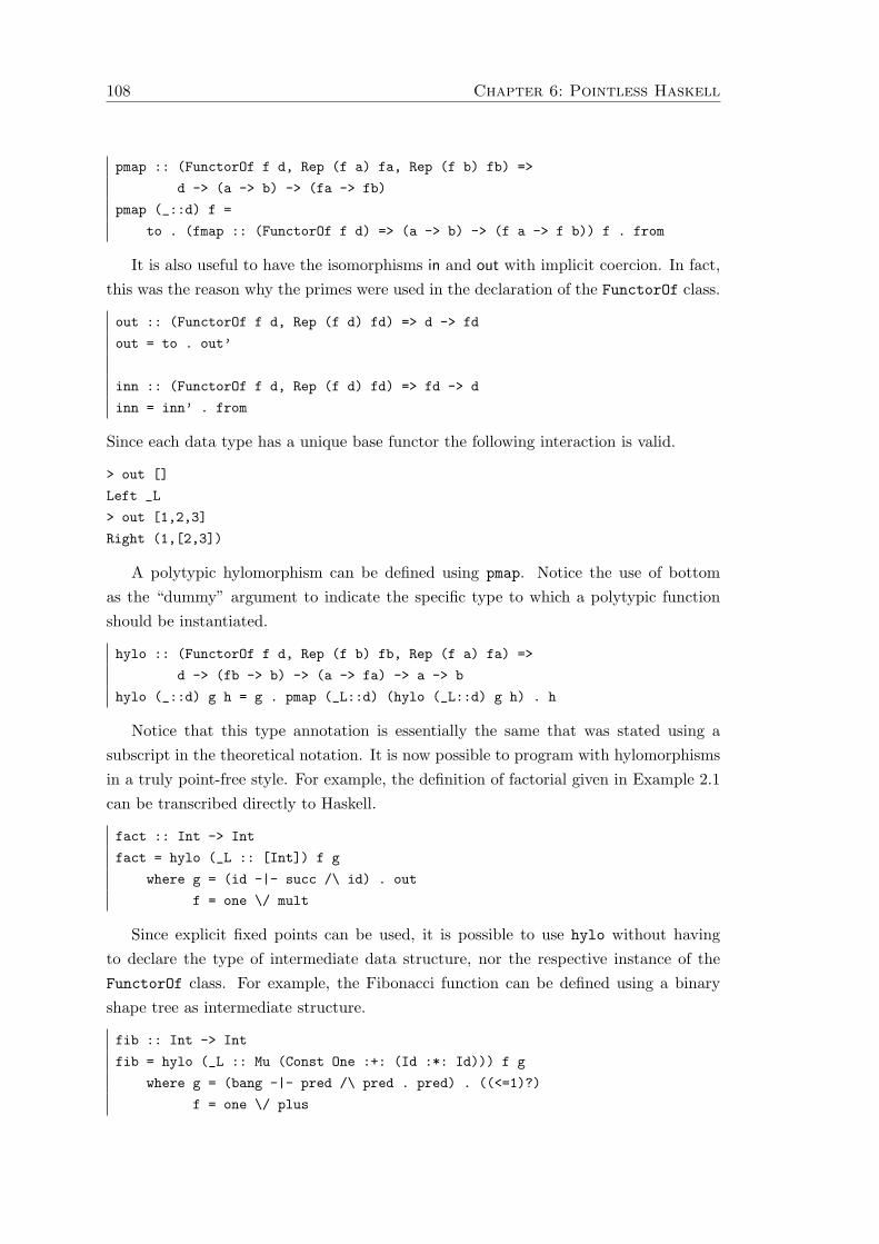
108 Chapter 6: Pointless Haskell
pmap :: (FunctorOf f d, Rep (f a) fa, Rep (f b) fb) =>
d -> (a -> b) -> (fa -> fb)
pmap (_::d) f =
to . (fmap :: (FunctorOf f d) => (a -> b) -> (f a -> f b)) f . from
It is also useful to have the isomorphisms in and out with implicit coercion. In fact,this was the reason why the primes were used in the declaration of the FunctorOf class.
out :: (FunctorOf f d, Rep (f d) fd) => d -> fd
out = to . out’
inn :: (FunctorOf f d, Rep (f d) fd) => fd -> d
inn = inn’ . from
Since each data type has a unique base functor the following interaction is valid.
> out []
Left _L
> out [1,2,3]
Right (1,[2,3])
A polytypic hylomorphism can be defined using pmap. Notice the use of bottomas the “dummy” argument to indicate the specific type to which a polytypic functionshould be instantiated.
hylo :: (FunctorOf f d, Rep (f b) fb, Rep (f a) fa) =>
d -> (fb -> b) -> (a -> fa) -> a -> b
hylo (_::d) g h = g . pmap (_L::d) (hylo (_L::d) g h) . h
Notice that this type annotation is essentially the same that was stated using asubscript in the theoretical notation. It is now possible to program with hylomorphismsin a truly point-free style. For example, the definition of factorial given in Example 2.1can be transcribed directly to Haskell.
fact :: Int -> Int
fact = hylo (_L :: [Int]) f g
where g = (id -|- succ /\ id) . out
f = one \/ mult
Since explicit fixed points can be used, it is possible to use hylo without havingto declare the type of intermediate data structure, nor the respective instance of theFunctorOf class. For example, the Fibonacci function can be defined using a binaryshape tree as intermediate structure.
fib :: Int -> Int
fib = hylo (_L :: Mu (Const One :+: (Id :*: Id))) f g
where g = (bang -|- pred /\ pred . pred) . ((<=1)?)
f = one \/ plus

6.3 A Point-free Programming Library 109
Other recursion patterns can now be defined exactly as presented in Chapter 3, withthe functor that generates the intermediate data structure explicitly stated.
cata :: (FunctorOf f d, Rep (f a) fa, Rep (f d) fd) =>
d -> (fa -> a) -> d -> a
cata (_::d) g = hylo (_L::d) g out
ana :: (FunctorOf f d, Rep (f a) fa, Rep (f d) fd) =>
d -> (a -> fa) -> a -> d
ana (_::d) h = hylo (_L::d) inn h
This approach works equally well with data types defined using type functors, suchas rose trees. Given the expected declaration of a data type Rose a, with an appropriateinstance of FunctorOf
data Rose a = Forest a [Rose a]
instance FunctorOf (Const a :*: ([] :@: Id)) (Rose a)
where inn’ (Const x :*: Comp l) = Forest x (map unId l)
out’ (Forest x l) = Const x :*: Comp (map Id l)
the preorder traversal of rose trees can be defined exactly as in Example 3.8.
preorder :: Rose a -> [a]
preorder = cata (_L::Rose a) (cons . (id >< flatten))
flatten :: [[a]] -> [a]
flatten = cata (_L::[[a]]) (nil \/ cat)
One of the advantages of this approach is that, in order to declare the more advancedrecursion patterns, we no longer need to define the functor transformers – this resultsfrom the ability to explicitly declare the intermediate data type as the fixed point of afunctor. For example, the implementations of paramorphisms and accumulations cannow be transcribed from their definitions.
para (_::d) g =
hylo (_L :: FunctorOf f d => Mu (f :@: (Id :*: Const d)))
g (pmap (_L::d) (id /\ id) . out)
accum (_::d) g t =
hylo (_L :: FunctorOf f d => Mu (f :*: (Const a)))
g ((t /\ snd) . (out >< id))
The types of these recursion operators are omitted because of their increasing complexity.Finally, we present the definitions of the factorial as a paramorphism, and of addition asan accumulation. Again, these are exactly the same as the ones presented in examples3.15 and 3.20, respectively.

110 Chapter 6: Pointless Haskell
fact :: Int -> Int
fact = para (_L::Int) g
where g = one \/ mult . (id >< succ)
plus :: (Int,Int) -> Int
plus = accum (_L::Int) g t
where t = (fst -|- id >< succ) . distl
g = (snd \/ fst) . distl
6.4 Visualization of Intermediate Data Structures
This section describes how to incorporate in Pointless Haskell a generic visualizationmechanism for the intermediate data structures of hylomorphisms. This mechanism isbased on GHood [Rei01], a graphical animation tool built on top of Hood [Gil00], theHaskell Object Observation Debugger. This feature is based on previous work on thevisualization of recursion trees of Haskell functions [Cun03]. The section starts with abrief review of Hood and GHood.
6.4.1 Hood and GHood
Hood is a portable debugger for full Haskell, based on the concept of observation ofintermediate data structures as they are passed between functions. Its author arguesthat this model is the analog, in the functional paradigm, to the traditional debuggingmethod of breakpointing and variable examination used in imperative programming.
The starting point to the implementation of Hood was the non-standard unsafefunction trace, included in all major Haskell distributions. This function has the typeString -> a -> a, and its semantics is to print the first argument as a side effectand then return the second argument. There are some problems with using trace fordebugging purposes [Gil00]:
• The biggest problem is that trace is strict in its first argument, and if we want tooutput some of the terms being evaluated the strictness properties of the observedprogram will inevitably change.
• The output tends to be incomprehensible partly due to the unintuitive orderingof lazy evaluation, and partly to the strictness on the first argument that mightsometimes trigger the evaluation of other traces.
• Its insertion on the code tends to be invasive, due to the need to convey explicitlythe outputed data in the first argument.
In order to overcome these problems, a new combinator with a similar type wasdeveloped:

6.4 Visualization of Intermediate Data Structures 111
observe :: (Observable a) => String -> a -> a
However, its semantics is considerably different from trace. The label is no longerused to output the observations, but only for identification purposes when multipleobservation points coexist in the same program. Instead of just returning the secondargument, it stores it into some persistent structure for later rendering. It behaves likean id function that somehow remembers its argument. The class restriction will beexplained later. For now it suffices to know that there are predefined instances to moststandard types.
Consider the following example presented in [Gil00]. In order to trace the executionof the following function that returns the digits of an integer
digits :: Int -> [Int]
digits = reverse .
map (‘mod‘ 10) .
takeWhile (/= 0) .
iterate (‘div‘ 10)
observe can be inserted at the places where inspection of the intermediate data struc-tures is required.
digits :: Int -> [Int]
digits = observe "after reverse" . reverse .
observe "after map" . map (‘mod‘ 10) .
observe "after takeWhile" . takeWhile (/= 0) .
observe "after iterate" . iterate (‘div‘ 10)
If this function is called with the parameter 1234, the following trace results.
-- after iterate
1234 : 123 : 12 : 1 : 0 : _
-- after map
4 : 3 : 2 : 1 : []
-- after reverse
1 : 2 : 3 : 4 : []
-- after takeWhile
1234 : 123 : 12 : 1 : []
Notice that unevaluated subexpressions are represented by underscore. The implemen-tation of the observe function manages to eliminate all the major weaknesses of trace:
• It guarantees that the strictness properties of the observed program do not change.
• The capture of information (triggered by the evaluation of observe) is decou-pled from presentation. The observations are post-processed when the programterminates, and are grouped by their labels into a structured presentation.

112 Chapter 6: Pointless Haskell
Figure 6.1: GHood screenshot
• Due to the existence of predefined instances for most standard types and a verysimple, combinator based, approach to define new instances of the class Observable,minimal changes to the program are required.
The implementation of observe is based on a helper function observer, defined asa method of the class Observable. Implementing new instances of the class Observableis rather straightforward due to the high-level combinators and monads included in thelibrary. For example, the predefined instance for lists is implemented as follows.
instance (Observable a) => Observable [a] where
observer (a:as) = send ":" (return (:) << a << as)
observer [] = send "[]" (return [])
Function send is responsible for storing the information into some persistent struc-ture for later rendering. Besides collecting information about what constructors arebeing observed, and where they are located in the data structure, the send functionalso records when the observation was done. This temporal information, that is notused by Hood’s rendering, was the departing point to the developing of GHood’s ani-mation mechanism. Instead of a text-based visualization, GHood opted for a graphicalvisualization based on a simple tree-layout algorithm. The major change to the originallibrary consisted of logging the events into a text file, so that they can be processedby an external viewer (developed in Java). For the user there are no changes at all.The final state of the animation for the same example presented above is displayed inFigure 6.1.

6.4 Visualization of Intermediate Data Structures 113
6.4.2 Instrumenting Hylomorphisms for Visualization
The key mechanism behind intermediate data structure visualization is the Hylo-Split
law, that factorizes a hylomorphism into the composition of a catamorphism with ananamorphism. The application of this law exposes the virtual data structure that rep-resents the recursion tree of the hylomorphism, and allows us to insert an observationpoint in order to record its runtime evolution. Following this approach, a new versionof the hylomorphism can be defined, to be used when visualization is desired.
hyloO (_::d) g h = cata (_L::d) g .
observe "Recursion Tree" .
ana (_L::d) h
Notice that this function behaves exactly as the former hylomorphism definition, andcan replace it in any definition, as long as the data type d belongs to the Observable
class. For example, in order to observe the recursion tree of the factorial function, itsuffices to replace hylo by hyloO in the previous definition. The list that results fromobserving fact 5 is shown in Figure 6.2, and as expected corresponds to the list of allnumbers from 5 downto 1.
fact :: Int -> Int
fact = hyloO (_L :: [Int]) f g
where g = (id -|- succ /\ id) . out
f = one \/ mult
Figure 6.2: Recursion tree of fact 5.
It is also possible to define observed versions of other recursion patterns. For exam-ple, the definition of the observed catamorphism can be
cataO (_::d) f = hyloO (_L::d) f out

114 Chapter 6: Pointless Haskell
In order to observe a hylomorphism whose intermediate data structure is given byan explicit fixed point some additional work is required. Since Mu can be applied toany arrangement of the functor combinators, a polytypic instance of the Observable
class must be defined. Such definition is the subject of the next section. Assuming itsexistence, the recursion tree of the Fibonacci function can be visualized as follows.
fib :: Int -> Int
fib = hyloO (_L :: Mu (Const One :+: Id :*: Id)) f g
where g = (bang -|- pred /\ pred . pred) . ((<=1)?)
f = one \/ plus
The binary shape tree that results from observing fib 5 is presented in Figure 6.3.Notice that the number of leaves corresponds to the output of the function.
Figure 6.3: Recursion tree of fib 5.
A couple of visualization related remarks should be made about this tree. First,unlike the factorial example, the nodes of the tree are not tagged with constructornames because in the fixpoint view they simply do not exist. Second, the thunks thatappear on the leaves correspond to unevaluated parts of the data structure. In thisparticular case, they occur because the leaves contain values of type One, that cannotbe observed without raising an exception since they are undefined. This exposes aminor drawback of the polytypic observation function, namely that it will be impossibleto distinguish an observation of the One data type from observations of unevaluatedstructures. For example, consider the following definition of the length function.
length :: Observable a => [a] -> Int
length = cataO (_L::Mu (Const One :+: Const a :*: Id)) g
where g = zero \/ succ . snd
The recursion tree of len [1,2,3] is shown in Figure 6.4. Notice that, since thisfunction is polymorphic and does not need to evaluate the elements of the list, they are

6.4 Visualization of Intermediate Data Structures 115
represented by unevaluated thunks. But the same happens with the empty list (the lastthunk in the sequence), since it is defined as the left injection of the bottom element.
Figure 6.4: Recursion tree of length [1,2,3].
The above definition of hyloO still suffers from an annoying limitation. Suppose thatone wants to observe a user-defined data type, for which an instance of the FunctorOf
class has already been defined. With the present definition of hyloO, the respectiveinstance of Observable must be defined, even if a generic observation for the isomorphicfixed point already exists. In order to redirect the visualization to that instance, andthus avoid the need to define a new one, the definition of hyloO is changed as follows.Notice the use of the explicit type parameter, and the FunctorOf class, to force thehylomorphism to build as intermediate structure an element of type Mu f instead ofthe isomorphic element of type d. This is possible because f is simultaneously the basefunctor of Mu f and d.
hyloO (_::d) g h = cata (_L::FunctorOf f d => Mu f) g .
observe "Recursion Tree" .
ana (_L::FunctorOf f d => Mu f) h
The utility of this trick is illustrated with a final example. Suppose that the instanceof FunctorOf for the Tree data type is already defined. It is well known that the quick-sort algorithm can be defined as a hylomorphism using a binary tree as an intermediatestructure [Aug99].
qsort :: (Observable a, Ord a) => [a] -> [a]
qsort = hyloO (_L::Tree a) f g
where g = (id -|- fst /\ part) . out
f = nil \/ cat . (id >< cons) . assocr . (swap >< id) . assocl
Most of the work is done by the part function, of type (a,[a]) -> ([a],[a]), thatdivides the tail into two lists: one keeps the elements that are smaller than the head of the

116 Chapter 6: Pointless Haskell
input list, and the other the remaining elements. Even without declaring the Observableinstance for Tree, the binary search tree that models the recursion tree of this definitioncan be visualized. Figure 6.5 shows the recursion tree of qsort [3,2,4,3,1].
Figure 6.5: Recursion tree of qsort [3,2,4,3,1].
6.4.3 Polytypic Observable Instances
In order to explain how a generic observer can be defined, the definition of << is expandedin the following definition of the Observable instance for lists.
instance (Observable a) => Observable [a] where
observer (a:as) = send ":" (do {a’ <- thunk a
as’ <- thunk as
return (a’:as’)})
observer [] = send "[]" (return [])
The first parameter of the send function is the tag that labels the intermediate nodesof the tree. As already mentioned, this tag will be ignored in the visualization of valuesdeclared explicitly using the fixpoint operator. The second parameter is a value in thestate ObserverM, that is executed by the send function in order to evaluate a term andsimultaneously collect information for the renderer. Function thunk is invoked for eachchild in a node, and graphically it will trigger a new branch in the tree. Even withoutpresenting more details, it is clear that the monadic code follows the structure of thetype, and so it should be possible to define generically a function for embedding a valueinto ObserverM. In order to make this idea more precise, the desired instance for thefixpoint view of the list data type is presented.
instance Observable a => Observable (Mu (Const One :+: Const a :*: Id))
where observer (Mu (Inl (Const x))) =
send "" (do x’ <- thunk x

6.4 Visualization of Intermediate Data Structures 117
return (Mu (Inl (Const x’))))
observer (Mu (Inr (Const x :*: Id y))) =
send "" (do x’ <- thunk x
y’ <- thunk y
return (Mu (Inr (Const x’ :*: Id y’))))
Notice that the thunk function is invoked for every recursive occurrence of the data typeand, in case of parameterized types, also at the content nodes (signaled by a constantin the base functor).
Following the PolyP approach, a class to contain the new polytypic function is firstdefined. For a data type µF , this function will be responsible for embedding a valueof type F (µF ) into the state monad ObserverM. It receives as parameter a monadicfunction that should be applied when the functor is the identity. The need for thisparameter will be justified later.
class FunctorO f
where fmapO :: (a -> ObserverM b) -> f a -> ObserverM (f b)
The instances for the basic set of functor combinators can be defined as follows.
instance FunctorO Id
where fmapO f (Id x) = do x’ <- f x
return (Id x’)
instance Observable a => FunctorO (Const a)
where fmapO f (Const x) = do x’ <- thunk x
return (Const x’)
instance (FunctorO f, FunctorO g) => FunctorO (f :+: g)
where fmapO f (Inl x) = do x’ <- fmapO f x
return (Inl x’)
fmapO f (Inr x) = do x’ <- fmapO f x
return (Inr x’)
instance (FunctorO f, FunctorO g) => FunctorO (f :*: g)
where fmapO f (x :*: y) = do x’ <- fmapO f x
y’ <- fmapO f y
return (x’ :*: y’)
instance (FunctorO g, FunctorO h) => FunctorO (g :@: h)
where fmapO f (Comp x) = do x’ <- fmapO (fmapO f) x
return (Comp x’)
Since thunk should only be applied at recursive values, it cannot be blindly applied ateach occurrence of the identity functor. Due to the composition combinator, the identity

118 Chapter 6: Pointless Haskell
functor may also occur in other positions. For example, the following functor can alsobe used to model lists.
Id :@: (Const One :+: Const a :*: Id)
The parameterization with a monadic function and the instance implementation for thecomposition guarantees that, if we invoke fmapO with thunk as parameter to an elementof this type, it will only be applied to the rightmost identity (the one that denotes therecursive occurrence).
The name fmapO comes from the fact that this function closely resembles a monadicmap [Fok94]. Given a monad M and a functor F , the monadic map is a function oftype (A → M B) → (F A → M (F B)) that distributes a monadic operation throughthe functor. Likewise to ordinary map, this is a well known polytypic function (over thestructure of F ), and is offered in the libraries of some generic programming languages,namely Generic Haskell [CHJ+01]. The only place where fmapO differs from a monadicmap is in the treatment of the constant functor, where it applies thunk instead of thereturn function.
Given fmapO, the implementation of the Observable instance for Mu is very simple.
instance (Functor f, FunctorO f) => Observable (Mu f)
where observer (Mu x) = send "" (do x’ <- fmapO thunk x
return (Mu x’))
Finally, the trivial instance of Observable for the terminal data type is defined.Remember that it is not possible to observe the only value of this type, unless anexception is raised. In practice that will never happen, and an unevaluated thunk willbe displayed instead.
instance Observable One
where observer _ = _L
6.5 Summary
This chapter presented a Haskell library that can be used to program with recursionpatterns in a point-free and polytypic style. The implementation of polytypic abilitiesis similar to the one in the PolyP library. To enable a truly point-free style, we definedan implicit coercion mechanism that encodes a limited form of structural equivalencebetween types. The implementation required some extensions to the standard Haskelltype system. If used without care, these extensions can make type-checking undecidable.By introducing type annotations similar to the ones used in the theoretical notation thisproblem was avoided. The main disadvantage of using this library is that, again due tothe heavy use of extensions, the error messages displayed by the compiler are of limitedhelp for the programmer.

6.5 Summary 119
We have also shown how to implement a generic mechanism for visualizing inter-mediate data structures of hylomorphisms. This feature is very useful for programunderstanding, since it graphically exposes the intermediate data structure that resultsfrom the factorization of a hylomorphism using the Hylo-Split law. Since it is based onHood, the implementation preserves the strictness properties of the original program.This feature is also very useful to identify opportunities to apply the Hylo-Shift law.For example, in the visualization of the length function, the existence of unevaluatedthunks means that, in fact, the type that parameterizes the hylomorphism can be sim-plified into a natural number, by shifting all work into the anamorphism side. Noticethat the visualized tree looks like an element of type List 1 that is isomorphic to Nat.
The Pointless Haskell library is available for download from the following web page.
http://wiki.di.uminho.pt/bin/view/Alcino/PointlessHaskell

120 Chapter 6: Pointless Haskell

Chapter 7
Deriving Point-free Definitions
This thesis advocates the use of the point-free style and recursion patterns for programcalculation and transformation. However, it is a fact that most programmers use explicitrecursion instead of recursion patterns, and probably no one uses a pure point-free style.In this chapter we show how pointwise definitions can be converted into the point-freestyle, and how to replace explicit recursion by hylomorphisms. The idea is to enableone to program in one style, and automatically move to the other in order to performproofs and calculations. A useful comparison here is that of mathematical transformssuch as the Fourier transform or the Laplace transform, which allow to express functionsin different domains in which certain manipulations are easier to perform.
The well-known equivalence between simply-typed λ-calculus (with pairs and ter-minal object) and cartesian closed categories was first suggested by Lambek [Lam80].This equivalence includes a translation from pointwise terms to categorical combinators,that was later used by Curien to define a new implementation technique for functionallanguages – the categorical abstract machine [Cur93]. This translation is also the start-ing point to our point-free derivation mechanism. We show how it can be extendedto handle sums and recursion. For recursion two different techniques will be used: adirect encoding of the fixpoint operator using hylomorphisms; and the hylomorphismderivation algorithm of Hu, Iwasaki, and Takeichi [HIT96]. We also show how this coreλ-calculus can be used to encode structured types and pattern matching. In practice,this means that the translation can be applied to a reasonable subset of most modernfunctional programming languages, namely Haskell. A standard denotational semanticsof λ-calculus based on pcpos is assumed.
7.1 Typed λ-Calculi and Cartesian Closed Categories
This section briefly presents a typed λ-calculus with products and a terminal object,and its translation to cartesian closed categories. Given a set of base types Σ, types are
121

122 Chapter 7: Deriving Point-free Definitions
determined by the following grammar, where α ∈ Σ.
A ::= α (Base types)| 1 (Terminal type)| A×A (Pairs)| A → A (Functions)
The set of raw typed λ-terms is given by the following grammar, were c denotes aconstant with type ∆(c), and x ranges over variables.
M ::= ? (Unit)| c (Constant)| x (Variable)| λx : A.M (Abstraction)| (MM) (Application)| 〈M,M〉 (Pairing)| fst(M) (First projection)| snd(M) (Second projection)
The usual notions of free and bound variable are defined on terms. FV(M) denotesthe set of free variables in M , and M [N/x] the capture-avoiding substitution of N forthe free occurrences of x in M . Typing rules are expressed in terms of typing judgmentsΓ ` M : A, where M is a term, A a type, and Γ is a typing context – a list of typedeclarations for the free variables in M . All variables in a context are assumed to bedifferent, and can be reordered implicitly. The valid type judgments of this λ-calculusare those that can be derived from the following set of typing rules. A term in a validtype judgment is said to be well typed.
Γ ` ? : 1 Γ ` c : ∆(c) Γ, x : A ` x : A
Γ, x : A ` M : B
Γ ` λx : A.M : A → B
Γ ` M : A → B Γ ` N : A
Γ ` MN : B
Γ ` M : A Γ ` N : B
Γ ` 〈M,N〉 : A×B
Γ ` M : A×B
Γ ` fst(M) : A
Γ ` M : A×B
Γ ` snd(M) : B
The equational theory of this typed λ-calculus is the least typed congruence gen-erated by the following equations (modulo α-equivalence). It will be denoted by =λ.Typing information is given in the η-equations since they can only be applied to terms

7.1 Typed λ-Calculi and Cartesian Closed Categories 123
of a specific type.
M =λ ? ⇐ M : 1 Eta-Unit
(λx : A.M)N =λ M [N/x] Beta-Func
M =λ λx : A.Mx ⇐ M : A → B ∧ x 6∈ FV(M) Eta-Func
fst(〈M,N〉) =λ M ∧ snd(〈M,N〉) = N Beta-Pair
M =λ 〈fst(M), snd(M)〉 ⇐ M : A×B Eta-Pair
Example 7.1 (Swap). To exemplify the use of =λ, the isomorphism between A × B
and B ×A is proved. The same proof was given in the point-free style in Chapter 2.
swap : A×B → B ×A
swap = λx.〈snd(x), fst(x)〉
26666666666666666666664
swap (swap M)
=λ {Definition of swap }(λx.〈snd(x), fst(x)〉) ((λx.〈snd(x), fst(x)〉) M)
=λ {Beta-Func }(λx.〈snd(x), fst(x)〉) 〈snd(M), fst(M)〉
=λ {Beta-Func }〈snd(〈snd(M), fst(M)〉), fst(〈snd(M), fst(M)〉)〉
=λ {Beta-Pair }〈fst(M), snd(M)〉
=λ {Eta-Pair }M
Translation
The translation from the typed λ-calculus (pointwise) to the internal language of a carte-sian closed category (point-free) is rather ingenious. It is detailed in many text bookson the subject [LS86, Pie91, AL91, Cro93]. The way variables are handled resembles thetranslation of the lambda calculus into the de Bruijn notation [dB72], where variablesare represented by integers that “measure” the distance to the abstraction were theywhere bound. In the present case, the typing context that contains the bound variablesis represented by a left-nested pair, and a variable will be replaced by the path to itsposition in that tuple.
We begin with the interpretation of types. The function that translated types andtyping contexts to objects will be denoted by O( · ). It is assumed that each base typeA in Σ is represented by an object in the category, denoted by O(A). For the remaining

124 Chapter 7: Deriving Point-free Definitions
types the translation is defined as expected.
O(1) = 1
O(A×B) = O(A)×O(B)O(A → B) = O(B)O(A)
Assuming that ε denotes the empty context, the object that represents a typingcontext is generated as follows.
O(ε) = 1
O(Γ, x : A) = O(Γ)×O(A)
The translation from λ-terms to morphisms in the category will be denoted by thefunction M( · ). To be more precise, this function operates on typing judgments. Ajudgment Γ ` M : A will be interpreted as a morphism
M(Γ ` M : A) : O(Γ) → O(A)
according to the following rules. In order to simplify the presentation, type annotationsare omitted from the basic categorical combinators.
M(Γ ` ? : 1) = !M(Γ ` c : A) = c ◦ !M(Γ, x : A ` x : A) = snd
M(Γ, y : A ` x : B) = M(Γ ` x : B) ◦ fst ⇐ x 6= y
M(Γ ` λx : A.M : A → B) = M(Γ, x : A ` M : B)M(Γ ` MN : A) = ap ◦ (M(Γ ` M : B → A) MM(Γ ` N : B))M(Γ ` 〈M,N〉 : A×B) = M(Γ ` M : A) MM(Γ ` N : B)M(Γ ` fst(M) : A) = fst ◦M(Γ ` M : A×B)M(Γ ` snd(M) : B) = snd ◦M(Γ ` M : A×B)
Notice that in the rules for application and projections, the type of M can be obtainedby type inference using the rules presented before.
The translation of a closed term M : A → B is the point that represents it in thecategory, that is, a morphism of type 1 → O(B)O(A). As seen in Chapter 2, since thecategory is cartesian closed, this point can be converted into the expected morphismof type A → B using Pnt-Cancel. As such, for closed terms of functional type thetranslation is defined as follows.
ap ◦ (M(` M : A → B) ◦ ! M id)
Example 7.2 (Identity). For example, the identity function λx : A.x is translated

7.1 Typed λ-Calculi and Cartesian Closed Categories 125
intosnd : 1 → AA
Since this is a closed term of functional type, it is possible to convert the result to amorphism of type A → A and prove that it is indeed equivalent to id.
2666666666664
ap ◦ (snd ◦ ! M id)
= {Prod-Absor }ap ◦ (snd× id) ◦ (! M id)
= {Exp-Cancel }snd ◦ (! M id)
= {Prod-Cancel }id
Example 7.3 (Swap). For the swap function defined in Example 7.1 we get the fol-lowing translation.
snd ◦ snd M fst ◦ snd : 1 → B ×AA×B
Again, since it is of functional type, some simple calculations show that it is equivalentto the expected definition.
266666666666666664
ap ◦ (snd ◦ snd M fst ◦ snd ◦ ! M id)
= {Prod-Absor }ap ◦ (snd ◦ snd M fst ◦ snd× id) ◦ (! M id)
= {Exp-Cancel }(snd ◦ snd M fst ◦ snd) ◦ (! M id)
= {Prod-Fusion }snd ◦ snd ◦ (! M id) M fst ◦ snd ◦ (! M id)
= {Prod-Cancel }snd M fst
Soundness
It can be shown that this translation is sound, i.e, that all equivalences proved using=λ can also be proved in the categorical setting using the equational theory presentedin Chapter 2. Because of its length we omit the full proof of this fact. The interestedreader can check it, for example, in [Cur93, Mar96]. Since the equational laws relatedto products have a direct correspondence in the categorical side, the most interestingpart of the proof concerns Beta-Func and Eta-Func. The fundamental result is that theconcept of substitution is replaced by that of composition. Consider the following typingrule for substitution.
Γ, x : A ` M : B Γ ` N : A
Γ ` M [N/x] : B

126 Chapter 7: Deriving Point-free Definitions
Assuming that the object that results from the translation of a context or a type isdenoted by the same identifier, we have that
M(Γ, x : A ` M : B) : Γ×A → B
M(Γ ` N : A) : Γ → A
M(Γ ` M [N/x] : B) : Γ → B
Then, it can be proved by structural induction on M that
M(Γ ` M [N/x] : B) = M(Γ, x : A ` M : B) ◦ (id MM(Γ ` N : A))
The soundness of the translation concerning Beta-Func follows trivially from thislemma.
266666666666666664
M(Γ ` (λx : A.M)N : B)
= {Translation of application }ap ◦ (M(Γ ` (λx : A.M) : A → B) MM(Γ ` N : A))
= {Translation of abstraction }ap ◦ (M(Γ, x : A ` M : B) MM(Γ ` N : A))
= {Prod-Absor, Exp-Cancel }M(Γ, x : A ` M : B) ◦ (id MM(Γ ` N : A))
= {Above lemma }M(Γ ` M [N/x] : B)
7.2 Sums
We will now enrich this λ-calculus with sums.
A ::= . . .
| A + A (Sums)
At the term level, it is augmented with case analysis and injections.
M ::= . . .
| case(M,M,M) (Case analysis)| inlA(M) (First injection)| inrA(M) (Second injection)
The typing rules for these constructs are as follows.
Γ ` L : A + B Γ ` M : A → C Γ ` N : B → C
Γ ` case(L,M,N) : C
Γ ` M : A
Γ ` inlA(M) : A + B
Γ ` M : B
Γ ` inrB(M) : A + B

7.2 Sums 127
Typically, the case expression will be used together with lambda abstractions, in theform case(L, λx : A.M, λy : B.N). In Haskell, and assuming that sum is implementedby the Either data type, this expression corresponds to
case L of (Left x ) -> M ; (Right y ) -> N
Concerning the equational theory, the following equivalences hold.
case(inl(L),M, N) =λ ML ∧ case(inr(L),M, N) =λ NL Beta-Case
MN =λ case(N,λx : A.M(inl(x)), λy : B.M(inr(y)))⇐
x, y 6∈ FV(M) ∧ N : A + B ∧ M strict
Eta-Case
Given the pcpo semantics, a case expression diverges when its first argument diverges.This fact justifies the strictness side condition in Eta-Case.
Translation
Our approach to the translation of sums is slightly different from other published works,such as [Cro93]. The injections are handled straightforwardly.
M(Γ ` inl(M) : A + B) = inl ◦M(Γ ` M : A)M(Γ ` inr(M) : A + B) = inr ◦M(Γ ` M : B)
The case translation is more difficult. We will first give an intuition of how it works.Notice that case(L,M,N) : C is equivalent to (M ON)L (defined in a mixed, pointwiseand point-free, style). This equivalence exposes the fact that a case is just an instanceof application, and as such its translation exhibits the same top level structure:
O(Γ)M(Γ`MON)MM(Γ`L)// O(CA+B × (A + B))
ap // O(C)
The question remains of how to combine M(Γ ` M : A → C) and M(Γ ` N : B →C) in order to obtain the equivalent of M(Γ ` M ON : A + B → C). Our solution isbased on the internalization of the either combinator, that can be defined as follows.
either : CA × CB → CA+B
either = (ap O ap) ◦ (fst× id + snd× id) ◦ distrEither-Def
To show that this definition is correct we show that its action on a pair of points yieldsthe expected result. This calculation uses some properties about distr that are statedand proved in Appendix A.
either ◦ (f M g) = f O g Either-Pnt

128 Chapter 7: Deriving Point-free Definitions
266666666666666666666666666666664
either ◦ (f M g)
= {Either-Def }(ap O ap) ◦ (fst× id + snd× id) ◦ distr ◦ (f M g)
= {Exp-Fusion, Sum-Functor-Id }(ap O ap) ◦ (fst× id + snd× id) ◦ distr ◦ ((f M g)× (id + id))
= {Distr-Nat }(ap O ap) ◦ (fst× id + snd× id) ◦ ((f M g)× id + (f M g)× id) ◦ distr
= {Sum-Functor-Comp, Prod-Functor-Comp, Prod-Cancel }(ap O ap) ◦ (f × id + g × id) ◦ distr
= {Pnt-Def, Sum-Absor, Exp-Cancel }(f ◦ snd O g ◦ snd) ◦ distr
= {Sum-Absor, Distr-Snd }(f O g) ◦ snd
= {Pnt-Def }f O g
Notice that, given f : A → B, in the definition f = f ◦ snd the projection snd hastype 1 × A → A. However, the above proof is independent of this fact, and thus thefollowing more general law is also valid.
either ◦ (f ◦ snd M g ◦ snd) = (f O g) ◦ snd Either-Const
Given this combinator, the translation of the case is defined as
M(Γ ` case(L,M,N) : C)=
ap ◦ (either ◦ (M(Γ ` M : A → C) MM(Γ ` N : B → C)) MM(Γ ` L : A + B))
Example 7.4 (Coswap). In order to exemplify the translation of sums, consider itsapplication to the pointwise definition of coswap.
coswap : A + B → B + A
coswap = λx.case(x, λy.inr(y), λz.inl(z))
The following result is obtained.
ap ◦ (either ◦ (inr ◦ snd M inl ◦ snd) M snd) : 1 → B + AA+B
The following calculation shows that this expression corresponds to the definition Coswap-
Def.

7.2 Sums 129
266666666666666664
ap ◦ (ap ◦ (either ◦ (inr ◦ snd M inl ◦ snd) M snd) ◦ ! M id)
= {Prod-Absor, Exp-Cancel }ap ◦ (either ◦ (inr ◦ snd M inl ◦ snd) M snd) ◦ (! M id)
= {Either-Const }ap ◦ ((inr O inl) ◦ snd M snd) ◦ (! M id)
= {Prod-Absor, Exp-Cancel }(inr O inl) ◦ snd ◦ (id M snd) ◦ (! M id)
= {Prod-Cancel }inr O inl
Soundness
To prove that this translation is sound concerning Beta-Case and Eta-Case, the followingfacts should be proved using the equational theory of categorical combinators.
M(Γ ` case(inl(L),M, N)) = M(Γ ` ML)M(Γ ` case(inr(L),M,N)) = M(Γ ` NL)
M(Γ ` MN) = M(Γ ` case(N,λx : A.M(inl(x)), λy : B.M(inr(y))))⇐
x, y 6∈ FV(M) ∧ N : A + B ∧ M strict
To simplify the proof it is convenient to restate the laws for sums using the in-ternalized version of the either combinator. Sum-Cancel can be defined and proved asfollows.
•inl ◦ either = fst ∧ •inr ◦ either = snd Either-Cancel
2666666666666666666666666664
•inl ◦ either
= {Pxe-Def }ap ◦ (id× inl) ◦ either
= {Exp-Fusion, Prod-Functor-Comp }ap ◦ (either × inl)
= {Prod-Functor-Comp, Either-Def, Exp-Cancel }(ap O ap) ◦ (fst× id + snd× id) ◦ distr ◦ (id× inl)
= {Distr-Cancel }(ap O ap) ◦ (fst× id + snd× id) ◦ inl
= {Sum-Absor, Sum-Cancel }ap ◦ (fst× id)
= {Exp-Fusion, Exp-Reflex }fst
As usual, we omit the similar proof for right injection. Notice that, due to Exp-Equal,Either-Cancel can alternatively be defined in uncurried form as follows.
ap ◦ (either × inl) = ap ◦ (fst× id)ap ◦ (either × inr) = ap ◦ (snd× id)
Either-Cancel-Alt

130 Chapter 7: Deriving Point-free Definitions
For the remaining laws, namely Sum-Reflex and Sum-Fusion, a formulation usingeither is more difficult due to the strictness side conditions. First, notice that both theselaws can be replaced by the following, that resembles Eta-Case at the point-free level.The proof of this equivalence is quite easy and is omitted.
f ◦ inl O f ◦ inr = f ⇐ f strict Eta-Sum
Strict application. Consider a strict application operator sap : BA×A → B definedby the following equations.
sap (f, x) =
{⊥ if x = ⊥f x otherwise
Then sap : BA → BA is a strictify operator, that transforms any function into its strictversion. The experienced Haskell programmer certainly recognizes this function, since itis predefined in the language as follows, and is widely used to avoid unneeded laziness.
($!) :: (a -> b) -> (a -> b)
f $! x = x ‘seq‘ f x
This implementation uses the standard seq function, that verifies the following equa-tions. Notice that this function cannot be defined within the language, but must beprovided by all compilers and interpreters.
seq x y =
{⊥ if x = ⊥y otherwise
Given strict f it is obvious that sap f = f . In general, given a function f : A → BC
that returns a strict function, sap ◦ f = f holds. A function of this type returns a strictfunction if its uncurried version is right-strict. This concept is formalized as follows.
f right-strict ⇔ f ◦ (id×⊥) = ⊥ ◦ snd Rstrict-Def
sap ◦ f = f ⇐ ap ◦ (f × id) right-strict Sap-Cancel
Likewise to seq, it is not possible to define sap in general using the basic set ofcategorical combinators. However, for the particular case of arguments of sum type itcan be defined. In Section 2.2 we have seen that distr ◦ undistr = id, but the same is nottrue for undistr ◦ distr : A× (B + C) → A× (B + C). Given a value (x,⊥), distr returns⊥ and thus undistr cannot recover the initial value, and also returns ⊥. This fact, thatmakes CPO a non-distributive category, can be used to define the following instance ofsap for sums.
sap : C(A+B) × (A + B) → C
sap = ap ◦ undistr ◦ distrSap-Def

7.2 Sums 131
If the second component of the input pair is not ⊥, the function in the first componentis applied to it. Otherwise, undistr ◦ distr returns ⊥C(A+B)×(A+B) = (⊥C(A+B) ,⊥A+B),and since ⊥C(A+B) is the function that always returns bottom, the application yields⊥C , as desired.
With the strictify operator, Eta-Sum can be restated, without an explicit strictnessside-condition, as f ◦ inl O f ◦ inr = sap f . This law can now be internalized using theeither combinator.
either ◦ (•inl M •inr) = sap Eta-Either
2666666666666666666666666666666666666666664
either ◦ (•inl M •inr)
= {Either-Def }(ap O ap) ◦ (fst× id + snd× id) ◦ distr ◦ (•inl M •inr)
= {Exp-Fusion, Sum-Functor-Id }(ap O ap) ◦ (fst× id + snd× id) ◦ distr ◦ ((•inl M •inr)× (id + id))
= {Distr-Nat }(ap O ap) ◦ (fst× id + snd× id) ◦ (((•inl M •inr)× id) + ((•inl M •inr)× id)) ◦ distr
= {Prod-Functor-Comp, Prod-Cancel }(ap O ap) ◦ (•inl× id + •inr × id) ◦ distr
= {Pxe-Def, Sum-Absor }(ap ◦ (ap ◦ (id× inl)× id) O ap ◦ (ap ◦ (id× inr)× id)) ◦ distr
= {Exp-Cancel }(ap ◦ (id× inl) O ap ◦ (id× inr)) ◦ distr
= {Sum-Fusion, Ap-Lstrict, Lstrict-Strict }ap ◦ ((id× inl) O (id× inr)) ◦ distr
= {Undistr-Def }ap ◦ undistr ◦ distr
= {Sap-Def }sap
Given this basic set of laws the soundness proof is much easier. As expected, theproof concerning the Beta-Case equations uses the cancellation law of either.
2666666666666666666666666664
M(Γ ` case(inl(L), M, N))
= {Translation of case }ap ◦ (either ◦ (M(Γ ` M) MM(Γ ` N)) MM(Γ ` inl(L)))
= {Translation of injection }ap ◦ (either ◦ (M(Γ ` M) MM(Γ ` N)) M inl ◦M(Γ ` L))
= {Prod-Absor }ap ◦ (either × inl) ◦ ((M(Γ ` M) MM(Γ ` N)) MM(Γ ` L))
= {Either-Cancel-Alt }ap ◦ (fst× id) ◦ ((M(Γ ` M) MM(Γ ` N)) MM(Γ ` L))
= {Prod-Absor, Prod-Cancel }ap ◦ (M(Γ ` M) MM(Γ ` L))
= {Translation of application }M(Γ ` ML)

132 Chapter 7: Deriving Point-free Definitions
The soundness proof concerning Eta-Case uses the following lemma, stating that avariable that is not used in a term can be removed from the context.
M(Γ, x : A ` M) = M(Γ ` M) ◦ fst ⇐ x 6∈ FV(M) Drop-Var
This can be proved by structural induction on the shape of M , as shown in [Mar96] forthe cartesian closed subset. The extension of this proof to cover sums is trivial.
Another fact about the translation is that a strict function of type A → B is con-verted into a function Γ → BA that returns a strict function. As such, due to Sap-Cancel
the following lemma holds.
sap ◦M(Γ ` M) = M(Γ ` M) ⇐ M strict Strict-Trans
We first prove that
M(γ ` λx : A.M(inl(x))) = •inl ◦M(Γ ` M)M(γ ` λx : A.M(inr(x))) = •inr ◦M(Γ ` M)
⇐ x 6∈ FV(M) Aux
26666666666666666666666666666666666664
M(Γ ` λx : A.M(inl(x)))
= {Translation of abstraction }M(Γ, x : A ` M(inl(x)))
= {Translation of application }ap ◦ (M(Γ, x : A ` M) MM(Γ, x : A ` inl(x)))
= {Drop-Var, x 6∈ FV(M) }ap ◦ (M(Γ ` M) ◦ fst MM(Γ, x : A ` inl(x)))
= { Injection translation }ap ◦ (M(Γ ` M) ◦ fst M inl ◦M(Γ, x : A ` x))
= {Variable translation }ap ◦ (M(Γ ` M) ◦ fst M inl ◦ snd)
= {Prod-Def }ap ◦ (M(Γ ` M)× inl)
= {Prod-Functor-Comp, Exp-Fusion }ap ◦ (id× inl) ◦M(Γ ` M)
= {Pxe-Def }•inl ◦M(Γ ` M)
Soundness concerning Eta-Case can then be proved by the following calculation.

7.3 Explicit Recursion 133
2666666666666666666666666664
M(Γ ` case(N, λx : A.M(inl(x)), λy : B.M(inr(y))))
= {Translation of case }ap ◦ (either ◦ (M(Γ ` λx : A.M(inl(x))) MM(Γ ` λy : B.M(inr(y)))) MM(Γ ` N))
= {Aux, x 6∈ FV(M), y 6∈ FV(M) }ap ◦ (either ◦ (•inl ◦M(Γ ` M) M •inr ◦M(Γ ` M)) MM(Γ ` N))
= {Prod-Fusion }ap ◦ (either ◦ (•inl M •inr) ◦M(Γ ` M) MM(Γ ` N))
= {Eta-Either }ap ◦ (sap ◦M(Γ ` M) MM(Γ ` N))
= {Strict-Trans }ap ◦ (M(Γ ` M) MM(Γ ` N))
= {Translation of application }M(Γ ` MN)
7.3 Explicit Recursion
Instead of working with a fixed set of base types and a set of constants to manipulatethem, we will incorporate in our λ-calculus the theory of recursive data types presentedin Section 2.3. To be more specific, at the type level we have
A ::= . . .
| µ(F ) (Recursive data type)
where F is a regular functor, whose operation on types is defined as expected. Atthe term level the generic constructor and destructor, and the fixpoint operator areintroduced.
M ::= . . .
| in(M) (Constructor)| out(M) (Destructor)| fix(M) (Fixpoint)
The typing rules are
Γ ` M : F (µ(F ))Γ ` in(M) : µ(F )
Γ ` M : µ(F )Γ ` out(M) : F (µ(F ))
Γ ` M : A → A
Γ ` fix(M) : A
The characterization of the fixpoint operator includes the following equation (for acomplete theory see [SP00]).
fix(M) =λ M(fix(M)) Beta-Fix

134 Chapter 7: Deriving Point-free Definitions
Translation
The translation of the constructors and destructors is trivial.
M(Γ ` in(M) : µ(F )) = in ◦M(Γ ` M : F (µ(F )))M(Γ ` out(M) : F (µ(F ))) = out ◦M(Γ ` M : µ(F ))
For the fixpoint operator the translation uses the definition of fix using a hylomor-phism, presented in section 2.4. The intermediate data structure of the hylomorphismis a stream of functions of type A → A.
M(Γ ` fix(M) : A) = [[ap, id M id]] ◦M(Γ ` M : A → A)
Example 7.5 (Repeat). We now give a simple example of translating a recursivefunction defined over a recursive data type. Consider the function that given an elementgenerates an infinite stream with copies of that value. It is quite similar to the onedefined in Example 3.12 for lists. As seen in Section 2.4, streams of elements of type A
are defined as the fixed point of A × Id. In the point-free style this function could bedefined as follows.
repeat : A → Stream A
repeat = bd(id M id)ceStream A
Using the λ-calculus presented this chapter, a possible definition is
repeat : A → Stream A
repeat = λx.fix(λy.in(〈x, y〉))
By applying the translation rules to this definition we get the following point-free ex-pression. In this case, the intermediate data structure of the hylomorphism that encodesfix is a stream of functions of type Stream A → Stream A.
fix ◦ in ◦ (snd ◦ fst M snd) : 1 → (Stream A)A
The following calculation shows that this expression is indeed equivalent to the aboveanamorphism.

7.3 Explicit Recursion 135
26666666666666666666666666666666664
ap ◦ (fix ◦ in ◦ (snd ◦ fst M snd) ◦ ! M id)
= {Prod-Absor, Exp-Cancel }fix ◦ in ◦ (snd ◦ fst M snd) ◦ (! M id)
= {Prod-Absor, Prod-Reflex }fix ◦ in ◦ (snd× id) ◦ (! M id)
= {Exp-Fusion, Prod-Cancel }fix ◦ in
= {Fix-Def, Hylo-Fusion }264 (id M id) ◦ in = (id× in) ◦ (in M id)
= {Prod-Fusion, Prod-Absor }in M in = in M in
[[ap, in M id]]
= {Prod-Absor, in× id : A× Id.→ (Stream A → Stream A)× Id }
[[ap ◦ (in× id), id M id]]
= {Exp-Cancel, Ana-Def }bd(id M id)ce
Example 7.6 (Repeat). Notice that the repeat function can also be defined as follows.
repeat : A → Stream A
repeat = fix(λy.λx.in(〈x, y x〉))
In this case, the translation rules yield the following point-free expression.
fix ◦ in ◦ (snd M ap ◦ (snd ◦ fst M snd))
To prove that this is also equal to the expected anamorphism, some simplifications arefirst performed.
266666666666666666666666666666666666664
ap ◦ (fix ◦ in ◦ (snd M ap ◦ (snd ◦ fst M snd)) ◦ ! M id)
= {Prod-Def }ap ◦ (fix ◦ in ◦ (snd M ap ◦ (snd× id)) ◦ ! M id)
= {Prod-Def, Prod-Cancel }ap ◦ (fix ◦ in ◦ (snd ◦ (snd× id) M ap ◦ (snd× id)) ◦ ! M id)
= {Prod-Fusion, Exp-Fusion }ap ◦ (fix ◦ in ◦ (snd M ap) ◦ snd ◦ ! M id)
= {Exp-Fusion,Prod-Def, Prod-Cancel }ap ◦ (fix ◦ in ◦ (snd M ap) ◦ snd M id)
= {Fix-Def, Hylo-Fusion }ap ◦ ([[ap, in ◦ (snd M ap) ◦ snd M id]] M id)
= {Prod-Absor, Hylo-Shift, † }ap ◦ ([[ap ◦ (in ◦ (snd M ap) ◦ snd× id), id M id]] M id)
= {Exp-Cancel }ap ◦ ([[in ◦ (snd M ap) ◦ snd, id M id]] M id)
= {Hylo-Shift, snd : A× Id.→ Id, Prod-Cancel }
ap ◦ ([[in ◦ (snd M ap), id]] M id)

136 Chapter 7: Deriving Point-free Definitions
Concerning †, notice that
in ◦ (snd M ap) ◦ snd× id : ((Stream A)A .→ (Stream A)A)× Id → A× Id
and notice also that, in the final hylomorphism, the intermediate data structure is µ(Id).Ana-Uniq can be used to prove that this strange expression is indeed equivalent to theexpected anamorphism.266666666666666664
out ◦ ap ◦ ([[in ◦ (snd M ap), id]] M id)
= {Hylo-Cancel }out ◦ ap ◦ (in ◦ (snd M ap) ◦ [[in ◦ (snd M ap), id]] M id)
= {Prod-Absor, Exp-Cancel }out ◦ in ◦ (snd M ap) ◦ ([[in ◦ (snd M ap), id]] M id)
= { In-Out-Iso, Prod-Fusion, Prod-Cancel }id M ap ◦ ([[in ◦ (snd M ap), id]] M id)
= {Prod-Absor }(id× ap ◦ ([[in ◦ (snd M ap), id]] M id)) ◦ (id M id)
7.4 Deriving Hylomorphisms from Recursive Definitions
This last example shows that calculating with the derived point-free expressions cansometimes be quite difficult. This is largely due to the fact that hylomorphisms areintroduced only to encode the fixpoint operator, yielding definitions very different fromthose one would get if making the derivation by hand. Ideally, one would like theresulting hylomorphisms to be more informative about the original function definition,in the sense that the intermediate data structure should model its recursion tree.
Hu, Iwasaki, and Takeichi have defined an algorithm that derives such hylomor-phisms from an explicitly recursive definition [HIT96]. This algorithm was developed tobe used in the fusion system HYLO [OHIT97], that uses the acid rain laws presented inSection 2.4 to perform deforestation. Basically, the algorithm mechanizes the informalprocess that has been used to derive hylomorphisms in Section 2.4. It has several limi-tations, namely it can not handle mutual or nested recursion, but it covers most of theuseful function definitions.
In the present context, the idea is to use this algorithm in a stage prior to thepoint-free translation defined in the previous sections. First, a pointwise hylomorphismis derived, and then the translation is applied to the algebra and the coalgebra thatparameterize it. The main difference between the presentation given in [HIT96] and theone given here lies in the underlying λ-calculus. While the original formulation allowedfor user defined types a la Haskell and general pattern matching, in our λ-calculusdata types are declared as fixed points, and pattern matching is restricted to sums. In[OHIT97] some extensions were made in order to cover more language constructs, butsince we found some errors in those extensions the presentation will be restricted to thebasic algorithm presented in [HIT96].

7.4 Deriving Hylomorphisms from Recursive Definitions 137
The hylomorphism derivation can be summarized as follows. Given a single-parameterrecursive function defined using fixpoint
fix(λf.λx.L) : A → B
we will define three transformations: one to derive the functor that generates the inter-mediate data type (F), a second one to derive the algebra (A), and another one for thecoalgebra (C). The above function will be translated into the following hylomorphism,where a dot on top of an identifier signals the creation of a fresh variable.
[[λz.A(L, z), λx.C(L)]]µ(F(L)) : A → B
Some restrictions are imposed on the syntax used to define recursive functions. Thefirst is that the definition must be a closed expression, that is FV(L) = {f, x}. Thisrestriction guarantees that the algebra and the coalgebra are also closed. If that was notthe case, it would be necessary to propagate the typing context inside the hylomorphism.This can only be achieved by changing the intermediate data structure, in a similar wayto the accumulation recursion pattern presented in Section 3.5. Of course, the algebraand the coalgebra would also need to be modified, and the translation would producehylomorphisms as unmanageable as the ones obtained by direct encoding of the fixpointoperator.
The second restriction is that the body L of the function fix(λf.λx.L) to be translatedmust be defined in two stages, according to the following grammar.
L ::= case(M,λx.L, λx.L) ⇐ f 6∈ FV(M)| N
N ::= ?
| c
| x ⇐ x 6= f
| (f N) ⇐ f 6∈ FV(N)| (N N)| 〈N,N〉| g(N) ⇐ g ∈ {fst, snd, inl, inr, in, out}
Notice that M denotes the grammar of the full λ-calculus defined in the previous sec-tions, and that x ranges over variables. Throughout this section, we also assume that f
is the distinguished identifier of the variable in the first abstraction of the fixpoint.A function is thus defined by a decision tree, implemented by case analysis on the
input, whose leaves are the different possible outputs. Although it may seem veryrestrictive, this grammar covers a lot of interesting functions, as we will shortly see.One of the main limitations in expressiveness is the absence of abstractions, which

138 Chapter 7: Deriving Point-free Definitions
prevents the definition of some higher-order functions, like the accumulations defined inChapter 4.
The three transformations are now presented in turn. To be precise, they should bedefined over typing judgments, but to simplify the presentation the contexts and typeswill be omitted. The transformation that generates the functor is defined as follows.
F(case(L, λx.M, λy.N)) = F(M) + F(N)F(?) = 1
F(c) = 1
F(x : A) = A
F(f M) = Id
F(M N) = F(M) × F(N)F(〈M,N〉) = F(M) × F(N)F(g(M)) = F(M) ⇐ g ∈ {fst, snd, inl, inr, in, out}
This transformation yields a summand for each path along the decision tree. Eachsummand signals the presence of a recursive invocation using the identity functor. Italso has place-holders for the input-dependent information that should be propagatedunchanged from the coalgebra to the algebra. Since abstractions are not allowed, aconstant functor of appropriate type is introduced for every variable outside a recursiveinvocation.
The definition of the coalgebra is very simple. It uses the same case analysis patternof the original function in order to put all the relevant information in the correct places.
C(case(L, λx.M, λy.N)) = case(L, λx.inl(C(M)), λy.inr(C(N)))C(?) = ?
C(c) = ?
C(x) = x
C(f M) = M
C(M N) = 〈C(M), C(N)〉C(〈M,N〉) = 〈C(M), C(N)〉C(g(M)) = C(M) ⇐ g ∈ {fst, snd, inl, inr, in, out}
The generation of the algebra is a little more complicated, because each variableand recursive call must be replaced by the path to the place where it was stored by the

7.4 Deriving Hylomorphisms from Recursive Definitions 139
coalgebra. In order to achieve this, an accumulator with the current path is used.
A(case(L, λx.M, λy.N), E) = case(E, λx.A(M,x), λy.A(N, y))A(?,E) = ?
A(c, E) = c
A(x,E) = E
A(f M, E) = E
A(M N, E) = (A(M, fst(E)) A(N, snd(E)))A(〈M,N〉, E) = 〈A(M, fst(E)),A(N, snd(E))〉A(g(M), E) = g(A(M), E) ⇐ g ∈ {fst, snd, inl, inr, in, out}
Without further optimizations, these transformations generate some redundancy inthe intermediate data structure of the hylomorphism. In fact, it is not necessary to storeelements of type 1 for all constants. A useful simplification that can be implementedover pairing and application, is to create a tuple only if variables or recursive calls appearon both sub-terms. We briefly show how to implement this simplification on pairs. Thedefinition for application is similar. Notice that the occurrence of a recursive call issignaled by the presence of the free variable f . For the intermediate data type we have
F(〈M,N〉) =
F(M) if FV(N) = ∅F(N) if FV(M) = ∅F(M) × F(N) otherwise
and for the coalgebra and algebra:
C(〈M,N〉) =
C(M) if FV(N) = ∅C(N) if FV(M) = ∅〈C(M), C(N)〉 otherwise
A(〈M,N〉, E) =
{〈A(M,E),A(N,E)〉 if FV(N) = ∅ ∨ FV(M) = ∅〈A(M, fst(E)),A(N, snd(E))〉 otherwise
We now give three examples of using this translation.
Example 7.7 (Repeat). By applying this algorithm to the fixpoint definition of repeat
fix(λf.λx.in(〈x, f x〉))
previously given in Example 7.6, we get
[[λz.A(in(〈x, f x〉), z), λx.C(in(〈x, f x〉))]]µ(F(in(〈x,f x〉)))

140 Chapter 7: Deriving Point-free Definitions
After evaluating the three transformations
F(in(〈x, f x〉)) = F(〈x, f x〉)= F(x) × F(f x)= A × id
C(in(〈x, f x〉)) = C(〈x, f x〉)= 〈C(x), C(f x)〉= 〈x, x〉
A(in(〈x, f x〉), z) = in(A(〈x, f x〉, z))= in(〈A(x, fst(z)),A(f x, snd(z))〉)= in(〈fst(z), snd(z)〉)
the following hylomorphism is obtained.
[[λz.in(〈fst(z), snd(z)〉), λx.〈x, x〉]]µ(A×Id)
This pointwise expression can be converted into the following point-free definition.
repeat = [[ap ◦ (in ◦ (fst ◦ snd M snd ◦ snd) ◦ ! M id), ap ◦ (snd M snd ◦ ! M id)]]µ(A×Id)
Unlike with the direct translation of the fixpoint operator, it is now very easy to provethat this hylomorphism is equivalent to the anamorphism bd(id M id)ce, as the followingcalculations shows.
2666666666664
ap ◦ (in ◦ (fst ◦ snd M snd ◦ snd) ◦ ! M id)
= {Prod-Absor, Exp-Cancel }in ◦ (fst ◦ snd M snd ◦ snd) ◦ (! M id)
= {Prod-Fusion, Prod-Cancel }in ◦ (fst M snd)
= {Prod-Reflex }in
26666664ap ◦ (snd M snd ◦ ! M id)
= {Prod-Absor, Exp-Cancel }(snd M snd) ◦ (! M id)
= {Prod-Fusion, Prod-Cancel }id M id
Example 7.8 (Length). Consider now the pointwise definition of length.
length : List A → Nat
length = fix(λf.λl.case(out(l), λx.in(inl(?)), λy.in(inr(f(snd(y))))))
The hylomorphism derivation algorithm yields the following definition.
[[λz.case(z, λx.in(inl(?)), λy.in(inr(y))), λl.case(out(l), λx.inl(?), λy.inr(snd(y)))]]µ(1+Id)

7.4 Deriving Hylomorphisms from Recursive Definitions 141
After converting the algebra and the coalgebra into the point-free style we get
length = [[β, γ]]µ(1+Id)
where
β = ap ◦ (ap ◦ (either ◦ (in ◦ inl ◦ ! M in ◦ inr ◦ snd) M snd) ◦ ! M id)
γ = ap ◦ (ap ◦ (either ◦ (inl ◦ ! M inr ◦ snd ◦ snd) M out ◦ snd) ◦ ! M id)
The following calculations show that this hylomorphism is equivalent to the anamor-phism defined in the Example 3.10.
26666666666666666666664
ap ◦ (ap ◦ (either ◦ (inl ◦ ! M inr ◦ snd ◦ snd) M out ◦ snd) ◦ ! M id)
= {Prod-Absor, Exp-Cancel }ap ◦ (either ◦ (inl ◦ ! M inr ◦ snd ◦ snd) M out ◦ snd) ◦ (! M id)
= {Bang-Fusion, Either-Const }ap ◦ ((inl ◦ ! O inr ◦ snd) ◦ snd M out ◦ snd) ◦ (! M id)
= {Prod-Absor, Exp-Cancel }(inl ◦ ! O inr ◦ snd) ◦ snd ◦ (id× out ◦ snd) ◦ (! M id)
= {Prod-Cancel }(inl ◦ ! O inr ◦ snd) ◦ out
= {Sum-Def, Bang-Reflex }(id + snd) ◦ out2666666666666666666666666664
ap ◦ (ap ◦ (either ◦ (in ◦ inl ◦ ! M in ◦ inr ◦ snd) M snd) ◦ ! M id)
= {Prod-Absor, Exp-Cancel }ap ◦ (either ◦ (in ◦ inl ◦ ! M in ◦ inr ◦ snd) M snd) ◦ (! M id)
= {Bang-Fusion, Either-Const }ap ◦ ((in ◦ inl ◦ ! O in ◦ inr) ◦ snd M snd) ◦ (! M id)
= {Prod-Absor, Exp-Cancel }(in ◦ inl ◦ ! O in ◦ inr) ◦ snd ◦ (id M snd) ◦ (! M id)
= {Prod-Cancel, Sum-Fusion }in ◦ (inl ◦ ! O inr)
= {Sum-Def, Bang-Reflex }in ◦ (id + id)
= {Sum-Functor-Id }in
Example 7.9 (Map). In order to apply the hylomorphism derivation to the definitionof the map function for lists, the first parameter should be treated as a constant, sincethe derivation algorithm can only handle functions with one parameter. Given a functiong : A → B, map can be defined as follows.
map g : List A → List B
map g = fix(λf.λx.case(out(x), λy.in(inl(?)), λz.in(inr(〈g(fst(z)), f(snd(z))〉))))
The derived pointwise hylomorphism uses a redundant intermediate data structure,

142 Chapter 7: Deriving Point-free Definitions
because the derivation algorithm is blind to the fact that only the first projection of z
must be propagated.map g = [[β, γ]]µ(1+A×List A×Id)
whereβ = λx.case(x, λy.in(inl(?)), λz.in(inr(〈g(fst(fst(z))), snd(z)〉)))γ = λx.case(out(x), λy.inl(?), λz.inr(〈z, snd(z)〉))
This fact does not complicate the calculations because the expected intermediate datastructure is easily obtained by shifting a natural transformation. After converting thehylomorphism parameters into the point-free style, and performing simplifications sim-ilar to the ones in the previous examples, we get the following definition.
[[in ◦ (id + g ◦ fst× id), (id + id M snd) ◦ out]]µ(1+A×List A×Id)
Using Prod-Functor-Comp, Sum-Functor-Comp, Hylo-Shift and the fact
id + fst× id : 1 + A× List A × Id.→ 1 + A × Id
it can be transformed into
[[in ◦ (id + g × id), (id + fst× id) ◦ (id + id M snd) ◦ out]]µ(1+A×Id)
Finally, by applying Sum-Functor-Comp, Prod-Absor, Prod-Reflex, and Cata-Def, the ex-pected catamorphism is obtained.
map g = (|in ◦ (id + g × id)|)List A
7.5 Pattern Matching and Structured Types
An important feature of most modern functional programming languages is patternmatching. Usually it is used together with structured types, that is, types declared ascollections of constructors, in the style allowed by the Haskell data keyword [Jon87]. Itis well-known how to implement an algorithm for calculating the isomorphic fixpoint ofa structured type [NJ03]. In Section 2.3 we informally described how to determine thebase functor and the isomorphism in from the constructors. The inverse is also easy toimplement: a constructor can be defined in terms of in, the injections, and pairs, usingthe λ-calculus defined in this chapter. For example, the constructors of the Nat and List
data types can be defined as follows.
zero : Nat
zero = in(inl(?))succ : Nat → Nat
succ = λx.in(inr(x))

7.5 Pattern Matching and Structured Types 143
nil : List A
nil = in(inl(?))cons : A× List A → List A
cons = λx.in(inr(〈fst(x), snd(x)〉))
In practice, this means that by replacing every occurrence of a constructor by its“fixpoint definition”, it suffices to have pattern matching over the generic constructor in,sums, pairs, and the constant ?. In the remaining of this section we show how to imple-ment such a mechanism, but with some limitations: there can be no repeated variablesin the patterns, no overlapping, and the patterns must be exhaustive. Syntactically, thefollowing construct is introduced. It matches an expression against a set of patterns,binds all the variables on the matching one, and returns the respective right-hand side.
M ::= . . .
| match(M, {P → M, . . . , P → M})
The syntax of patterns is determined by the following grammar. Notice that patternsare equivalent up to α-conversion.
P ::= ?
| x
| 〈P, P 〉| in(P )| inl(P )| inr(P )
A matching is well-typed if, for each pattern, there exists a typing context containingall its variables, such that the type of the pattern is the same as that of the matchingexpression. This construct is merely syntactic sugar, and it is possible to translate awell-typed matching into the core λ-calculus previously defined using a term rewritingsystem.
The rudiments of rewriting theory will be presented with a little more detail in thenext chapter, but to understand the translation the following concepts suffice. Theapplication of the substitution θ to M is denoted by Mθ. A term L is an instance ofM if there exists a substitution θ such that L = Mθ. A term rewriting system R is aset of rewrite rules with shape M N , indicating that instances of M may be replacedin any context by instances of N . This means that the final rewrite relation extends R
through the following inference rules, where f is any function symbol.
M N
Mθ Nθ
M N
f(. . .M . . .) f(. . . N . . .)
We will now give the rules of the term rewriting system that encodes the requiredtranslation. Matching over ? succeeds trivially. There can only be one pattern in the

144 Chapter 7: Deriving Point-free Definitions
set due to the non-overlapping constraint.
match(M, {? → N}) N
Matching over a variable, binds the variable and triggers a substitution in the right-hand side. Again, due to the non-overlapping constraint the set of patterns must be asingleton.
match(M, {x → N}) N [M/x]
For pairs, components are matched in turns. The chosen order is irrelevant, but aftermatching one projection with a specific pattern, the other one must only be matchedagainst the pairing patterns.
match(M, {〈P1, Q1,1〉 → N1,1
. . .
〈P1, Q1,j〉 → N1,j
. . .
〈Pi, Qi,1〉 → Ni,1
. . .
〈Pi, Qi,k〉 → Ni,k})
match(fst(M), {P1 → match(snd(M), {Q1,1 → N1,1
. . .
Q1,j → N1,j}). . .
Pi → match(snd(M), {Qi,1 → Ni,1
. . .
Qi,k → Ni,k})})
To match over a sum type case analysis is used. Due to the exhaustiveness require-ment, the set of patterns can be partitioned into two disjoint sets, containing termswhose outermost constructor is inl and inr, respectively.
match(M, {inl(P1,1) → N1,1,
. . . ,
inl(P1,i) → N1,i,
inr(P2,1) → N2,1,
. . . ,
inr(P2,j) → N2,j})
case(M,λx.match(x, {P1,1 → N1,1,
. . . ,
P1,i → N1,i}),λy.match(y, {P2,1 → N2,1,
. . . ,
P2,j → N2,j}))
Finally, when matching a value of a recursive type, the out function is used in orderto expose its top level structure.
match(M, {in(P1) → N1,
. . . ,
in(Pi) → Ni})
match(out(M), {P1 → N1,
. . . ,
Pi → Ni})
Notice that this rewrite relation is guaranteed to terminate because the patternsalways get smaller. We now give some examples of how to use this construct.
Example 7.10 (Assocr). Pattern matching is particularly useful to implement book-

7.5 Pattern Matching and Structured Types 145
keeping functions, namely when one needs to rearrange information in tuples. Forexample associativity for products can now be implemented as follows.
assocr : (A×B)× C → A× (B × C)assocr = λt.match(t, {〈〈x, y〉, z〉 → 〈x, 〈y, z〉〉})
The above rewrite rules allow us to derive the following, not so intuitive, definition inthe core λ-calculus.
λt.match(t, {〈〈x, y〉, z〉 → 〈x, 〈y, z〉〉}) λt.match(fst(t), {〈x, y〉 → match(snd(t), {z → 〈x, 〈y, z〉〉})}) λt.match(fst(t), {〈x, y〉 → 〈x, 〈y, snd(t)〉〉}) λt.match(fst(fst(t)), {x → match(snd(fst(t)), {y → 〈x, 〈y, snd(t)〉〉})}) λt.match(fst(fst(t)), {x → 〈x, 〈snd(fst(t)), snd(t)〉〉}) λt.〈fst(fst(t)), 〈snd(fst(t)), snd(t)〉〉
By translating this definition into the point-free style and performing some routinecalculations, the expected definition Assocr-Def is obtained.
Example 7.11 (Distr). Another interesting example is the implementation of distribu-tivity.
distr : A× (B + C) → (A×B) + (A× C)distr = λx.match(x, {〈y, inl(z)〉 → inl(〈y, z〉)
〈y, inr(z)〉 → inr(〈y, z〉)})
The translation of the matching clause proceeds as follows.
λx.match(fst(x), {y → match(snd(x), {inl(z) → inl(〈y, z〉)inr(z) → inr(〈y, z〉)})})
λx.match(snd(x), {inl(z) → inl(〈fst(x), z〉)
inr(z) → inr(〈fst(x), z〉)})
λx.case(snd(x),λw.match(w, {z → inl(〈fst(x), z〉)})
λv.match(v, {z → inr(〈fst(x), z〉)}))
λx.case(snd(x),λw.inl(〈fst(x), w〉)
λv.match(v, {z → inr(〈fst(x), z〉)}))
λx.case(snd(x),λw.inl(〈fst(x), w〉)
λv.inr(〈fst(x), v〉))
After translating this expression into the point-free style we get
ap◦(ap ◦ (either ◦ (inl ◦ (fst ◦ snd ◦ fst M snd) M inl ◦ (fst ◦ snd ◦ fst M snd)) M snd ◦ snd)◦!Mid)
The following calculation shows that it is indeed equivalent to distr.

146 Chapter 7: Deriving Point-free Definitions
26666666666666666666666666666666666664
ap ◦ (ap ◦ (either ◦ (inl ◦ (fst ◦ snd ◦ fst M snd) M inl ◦ (fst ◦ snd ◦ fst M snd)) M snd ◦ snd) ◦ ! M id)
= {Prod-Absor, Exp-Cancel, Prod-Def }ap ◦ (either ◦ (inl ◦ (fst ◦ snd× id) M inl ◦ (fst ◦ snd× id)) M snd ◦ snd) ◦ (! M id)
= {Exp-Fusion, Prod-Fusion }ap ◦ (either ◦ (inl M inr) ◦ fst ◦ snd M snd ◦ snd) ◦ (! M id)
= {Prod-Fusion, Prod-Cancel, Prod-Def }ap ◦ (either ◦ (inl M inr)× id)
= {Prod-Functor-Id, Either-Def, Exp-Cancel }(ap O ap) ◦ (fst× id + snd× id) ◦ distr ◦ ((inl M inr)× id)
= {Sum-Functor-Id, Distr-Nat }(ap O ap) ◦ (fst× id + snd× id) ◦ ((inl M inr)× id + (inl M inr)× id) ◦ distr
= {Sum-Functor-Comp, Prod-Functor-Comp, Prod-Cancel }(ap O ap) ◦ (inl× id + inr × id) ◦ distr
= {Sum-Absor, Exp-Cancel }(inl O inr) ◦ distr
= {Sum-Reflex }distr
Example 7.12 (Length). Assume that lists are declared using constructors nil andcons, the length function can be defined in a high-level, Haskell-like, style.
length : List A → Nat
length = fix(λf.λl.match(l, {nil → zero,
cons 〈h, t〉→ succ(f(t))}))
By replacing the constructors with the definition given above, and applying some β-reductions we get the following definition
fix(λf.λl.match(l, {in(inl(?)) → in(inl(?)),in(inr(〈h, t〉)) → in(inr(f(t)))}))
After rewriting this into the core λ-calculus the definition given in Example 7.8 is ob-tained.
Example 7.13 (Fibonacci). The advantage of using pattern matching together withthe structured view of data types is even more evident when nested matching is needed.One such example is the fibonacci definition.
fib : Nat → Nat
fib = fix(λf.λn.match(n, {zero → succ(zero),succ(zero) → succ(zero),succ(succ(y)) → plus(〈f(y), f(succ(y))〉)}))
By expanding the constructors and eliminating the pattern matching, we get the follow-

7.6 Summary 147
ing less intuitive definition.
fix(λf.λn.case(out(n),λx.in(inr(in(inl(?)))),λy.case(out(y),λz.in(inr(in(inl(?)))),
λw.plus(〈f(w), f(in(inr(w)))〉))))
Finally, after transforming this definition into the point-free style and simplifying theresult, the following definition of fibonacci is obtained.
fib : Nat → Nat
fib = [[one O (one O plus), (id + (id + id M succ) ◦ out) ◦ out]]µ(1+(1+Id×Id))
7.6 Summary
In this chapter we have developed a mechanism to translate a function defined in a corefunctional programming language into the programming style presented in Chapter 2.Starting from the standard translation of the simply typed λ-calculus into cartesianclosed categories, we have shown how to enrich it with case analysis over sums, andgeneralized recursion. The translation of the former is based on the internalization ofthe either combinator, and for the latter the hylomorphism encoding of the fixpointoperator was used. Although the resulting expressions are quite verbose, and sometimesquite intricate, they can be simplified by calculation. We have also shown how to enrichthe core λ-calculus with a limited form of pattern matching that simplifies the definitionof functions in many cases.
We have shown how to adapt the hylomorphism derivation algorithm first presentedin [HIT96] to our λ-calculus. This algorithm enables the derivation of more tractablehylomorphisms, provided that the functions are defined with a special restricted syntax.When combined with pattern matching, this syntax corresponds to the one typicallyused to define most recursive functions in languages like Haskell.

148 Chapter 7: Deriving Point-free Definitions

Chapter 8
Decidability of Equality
One of the initial claims of this thesis, and one that is usually referred in the literature,is that point-free reasoning is more amenable to mechanization when compared to thepointwise style. The goal of this chapter is to shed some light on this question. Wepoint to some relevant theoretical achievements and discuss some of the difficulties inimplementing a decision procedure for point-free equations.
To be more specific, the chapter addresses the problem of deciding equality in almostbicartesian closed categories – categories with terminal object, products, exponentials,and non-empty coproducts – thus covering the set of basic categorical combinators pre-sented in Chapter 2. Notice that we mention coproducts and not sums, which meansthat for this chapter all the issues concerning strictness will be set aside in the presen-tation. The subject already presents enough difficulties, even with this simplification.However, for the sake of coherence with the remaining chapters of the thesis, coproductswill still be referred as sums.
Due to the equivalence between the typed λ-calculus (with pairs, sums, and terminalobject) and almost bicartesian closed categories, it is indifferent to study decidability ineither formalism. In Chapter 7 only the translation from pointwise to point-free termswas presented, but it is straightforward to define and prove the soundness of the conversetranslation. The focus of the chapter will be on term rewriting systems, since this isa natural and well-established way of implementing both program transformation andequational reasoning.
In fact, almost all the research concerning decidability of equality in almost bicarte-sian closed categories has been carried out in the equivalent typed λ-calculus. Thechapter starts by presenting some of problems that occur when using standard rewritingto implement a decision procedure in this setting. We then present an overview of thefirst decidability proof, that uses an expansionary rewrite system to normalize point-wise terms. An equivalent solution based on normalization by evaluation is also brieflydiscussed. Finally, the few known results about point-free normalization are presented.
149

150 Chapter 8: Decidability of Equality
8.1 Equational Reasoning and Term Rewriting Systems
Given an equational theory E, we say that the equality M = N is valid in E (denotedE ` M = N) iff M = N is derivable from the set of equations E using the followingrules, where f is any function symbol and θ is a substitution.
M = M
M = N
N = M
L = M M = N
L = N
M = N
Mθ = Nθ
M = N
f(. . .M . . .) = f(. . . N . . .)
A theory E is decidable iff there is an algorithm which can determine if E ` M = N
for any M and N . One of the classic ways of deciding equality is through rewriting[Klo92, Pla93]. The basic idea is to orient equations in E into rules M N , in orderto obtain a term rewriting system R, which hopefully can be used to decide equalityin E. As mentioned in Section 7.5, the rewrite relation extends the set R through thefollowing inference rules.
M N
Mθ Nθ
M N
f(. . .M . . .) f(. . . N . . .)
A redex of L is a subterm that is an instance of the left-hand side of a rewrite rule. ∗ isdefined as the reflexive transitive closure of . A term M is reducible if there is a termN such that M N . If that is not the case, then M is irreducible. If M ∗ N and N
is irreducible then N is a normal form of M . A term rewriting system is terminating ifhas no infinite rewriting sequences.
It is convenient to define the relation M ! N to mean M N or N M , and itsreflexive transitive closure!∗. We also write M ↓ N if there exists a term L such thatM ∗ L and N ∗ L, and M ↑ N if there exists a L such that L ∗ M and L ∗ N .A term rewriting system is confluent if, for all terms M and N , if M ↑ N then M ↓ N .It is locally confluent if for all terms L, M , and N , if L M and L N then M ↓ N .One of the easiest ways to prove confluence is through Newman’s lemma, that statesthat if a term rewriting system is locally confluent and terminating then it is confluent.
Suppose that a term L can be rewritten using two different rules M1 N1 andM2 N2. This means that L has two redexes R1 = M1θ1 and R2 = M2θ2. Moreover,suppose that R1 is a subterm of R2 but does not occur in a variable position of M2,that is, θ2 does not contain the substitution R1/x for any variable x. The two termsthat result from rewriting L in this situation are called a critical pair. To prove localconfluence it suffices to show that all critical pairs have common normal forms.
A term rewriting system is Church-Rosser if, for all terms M and N , M !∗ N iffM ↓ N . It is a well-known result that a term rewriting system is Church-Rosser iff itis confluent. This result gives us a procedure for decidability in the equational theorythat originated R. Since M = N iff M !∗ N , it is only necessary to show that M andN have a common normal form in order to decide if they are equal. However, in order

8.2 Normalization by Rewriting 151
to get an effective equality decision procedure, it is also convenient that the rewritingsystem is terminating.
8.2 Normalization by Rewriting
Recall the equational theory of the core λ-calculus presented in the previous chapter.Consider how these equations should be oriented to produce a term rewriting system.β-equations can be oriented as contraction rules, i.e. rules that reduce the size of theterms. From that theory we get the following set of rules.
(λx : A.M)N M [N/x]
fst(〈M,N〉) M ∧ snd(〈M,N〉) N
case(inl(L),M,N) ML ∧ case(inr(L),M, N) NL
It is not so obvious how η-equations should be treated. These equalities can be inter-preted in two different ways, leading to different orientations as rewrite rules [dCK93]:
• In an operational way, stating possible optimizations in a program. For instance,if Eta-Pair is oriented as a contraction rule, it can be used to replace the term〈fst(M), snd(M)〉 by the more efficient M .
• In a theoretical way, making explicit the relation between a term and its type. Forexample, if Eta-Func is oriented as an expansion rule
M λx : A.Mx ⇐ M : A → B ∧ x 6∈ FV(M)
a term M : A → B will be embedded in an abstraction, making clear that it is offunctional type, even without type inference.
Due to Eta-equations, decidability of equality in the presence of products and ter-minal object was for a long time an open problem. The first equation to raise problemswas Eta-Pair, also known as surjective pairing. After initial evidence by Klop [Klo80]that using this equation as a contraction rule breaks confluence of an untyped λ-calculuswith products and fixpoints, Pottinger proved confluence and termination in the typedscenario [Pot81]. However, when tackling the decision problem for cartesian closed cate-gories, Lambek and Scott [LS86] showed that adding the terminal object, together withEta-Unit, to a rewriting system containing either Eta-Func or Eta-Pair as contractionrules breaks confluence. Adam Obtulowicz is credited by these authors as being thefirst to point out this problem. Given any type A, the critical pairs that arise in this

152 Chapter 8: Decidability of Equality
rewriting system are the following.
〈fst(M), snd(M)〉 : 1×A
Eta-Unitu5 u5 u5
uu u5 u5 u5 Eta-Pair(h(h(h
(((h(h(h(h
〈?, snd(M)〉 M
〈fst(M), snd(M)〉 : A× 1
Eta-Unitu5 u5 u5
uu u5 u5 u5 Eta-Pair(h(h(h
(((h(h(h(h
〈fst(M), ?〉 M
(λx : 1.Mx) : 1 → A
Eta-Unitu5 u5 u5
uu u5 u5 u5 Eta-Func'g'g
'''g'g'g'g
(λx : 1.M?) M
(λx : A.Mx) : A → 1
Eta-Unitu5 u5 u5
uu u5 u5 u5 Eta-Func(h(h
(((h(h(h(h
λx : A.? M
One had to wait until the nineties to see a proof of decidability for cartesian closedcategories. Curien and Di Cosmo showed that it is possible to guarantee that all theoffending critical pairs have common normal forms by extending, in a non-trivial way,the contractive reduction system [CdC91]. By non-trivial we mean using an infinite setof reduction rules that can be described in a finite way.
A few years later a much simpler solution, without any additional rules, was achievedjust by using the η-equations as expansionary rewrite rules. Although in the past sev-eral authors had suggested reversing the traditional order of these equations, it wasonly in the beginning of the last decade that a renewed and sustained interest in expan-sions occurred, followed by (more or less independent) results showing confluence andtermination for the λ-calculus with pairs and terminal object [dCK93, Dou93, JG95].
8.2.1 Expansionary Systems
The expansionary term rewriting system for deciding equality in a cartesian closedcategory can be obtained by orienting the η-equations as follows.
M ? ⇐ M : 1
M λx : A.Mx ⇐ M : A → B ∧ x 6∈ FV(M)
M 〈fst(M), snd(M)〉 ⇐ M : A×B

8.2 Normalization by Rewriting 153
However, this is not enough to ensure termination because the following reduction loopsmay occur. Notice that in the first reduction sequence the last term is equal to the firstby α-equivalence.
λx : A.M λy : A.(λx : A.M)y λy : A.M [y/x]
MN (λx : A.Mx)N MN
〈M,N〉 〈fst(〈M,N〉), snd(〈M,N〉)〉 〈M, snd(〈M,N〉)〉 〈M,N〉
fst(M) fst(〈fst(M), snd(M)〉) fst(M)
snd(M) snd(〈fst(M), snd(M)〉) snd(M)
In order to avoid these loops one must avoid expansion of terms that are alreadyabstractions or pairs, and that are either applied or projected. As such, the correctdefinition of the rewrite rules for functions and pairs is:
M λx : A.Mx ⇐
M : A → B
x 6∈ FV(M)M is not a λ-abstractionM is not applied
M 〈fst(M), snd(M)〉 ⇐
M : A×B
M is not a pairM is not projected
There are some disadvantages in using expansions. Besides being type directed, thelast side conditions mean that the rewrite relation is no longer a congruence, whichmakes difficult both the proofs of confluence and the implementation of the rewritingsystem. We will now present some examples of derivations (and normal forms) usingthis rewrite system, including some of the critical pairs that arose in the contractivesystem. Notice that the normal forms obtained with this system correspond to the longβη-normal forms of Huet [Hue76].
M : A → 1 λx : A.Mx λx : A.?
M : A → (B → C) λx : A.Mx λx : A.λy : B.(Mx)yM : (A → B) → C λx : A → B.Mx λx : A → B.M(λy : A.xy)M : 1×A 〈fst(M), snd(M)〉 〈?, snd(M)〉M : A× (B × C) 〈fst(M), snd(M)〉 〈fst(M), 〈fst(snd(M)), snd(snd(M))〉〉
8.2.2 Coping With Sums.
Both Dougherty [Dou93], and Di Cosmo and Kesner [dCK93] showed that it is possible toalso add Beta-Case as a contraction to this rewriting system without breaking confluence.

154 Chapter 8: Decidability of Equality
The latter authors went a little further by showing how to handle weak sums [dCK94].Weak sums are characterized by the following restriction of Eta-Case.
M = case(M,λx : A.inl(x), λy : B.inr(y)) ⇐ M : A + B Eta-Wsum
Comparing with the laws that characterize sums in the point-free setting, this law corre-sponds just to the reflexivity law Sum-Reflex, while Eta-Case also captures Sum-Fusion.Adding Eta-Wsum as a contraction breaks confluence, as the following critical pair shows.Notice that, unlike for the cartesian fragment, this example does not involve the terminalobject.
case(M,λx : A → B.inl(x), λy : C.inr(y))
Eta-Func
�O
���O Eta-Wsum
+k+k+k+k
+++k+k+k+k+k+k+k+k
case(M,λx : A → B.inl(λz : A.xz), λy : C.inr(y)) M
The problem with this critical pair is that inl(x) is not a normal form with respect tothe expansionary cartesian subset of the rewriting rules. The solution of Di Cosmoand Kesner was to postpone the rewriting until the normal form of the case analysisargument(s) is reached. The following rule, where ‖M‖ denotes the normal form of M
w.r.t. expansion rules Eta-Func, Eta-Pair, and Eta-Unit, can thus be added to the systemwithout breaking confluence.
case(M, ‖λx : A.inl(x)‖, ‖λy : B.inr(y)‖) M
Unfortunately, this simple trick cannot be used for the more general Eta-Case.
The first proof of decidability for almost bicartesian closed categories was achieved byNeil Ghani, by orienting Eta-Case as an expansion [Gha95]. In order to give an overviewof his solution, we will first present the problems that arise from using Eta-Case as anexpansionary rewrite rule. Notice that Eta-Case can alternatively be defined as follows.
M [N/z] =λ case(N,λx : A.M [inl(x)/z], λy : B.M [inr(y)/z])⇐
x, y 6∈ FV(M) ∧ N : A + B
By orienting this equation from left to right we get an expansionary rewrite rule.First, notice that this rule can only be applied to free subterms of sum type. N is a freesubterm of M if none of its free variables is bound in M . Notice also that the rule ishighly non-local, in the sense that N is expanded to the head of the term. If N is thefirst argument of a case expression new redexes will be generated that must be rewrittenusing Beta-Case. Take, for example, the following term.
λx : A + A.〈case(x, λy : A.y, λz : A.z), ?〉

8.2 Normalization by Rewriting 155
The whole term is not a redex because it does not contain any free subterm of sum type.In this case, a possible redex is the pair because x : A+A is a free subterm of sum type.After the expansion we get the term
λx : A + A.case(x, λw : A.〈case(inl(w), λy : A.y, λz : A.z), ?〉,λk : A.〈case(inr(k), λy : A.y, λz : A.z), ?〉)
which in turn, after rewriting with Beta-Case, leads to the following normal form. Noticehow the case expression was expanded into the head of the reduct, by exchange withthe pair constructor.
λx : A + A.case(x, λw : A.〈w, ?〉, λk : A.〈k, ?〉)
Per se, this rule is not enough to guarantee confluence. When a redex containsseveral free subterms of sum type we get a set of normal forms that only differ in theorder of eliminating the subterms through case analysis. For example, the term
〈case(M,λx : A.x, λy : A.y), case(N,λz : B.z, λw : B.w)〉
where M : A + A and N : B + B, originates the following critical pair.
case(M, λx : A.case(N,λz : B.〈x, z〉, λw : B.〈x,w〉),λy : A.case(N,λz : B.〈y, z〉, λw : B.〈y, w〉))
case(N, λx : A.case(M,λz : B.〈z, x〉, λw : B.〈w, x〉),λy : A.case(M,λz : B.〈z, y〉, λw : B.〈w, z〉))
Ghani’s solution to this problem consisted in decomposing the full expansionaryequational theory into two different relations: the first is a terminating rewrite relationthat adds to the cartesian subset just the equation Eta-Wsum as an expansion, togetherwith a set of contraction rules to simplify combinations of case with all the constructors;the second is a conversion relation that implements an algebra of case analysis, whichidentifies terms that only differ in the order of the elimination of sums. By embeddingthe rewrite relation into the conversion relation, proved decidable by showing that eachterm has a (finite, enumerable) set of related terms, the full expansionary rewrite relationis shown to be decidable.
To be more specific, the rewrite relation contains the following expansions that,depending on the type of the redex, are disallowed for unit, pairs, abstractions, case

156 Chapter 8: Decidability of Equality
expressions, projected and applied terms, and terms subject to case analysis.
M ? ⇐ M : 1
M λx : A.Mx ⇐ M : A → B ∧ x 6∈ FV(M)
M 〈fst(M), snd(M)〉 ⇐ M : A×B
M case(M,λx : A.inl(x), λy : B.inr(y)) ⇐ M : A + B
The rewriting relation contains also the following contractions. Notice that the set ofrules capturing the interaction of case with all the constructors (including case itself),implements Sum-Fusion in pointwise terms.
fst(〈M,N〉) M
snd(〈M,N〉) N
fst(case(L, λx : A.M, λy : B.N)) case(L, λx : A.fst(M), λy : B.fst(N))
snd(case(L, λx : A.M, λy : B.N)) case(L, λx : A.snd(M), λy : B.snd(N))
(λx : A.M)N M [N/x]
case(L, λx : A.M, λy : B.N)P case(L, λx : A.MP, λy : B.NP )
case(inl(L), λx : A.M, λy : B.N) M [L/x]
case(inr(L), λx : A.M, λy : B.N) N [L/y]
case(case(L, λx : A.M, λy : B.N), λz : C.P, λw : D.Q)
case(L, λx : A.case(M,λz : C.P, λw : D.Q),λy : B.case(N,λz : C.P, λw : D.Q))
The role of the conversion relation is to handle the equalities generated by equationEta-Case for the particular case when the free subterm N is the first argument of acase analysis, taking into account the simplification of the new redexes using Beta-Case.Thus, deciding the equality of the critical pair given above will now be done by theconversion relation. The author defines a function to compute equivalent terms underthe conversion relation, but we omit its presentation here. To show that two terms areequal, their normal forms according to the rewrite relation are first computed. Then,the respective sets of equivalent terms under the conversion relation are compared.
8.3 Normalization by Evaluation
Although rewriting is the most well-known technique to perform normalization and de-cide equality of λ-terms other approaches exist. Rewriting is intensional in the sensethat it always operates at the syntactic level. In this section we briefly present normal-ization by evaluation, an extensional and reduction-free technique to normalize closed

8.3 Normalization by Evaluation 157
terms, first introduced by Berger and Schwichtenberg [BS91]. By extensional we meanthat it operates on “semantic” values of a specific meta-language and returns a syntacticrepresentation of their normal form (initially it was even presented as an inverse of theevaluation functional). It is reduction-free because all needed β-reductions will be im-plicitly carried out by the concrete implementation of the meta-language. This typicallyallows substantial performance gains when compared to rewriting.
The implementation of normalization by evaluation uses two type-dependent andmutually recursive functions. The first, typically called reify and denoted by ↓, mapsvalues to syntactic terms, and the second, called reflect and denoted by ↑, convertsterms back into values. Normalization of a term is achieved by reifying its value. Wewill now present the definition of these functions for the simply typed λ-calculus withproducts and terminal object introduced in Section 7.1. Syntactic terms will be denotedby the grammar introduced in that section. For values bold font will be used, with thekeywords pair(·, ·), fst, and snd for pairs and @ for application. α denotes an arbitrarybase type.
↓α v = v
↓1 v = ?
↓A→B v = λx.↓B (v@(↑A (x))) with x fresh↓A×B v = 〈↓A (fst(v)), ↓B (snd(v))〉
↑α t = t
↑1 t = ?
↑A→B t = λx.↑B (t(↓A (x)))↑A×B t = pair(↑A (fst(t)), ↑B (snd(t)))
To exemplify the normalization process, consider an arbitrary value f of type A×A →A×A, with A a base type. This value is reified as follows.
↓A×A→A×A f = λx.↓A×A (f@↑A×A (x))= λx.↓A×A (f@pair(↑A (fst(x)), ↑A (snd(x))))= λx.〈↓A (fst(f@pair(fst(x), snd(x)))), ↓A (snd(f@pair(fst(x), snd(x))))〉= λx.〈fst(f@pair(fst(x), snd(x))), snd(f@pair(fst(x), snd(x)))〉
Consider now that the concrete value f to be normalized is the identity function.Then the meta-level interpreter would reduce the resulting term to the expected nor-mal form λx.〈fst(x), snd(x)〉. But if f is the swap function then the normal form isλx.〈snd(x), fst(x)〉. To give another example, consider the normalization of the identityfunction of type BA → BA. The meta-level reductions are performed as the calculation

158 Chapter 8: Decidability of Equality
proceeds.↓(A→B)→(A→B) (λz.z) = λx.↓A→B ((λz.z)@↑A→B (x))
= λx.↓A→B (↑A→B (x))= λx.↓A→B (λz.↑B (x↓A (z)))= λx.↓A→B (λz.xz)= λx.λy.↓B (λz.xz)@↑A (y))= λx.λy.(λz.xz)@y
= λx.λy.xy
Notice that the normal forms obtained with normalization by evaluation are exactly thesame produced by the expansionary rewrite system presented in the last section.
The most well known application of normalization by evaluation is type-directed par-tial evaluation [Dan96], where this technique is used to efficiently decompile specializedprograms. In this paper, Danvy already describes an extension to handle sum types,which unfortunately does not guarantee unique normal forms. The first proof of de-cidability for almost bicartesian closed categories using normalization by evaluation isdue to Altenkirch, Dybjer, Hofmann, and Scott[ADHS01]. To guarantee unique nor-mal forms, they defined a generalization of the case construct that allows simultaneousanalysis of several terms. Interestingly, this parallel case had already been suggest byGhani [Gha95] as a way to eliminate the conversion relation and directly obtain uniquenormal forms.
Unfortunately, although the proof presented in [ADHS01] is clearly constructive, thefunctions reflect and reify are presented in such an abstract way that makes the imple-mentation of a concrete algorithm for normalization not obvious. Only very recently,Balat, Di Cosmo, and Fiore managed to present an extension to Danvy’s original al-gorithm that performs extensional normalization with sums [BdCF04]. Although thedefinition of their normal forms was guided by [ADHS01], they use the standard caseanalysis construct. In practice this means that their algorithm only computes normalforms modulo a conversion relation, a situation that already arose in the expansionaryrewrite system proposed by Ghani [Gha95].
Implementing normalization by evaluation in a statically typed language like Haskellis not trivial, due to the type-dependence of both reify and reflect. Some implementa-tions have been proposed, namely in [Ros98] where the type-dependence is tackled byusing type classes, and in [Rhi99] where an explicit syntactic characterization of typesparameterizes both functions. This last technique is also used in the implementationproposed in [BdCF04] for OCaml [Rem02]. But in order to handle sums and to fix therelative positions between the case construct and lambda abstractions (the first shouldbe lifted as high as possible), some sophisticated control operators had to be used. Theseoperators, initially proposed in [GRR95], generalize both exceptions and continuations.

8.4 Normalization in the Point-Free Setting 159
8.4 Normalization in the Point-Free Setting
An excellent study about rewriting in the point-free setting is due to Therese Hardin[Har89]. This subsumes another study published at the same time by Hirofumi Yokouchi[Yok89]. The main objective of this study was to provide a theoretical basis for theimplementation of the categorical abstract machine, and it was thus mainly concernedwith simulating β-reduction in the point-free setting. Its main result was that indeed itcan be simulated by the application of the law
ap ◦ (f M g) = f ◦ (id M g) Beta
oriented from left to right, followed by rewriting with the following confluent system(denoted by Subst).
(f ◦ g) ◦ h f ◦ (g ◦ h)
id ◦ f f
f ◦ id f
fst ◦ (f M g) f
snd ◦ (f M g) g
(f M g) ◦ h f ◦ h M g ◦ h
fst M snd id
fst ◦ f M snd ◦ f f
f ◦ h f ◦ (h ◦ fst M snd)
Notice that, within the equational theory of cartesian closed categories, Beta isequivalent to Exp-Cancel, as the following calculations show.
26666664ap ◦ (f M g)
= {Prod-Absor }ap ◦ (f × id) ◦ (id M g)
= {Exp-Cancel }f ◦ (id M g)
266666666666666664
ap ◦ (f × id)
= {Prod-Def }ap ◦ (f ◦ fst M snd)
= {Exp-Fusion }ap ◦ (f ◦ (fst× id) M snd)
= {Beta }f ◦ (fst× id) ◦ (id M snd)
= {Prod-Absor, Prod-Reflex }f
Unfortunately, this study didn’t take into account neither sums nor terminal object,and was carried out in an untyped setting. For example, Klop’s counterexample ispointed out as a proof of non-confluence when Beta is added to Subst. To be a completetheory of cartesian closed categories, Subst still misses the equations that characterizethe terminal object, namely Bang-Fusion and Bang-Reflex, and the remaining exponential

160 Chapter 8: Decidability of Equality
laws, namely Beta and Exp-Reflex. Notice that, although both Prod-Reflex and Prod-
Fusion can be replaced just by the following law (that corresponds to the pointwiseEta-Pair), all three must be added to the rewriting system in order to recover confluence.
fst ◦ f M snd ◦ f = f ⇐ f : A → B × C Eta-Prod
Hardin achieves better confluence results by restricting the analysis to the subsetof categorical terms that results from the translation, presented in Section 7.1, from aλ-calculus with products into cartesian closed categories. For this subset the confluenceof Subst augmented with Beta was proved.
Interestingly, when trying to get a confluent system with similar power to Subst+Beta
for unrestricted terms, Hardin suggests using Prod-Reflex as an expansion rule, butdiscards this hypothesis immediately because it has no operational sense (rememberthat the goal of the study was to provide a theoretical basis for the implementation ofan abstract machine). A similar rule was also suggested by Yakouchi, but only to beapplied to a curried function (in this case it is guaranteed that the domain is a pair).
f f ◦ (fst M snd)
Although Klop’s counterexample is not valid in a typed setting, the critical pairspresented in Section 8.2, involving the terminal object, can be easily adapted to provenon-confluence of a contractive rewrite system for point-free combinators. First wehave to be clear about what we mean by contractive. As seen above, products can becharacterized either by Prod-Reflex and Prod-Fusion, or just by Eta-Prod. The sameapplies to exponentiation and to the terminal object, which means that Exp-Reflex, Exp-
Fusion, Bang-Reflex, and Bang-Fusion can be replace by the following equations in acomplete theory of cartesian closed categories.
ap ◦ (f × id) = f ⇐ f : A → CB Eta-Exp
f = !A ⇐ f : A → 1 Eta-Bang
A contractive system for point-free combinators results from orienting η-equationsand all cancellation laws from left to right. Among the critical pairs that exist in thissystem we have, for example,
! M snd ◦ f fst ◦ f M snd ◦ fEta-Bangoo o/ o/ o/ o/ o/ o/ o/ Eta-Prod ///o/o/o/o/o/o/o f
given f : A → 1×B, and
! ap ◦ (f × id)Eta-Bangoo o/ o/ o/ o/ o/ o/ o/
Eta-Exp ///o/o/o/o/o/o/o f

8.4 Normalization in the Point-Free Setting 161
for f : A → 1B. Notice that in the first case fst ◦ f : A → 1 and in the secondap ◦ (f × id) : A × B → 1. One could think that by using the reflex and fusion lawsinstead of these, a finer grain of control can be achieved, and these critical pairs avoided.For example, for products we can try to use a partially contractive system by orientingProd-Reflex and Prod-Fusion as follows.
(f M g) ◦ h f ◦ h M g ◦ h
fst M snd id
Notice that the fusion law is being used as a safe expansion rule, since this orientationguarantees termination. Unfortunately, as already mentioned for the Subst system, thisorientation creates the critical pair
fst ◦ f M snd ◦ f (fst M snd) ◦ fProd-Fusionoo o/ o/ o/ o/ o/ o/ o/ Prod-Reflex ///o/o/o/o/o/o/o f
whose elimination implies adding again Eta-Prod as a contraction to the system, makingimpossible to avoid the offending critical pairs involving the terminal object. Similarproblems exist with exponentiation.
It seems reasonable to suggest that using Eta-Prod and Eta-Exp as expansions ruleswould result, similarly to what happens in the pointwise setting, in a decision proce-dure for cartesian closed categories. The critical pairs mentioned above would indeeddisappear, but unfortunately new ones would appear. For example, given a functionf : A×B → C we would have
f ◦ (fst M snd) f ◦ idEta-Prodoo o/ o/ o/ o/ o/ o/ o/ Id-Nat ///o/o/o f
The problem is that now we are dealing with functions, which are characterized notonly by their range type but also by their domain type. As mentioned before, the roleof expansionary rewrite rules is to make explicit the relation between a term and itstype. But when using Eta-Prod and Eta-Exp as expansions only the type of the rangebecomes explicit. For instance, in a correct expansionary system, a function of typef : A×B → C ×D should be rewritten into
(fst ◦ f M snd ◦ f) ◦ (fst M snd)
However, it is not clear how to define the rules of such a system, and even less clearhow to state precisely the side conditions that would ensure termination. As expected,additional problems would arise from trying to handle sums. Let us recall the exchangelaw Abides.
(f M g) O (h M i) = (f O h) M (g O i)

162 Chapter 8: Decidability of Equality
A correct derivation in an expansionary rewrite system would transform the left-handside as follows.
(f M g) O (h M i) fst ◦ ((f M g) O (h M i)) M snd ◦ ((f M g) O (h M i)) (fst ◦ ((f M g) O (h M i)) ◦ inl O fst ◦ ((f M g) O (h M i)) ◦ inr) M snd ◦ ((f M g) O (h M i)) (f O h) M snd ◦ ((f M g) O (h M i)) (f O h) M (snd ◦ ((f M g) O (h M i)) ◦ inl O snd ◦ ((f M g) O (h M i)) ◦ inr) (f O h) M (g O i)
Unfortunately, by applying the same rewriting strategy to the right-hand side of theequation it would yield as normal form the left-hand side. This example seems tosuggest that, perhaps unsurprisingly, in the presence of sums, an expansionary rewritesystem would also not produce unique normal forms in the point-free setting. Probably,some kind of conversion relation is again needed, in which we guess the Abides law itselfwould play a key role.
In all this discussion the problems raised by the associativity of composition wereignored. For the cartesian subset, Hardin’s research suggests that by orienting Comp-
Assoc as(f ◦ g) ◦ h f ◦ (g ◦ h)
confluence is preserved. In fact, the offending critical pairs presented above are in-dependent of this law. But in the presence of sums, this orientation would preventsome necessary applications of Sum-Fusion, thus leading to new critical pairs. In anexpansionary system, treating composition as a binary combinator would, for exam-ple, also difficult the detection of projected or applied terms. In both cases, a betterapproach would be to use equational rewriting modulo associativity. Typically, this in-volves flattening the composition operator, and developing special matching algorithms.A possible implementation is described in Section 9.1, when presenting Bird’s functionalcalculator.
8.5 Summary
In this chapter we have presented some theoretical results concerning the decidabilityof equality in almost bicartesian closed categories, both in the point-free and pointwisestyles. The main conclusion of this study is that, so far, there is no evidence supportingthe commonly accepted claim that the point-free style is more amenable to mechaniza-tion. In fact, the only known decision procedures are defined at the pointwise level, andwe have shown some of the difficulties that arise when trying to implement a rewritingsystem to decide equality directly in the point-free style.

Chapter 9
Towards the Mechanization of
Point-free Calculations
Very few theorem provers have been developed with the specific aim of reasoning aboutfunctional programs. Most never left the prototype stage, and practically all of themare tailored to reason about programs written in the pointwise style, and to interac-tive induction-based proofs. Among these we point out Sparkle [dMvEP01], a semi-automatic tactic-based theorem prover for Clean [PvE98], a lazy functional languagevery similar to Haskell. This is a full-featured tool, with a sophisticated graphicaluser-interface and a powerful hint mechanism to suggest tactics to the user, that canautomatically prove most trivial goals. The reasoning process takes place in a subset ofClean, that shares the same lazy graph-rewriting semantics of the full language.
Although many authors argue that the point-free equational reasoning style is moreamenable to mechanization, even fewer systems seem to have been developed using thisapproach. The development of a generic interactive Equational Reasoning Assistant forHaskell was initiated by Andy Gill [Gil95], and later continued by Noel Winstanley[Win98], but the project seems to have been abandoned. Anyway, its only goal wasto assist the user during the interactive construction of the proof, and no attempt wasmade towards mechanization. In fact, to our knowledge, the only attempt to developsuch a tool is due to Richard Bird, and is described as a programming project in the lastchapter of his introductory book on Haskell [Bir98]. This system is based on a previousundocumented implementation by Mike Spivey.
This chapter starts precisely by presenting this system. We will then show how itcan be modified in order to automate some of the calculations performed in the thesis.In particular, we show how a simple rewriting system can be used to simplify most of thepoint-free expressions that result from the derivation algorithm presented in Chapter 7.Our implementation differs from Bird’s since we reuse Haskell pattern matching abilities,together with the Scrap Your Boilerplate generic programming library [LJ03] to simplify
163

164 Chapter 9: Towards the Mechanization of Point-free Calculations
the implementation of rewriting strategies.
9.1 Birds’s Functional Calculator
In Bird’s functional calculator expressions can be variables (to be used in rewrite rules),constants, or can be built from simpler expressions using composition as the only distin-guished combinator. No commitment is made to a particular set of constants, like theones characterizing almost bicartesian closed categories. Not even identity gets a spe-cial treatment. All expressions are of functional type, and constants can be higher-orderfunctions taking any number of (uncurried) arguments. However, no type-inference isever performed, and thus the calculator cannot use type information to guide the rewrit-ing process. This excludes, for example, any attempt to encode Eta-Prod as an expansionrule. The data type of expressions is defined as follows.
data Expr = Var VarName | Con ConName [Expr] | Compose [Expr]
deriving (Eq, Show)
type VarName = Char
type ConName = String
Notice the use of lists to encode constants with an arbitrary number of arguments.The intention to define a rewriting system modulo Comp-Assoc results in the use oflists to represent compositions of expressions. Of course, this data type per se doesnot guarantee the expected behavior of composition, and a couple of invariants mustbe imposed on it: the argument of Compose must be of length at least two, and itcannot contain an element also built with Compose. In order to guarantee this invariant,composition of expressions must always be defined using the following function insteadof the constructor.
compose :: [Expr] -> Expr
compose xs = if null (tail xs) then head xs
else Compose (concat (map decompose xs))
decompose :: Expr -> [Expr]
decompose (Var v) = [Var v]
decompose (Con f xs) = [Con f xs]
decompose (Compose xs) = xs
The equational theory that models the constants of the system will be captured bya set of (named) laws. A law is always oriented from left to right as a rewriting rule.Bird defined a parser that converts laws expressed in a user-friendly syntax, similar tothe one used throughout this thesis, into the following abstract data type.
type Law = (LawName, Expr, Expr)
type LawName = String

9.1 Birds’s Functional Calculator 165
Typically, one is only interested in the final result of the rewriting process, but in orderto inform the user of its progress, calculations are modeled by the following type thatstores all intermediate steps.
type Calculation = (Expr, [Step])
type Step = (LawName, Expr)
When rewriting finishes, calculations are rendered in a style similar to the one used inthe proofs of this thesis, by interleaving expressions with the name of the appropriatelaw that allowed the calculation to progress.
The rewriting engine receives a list of laws and an expression in order to producea calculation. The orientation of the laws is fixed by the user, but there are still somedesign decisions to be made: first, if two laws are applicable, which one will be cho-sen; second, in which order subexpressions will be matched against the laws; and third,should preference be given to laws or subexpressions when trying to progress with thecalculation (i.e., should a law be tried exhaustively with every possible subexpression orvice-versa). The first decision is indirectly left to the user, since the system simply picksthe first in the list. The searching of matching subexpressions is fixed from left-to-right(both in compositions and the arguments of constants) and from largest-to-smaller. Thismeans that all subsegments of a composition are tried before the individual subexpres-sions. Concerning the last decision, Bird decided to partition the list of laws into twolists: the laws in the first will be tried in sequence with all possible subexpressions, andafterwards each subexpression is tried in sequence with each law of the second. Thus,the final type of the calculation function is
calculate :: ([Law], [Law]) -> Expr -> Calculation
The global list of laws provided by the user is automatically partitioned into the twolists. The first list will contain the laws that reduce the complexity of the expression,the so-called basic laws. As explained above, these will always be tried first during therewriting process. The complexity measure is given by the number of subexpressions,as encoded by the following definition.
complexity :: Expr -> Int
complexity (Var v) = 1
complexity (Con f xs) = 1
complexity (Compose xs) = length xs
Function calculate is used both for the simplification of expressions and for provingequalities. In the later case, it is just applied to both expressions, and the final resultcompared with syntactic equality. The key part of the rewriting engine is an algorithmfor matching modulo associativity. Most of it is a fairly standard accumulator-basedmatching algorithm, except for the interesting case of matching two compositions. Given

166 Chapter 9: Towards the Mechanization of Point-free Calculations
two lists of lengths m and n respectively, if m > n then they cannot be matched. Ifmatching was modulo associativity and identity then this would not be the case, sincesome of the variables in the first list could be substituted by the identity function. Ifm ≤ n then each element of the first has to be matched with a non-empty segmentof the second. The following function generates all possible pairs of expressions to bematched. If m > n it returns an empty list.
align :: [Expr] -> [Expr] -> [[(Expr, Expr)]]
align xs ys = [zip xs (map compose zs) | zs <- partitions (length xs) ys]
Function partitions generates all possible partitions of the second list into m expres-sions, and has the following type.
partitions :: Int -> [a] -> [[[a]]]
Although simple, given the appropriate list of laws this calculator is powerful enoughto automate many calculations, as the author demonstrates in [Bir98]. Of course, theuser must be very careful with the order and the orientation of laws given to the calcula-tor, since the tool does not attempt to perform any completion or termination checking.One of its major limitations is the absence of conditional rules, since it is not possibleto express laws like Cata-Fusion.
As seen in Chapter 7, the expressions that result from the pointwise to point-freetranslation are quite complex. Naturally, some experiments were made to see if thiscalculator could be used to mechanize their simplification. Unfortunately, such attemptswere not successful due to the absence of typing information and the fixed rewritingstrategy. In the remaining of this chapter we show how to implement a prototypecalculator without such limitations. We also show how it can be used to perform thedesired simplifications. The generic programming library used in the implementation isfirst briefly reviewed.
9.2 Scrap Your Boilerplate
Most of the functional programs that operate on large data types typically performrelevant operations only at specific locations, but must have a lot of “boilerplate” codein order to handle the traversal through the data structure. Scrap Your Boilerplate(SyB) is a generic programming library developed by Lammel and Peyton Jones [LJ03],whose goal is precisely to allow the specification of this boilerplate code once and forall, leaving for the programmer the implementation of just the interesting parts.
The generic programming technique supported by SyB has some nice properties:
• It is simple, in the sense that very few theoretical concepts have to be masteredin order to use it. The library includes also very few functions.

9.2 Scrap Your Boilerplate 167
• It is general, since it can handle arbitrary data types, namely parameterized,mutually-recursive, and nested ones. It also subsumes other programming para-digms, such as term rewriting.
• It supports data type evolution, because very little code must be modified if adata type changes. In the Haskell distributions where it is natively supported, likeGHC, no code has to be changed at all.
The implementation of this library required two Haskell extensions, both providedby most popular Haskell distributions. The first is rank-2 polymorphism, that will beused to implement generic traversals whose arguments must be polymorphic functions.The second is a type-safe cast with signature
cast :: (Typeable a, Typeable b) => a -> Maybe b
that given an argument x of type a, compares the types a and b and returns Just x
if they are equal, or Nothing otherwise. This function cannot be defined in standardHaskell. Class Typeable contains types for which a type representation can be obtained(to be compared for equality in cast), and its implementation can be automaticallyderived in GHC at least for all monomorphic types.
In order to understand precisely what is meant by boilerplate we will present a verysimple example. Consider the following data type of geometrical figures, that allowsfigures to be built by grouping other figures.
data Point = Point Int Int
data Figure = Circle Point Int
| Rectangle Point Point
| Group Name [Figure]
data Name = Name String
A function that displaces a picture by a given vector can be defined as follows.
move :: Point -> Figure -> Figure
move d (Circle p r) = Circle (moveP d p) r
move d (Rectangle p q) = Rectangle (moveP d p) (moveP d q)
move d (Group n l) = Group n (map (move d) l)
moveP :: Point -> Point -> Point
moveP (Point dx dy) (Point x y) = Point (x+dx) (y+dy)
The only interesting part of this definition corresponds to function moveP, where thedisplacement of a point is defined. On the contrary, move is pure boilerplate code sinceit just encodes a standard traversal of the data type Figure.

168 Chapter 9: Towards the Mechanization of Point-free Calculations
9.2.1 Implementing Generic Transformations
In order to avoid the explicit definition of such boilerplate code, SyB provides a set ofgeneric traversal combinators, such as
everywhere :: Data a => (forall b . Data b => b -> b) -> a -> a
that given a polymorphic transformation, applies it to every node in a data structurewhile traversing it in a bottom-up manner. The need for the Data constraint will beexplained later. Notice the use of a rank-2 type to guarantee that the parameter isindeed polymorphic.
Taken alone, this function is not very useful. The only true polymorphic functionof type forall b . b -> b is the identity function, which in turn implies that thistraversal could only behave as the identity. However, using the cast function it ispossible to define the following function, that transforms a monomorphic function oftype b -> b into a full polymorphic one, that operates as the original when its argumentis of type b and as the identity otherwise.
mkT :: (Typeable a, Typeable b) => (b -> b) -> a -> a
mkT f = case (cast f) of Just g -> g
Nothing -> id
Equipped with this function it is now possible to define move just as follows.
move :: Point -> Figure -> Figure
move d = everywhere (mkT (moveP d))
When a node of type Point is found moveP is applied. In the remaining nodes notransformation is applied, because mkT (moveP d) behaves as the identity.
The question remains of how to define generically recursive traversals like everywhere.These will be defined using a small set of non-recursive one-layer traversals belonging tothe class Data. One such traversal is gmapT, that given a polymorphic transformationapplies it to all the immediate children of a value.
class Typeable a => Data a where
gmapT :: (forall b . Data b => b -> b) -> a -> a
If one wants to use SyB with a particular type, it is necessary that this type belongsto class Data. For example, the instance declaration for Figure is as follows.
instance Data Figure where
gmapT f (Circle p r) = Circle (f p) (f r)
gmapT f (Rectangle p q) = Rectangle (f p) (f q)
gmapT f (Group n l) = Group (f n) (f l)
For lists we have a similar definition.

9.2 Scrap Your Boilerplate 169
instance Data a => Data [a] where
gmapT f [] = []
gmapT f (x:xs) = f x : f xs
From these examples, it is clear what was meant by one-layer and non-recursive – justcompare this definition with that of the map function.
Using gmapT it is now possible to define different generic traversals. everywhere isdefined as follows.
everywhere :: Data a => (forall b . Data b => b -> b) -> a -> a
everywhere f x = f (gmapT (everywhere f) x)
For example, a top-down traversal could also be defined.
everywhere’ :: Data a => (forall b . Data b => b -> b) -> a -> a
everywhere’ f x = gmapT (everywhere’ f) (f x)
Interestingly, this technique of defining recursive traversals in two steps, first a one-layer map and then tying the recursive knot, is similar to that of modeling a recursivedata type as a fixed point of a functor, as presented in Chapter 2.
9.2.2 Generic Queries
The same design pattern can be applied to other kinds of boilerplate code. Consider,for example, a function that collects all names of grouped figures in a list. In this case,a generic query should be used instead of a generic transformation. First, a function toextend monomorphic queries into polymorphic ones is defined. It is necessary to specifya default value to return when the input is not of type b.
mkQ :: (Typeable a, Typeable b) => r -> (b -> r) -> a -> r
mkQ d q a = case (cast a) of Just b -> q b
Nothing -> d
The class Data is then extended with a new non-recursive one-layer map, that collectsin a list the results of querying all children.
class Typeable a => Data a where
gmapT :: (forall b . Data b => b -> b) -> a -> a
gmapQ :: (forall b . Data b => a -> r) -> a -> [r]
The definition of gmapQ is also very easy. For example, for figures the instance ofthe Data class can be extended as follows.
gmapT f (Circle p r) = [f p, f r]
gmapT f (Rectangle p q) = [f p, f q]
gmapT f (Group n l) = [f n, f l]

170 Chapter 9: Towards the Mechanization of Point-free Calculations
Recursive querying traversals can be defined using gmapT. For example, the followingcombines the recursive results at each node using the first argument.
everything :: (r -> r -> r) -> (forall b . Data b => b -> r) -> a -> r
everything k f x = foldl k (f x) (gmapQ (everything k f) x)
The function that collects all names of grouped figures can now be defined as follows.Notice that only the interesting case of querying a value of type Name is specified.
names :: Figure -> [String]
names = everything (++) ([] ‘mkQ‘ aux)
where aux (Name s) = [s]
9.2.3 Monadic Transformations
For the implementation of our point-free calculator SyB will be used to get rid of yetanother kind of boilerplate code, where transformations are parameterized by a monad.To be more specific we are interested in a special kind of monad, whose interface iscaptured by the MonadPlus class.
class Monad m => MonadPlus m where
mzero :: m a
mplus :: m a -> m a -> m a
There is no agreement about the laws these functions should verify, but to ourpurposes they should be interpreted as follows: mzero denotes failure or no result ina computation, and mplus a non-deterministic choice between two computations. Aparticular instance of this class – the data type Maybe – will be used to represent partialcomputations. In this case, mplus is biased towards the first argument.
instance MonadPlus Maybe where
mzero = Nothing
Nothing ‘mplus‘ x = x
x ‘mplus‘ _ = x
For this monad some additional functions can be defined, such as the guard functionthat, given a predicate, returns mzero if it is not verified.
guard :: MonadPlus m => Bool -> m ()
For example, suppose that we add squares to our figure data type. Assuming that asquare is represented by a point and the size of its side, the new declaration is
data Figure = Circle Point Int
| Rectangle Point Point
| Square Point Int
| Group Name [Figure]

9.2 Scrap Your Boilerplate 171
Notice that previously defined functions using the traversal combinators, such asmove and names, do not need to be changed in order to handle this new declaration.Suppose now that we want to define a function that traverses this data type and trans-forms one square Rectangle into a Square. Again, this function has a lot of boilerplatebut the only interesting part can be encoded in the following monadic transformation.fail is a standard function of the Monad class, that for MonadPlus monads just returnsmzero.
square :: Figure -> Maybe Figure
square (Rectangle (Point x1 y1) (Point x2 y2)) =
do guard (abs (x2-x1) == abs (y2-y1))
return (Square (Point (min x1 x2) (min y1 y2)) (abs (x2-x1)))
square _ = fail "Not a square!"
The following function will be used to convert a monomorphic transformation intoa polymorphic one. In this case, mzero is returned if the type of the input value isdifferent from b.
mkMp :: (MonadPlus m, Typeable a, Typeable b) => (b -> m b) -> a -> m a
A new one-layer map must also be added to the Data class.
gmapMo :: MonadPlus m => (forall b . Data b => b -> m b) -> a -> m a
This function applies a transformation to at most one immediate subterm. It returnsmzero if the transformation can not be applied to any of them. gmapMo can be usedto define a generic traversal that applies a transformation to at most one subterm of adata structure.
once :: (MonadPlus m, Data a) => (forall b . Data b => b -> m b) -> a -> m a
once f x = f x ‘mplus‘ (gmapMo (once f) x)
To square a single rectangle we can now use the following expression. If there areno square rectangles inside a figure it returns Nothing.
once (mkMp square)
It may seem that in order to benefit from SyB one has to implement a lot of one-layermaps for each data type. As seen in the examples, these are also pure boilerplate and,in fact, they can be defined as instances of a more fundamental traversal scheme, whosedefinition is quite intricate and will be omitted. As such, it suffices to implement thissingle traversal. Furthermore, in GHC this definition can be automatically derived, andthus SyB can be used for free.

172 Chapter 9: Towards the Mechanization of Point-free Calculations
9.3 A Typed Point-free Calculator
In this section we present a prototype rewriting system for typed point-free combinators.Although its design is inspired in Bird’s functional calculator, presented in Section 9.1,the implementation is quite different and simpler due to the use of the SyB library. Ourgoal is to show that in practice, and in spite of the theoretical limitations pointed out inthe previous chapter, it is very easy to define a working system that mechanizes somepoint-free calculations.
We begin by defining the abstract syntax data type that models our set of combi-nators. BANG represents !, and ARROW can be used to declare additional constants. Itsusage will become clear later. Following Bird’s design principle, composition is encodedusing lists.
data Term = ID Type | Comp [Term]
| BANG Type
| FST Type | SND Type | Term :/\: Term
| INL Type | INR Type | Term :\/: Term
| AP Type | Curry Term
| IN Type | OUT Type
| Hylo Type Term Term
| ARROW Name Type
Since we are interested in typed terms, constants are tagged with their type. Typesare represented by the following abstract syntax, where recursive data types are re-stricted to polynomial functors.
data Type = One | Type :*: Type | Type :+: Type | Type :-> Type | Mu Funct
data Funct = Id | Const Type | Funct :**: Funct | Funct :++: Funct
Type inference for point-free terms is encoded in the function
infer :: Term -> Maybe Type
The implementation of this function becomes very easy by using some special featuresof the Maybe monad, namely guards and pattern matching inside do expressions (whenmatching fails Nothing is immediately returned). For example the implementation forthe split combinator is defined as follows.
infer (f :/\: g) = do (a :-> b) <- infer f
(c :-> d) <- infer g
guard (a == c)
return (a :-> (b :*: d))
Notice that variables are absent from the data type Term. The reason is that we willnot develop a matching algorithm from scratch, but instead reuse the native matchingmechanism of Haskell. Suppose that the type of rewriting rules was defined as

9.3 A Typed Point-free Calculator 173
type Rule = Term -> Maybe Term
where Maybe is used to capture the fact that applying a rule may fail. One example ofsuch a rule could be
prod_reflex :: Rule
prod_reflex (FST a :/\: SND _) = return (ID a)
prod_reflex _ = fail "Product reflexivity not applicable"
This definition assumes that input terms are correctly typed, and as such it is notnecessary to check that the types of FST and SND are the same.
Strategies are defined as functions that combine and transform rules into new rules.Function once defined in Section 9.2.3 using SyB is an example of a fundamental strat-egy. Similarly to the figure example presented in that section, it is possible to define arewrite rule to apply Prod-Reflex at most once inside a given term simply as follows.
once (mkMp prod_reflex)
Another useful strategy consists in trying to repeatedly apply a rule until it fails.
many :: Rule -> Rule
many r = (r ‘andthen‘ many r) ‘orelse‘ return
This definition uses the following basic combinators.
orelse :: Rule -> Rule -> Rule
orelse f g x = f x ‘mplus‘ g x
andthen :: Rule -> Rule -> Rule
andthen r g e = r e >>= g
The first tries to apply the first rule, and in case it fails tries to apply the second. Thesecond applies the first rule, and then feeds its result into the second.
For example, using many it is possible to define a rewriting system that appliesProd-Reflex exhaustively inside a term.
many (once (mkMP prod_reflex))
Unfortunately, this approach does not allow a correct implementation of rules in-volving composition. For example, suppose Prod-Fusion was implemented as follows.
prod_fusion :: Rule
prod_fusion (Comp ((f :/\: g) : h : l)) =
return (Comp ((Comp [f, h] :/\: Comp [g, h]) : l))
prod_fusion _ = fail "Product fusion not applicable"
In a rule like once (mkMp prod fusion) fusion would only be tried at the beginning ofcompositions. In order to solve this problem, and still be able to reuse matching, thedefinition of Rule is generalized as follows.

174 Chapter 9: Towards the Mechanization of Point-free Calculations
type Rule = Data a => a -> Maybe a
Now it is possible to have rewrite rules with different input types. Of course, mkMp mustbe used in order to get the desired polymorphic type.
prod_reflex :: Rule
prod_reflex = mkMp aux
where aux (FST a :/\: SND _) = return (ID a)
aux _ = fail "Product reflexivity not applicable"
prod_fusion :: Rule
prod_fusion = mkMp aux
where aux ((f :/\: g) : h : l) =
return ((Comp [f, h] :/\: Comp [g, h]) : l)
aux _ = fail "Product fusion not applicable"
By invoking once prod_reflex on a term, at most one subterm of type Term willbe transformed. But if once prod_fusion is invoked, fusion will be tried in a subtermof type [Term]. Since the subterms of a list are its head and its tail, once will alsotry to apply its argument to all suffixes of a list. This means that prod_fusion will beattempted not only at the beginning of a composition, but also at arbitrary positionsinside the list.
It may seem that, using the boilerplate library, we manage to reimplement Bird’scalculator in a couple of lines, but a closer inspection reveals that the functionality weget is not quite the same. First, the matching algorithm is not as powerful as Bird’s. Forexample, in the implementation of Prod-Fusion variable h will only be matched againsta single term, while with Bird’s matching algorithm it could be matched against anysubsequence of the remaining list. In practice, for this particular equational theory,this is not a problem. This feature is only relevant for the fusion laws, and for thosea single application to a sequence of functions can always be replaced by a sequence ofapplications to one function at the time.
Unlike Bird’s calculator, our prototype does not store the intermediate steps ofcalculation, returning to the user just the final result. This a drawback when defininginteractively the rewriting strategy to be used.
The more serious limitation is that the invariant of composition is not automaticallyguaranteed. Recall that the argument of Comp must be of length at least two, and itcannot contain an element also built with Comp. Given the rewrite rule
comp_inv :: Rule
comp_inv = (mkMp aux1) ‘orelse‘ (mkMp aux2)
where aux1 (Comp [x]) = return x
aux1 _ = fail "Not applicable"
aux2 (Comp l : m) = return (l++m)
aux2 _ = fail "Not applicable"

9.4 Simplification of Terms Translated from Pointwise 175
the following rule can be used to repair a term in order to satisfy the invariant.
repair :: Rule
repair = many (once comp_inv)
But when implementing an arbitrary rewriting strategy, namely one that uses rules thatchange the cardinality of a composition, the user must carefully introduce applicationsof comp_inv in order to maintain the invariant.
The major advantage of our prototype, besides typing information, is the ability todefine flexible rewriting strategies, instead of having a fixed top-down left-to-right as inBird’s calculator. This advantage came for free from using the SyB library, and it wasfundamental to implement the rewriting system presented in the next section.
9.4 Simplification of Terms Translated from Pointwise
As an example of using the above prototype calculator, we will show how to simplifyterms obtained with the translation defined in Chapter 7. Since the goal is to simplifyexpressions, the fundamental technique will be a contractive rewriting system that coversthe equational theory of almost bicartesian closed categories, with the exception of theequations characterizing the terminal object. This is a terminating, but not confluentsystem. However, since we are not interested in proving equalities, confluence is not avery relevant property.
Previous section already presented the implementation of some rewrite rules, namelyProd-Reflex and Prod-Fusion. The remaining can be implemented in a similar fashion.For example, Prod-Cancel and Eta-Prod are defined as follows.
prod_cancel :: Rule
prod_cancel = mkMp aux
where aux (FST _ : (f :/\: g) : l) = return (f:l)
aux (SND _ : (f :/\: g) : l) = return (g:l)
aux _ = fail "Product cancellation not applicable"
eta_prod :: Rule
eta_prod = mkMp aux
where aux (Comp (FST _ : f) :/\: Comp (SND _ : g)) =
do guard (f == g)
return (Comp f)
aux _ = fail "Surjective pairing not applicable"
The last rule shows another limitation of reusing the Haskell pattern matching mecha-nism. Since no repeated variables can appear in the left-hand side of a definition, it isnecessary to use a guard to ensure that the rule can be applied.

176 Chapter 9: Towards the Mechanization of Point-free Calculations
The full contractive rewriting system can be implemented as follows. Notice thatcomp_inv is given the highest application priority so that the composition invariant iscorrectly maintained.
simplify :: Rule
simplify = many (once comp_inv ‘orelse‘ once id_nat ‘orelse‘
once beta ‘orelse‘ once exp_reflex ‘orelse‘
once exp_fusion ‘orelse‘ once eta_exp ‘orelse‘
once prod_cancel ‘orelse‘ once prod_reflex ‘orelse‘
once prod_fusion ‘orelse‘ once eta_prod ‘orelse‘
once sum_cancel ‘orelse‘ once sum_reflex ‘orelse‘
once sum_fusion ‘orelse‘ once eta_sum)
By careful inspection of the examples presented Chapter 7, namely Example 7.8concerning the length function, it can be seen that the key move in the simplificationprocess is the application of law Either-Const as the following rewrite rule.
either ◦ (f ◦ snd M g ◦ snd) (f O g) ◦ snd
To identify possible applications of this rule it is better to consider either as constant.In fact, its definition was only expanded in more contrived examples, namely in Exam-ple 7.11 concerning distr. As such, the ARROW constructor will be used to encode thisfunction, which means that the above rewrite rule is implemented as follows.
either_const :: Rule
either_const = mkMp aux
where aux (ARROW "either" _ : (Curry (Comp f) :/\: Curry (Comp g)) : l) =
do (SND (c :*: a)) <- return (last f)
(SND (_ :*: b)) <- return (last g)
let expr = Comp (init f) :\/: Comp (init g)
return (Curry (Comp [expr, SND (c :*: (a :+: b))]) : l)
aux _ = fail "Either const not applicable"
This implementation assumes that terms type-check correctly before being subject tosimplification, and so the type of either is not verified. Again, due to pattern matchinglimitations, it is necessary to explicitly access the last expression in a composition inthe right-hand side of the rule definition.
Unfortunately, after translating pointwise definitions into the point-free style it isnot usually possible to apply this rule immediately. One of the reasons is the existenceof “uninformative” arrows to the terminal object, that using Eta-Bang can be replacedby more useful ones. In particular, this is the case of arrows !A×1 that can be replacedby snd, thus increasing the chances to apply Either-Const. The problem of implementingEta-Bang as an expansion is that a useful function has to be guessed by looking at thetype. This cannot be done in general, but for this particular application the following

9.4 Simplification of Terms Translated from Pointwise 177
implementation suffices. Notice that this is the only rule for which type information isnecessary.
eta_bang :: Rule
eta_bang = mkMp aux
where aux (BANG One) = return (ID One)
aux (BANG (a :*: One)) = return (SND (a :*: One))
aux (BANG (One :*: a)) = return (FST (One :*: a))
aux _ = fail "Bang expansion not possible"
bangs :: Rule
bangs = many (once eta_bang)
In some examples it is still necessary to perform some additional simplifications inorder to be able to apply Either-Const: cancellation of products and exponentials, andapplication of Prod-Fusion as a rewrite rule oriented from right to left. Since this lastrule tries to break a split into a composition of smaller expressions it is denoted asproduct fission. These simplifications are encoded in the following rewriting system.
reduce :: Rule
reduce = many (once comp_inv ‘orelse‘ once beta ‘orelse‘
once prod_cancel ‘orelse‘ once prod_fission)
The correct implementation of product fission is a bit tedious because it is necessaryto implement matching modulo identity. Notice the insertion of a stop condition toavoid infinite applications of the rule.
prod_fission :: Rule
prod_fission = mkMp aux
where aux (Comp f :/\: Comp g) =
do guard (last f == last g)
return (Comp [Comp (init f) :/\: Comp (init g), last f])
aux (ID _ :/\: ID _) = fail "Cannot perform fission for ever"
aux (Comp f :/\: g) =
do guard (last f == g)
(_ :-> a) <- infer g
return (Comp [Comp (init f) :/\: ID a, g])
aux (f :/\: Comp g) =
do guard (last g == f)
(_ :-> a) <- infer f
return (Comp [ID a :/\: Comp (init g), f])
aux (f :/\: g) =
do guard (f == g)
(_ :-> a) <- infer f
return (Comp [ID a :/\: ID a, f])
aux _ = fail "Product fission not applicable"

178 Chapter 9: Towards the Mechanization of Point-free Calculations
After one application of Either-Const it may be necessary to simplify the term be-fore trying to apply it again. As such, the strategy that was used to eliminate either
interleaves rewriting with the system reduce with applications of either-const.
eithers :: Rule
eithers = many (reduce ‘andthen‘ once either_const)
Finally, all these systems are combined in order to define the following rewritingsystem.
bangs ‘andthen‘ eithers ‘andthen‘ simplify
This system simplifies correctly all the examples presented in Chapter 7, with the excep-tion of Example 7.11 (which implies expanding the definition of either). Notice that theabstract syntax defined above does not include the derived combinators for products,sums, and exponentials. It is very simple to extend it, and to define a strategy to insertthem in the resulting expressions. By doing so, we would get exactly the same finaldefinitions as in the mentioned examples.
9.5 Summary
This chapter shows that, in practice, despite all the negative results pointed out inChapter 8, it is possible to implement useful rewriting systems for point-free expressions.For example, given some user guidance, Bird’s functional calculator can automate manyof the proofs presented in this thesis, provided no type information and conditional rules(such as fusion) are needed. Building on this experience, we developed a prototype ofa typed functional calculator, on which we managed to implement a rewriting systemthat, thanks to type information, is able to effectively simplify most of the point-freeexpressions obtained with the translation defined in Chapter 7. The implementation ofthis prototype was very simple thanks to the SyB generic programming library.

Chapter 10
Conclusions and Future Work
This thesis advocates a methodology for equational reasoning about functional pro-grams, where functions should first be converted into a point-free style of programmingwith recursion patterns before being subject to calculations. Since recursion patternsare already well studied, we have focused on issues related to the point-free style. Withinthis context, our main contributions are:
• [Chapter 4] A framework for performing point-free calculations with higher-orderfunctions based on the internalization of some basic combinators. This frame-work was used to implement Bird’s accumulation strategy using a pure point-freestyle. Without internalizations, such point-free calculations would be considerablylonger, and less attractive when compared to the equivalent pointwise ones.
• [Chapters 7, 9] A mechanism to translate pointwise code into the point-free style,that can be applied to a λ-calculus rich enough to represent the core functionalityof a real functional programming language. The translation is based on the well-known equivalence between simply typed λ-calculi and cartesian closed categoriessuggested by Lambek. This equivalence was extended in order to cover sums andthe fixpoint operator. Although none of its components is completely new, itis the first time they are put together in order to build a complete translation.In Chapter 9 it is also shown how to use rewriting to simplify the expressionsthat result from this translation. Interestingly, the effectiveness of this translationresults from the use of internalizations in order to give a more concise encodingfor sums.
• [Chapter 6] Pointless Haskell – a library that enables programming in a pure point-free style within Haskell. The utility of having such a library can be questionedgiven that we have proposed a methodology based on using point-free exclusivelyfor calculations, but when proving by hand it is very useful to be able to understandor type check the expressions being manipulated. We have used it precisely for
179

180 Chapter 10: Conclusions and Future Work
that purpose in some calculations in the thesis. Since it is embedded in Haskell, italso allows one to take any existent program and translate into point-free just thedefinitions that will be subject to calculation. When combined with the mechanismfor deriving point-free hylomorphisms, this library can also be used for programunderstanding purposes: given a recursive definition it allows one to graphicallyvisualize its recursion tree, since it corresponds to the intermediate data structureof the derived hylomorphism. It is also useful to identify possible applicationsof the Hylo-Shift law since it shows unevaluated thunks: these usually suggestpossible simplifications of the intermediate data structure, by shifting work fromthe catamorphism into the anamorphism.
A final contribution of the thesis is an accurate picture of the state of the art ofreasoning by calculation in the point-free style, which hopefully clarifies some commonmisconceptions. Particularly relevant is the study presented in Chapter 8, that somehowcontradicts the general assumption that calculations in this style are more amenable tomechanization than those in pointwise. As seen in Chapter 9 with Bird’s functionalcalculator, and our own prototype system, it is indeed quite easy to implement a rewritesystem for point-free expressions. However, the only known procedures to decide equalityin almost bicartesian closed categories (whose equational theory equals that of our basicset of combinators, if strictness is not taken into account) are defined for pointwise terms.Similarly, as shown in Chapter 5, in the context of program transformation using short-cut fusion almost all the implemented systems operate on pointwise definitions, andthe only known system designed for point-free is a prototype and is not based on solidtheoretical foundations.
On Strictness
Although some progress has been made in this work with the use of the left-strictnessconcept, one problem of our approach is that the treatment of strictness issues is still notsatisfactory. This problem is particularly evident in the uniqueness laws. The strictnessside conditions that characterize some of these laws restrict their application to strictfunctions, which means that reasoning about full CPO must be taken with special care.In practice, this means that uniqueness laws may not give a precise characterizationof a recursion pattern, and proofs using these laws may not exist. In Section 3.1 wegave an example of this problem, by showing that the fusion law for catamorphismscannot be derived from its uniqueness. Similar problems occur with other laws. Forexample, in Section 3.1.1, we presented a proof of Cata-Map-Fusion that was based on thehylomorphism definition of catamorphisms and the Hylo-Shift law. The traditional proofof Cata-Map-Fusion in Set is based on Cata-Fusion. If the same tactic was attemptedin CPO, unnecessarily strictness side conditions would be required, as the following

181
calculation shows. 26666666666666666664
(|f |)TB ◦ T g
= {Map-Def }(|f |)TB ◦ (|inT ◦ (g ?T id)|)TA
= {Cata-Fusion, Cata-Strict, f strict }26666664(|f |)TB ◦ inT ◦ (g ?T id)
= {Cata-Cancel }f ◦ (id ?T (|f |)TB) ◦ (g ?T id)
= {Bifunctor-Comp }f ◦ (g ?T id) ◦ (id ?T (|f |)TB)
(|f ◦ (g ?T id)|)TA
This problem happens in many other laws like, for example, Cata-Split, where thetraditional proof using Cata-Uniq would imply the strictness of both catamorphisms, orthe proof of the last fusion law concerning accumulations (presented in Section 3.5).
But always relying on the hylomorphism definition may also not be a good proofstrategy. For example, although the definition using hylomorphisms is more understand-able, for paramorphisms and accumulations we had to resort to their definition usingcatamorphisms in order to prove uniqueness. Since no direct proof was found in terms ofthe definition and the basic set of laws about hylomorphisms, this seems to suggest thatthis set may not be a complete characterization of this recursion pattern, and shouldbe extended. However, when trying to do the same proofs using directly the fixpointdefinition and fixpoint induction we faced similar problems: for example, the suggestiongiven in [Mei92] for proving paramorphism uniqueness using direct fixpoint inductionclearly does not work.
Future Work
Naturally, the problems identified above point to some of the most interesting theoreticaltasks to pursue in the future.
Mechanization. In the context of the proposed reasoning methodology, the mostimportant task concerns mechanization. First, it would be desirable to find a directdecision procedure for almost bicartesian closed categories using point-free combinators.Chapter 8 raises some problems that occur when trying to define an expansionary rewritesystem in this setting, but also gives some suggestions that deserve further investigation:to expand based on both the domain and range of an arrow, to define normal forms up tothe Abides law, and to use rewriting modulo associativity of the composition operator.Second, in order to implement fusion, it is necessary to define automatic proceduresto solve for unknowns in equations. As seen in Chapter 5, at the pointwise level, thefusion side-condition determines a higher-order matching problem, that has alreadybeen shown to be decidable under restrictions broad enough to cover most interesting

182 Chapter 10: Conclusions and Future Work
problems. Unfortunately, this approach does not make sense at the point-free level. Weintend to explore the use of narrowing to tackle this problem [Pla93]: narrowing extendsrewriting precisely by allowing variables in the terms subject to manipulation, and isimplemented using unification instead of pattern matching.
Strictness. Concerning strictness, it is important to study changes in the base cat-egory in order to better suit the Haskell semantic domain, where all types are lifted.But prior to this, it is necessary to untangle the mess concerning the strictness side-conditions in the laws that characterize recursion patterns. Specially useful would bethe existence of uniqueness laws that can be used to reason about non-strict functions aswell. In the seminal “bananas paper” [MFP91] that pioneered the point-free calculus inCPO, Meijer, Fokkinga, and Patterson defined the uniqueness law for catamorphismsas follows.
f = (|g|)µF ⇔ f ◦ in = g ◦ F f ∧ f ◦ ⊥ = (|g|)µF ◦ ⊥
Although this version of the law covers non-strict functions, it has been subsequentlydiscarded by most authors in favor of the one presented in this thesis, because it is verydifficult to verify in practice the side-condition concerning bottom, unless the functionsare indeed strict. We intend to study if this version of the law can help with the abovementioned problems. For example, so far it is not clear how it can be used to proveCata-Map-Fusion without imposing strictness side conditions.
Internalizations. The use of internalizations turned out to be a key aspect of the the-sis. They were used in different contexts, namely to simplify proofs about higher-orderfeatures and to simplify the translation from pointwise to point-free. Since we are nowusing internalized versions of the basic combinators, it is also useful to have “internal-ized” versions of the laws that characterize them, in order to avoid working directly withthe definitions. This was the case in Chapter 7, where we used this technique in orderto prove the soundness of the pointwise to point-free translation concerning sums. Wethink this approach can be a step forward towards an even purer point-free calculus, inthe sense that variables are also eliminated from laws, and as such it deserves further in-vestigation. Going in the opposite direction, we also think that the concept of point canbe used to smoothly integrate pointwise features in our calculus. For example, they canbe used to show (using point-free calculations) that the combinators have the expectedpointwise behavior. We intend to explore their usage in proofs where the pointwise styleis clearly more practical, namely those concerning bookkeeping functions.
Inwards Fusion. Chapter 4 shows how to apply Bird’s accumulation strategy usingpure point-free calculations. We intend to apply the same methodology to other programtransformation techniques, namely in the elimination of nested recursion patterns. Some

183
progress has already been made in establishing laws for this kind of “inwards fusion”. Asimple example that is already covered is the transformation of the following specificationof the list filtering function, that uses an auxiliary recursive function.
filter :: (a -> Bool) -> [a] -> [a]
filter p l = case (until p l) of [] -> []
(x:xs) -> x:(filter p xs)
until :: (a -> Bool) -> [a] -> [a]
until p [] = []
until p (x:xs) | p x = x:xs
| otherwise = until p xs
This specification can be converted into the following direct recursive function.
filter :: (a -> Bool) -> [a] -> [a]
filter p [] = []
filter p (x:xs) | p x = x:(filter p xs)
| otherwise = filter p xs
In this example no gains in efficiency are achieved, but we have already studied other ex-amples where that happens, such as the classic example of computing a list of factorials,first optimized by Burstall and Darlington using fold/unfold transformations [BD77].
Tools. On the practical side there are also some tasks to be pursued. First, the proto-type implementation [Pro95] of the pointwise to point-free translation mechanism mustbe improved. Given the λ-calculus defined in Chapter 7, with the extensions to struc-tured types and pattern matching, it will be possible to use this tool to convert a subsetof Haskell into the point-free style. The resulting code can be executed using the Point-less Haskell library presented in Chapter 6. Besides deploying it as a stand-alone tool,we intend to include the translation as a refactoring in the Haskell Refactorer project[LRT03], so that programmers can interactively convert between both styles within theyfavorite text editor. Second, we also intend to upgrade our prototype typed point-freecalculator presented in Chapter 9 into a rewriting tool that operates on concrete point-free syntax, combining the active source concept of MAG with the flexibility to definevarious rewriting strategies using a simple tactic language.
Visual Programming. In this thesis we do not advocate the direct use of the point-free style in programming, since definitions can easily become very long and impossibleto understand. This is a consequence of the need to frequently use bookkeeping ex-pressions to rearrange values, and the “unnatural” use of a textual representation forpoint-free programs. Both problems could be alleviated by using some sort of visualprogramming language, since the combinators can be better understood as connectors

184 Chapter 10: Conclusions and Future Work
in a kind of data-flow diagram, and bookkeeping can easily be defined in a “play with re-wiring” style. Preliminary studies, carried out to assess the viability of such a language,suggest promising applications of graph rewriting in the manipulation of such diagrams,for example in the conversion of “pointwise like” re-wiring graphs into pure point-freediagrams. One of the biggest challenges of this task, is how to visually represent in anatural and understandable way the higher-order features of the language.

Appendix A
Additional Laws and Proofs
f ◦ ap = ap ◦ (f• × id) Ap-Nat
26666664ap ◦ (f• × id)
= {Exp-Def }ap ◦ (f ◦ ap× id)
= {Exp-Cancel }f ◦ ap
•f ◦ g = g ◦ (id× f) Pxe-Absor
2666666666664
•f ◦ g
= {Pxe-Def }ap ◦ (id× f) ◦ g
= {Exp-Fusion }ap ◦ (id× f) ◦ (g × id)
= {Prod-Functor-Comp, Exp-Cancel }g ◦ (id× f)
split ◦ (f M g) = f M g Split-Pnt
26666666666666666666664
split ◦ (f M g)
= {Split-Def }(ap× ap) ◦ (fst× id M snd× id) ◦ (f M g)
= {Exp-Fusion }(ap× ap) ◦ (fst× id M snd× id) ◦ ((f M g)× id)
= {Prod-Fusion, Prod-Functor-Comp, Prod-Cancel }(ap× ap) ◦ (f × id M g × id)
= {Pnt-Def, Prod-Absor, Exp-Cancel }f ◦ snd M g ◦ snd
= {Prod-Fusion, Pnt-Def }f M g
split ◦ (fst• M snd•) = id Split-Iso-Left
185

186 Chapter A: Additional Laws and Proofs
2666666666666666666666666664
split ◦ (fst• M snd•)
= {Split-Def }(ap× ap) ◦ (fst× id M snd× id) ◦ (fst• M snd•)
= {Exp-Fusion }(ap× ap) ◦ (fst× id M snd× id) ◦ ((fst• M snd•)× id)
= {Prod-Fusion, Prod-Functor-Comp, Prod-Cancel }(ap× ap) ◦ (fst• × id M snd• × id)
= {Exp-Def, Prod-Absor, Exp-Cancel }fst ◦ ap M fst ◦ ap
= {Prod-Fusion, Prod-Reflex }ap
= {Exp-Reflex }id
(fst• M snd•) ◦ split = id Split-Iso-Right
26666666666666666666664
(fst• M snd•) ◦ split
= {Split-Def }(fst• M snd•) ◦ (ap× ap) ◦ (fst× id M snd× id)
= {Prod-Fusion, Exp-Absor }fst ◦ (ap× ap) ◦ (fst× id M snd× id) M snd ◦ (ap× ap) ◦ (fst× id M snd× id)
= {Prod-Def, Prod-Cancel }ap ◦ fst ◦ (fst× id M snd× id) M ap ◦ snd ◦ (fst× id M snd× id)
= {Prod-Cancel, Exp-Fusion }ap ◦ fst M ap ◦ snd
= {Exp-Cancel, Prod-Cancel }id
distl ◦ (inr × id) = inr ∧ distl ◦ (inl× id) = inl Distl-Cancel
2666666666664
distl ◦ (inl× id)
= {Distl-Def }ap ◦ ((inl O inr)× id) ◦ (inl× id)
= {Prod-Functor-Comp, Sum-Cancel }ap ◦ (inl× id)
= {Exp-Cancel }inl
2666666666664
distl ◦ (inr × id)
= {Distl-Def }ap ◦ ((inl O inr)× id) ◦ (inr × id)
= {Prod-Functor-Comp, Sum-Cancel }ap ◦ (inr × id)
= {Exp-Cancel }inr
distr ◦ (id× inr) = inr ∧ distr ◦ (id× inl) = inl Distr-Cancel

187
266666666666666664
distr ◦ (id× inl)
= {Distr-Def }(swap + swap) ◦ distl ◦ swap ◦ (id× inl)
= {Swap-Nat, Distl-Cancel }(swap + swap) ◦ inl ◦ swap
= {Sum-Def, Sum-Cancel }inl ◦ swap ◦ swap
= {Swap-Iso }inl
266666666666666664
distr ◦ (id× inr)
= {Distr-Def }(swap + swap) ◦ distl ◦ swap ◦ (id× inr)
= {Swap-Nat, Distl-Cancel }(swap + swap) ◦ inr ◦ swap
= {Sum-Def, Sum-Cancel }inr ◦ swap ◦ swap
= {Swap-Iso }inr
(fst + fst) ◦ distl = fst Distl-Fst
26666666666666666666666666666666666664
(fst + fst) ◦ distl
= {Distl-Def }(fst + fst) ◦ ap ◦ ((inl O inr)× id)
= {Ap-Nat }ap ◦ ((fst + fst)• × id) ◦ ((inl O inr)× id)
= {Prod-Functor-Comp, Sum-Fusion, (fst + fst)• strict }ap ◦ (((fst + fst)• ◦ inl O (fst + fst)• ◦ inr)× id)
= {Exp-Absor, Sum-Def, Sum-Cancel }ap ◦ ((inl ◦ fst O inr ◦ fst)× id)
= {Prod-Cancel, Prod-Def }ap ◦ ((fst ◦ (inl× id) O fst ◦ (inr × id))× id)
= {Exp-Fusion }ap ◦ ((fst ◦ inl O fst ◦ inr)× id)
= {Sum-Fusion, fst strict, Sum-Reflex }ap ◦ (fst× id)
= {Exp-Cancel }fst
(snd + snd) ◦ distr = snd Distr-Snd
266666666666666664
(snd + snd) ◦ distr
= {Distr-Def }(snd + snd) ◦ (swap + swap) ◦ distl ◦ swap
= {Sum-Functor-Comp, Swap-Def, Prod-Cancel }(fst + fst) ◦ distl ◦ swap
= {Distl-Fst }fst ◦ swap
= {Swap-Def, Prod-Cancel }snd
distl ◦ ((f + g)× h) = (f × h + g × h) ◦ distl Distl-Nat

188 Chapter A: Additional Laws and Proofs
2666666666666666666666666666666666666666664
(f × h + g × h) ◦ distl
= {Distl-Def, Ap-Nat }ap ◦ ((f × h + g × h)• × id) ◦ ((inl O inr)× id)
= {Prod-Functor-Comp, Sum-Fusion, (f × h + g × h)• strict }ap ◦ (((f × h + g × h)• ◦ inl O (f × h + g × h)• ◦ inr)× id)
= {Exp-Absor, Sum-Def, Sum-Cancel }ap ◦ ((inl ◦ (f × h) O inr ◦ (g × h))× id)
= {Prod-Functor-Comp, Exp-Fusion }ap ◦ ((inl ◦ (id× h) ◦ f O inr ◦ (id× h) ◦ g)× id)
= {Sum-Absor, Prod-Functor-Comp }ap ◦ ((inl ◦ (id× h) O inr ◦ (id× h))× id) ◦ ((f + g)× id)
= {Pxe-Absor }ap ◦ ((•h ◦ inl O •h ◦ inr)× id) ◦ ((f + g)× id)
= {Sum-Fusion, •f strict, Prod-Functor-Comp }ap ◦ (•h× id) ◦ ((inl O inr)× id) ◦ ((f + g)× id)
= {Pxe-Def, Exp-Cancel }ap ◦ (id× h) ◦ ((inl O inr)× id) ◦ ((f + g)× id)
= {Prod-Functor-Comp, Distl-Def }distl ◦ ((f + g)× h)
distr ◦ (f × (g + h)) = (f × g + f × h) ◦ distr Distr-Nat
2666666666664
distr ◦ (f × (g + h))
= {Distr-Def }(swap + swap) ◦ distl ◦ swap ◦ (f × (g + h))
= {Swap-Nat,Distl-Nat }(swap + swap) ◦ (g × f + h× f) ◦ distl ◦ swap
= {Prod-Functor-Comp, Swap-Nat }(f × g + f × h) ◦ (swap + swap) ◦ distl ◦ swap
(•inl O •inr) ◦ either = id Either-Iso-Right
2666666666666666666666666664
(•inl M •inr) ◦ either
= {Either-Def }(•inl M •inr) ◦ (ap O ap) ◦ (fst× id + snd× id) ◦ distr
= {Prod-Fusion, Pxe-Absor }(ap O ap) ◦ (fst× id + snd× id) ◦ distr ◦ (id× inl) M (ap O ap) ◦ (fst× id + snd× id) ◦ distr ◦ (id× inr)
= {Distr-Cancel }(ap O ap) ◦ (fst× id + snd× id) ◦ inl M (ap O ap) ◦ (fst× id + snd× id) ◦ inr
= {Sum-Absor, Sum-Cancel }ap ◦ (fst× id) M ap ◦ (snd× id)
= {Exp-Fusion, Exp-Reflex }fst M snd
= {Prod-Reflex }id

Bibliography
[ADHS01] Thorsten Altenkirch, Peter Dybjer, Martin Hofmann, and Phil Scott. Nor-malization by evaluation for typed lambda calculus with coproducts. InProceedings 16th Annual IEEE Symposium on Logic in Computer Science(LICS’01), pages 303–310. IEEE Press, 2001.
[AL91] Andrea Asperti and Giuseppe Longo. Categories, Types, and Structures: AnIntroduction to Category Theory for the Computer Scientist. Foundationsof Computing Series. The MIT Press, 1991.
[Aug99] Lex Augusteijn. Sorting morphisms. In D. Swierstra, P. Henriques, andJ. Oliveira, editors, 3rd International Summer School on Advanced Func-tional Programming, volume 1608 of LNCS, pages 1–27. Springer-Verlag,1999.
[Bac78] John Backus. Can programming be liberated from the von Neumann style?a functional style and its algebra of programs. Communications of the ACM,21(8):613–641, 1978.
[Bac89] Roland Backhouse. Making formality work for us. EATCS Bulletin, 38:219–249, 1989.
[BD77] R. M. Burstall and John Darlington. A transformation system for develop-ing recursive programs. Journal of the ACM, 24(1):44–76, January 1977.
[BdCF04] Vincent Balat, Roberto di Cosmo, and Marcelo Fiore. Extensional normal-isation and type-directed partial evaluation for typed lambda calculus withsums. In Proceedings of the 31st ACM SIGPLAN-SIGACT symposium onPrinciples of programming languages, pages 64–76. ACM Press, 2004.
[BdM97] Richard Bird and Oege de Moor. Algebra of Programming. Prentice Hall,1997.
[Bir84] Richard Bird. The promotion and accumulation strategies in transforma-tional programming. ACM Transactions on Programming Languages andSystems, 6(4):487–504, October 1984.
189

190 Bibliography
[Bir87] Richard Bird. An introduction to the theory of lists. In M. Broy, editor,Logic of Programming and Calculi of Discrete Design, pages 3–42. Springer-Verlag, 1987.
[Bir98] Richard Bird. Introduction to Functional Programming using Haskell. In-ternational Series in Computer Science. Prentice Hall, 1998.
[BP99] Richard Bird and Ross Paterson. Generalised folds for nested datatypes.Formal Aspects of Computing, 11(2):200–222, 1999.
[BS91] Ulrich Berger and Helmut Schwichtenberg. An inverse of the evaluationfunctional for typed λ-calculus. In Proceedings of the 6th Annual IEEESymposium on Logic in Computer Science (LICS’91), pages 203–211. IEEEPress, 1991.
[BW82] Friedrich L. Bauer and Hans Wossner. Algorithmic Language and ProgramDevelopment. Springer-Verlag, 1982.
[CdC91] Pierre-Louis Curien and Roberto di Cosmo. A confluent reduction systemfor the λ-calculus with surjective pairing and terminal object. In Leach,Monien, and Artalejo, editors, Proceedings of the 18th International Con-ference on Automata, Languages and Programming (ICALP’91), volume510 of LNCS, pages 291–302. Springer-Verlag, 1991.
[CH02] James Cheney and Ralf Hinze. A lightweight implementation of generics anddynamics. In Proceedings of the ACM SIGPLAN 2002 Haskell Workshop,pages 90–104, 2002.
[CHJ+01] Dave Clarke, Ralf Hinze, Johan Jeuring, Andres Loh, and Jan de Wit. TheGeneric Haskell user’s guide. Technical Report UU-CS-2001-26, UtrechtUniversity, 2001.
[CP05] Alcino Cunha and Jorge Sousa Pinto. Point-free program transformation.Fundamenta Informaticae, 66(4):315–352, 2005. Special Issue on ProgramTransformation.
[Cro93] Roy Crole. Categories for Types. Cambridge University Press, 1993.
[Cun03] Alcino Cunha. Automatic visualization of recursion trees: a case studyon generic programming. Electronic Notes in Theoretical Computer Sci-ence, 86(3), 2003. Selected papers of the 12th International Workshop onFunctional and (Constraint) Logic Programming.
[Cur93] Pierre-Louis Curien. Categorical Combinators, Sequential Algorithms, andFunctional Programming. Birkhauser, 2nd edition, 1993.

Bibliography 191
[Dan96] Olivier Danvy. Type-directed partial evaluation. In Proceedings of the23rd ACM SIGPLAN-SIGACT symposium on Principles of programminglanguages, pages 242–257. ACM Press, 1996.
[Dar81] John Darlington. An experimental program transformation system. Artifi-cial Intelligence, 16:1–46, 1981.
[dB72] Nicolaas de Bruijn. Lambda calculus notation with nameless dummies, atool for automatic formula manipulation, with application to the church-rosser theorem. Indagationes Mathematicae, 34:381–392, 1972.
[dCK93] Roberto di Cosmo and Delia Kesner. A confluent reduction for the exten-sional typed λ-calculus with pairs, sums, recursion and terminal object. InAndrzej Lingas, editor, Proceedings of the 20th International Conference onAutomata, Languages and Programming (ICALP’93), volume 700 of LNCS,pages 645–656. Springer-Verlag, 1993.
[dCK94] Roberto de Cosmo and Delia Kesner. Simulating expansions without expan-sions. Mathematical Structures in Computer Science, 4(3):315–362, 1994.
[DJ04] Nils Anders Danielsson and Patrik Jansson. Chasing bottoms, a case studyin program verification in the presence of partial and infinite values. InDexter Kozen, editor, Proceedings of the 7th International Conference onMathematics of Program Construction (MPC’04), volume 3125 of LNCS.Springer-Verlag, 2004.
[dMS99] Oege de Moor and Ganesh Sittampalam. Generic program transformation.In D. Swierstra, P. Henriques, and J. Oliveira, editors, Proceedings of the3rd International Summer School on Advanced Functional Programming,volume 1608 of LNCS, pages 116–149. Springer-Verlag, 1999.
[dMS01] Oege de Moor and Ganesh Sittampalam. Higher-order matching for pro-gram transformation. Theoretical Computer Science, 269:135–162, 2001.
[dMvEP01] Maarten de Mol, Marko van Eekelen, and Rinus Plasmeijer. Theorem prov-ing for functional programmers – SPARKLE: A functional theorem prover.In T. Arts and M. Mohnen, editors, In Proceedings of the 13th Interna-tional Workshop on the Implementation of Functional Languages (IFL’01),volume 2312 of LNCS, pages 55–71. Springer-Verlag, 2001.
[Dou93] Daniel Dougherty. Some lambda calculi with categorical sums and products.In Claude Kirchner, editor, Proceedings of the 5th International Conferenceon Rewriting Techniques and Applications, volume 690 of LNCS, pages 137–151. Springer-Verlag, 1993.

192 Bibliography
[Ell99] Conal Elliott. An embedded modeling language approach to interactive 3dand multimedia animation. IEEE Transactions on Software Engineering,25(3):291–308, 1999.
[FM91] Maarten Fokkinga and Erik Meijer. Program calculation properties of con-tinuous algebras. Technical Report CS-R9104, CWI, Amsterdam, January1991.
[Fok89] Maarten Fokkinga. Tupling and mutumorphisms. The Squiggolist, 1(4),1989.
[Fok94] Maarten Fokkinga. Monadic maps and folds for arbitrary datatypes. Mem-oranda Informatica 94–28, University of Twente, June 1994.
[Gha95] Neil Ghani. βη-equality for coproducts. In Proceedings of of the 2nd Inter-national Conference on Typed Lambda Calculi and Applications (TLCA’95),volume 902 of LNCS, pages 171–185. Springer-Verlag, 1995.
[GHA01] Jeremy Gibbons, Graham Hutton, and Thorsten Altenkirch. When is afunction a fold or an unfold? Electronic Notes in Theoretical ComputerScience, 44(1), 2001. Proceedings of the 4th International Workshop onCoalgebraic Methods in Computer Science.
[Gib94] Jeremy Gibbons. An introduction to the Bird-Meertens formalism. InNew Zealand Formal Program Development Colloquium Seminar, Hamilton,November 1994.
[Gib99] Jeremy Gibbons. A pointless derivation of radix sort. Journal of FunctionalProgramming, 9(3):339–346, 1999.
[Gib00] Jeremy Gibbons. Generic downwards accumulations. Science of ComputerProgramming, 37(1–3):37–65, 2000.
[Gib02] Jeremy Gibbons. Calculating functional programs. In R. Backhouse,R. Crole, and J. Gibbons, editors, Algebraic and Coalgebraic Methods inthe Mathematics of Program Construction, volume 2297 of LNCS, chap-ter 5, pages 148–203. Springer-Verlag, 2002.
[Gil95] Andy Gill. The technology behind a graphical user interface for an equa-tional reasoning assistant. In Proceedings of the 8th Annual Glasgow Work-shop on Functional Programming, July 1995.
[Gil00] Andy Gill. Debugging Haskell by observing intermediate data structures.In G. Hutton, editor, Proceedings of the 4th ACM SIGPLAN Haskell Work-shop, 2000.

Bibliography 193
[GLJ93] Andrew Gill, John Launchbury, and Simon Peyton Jones. A short cut todeforestation. In Functional Programming Languages and Computer Archi-tecture (FPCA’93), pages 223–232, Copenhagen, June 1993. ACM Press.
[GRR95] Carl Gunter, Didier Remy, and Jon Riecke. A generalization of exceptionsand control in ML-like languages. In Proceedings of the 7th internationalconference on Functional Programming Languages and Computer Architec-ture, pages 12–23. ACM Press, 1995.
[Hag87] Tatsuya Hagino. A Categorical Programming Language. PhD thesis, Uni-versity of Edinburgh, 1987.
[Har89] Therese Hardin. Conflence results for the pure strong categorical logic CCL.λ-calculi as subsystems of CCL. Theoretical Computer Science, 65(3):291–342, 1989.
[Hin00] Ralf Hinze. A new approach to generic functional programming. In Proceed-ings of the 27th Annual ACM SIGPLAN-SIGACT Symposium on Principlesof Programming Languages (POPL’00), pages 119–132. ACM Press, 2000.
[HIT96] Zhenjiang Hu, Hideya Iwasaki, and Masato Takeichi. Deriving structuralhylomorphisms from recursive definitions. In Proceedings of the ACM SIG-PLAN International Conference on Functional Programming (ICFP’96),pages 73–82. ACM Press, 1996.
[HIT99] Zhenjiang Hu, Hideya Iwasaki, and Masato Takeichi. Calculating accumu-lations. New Generation Computing, 17(2):153–173, 1999.
[HITT97] Zhenjiang Hu, Hideya Iwasaki, Masato Takeichi, and Akihiko Takano. Tu-pling calculation eliminates multiple data traversals. In Proceedings ofthe ACM SIGPLAN International Conference on Functional Programming(ICFP’97), pages 164–175. ACM Press, 1997.
[HJ01] Ralf Hinze and Simon Peyton Jones. Derivable type classes. In GrahamHutton, editor, Proceedings of the 2000 ACM SIGPLAN Haskell Workshop,volume 41.1 of ENTCS. Elsevier, 2001.
[HL78] Gerard Huet and Bernard Lang. Proving and applying program transfor-mations expressed with second-order patterns. Acta Informatica, 11:31–55,1978.
[Hud96] Paul Hudak. Building domain-specific embedded languages. ACM Com-puting Surveys, 28(4es), December 1996.

194 Bibliography
[Hue76] Gerard Huet. Resolution d’equations dans des langages d’ordre 1,2,. . . ,ω.These de doctorat es sciences mathematiques, Universite Paris VII, 1976.
[Hug03] John Hughes. Re: Learning to love laziness. Message sent to the Haskellmailing list, September 2003.
[IHT98] Hideya Iwasaki, Zhenjiang Hu, and Masato Takeichi. Towards manipulationof mutually recursive functions. In Proceedings of the 3rd Fuji InternationalSymposium on Functional and Logic Programming, pages 61–79. World Sci-entific, 1998.
[JG95] Barry Jay and Neil Ghani. The virtues of eta-expansion. Journal of Func-tional Programming, 5(2):135–154, 1995. Appeared previously in 1992 asTechnical Report ECS-LFCS-92-243 from the University of Edimburgh.
[JJM97] Simon Peyton Jones, Mark Jones, and Erik Meijer. Type classes: an ex-ploring of the design space. In Proceedings of the Haskell Workshop, 1997.
[Jon87] Simon Peyton Jones. The Implementation of Functional Programming Lan-guages. Prentice Hall, 1987.
[Jon00] Mark Jones. Type classes with functional dependencies. In Proceedingsof the 9th European Symposium on Programming, volume 1782 of LNCS.Springer-Verlag, 2000.
[Jon03] Simon Peyton Jones, editor. Haskell 98 Language and Libraries, The Re-vised Report. Cambridge University Press, 2003.
[JS02] Simon Peyton Jones and Mark Shields. Lexically-scoped type variables. Tobe submitted to The Journal of Functional Programming, March 2002.
[Klo80] Jan Willem Klop. Combinatory reduction systems. Mathematical CentreTracts 127, Centre for Mathematics and Computer Science, Amsterdam,1980.
[Klo92] Jan Willem Klop. Term rewriting systems. In S. Abramsky, D.M. Gabbay,and T.S.E. Maibaum, editors, Handbook of Logic in Computer Science, vol-ume 2, pages 1–116. Oxford University Press, 1992.
[Kly05] Graham Klyne. Re: [haskell-cafe] point-free style (was: Things to avoid).Message sent to the Haskell-Cafe mailing list, February 2005.
[Lam80] Joachim Lambek. From lambda calculus to cartesian closed categories.In J. P. Seldin and J. R. Hindley, editors, To H. B. Curry: Essays onCombinatory Logic, pages 375–402. Academic Press, 1980.

Bibliography 195
[LJ03] Ralf Lammel and Simon Peyton Jones. Scrap your boilerplate: a practi-cal design pattern for generic programming. In Proceedings of the ACMSIGPLAN Workshop on Types in Language Design and Implementation(TLDI’03), pages 26–37. ACM Press, 2003.
[LRT03] Huiqina Li, Claus Reinke, and Simon Thompson. Tool support for refactor-ing functional programs. In Proceedings of the ACM SIGPLAN workshopon Haskell, pages 27–38. ACM Press, 2003.
[LS86] Joachim Lambek and Philip Scott. Introduction to Higher Order CategoricalLogic, volume 7 of Cambridge Series in Advanced Mathematics. CambridgeUniversity Press, 1986.
[LS95] John Launchbury and Tim Sheard. Warm fusion: Deriving build-catas fromrecursive definitions. In Proceedings of the ACM Conference on FunctionalProgramming Languages and Computer Architecture, pages 314–323, 1995.
[Mal90] Grant Malcolm. Data structures and program transformation. Science ofComputer Programming, 14(2–3):255–279, October 1990.
[Mar96] Alfio Martini. Category theory and the simply-typed lambda calculus. Tech-nical Report 7, Technische Universitaet Berlin, Informatik, 1996.
[McL95] Colin McLarty. Elementary Categories, Elementary Toposes, volume 21 ofOxford Logic Guides. Oxford University Press, 1995.
[Mee86] Lambert Meertens. Algorithmics – towards programming as a mathemat-ical activity. In Proceedings of the CWI Symposium on Mathematics andComputer Science, pages 289–334. North-Holland, 1986.
[Mee92] Lambert Meertens. Paramorphisms. Formal Aspects of Computing,4(5):413–424, 1992.
[Mei92] Erik Meijer. Calculating Compilers. PhD thesis, Nijmegen University, 1992.
[MFP91] Erik Meijer, Maarten Fokkinga, and Ross Paterson. Functional program-ming with bananas, lenses, envelopes and barbed wire. In J. Hughes, ed-itor, Proceedings of the 5th ACM Conference on Functional ProgrammingLanguages and Computer Architecture (FPCA’91), volume 523 of LNCS.Springer-Verlag, 1991.
[MG01] Clare Martin and Jeremy Gibbons. On the semantics of nested datatypes.Information Processing Letters, 80(5):233–238, December 2001.

196 Bibliography
[MH95] Erik Meijer and Graham Hutton. Bananas in space: Extending foldand unfold to exponential types. In Proceedings of the 7th ACM Con-ference on Functional Programming Languages and Computer Architecture(FPCA’95). ACM Press, 1995.
[NJ03] Ulf Norell and Patrik Jansson. Polytypic programming in haskell. In Draftproceedings of the 15th International Workshop on the Implementation ofFunctional Languages (IFL’03), 2003.
[OHIT97] Yoshiyuki Onoue, Zhenjiang Hu, Hideya Iwasaki, and Masato Takeichi.A calculational fusion system HYLO. In Proceedings of the IFIP TC 2Working Conference on Algorithmic Languages and Calculi, pages 76–106.Chapman & Hall, 1997.
[Par00] Alberto Pardo. Towards merging recursion and comonads. In Johan Jeuring,editor, Proceedings of the 2nd Workshop on Generic Programming, pages50–68, Ponte de Lima, Portugal, 2000. Department of Computer Science,Utrecht University. Technical Report UU-CS-2000-19.
[Par03] Alberto Pardo. Generic accumulations. In J. Gibbons and J. Jeuring, ed-itors, Proceedings of the 2002 IFIP TC2 Working Conference on GenericProgramming, pages 49–78, Schloss Dagstuhl, Germany, 2003. Kluwer Aca-demic Publishers.
[Pat] Ross Paterson. A simple equational calculator.http://www.soi.city.ac.uk/~ross/software/calc.html.
[Pie91] Benjamin Pierce. Basic Category Theory for Computer Scientists. Founda-tions of Computing Series. MIT Press, 1991.
[Pla93] David Plaisted. Equational Reasoning and Term Rewriting Systems, vol-ume 1 of Handbook of Logic in Artificial Intelligence and Logic Program-ming, chapter 5, pages 273–364. Oxford University Press, 1993.
[Pot81] Garrel Pottinger. The Church Rosser theorem for the typed lambda-calculuswith surjective pairing. Notre Dame Journal of Formal Logic, 22(3):264–268, 1981.
[PP96] Alberto Pettorossi and Maurizio Proietti. Rules and strategies fortransforming functional and logic programs. ACM Computing Surveys,28(2):360–414, 1996.
[Pro95] Jose Proenca. Tranformacoes pointwise - point-free. Technical ReportDI-PURe-05.02.01, Departamento de Informatica, Universidade do Minho,February 1995.

Bibliography 197
[PvE98] Rinus Plasmeijer and Marko van Eekelen. Concurrent clean language report– version 1.3. Technical Report CSI-R9816, Computing Science Institute,University of Nijmegen, June 1998.
[Rei01] Claus Reinke. GHood - graphical visualisation and animation of Haskellobject observations. In Ralf Hinze, editor, Proceedings of the 2001 ACMSIGPLAN Haskell Workshop, volume 59 of ENTCS. Elsevier, 2001.
[Rey77] J.C. Reynolds. Semantics of the domain of flow diagrams. Journal of theACM, 24(3):484–503, July 1977.
[Rhi99] Morten Rhiger. Deriving a statically typed type-directed partial evaluator.In O. Danvy, editor, Proceedings of the ACM SIGPLAN Workshop on Par-tial Evaluation and Semantics-Based Program Manipulation (PEPM’99),number NS-99-1 in BRICS Note Series, pages 25–29, Department of Com-puter Science, University of Aarhus, 1999.
[Ros98] Kristoffer Rose. Type-directed partial evaluation in haskell. In O. Danvyand P. Dybjer, editors, Preliminary Proceedings of the 1998 APPSEMWorkshop on Normalization by Evaluation, number NS-98-1 in BRICS NoteSeries, Department of Computer Science, University of Aarhus, 1998.
[Rem02] Didier Remy. Using, understanding, and unraveling the OCaml language. InG. Barthe, P. Dybjer, L. Pinto, and J. Saraiva, editors, Applied Semantics,volume 2395 of LNCS, pages 413–536. Springer-Verlag, 2002.
[SdM01] Ganesh Sittampalam and Oege de Moor. Higher-order pattern matching forautomatically applying fusion transformations. In Proceedings of the 2ndSymposium on Programs as Data Objects, volume 2053 of LNCS. Springer-Verlag, 2001.
[SdM03] Ganesh Sittampalam and Oege de Moor. Mechanising fusion. In J. Gibbonsand O. de Moor, editors, The Fun of Programming, chapter 5, pages 79–104.Palgrave Macmillan, 2003.
[SF93] Tim Sheard and Leonidas Fegaras. A fold for all seasons. In Proceedings ofthe 6th Conference on Functional Programming Languages and ComputerArchitecture, pages 233–242, 1993.
[SP00] Alex Simpson and Gordon Plotkin. Complete axioms for categorical fixed-point operators. In Proceedings of the 15th Annual IEEE Symposium onLogic in Computer Science (LICS’00), pages 30–44. IEEE Press, 2000.

198 Bibliography
[Sve02] Josef Svenningsson. Shortcut fusion for accumulating parameters & zip-like functions. In Proceedings of the 7th ACM SIGPLAN InternationalConference on Functional Programming (ICFP’02), pages 124–132. ACMPress, 2002.
[THT98] Akihiko Takano, Zhenjiang Hu, and Masato Takeichi. Program transfor-mation in calculational form. ACM Computing Surveys, 30(3), September1998.
[TM95] Akihiko Takano and Erik Meijer. Shortcut deforestation in calculationalform. In Proceedings of the 7th ACM Conference on Functional Program-ming Languages and Computer Architecture (FPCA’95), pages 306–313.ACM Press, 1995.
[UV99] Tarmo Uustalu and Varmo Vene. Primitive (co)recursion and course-of-value (co)iteration, categorically. INFORMATICA, 10(1):5–26, 1999.
[UVP01] Tarmo Uustalu, Varmo Vene, and Alberto Pardo. Recursion schemes fromcomonads. Nordic Journal of Computing, 8(3):366–390, 2001.
[vDKV00] Arie van Deursen, Paul Klint, and Joost Visser. Domain-specific languages:An annotated bibliography. ACM SIGPLAN Notices, 35(6), June 2000.
[Vos95] T. Vos. Program construction and generation based on recursive types.Master’s thesis, Utrecht University, 1995.
[VU98] Varmo Vene and Tarmo Uustalu. Functional programming with apomor-phisms (corecursion). Proceedings of the Estonian Academy of Sciences:Physics, Mathematics, 47(3):147–161, 1998.
[Wad88] Philip Wadler. Deforestation: Transforming programs to eliminate trees.In Proceedings of the European Symposium on Programming, number 300in LNCS, pages 344–358. Springer-Verlag, 1988.
[Win98] Noel Winstanley. ERA User Manual – version 2.0. Department of Com-puter Science, University of Glasgow, March 1998.
[Yok89] Hirofumi Yokouchi. Curch-rosser theorem for a rewriting system on cate-gorical combinators. Theoretical Computer Science, 65(3):271–290, 1989.