Political and Judicial Checks on Corruption: Evidence from American State Governments

James E. Alt Department of Government

Harvard University

and

David Dreyer Lassen§

Department of Economics University of Copenhagen

June 15, 2007

Abstract The paper investigates the effects of checks and balances on corruption. Within a presidential system, effective separation of powers is achieved under divided government, with the executive and legislative branches being controlled by different political parties. When government is unified, no effective separation exists even within a presidential system, but, we argue, can be partially restored by having an accountable judiciary. Our empirical findings show that divided government and elected, rather than appointed, state supreme court judges are associated with lower corruption and, furthermore, that the effect of an accountable judiciary is stronger under unified government, where government cannot control itself.

§ Corresponding author: david.dreyer.lassen@econ.ku.dk. Department of Economics, University of Copenhagen. Studiestraede 6, DK-1455 Copenhagen K, Denmark. Phone: +45 3532 4412, Fax: +45 3532 3000.

I. Introduction*

The principle of separation of powers, where the legislative, executive and judicial functions

of government are divided among separate and independent bodies, is a cornerstone of

governance in democratic nations. Separation of powers implies the need for multiple actors

to propose, initiate, or manage the agenda, and is, in constitutional design, considered a

necessary bulwark against tyranny. In itself, however, a system of separation of powers does

not prevent the misuse of power. This requires procedures which enable actors to stop or

block the actions of other actors. Such procedures, known as checks and balances, empower

the separate actors to prevent actions by other actors, for example through vetoes, judicial

review or regulatory oversight, with the aim of ensuring policy moderation and preventing

misuse of political power.

In spite of significant investments in institutional design, however, abuse of political

power at the expense of citizens remains an endemic problem in developing countries, and a

persistent one even in developed democracies. Such abuse can take many forms, and is not

always simple to define, covering the spectrum from enacting legislation for the benefit of

smaller groups of supporters or voters to receiving direct payments for political favours. In

recent years, both academics and practitioners have put a lot of focus on corruption,

commonly defined as the misuse of public office for private gain. It is a popular belief that

separation of powers in combination with various forms of checks and balances constitute a

crucial safeguard against corruption of government. However, this fundamental assertion has

proved difficult to verify empirically, partly due to missing counterfactuals, as no democratic

countries completely without separation of powers exist, and partly due to problems of

defining an operational measure of checks and balances for a cross-country setting. * We thank participants at the Annual Meeting of the American Political Science Association in Chicago for comments and suggestions, Phil Keefer for comments on an early presentation of the main argument, and Tim Besley, Carles Boix and Laura Langer for sharing their data.

1

In this paper, we combine recent work in political agency (Persson, Roland and

Tabellini, 1997) with survey and convictions data on corruption in American states to conduct

a first empirical investigation of the relationship between corruption and checks and balances

in political institutions. We use the presence of divided government as an operational measure

of checks and balances in combination with data on judicial selection to explain the

prevalence of corruption in American state governments.

Most empirical research on the determinants of corruption has been conducted

in cross-national contexts (Ades and di Tella, 1999; Treisman, 2000; Montinola and Jackman,

2002), focusing on historical, economic and cultural determinants of corruption. Within this

comparative literature, recent work has concentrated on empirical investigations of how

political institutions shape the incentives for politicians to engage in illegal rent-seeking and

corrupt activities. Persson, Tabellini and Trebbi (2003) examine how electoral rules such as

district magnitude, the ballot structure and the electoral formula (proportional vs.

majoritarian) affect corruption. Kunicová and Rose-Ackerman (2004) look in more detail on

closed vs. open list voting under proportional rule, and on presidential vs. parliamentary

regimes, as do Brown et al. (2006) who also look at the effects of political polarization on

corruption. Gerring and Thacker (2004) consider the interaction between constitutional

structure and unitary vs. federal regimes. The general conclusion is that political institutions

matter for corruption, in ways predicted by the theoretical models of rent-seeking by elected

officials.

Many of the conclusions of the comparative work have been confirmed, and,

indeed, derived independently, in work on corruption in American state governments. Most of

the literature on the states, including Meier and Holbrook (1992), has used hard data on

prosecutions and convictions related to corruption; see also Adserà et al. (2003), Glaeser and

2

Saks (2006) and Maxwell and Winters (2005). One consistent finding is that corruption

appears to be lower in states with a better educated citizenry, and additional findings include

the dampening effects of newspaper circulation (Adserà et al.) and the increasing effect on

corruption of the number of governments (Maxwell and Winters). Alt and Lassen (2003), on

the contrary, use survey data from Boylan and Long (2003) to investigate the effect of

political institutions, including the possibility of popular initiatives, restrictions on campaign

finance, and the openness of party primaries on corruption, all of which are found to decrease

corruption.

The general impression left by the literature is that political institutions matter

for the prevalence of corruption. The idea that checks and balances reduce corruption is

certainly prevalent: Glaeser and Goldin (2004, p. 19) note that

“[b]y the twentieth century, the full apparatus of modern checks on corruption were in place. Rules had generally replaced discretion in many areas such as patronage. Different levels of government more effectively patrolled each other.”

Wallis (2004) provides a historical account of the evolution of ideas that led to this modern

system of checks and balances. However, as noted above, no systematic work exists on the

effects of a system of checks and balances, including both divided government and the role of

the judiciary. That is our task.1

Regarding the judiciary, work in political science and economics has recently

begun looking in more detail at the causes and consequences of legal institutions, in large part

due to a large body of work successfully relating institutional differences and differential

economic outcomes to variations in legal systems or families. Glaeser and Shleifer (2002)

1 Di Tella and Fisman (2004) consider the determinants of gubernatorial pay in American states. They find that the income elasticity of gubernatorial pay is smaller under divided government and, thus, their paper is complementary to parts of this paper in that they consider legal rent-seeking, i.e. rent seeking within the limits of the law, while we look at the effects of divided government on illegal rents.

3

provide an introduction to this literature. Judicial independence, argued to be of central

importance for the judiciary’s role as watchdog of the other branches of governments by

Hayek and others, has been investigated by La Porta et al. (2004) and Feld and Voigt (2003).

Related to this interest is work on the effects of judicial independence and

selection on outcomes in American states. As for the case of divided government, the basic

legal institutional varieties in the states have been well-established for a long period of time.

Recent work uses both within-state and cross-state variations in state Supreme Court selection

procedures to identify the consequences of such procedures, mostly for public policy. For

example, Besley and Payne (2006) consider the effects of judicial selection procedures on

employment discrimination charges while Langer (2002) considers how selection procedures,

and other factors, affect a wide range of policy areas including workers compensation law,

campaign and election laws, and unemployment compensation laws. Below, we apply the

logic of this literature to corruption.

In the next section, we briefly review the approach of Persson, Roland and

Tabellini (1997), and develop the arguments to be investigated empirically. Section three

describes the data and empirical strategy, section four reports results, and sections five and six

discuss robustness and causality issues. Section seven concludes.

II. Political Agency, Judicial Selection and Corruption

Barro (1973) and Ferejohn (1986) model the relationship between voters and politicians in a

democracy as a principal-agent problem. Voters, the principals, choose a politician, the agent,

who in turn governs the voters. The basic premise for this view of the political process is that

voters’ interests and politicians’ (private) goals are not perfectly aligned, so that the authority

4

bestowed upon politicians creates scope for actions that voters dislike.2 In a reformulation of

the Ferejohn-model, Persson, Roland, and Tabellini (1997), henceforth denoted PRT, model

this political agency problem as one of rent-extraction: Voters pay taxes in order to finance

public goods provision with uncertain costs, and politicians, knowing these costs, can exploit

the asymmetry of information in order to reap rents for personal benefit.

The main contribution of PRT is to examine and explain the fundamental institution of

separation of powers as a solution to such a political agency problem (see also Salzberger,

1993). In their model, direct elections (accountability) to two separate powers, the legislature

and the executive, in a presidential system, combined with opposing interests allows the two

powers to act as checks on each other, resulting in a reduction, and sometimes even

elimination, of the informational asymmetries between voters and politicians.3 In this model,

increasing accountability is always preferable from the viewpoint of the voters, as it decreases

rents and, hence, increases public goods provision for a given level of taxation.

In later work, Persson, Roland, and Tabellini (2000) and Persson and Tabellini

(1999) elaborate on this framework to gain insights into institutional determinants of public

finance characteristics such as the size of the public sector. In this paper we build on PRT, but

we take a different direction from the above papers. We reinterpret their original model as one

of divided government and introduce the third part of Montesquieu’s separation of powers,

the judiciary. We take this revised model to the data.

In the original model of PRT, there are no parties. The executive and the

legislature are assumed to have opposing interests and, from this, a comparison of presidential

and parliamentary systems is made. However, in contemporary real-world democracies,

political parties, understood as organizations of competing politicians with opposing political 2 Besley (2006) provides a recent, comprehensive account of this approach. 3 Laffont (2001) provides a detailed account of the use of principal-agent models in political oversight of agencies.

5

and electoral goals, are a feature of almost all of political life. In the context of PRT, if the

president belongs to the party that also holds a legislative majority, it is not at all certain that

their interests will be diametrically opposed, or even opposed at all (see also Morgenstern,

2004). Interpreted this way, the model generates the prediction that rents should be lower

under divided government than under unified government within a presidential political

system.4 This is our first testable hypothesis.

The original model of PRT corresponds to a Lockean view of the separation of

powers, in which the judiciary has no role. We instead consider the model of separation of

powers envisaged by Montesquieu, adding the judiciary. The exact role of the judiciary as a

check on the other branches of government depends on the nature of the political misuse of

power. If the legislature and/or executive enact policies that conflict with the legal code or

constitutions, judicial review provides a safeguard through the possibility of policy reversal. If

the problem is straightforward corruption, courts can act by sanctioning or punishing corrupt

individuals. To investigate the effect of courts on corruption, we utilize the fact that selection

procedures for state supreme court judges vary across the US states.5 In some states, judges

are appointed, while in others they are elected. We explain this in more detail when we

describe the data below.

How does this difference in judicial selection procedures affect corruption? In the

judicial selection literature, there is agreement that appointed judges generally can act more

independently from the political process, while elections are inherently political. Elections 4 In a similar vein, Kunicova (2006) argues that since executive power is more centralized in presidential systems, they are more open to corruption than parliamentary systems, in which coalition-building and the need to maintain parliamentary confidence reduce corrupt behavior. 5 Empirically, we focus on state supreme courts since data on selection of lower level state courts are less complete. As a general rule, though, lower level courts are selected in the same way as is the state supreme court. For states where detailed information is available, the correlation between selection procedures for the supreme court and lower level courts is greater than .9 (see also the website of the American Judicature Society on judicial selection at www.ajs.org/js). Thus, the part of our theoretical argument that relates to selection methods could encompass the entire state court system. However, when we consider partisan supreme courts below, this extension no longer holds.

6

may cause officials to pander to public opinion, which can be inferior in some cases, but at

the same time provide incentives for officials by holding them accountable for their actions

and the resulting outcomes (Maskin and Tirole, 2004; Schultz, 2005). But there is a cost to

appointment as well, in particular when the policy space is multidimensional. As stressed by

Besley and Coate (2003) in the context of electricity regulators, if the regulatory dimension is

not the salient one in a gubernatorial election, incumbent politicians are effectively given free

rein in appointing their favorite regulator, and are possibly influenced by interest groups and

their campaign contributions. A similar logic applies to judicial selection (Besley and Payne,

2006): if the selection of the judiciary is not salient when voting for governor, the winner of

the election can appoint or reappoint state Supreme Court judges who may differ in terms of

preferences and judicial interpretation from the median voter’s choice. Therefore,

‘unbundling’ the choice of executive and judiciary powers into separate elections can yield an

outcome where judicial preferences are closer to the median voter’s preferences over judicial

interpretation and action. Since corruption comes at the expense of (almost) all voters, we

expect that a judiciary accountable to voters should be more concerned about curbing

corruption. This is our second testable hypothesis. We comment further on the possible

effects of partisan courts below.

Finally, we consider the interaction between the different branches of

government. If government is divided in that the executive and legislature are controlled by

different parties, it can, by the argument above, control itself, and the role of the judiciary

should be less important. However, under unified government, when government does not

control itself, the judiciary becomes important in reducing rent-seeking; this is the logic of

Montesquieu. It follows that the effect of an accountable judiciary on corruption will be larger

7

under unified government; or, put differently, that divided government and an accountable

judiciary will be substitutes in curbing corruption. This is our third testable hypothesis.

To assess the effects of checks and balances on corruption, we use data from

American state governments. American state governments provide a promising arena for our

purposes. All fifty state governments, in addition to being embedded in a country with

common heritage and political culture, share the same basic institutional design, including a

governor, a bicameral state legislature organized along party lines (except Nebraska on both

counts), and a state supreme court. Independent governors are rare, and most governors,

though not all, are elected at the same time as the legislature. A few governors still serve two

year rather than four year terms, and many serve under a two term limit.6 At the same time,

however, the states retain large variations in political and judicial institutions through

individual state constitutions.

Of consequence is that about half the states use direct elections to choose

Supreme Court justices, and nearly half provide a situation in which the partisan majority of

the court is opposed to that of the executive. This gives good balance to our investigation of

the effects of these factors. Finally, as noted above, Glaeser and Goldin (2004) show that

institutional responses to the problem of corruption were basically settled already in the early

twentieth century. Their result contributes to the causal explanation that we wish to highlight,

and we return to this issue below. In sum, we find that these characteristics make the US

states a good laboratory for assessing the impact of institutions on the prevalence of

corruption.7

III. Data and Empirical implementation 6 Virginia limits the governor to one term in office. Term limits for state legislatures have become more common, see Kousser (2005). 7 Besley and Case (2003) provide a detailed survey of how political institutions affect outcomes in American states.

8

In quantitative corruption research there is a long tradition of using subjective assessments, or

combinations of such assessments aggregated into an index, to measure corruption.

Transparency International’s widely used Corruption Perceptions Index is perhaps the best

known example. As our measure of corruption, we use a comparable survey on public

corruption in American state governments, carried out by Boylan and Long (2003). In 1998-

99 they surveyed “state house” news reporters on their perception of state government

corruption. These reporters cover the daily activities of the executive agencies and legislature,

and are likely to be well-informed observers of politics at the state level. Respondents were

asked to rate their state in terms of level of corruption of all government employees (including

elected officials, political appointees, and civil servants) on a seven point scale, from least

corrupt (1) to most corrupt (7). We use the average of reporters’ ratings from each state as our

dependent variable: this yields a corruption measure for 47 states with an average of 3.5 and a

standard deviation of 1.2.8 The three least corrupt states (average rating = 1.5) according to

this measure are Colorado, North Dakota, and South Dakota, while the three most corrupt

states (average rating = 5.5) are Louisiana, New Mexico and Rhode Island.

Their survey is broadly in line with other measures of corruption for the US

states, such as data on federal prosecution and conviction rates used by Meier and Holbrooke

(1992), Adsera, Boix and Payne (2003), and Glaeser and Saks (2006). As argued by Boylan

and Long, however, use of the convictions data in empirical analysis can be problematic for

several reasons. In particular, they find that the number of federal convictions on corruption

charges depends not only on the level of corruption in a given state, but also crucially on the

priority and amount of effort prosecutors devote to cases involving public officials, which

may vary from state to state for a number of reasons.

8 There were no or too few respondents in New Hampshire, New Jersey and Massachusetts.

9

On the other hand, the survey variables have problems of their own. State house

reporters and their newspapers also differ in the resources allocated to covering corruption,

and local newspapers can be partisan, making their coverage and possibly survey response

depend on the party of the governor and the composition of the state congress. We therefore

examine the robustness of our results using convictions data collected by Maxwell and

Winters (2004, 2005). They provide, and describe in detail, annual data on convictions for

corruption from reports of the Public Integrity Section of the Department of Justice of the

federal U.S. government since its inception in 1977. As is common in the literature, they link

the number of convictions to the number of elected officials, as a proxy for the number of all

government officials. As the distribution is very skewed, their final measure is the log of

convictions for corruption per 1,000 elected officials (Maxwell and Winters, 2005, p. 9). In

addition to providing a robustness check on our survey based results, this data also allows us

to examine our hypotheses in a panel data context, allowing for unobserved state fixed effects.

We return to this in the section on robustness below.

Our main explanatory variables involve institutional checks and balances. These

include the presence of divided government and the selection procedure and partisan

orientation of the state supreme court. Government is divided if different parties control the

executive (governor) and the state legislature, including the cases where the executive is

independent. Neither we nor the literature takes a definitive stand on whether to code an

executive facing a split legislature, where different parties control the two chambers, as

unified or divided government, but we show throughout that this choice generally does not

affect our results. Divided government is measured, as are most independent variables in our

cross sectional analysis, as a ten-year average over the period 1989-1998. In this sample, the

mean value over the decade is .55, which means that some form of unified party government

10

occurs, on average, less than half the time. Sources for all the data are provided in the

Appendix.

Judicial selection for state supreme courts takes place in a variety of ways across

the fifty states. While all judges for the federal level are appointed for life, judges at the state

level can be elected in non-partisan or partisan elections, appointed, typically for a limited

period, by the executive and/or the legislature, sometimes with assistance from a judicial

nominating commission, or selected through various combinations of appointment and

elections. The combinations are typically called merit or hybrid plans and combine initial

appointment, typically by the governor in consultation with a nominating committee, with a

subsequent popular retention vote.9

As we noted above, the choice of selection procedure continues to be a subject

of great controversy among both scholars and practitioners.10 In our sample we distinguish

judges running in partisan or non-partisan elections from those being appointed. Therefore,

we initially code judges selected under the hybrid plan as appointed, but return to the

implications of this below, as the exact coding of the merit plan judges allows us to gain some

insights into the forces underlying the effects of the judiciary as a check on the other branches

of government.11

In our 45-state sample, we count 24 states that use a form of direct elections,

seven states that use an appointment scheme, and 14 that use the hybrid plan. This pattern did

not change over the time period considered for the cross-section and the sample is thus almost

evenly divided between states that use at least some elections and those that use only

9 The merit or hybrid plan is sometimes known as the Missouri plan, as the procedure was first introduced in that state in 1940. We follow Besley and Payne (2006) in using the term hybrid plan. 10 See Hall (2001) for an introduction to this discussion. 11 Besley and Payne compare selection effects and incentive effects of differing methods for choosing judges. Selection effects occur if the competence or underlying preferences of judges are a result of appointment vs. election, while incentive effects are a product of the method used for re-appointment/election. They find evidence for incentive effects, in line with the accountability effects identified by Hall (2001).

11

appointment. In the panel data set, changes in judicial selection did occur. Some states

changed from non-partisan elections to appointment with retention vote (the hybrid plan):

Florida in 1978, Montana in 1986, South Dakota in 1983 (here we follow Langer’s coding:

the constitutional change was made in 1980, but did not take effect until 1983) and Utah in

1986 (having changed the other way in 1984). Kentucky changed from partisan to non-

partisan elections in 1978, as did Georgia in 1984.12 Idaho changed from appointment to non-

partisan elections in 1984.

Below, we further want to distinguish elected and appointed state supreme

courts by their political orientation, in particular whether their partisanship places them in

opposition to the other branches of government or not. Langer (2004) provides a database on

the party affiliation and a constructed measure of political preferences (Brace et al. 2000) for

each Supreme Court judge from 1960 onwards. For elected judges, partisan affiliation follows

immediately, while for appointed judges she uses the party of the (majority of) the appointing

body.13 As we are concerned mainly with partisan affiliation here, we do not explore the

constructed ideology measures. For each state supreme court for each year from 1990 to 1999,

we determine the partisan majority and continue to take the average over the decade. Based

on this, we construct a binary variable for Democratic vs. Republican state supreme courts

over the 1990s. To assess whether a state Supreme Court was in opposition, we need an

operational measure of party control of the government. For unified governments, there is no

question about which party controls state government, and the coding is straightforward. For

12 In revising the paper, we discovered a few coding errors. Most notably (we have not seen this in other datasets), the American Judicature Society (2007) website lists Governor Carter in 1972 issuing an executive order for a judicial appointing commission with retention vote in the case of vacant seats, and continues to note that almost all seats since then have been appointment with subsequent retention vote, the opposite of the de jure coding. Therefore, we code Georgia as appointed; leaving out Georgia produces similar results, but coding it (inappropriately, we believe) as having direct elections weakens results slightly. 13 In the cases where judges run in non-partisan elections, we follow Langer in coding party affiliation as the party of the governor. We return to this below.

12

divided governments we define a state supreme court to be in opposition if it is majority-

controlled by a party different from the current governor’s. We count twenty states where the

state supreme court on average was in opposition to the government as defined above.14

In addition to these variables, and their interaction, we include controls for a

wide range of variables generally found to influence corruption and government quality

(Treisman, 2000; Alt and Lassen, 2003; Knack, 2002; Persson, Tabellini and Trebbi, 2003;

Glaeser and Saks, 2006): Metropolitan population, per capita income, government size,

education level (measured by share of population with high school diploma), and a social

capital measure (share of population with Scandinavian ancestors). The latter was used as an

instrument for social capital by Knack (2002) in his analysis of the quality of government in

American state governments, partly due to the fact that the Scandinavian countries

consistently have low levels of corruption in international comparison. In earlier work we

found this variable to be significantly associated with lower corruption and, hence, include it

here as a control. We comment on additional control variables below.

Our empirical specification is a standard OLS framework: Our survey data is

cross-sectional only. We have no reason to believe that the relationship is not linear, nor a

way of finding out given the data at hand. In the analysis, we account for heterogeneity in the

errors by reporting robust standard errors. We also briefly consider IV-estimation to take into

account possible reverse causation; more on this below. When we consider an alternative

panel data set below, we employ standard fixed effects with robust standard errors.

14 Coding court opposition relative to the Governor's party was chosen for tractability, since in the case of divided party control of the legislature the court will always be in opposition to one chamber or another. In the case of unified government it does not matter which branch we choose, so only in those cases where different parties control the different branches could our coding choice matter. We do not mean to imply that more corruption occurs in the executive branch. In fact, most statements about corrupt public officials, like the wording of the survey, do not differentiate the branches, and in the convictions data we use below, the number of convictions does not indicate the employment of the convicted public official.

13

IV. Empirical results

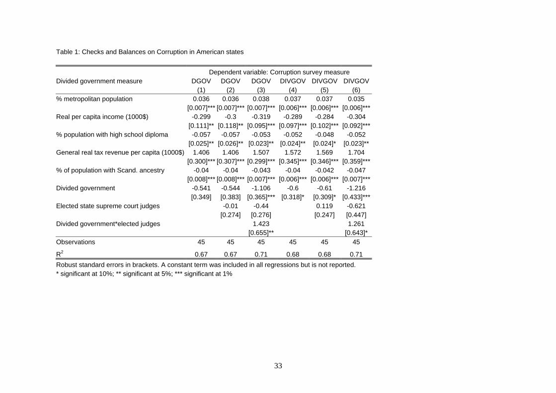
Table 1 presents the results of the main specification, for both measures of divided

government. The main explanatory variables are the share of the population residing in

metropolitan areas, income per capita, share of the population with at least a high school

diploma, state government tax revenue per capita, and share of population with Scandinavian

ancestry. Throughout the analysis, these variables have the expected signs and are strongly

significant.

To this specification, based – as mentioned above – largely on cross-country

work on the causes of corruption, we now add divided government (regressions (1) and (4)).

States in which different parties control the executive and legislative branches have

significantly lower corruption than states with unified government. The effect is slightly

larger and somewhat more precisely estimated when a governor facing a split legislature is

coded as divided government (regression (4), with the independent variable denoted divgov).

Our empirical estimates, hence, confirm the common intuition that divided government, or

shared power, contributes to a system of checks and balances which prevents the abuse of

power in public office. At the same time, then, it tentatively confirms our interpretation of the

PRT model, that is, that parties have an important role in making the system of checks and

balances work effectively.15

[Table 1 about here]

We now add an indicator variable for elected state Supreme Court judges

(regressions (2) and (5)), but find no direct effect of this variable. Do judicial selection

15 We cannot add anything to the interpretation of PRT of their model in terms of differences in separation of powers between presidential and parliamentary systems. Since our sample includes only presidential regimes, it is possible that the hypothetical case of parliamentary state governments would prove more corrupt than unified presidential state governments. Kunicová and Rose-Ackerman (2004), though, finds presidential regimes to be more corrupt than parliamentary ones on a comparative sample; see also Lassen (2007) who uses presidentialism as an instrument for corruption in an analysis of the size of the informal sector.

14

procedures, then, not affect the degree of corruption? Indeed, they might appear not to, since

we pointed out in the discussion above that having elected rather than appointed state

Supreme Court judges could affect corruption both positively and negatively. On the other

hand, remember that in our interpretation of the PRT model, the third branch of government

becomes important exactly when government, understood as the legislature and the executive

together, cannot control itself, which is the case under unified government. If that is the case,

we need to augment the specifications in (2) and (5) with an interaction term to allow for the

effect of the judiciary to be dependent on party control of government. This is done in

specifications (3) and (6).

Interacting divided partisan government and state Supreme Court selection

procedures produces a different result. While divided government continues to be significant,

we also find that states that elect rather than appoint Supreme Court judges have lower

corruption, though this is barely significant at conventional levels. The effect of elected or

accountable judges is particularly strong when government is unified, which is exactly when

government cannot or does not always control itself. Thus, in this case the judiciary provides

a check on the powers of the two other branches, as envisaged by Montesquieu. Conversely,

the judicial selection procedures are of less importance in the Lockean case with divided

government and thus no collusion among the branches, which is the case analysed by PRT.16

Again, the estimated checks and balances effects are largely the same across the two measures

of divided government.17 From these basic results we now extend the analysis in several

directions.

16 In Part II, we conjectured that judicial independence and divided government were substitutes. Thus, these specifications also imply that divided government has no effect when the judiciary is independent. 17 We also considered the possibility that the effect of different partisan configurations of divided government could matter for the impact of divided government on corruption. To do this we included separately indicator variables for Democratic governor vs. Republican legislature and Republican governor vs. Democratic

15

Judicial selection and partisan conflict

So far, we have analyzed the effects of elected vs. appointed state supreme courts as checks

on corruption in the other branches of government in an “institutional” way, in the sense that

we compare states using only the institutional selection procedure. We have not yet used

information on political leanings or party affiliations of state Supreme Court judges. This is

potentially important, as the same argument we made above for introducing parties into the

PRT model of separation of powers supports adding parties to the institutional state Supreme

Court argument. We believe the ability of courts to provide a check on other branches of

government can be diminished if the courts have preferences for -- or even run on -- the

platforms of particular parties. Indeed, the politicization of judicial selection that is often

associated with partisan elections is put forward by the so-called “court reformers” as a main

reason for switching to a hybrid plan (Hall, 2001). This line of argument echoes the early 20th

century Progressive movement, who argued for a switch from partisan to non-partisan judicial

elections. Nevertheless, Hall (2001) and Hall and Bonneau (2006) show that party politics,

measured by the degree of political competition, figures in all kinds of judicial elections,

whether directly partisan, non-partisan, or retention elections following initial appointment in

the hybrid plan.

To investigate whether the effectiveness of an elected court depends on partisan

factors, we divide states with direct elections into those where the Supreme Court is in

opposition to the other branches of government and those where this is not the case. We

follow the definition provided in the data description above. Thus, we code a state as having

“direct judicial elections in opposition” that, on average over the 1990s, had a majority of its

elected supreme court with a partisan affiliation or proclivity different from that of the

legislature. We cannot reject the null that the estimated coefficients are the same and, hence, continue to keep the non-partisan measure of divided government.

16

governor.18 Though the coefficients shift a little in offsetting ways, the overall estimated

effects do not depend on whether divided legislatures are treated as unified or divided

government. Results appear in Table 2.

[Table 2 here]

Consider the results in the second column, (6a). Estimates for basic control

variables and divided government are as before. Direct effects of elected, as opposed to

appointed, state supreme courts on corruption come from states whose supreme courts are in

partisan opposition to the government. The two estimates (across elected courts which are and

are not in opposition) are significantly different. Clearly, only elected courts in opposition

significantly dampen corruption. Furthermore, the interaction effects – which also are

significantly different – suggest that the effect of an elected judiciary on corruption is

strongest when it is in opposition to a unified government, confirming the institutional results

achieved above in the intuitively expected direction.

Selection vs. incentive effects

Hybrid selection schemes combine elements of appointment and elections. This allows us to

investigate the relative importance of the selection process, which is carried out in the

appointment procedure, and the effect of elections on accountability. Above, we coded hybrid

selection procedures as appointment. If we change this coding to elections, emphasizing the

retention vote rather than the appointment itself, we find that the effect of elected state

Supreme Court justices or, rather, the precision with which the effect is estimated, does

depend on the type of election (results not shown). If justices are directly elected, whether in

partisan or non-partisan elections, they provide a check on executive powers, and this effect is

18 We compare the average party affiliation for each state supreme court over the 1990s with the average partisanship of the governor in the same period. Alternatively, we could compute an opposition measure for each year and take the average; this makes no difference to the results.

17

significant as that found above. However, those justices who are first appointed but only later

subject to a retention vote appear not to have a similar effect on corruption. This does not

depend on whether we code supreme courts using only the institutional classification of Table

1 or the institutional-cum-partisan classification of Table 2.

This suggests that selection effects (cf. note 11) can be important when

considering the state supreme court’s role as a check on corruption in the other branches of

government. Besley and Payne (2006) found that incentive, rather than selection, effects were

the driving force in their results on worker discrimination cases. Hall (2001) found judges to

be held accountable for murder rate increases across different types of elections. In sum, these

results suggest that the relative importance of selection and incentive effects can depend on

the outcome under consideration.

V. Robustness of empirical results

We first note that we investigated the data for outliers. A test for outliers in the multivariate

sample including the interactions terms revealed three such cases, Minnesota and the Dakotas.

These three states are all outliers due to their high share of the population that have

Scandinavian ancestors. Indeed, if we re-analyze tables 1 and 2 dropping the three states, the

share of population with Scandinavian ancestors is now only marginally significant or

insignificant, but this exclusion has no effect on the other estimated coefficients.

To investigate further the robustness of the results, Table 3 introduces several

sets of control variables. We pay particular attention to variables found significant in earlier

work on corruption in US states (Alt and Lassen 2003). We check for other possible

influences on corruption to minimize the possibility that the effects of checks and balances

found above are due to spurious correlation, with divided government or judicial selection

procedures capturing the effects on corruption of other variables. We present only the

18

estimation results for the divgov variable, but these are indistinguishable from the results

obtained using the dgov measure, where split legislatures are coded as unified government.

[Table 3 here]

Only a few controls are significant: Southern states experience lower corruption as do states

with restrictions on campaign expenditures (see also Alt and Lassen, 2003), while we find less

precisely estimated effects in these specifications of open vs. closed primaries (though this is

significant when using the dgov measure), newspaper circulation,19 cable penetration shares,

term limits and initiative provisions (which are borderline significant when using the dgov

measure), and measures of political competition. Results on our main variables of interest

remain unaltered.

As an additional robustness check, we investigate our hypotheses using the data

on convictions for corruption described above instead of the survey measure. First, we

substitute the convictions data for 1999 for the survey measure in the cross-sectional

regression reported in Table 1. While the survey measure was missing for three mainland

states, the convictions data are available for all 48 states (but using the same 45 states as

above does not change the results below). The correlation between the survey measure and the

convictions data is .59. The results from a cross-sectional regression employing the

convictions data as the dependent variable, shown as regression (13) in Table 4, are identical

in terms of statistical significance to the results using the survey measure, though the actual

estimates cannot be readily compared due to the different dependent variables. This confirms

19 Sometimes denoted the fourth branch of government, an independent media exposes corruption (Adserà et al. 2003). In principle, the effects could be contingent on the partisanship of the media, if these could be measured.

19

that our findings using the survey data are not an artifact of this particular data set but in fact

carry over to other measures of corruption.20

We note one difference between the two cross sectional measures. It is that

consistently in the survey data, the effect of elected supreme courts arise at least as much in

partisan as in non-partisan elections (results not shown), while in the convictions data, the

cross sectional analysis (column 14) suggests that non-partisan elections are more important

for reducing corruption than partisan elections. Despite this caveat, to which we return below,

we believe that the results from the convictions data are consistent with the qualitative

outlines of the survey data.

[Table 4 here]

The remaining three columns show the results of panel data regressions,

controlling for state and year fixed effects. The set of controls is not exactly the same as in the

cross sectional analysis, for reasons of data availability. We did not have sufficient temporal

variation in metropolitan population and population share with Scandinavian ancestry to

include them here, but we include population size, as the correction for number of elected

officials may not be sufficient to capture size effects in the number of convictions (see the

discussion in Maxwell and Winters, 2005) and a time trend, as a number of variables, notably

divided government and corruption convictions, trend upward in the sample period. For

reasons of data availability, public sector expenditures are substituted for revenues.

Column (15) reports results from a standard panel data regression of the

convictions measure on divided government and control variables. As in the cross sectional

regressions, the presence of divided government is associated with a significantly lower level

of corruption, even if it is significant only at the 10 % level. State and year fixed effects are 20 Repeating the inclusion of additional controls from Table 3 using the convictions measure suggests that there are significantly lower conviction rates in states with high cable penetration rates and, marginally so, in states with provisions for direct voter initiatives.

20

strongly significant, as is the time trend, while the results on the controls generally fit the

pattern identified in the cross sectional analysis. The pattern of the year fixed effects is

interesting. Relative to the base year 1977, which is the first year for which data on

corruptions convictions are available, every year in the period 1983-1990, which almost

exactly coincides with the Republican administrations at the federal level, sees more

convictions for corruption, while the periods before and after, during the Democratic

administrations, are at the 1977 level. We return to this in the conclusion, below.21

As above, the results on Supreme Court judges (column 16) broadly follow the

cross-sectional results. There is very little variation between the groups of elected and

appointed judges over the period we consider, 22 and we estimate the direct effect of elected

judges on corruption to be negative, but only slightly larger than its standard error. The

interaction effect also has the expected sign, but this estimate lacks precision. The direct

effect of divided government is negative, bigger than in column (15), and continues to be

significant at the 10 % level.

Having more data allows us to investigate in more detail the separate effects of

partisan vs. non-partisan elections discussed above. The final column (17) reports results

when we distinguish supreme courts elected in partisan elections (omitted case here) from

those elected through non-partisan elections and appointed, respectively. In this case, we find

that supreme courts selected through non-partisan elections reduce corruption (p = .004),

compared to those selected through partisan elections. Divided government continues to be

significant, almost at the 5 % level, and, while not quite significant, the sign on the interaction

21 If we exclude the time trend, all years from 1983 and onwards have more convictions than 1977. Relative to 1977, the coefficients on the common year effects are stable or increase slightly until 1990, decline in the mid-1990s and increase again towards 1999, which is where our data ends. 22 Other studies looking at judicial selection procedures (Hanssen, 2004; Berkowitz and Clay, 2006; Besley and Payne, 2006) work with panels spanning back to 1950’s where much more frequent changes were taking place. See Berkowitz and Clay (2006) on the evolution of state Supreme Court institutions.

21

effect suggests that non-partisan courts work as an additional check on government when

government is unified. There is no remotely significant effect of appointed supreme courts

relative to courts elected in partisan elections. In addition, in results not reported, we could

identify no systematic effects of whether state supreme courts were controlled by the party in

(unified) government or not. One concern is that, even with panel data, our ability to

distinguish between partisan configurations for non-partisan and partisan elected judges may

be influenced by excluded controls. We return to this in future work.

The broad conclusion that emerges from these robustness checks is that divided

government reduces corruption, that having some form of elected judges probably reduces

corruption, and that the interaction effects suggest that divided government and elected judges

are substitutes in controlling corruption.

VI. Causality issues

Our interpretation of the empirical results so far has been that there is a causal effect of the

presence of divided government and judicial institutions on corruption. This is supported by

the historical accounts of Wallis (2004) and Glaeser and Goldin (2004) that institutional

response to the problem of corruption has been settled since the early twentieth century. Two

potential problems exist, however, with this explanation. First, the observed correlation could

be the result of reverse causality, that is, the causal effect may be that the presence of

corruption in state governments induces voters to choose unified governments in order to

lower corruption, or to push for judicial selection procedures different from direct partisan

elections, rather than divided government and selection procedures being the causes of lower

corruption.

A direct check of this reverse causality argument is to consider the effects of

lagged corruption on divided government. Unfortunately, no survey similar to the one

22

employed here exists for the 1980s, so we use the published figures on convictions for misuse

of public office (similar to the data we used for panel data analysis) used by Meier and

Holbrooke (1992). These were the first widely available data on corruption in American state

governments and might well have influenced informed public perception of corruption at the

state level. If we regress the presence of divided government in the 1990s on convictions data

from the 1980’s we find no effects even close to significant, regardless of the measure for

divided government, both in a univariate regression and controlling for all the other potential

determinants of divided governments discussed above. In any case, if the population in

corrupt states specifically elect different parties to control the two branches of government

with the aim of reducing corruption, the endogeneity bias on the estimate of the effect of

divided government on corruption would be towards zero. Thus, while endogeneity means

that our estimate may be too small, the finding that divided government reduces corruption

remains correct.

The second potential problem is that the demonstrated effects could simply be

spurious correlation caused by omitted third factors like a “culture of corruption” which in

turn is correlated with divided government and judicial selection procedures. When such

omitted variables are not controlled, the variables of interest could be correlated with the error

term of the regression leading to inconsistent empirical estimates. To the extent that such a

culture of corruption is fixed over time, the panel data evidence reported in table four suggests

that divided government continues to have an effect on corruption, while the evidence

regarding the judiciary is more mixed.

In the cross-sectional data, we believe the inclusion of the (highly significant)

share of the population reporting Scandinavian ancestors, while not perfect, goes some way

towards capturing a persistent (lack of ) tolerance for corruption (see Treisman, 2000, for

23

comparative evidence that Scandinavian countries have lower corruption, and Knack, 2002,

for effects of Scandinavian ancestry on measures of social capital in the US). We also

experimented with various state level measures of the strength of the Progressive movement

of the early twentieth century, which had combating corruption as a central agenda. These

measures were negatively related to corruption in the 1990’s, but were generally insignificant

and did not affect the estimates of the other variables’ effects on corruption in any way. The

wide range of potential controls considered above, and their small influence on the estimated

effects for the variables of interest considered here, also provides some reassurance that

spurious correlation is not the key reason for the observed results.

Finally, we also investigated the possibility of establishing causality by using

instrumental variables. If we could identify variables that affect the occurrence of divided

government and at the same time do not affect corruption, this would provide a stronger case

for a causal interpretation of the empirical findings. However, as is typical in empirical

analyses of the causes of corruption, identifying such instruments is difficult since most

candidate instruments have a potential direct influence on corruption. Consider one such

example: Fiorina (1994) argues that the increasing prevalence of divided state governments

can be attributed to the deterioration of Republican support in state legislatures. He explains

this in turn partly by the increasing professionalization of the legislatures, in terms of full-

time service and remuneration. This made legislative service relative more attractive to

Democratic candidates, who are argued to have less lucrative outside career opportunities than

Republican candidates.

We capture this effect by using as an instrument the average salary of state

legislators in the 1980’s. This is correlated with the occurrence of divided government in the

24

1990’s (di Tella and Fisman 2004), but may also be correlated directly with corruption.23 The

effect of salaries is insignificant and does not affect other results if included directly in the

regressions of Tables 1 and 2. However, IV-analysis using other potential (weak) instrumental

variables suggests that the inclusion of the salaries variable only in the first stage regression is

inappropriate, as it results in a rejection of a test for no overidentification. Similar problems

arise in the instrumentation of judicial selection procedures.24 In sum, though, our inability to

identify appropriate instruments does not imply that the effect we identify is not causal and,

for the reasons given above, we remain modestly confident for now that the observed

correlations can be given a causal interpretation.

VII. Discussion and Concluding Remarks

We find that divided government in American states is associated with lower corruption. This

confirms the popular perception of divided government as providing a system of checks and

balances between the executive and legislative branches. The finding emphasizes the role of

parties “on top” of institutions and, hence, provides, if indirectly, a qualification to Persson,

Roland and Tabellini’s (1997) discussion of parliamentary vs. presidential regimes and their

relationship with rent-seeking and corruption. Institutional separation of powers does not

always imply a functional separation of powers if institutional actors can collude, something

for which political parties provide a natural forum.

We also include the third branch of government, and find in the cross-sectional

data from the late 1990’s that having elected, rather than appointed, state supreme court

23 For example, this would be the case if higher pay (legal rent-seeking) reduced the demand for corruption (illegal rent-seeking). 24 As noted above, there are very few changes in judicial selection procedures over the period covered by our sample. Further, selection procedures, and changes therein, in the 1990’s are not correlated with convictions on corruption in the 1980’s. Hence, concerns about bias related to judicial selection procedures should be concentrated on omitted variables such as “judicial culture,” which may potentially be correlated with the selection procedures. In work on employment discrimination charges, Besley and Payne (2006) find no effects of instrumenting selection procedures.

25

judges is also associated with lower corruption and that divided government and elected

supreme court judges are substitutes in curbing corruption. This means that the effect of a

judiciary accountable to the public is stronger in states where the executive and legislative

branches of government are controlled by the same party. Using convictions data in a panel

context, we generally replicated these results, but found that the effect seems to be driven by

courts selected specifically in non-partisan elections.

Interestingly, the panel data also suggested temporal patterns in the number of

corruption convictions. While convictions for public corruption have been trending strongly

upwards during the last quarter of the 20th century, the years under a federal Republican

administration witnessed above-trend numbers of convictions. There are many possible

explanations for this pattern, including that there was simply more state level corruption under

the Republican administrations. However, as noted above, in practice the number of

convictions also reflects prosecutorial effort, as some state cases of corruption are prosecuted

at the federal level. As prosecutorial effort is not directly observable, this, to us, reinforces the

case for using both corruption perceptions surveys as well as convictions data when gauging

the level of corruption in American state governments.

Overall, the results accord with recent findings concerning the effects of the

judiciary on outcomes (Besley and Payne, 2006), but may contradict a long-standing belief in

the court reform literature (e.g. Hanssen, 2001) that appointed courts are more independent.25

Importantly, Besley and Payne (2006) observe that different notions of judicial independence

are at work. On the one hand, there is independence from the executive and legislature, which

is what is referred to as ”independence” in both the court reform and comparative literatures

25 We examined whether the effect of appointed courts depends on party congruence or opposition. Taking appointed courts with partisan congruence as the base case, in the cross sectional analysis, appointed courts in opposition does not affect corruption perceptions in the survey, but is weakly associated with lower corruption using the convictions data (p = .097).

26

(La Porta et al. 2004). This matters for the process of judicial review of laws affecting public

policies. In the context of American state courts, judicial independence to some also implies

independence from popular opinion (Baum, 2003). Appointed state Supreme Court judges are

independent from popular opinion and may, as noted by La Porta et al. (2004) and Glaeser

and Shleifer (2002) in a comparative context, therefore protect property rights to a larger

extent.

However, at the state level such courts may not be independent from either

business and other interest groups or the executive branch of government due to the bundling

of the political choice and judicial selection. This independence can be achieved by elected

courts, though at the risk of judges pandering more to public opinion, which may or may not

be desirable from a welfare point of view.26 Our results certainly are consistent with the view

that accountability and independence from the legislative and executive branches are

important for the judicial branch to provide a check on other branches of government so as to

ensure that these do not abuse their public office for private gain. However, our results on the

judiciary are only a first step towards an understanding of these mechanisms. Future research

should investigate in more detail the interdependence of different institutions in affecting the

quality of governance, and efforts could be made to create panels of corruption surveys in the

US as well as better and more detailed data for effective checks and balances in comparative

samples along the lines of La Porta et al. (2004).

26 See Brace and Boyea (2004) for an analysis of pandering by state supreme courts in the context of capital punishment.

27

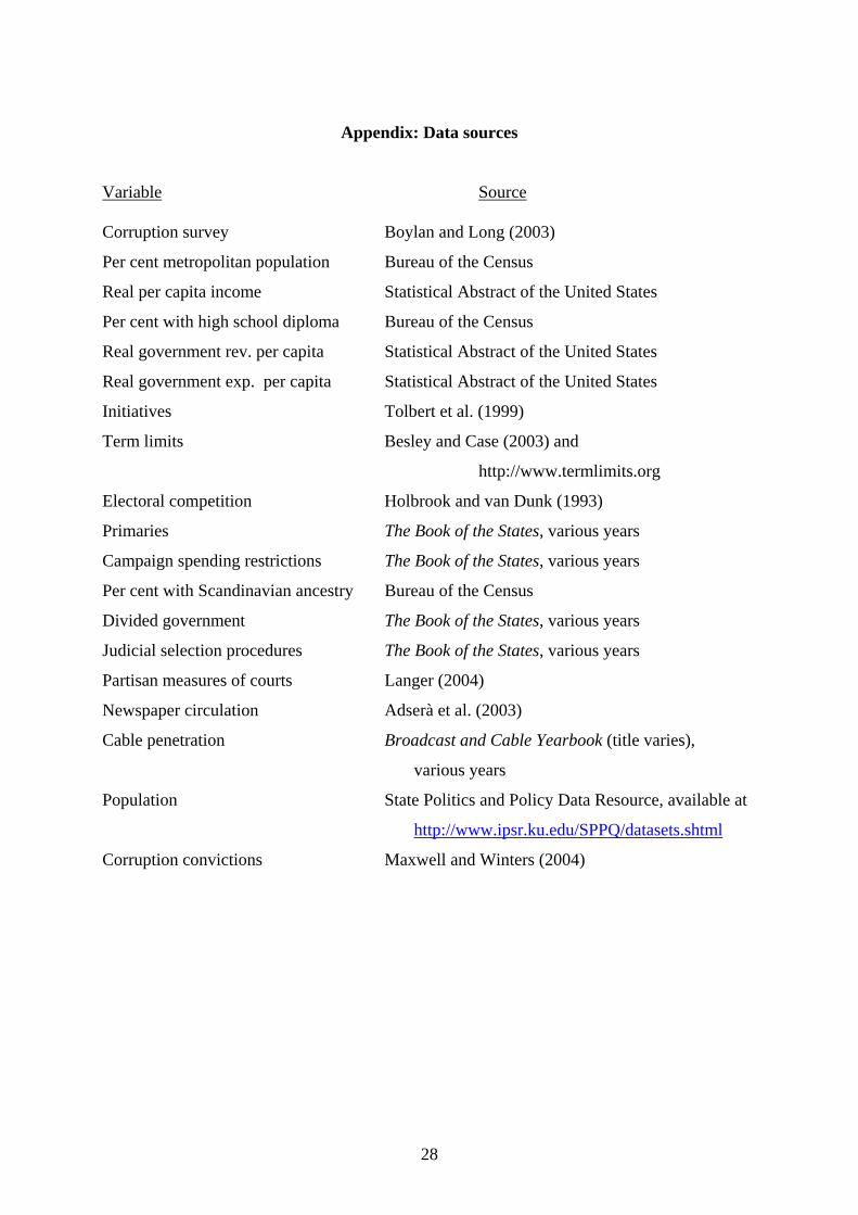
Appendix: Data sources Variable Source Corruption survey Boylan and Long (2003)

Per cent metropolitan population Bureau of the Census

Real per capita income Statistical Abstract of the United States

Per cent with high school diploma Bureau of the Census

Real government rev. per capita Statistical Abstract of the United States

Real government exp. per capita Statistical Abstract of the United States

Initiatives Tolbert et al. (1999)

Term limits Besley and Case (2003) and

http://www.termlimits.org

Electoral competition Holbrook and van Dunk (1993)

Primaries The Book of the States, various years

Campaign spending restrictions The Book of the States, various years

Per cent with Scandinavian ancestry Bureau of the Census

Divided government The Book of the States, various years

Judicial selection procedures The Book of the States, various years

Partisan measures of courts Langer (2004)

Newspaper circulation Adserà et al. (2003)

Cable penetration Broadcast and Cable Yearbook (title varies),

various years

Population State Politics and Policy Data Resource, available at

http://www.ipsr.ku.edu/SPPQ/datasets.shtml

Corruption convictions Maxwell and Winters (2004)

28

References Ades, A. and R. di Tella, 1999, Rents, competition, and corruption. American Economic

Review 89, 982-93.

Adserà, A., C. Boix, and M. Payne, 2003, Are you being served? Political accountability and

governmental performance. Journal of Law, Economics, and Organization 19, 445-490.

American Judicature Society, 2007. Website on Judicial Selection in the States.

http://www.ajs.org/js/ (accessed March 15, 2007).

Alt, J. E. and D. D. Lassen, 2003, The political economy of institutions and corruption in

American states. Journal of Theoretical Politics 15, 341-365.

Barro, R. J., 1973, The control of politicians. Public Choice 14, 19-42.

Baum, L., 2003, Judicial elections and judicial independence: The voter’s perspective. Ohio

State Law Journal 64(13).

Berkowitz, D. and K. Clay, 2006, The effect of judicial independence on courts: Evidence

from the American states. Journal of Legal Studies 35, 399-400.

Besley, T., 2006, Principled agents: The political economy of good government (Oxford,

Oxford University Press).

Besley, T. and A. Case, 2003, Political institutions and policy choices: Evidence from the

United States. Journal of Economic Literature 41, 7-73.

Besley, T. and S. Coate, 2003, Elected versus appointed regulators: Theory and evidence.

Journal of the European Economic Association 1, 1176-1206.

Besley, T. and A. Payne, 2006, Implementation of anti-discrimination policy:

Does judicial selection matter?” Manuscript, LSE and McMaster, May.

Boylan, R. T. and C. X. Long, 2003, Measuring public corruption in the American states: A

survey of state house reporters. State Politics and Policy Quarterly 3, 420-38.

Brace, P. and B. Boyea, 2004, State supreme court decision-making: A re-evaluation of the

electoral connection. Presented to the Annual Meeting of the American Political Science

Association, Chicago, September.

Brace, P., L. Langer and M. G. Hall, 2000, Measuring the preferences of state supreme court

judges. Journal of Politics 62, 387-413.

Brown, D. S., M. Touchton and A. B. Whitford, 2006, Political polarization as a constraint on

government: Evidence from corruption. Manuscript, available at SSRN:

http://ssrn.com/abstract=782845

29

di Tella, R. and R. Fisman, 2004, Are politicians really paid like bureaucrats?” Journal of

Law and Economics 47, 477-513.

Feld, L. P. and S. Voigt, 2003, Economic growth and judicial independence: Cross-country

evidence using a new set of indicators. European Journal of Political Economy 19, 497-

527.

Ferejohn, J., 1986, Incumbent performance and electoral control. Public Choice 50, 5-26.

Fiorina, M. P., 1994, Divided government in the American states: a Byproduct of legislative

professionalism?” American Political Science Review 88, 304-16.

Gerring, J. and S. C. Thacker, 2004, Political institutions and corruption: The role of

unitarism and parliamentarism. British Journal of Political Science 34, 295-330.

Glaeser, E. and C. Goldin, 2004, Corruption and reform: An introduction. NBER Working

Paper no. 10775, September.

Glaeser, E. and R. E. Saks, 2006, Corruption in America. Journal of Public Economics, 90,

1053-1072.

Glaeser, E. and A. Shleifer, 2002, Legal origins. Quarterly Journal of Economics 117, 1193-

1229.

Hall, M. G., 2001, State supreme courts in American democracy: Probing the myths of

judicial reform. American Political Science Review 95, 315-30.

Hall, M. G. and C. W. Bonneau, 2006, Does quality matter? Challengers in state Supreme

Court elections. American Journal of Political Science 50, 20-33.

Hanssen, F. A., 2001, Independent courts and administrative agencies: An empirical analysis

of the states. Journal of Law, Economics, and Organization 16, 534-71.

Hanssen, F. A., 2004, Is there a politically optimal level of judicial independence? American

Economic Review 94, 712-729.

Holbrook, T. and E. van Dunk, 1993, Electoral competition in the American states. American

Political Science Review 87, 955-962.

Knack, S., 2002, Social capital and the quality of government: Evidence from the U.S. States.

American Journal of Political Science 46, 772-785.

Kousser, Thad, 2005, Term limits and the dismantling of state legislative professionalism

(Cambridge: Cambridge University Press)

Kunicová, J. and S. Rose-Ackerman, 2005, Electoral rules as constraints on corruption.

British Journal of Political Science 35, 573-606.

30

Kunicová, J., 2006, Political corruption: Another peril of presidentialism?” California

Institute of Technology, working paper.

La Porta, R., F. Lopez-de-Silanes, C. Pop-Eleches and A. Shleifer, 2004, Judicial checks and

balances. Journal of Political Economy 112, 445-470.

Laffont, J.-J., 2001, Incentives and political economy (Oxford: Oxford University Press)

Langer, L., 2002. Judicial review in state Supreme Courts. (Albany: State University of NY

Press)

Langer, L., 2004. NSF CAREER Grant, SES-0092187 Multiple actors and competing risks in

the policymaking of judicial review. University of Arizona, accessed June 2005.

Lassen, D. D., 2007, Ethnic divisions, trust, and the size of the informal sector. Journal of

Economic Behavior and Organization, forthcoming.

Maskin, E. and J. Tirole, 2004, The politician and the judge. American Economic Review 94,

1034-1054.

Maxwell, A. and R. F. Winters, 2004, A quarter century of (data on) political corruption.

Presented to MPSA Meetings. Database available at

http://www.dartmouth.edu/~rwinters/Datasets.html (accessed March 15, 2007).

Maxwell, A. and R. F. Winters, 2005, Political corruption in America. Manuscript, Dartmouth

College, May.

Meier, K. J. and T. M. Holbrook, 1992, ‘I seen my opportunities and I took’em: Political

corruption in the American states. Journal of Politics 54, 135-155.

Montinola, G. and Richard J., 2002, Sources of corruption: A cross-country study. British

Journal of Political Science 32, 147-170.

Morgenstern, A., 2004, Separation of powers and party politics – on the value of divided

government. Presented to the Annual Meeting of the American Political Science

Association, Chicago, September.

Persson, T., G. Roland and G. Tabellini, 1997, Separation of powers and political

accountability. Quarterly Journal of Economics 112, 1163-1202.

Persson, T., G. Roland and G. Tabellini, 2000, Comparative politics and public finance.

Journal of Political Economy 108, 1121-1161.

Persson, T. and G. Tabellini, 1999, The size and scope of government: Comparative politics

with rational politicians. European Economic Review 43, 699-735.

31

32

Persson, T., G. Tabellini and F. Trebbi, 2003, Electoral rules and corruption. Journal of the

European Economic Association 1, 958-989.

Salzberger, E. M., 1993, A positive analysis of the doctrine of the separation of powers, or:

Why do we have an independent judiciary? International Review of Law and Economics

13, 349-379.

Schultz, C., 2005, Information, polarization and delegation in democracy. Manuscript,

University of Copenhagen.

Tolbert, C. J., D. H. Loewenstein and T. Donovan, 1999, Election law and rules for using

initiatives, in S. Bowler, T. Donovan and C. Tolbert, eds., Citizens as legislators: Direct

democracy in the United States (Columbus: Ohio State University Press).

Treisman, D., 2000, The causes of corruption: A cross-national survey. Journal of Public

Economics 76, 399-457.

Wallis, John J., 2004, The concept of systematic corruption in American political and

economic history. Presented to NBER conference on Reform and Corruption, July.

33

Table 1: Checks and Balances on Corruption in American states Dependent variable: Corruption survey measure Divided government measure DGOV DGOV DGOV DIVGOV DIVGOV DIVGOV (1) (2) (3) (4) (5) (6) % metropolitan population 0.036 0.036 0.038 0.037 0.037 0.035 [0.007]*** [0.007]*** [0.007]*** [0.006]*** [0.006]*** [0.006]***Real per capita income (1000$) -0.299 -0.3 -0.319 -0.289 -0.284 -0.304 [0.111]** [0.118]** [0.095]*** [0.097]*** [0.102]*** [0.092]***% population with high school diploma -0.057 -0.057 -0.053 -0.052 -0.048 -0.052 [0.025]** [0.026]** [0.023]** [0.024]** [0.024]* [0.023]**General real tax revenue per capita (1000$) 1.406 1.406 1.507 1.572 1.569 1.704 [0.300]*** [0.307]*** [0.299]*** [0.345]*** [0.346]*** [0.359]***% of population with Scand. ancestry -0.04 -0.04 -0.043 -0.04 -0.042 -0.047 [0.008]*** [0.008]*** [0.007]*** [0.006]*** [0.006]*** [0.007]***Divided government -0.541 -0.544 -1.106 -0.6 -0.61 -1.216 [0.349] [0.383] [0.365]*** [0.318]* [0.309]* [0.433]***Elected state supreme court judges -0.01 -0.44 0.119 -0.621 [0.274] [0.276] [0.247] [0.447] Divided government*elected judges 1.423 1.261 [0.655]** [0.643]* Observations 45 45 45 45 45 45

R2 0.67 0.67 0.71 0.68 0.68 0.71 Robust standard errors in brackets. A constant term was included in all regressions but is not reported. * significant at 10%; ** significant at 5%; *** significant at 1%

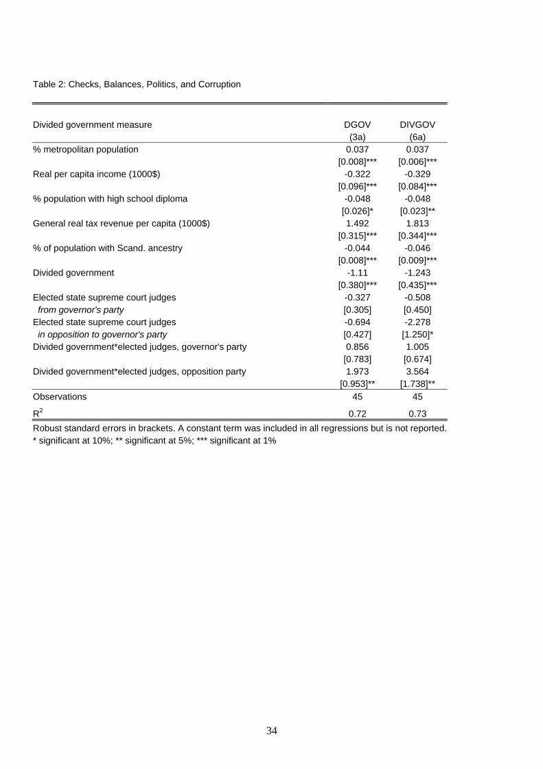
Table 2: Checks, Balances, Politics, and Corruption Divided government measure DGOV DIVGOV (3a) (6a) % metropolitan population 0.037 0.037 [0.008]*** [0.006]*** Real per capita income (1000$) -0.322 -0.329 [0.096]*** [0.084]*** % population with high school diploma -0.048 -0.048 [0.026]* [0.023]** General real tax revenue per capita (1000$) 1.492 1.813 [0.315]*** [0.344]*** % of population with Scand. ancestry -0.044 -0.046 [0.008]*** [0.009]*** Divided government -1.11 -1.243 [0.380]*** [0.435]*** Elected state supreme court judges -0.327 -0.508 from governor's party [0.305] [0.450] Elected state supreme court judges -0.694 -2.278 in opposition to governor's party [0.427] [1.250]* Divided government*elected judges, governor's party 0.856 1.005 [0.783] [0.674] Divided government*elected judges, opposition party 1.973 3.564 [0.953]** [1.738]** Observations 45 45

R2 0.72 0.73 Robust standard errors in brackets. A constant term was included in all regressions but is not reported. * significant at 10%; ** significant at 5%; *** significant at 1%

34

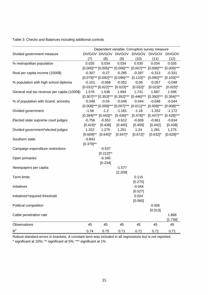
Table 3: Checks and Balances including additional controls Dependent variable: Corruption survey measure Divided government measure DIVGOV DIVGOV DIVGOV DIVGOV DIVGOV DIVGOV (7) (8) (9) (10) (11) (12) % metropolitan population 0.035 0.034 0.034 0.035 0.034 0.035 [0.005]*** [0.005]*** [0.006]*** [0.007]*** [0.006]*** [0.006]***Real per capita income (1000$) -0.307 -0.27 -0.285 -0.287 -0.313 -0.331 [0.079]*** [0.092]*** [0.096]*** [0.110]** [0.095]*** [0.103]***% population with high school diploma -0.101 -0.068 -0.052 -0.06 -0.057 -0.048 [0.031]*** [0.022]*** [0.023]** [0.032]* [0.023]** [0.025]* General real tax revenue per capita (1000$) 1.578 1.536 1.694 1.741 1.687 1.596 [0.307]*** [0.353]*** [0.352]*** [0.446]*** [0.350]*** [0.354]***% of population with Scand. ancestry -0.048 -0.04 -0.046 -0.044 -0.048 -0.044 [0.008]*** [0.009]*** [0.007]*** [0.011]*** [0.009]*** [0.008]***Divided government -1.56 -1.2 -1.181 -1.18 -1.252 -1.172 [0.394]*** [0.443]** [0.436]** [0.478]** [0.447]*** [0.428]***Elected state supreme court judges -0.756 -0.552 -0.612 -0.609 -0.661 -0.634 [0.419]* [0.436] [0.465] [0.459] [0.442] [0.438] Divided government*elected judges 1.322 1.275 1.251 1.24 1.281 1.275 [0.609]** [0.645]* [0.647]* [0.672]* [0.632]* [0.628]**Southern state -0.843 [0.379]** Campaign expenditure restrictions -0.537 [0.212]** Open primaries -0.345 [0.234] Newspapers per capita -1.577 [2.209] Term limits 0.115 [0.275] Initiatives -0.044 [0.527] Initiatives*required threshold 0.024 [0.060] Political competition 0.005 [0.013] Cable penetration rate 1.868 [1.739] Observations 45 45 45 45 45 45

R2 0.74 0.75 0.71 0.71 0.71 0.71 Robust standard errors in brackets. A constant term was included in all regressions but is not reported. * significant at 10%; ** significant at 5%; *** significant at 1%

35

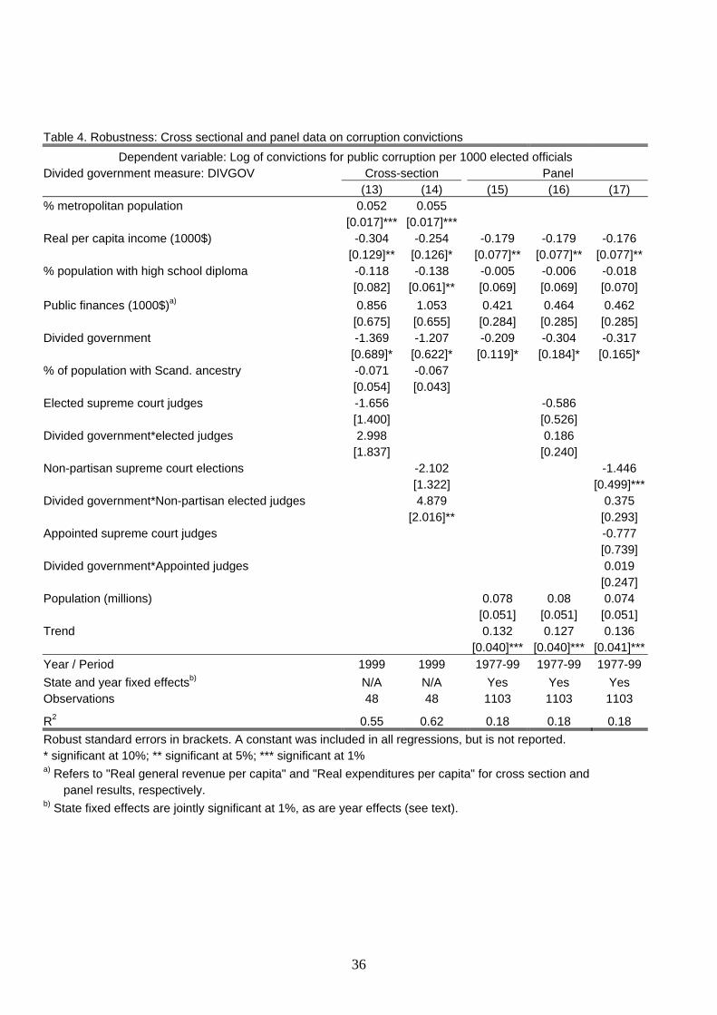
Table 4. Robustness: Cross sectional and panel data on corruption convictions Dependent variable: Log of convictions for public corruption per 1000 elected officials

Divided government measure: DIVGOV Cross-section Panel (13) (14) (15) (16) (17) % metropolitan population 0.052 0.055 [0.017]*** [0.017]*** Real per capita income (1000$) -0.304 -0.254 -0.179 -0.179 -0.176 [0.129]** [0.126]* [0.077]** [0.077]** [0.077]**% population with high school diploma -0.118 -0.138 -0.005 -0.006 -0.018 [0.082] [0.061]** [0.069] [0.069] [0.070] Public finances (1000$)a) 0.856 1.053 0.421 0.464 0.462 [0.675] [0.655] [0.284] [0.285] [0.285] Divided government -1.369 -1.207 -0.209 -0.304 -0.317 [0.689]* [0.622]* [0.119]* [0.184]* [0.165]* % of population with Scand. ancestry -0.071 -0.067 [0.054] [0.043] Elected supreme court judges -1.656 -0.586 [1.400] [0.526] Divided government*elected judges 2.998 0.186 [1.837] [0.240] Non-partisan supreme court elections -2.102 -1.446 [1.322] [0.499]***Divided government*Non-partisan elected judges 4.879 0.375 [2.016]** [0.293] Appointed supreme court judges -0.777 [0.739] Divided government*Appointed judges 0.019 [0.247] Population (millions) 0.078 0.08 0.074 [0.051] [0.051] [0.051] Trend 0.132 0.127 0.136 [0.040]*** [0.040]*** [0.041]***Year / Period 1999 1999 1977-99 1977-99 1977-99 State and year fixed effectsb) N/A N/A Yes Yes Yes Observations 48 48 1103 1103 1103

R2 0.55 0.62 0.18 0.18 0.18 Robust standard errors in brackets. A constant was included in all regressions, but is not reported. * significant at 10%; ** significant at 5%; *** significant at 1% a) Refers to "Real general revenue per capita" and "Real expenditures per capita" for cross section and panel results, respectively. b) State fixed effects are jointly significant at 1%, as are year effects (see text).

36