polyhedral analysis of up-peak traffic patterns in

Aalto University

School of Science

Degree Programme in Engineering Physics and Mathematics

Vesa Husgafvel

Polyhedral Analysis ofUp-peak Traffic Patterns inElevator Dispatching Problem

The document can be stored and made available to the public on the open internet

pages of Aalto University. All other rights are reserved.

Master’s ThesisEspoo, April 6, 2016

Supervisor: Professor Harri EhtamoAdvisor: Mirko Ruokokoski M.Sc. (Tech.)

Aalto UniversitySchool of ScienceDegree Programme in Engineering Physics and Mathematics

ABSTRACT OFMASTER’S THESIS

Author: Vesa Husgafvel

Title:Polyhedral Analysis of Up-peak Traffic Patterns in Elevator Dispatching Problem

Date: April 6, 2016 Pages: viii + 77

Major: Systems and Operations Research Code: Mat-2

Supervisor: Professor Harri Ehtamo

Advisor: Mirko Ruokokoski M.Sc. (Tech.)

Up-peak traffic is a common situation arising in elevator routing, where mostof the transportation requests given by passengers are directed from lower floorsto upper floors of a building. In this thesis, we examine three up-peak trafficpatterns that differ from each other with respect to the number of elevators orthe capacity of elevators. Analysis is based on a mixed-integer programmingformulation of the elevator dispatching problem (EDP).

Solutions of linear integer optimization problems span a convex hull, which iscalled a polytope. By examining the structure of a polytope, it is possible to findout special features of the problem to be studied. A central variable in descriptionof a polytope is dimension, which is defined as the number of affinely independentvectors contained in a polytope. In this work, we determine the dimension of eachup-peak traffic pattern polytope to be studied, or in the case we are not able togive an exact formula, we determine a lower and an upper bound for the value ofdimension. In addition, in each case we determine the number of feasible solutionsand the number of arcs in the reduced graph. Results relating to different patternsare compared with each other and with polyhedral results of similar optimizationproblems that appear in literature.

The obtained results of this work give new, fundamental knowledge of the polyhe-dral structure of up-peak traffic patterns - a subject that has not been previouslystudied. We believe that by combining our results with similar research results,e.g., polyhedral results of down-peak traffic patterns, our knowledge of the ele-vator dispatching problem deepens, which will help in designing of EDP solvingalgorithms.

Keywords: Elevator dispatching, elevator routing, integer optimization,up-peak traffic, polytope, polyhedral analysis

Language: English

ii

Aalto-yliopistoPerustieteiden korkeakouluTeknillisen fysiikan ja matematiikan koulutusohjelma

DIPLOMITYONTIIVISTELMA

Tekija: Vesa Husgafvel

Tyon nimi:Ylosruuhkamuodostelmien polyhedraalianalyysi hissien reititysongelmassa

Paivays: 6. huhtikuuta 2016 Sivumaara: viii + 77

Paaaine: Systeemi- ja operaatiotutkimus Koodi: Mat-2

Valvoja: Professori Harri Ehtamo

Ohjaaja: Diplomi-insinoori Mirko Ruokokoski

Ylosruuhka on yleinen hissien reitityksessa esiintyva tilanne, jossa suurin osa mat-kustajien antamista siirtokutsuista kohdistuu rakennuksen alemmista kerroksis-ta ylempiin kerroksiin. Tassa tyossa tutkitaan kolmea ylosruuhkamuodostelmaa,jotka eroavat toisistaan kaytettavissa olevien hissien lukumaaran tai hissien kapa-siteetin suhteen. Analyysi pohjautuu hissien reititysongelman (EDP) lineaariseensekalukuptimointiformulaatioon.

Lineaaristen kokonaislukuoptimointitehtavien ratkaisut virittavat konveksin kuo-ren, jota sanotaan tehtavan polytoopiksi. Polytoopin rakennetta tutkimalla onmahdollista selvittaa tarkasteltavan tehtavan erityispiirteita. Keskeinen polytoop-pia kuvaava suure on dimensio, joka maaritellaan polytoopin sisaltamien affiinistiriippumattomien vektorien lukumaarana. Tyossa maarataan kunkin tutkittavanylosruuhkamuodostelman polytoopin dimensio tai dimension arvolle maarataanala- ja ylaraja. Lisaksi kussakin tapauksessa maarataan kaypien ratkaisujen lu-kumaara seka kaarien lukumaara redusoidussa graafissa. Eri muodostelmiin liit-tyvia tuloksia vertaillaan seka keskenaan etta kirjallisuudessa esiintyvien saman-kaltaisten optimointiongelmien polyhedraalitulosten kanssa.

Tyossa saadut tulokset antavat uutta, perustavanlaatuista tietoaylosruuhkamuodostelmien polyhedraalirakenteesta - aiheesta jota ei ole ai-emmin tutkittu. On uskottavaa etta yhdistamalla saatuja tuloksia aiempientutkimustulosten (esim. alasruuhkamuodostelmia koskevien tulosten) kanssa,hissien reititysongelman tuntemus paranee, mika puolestaan edistaa ratkaisual-goritmien kehitysta.

Asiasanat: Hissien reititys, kokonaislukuoptimointi, ylosruuhka, poly-tooppi, polyhedraalianalyysi

Kieli: Englanti

iii

Acknowledgements

First and foremost, I wish to thank my instructor Mirko Ruokokoski and mysupervisor Professor Harri Ehtamo for their guidance and patience during thewriting process. Additionally, I am grateful to Kimmo Berg for his commentsand suggestions for improvements regarding this thesis. I also want to expressmy thanks to the Department of Mathematics and Systems Analysis forletting me to work there for most of the time of my studies: if I had not hadan opportunity to study alongisde my job, this Master’s thesis would not becompleted yet.

During my studies, a huge source of strength and happiness for me hasbeen my friends, who were always ready to listen to my worries and supportme whenever I had a hard time. I sincerely thank them, especially Maiju,for being my support all these years. Furthermore, special thanks go to myfellow student Ville for his constant willingness to solve my equations, fix mycode, but for also being a guy with whom I could enjoy a pint or two.

Finally, I would like to thank my family for supporting me through lifeand teaching me the values needed to succeed.

Espoo, April 6, 2016

Vesa Husgafvel

iv

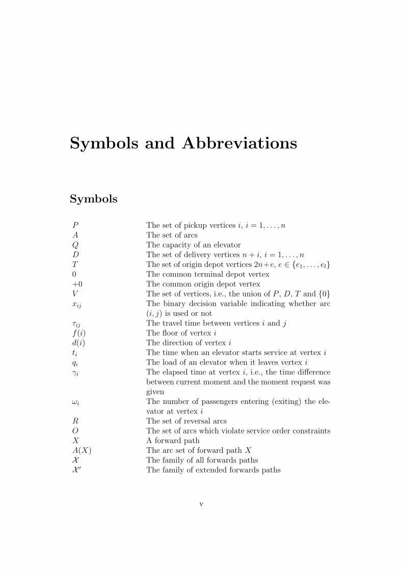
Symbols and Abbreviations

Symbols

P The set of pickup vertices i, i = 1, . . . , nA The set of arcsQ The capacity of an elevatorD The set of delivery vertices n+ i, i = 1, . . . , nT The set of origin depot vertices 2n+e, e ∈ e1, . . . , el0 The common terminal depot vertex+0 The common origin depot vertexV The set of vertices, i.e., the union of P , D, T and 0xij The binary decision variable indicating whether arc

(i, j) is used or notτij The travel time between vertices i and jf(i) The floor of vertex id(i) The direction of vertex iti The time when an elevator starts service at vertex iqi The load of an elevator when it leaves vertex iγi The elapsed time at vertex i, i.e., the time difference

between current moment and the moment request wasgiven

ωi The number of passengers entering (exiting) the ele-vator at vertex i

R The set of reversal arcsO The set of arcs which violate service order constraintsX A forward pathA(X) The arc set of forward path XX The family of all forwards pathsX ′ The family of extended forwards paths

v

EDPmn,l The up-peak traffic problem of n requests and l ele-

vators whose capacity is m. Shorter notation EDPmn

is used in the case l = nHmn,l The set of solutions to EDPm

n,l projected onto to thex-space

Gmn,l The reduced graph of EDPm

n,l

Amn,l The set of arcs in Gmn,l

PEDPmn,l

The polytope of EDPmn,l

PEDPmn,l|x The polytope of EDPm

n,l restricted to the x-space

D − EDP∞n The down-peak traffic problem of n requests and nelevators of infinite capacity

H∞D,n The set of solutions to D−EDP∞n projected onto thex-space

G∞D,n The reduced graph of D − EDP∞nA∞D,n The set of arcs in G∞D,nPD−EDP∞

nThe polytope of D − EDP∞n

Abbreviations

(S1, S2) (i, j) ∈ A : i ∈ S1, j ∈ S2(k, S) (i, j) ∈ A : i ∈ k, j ∈ Sx(S1, S2)

∑(i,j)∈(S1,S2)

xijΩ(S)

∑i∈S qi

|S| The cardinality of set SS V \ S

vi

Contents

Symbols and Abbreviations v

1 Introduction 11.1 Background . . . . . . . . . . . . . . . . . . . . . . . . . . . . 11.2 Objectives . . . . . . . . . . . . . . . . . . . . . . . . . . . . . 21.3 Structure . . . . . . . . . . . . . . . . . . . . . . . . . . . . . 3

2 Literature Review 42.1 Travelling Salesman Problem . . . . . . . . . . . . . . . . . . . 42.2 Vehicle Routing Problem . . . . . . . . . . . . . . . . . . . . . 52.3 Pickup and Delivery Problem . . . . . . . . . . . . . . . . . . 62.4 Elevator Dispatching Problem . . . . . . . . . . . . . . . . . . 6

3 Polyhedral and Graph Theory 93.1 Polyhedral Theory . . . . . . . . . . . . . . . . . . . . . . . . 93.2 Graph Theory . . . . . . . . . . . . . . . . . . . . . . . . . . . 133.3 Combinatorics . . . . . . . . . . . . . . . . . . . . . . . . . . . 14

3.3.1 Selections . . . . . . . . . . . . . . . . . . . . . . . . . 143.3.2 Principle of Inclusion and Exclusion . . . . . . . . . . . 173.3.3 Stirling, Bell, and Lah Numbers . . . . . . . . . . . . . 18

4 Integer Programming 224.1 Classification of Optimization Problems . . . . . . . . . . . . . 224.2 Relaxations . . . . . . . . . . . . . . . . . . . . . . . . . . . . 234.3 Modeling Techniques . . . . . . . . . . . . . . . . . . . . . . . 24

4.3.1 Related Variables . . . . . . . . . . . . . . . . . . . . . 244.3.2 Disjunctive Constraints . . . . . . . . . . . . . . . . . . 244.3.3 Degree and Subtour Elimination Constraints . . . . . . 254.3.4 Precedence Constraints . . . . . . . . . . . . . . . . . . 264.3.5 Strong Formulations . . . . . . . . . . . . . . . . . . . 27

4.4 Polyhedral Combinatorics in Integer Programming . . . . . . . 28

vii

4.4.1 Polyhedral Combinatorics in General . . . . . . . . . . 284.4.2 Symmetric Travelling Salesman Problem . . . . . . . . 294.4.3 Symmetric Travelling Salesman Problem with

Pickup and Delivery . . . . . . . . . . . . . . . . . . . 314.5 Integer Programming Algorithms . . . . . . . . . . . . . . . . 33

4.5.1 Simplex Algorithm . . . . . . . . . . . . . . . . . . . . 344.5.1.1 Basic Solutions . . . . . . . . . . . . . . . . . 344.5.1.2 Reduced Costs . . . . . . . . . . . . . . . . . 344.5.1.3 New Basic Solution . . . . . . . . . . . . . . . 354.5.1.4 Degeneracy . . . . . . . . . . . . . . . . . . . 364.5.1.5 Simplex Iteration . . . . . . . . . . . . . . . . 36

4.5.2 Branch and Bound Algorithm . . . . . . . . . . . . . . 374.5.2.1 Branch and Bound Iteration . . . . . . . . . . 38

4.5.3 Cutting Plane Method . . . . . . . . . . . . . . . . . . 384.5.3.1 Cutting Plane Iteration . . . . . . . . . . . . 39

5 Elevator Dispatching Problem (EDP) 405.1 Formulation . . . . . . . . . . . . . . . . . . . . . . . . . . . . 405.2 Polyhedral Analysis . . . . . . . . . . . . . . . . . . . . . . . . 45

6 EDP: Up-peak Traffic Pattern 496.1 General Assumptions . . . . . . . . . . . . . . . . . . . . . . . 496.2 Case 1: No Restrictions . . . . . . . . . . . . . . . . . . . . . . 51

6.2.1 Assumptions . . . . . . . . . . . . . . . . . . . . . . . . 516.2.2 Polyhedral Analysis . . . . . . . . . . . . . . . . . . . . 52

6.3 Case 2: Restricted Capacity . . . . . . . . . . . . . . . . . . . 556.3.1 Assumptions . . . . . . . . . . . . . . . . . . . . . . . . 556.3.2 Polyhedral Analysis . . . . . . . . . . . . . . . . . . . . 56

6.4 Case 3: Restricted Number of Elevators . . . . . . . . . . . . . 596.4.1 Assumptions . . . . . . . . . . . . . . . . . . . . . . . . 596.4.2 Polyhedral Analysis . . . . . . . . . . . . . . . . . . . . 60

7 EDP: Down-peak Traffic Pattern 657.1 Assumptions . . . . . . . . . . . . . . . . . . . . . . . . . . . . 657.2 Polyhedral Analysis . . . . . . . . . . . . . . . . . . . . . . . . 66

8 Conclusions 69

A Proof of LP cutTSPPD = LP sub

TSPPD 76

viii

Chapter 1

Introduction

1.1 Background

In modern times, when buildings are getting taller and taller, elevator routingis a problem that is increasingly gaining attention. For example, the tallestbuilding in the world, Burj Khalifa, located in Dubai, Arab Emirates, has aheight of 828 meters and contains 154 floors that incorporate 57 elevators:one can imagine how an inefficient elevator control system, in such a building,might lead to passengers’ extremely long journey or waiting times.

In the most basic form, an elevator group in a building consists of ca-pacitated single-deck elevators, such that each elevator shaft contains oneelevator. In high-rise buildings elevators are usually divided into groups andeach elevator group is controlled individually. Traditionally, a passenger callsan elevator at her arrival floor by pressing either an up or down button, in-dicating the desired direction of travel, after which she gives the destinationfloor inside the elevator. A more sophisticated alternative for calling anelevator is a destination control system, in which up and down buttons arereplaced with keypads. By using the keypad, a passenger makes a transporta-tion request by giving her destination floor to the device, before entering theelevator. After the transportation request is processed, the device guides thepassenger to the right elevator - by processing we refer to the time that ittakes from the control system to evaluate which elevator is optimal to servethis particular request. There is also a system where the serving elevator isannounced later, e.g., KL 118 in Kuala Lumpur, Malaysia. The time spenton processing should be short, typically less than half a second, because ifCPU time is long, the situation could have changed so much that the solutionis already outdated. In addition, it is uncomfortable for the passenger if shehas to wait for a long time before even knowing, which elevator is going to

1

CHAPTER 1. INTRODUCTION 2

serve her.Since new requests are received with varying time-intervals1, elevator

routing is also a dynamic problem. A common way to handle this kind of taskis to consider it as a snapshot problem: each moment defines a static problem,which is then solved whenever a new request arrives and/or a certain amountof time has passed. In addition to the dynamic nature of the problem, ele-vator routing contains a degree of stochasticity, since each (transportation)request can be viewed as a 3-dimensional random vector, whose componentsare arrival time, arrival floor, and destination floor of the request.

Elevator routing is a complicated task, which requires simultaneous fulfill-ment of several conditions in order to be efficient, practical, and comfortableway to transport people. Naturally, elevators have certain capacity restric-tions, and journey times of the passengers cannot be arbitrarily long butsome other constraints must be satisfied as well. For example, a commonprinciple is that passengers who are travelling upwards are not guided toelevators that are going downwards, and vice versa. Partially due to thecomplexity of the problem, it took a long time before a formulation in whichall constraints are given in exact mathematical form, was presented in [28]by Ruokokoski et al. In Ruokokoski et al. [29] computational experimentsare performed to demonstrate the goodness of this formulation compared totraditional methods that use collective control principle together with otherheuristic rules.

1.2 Objectives

In this paper, we define the elevator dispatching problem (EDP) and, basedon [28], formulate it as a snapshot mixed integer linear program. The readerswho are not yet familiar with the terminology, a mixed integer linear programrefers to an optimization problem in which objective function and constraintsare given in a linear form, such that some of the decision variables are re-quired to be integers. In our formulation, we assume that the elevators areadministered by a destination control system, and that each elevator shaftcontains only one single-deck elevator. Furthermore, the stochastic nature ofthe problem will not be considered.

Linear constraints of the EDP formulation form a structure called a poly-tope. The main purpose of this paper is to analyze this polytope and itsproperties. Due to the complexity of the problem, the structure of the poly-tope is very challenging to study, so most of the analysis is restricted to twospecial cases, an up-peak traffic pattern and a down-peak traffic pattern. An

1Alexandris [1] showed that arrival process follows a Poisson process.

CHAPTER 1. INTRODUCTION 3

up-peak traffic pattern is a situation in which most or all of the passengerstravel from the lobby to the upper floors of the building; down-peak trafficis the opposite situation. A typical example of up-peak traffic is the morn-ing peak, when people come to work and they must travel upwards in orderto get to their offices; similarly, at the end of the day, a down-peak occurswhen people are travelling to the lobby to exit the building. Ruokokoski etal. [28] presented some polyhedral results of one down-peak traffic pattern,but the polyhedral structure of up-peak traffic patterns has not earlier beenstudied at all. Our aim is to fill in this gap by studying separately three up-peak traffic patterns, where each pattern arises from a different assumptionon the number of elevators or their capacity. Although up-peak and down-peak traffic patterns are more or less opposite situations, their polyhedralstructures are surprisingly different. In order to see these differences, we alsopresent the main polyhedral results of the down-peak traffic pattern studiedby Ruokokoski et al. [28].

1.3 Structure

The rest of this thesis is structured as follows: in Chapter 2 we conducta short literature review in the elevator dispatching problem and introducesome other integer programming problems that are strongly related to el-evator routing. In Chapter 3 we present the main concepts of polyhedraland graph theory and derive some combinatorial results that are needed inlater chapters. Chapter 4 considers linear and integer linear programmingon a general level: we talk about relaxations, modeling techniques, and therole of polyhedral combinatorics in the field of our study. In that chapter,we also describe some of the most common integer programming algorithms.Chapters 5, 6, and 7 focus entirely on the elevator dispatching problem. Thenotation of the chapters relating to the EDP is tried to kept as similar aspossible as that in [28]. Chapter 8 summarizes the main results of our study.

Chapter 2

Literature Review

2.1 Travelling Salesman Problem

One of the most studied problems in the field of optimization is the travellingsalesman problem (TSP). In the TSP, a salesman must travel through a listof cities such that each city gets visited exactly once, and finally return tothe origin city. The question is, which route minimizes the travelling costs.Although the problem is simple to describe, it is very difficult to solve.

The origins of the TSP are not known, but the first mathematical formu-lation was presented by W.R. Hamilton and Thomas Kirkman in the 1800s.In the 1950s, the problem grew in popularity among scientific circles, whenGeorge Dantzig, Delbert Ray Fulkerson, and Selmer M. Johnson expressedthe TSP as an integer linear program and solved a large instance of theproblem at that time by using the cutting plane method [8]. 1

Many different forms of the TSP have been studied during the decades.In the symmetric travelling salesman problem (sTSP) the travelling costsbetween each two cities are the same regardless the direction of travel. Incontrast, in the asymmetric travelling salesman problem (aTSP), the trav-elling cost depends on the direction, which is often the situation when weconsider the prices of flight tickets. If more than one salesman can visit cities,the problem is known as multi travelling salesman problem (mTSP). In themTSP we can, e.g., set a minimum or maximum number of cities, in whichone salesman can visit. A comprehensive presentation of different TSP vari-ations can be found in the work ”The Traveling Salesman Problem and ItsVariations” [14].

1The cutting plane method is introduced in Section 4.5.

4

CHAPTER 2. LITERATURE REVIEW 5

2.2 Vehicle Routing Problem

The vehicle routing problem (VRP) is a generalization of the TSP with thefollowing setup: there are a number of vehicles available, which must delivergoods to a list of customers, each of them having a certain demand. Thegoods to be delivered are assumed to be of the same product. By requiringthat each vehicle must start and end their route at a depot, the objectiveis to find a set of routes satisfying customers’ demands, such that the totalroute cost is minimized. It is also usually assumed that splitting a customer’sdelivery is not possible, i.e., each customer must be visited by exactly onevehicle. The first VRP formulation was made by Dantzig and Ramser [9] inorder to optimize the costs of petrol deliveries.

The problem described above is the VRP in its very basic form. As in thecase of the TSP, there are numerous variations of the VRP and no consensusexists how to classify them. Pisinger and Ropke [26] propose a classificationinto five different categories:

1. Vehicle routing problem with time windows (VRPTW). In this variantthe customers are associated with time windows within which the visitsmust be made. A typical example of the VRPTW is pizza delivery, inwhich the maximum delivery time is often fixed to 30-60 minutes.

2. Capacitated vehicle routing problem (CVRP). In the CVRP each ve-hicle has limited capacity. Some CVRPs can also have restrictionsrelating to route lenghts or route durations.

3. Multi-depot vehicle routing problem (MDVRP). The MDVRP containsmultiple depots from which vehicles can start their routes.

4. Site-dependent vehicle routing problem (SDVRP). In this variant it isstipulated that certain customers can only be served by certain vehicles.

5. Open vehicle routing problem (OVRP). In the OVRP it is not requiredthat vehicles must return to the depot.

The TSP and VRP are similar problems, but the latter incorporates a widervariety of problems; indeed, the VRP of m uncapacitated vehicles can beidentified with the mTSP. In certain fields, such as in the logistics industry,transportation optimization can significantly lower the total costs, and as aresult, the VRP has been a hot research topic for the past 50 years. Liter-ature reviews on the VRP have been conducted, inter alia, by Laporte andNorbert [20] and Laporte and Osman [21]. The recent developments andpublications regarding the subject are covered by Kumar and Panneerseel-vam [19].


2.3 Pickup and Delivery Problem

In the vehicle routing problem it was assumed that vehicles start their routesfrom the depot, after which they can deliver the goods by driving straightto the customers. If the goods to be delivered are not in stock, it requiresthat vehicles must first leave the depot, pick up the goods from somewhere,and then drive back to the depot before the VRP model can be applied. Insuch cases, it would be more efficient if the goods could be delivered to thecustomers straight from the pickup places.

In the pickup and delivery problem (PDP) each transportation requestcomprises a pickup place and a destination: a vehicle must first pick up thegoods and then drive them to the destination. We require that vehicles muststart and end their routes at the depot. The VRP can be considered asa special case of the PDP, in which all pickup places locate at the depot.The objective in the PDP is to divide the transportation requests betweenvehicles so that the total costs will be minimized.

As in the case of the TSP and the VRP, there are also several extensionsfor the PDP. E.g., Savelsberg and Sol [30] presented the general pickup anddelivery problem (GPDP), which consists of a set of depots and allows thevehicles to start or end their routes at any of them. Cortes et al. [6] in-troduced and formulated another variant known as the pickup and deliveryproblem with transfers (PDPT), in which transferring loads between vehiclesis allowed. In the case when the ”goods” to be delivered are people, the PDPis called the dial-a-ride problem (DARP). The DARPs usually incorporaterestrictions on the passengers pickup and delivery times. Additionally, thetransportation time of a single passenger is required to stay below a certainmaximum limit. A typical example of the DARP is a door-to-door trans-portation of elderly or disabled people.

2.4 Elevator Dispatching Problem

The elevator dispatching problem (EDP) is a dial-a-ride problem, in whicha set of passengers have to be picked up from their arrival floors and trans-ported to their destination floors, so that a given objective function is mini-mized and a set of constraints are satisfied. Usually, these constraints relateto travel time, capacity of elevators and service order of passengers. Theirpoint is to guarantee that all passengers are delivered to their destinationfloors as efficiently as possible.

Different forms of the EDP appear in the literature, although elevatorrouting has historically gained relatively little attention compared to other


similar problems, such as the VRP. Elevator routing that is based on a des-tination control system, is one of the most common variants and also thevariant, which we chose for our study. Routing an elevator in a conventionalsystem is difficult as the destinations of passengers are not known in advance.In addition to Ruokokoski et al. [28, 29], destination control systems havebeen studied by, e.g., Koehler and Ottiger [18] and Tanaka et al. [33].

In some works relating to the EDP it has been assumed that elevatorshafts contain more than one car per shaft. If the cars are attached together,passengers at consecutive floors can be served simultaneously, and if the carsare separate, they can move independently as long as collisions are avoided.The former case is known as the multi-deck EDP[16, 32] and the latter asthe multi-car EDP [17].

In terms of solving the EDP, most of the research is based on heuris-tic methods such as artificial intelligence [31], neural networks [23], or localsearch [22], whereas exact algorithms have been considered only in few ar-ticles [15, 28, 33]. The reason for popularity of heuristic methods is due tothe complexity of the EDP, the real-time requirement that requests must beresponded very quickly but also the lack of a proper mathematical formu-lation: as mentioned in Chapter 1, the first - and so far only - a completemathematical formulation for the EDP is provided by Ruokokoski et al. [28].

The relationship between the TSP, VRP, PDP, DARP, and EDP is illus-trated in Figure 2.1.


PDP

TSP

V RP

DARP

EDP

Figure 2.1: A Venn diagram representing the relationship between the TSP,VRP, PDP, DARP, and EDP, where each class refers to the problem in itsbasic form.

Chapter 3

Polyhedral and Graph Theory

3.1 Polyhedral Theory

A linear combination of vectors xi ∈ Rn, i = 1, . . . ,m, is a weighted sum

λ1x1 + · · ·+ λmxm, (3.1)

where λi ∈ R, i = 1, . . . ,m. If∑m

i=1 λi = 1, the linear combination is calledaffine. A set S is affine if for each x,y ∈ S, it follows that λx+(1−λ)y ∈ S.From this definition it follows that affine sets are either lines or (hyper)planes.The set of all affine combinations of elements of S ⊂ Rn form the affine hullof S, which is denoted by aff(S). Clearly, for any affine set S, aff(S) = S.

A set of vectors x1, . . . ,xm is called linearly independent, if none of thevectors can be represented as a linear combination of others. Formally,

λ1x1 + · · ·+ λmxm = 0⇒ λi = 0 ∀i = 1, . . . ,m. (3.2)

Vectors x0,x1, . . . ,xm are affinely independent if x1 − x0, . . . ,xm − x0 arelinearly independent. Linearly independent vectors are always affinely inde-pendent, but (in general) not vice versa. If S is a set, which contains k + 1but not k + 2 affinely independent vectors, we say that the dimension of S,dim(S), is k.

When the linear combination (3.1) satisfies conditions∑m

i=1 λi = 1 andλi ≥ 0, ∀i ∈ 1, . . . ,m, it is called a convex combination. A set S is convexif for each x,y ∈ S, and λ ∈ [0, 1], it follows that λx + (1 − λ)y ∈ S. Allpoints in a convex set can be represented as a convex combination of theother points. Geometrically convexity means that the segment joining anytwo points of a convex set lies entirely within that set. The convex hull ofan set S, conv(S), is the smallest convex set containing S. If S is convex,conv(S) = S.

9

CHAPTER 3. POLYHEDRAL AND GRAPH THEORY 10

Convexity plays a central role in linear optimization problems, in whichthe feasible region of solutions is always of the same form: it consists of theintersection of finitely many hyperplanes. Let us give the following definition.

Definition 1. A set P ⊂ Rn is a polyhedron if it can be represented as theintersection of finitely many half-spaces, i.e.

P = x ∈ Rn|Ax ≤ b ,A ∈ Rm×n,b ∈ Rm (3.3)

If a polyhedron is bounded, meaning that it fits inside a ball of finiteradius, then the polyhedron is called a polytope1 From the point of viewof this study, all interesting polyhedra are bounded, and for this reason,forthcoming definitions will be based on polytopes. It is relatively easy toshow that each polytope is a convex set [3]. A less trivial fact relates to the”corners” of a polytope. In order to state this result, we first need to define,what a corner means.

Definition 2. Let P be a polytope. A vector x ∈ P is an extreme point ofP if there are no vectors y, z ∈ P , y, z 6= x, and a scalar λ ∈ [0, 1], such thatx = λy + (1− λ)z.

Next result shows that a polytope is uniquely determined by its extremepoints.

Theorem 1. Let X be the set of extreme points of a non-empty polytopeP . Then conv(X) = P .

Proof. See [3].

If all the extreme points of P are integers, we say that P is an integralpolytope. If the extreme points are binary valued, P is a 0-1-polytope.

A polytope comprises elements of different dimensionality. To see, whatthis means, consider a polytope P defined by (3.3). A valid inequality for Pis a linear inequality d′x ≤ e, where d, e ∈ Rn, if all points of P satisfy thatinequality. A valid inequality d′x ≤ e is supporting if for some point x0 ∈ Pit holds d′x0 = e. A set F ⊂ P whose points satisfy this equality, i.e.,

F = x ∈ P |d′x0 = e, (3.4)

is called a face of P ; we say that F is induced by the supporting inequalityd′x ≤ e. One should note that P itself is a face of P , because 0′x ≤ 0 is asupporting inequality for any polytope. A 0-dimensional face of P is called a

1A reader should note that different definitions of a polytope appear in literature. Inthis work, we stick with the given definition.


vertex, whereas a 1-dimensional face is known as an edge. Suppose now thatP is a k-polytope, i.e., the dimension of P is k. Then a (k − 1)-dimensionalface, (k − 1)-face, is called a facet.

An inequality a′ix ≤ bi in the system Ax ≤ b is called an implicit equalityif all feasible solutions of Ax ≤ b satisfy a′ix = bi. The subsystem ofall implicit equalities is denoted by (A=,b=). The rank of A=, rank(A=),indicates the number of linearly independent rows or columns in A=. Nexttheorem shows how dim(P ) depends on the implicit equalities of P .

Theorem 2. Let P = x ∈ Rn|Ax ≤ b be a non-empty polyhedron. Then

dim(P ) = n− rank(A=) (3.5)

Proof. See [7].

When A is large in size, it may be difficult to determine or even estimatethe dimension of P just by trying to find as many affinely independent solu-tions as possible. All implicit equalities are not usually known, so calculatingrank(A=,b=) is not possible either. We can, however, create a subsystemof (A=,b=), say (A=

S ,b=S ), by choosing all known implicit equalities. Since

(A=S ,b

=S ) ⊂ (A=,b=), it holds that rank(A=

S ) ≤ rank(A=). Now by usingTheorem 2, one gets an upper bound for the dimension of P :

dim(P ) ≤ n− rank(A=S ) (3.6)

If we can now find n − rank(A=S ) + 1 affinely independent solutions for P ,

the obtained upper bound is strict. Unfortunately, showing a set of vectorsaffinely or linearly independent is very difficult in general. For this reason,the proving is often based on the specific structure of the constraint matrixto be studied. In our study, the following proposition is found useful:

Proposition 1. Let x1, . . . ,xm be a set of n−vectors, n ≥ m, and de-note the ith entry of xj by xji . If there exists a sequence of ordered pairs(i1, j1), . . . , (im, jm), ik ∈ 1, . . . , n, jk ∈ 1, . . . ,m such that for eachk = 1, . . . ,m

1) xjkik 6= 0, and

2) xjik = 0 ∀j /∈ j1, . . . , jk,then x1, . . . ,xm are linearly independent.


Proof. It is obvious that if xj1 , . . . ,xjm are linearly independent, thenx1, . . . ,xm are also linearly independent. Consider a linear combinationλ1x

j1 + · · ·+ λmxjm for which it holds that∑m

k=1 λkxjk = 0. Now,( m∑

k=1

λkxjk

)i=i1

=m∑k=1

λkxjki1

= λ1xj1i1

+m∑k=2

λk xjki1︸︷︷︸=0 by 2)

= λ1xj1i1

= 0.

But since xj1i1 6= 0 by the first assumption, λ1 must be 0. Similarly,( m∑k=1

λkxjk

)i=i2

=m∑k=1

λkxjki2

= λ1xj1i2

+ λ2xj2i2

+m∑k=2

λkxjki2

= λ2xj2i2

= 0

implies that λ2 = 0. By continuing the process, one obtains λ1 = · · · = λm =0, which shows that xj1 , . . . ,xjm are linearly independent.

For example, if a matrix is defined by

A =

0 1 2 30 1 2 04 1 2 30 1 0 0

,we can show that its columns are linearly independent by choosing (i1, j1) =(4, 2), (i2, j2) = (2, 3), (i3, j3) = (1, 4), (i4, j4) = (3, 1), and then applyingProposition 1. Another useful way to determine the rank of a matrix is givenby Proposition 2.

Proposition 2. Let Ax = b be a system of linear equations a′ix = bi, whereA ∈ Rm×n, x ∈ Rn, b ∈ Rm, and n > m. If Ax = b has a solution, andthere exists vectors xi ∈ Rn, i = 1, . . . ,m, such that a′kx

i = bk ∀k 6= i buta′ix

i 6= bi, then rank(A) = m.

Proof. We show first that vectors [a′i,−bi], i = 1, . . . ,m, are linearly indepen-dent. Assume, by contradiction, that this is not true, in which case one of thevectors can be represented as a linear combination of the others. Formally,for some k ∈ 1, . . . ,m ∃ λ ∈ Rm−1 such that

[a′k,−bk] =∑

i∈1,...,m:i 6=k

[a′i,−bi]λi.


By taking the dot product with a vector [xk′, 1], we obtain

[a′k,−bk] · [xk′, 1] =

∑i∈1,...,m:i 6=k

[a′i,−bi] · [xk′, 1]λi

⇔ a′kxk − bk =

∑i∈1,...,m:i 6=k

(a′ixk − bi︸︷︷︸=0

)λi = 0

⇔ a′kxk = bk,

which is a contradiction. Hence, [a′i,−bi], i = 1, . . . ,m, are linearly indepen-dent and rank([A,−b]) = m. But since Ax = b has a solution, vector b canbe represented as a linear combination of the columns of A, in which caserank([A,−b]) = rank(A) = m, and the claim follows.

3.2 Graph Theory

A directed graph, or simply a digraph, G = (V,A) is an ordered pair, whereV is a set of vertices and A is a set of arcs that are ordered pairs of elementsof V . An arc between vertices i and j is denoted by (i, j). If arcs are definedas unordered pairs of V , then G is called an undirected graph. In such a casewe talk about edges instead of arcs, and they are denoted by E. An edgebetween vertices i and j is denoted by i, j. A loop is an arc, which connectsa vertex to itself, i.e., a pair containing the same element twice. If a graphcontains no loops it is called a simple graph. A simple undirected graph inwhich every pair of distinct vertices is connected by a unique arc is called acomplete undirected graph. A complete digraph is defined similarly with theexception that it contains a unique pair of arcs for each pair of vertices, onefor both directions.

A walk in a graph is a sequence (v0, a1, v1, a2, . . . , an, vn), where ai, i =1, . . . , n, is an arc connecting vi−1 and vi, respectively. If v0 = vn, then thewalk is called a cycle. A graph which contains no cycles is an acyclic graph.A walk is called a path if all its vertices are distinct; a walk is called a trail ifall its arcs are distinct. If the first and the last vertices are the same, but allother vertices are distinct, then a walk is a closed path, which is also knownas a circuit. If each vertex pair (vi−1, vi), i = 1, . . . , n, of a path is connectedby a unique arc in the underlying graph, then the path can be denoted by ashorter notion (v0, v1, . . . , vn) without the possibility of a misunderstanding.A graph is connected if for any v, q ∈ V there is an undirected walk fromv to q, i.e. a walk in which the directions of arcs are ignored. If there is awalk between each pair of vertices, then the graph is strongly connected. An


acyclic connected, undirected graph is a tree. Different graphs are illustratedin Figure 3.1.

Given a directed graph G = (V,A) and a set S ⊂ V , the cutset of S,δ(S), contains arcs whose one endpoint belongs to S and the other one to S.Formally,

δ(S) =

(i, j) ∈ A|i ∈ S, j /∈ S or i /∈ S, j ∈ S. (3.7)

The set of arcs whose both endpoints lie in S is denoted by ρ(S), i.e.,

ρ(S) =

(i, j) ∈ A|i, j ∈ S. (3.8)

These sets are also well-defined when G is an undirected graph: one simplyneeds to replace (i, j) with i, j.

Denote the vertex set of G by v(G) and the arc set by α(G). A graphH is a subgraph of G if v(H) ⊂ v(G) and α(H) ⊂ α(G). We say that His a vertex-induced subgraph of G if v(H) ⊂ v(G) and H contains all thearcs of G whose both endpoints are in H, i.e. α(H) = (i, j) ∈ α(G)|i ∈v(H), j ∈ v(H). Similarly, H is an arc-induced subgraph if α(H) ⊂ α(G)and H contains all the vertices, which are the endpoints of the arc set α(H),i.e. v(H) = i ∈ v(G)|α(H) ⊂ (i, v(G)) ∪ (v(G), i).

3.3 Combinatorics

3.3.1 Selections

The fundamentals of combinatorics relate to the question in how many waysk objects can be selected from a set of n objects. To answer this questionproperly, we must first define whether the order in which the objects areselected is significant or not, and can the same object be selected more thanonce. This leaves four cases to consider:

1. Order not significant and repetitions not allowed. Such a selection iscalled a k-combination of an n-set.

2. Order not significant and repetitions allowed. Such a selection is calleda k-multicombination of an n-set.

3. Order significant and repetitions not allowed. Such a selection is calleda k-permutation of an n-set.

4. Order significant and repetitions allowed. Such a selection is called ak-tuple of an n-set.


4

5

1

2

3

(a) A simple connected, undirectedgraph

4

5

1

2

3

(b) A simple disconnected digraph

4

5

1

2

3

(c) A tree

4

5

1

2

3

(d) A strongly connected graph

Figure 3.1: Four different graphs defined over same vertex setV = 1, . . . , 5.


The next theorem answers our question in all four cases.

Theorem 3.

1. The number of k-combinations of an n-set is(nk

):= n!

k!(n−k)! ,

where n! = n ∗ (n− 1) ∗ · · · ∗ 2 ∗ 1 is the factorial of n.

2. The number of k-multicombinations of an n-set is(n+k−1

k

).

3. The number of k-permutations of an n-set is n!(n−k)! .

4. The number of k-tuples of an n-set is nk.

Proof. We prove the claims in order 4, 3, 1, and 2. The claim number 4is obvious because the first object can be selected in n ways, the secondobject can also be selected in n ways etc., leaving the number of k-tuples asn ∗ · · · ∗ n︸︷︷︸

k times

= nk. When repetitions are not allowed but the order is significant,

the first object can be selected in n ways, the second object in n − 1 ways,and the kth object in n−(k−1) ways. Hence, the number of k-permutationsis n ∗ (n − 1) ∗ · · · ∗ (n − (k − 1)) = n!/(n − k)!. Since selected k objectsarise from k! different orders, the number of k-combinations is obtained bydividing the number of k-permutations by k!.

The claim number 2 is a bit trickier. Let xi ≥ 0, i = 1, . . . , n be thenumber of times object i gets chosen. As k objects are selected in total,it must hold that

∑ni=1 xi = k, which means that the number of ways of

choosing n non-negative integers xi whose sum is k equals to the number ofk-multicombinations. Suppose next that we put n + k − 1 boxes in a row,and we place a ball in n− 1 of them, such that each box can contain at mostone ball. Let x1 now denote the number of empty boxes before the first onethat contains a ball. Let xi, 2 ≤ i ≤ n − 1, be the number of empty boxesbetween the (i− 1)st and ith balls, and xn the number of empty boxes afterthe (n − 1)st ball. As n − 1 boxes out of n + k − 1 boxes contain a ball, itmust hold that

∑ni=1 xi = (n + k − 1) − (n − 1) = k. The number of ways

to choose the boxes, where the balls are to be placed in, can be chosen by(n+k−1n−1

)ways. Since(

n+ k − 1

n− 1

)=

(n+ k − 1)!

(n− 1)!(n+ k − 1− (n− 1))!=

(n+ k − 1)!

(n+ k − 1− k)!k!

=

(n+ k − 1

k

),

the claim is proved.


3.3.2 Principle of Inclusion and Exclusion

Suppose we are given three finite sets A, B, and C, whose elements areknown, and we would like to know the number of the elements lying in theunion of the sets. Let the cardinality of a set, i.e., the number of the elementsin that set, be denoted by | · |. If the sets are disjoint, i.e., A∩B = A∩C =B∩C = ∅, the cardinality of the union is simply |A∪B∪C| = |A|+ |B|+ |C|.In general case this formula is not valid, because the elements in the setsA∩B, A∩C, and B ∩C are counted twice. Hence, the cardinalities of thesesets must be subtracted from |A| + |B| + |C|. However, if A ∩ B ∩ C is notempty, this subtraction results in that the elements in A∩B ∩C will not becounted anymore. Hence, the cardinality of that set must be added after thesubtraction, which leads to a formula

|A∪B∪C| = |A|+ |B|+ |C|−|A∩B|−|A∩C|−|B∩C|+ |A∩B∩C|. (3.9)

The situation is illustrated in Figure 3.2.

A

B

C

A ∩B

A ∩ C

B ∩ C

A ∩B ∩ C

Figure 3.2: A Venn diagram of three intersecting sets.

If sets A, B, and C are denoted by A1, A2, and A3 the formula (3.9) canbe written in more compact form∣∣∣∣ 3⋃

i=1

Ai

∣∣∣∣ =∑

∅6=J⊂1,2,3

(−1)|J |−1∣∣∣∣⋂j∈J

Aj

∣∣∣∣. (3.10)


The next theorem generalizes this result:

Theorem 4. Let (A1, . . . , An) be a family of subsets of X. Then the numberof elements lying in the union of Ai’s can be counted by the formula∣∣∣∣ n⋃

i=1

Ai

∣∣∣∣ =∑

∅6=J⊂1,...,n

(−1)|J |−1∣∣∣∣⋂j∈J

Aj

∣∣∣∣ (3.11)

Proof. The claim follows easily from the Binomial Theorem but since we donot present it in this work, we skip the proof. See, e.g., [4].

3.3.3 Stirling, Bell, and Lah Numbers

Stirling numbers arise in several combinatorial problems. Two different setsof numbers are named after James Stirling, who introduced them in the18th century. The Stirling numbers of the first kind, s(n, k), are the integercoefficients in the falling factorial expansion defined by

(x)n :=n−1∏k=0

(x− k) =n∑k=0

s(n, k)xk, (3.12)

where x ∈ R. The reason why these numbers play important role in com-binatorics, is that the absolute value of s(n, k) represents the number ofpermutations of n elements with k cycles. 2

In terms of this thesis, more interesting numbers are the Stirling numbersof the second kind S(n, k), which indicate the number of ways to partitiona set of n objects into k non-empty subsets. This property makes themextremely useful for our later purposes. It is quite straightforward to showthat S(n, k) can be characterized by the equation

n∑k=0

S(n, k)(x)k = xn, (3.13)

where (x)k is the kth falling factorial of x ∈ R. By combining the character-izations (3.12) and (3.13), we see a strong connection between the Stirling

2In combinatorics, a cycle means a subset of a permutation whose elements trade placeswith one another. Due to technical reasons, we do not give a formal definition.


numbers of the first and second kind:

n∑k=0

S(n, k)(x)k =n∑k=0

S(n, k)k∑

m=0

s(k,m)xm = xn ∀x ∈ R

⇔n∑k=0

mink,n−1∑m=0

S(n, k)s(k,m)xm +(S(n, n)s(n, n)− 1

)xn = 0 ∀x ∈ R

⇒n∑k=0

S(n, k)s(k,m) = δnm, (3.14)

where δnm is the Kronecker delta, a function that takes the value of 1 ifn = m, and 0 otherwise.

Next, we will present an explicit formula for calculating the Stirling num-bers of the second kind. We need the following proposition:

Proposition 3. The number of surjections from a set of n elements to a setof k elements is given by

k∑i=0

(−1)i(k

i

)(k − i)n. (3.15)

Proof. Let X be the set of all mappings from N := 1, . . . , n to 1, . . . , k.Clearly, |X| = kn. Define Ai, for each i ∈ 1, . . . , k, to be the set ofmappings f for which i /∈ f(N). The image of each element in N can now bechosen in k−1 different ways. As there are n elements in N , |Ai| = (k−1)n.Similarly, if AI :=

⋂i∈I Ai, I ⊂ 1, . . . , k, denotes the set of mappings for

which I 6⊂ f(N), we have that |AI | = (k − |I|)n.By the definition of a surjection, all elements in 1, . . . , k must have

a preimage, and hence a surjection cannot belong to any of the sets Ai.By using De Morgan’s laws and Theorem 4, we find that the number ofsurjections is equal to∣∣∣∣ k⋂

i=1

Ai

∣∣∣∣ =

∣∣∣∣ k⋃i=1

Ai

∣∣∣∣ =

∣∣∣∣X \ k⋃i=1

Ai

∣∣∣∣ = |X| −∑

∅6=I⊂1,...,k

(−1)|I|−1|AI |.

There are(k|I|

)sets whose cardinality is |I|, so we can let |I| run from 1 to k,


which gives

|X| −∑

∅6=I⊂1,...,k

(−1)|I|−1|AI | = kn −k∑|I|=1

(−1)|I|−1(k

|I|

)(k − |I|)n

=

(k

0

)(−1)0(k − 0)n +

k∑|I|=1

(−1)|I|(k

|I|

)(k − |I|)n

=k∑i=0

(−1)i(k

i

)(k − i)n,

and the claim follows.

Proposition 4. The Stirling number of the second kind S(n, k) is equal to

S(n, k) =1

k!

k∑j=1

(−1)k−j(k

j

)jn. (3.16)

Proof. Each surjection from 1, . . . , n to 1, . . . , k defines a partition of aset of n elements into k non-empty subsets. Since the order of the parts ina partition is not relevant, the same partition arises from k! surjections, i.e.,the number of surjections is S(n, k)k!. On the other hand, the same numberis given by (3.15), which results in

S(n, k)k! =k∑i=0

(−1)i(k

i

)(k − i)n, i→ k − j

⇔ S(n, k) =1

k!

k∑j=0

(−1)k−j(

k

k − j

)jn =

1

k!

k∑j=1

(−1)k−j(k

j

)jn

As an immediate consequence of Proposition 4, the number of (all possi-ble) partitions of a set of n elements is

Bn =n∑k=0

S(n, k) =n∑k=0

1

k!

k∑j=1

(−1)k−j(k

j

)jn. (3.17)

The numbers Bn, n = 1, 2, . . ., are known as the Bell numbers named afterEric Temple Bell, who studied them in the 1930s.


In addition to the Stirling numbers of the second kind, which give theanswer in how many ways n objects can be partitioned into k non-emptysubsets, we are also interested to know in how many ways n objects canbe partitioned into k linearly ordered non-empty subsets. The number ofsuch partitions is called the Lah number L(n, k). The Lah numbers can becalculated by using the formula of Proposition 5.

Proposition 5. The Lah number L(n, k) is equal to

L(n, k) =

(n− 1

k − 1

)n!

k!. (3.18)

Proof. We first choose a permutation of n elements, which can be done byn! ways. Then we slice the permutation into k parts by choosing k − 1 cutpoints out of n − 1 possible cut points. This can be done in

(n−1k−1

)ways.

When we take into account that the order of the parts is not relevant, i.e.,we divide by k!, the desired result follows from the multiplicative principleof independent events.

The Stirling numbers and the Lah numbers are connected by a relation

L(n, k) =n∑j=1

s(n, j)S(j, k), (3.19)

for which reason the Lah numbers are sometimes referred to as the Stirlingnumbers of the third kind.

The importance of the Stirling, Bell, and Lah numbers for our study isseen in chapters 6 and 7, when we determine the number of feasible solutionsto different EDP traffic patterns.

Chapter 4

Integer Programming

4.1 Classification of Optimization Problems

Discrete optimization problems, such as the VRP, are often formulated viamethods of linear programming. By linear programming we mean that alinear cost function is minimized (or maximized) with respect to linear con-straints. Linear optimization problems are well-studied and there are nu-merous algorithms, which are developed to solve different kinds of linearproblems. In nonlinear programming the situation is crucially different be-cause algorithms of that field are usually able to find only local exreme values.When optimization problems involve integer constraints, linear modeling iseven more important, since integer optimization problems are in general hardto solve, and non-linear modeling would only add to the complexity. In thisthesis, we focus only on linear modeling.

Consider a general linear optimization problem, LP,

zLP = min c′x

s.t. Ax ≤ b, (4.1)

where A ∈ Rm×n, b ∈ Rn, c ∈ Rm, and x ∈ Rn. If solutions are constrainedto be integer-valued, i.e., x ∈ Zn, the problem is called an integer linearoptimization problem, ILP. In mixed integer linear problems, MILP, an inte-ger restriction is set on some of the decision variables, and in binary linearoptimization problems, BILP, decision variables take on the values 0 or 1. Inthe case of ILPs and BILPs, the elements of matrix A and coefficients b andc are usually integers or rational numbers.

Many linear programming algorithms require that decision variables arenon-negative and for the linear constraints to be in equality form. This isnot a real problem, since such a transformation can always be done. The

22

CHAPTER 4. INTEGER PROGRAMMING 23

decision variable x can be written as a sum of two non-negative variables,i.e., x = x+ − x−, where x+,x− ≥ 0. The inequality constraint Ax ≤ b canbe expressed as an equality constraint by introducing a slack variable s+ ≥ 0and by setting Ax + s+ = b. By making the substitutions y = [x+,x−, s+],f = [c,−c,0], and D = [A,−A, I], where I denotes the identity matrix, thefollowing formulation is obtained:

zLP = min f ′y

s.t. Dy = b, (4.2)

y ≥ 0.

This formulation is called the standard form of a linear programming prob-lem.

4.2 Relaxations

Consider a minimization problem

z = minc(x)| x ∈ X ⊂ Rn, (4.3)

where c is a function c : X → R. A relaxation of the problem (4.3) is anyminimization problem

zR = mincR(x)| x ∈ XR ⊂ Rn (4.4)

satisfying conditions1) XR ⊇ X and2) cR(x) ≤ c(x) ∀x ∈ X.According to these conditions, it is easy to see that zR ≤ z aszR = mincR(x)|x ∈ XR ⊂ Rn ≤ mincR(x)|x ∈ X ⊂ Rn ≤ minc(x)|x ∈X ⊂ Rn = z. Moreover, if x∗R is an optimal solution to (4.4) such thatx∗R ∈ X and cR(x∗R) = c(x∗R), then x∗R is also optimal to (4.3).

From the standpoint of this thesis, the most important relaxation is a lin-ear programming relaxation, which means the removal of integer constraints.If an ILP is defined by

zILP = minc′x| Ax ≤ b,x ∈ Zn, (4.5)

then its linear programming relaxation is

zLP = minc′x| Ax ≤ b,x ∈ Rn. (4.6)

The cost function is the same in both problems, so whenever an optimalsolution of the LP is integer-valued it also solves the ILP. Due to this reason,LP relaxations plays a central role in integer programming algorithms, whichwill be discussed in Section 4.5.


4.3 Modeling Techniques

4.3.1 Related Variables

A binary decision variable x ∈ 0, 1 is commonly used in situations, wherethere are two possible choices: either we choose something (x = 1) or we donot (x = 0). Suppose there are n possible choices and we must choose exactlyone. If each possible choice is a binary decision variable xi, the situation canbe expressed by the equation

n∑i=1

xi = 1. (4.7)

If at most one choice can be made, the equality sign in the equation is replacedwith an inequality sign. Should binary variables be dependent of each other,such that at most a ∈ 0, . . . , n variables can take the value 1, this can beexpressed with a constraint

n∑i=1

xi ≤ a. (4.8)

Often, there are restrictions on consecutive decision variables: if at most avariables out of m, m ≥ a, consecutive variables can take the value 1, it canbe modeled by a constraint

j+m−1∑i=j

xi ≤ a, j ∈ 1, . . . , n−m+ 1. (4.9)

If a decision x implies another decision y, it can be expressed by

x ≤ y. (4.10)

Additionally, should the same hold vice versa, then

x− y = 0. (4.11)

4.3.2 Disjunctive Constraints

Suppose we are given m constraints a′iy ≥ bi, i = 1, . . . ,m, where y ∈ R|ai|,with a requirement that at least k of them must be satisfied. One way tomodel the requirement, is to introduce m binary variables xi, i = 1, . . . ,m,


and set

(a′iy − bi)xi ≥ 0, i = 1, . . . ,m, (4.12)n∑i=1

xi ≥ k, (4.13)

xi ∈ 0, 1, i = 1, . . . ,m (4.14)

A disadvantage in this system is that the constraints are not anymore in alinear form. This issue can be avoided with the following formulation

a′iy ≥ bi −M(1− xi), i = 1, . . . ,m, (4.15)n∑i=1

xi ≥ k, (4.16)

xi ∈ 0, 1, i = 1, . . . ,m, (4.17)

where M is a large constant satisfying

M ≥ maxy∈R|ai|

(a′iy − bi). (4.18)

In practice, it is wise to choose M to be as small as possible, because opti-mization problems involving a constraint (4.15) in which M is large tend tobe hard to solve.

4.3.3 Degree and Subtour Elimination Constraints

Consider a complete undirected graph G = (V,E), and suppose we want toform a closed path by using vertices from a set S ⊂ V . Also let xe be abinary decision variable that takes the value 1 if edge e is used in a path and0 otherwise. Then, in a closed path, the first vertex is visited twice (the firstand last vertex are the same) and all other vertices are visited once. It isobvious that a necessary condition for a closed path is a degree constraint∑

e∈δ(i)

xe = 2 ∀i ∈ S, (4.19)

where δ(i) is the cutset of S and determined by (3.7). The condition (4.19)is still not sufficient to guarantee that chosen edges form a closed path,because it allows so called subtours. E.g., if S = 1, 2, 3, 4, 5, 6 ⊂ V , wecan set that x1,2 = x2,3 = x3,1 = x4,5 = x5,6 = x6,4 = 1 and noticethat the condition (4.19) is satisfied, although the solution now contains two


distinct closed paths. This problem can be tackled with a subtour eliminationconstraint ∑

e∈ρ(S′)

xe ≤ |S ′| − 1, ∀S ′ ⊂ S, S ′ 6= ∅, S, (4.20)

where ρ(S ′) is given by the equation (3.8). A disadvantage of the constraintis that it involves 2|S| − 1 inequalities that a solution must satisfy. Unfortu-nately, due to the nature of integer programming, this is a problem, whichis often difficult to circumvent.

4.3.4 Precedence Constraints

Consider a complete directed graph G = (V,A) where +0, p, q, 0 ⊂ V .Suppose we want to form an open path containing all vertices such that itstarts from vertex +0, ends at vertex 0, and vertex p must be visited beforevertex q. Since +0 is the start vertex, 0 the end vertex, and all vertices mustbe visited, we get the conditions∑

(+0,j)∈A

x+0,j = 1, (4.21)

∑(i,+0)∈A

xi,+0 = 0, (4.22)

∑(0,j)∈A

x0,j = 0, (4.23)

∑(i,0)∈A

xi,0 = 1, (4.24)

∑(i,j)∈δ(k)

xij = 2 ∀k ∈ V \ +0, 0, (4.25)

where xij is a binary decision variable indicating whether an arc (i, j) is usedor not. In order to guarantee that p is visited before q, we define a family ofsets, Spq, by

Spq =S ⊂ V |p, 0 ⊂ S, q,+0 ⊂ S

and require that ∑

(i,j)∈A: i∈S, j∈S

xij ≥ 1 ∀S ∈ Spq. (4.26)


The idea behind the constraint is the following: since S1 := V \p, 0 belongsto Spq, it follows that∑

(0,j)∈A:j∈S1

x0j +∑

(p,j)∈A:j∈S1

xpj ≥ 1⇒∑

(p,j)∈A:j∈S1

xpj ≥ 1⇒ xpi1 = 1

for some i1 ∈ S1. By choosing next S2 := V \ p, 0, i1, we get xi1,i2 = 1 forsome i2 ∈ S2. Now, it is obvious that after no more than |V | − 3 steps, weobtain a path from p to q.

If there are several pair of vertices (pi, qi), i = 1, . . . , n, such that pi mustalways precede qi, the constraints (4.26) can be written in the form∑

(i,j)∈A: i∈S, j∈S

xij ≥ 1 ∀S ∈ S, (4.27)

where

S =S ⊂ V |∃i ∈ 1, . . . , n s.t. pi, 0 ⊂ S, qi,+0 ⊂ S

.

The constraints (4.27) are often referred as precedence constraints, and theywere introduced by Balas et al. [2].

4.3.5 Strong Formulations

In linear programming, the time which is needed to solve a problem de-pends primarily on the number of constraints and variables that are used inthe formulation. Hence, the fewer constraints and variables the formulationcontains, the better it is. In integer programming the situation is cruciallydifferent: the goodness of a formulation is determined by the goodness of itslinear relaxation. To see what is meant by ”goodness”, consider an integerprogramming problem

z = min c′x

s.t. x ∈ X,(4.28)

where X is the set of feasible solutions, and the problem where X is replacedby its convex hull:

z∗ = min c′x

s.t. x ∈ conv(X)(4.29)

By Theorem 1, we know that conv(X) is a polyhedron, and hence (4.29)is a linear programming problem. The optimal solution of an LP is always


an extreme point of the underlying polyhedron, and since all extreme pointsare now integers, we have that z∗ = z. Linear programming problems canbe solved efficiently 1 so, whenever the convex hull of integer solutions isknown, problem (4.28) is also efficient to solve. An unfortunate fact is thatconvex hulls are rarely known and they can comprise exponentially manylinear constraints. Even if a convex hull may be impractical to form, goodapproximations might still be available. This is useful, since integer pro-gramming algorithms, such as the branch-and-bound, find the solution toan interger programming problem by solving a sequence of LP problems,whose number depends on the quality of the approximation. In practice,the better the convex hull is known, the smaller is the number of LPs to besolved. The following definition provides a means of quantifying the qualityof a formulation:

Definition 3. Let A and B be two formulations of the same integer program-ming problem. If LPA and LPB denote the feasible sets of the correspondingLP relaxations, formulation A is said to be at least as strong as formulationB if LPA ⊂ LPB.

4.4 Polyhedral Combinatorics in Integer Pro-

gramming

4.4.1 Polyhedral Combinatorics in General

Polyhedral combinatorics is a branch of mathematics that studies the prob-lems of counting and describing the faces of polytopes (or polyhedra). Re-search in this area can be divided into two groups: mathematical and opti-mization orientation. Mathematicians are interested in the number of differ-ent dimensional faces of polytopes and how they are connected. A key toolin this approach is the f -vector of a polytope: if the dimension of a polytopeis d, its f -vector is (f0, f1, . . . , fd−1), where fk, k = 0, . . . , d − 1, representsthe number of k-dimensional faces. If we concatenate the number one ateach end of the vector, we get the extended f -vector (1, f0, f1, . . . , fd−1, 1) =(f−1, f0, . . . , fd). The coefficients of the extended f -vector satisfy Euler’sformula

d∑k=−1

(−1)kfk = 0, (4.30)

1In this context, ”efficiently” means that the problem can be solved in polynomialtime, which, in turn, means that the computational complexity of the problem growspolynomially with respect to the size of the problem.


which can be considered as the most important (known) relation betweenthe coefficients. For instance, it is easy to see that the extended f -vector ofa (3-dimensional) cube, which is (1, 8, 12, 6, 1), satisfies the formula.

From the point of view of this study, the more essential topic in polyhe-dral combinatorics is the optimization aspect. In the field of optimization,computer and systems scientists study the faces of specific polytopes thatarise from integer programming problems. Analysis is often restricted to just0-1 polytopes, because many integer problems, including the TSP and thePDP, can be formulated as BILPs. In particular interests are the facets 0-1polytopes. In next two subsections, Section 4.4.2 and Section 4.4.3, we willpresent some polyhedral results and facet-defining inequalities for the TSPand the TSP with pickup and delivery.

4.4.2 Symmetric Travelling Salesman Problem

Consider the symmetric travelling salesman problem (TSP) introduced inSection 2.1. Suppose we are given an undirected graph G = (V,E), whereeach edge e ∈ E is associated with a travelling costs ce. The problem can beformulated as the following BILP

min∑e∈E

cexe

s.t.∑e∈δ(i)

xe = 2, ∀i ∈ V, (4.31)

∑e∈ρ(S)

xe ≤ |S| − 1, ∀S ⊂ V, S 6= ∅, V, (4.32)

xe ∈ 0, 1, ∀e ∈ E, (4.33)

where xe = 1 if edge e is used in a solution, and 0 otherwise. When |V | =n ≥ 3, it is easy to see that the number of edges is

|E| =(n

2

)=

(n− 1)n

2(4.34)

and the number of feasible solutions is

|H| = n!

2. (4.35)

We define the symmetric travelling salesman polytope PETSP as the convex

hull of all feasible solutions, i.e.,

PETSP = convx ∈ 0, 1|E|| x satisfies (4.31) and (4.32). (4.36)


By Theorem 2, it is immediate that dim(PETSP ) = |E| − rank(PE

TSP ) ≤ |E| −rank(x ∈ R|E|| x satisfies (4.31)) = (n−1)n/2−n = n(n−3)/2. Grotscheland Padberg [13] showed that the inequality holds as an equality:

dim(PETSP ) =

1

2n(n− 3). (4.37)

By using this result, they also showed that inequalities

xe ≤ 1, e ∈ E, (4.38)

andxe ≥ 0, e ∈ E, (4.39)

define facets of PETSP whenever n ≥ 4 and n ≥ 5, respectively. These inequal-

ities are often considered as ”trivial” facets, although showing that they areactually facet-defining is not trivial at all. Another family of facets is givenby the next proposition:

Proposition 6. Let n ≥ 6 and u, v, w, u1, v1, w1 ⊂ V . Then the inequality

xu,v + xu,w + xv,w + xu,u1 + xv,v1 + xw,w1 ≤ 4 (4.40)

defines a facet of PETSP .

Proof. See [13].

By counting the number of inequalities in (4.38), (4.39), and (4.40), wefind that PE

TSP comprises at least n(n − 1)/2 + n(n − 1)/2 + n(n − 1)(n −2)(n− 3)(n− 4)(n− 5) ≈ n5 many facets. This gives rise to the question ofhow many facets are needed to form the whole convex hull. In the case ofthe symmetric travelling salesman problem, Yannakakis [34] showed that atleast exponentially many facets are needed; indeed, a lower bound for thisnumber is of the order 2

√n. One should note that the exponential number of

facets in the symmetric case does not automatically mean that the number offacets would be as large in the asymetric case; in fact, this problem remainedunsolved for a few decades until Fiori et al. [11] proved that exponentiallymany facets are also needed in the case of the asymmetric travelling sales-man problem. This means that generating all facets of a travelling salesmanpolytope is not an efficient way to solve the original problem.


4.4.3 Symmetric Travelling Salesman Problem withPickup and Delivery

Consider the symmetric travelling salesman problem with pickup and deliv-ery, TSPPD, i.e., the TSP in which each request comprises a pickup vertexand a delivery vertex that must be visited. Let G = (V,E) be a completeundirected graph, where V is composed of pickup vertices P = 1, . . . , n,delivery vertices D = n+1, . . . , 2n, a start depot vertex +0, and a terminaldepot vertex 0. In reality +0 and 0 represent the same depot but the pres-ence of two different depot vertices simplify the formulation. The problemcan be formulated as follows:

min∑e∈E

cexe

s.t.∑e∈δ(i)

xe = 2, ∀i ∈ V, (4.41)

∑e∈ρ(S)

xe ≤ |S| − 1, ∀S ⊂ V, S 6= ∅, V, (4.42)

∑e∈δ(S)

xe ≥ 4, ∀S ∈ S (4.43)

x+0,0 = 1, (4.44)

xe ∈ 0, 1, ∀e ∈ E, (4.45)

where S =S ⊂ V |∃i ∈ 1, . . . , n s.t. i, 0 ⊂ S, n + i,+0 ⊂ S

.

The constraints (4.43) represent the precedence constraints of an undirectedgraph, and they can be easily derived from the precedence constraints (4.27)that are defined for a directed graph. The formulation we presented is origi-nally from Ruland [24] with the exception that instead of (4.42) he used theconstraints ∑

e∈δ(S)

xe ≥ 2, ∀S ⊂ V, S 6= ∅, V, (4.46)

which is an alternative representation of the subtour elimination constraints.The formulation we gave and the one from Ruland are not just equivalent,but they are also equally strong (see Appendix A).

The number of edges in the TSPPD graph, |E|, and the number of feasiblesolutions to the problem, |H|, are given by the next propositions:

Proposition 7. The number of edges in the TSPPD graph is equal to

|E| = 2n2 + n+ 1 (4.47)


Proof. Let S1 and S2 be subsets of V and define |S1, S2| := |i, j ∈ E|i ∈

S1, j ∈ S2|. When the symmetry is taken into account, we find that the

number of edges is

|E| = 1

2

( n∑i=1

|i, V |︸︷︷︸=2n2

+n∑i=1

|n+ i, V |︸︷︷︸=2n2

+ |+0, V |︸︷︷︸=n+1

+ |0, V |︸︷︷︸=n+1

)= 2n2 + n+ 1

Proposition 8. The number of feasible solutions to the TSPPD is

|H| = (2n)!

2n(4.48)

Proof. Let Hi−1 be the set of feasible solutions when |P | = i − 1. Clearly,any solution in Hi−1 can be extended to a solution of Hi by requiring thatthe path goes also through vertices i and n+ i. Since i must be visited beforen+ i, the number of such extensions is

(2i2

). Thus,

|H| = |Hn| =(

2n

2

)|Hn−1| =

n∏i=1

(2i

2

)|H1| =

n∏i=1

(2i)!

2!(2i− 2)!=

n∏i=1

2i(2i− 1)

2

=(2n)!

2n

Ruland [24] was the first who studied the polyhedral structure of the TSPPDpolytope, which is defined as

PETSPPD = convx ∈ 0, 1|E|| x satisfies (4.41) - (4.44). (4.49)

Ruland showed that the dimension of PETSPPD is at most 2n2−n−2, but was

not able to give an exact formula. Ten years later, Dumitrescu [10] provedthat 2n2 − n− 2 is also a lower bound for the dimension, i.e.,

dim(PETSPPD) = 2n2 − n− 2. (4.50)

Ruland had proposed several valid inequalities that are satisfied by theTSPPD, and now when the dimension was known, it was also possible tostudy whether these inequalities are facet-defining or not. E.g., Dumitrescustated and proved the following proposition:


Proposition 9. For any H = i1, . . . , im ⊂ P , the inequality

∑e∈ρ(H)

xe +m∑j=1

xij ,n+ij ≤ |H| (4.51)

defines a facet of the TSPPD polytope.

Proof. See [10].

Now, we can see that the TSPPD also has trivial facets: by choosingH = i, i ∈ P in Proposition 9, it follows that xi,n+i ≤ 1 is a facet forany i ∈ P . To the best of our knowledge, it is unclear if the TSPPD has anyother trivial facets of the form xe ≥ 0 or xe ≤ 1. Dumitrescu showed thatsome of the precedence constraints are facet-defining as well:

Proposition 10. The inequality∑e∈δ(S)

xe ≥ 4, (4.52)

is a facet of the TSPPD for any S ∈ S ′ :=S ⊂ V |∃! i ∈ 1, . . . , n s.t.

i, 0 ⊂ S, n+ i,+0 ⊂ S2.

Proof. See [10].

4.5 Integer Programming Algorithms

In Section 4.5, we consider the integer programming problem

zILP = min c′x

s.t. Ax = b, (4.53)

x ∈ Zn+,

and its linear programming relaxation

zLP = min c′x

s.t. Ax = b, (4.54)

x ≥ 0,

where A ∈ Rm×n, b ∈ Rn, c ∈ Rm, x ∈ Rn, and n > m.

2∃! ”denotes that there is a unique”


4.5.1 Simplex Algorithm

4.5.1.1 Basic Solutions

Consider the linear programming problem in the standard form (4.54). It canbe assumed that the rows of A are linearly independent; were they not, eithersome of the constraints can be eliminated or the problem has no solutions.Neither of the cases are thus interesting to study.

Since the rows of A are linearly independent, A must contain m lin-early independent columns. By choosing such columns AB(1), . . . ,AB(m),where AB(i) indicates the B(i)th column of A, we obtain a basis matrixB = [AB(1), . . . ,AB(m)]. Because B is invertible, it determines the values ofbasic variables by xB := B−1b = [xB(1), . . . , xB(m)]

′. The rest of the decisionvariables are nonbasic variables xN , where N denotes the index set of non-basic variables. When all nonbasic variables are set to zero, basic variablesand nonbasic variables define a basic solution x = [x′N ,x

′B]′; in addition, if

x ≥ 0, the solution is called a basic feasible solution.Let P be the polyhedron defined by the constraints of the problem, and

suppose we are given a basis matrix B that defines a basic feasible solutionx ∈ P . Since P is a convex set, for each point x ∈ P there exists a vectord ∈ Rn such that x + θd ∈ P for some θ > 0. Such a vector d is called afeasible direction at x.

Consider next a situation in which we move from point x to directiond = [d′B,d

′N ]′, such that dj = 1 for some j ∈ N and di = 0 ∀i 6= j,

i ∈ N . In order to stay in the feasible region, we must determine θ so thatA(x + θd) = b⇔ θAd = 0. If one assumes that xB(i) > 0 ∀i ∈ 1, . . . ,m,then θ > 0, in which case

0 = Ad =n∑i=1

Aidi =m∑i=1

AB(i)dB(i) + Aj = BdB + Aj

⇔ dB = −B−1Aj. (4.55)

The obtained vector d is called the jth basic direction. The case when xB(i) =0 for some i ∈ 1, . . . ,m will be considered in Section 4.5.1.4.

4.5.1.2 Reduced Costs

In terms of solving the problem (4.54), it is essential to know how the valueof the cost function c′x changes when moved along the jthe basic directiond: a unit displacement (θ = 1) along d causes cj units change in the costfunction, where

cj = c′(x + d)− c′x = c′d = c′BdB + cj = cj − c′BB−1Aj. (4.56)


Quantity cj is known as the reduced cost of the variable xj, and it can beinterpreted as follows: cj indicates the cost of one unit increase in the variablexj, whereas the term −c′BB−1Aj represents the cost of the requirement thatAx = b must hold. Since our goal is the minimization of the cost function,we are interested in variables xj for which cj < 0. Indeed, it can be shownthat x is an optimal solution if c = [c′N , c

′B]′ ≥ 0 [3]. It is sufficient to

consider only nonbasic variables, since the reduced costs of basic variablesxB(i), i = 1, . . . ,m, are always 0:

cB(i) = cB(i) − c′BB−1AB(i) = cB(i) − c′Bei = cB(i) − cB(i) = 0,

where ei is the ith basis vector of Rn.

4.5.1.3 New Basic Solution

Suppose cj < 0 for some j ∈ N . By moving θ ≥ 0 units along the jthbasic direction, the change in the cost function is θcj < 0, which makes itdesirable to maximize θ. Since we need to stay in the feasible region, onemust have that A(x + θd) = b and x + θd ≥ 0. The former condition isalways satisfied by the construction of d. The latter condition leaves twocases to consider:

1. If d ≥ 0, then x + θd ≥ 0 ∀θ ≥ 0, in which case θ =∞ and zLP = −∞.

2. If di < 0 for some i ∈ 1, . . . , n, then xi + θdi becomes negative forlarge enough θ, which sets a requirement θ ≤ −xi/di. Since xi + θdimust be non-negative for all i ∈ 1, . . . , n, the maximum value of θ isgiven by

θ∗ = mini=1,...,n|di<0

(− xidi

)= mini=1,...,m|dB(i)<0

(−xB(i)

dB(i)

), (4.57)

where the last equality follows from the fact that di = 0 ∀i ∈ N \ j, anddj = 1. Assume now that θ < ∞ and let l = arg mini(−xB(i)/dB(i)). If thenew feasible solution is denoted by y = x + θ∗d, then yj = θ∗ and yB(l) =xB(l) + θ∗dB(l) = xB(l) + dB(l) ∗ (−xB(l)/dB(l)) = 0. Since yj > 0 and yB(l) = 0,it gives rise to change our basis matrix B = [AB(1), . . . ,AB(l), . . . ,AB(m)]such that the column AB(l) is replaced with the column Aj. The new matrixobtained is

B = [AB(1), . . . ,AB(l−1),Aj,AB(l+1), . . . ,AB(m)], (4.58)

which can be shown to be a basis matrix that determines a basic feasiblesolution y = x + θ∗d [3].


4.5.1.4 Degeneracy

If some of the basic variables are zero, i.e. xB(l) = 0 for some l ∈ 1, . . . ,m,the basic solution is said to be degenerate. In addition, if dB(l) < 0 for thechosen basis direction d, degeneracy means that the non-negativity conditionxB(l) + θ∗dB(l) ≥ 0 is satisfied only if θ∗ = 0. Although the new solutionobtained is equivalent to the old one, we can still change the basis matrix(B → B) in the hope that the next basis change would lead us to a bettersolution. If the new basic variable is selected by random, it is possible thatthis procedure will lead back to the initial basis, and thereby cause an infiniteloop. This undesirable phenomenon is called cycling.

Cycling can be avoided by using certain rules for basis changes. One ofthese rules is known as Bland’s rule, which can be described as follows:

1. Find the smallest j for which the reduced cost is negative and let thecorresponding variable enter the basis.Formally, j = min k ∈ N |ck < 0.

2. Out of all variables xi which satisfy condition (4.57), choose the onewith the smallest value of i. In other words,l = min

B(i) ∈ B| − xB(i)/dB(i) = θ∗, dB(i) < 0

.

Under Bland’s rule cycling cannot occur, and the algorithm terminates aftera finite number of steps (See [5]).

4.5.1.5 Simplex Iteration

The simplex algorithm, which solves a linear programming problem (4.53),can be described with the following five-step iteration:

1. Determine a basis matrix B = [AB(1), . . . ,AB(m)] and the correspond-ing basic feasible solution x.

2. Calculate the reduced costs cj = cj−c′BB−1Aj of all nonbasic variablesxj, j ∈ N . If cj ≥ 0 ∀j ∈ N , then x is an optimal solution, and the algo-rithm terminates; otherwise, choose an index j = min k ∈ N |ck < 0.

3. Determine the jth basic direction d = B−1Aj. If d ≥ 0, the optimalcost is −∞, and the algorithm terminates.

4. If di < 0 for some i ∈ B, set θ∗ = mini=1,...,m|dB(i)<0(− xB(i)

dB(i)

).

5. Choose an index l = minB(i) ∈ B| − xB(i)/dB(i) = θ∗, dB(i) < 0

.

Form a new basis B by replacing the column AB(l) with the column


Aj. When y denotes the new basic feasible solution, the values ofthe new basic variables are yj = θ∗ and yB(i) = xB(i) + θ∗dB(i) ∀i ∈1, . . . ,m \ l. Return to step 2.

4.5.2 Branch and Bound Algorithm

Let ILP (F ) be the ILP defined as

zILP = min c′x

s.t. x ∈ F, (4.59)

x ∈ Zn+,

where F is a set of linear equalities and inequalities. The problem is usuallytoo hard to solve directly since the decision variables are required to beintegers. However, a lower bound for zILP can be obtained by solving thelinear programming relaxation LP (F ) of ILP (F ), i.e.

b(F ) = min c′x

s.t. x ∈ F, (4.60)

x ≥ 0.

This problem is easy to solve with any linear programming algorithm such assimplex (see Section 4.5.1). If the optimal solution of LP (F ), x∗, is an integervector, it also solves the original problem; otherwise, LP (F ) is divided intosubproblems of which feasible regions contain all integer solutions but notthe vector x∗. This splitting of the search space is called branching. Supposethe ith variable of x∗ is not an integer and define sets F1 and F2 such that

F1 = x ∈ F | xi ≤ bx∗i c and F2 = x ∈ F | xi ≥ dx∗i e. (4.61)

Then x∗ belongs to neither of the sets, but (F1 ∪ F2) ∩ Zn+ = F ∩ Zn+. IfLP (F1) or LP (F2) gives no integer solution, the search spaces of F1 and F2

must also be branched, which generates additional subproblems. Supposethis procedure is continued until some of the subproblems LP (Fi), i ∈ I,where I is an index set, has an integer solution. Let such problem be LP (Fk)and denote the value of the objective function by U := b(Fk). Branching ofthe search space of Fk can now be stopped since the value of the objectivefunction cannot improve anymore on this branch. Moreover, as U providesan upper bound for zILP , every subproblem LP (Fi) for which b(Fi) ≥ U canbe eliminated. Whenever a better integer solution is found, the value of Uis updated, resulting in the elimination of further subproblems. Due to thiselimination process, the name of the algorithm carries the word ”bound”.


4.5.2.1 Branch and Bound Iteration

The branch and bound algorithm can be described with the following sixsteps:

1. Set U =∞.

2. Choose an LP (Fi) from the list of subproblems. If the list is empty,the optimal solution is the one that corresponds to U ; if this happenswhen U =∞, ILP (F ) has no solution.

3. If LP (Fi) is infeasible, eliminate it from the list of subproblems. Oth-erwise, calculate the lower bound b(Fi).

4. If b(Fi) ≥ U , the subproblem can be eliminated. Return to step 2.

5. If b(Fi) < U , and the solution of the problem x∗ ∈ Zn+, set U = b(Fi)and eliminate LP (Fi). Return to step 2.

6. If b(Fi) < U , and x∗ /∈ Zn+, create new subproblems according to rule(4.61). Return to step 2.

4.5.3 Cutting Plane Method

The basic idea of the cutting plane method is to solve the integer program-ming problem (4.53) by solving a sequence of linear programming problems.First, solve the LP relaxation (4.54) and find its optimal solution x∗. Ifx∗ ∈ Zn+, then it also solves the problem (4.53). Otherwise, we find an in-equality that is satisfied by all integer solutions, but not by x∗; in otherwords, a plane defined by the inequality ”cuts out” x∗. By adding this in-equality to the linear programming problem and solving it again, we get abetter approximation of the integer optimum. This procedure is repeateduntil the solution found is an integer.

Usually, the way how cutting planes are formed uses the specific structureof the ILP to be solved. We present Gomory’s cutting plane method [12] thatgenerates cuts for any standard form integer programming problem (4.53) byusing the steps of the simplex algorithm. The method was the first cuttingplane method that was guaranteed to terminate in finite time. Let x =[x′B,x

′N ]′ be a basic feasible solution to (4.54), where xB and xN denote basic

and nonbasic variables, respectively. Since x is a basic feasible solution, itsatisfies the constraint Ax = b, which is the same as

[ AB︸︷︷︸=B

,AN ] ∗ [x′B,x′N ]′ = BxB + ANxN = b.


By multiplying both sides with B−1, we get

xB + B−1ANxN = B−1b.

Let aij = (B−1Aj)i, and ai0 = (B−1b)i, in which case

xi +∑j∈N

aijxj = ai0.

Since xj ≥ 0 for all j ∈ B,N, it holds that

xi +∑j∈N

baijcxj ≤ xi +∑j∈N

aijxj = ai0.

Furthermore, since xj should be an integer, and the sums and products ofintegers are always integers, we obtain the inequality

xi +∑j∈N

baijcxj ≤ bai0c, (4.62)

which is valid for all integer solutions. Suppose that B represents the basismatrix of an optimal solution x∗, where x∗i /∈ Z. Now, x∗i = ai0, and x∗j = 0∀j ∈ N in which case

xi +∑j∈N

baijcxj ≤ bai0c ⇔ ai0 ≤ bai0c.

But this is a contradiction since ai0 was assumed to be fractional. Hence,(4.62) is not satisfied by x∗, and the inequality defines a cutting plane.

4.5.3.1 Cutting Plane Iteration

Cutting plane method can be described with the following steps:

1. Solve the linear programming problem (4.54). Let x∗ be an optimalsolution.

2. If x∗ is integer, then x∗ also solves the integer programming problem(4.53), and the algorithm terminates.

3. If x∗ is not integer, form a linear inequality constraint that is satisfiedby all integer solutions but not by x∗ and add it to the problem (4.54).Return to step 1.

Chapter 5

Elevator Dispatching Problem(EDP)

5.1 Formulation

Let G = (V,A) be a directed graph where V denotes the set of vertices andA ⊂ V × V the set of arcs. In addition, let the number of transportationrequests be n and the number of elevators l. Each request i ∈ 1, . . . , nis associated with two vertices: a pickup vertex i, which corresponds to thearrival floor of the request, and a delivery vertex n+ i, which corresponds tothe destination floor. Pickup and delivery vertex sets are denoted by P andD, respectively. Each elevator e ∈ e1, . . . , el is associated with an origindepot vertex 2n + e indicating the initial location of the elevator. Origindepot vertex set is denoted by T . After an elevator has served the requests(possibly none) that were assigned to it, the elevator ends its route to acommon terminal depot vertex 0. In the following, 0 is used for notationaland modeling convenience. Now, we can define V = P ∪ D ∪ T ∪ 0 andA = (i, j)| i 6= j, i, j ∈ P ∪ D ∪ (i, j)| i ∈ T, j ∈ P ∪ D ∪ (i, 0)| i ∈P ∪D ∪ T.

The solutions to EDP are sets of paths starting from T and ending at0, so that each vertex in P and D is visited by some elevator. A feasiblesolution also satisfies a set of constraints, which we divide into 8 differentcategories [28]:

1) In- and out-degree constraints guarantee that each pickup and de-livery vertex is visited exactly once. In order to take into account these con-ditions, a binary decision variable xij is associated with each arc (i, j) ∈ A.The variable takes the value of 1 if some elevator goes straight from ver-

40

CHAPTER 5. ELEVATOR DISPATCHING PROBLEM (EDP) 41

tex i to vertex j in the solution, and 0 otherwise. In-degree and out-degreeconstraints can now be employed, respectively, by equations

x(V, i) = 1, ∀i ∈ P ∪D, (5.1)

x(i, V ) = 1, ∀i ∈ V \ 0, (5.2)

where x(V, i) and x(i, V ) are abbreviations for expressions∑(j,k)∈A:k∈i,j∈V xjk and

∑(k,j)∈A:k∈i,j∈V xkj.

2) Precedence constraints require that the pickup vertex of each requestis visited before the delivery vertex, and both vertices must be visited bythe same elevator. In other words, if elevator e serves request i, there mustbe a path through vertices 2n + e, i and n + i, respectively. In order toexpress these constraints formally, we define a family S of all vertex subsetsS such that S= S ⊂ V | ∃! i ∈ P s.t. i /∈ S and n + i ∈ S, 0 /∈ S, T ⊂S, 2 + |T | ≤ |S| ≤ |V | − |T | − 2. Now, the precedence constraints followfrom the inequalities

x(S, S) ≥ 1, ∀S ∈ S, (5.3)

where S = V \ S and x(S, S) =∑

(i,j)∈A:i∈S,j∈S xij.

3) Fixing constraints . There are three different types of transporta-tion requests: on-board requests, assigned requests, and non-assigned requests.These requests represent passengers, respectively, who have been picked upbut have not been delivered, passengers that have been assigned to some ele-vator but not yet picked up, and passengers which are neither assigned to anelevator nor picked up. On-board requests and assigned requests are calledfixed requests, as they cannot be reassigned. If request i is fixed to some ele-vator e, then there must be a path from origin depot vertex 2n+ e to vertexn+ i. Define a family F of all vertex subsets F by F= F ⊂ V | ∃! (n+ i) ∈F s.t. 2n+ e /∈ F, whenever i is fixed to elevator e, in which case the fixingconstraints can be expressed in the form

x(F , F ) ≥ 1, ∀F ∈ F (5.4)

4) Load constraints (consistency, capacity, initial conditions). As-sume that each elevator has a maximum capacity of Q. Each vertex i ∈ Vis associated with a load ωi, expressing the number of passengers enteringthe elevator (i ∈ P ), exiting the elevator (i ∈ V ), or the initial load of theelevator (i ∈ T ). In addition, conditions ω0 = 0, ω2n+e ≥ 0 ∀(2n + e) ∈ T ,ωi = −ωn+i ∀i ∈ P , and ωi ≤ Q ∀i ∈ V are assumed to hold.


Let qi ∈ R+ be a decision variable, which represents the load of an elevatorupon leaving vertex i. Consistency, capacity, and initial conditions for theload can now be formulated as follows:

qj ≥ qi + ωj −minQ,Q+ ωi(1− xij), ∀(i, j) ∈ A, (5.5)

max0, ωi ≤ qi ≤ minQ,Q+ ωi, ∀i ∈ P ∪D, (5.6)

qi = ωi, ∀i ∈ T, (5.7)

qi = 0, i = 0. (5.8)

5) Time constraints (consistency, time window). We define the wait-ing time of a passenger as the time from the moment the request was givento the moment the passenger enters the elevator. Accordingly, the journeytime is defined as the time from the moment the request was given to themoment the passenger exits the elevator at the destination floor. In addition,the time from the instant request i ∈ P was given to the current moment iscalled an elapsed time γi. Let ti be a continuous decision variable indicatingthe time at which an elevator begins service at vertex i. By requiring that

ai ≤ ti ≤ bi, ∀i ∈ V, (5.9)

where

bi =

W − γi if i ∈ P,J − γi if i ∈ D,∞ if i ∈ V \ (P ∪D),

it can be guaranteed that neither the waiting nor the journey time of apassenger exceeds given parameters W and J . The earliest time at whichservice may begin at vertex i, ai, is greater than 0 only if a request deviceis not located next to the elevators, in which case the walking time fromthe device to the elevators is taken into account; otherwise, ai can be set to0. Time windows of vertices i ∈ V \ (P ∪ D) are assumed to be relaxed,i.e., [ai, bi] = [0,∞). Consistency of time variables follows from the set ofinequalities

tj ≥ ti + τij −max0, bi + τij − aj(1− xij), ∀(i, j) ∈ A, (5.10)

where τij represents a travel time between vertices i and j. The length ofthe travel time τij depends on the floors and vertex types (P , D, T or 0) of iand j. Especially, if j = 0, then τij = 0. More detailed description of traveltimes is presented in references [27, 28].


6) Boarding constraints stipulate that an elevator cannot leave a floorbefore it is full or all of the passengers who are assigned to that elevator,waiting at the current floor, and travelling the same direction as the eleva-tor, have entered the elevator. Let the floor of vertex i be f(i). The directionof vertex i, i ∈ P ∪D, is denoted by d(i) and it is defined as follows:

d(i) =

χf(n+i)>f(i) ∗ 1 + χf(n+i)<f(i) ∗ (−1) if i ∈ P,d(i− n) if i ∈ D.

Denote the load of vertex set S ⊂ V by Ω(S) and define a family X of for-wards paths X, which are of the form X = (2n+ e, k1, . . . , ki, . . . , kj, . . . , kr),where ki, kr ∈ P , d(ki) = d(kr), f(ki) = f(kr), f(ki) 6= f(kj) such that eitherΩ(2n+ e, k1, . . . , ki) < Q or Ω(2n+ e, k1, . . . , ki) = Q, but kr < ki. Theboarding constraints can now be expressed by inequalities∑

(i,j)∈A(X)

xij ≤ |A(X)| − 1, ∀X ∈ X , (5.11)

where A(X) is the arc set of X.

7) Reversal constraints relate to situations in which an elevator changesits direction: it is usually assumed that passengers cannot travel the oppositedirection in respect of their destination floors, so we require that the elevatormust be empty each time the direction is changed. The set of reversal arcsis defined by

R =(n+ i, j) ∈ A| n+ i ∈ D, j ∈ P, d(i) 6= d(j)∪(n+ i, j) ∈ A| n+ i ∈ D, j ∈ P, d(i) = d(j), d(i)f(n+ i) > d(j)f(j),

in which case the reversal constraints can be expressed in the form

qi ≤ (1− xij) minQ,Q+ ωi. ∀(i, j) ∈ R. (5.12)

8) Service order constraints reflect the following three assumptions,which are usually given in elevator routing problems.”i) Waiting passengers at a floor cannot enter the servicing elevator car be-fore all on-board passengers who are going to leave the elevator at that floorfinish leaving the elevator.ii) If there is more than one passenger boarding the elevator at a floor, thenthey board the elevator in the ascending order of their arrival times.iii) If there is more than one passenger leaving the car at a floor, then theyleave the elevator in the reverse order of their boarding.” [28] Define O as the


set of arcs which contradict assumptions i)-iii). Formally, O = Oi∪Oii∪Oiii,where

Oi = (i, n+ j) ∈ A| i ∈ P, n+ j ∈ D, f(i) = f(n+ j), d(i) = d(n+ j)Oii = (i, j) ∈ A| i, j ∈ P, j < i, f(i) = f(j), d(i) = d(j)Oiii = (n+ i, n+ j) ∈ A| i, j ∈ P, f(n+ i) = f(n+ j), d(n+ i) = d(n+ j),

d(i) = 1, f(i) < f(j) or f(i) = f(j) and i < j∪(n+ i, n+ j) ∈ A| i, j ∈ P, f(n+ i) = f(n+ j), d(n+ i) = d(n+ j),

d(i) = −1, f(i) > f(j) or f(i) = f(j) and i < j,

in which case the service order constraints are

xij = 0, ∀(i, j) ∈ O. (5.13)

By minimizing the average waiting time of the passengers, which is one ofthe most common objective functions among elevator routing problems, withrespect to constraints (5.1)-(5.13), the following mixed integer linear problemis obtained:

min∑i∈P

ωiΩ(P )

(ti + γi), (5.14)

subject to

x(V, i) = 1, ∀i ∈ P ∪D,x(i, V ) = 1, ∀i ∈ V \ 0,x(S, S) ≥ 1, ∀S ∈ S,x(F , F ) ≥ 1, ∀F ∈ F ,

tj ≥ ti + τij −max0, bi + τij − aj(1− xij), ∀(i, j) ∈ A,ai ≤ ti ≤ bi, ∀i ∈ V,∑

(i,j)∈A(X)

xij ≤ |A(X)| − 1, ∀X ∈ X ,

qj ≥ qi + ωj −minQ,Q+ ωi(1− xij), ∀(i, j) ∈ A,max0, ωi ≤ qi ≤ minQ,Q+ ωi, ∀i ∈ P ∪D,

qi = ωi, ∀i ∈ T,qi = 0, i = 0,

qi ≤ (1− xij) minQ,Q+ ωi, ∀(i, j) ∈ R,xij = 0, ∀(i, j) ∈ O,xij ∈ 0, 1, ∀(i, j) ∈ A,ti, qi ∈ R+, ∀i ∈ V


5.2 Polyhedral Analysis

Polyhedral analysis of the EDP is extremely challenging in the general case,since the numbers of constraints and decision variables in the formulationdepend not only on the number of requests, but also on how the requestsare located in the building. Due to this reason, we can properly study thestructure of the EDP polytope only under very specific cases, including up-peak traffic and down-peak traffic, which are the topics of Chapters 6 and 7.Therefore, the main point of this section is to give just essential definitionsand state some useful propositions that can be applied in the analysis ofup-peak and down-peak traffic patterns.

Polyhedral analysis is often desirable to carry out when the number ofdecision variables in the formulation is the smallest possible. For this rea-son, we show a way, how to eliminate the load variables qi from the EDPformulation: replace constraints (5.5)-(5.8), (5.12), and (5.11) with roundedcapacity constraints

x(S, S) ≥ max

1,

⌈|Ω(S)|Q

⌉∀S ⊂ V \ 0, |S| ≥ 2, (5.15)

and extended boarding constraints∑(i,j)∈A(X)

xij ≤ |A(X)| − 1, ∀X ∈ X ′ (5.16)

where X ′ is the union of X and all forward paths of the form X = (2n +e, k1, . . . , kr−1, kr) where (kr−1, kr) ∈ R, and Ω(X \ kr) > 0. Roundedcapacity constraints are originally presented in the context of VRPs [25], butthey apply directly to the EDP formulation as well. The extension of Xreflects the assumption that reversals are forbidden: since elevator e reversesits direction either at vertex kr−1 or kr so that its load is positive, such apath must be infeasible. Due to the elimination of load variables, polyhedralanalysis is now possible to be carried out in the (x, t)-space instead of the(x, t,q)-space. Let us define the EDP polytope.

Definition 4. The polytope of the EDP, PEDP , is the convex hull of thefeasible solutions projected onto the (x, t)-space, i.e.,

PEDP = conv

(x, t) ∈ 0, 1|A| × R|V |+ | (x, t) satisfies (5.1)− (5.4),

(5.9)− (5.10), (5.13), and (5.15)− (5.16) (5.17)


From now on, when we say that (x, t) is a feasible solution we refer to thefact that (x, t) satisfies the constraints of Definition 4. Suppose that we aregiven a set of feasible solutions (xi, ti), i = 1, . . . ,m, whose x variables areaffinely independent. Next, we show that if one of the solutions is ”flexible”with respect to all time windows [aj, bj], i.e., for some i ∈ 1, . . . ,m tij < bj∀j ∈ V , then the dimension of PEDP is at least m + |V | − 1. In order toprove the claim, we first need two definitions.

Definition 5. A feasible solution (x, t) of the EDP is called ε-flexible if forsome ε > 0 a solution (x, t + ε ∗ 1|t|) is also feasible, where 1|t| is the all-onesvector of size |t|.

Definition 6. Let (x, t) be a feasible solution of the EDP in which passengersare served by l ≤ |T | elevators such that elevator ek, k = 1, . . . , l, visits sekvertices from the set P ∪D. We define relations ”x” and ”≺x” as follows:i x j if the position of vertex i ∈ V precedes or is equal to the position ofvertex j ∈ V in the sequence

(2n+ e1, . . . , 2n+ e|T |, i(e1,1), i(e1,2), . . . , i(e1,se1 ), i(e2,1), . . . , i(el,sel ), 0), (5.18)

where i(ek,r) ∈ P ∪ D, k = 1, . . . , l, r = 1, . . . , sek , denotes the rth vertexvisited by elevator ek on route x. If the position of i precedes the position ofj, then i ≺x j.

Now, we prove the claim by showing that |V | + 1 affinely independentsolutions arise from any ε-flexible solution.

Proposition 11. Let hi = (xi, ti), i = 1, . . . ,m, be a set of feasible solutionsof the EDP, where x1, . . . ,xm are affinely independent. If hi is ε-flexible forsome i ∈ 1, . . . ,m, then dim(PEDP ) ≥ m+ |V | − 1.

Proof. Without loss of generality, it can be assumed that hm is ε-flexible.Let z := (x, t) denote hm = (xm, tm), and define a set of solutions ziεi∈Vas follows:

ziε=(xiε, tiε)| xiε = x, (tiε)k=(tk + ε)χixk+ tkχk≺xi ∀k∈V

Clearly, all ziε’s are feasible solutions. Consider a set H := hii=1,...,m−1 ∪z ∪ ziεi∈V . The vectors of H are affinely independent if

m−1∑i=1

λi(hi − z) +

∑i∈V

γi(ziε − z) = 0 ⇒ λi, γi = 0 ∀i.


which is the same as[∑m−1i=1 λi(x

i − x) +∑

i∈V γi(xiε − x)∑m−1

i=1 λi(ti − t) +

∑i∈V γi(t

iε − t)

]=

[00

]⇒ λi, γi = 0 ∀i

⇔[ ∑m−1

i=1 λi(xi − x)∑m−1

i=1 λi(ti − t) +

∑i∈V γi(t

iε − t)

]=

[00

]⇒ λi, γi = 0 ∀i

As x1, . . . ,xm are affinely independent, it follows that λi = 0 ∀i ∈ 1, . . . ,m−1. It remains to show that∑

i∈V

γi(tiε − t) = 0⇒ γi = 0 ∀i ∈ V.

Re-index variables tiε and γi, i ∈ V , so that i corresponds the ith vertex inthe sequence (5.18). By construction of ziε’s,

|V |∑i=1

γi(tiε − t) = ε ∗

[γ1, γ1 + γ2, · · · ,

|V |−1∑i=1

γi,

|V |∑i=1

γi

]T= 0⇒ γi = 0 ∀i ∈ V,

and since the cardinality of H is m+ |V |, the claim follows.

The reader should note, that the concept of ε-flexibility is primarily a toolin our proofs due to the following reason: a feasible solution can alwaysbe made ε-flexible just by slightly increasing the values of all upper boundsbi, i ∈ V . Since these increases can be arbitrarily small, the value of theobjective function to be minimized essentially stays the same.

Most of the constraints in the EDP polytope relate to x-variables, sothat x and t are dependent only through time consistency constraints (5.10).Next, we demonstrate how every feasible x-route can be extended to the(x, t)-space, so that these constraints are satisfied.

Definition 7. A vector x ∈ 0, 1|A| is a feasible x-route of the EDP if itsatisfies constraints (5.1)-(5.4), (5.13), and (5.15)-(5.16).

Definition 8. Let x be a feasible x-route of the EDP. If the time vectort = t(x) where

t(x) =t ∈ R2n+2

+ | xkltl = xkl maxtk + τkl, al ∀(k, l)∈A \ (V, 0),ti = 0 ∀i ∈ T, t0 = max

k∈Dtk

,

(5.19)

we say that t is induced by x.


For each feasible x-route the solution (x, t(x)) clearly satisfies the time con-sistency constraints, but nothing guarantees that t(x) would also satisfy thetime window constraints (5.9). If we make a further assumption that theseconstraints are relaxed, then every feasible x-route implies a feasible solu-tion, which enables us to consider x and t dimensions separately. Thus, it isuseful to define also an EDP polytope that is restricted to the x-space.

Definition 9. The EDP polytope restricted to the x-space is

PEDP |x = convx ∈ 0, 1|A|| x satisfies (5.1)− (5.4), (5.13), and

(5.15)− (5.16),

(5.20)

Whenever the time window constraints are relaxed, the dimensions of PEDPand PEDP |x are connected by a simple relation:

Proposition 12. If the time window constraints (5.9) are relaxed, the di-mension of the EDP polytope is given by

dim(PEDP ) = dim(PEDP |x) + |V | (5.21)

Proof. Let the dimension of PEDP |x be m, i.e. PEDP |x contains m+1 affinelyindependent x-routes xi, i = 1, . . . ,m + 1. Since the time windows arerelaxed, each solution induced by x, (xi, t(xi)), is feasible. In addition, allfeasible solutions are ε-flexible so, by Proposition 11, dim(PEDP ) ≥ m+|V | =dim(PEDP |x) + |V |. On the other hand, according to equations (3.5) and(3.6), dim(PEDP ) = |A| + |V | − rank(PEDP ) ≤ |A| + |V | − rank(PEDP |x) =dim(PEDP |x) + |V |, which gives the result.

Chapter 6

EDP: Up-peak Traffic Pattern

6.1 General Assumptions

Up-peak traffic is a situation in a building in which all or most of the requestsare heading upwards. A common example of up-peak traffic is the morningpeak in office buildings when people come to work and they travel from thelobby to the upper floors of the building to their offices. The purpose ofthis section is to analyze the polyhedral structure of three different up-peaktraffic patterns. All three cases are based on four general assumptions:

A1. There are n non-assigned requests, which are ordered according to theirarrival times:F=∅ and γ1 > γ2 > · · · > γn ≥ 0.

A2. All requests come from the first floor and the destination floors of therequests are in ascending order:f(i) = 1 ∀i ∈ P and f(n+ i) > f(n+ j) > 1 ∀i > j i, j ∈ P

A3. Each vertex has a relaxed time window:[ai, bi] = [0,∞) ∀i ∈ V .

A4. All elevators are in the same state and they are initially located at thefirst floor:f(2n+ e) = 1 ∀(2n+ e) ∈ T .

By saying that the elevators are in the same state, it means that they areempty, they are located at the same floor, their doors are in the same position,and none of them have fixed requests. Such elevators are called symmetrical.In order to simplify the forthcoming polyhedral analysis, the symmetry iseliminated by replacing the origin depot vertex set T by one vertex, which

49

CHAPTER 6. EDP: UP-PEAK TRAFFIC PATTERN 50

we call a common origin depot vertex +0. Now, instead of demanding thateach elevator must end its route to the common terminal depot vertex, weset the out-degree of +0 to be at most |T |:

x(+0, V ) ≤ |T |. (6.1)

In other words, if some elevator has no assignments, it stays at vertex +0.This modification changes the out-degree constraints (5.2) into the form

x(i, V ) = 1, ∀i ∈ P ∪D. (6.2)

The general formulation of the EDP can be simplified by using assump-tions A1-A4. First, all requests are non-assigned, which makes fixing con-straints (5.4) redundant. Also, constraints (5.9) are unnecessary, becauseeach vertex has a relaxed time window. Time consistency conditions can bewritten in the form

tj ≥ ti + τij −M(1− xij), ∀(i, j) ∈ A, (6.3)

where M is a large positive constant, so that M ≥ ti + τij ∀(i, j) ∈ Ain all feasible solutions. It can be assumed that the longest total journeytime is reached when there is only one serving elevator, which can carry onepassenger at a time. In this case

M = τ+0,1 +n−1∑i=1

(τi,n+i + τn+i,i+1) + τn,2n.

Due to the reversal constraints, direction of an elevator cannot be changedunless it is empty; therefore,

xn+i,n+j = 0 ∀n+ j < n+ i, n+ i, n+ j ∈ D. (6.4)

Service order constraints can also be simplified: according to assumption A2,f(i) 6= f(n+ j) 6= f(n+ i) ∀i ∈ P , ∀n+ i, n+ j ∈ D, and thus, Oi = Oiii = ∅for any feasible solution x∗. As Oii = (i, j) ∈ A| i, j ∈ P, j < i, f(i) =f(j), d(i) = d(j) = (i, j) ∈ A| i, j ∈ P, j < i, service order constraints areemployed by equations

xij = 0 ∀i > j, i, j ∈ P. (6.5)

In addition to formulas (6.1)-(6.5), the following proposition is also founduseful.


Proposition 13. If assumptions A1-A4 hold, then the equation

xij − xn+i,n+j = 0, ∀i, j ∈ P, n+ i, n+ j ∈ D, (6.6)

is valid for the EDP.

Proof. If i > j, then xij = 0 by (6.5) and xn+i,n+j = 0 by (6.4). Hence, itcan be assumed that i < j. Suppose xij = 1. There cannot be a request k,i < k < j, which is assigned to the same elevator as requests i and j, becausepassengers are assumed to board the elevator in the ascending order of theirarrival times. Since n+ i and n+ j must be visited by the same elevator andany vertex n + k, i < k < j between them cannot be visited, it follows thateither xn+i,n+j = 1 or xn+j,n+i = 1. The latter option contradicts constraint(6.4), and thus, xn+i,n+j = 1.

Suppose xn+i,n+j = 1. If it were xij = 0, there would be request k suchthat i < k < j and xik = 1. But since xn+i,n+j = 1, vertices n+ i, n+k, n+ jcannot be visited without violating reversal constraints, so it must hold thatxij = 1, which completes the proof.

Next, we study separately three different cases: in the first case the num-ber of elevators equals the number of requests and elevators have unlimitedcapacity. In the second case, the number of elevators equals the number ofrequests, but elevators have restricted capacity. In the third case, elevatorshave unlimited capacity, but the number of elevators is less than the numberof requests.

6.2 Case 1: No Restrictions

6.2.1 Assumptions

In addition to assumptions A1-A4, we assume that

A5. There are as many elevators as requests: |T | = l = n

A6. Elevators have unlimited capacity: Q =∞

The EDP which satisfies conditions A1-A6 is denoted by EDP∞n . Since thecapacity of elevators is unlimited (A6) and all passengers travel upwards fromthe lobby (A2), the boarding constraints (5.11) force that all passengers whoare assigned to the same elevator must have boarded before the elevator canleave the floor. In practice, it means that after the elevator goes up, returningto the lobby is not possible, i.e.,

xn+i,j = 0 ∀n+ i ∈ D, ∀j ∈ P. (6.7)


As a consequence of (6.7) and (6.4), load variables can be omitted from theformulation without introducing rounded capacity constraints (5.15) or ex-tended boarding constraints (5.16). By removing redundant arcs, one obtainsa reduced graph G∞n presented in Figure 6.1.

1 2 n+0

n+ 1

n+ 2

2n0

Figure 6.1: The reduced graph, G∞n , of the problem EDP∞n .

6.2.2 Polyhedral Analysis

We define the polytope of EDP∞n as the convex hull of feasible solutions ofthe problem under assumptions A1-A6, i.e.,

PEDP∞n

:= conv(x, t) ∈ 0, 1|A∞n | × R2n+2

+ | (x, t) satisfies

(5.1), (5.3), and (6.2)− (6.7),(6.8)

where A∞n is the set of arcs in graph G∞n . Polytope PEDP∞n |x is defined

similarly but without time consistency constraints (6.3). In the next theoremwe determine the number of feasible EDP∞n solutions projected onto x-space:the number of solutions is counted only in the x-space since there are clearlyinfinitely many solutions in the (x, t)-space. One should note that projectedsolutions are now the same thing as feasible x-routes, since time windowconstraints are relaxed. The set of projected solutions is denoted by H∞n .


Theorem 5. The number of feasible solutions to EDP∞n in the x-space isthe nth Bell number,

|H∞n | = Bn =n∑k=0

S(n, k) =n∑k=0

1

k!

k∑j=1

(−1)k−j(n

k

)jn (6.9)

Proof. We know that n requests can be assigned to n elevators by Bn dif-ferent ways, where Bn is the nth Bell number and indicates the number ofpartitions of a set. According to constraint (6.5), the pickup order is unique.The delivery order is also unique, which is an immediate consequence ofconstraints (5.1), (6.2), and (6.6). Thus, the number of feasible solutions isBn.

Lemma 1. The number of arcs in G∞n is |A∞n | = 32n(n+ 1)

Proof. |(+0, V )| = n|(i, V )| = |(i, P )|+ |(i,D)| = n− i+ i = n, i = 1, . . . , n|(n+ i, V )| = |(n+ i,D)|+ |(n+ i, 0)| = n− i+ 1, i = 1, . . . , n⇒ |A∞n | = n +

∑ni=1 n +

∑ni=1(n − i + 1) = n + n2 + n2 − 1

2n(n + 1) + n =

32n(n+ 1).

In order to determine the dimension of EDP∞n , consider constraints (5.1),(6.2), and (6.6). Constraint xn−1,n − x2n−1,2n = 0 is a linear combination ofequations x(V, n) = 1, x(V, 2n) = 1, and xi,n − xn+i,2n = 0, i = 1, . . . , n − 2since x(V, n) − x(V, 2n) −

∑n−2i=1 (xin − xn+i,2n) = 1 − 1 − 0 ⇔ xn−1,n −

x2n−1,2n = 0. The next lemma shows that the rest of the equations arelinearly independent.

Lemma 2. Consider graph G∞n . If [AS,−bS] is the matrix defined by con-straints (5.1), (6.2), and

xij − xn+i,n+j = 0, i, j ∈ P, i < j, i ≤ n− 2, (6.10)

then the rows of the matrix are linearly independent and rank(AS) = 12n2 +

72n− 1.

Proof. We show that the equations in system ASx = bS are linearly in-dependent by finding a vector x ∈ 0, 1|A∞

n | for each equation a′ix = bi,i = 1, . . . , |bS|, such that a′kx = bk ∀k 6= i but a′ix 6= bi. We have six differentcases to consider:1a) x(V, i) = 1, i ∈ P , is not satisfied when x = χA(R), R = (+0, 1, . . . , i −1, i+ 1, n, . . . , n+ i− 1, n+ i+ 1, . . . , 2n, 0)∪ (i, n+ i, 0), and χA(R) denotesthe characteristic function of the arc set of R.


1b) x(V, n + i) = 1, n + i ∈ D, is not satisfied when x = χA(R) andR = (n + i, 2n − 1, 0) ∪ (+0, 1, . . . , i − 1, i + 1, . . . , n − 2, n + 1, . . . , n +i− 1, n+ i+ 1, . . . , 2n− 2, 0) ∪ (+0, i, n− 1, n, 2n, 0).2a) x(i, V ) = 1, i ∈ P , is not satisfied when x = χA(R) and R = (+0, i) ∪(+0, n, n + i, 0) ∪ (+0, 1, . . . , i − 1, i + 1, . . . , n − 1, n + 1, . . . , n + i − 1, n +i+ 1, . . . , 2n, 0)2b) x(n + i, V ) = 1, n + i ∈ D, is not satisfied when x = χA(R) andR = (+0, i, n + i) ∪ (+0, n, n + i, 0) ∪ (+0, 1, . . . , i − 1, i + 1, . . . , n + i −1, n+ i+ 1, . . . , 2n, 0)3a) xij − xn+i,n+j = 0, i ∈ P\ n− 1, n , j ∈ P, i + 2 ≤ j, is not satisfiedwhen x = χA(R) and R = (+0, 1 . . . , i, n+ 1, . . . , n+ i, n+ j, . . . , 2n− 1, 0) ∪(+0, i+ 1, . . . , j − 1, n+ i+ 1, . . . , n+ j − 1, 0) ∪ (+0, j, . . . , n, 2n, 0)3b) xij − xn+i,n+j = 0, i ∈ P\ n− 1, n , j ∈ P, i + 1 = j, is not satisfiedwhen x = χA(R) and R = (+0, 1, . . . , i, n+ 1, . . . , n+ i, n+ j, . . . , 2n− 1, 0)∪(+0, j, . . . , n, 2n, 0).

Because the system also has a feasible solution, e.g., x = χA(R) whereR = (+0, 1, . . . , 2n, 0), so, by Proposition 2, (5.1), (6.2), and (6.10) are lin-early independent equations, and the rank of the system is rank(AS) =rank([AS,−bS]) = 2n+ 2n+ 1

2n(n− 1)− 1 = 1

2n2 + 7

2n− 1.

Theorem 6. The dimension of PEDP∞n

is n2 + 3.

Proof. We first determine the dimension of PEDP∞n |x and then extend the

result to the (x, t)-space. By using Theorem 2, Lemma 1, and Lemma2, respectively, an upper bound for the dimension of PEDP∞

n |x is obtained:dim(PEDP∞

n |x) = |A∞n | − rank(PEDP∞n|x) = 3

2n(n + 1) − rank(PEDP∞

n |x) ≤32n(n+1)−(1

2n2 + 7

2n−1) = n2−2n+1. Here the usage of Lemma 2 is based

on the fact that AS is a submatrix of the constraint matrix of PEDP∞n |x, and

therefore, rank(AS) ≤ rank(PEDP∞n |x). We show that the upper bound holds

as equality by finding n2−2n+2 affinely independent x-routes, which belongto polytope PEDP∞

n |x.Let H1, H2, H3, and Z be sets of feasible x-routes defined as follows:

H1 = hi,n+j1 i,j∈P :1<j<i, H2 = hij2 i,j∈P :1<j<i, H3 = hi3i∈P\1, Z = z,where

hi,n+j1 =x ∈ H∞n | xji = xi,n+j = 1, xk,n+k = 1 ∀k ∈ P \ i, j

hij2 =

x ∈ H∞n | x1i = xij = xj,n+1 = 1, xk,n+k = 1 ∀k ∈ P \ 1, i, j

hi3 =

x ∈ H∞n | x1i = xi,n+1 = 1, xk,n+k = 1 ∀k ∈ P \ 1, i

, and

z =x ∈ H∞n | xk,n+k = 1 ∀k ∈ P

When H1 ∪H2 ∪H3 ∪ Z is denoted by H, we can make the following obser-vations:


1. For each i, j ∈ P , 1 < j < i, the only solution in H in which xi,n+j = 1is hi,n+j1 .

2. For each i, j ∈ P , 1 < j < i, the only solution in H \ H1 in whichxij = 1 is hij2 .

3. The only solution in H \ (H1 ∪H2) in which x2,n+1 = 1 is h23.

4. For each i, 3 ≤ i ≤ n, the only solution in H \ (H1 ∪H2 ∪h23) in which

x1i = 1 is hi3.

5. The only solution in H \ (H1 ∪H2 ∪H3) = Z is z.

These observations guarantee that there exists a sequence of ordered pairs((ik, jk)

)|H|k=1

that satisfies the conditions of Proposition 1, and hence, thevectors of H are linearly independent. Since linearly indepedent vectors areaffinely independent as well, and |H| = |H1|+ |H2|+ |H3|+ |Z| = (n−2)(n−1)

2+

(n−2)(n−1)2

+n− 1 + 1 = n2− 2n+ 2, the dimension of PEDP∞n |x is n2− 2n+ 1.

Because time window constraints are relaxed, we know by Proposition 12that dim(PEDP∞

n) = dim(PEDP∞

n |x) + |V | = n2 − 2n+ 1 + 2n+ 2 = n2 + 3.

6.3 Case 2: Restricted Capacity

6.3.1 Assumptions

In addition to assumptions A1-A4, it is assumed that

A5. There are as many elevators as requests: |T | = l = n

A6’. Elevators can simultaneously carry at most m, 1 ≤ m ≤ n, passengers,and each request represents a single passenger: Q = m, ωi = 1, ωn+i =−1, i = 1, . . . , n.

The EDP which satisfies conditions A1-A5 and A6’ is denoted by EDPmn . A

reduced graph of the problem is denoted by Gmn .

Contrary to Case 1, all arcs of the form xn+i,j, n + i ∈ D, j ∈ P arenot excluded. Due to assumption A6’, elevators which have more than mrequests to serve cannot carry all of their passengers at the same time, butneed to return to the lobby at some point in order to complete the task (SeeFigure 6.2). Hence, load variables qi cannot be eliminated by the equation(6.7) but we need to use rounded capacity constraints (5.15).



The polytope of EDPmn is

PEDPmn

:= conv(x, t) ∈ 0, 1|Amn | × R2n+2


(5.1), (5.3), (5.11), (5.15), and (6.2)− (6.6),(6.11)

Polytope PEDPmn |x is defined similarly.

Theorem 7. The number of feasible solutions to EDPmn in the x-space is

the nth Bell number,

|Hmn | = |H∞n | = Bn (6.12)

Proof. Since there are no restrictions on how many requests can be assignedto one elevator, the number of solutions remains the same as in Case 1.The only difference compared to Case 1 is, that if more than m requests areassigned to some elevator, it cannot pick up all passengers at one time (SeeFigure 6.2). Hence, |Hm

n | = |H∞n |.Lemma 3. The number of arcs in Gm

n is

|Amn | =(3

2n(n+ 1) +

(n−m)(n−m+ 1)

2

)χm≥2 +

(1

2n2 +

5

2n)χm=1

Proof. Suppose first that m ≥ 2. Clearly, A∞n ⊂ Amn . In addition, returningfrom delivery vertices back to pick-up vertices is now possible if the numberof requests assigned to some elevator is more than its capacity. Service orderconstraints, however, impose a restriction xn+i,j = 0 ∀i > j, i, j ∈ P , whichgives |(n + i, P )| = (n − i)χi≥m. By summing over i ∈ P , we obtain that|Amn | = |A∞n | +

∑ni=1(n − i)χi≥m = |A∞n | +

∑ni=m(n − i) = 3

2n(n + 1) +

(n−m)(n−m+1)2

.Suppose now that m = 1. Since m = 1, each elevator can carry only one

passenger at a time and this passenger must be delivered to her destinationfloor before the next passenger can be picked up. Therefore, xij = xn+i,n+j =xi,n+j = 0 ∀i, j ∈ P, i 6= j. For this reason,

|A1n| = |(+0, V )|+

n∑i=1

(|(i, V )|+ |(n+ i, V )|

)= |(+0, P )|+

n∑i=1

(|(i, n+ i)|+ |(n+ i, P )|+ |(n+ i, 0)|

)= n+

n∑i=1

(1 + n− i+ 1

)=

1

2n2 +

5

2n.


1 2 3 4

5

6

7

80

+0

Figure 6.2: A feasible solution to EDPmn when n = 4 and m = 3.

Next, we determine the dimension of PEDPmn

, which is divided into threeparts: we study separately cases m = 1, m = 2, and m ≥ 3. We start withthe case m ≥ 3 because the result in that case follows almost immediatelyfrom Theorem 6.

Theorem 8. When m ≥ 3, the dimension of PEDPmn

is n2+3+ (n−m)(n−m+1)2

.

Proof. By Proposition 12, dim(PEDPmn |x) = dim(PEDPm

n) − (2n + 2), so it is

enough to show that the dimension of PEDPmn |x is n2 + 3 + (n−m)(n−m+1)

2−

(2n + 2). The dimension cannot be larger than this since dim(PEDPmn |x) ≤

|Amn | − rank(AS) = n2 + 3 + (n−m)(n−m+1)2

− (2n + 2), where AS refers tothe constraint matrix defined in Lemma 2. We show that PEDPm

n |x contains

n2 + 3 + (n−m)(n−m+1)2

− (2n+ 2) + 1 affinely independent x-routes. Let setsH1, H2, H3, and Z be defined as in Theorem 6 with the exception that H∞nand A∞n are replaced by Hm

n and Amn , respectively. These x-routes clearlybelong to polytope PEDPm

n |x. Moreover, let H4 := hn+i,j4 i,j∈P :j>i≥m, where

hn+i,j4 =x ∈ Hm

n | xn+i,j = 1, x(+0, V ) = n−m− 1.

By observing that the only x-route in H := H1 ∪ H2 ∪ H3 ∪ H4 ∪ Z wherexn+i,j = 1, i, j ∈ P, j > i ≥ m, is hn+i,j4 , we can apply Proposition 1 sincex-routes in H1 ∪H2 ∪H3 ∪Z are already known to be linearly independent.By Lemma 3, the cardinality of H4 is (n−m)(n−m+1)

2, and hence, |H| = |H1 ∪

H2 ∪H3 ∪H4 ∪Z| = |H1 ∪H2 ∪H3 ∪Z|+ |H4| = n2− 2n+ 2 + (n−m)(n−m+1)2

as desired.

Next, the dimension of PEDPmn

is determined when m = 1 and m = 2.We need the following lemmas:


Lemma 4. Consider graph G1n. If [AS,−bS] is the matrix defined by con-

straints (6.2) andx(V, i) = 1, ∀i ∈ P, (6.13)

then the rows of the matrix are linearly independent and rank(AS) = 3n.

Proof. We use the sama technique as in Lemma 2. There are 3 different casesto consider:1a) x(V, i) = 1, i ∈ P , is not satisfied when x = χA(R),R = (+0, 1, n+ 1, 2, n+ 2, . . . , n+ i− 1, 0) ∪ (i, n+ i, i+ 1, . . . , 0)2a) x(i, V ) = 1, i ∈ P , is not satisfied when x = χA(R),R = (+0, 1, n+ 1, 2, n+ 2, . . . , i) ∪ (n+ i, i+ 1, n+ i+ 1, . . . , 0)2b) x(n+ i, V ) = 1, n+ i ∈ D, is not satisfied when x = χA(R),R = (+0, 1, n+ 1, 2, n+ 2, . . . , i, n+ i) ∪ (+0, i+ 1, n+ i+ 1, . . . , 0).

Because the system also has a feasible solution x = χA(R) where R =(+0, 1, n+ 1, 2, n+ 2, . . . , n, 2n, 0), so, by Proposition 2, (6.2) and (6.13) arelinearly independent equations and rank(AS) = rank([AS,−bS]) = 2n+n =3n.

Lemma 5. Consider graph G2n. If [AS,−bS] is the matrix defined by con-

straints (6.2), (6.13),

xij = xn+i,n+j, i < j, i, j ∈ P, and (6.14)

xij = xj,n+i, i < j, i, j ∈ P (6.15)

then the rows of the matrix are linearly independent and rank(AS) = n2+2n.

Proof. There are 5 different cases to consider:1) x(V, i) = 1, i ∈ P , is not satisfied when x = χA(R),R =

⋃k∈P\i(+0, k, n+ k, 0) ∪ (i, n+ i, 0)

2a) x(i, V ) = 1, i ∈ P , is not satisfied when x = χA(R),R =

⋃k∈P\i(+0, k, n+ k, 0) ∪ (+0, i) ∪ (n+ i, 0)

2b) x(n+ i, V ) = 1, n+ i ∈ D, is not satisfied when x = χA(R),R =

⋃k∈P\i(+0, k, n+ k, 0) ∪ (+0, i, n+ i)

3) xij = xn+i,n+j, i < j, is not satisfied when x = χA(R),R =

⋃k∈P\i,j(+0, k, n+ k, 0) ∪ (+0, i, j, n+ i, 0) ∪ (n+ j, 0)

4) xij = xj,n+i, i < j, is not satisfied when x = χA(R),R =

⋃k∈P\i,j(+0, k, n+ k, 0) ∪ (+0, i, j, n+ j, 0) ∪ (n+ i, n+ j, 0)

Because the system also has a feasible solution x = χA(R) where R =(+0, 1, 2, n + 1, n + 2, 3, 4, n + 3, n + 4, . . . , 2n, 0), so, by Proposition 2, therows of AS are linearly independent, and rank(AS) = rank([AS,−bS]) =n+ n+ n+ n(n− 1)/2 + n(n− 1)/2 = n2 + 2n.


Theorem 9. The dimension of PEDP 1n

is 12n2 + 3

2n+ 2.

Proof. By Proposition 12, dim(PEDP 1n |x) = dim(PEDP 1

n) − (2n + 2), so it is

enough to show that the dimension of PEDP 1n |x is 1

2n2 + 3

2n+ 2− (2n+ 2) =

12n2 − 1

2n. The dimension cannot be larger than this since dim(PEDP 1

n |x) ≤|A1

n|−rank(AS) = 12n2+ 5

2n−3n = 1

2n2− 1

2n, where AS refers to the constraint

matrix defined in Lemma 4. We show that PEDP 1n |x contains 1

2n2 − 1

2n + 1

affinely independent x-routes. Let sets H4 and Z be defined as in Theorem 8.All x-routes in H4 and Z clearly belong to PEDP 1

n. By Theorem 8, we know

that H4 ∪ Z is a linearly independent set and since |H4 ∪ Z| = |H4|+ |Z| =(n−1)(n−1+1)

2+ 1 = 1

2n2 − 1

2n+ 1, the claim is proved.

Theorem 10. The dimension of PEDP 2n

is n2 + 3.

Proof. It is enough to show that dim(PEDP 2n |x) = n2−2n+1. The dimension

cannot be larger than this since dim(PEDP 2n |x) = |A2

n| − rank(PEDP 2n |x) ≤

32n(n + 1) + (n−2)(n−1)

2− rank(AS) = 3

2n(n + 1) + (n−2)(n−1)

2− (n2 + 2n) =

n2 − 2n + 1, where AS is defined as in Lemma 5. We show that there aren2 − 2n+ 2 affinely independent x-routes in PEDP 2

n |x.Let Z be defined as in Theorem 6 (with the exception that H∞n is replaced

by H2n) and let H1 and H2 be the following sets of vectors:

H1 = hij1 i,j∈P :1≤i<j, H2 = hn+i,j2 i,j∈P :2≤i<j, where

hij1 =x ∈ H2

n| xij = 1, xk,n+k = 1 ∀k ∈ P \ i, j

and

hn+i,j2 =x ∈ H2

n| x1i = xn+i,j = 1, xk,n+k = 1 ∀k ∈P \1, i, j

Let H := H1 ∪ H2 ∪ Z. Clearly, H ⊂ PEDP 2n |x. The only x-route in H,

where xn+i,j = 1, i, j ∈ P, 1 ≤ i < j, is hn+i,j2 and the only solution inH \ H2 where xij = 1, i, j ∈ P, 2 ≤ i < j, is hij1 . Hence, by Proposition1, all vectors of H are linearly independent, and |H| = |H1| + |H2| + |Z| =∑n−1

i=1 (n− i) +∑n−1

i=2 (n− i) + 1 = n2 − 2n+ 2 as desired.

6.4 Case 3: Restricted Number of Elevators

6.4.1 Assumptions

In addition to assumptions A1-A4, we assume that

A5’. The number of elevators is |T | = l, 2 ≤ l ≤ n.

A6. Elevators have unlimited capacity.


The EDP which satisfies conditions A1-A4, A5’, and A6 is denoted byEDP∞n,l. The reduced graph of the problem is denoted by G∞n,l.

Since the elevators have unlimited capacity, load variables can be elim-inated by using simplified boarding constraints (6.7). Assumption A5’ istaken into account by equation (6.1).


The polytope of EDP∞n,l is

PEDP∞n,l

:= conv(x, t) ∈ 0, 1|A∞n,l| × R2n+2


(5.1), (5.3), (6.1)− (6.6), and (6.7)(6.16)

Polytope PEDP∞n,l|x is defined similarly. Unlike in Case 1 or 2, there are now

fewer solutions in the x-space:

Theorem 11. The number of feasible solutions to EDP∞n,l in the x-space is

|H∞n,l| =l∑

k=1

S(n, k) =l∑

k=1

1

k!

k∑j=1

(−1)k−j(n

k

)jn, (6.17)

where S(n, k) refers to the Stirling number of the second kind.

Proof. We are looking for the number of ways to partition n passengers intok elevators, where k = 1, . . . , l. By the definition of the Stirling numbers ofthe second kind, the number of such partitions is

∑lk=1 S(n, k).

Lemma 6. The number of arcs in G∞n,l is |A∞n,l| =(

32n(n+1)

)χl≥2+

(2n+

1)χl=1

Proof. If l ≥ 2, then A∞n,l = A∞n and the claim holds. If l = 1, all requests areserved by one elevator and since the capacity of the elevator is unrestricted,all passengers must be boarded at one time. Hence, the one and only solutionto the problem in the x−space is x = χA(R), where R = (+0, 1, . . . , n, n +1, . . . , 2n, 0). All arcs which are not in A(R) are redundant and can beremoved. As |A(R)| = 2n+ 1, the claim follows.

In order to get a hint, how the dimension of PEDP∞n,l

depends on l orn, we determine the dimensions of PEDP∞

n,l|x numerically in cases n, l ∈1, 2, 3, 4, 5, 6, l ≤ n. The results are presented in Table 6.1. A surveyof the values shows that the number of elevators seems to have diminishingeffect on dimension when n increases. Moreover, in some cases the numberof solutions clearly restricts the magnitude of the dimension. We set thefollowing proposition:


Table 6.1: The dimension of PEDP∞n,l|x as a function of l and n. The number

in parentheses represents the number of feasible x-routes, |H∞n,l|.

n \ l 1 2 3 4 5 61 0(1) # # # # #2 0(1) 1(2) # # # #3 0(1) 3(4) 4(5) # # #4 0(1) 7(8) 9(14) 9(15) # #5 0(1) 15(16) 16(41) 16(51) 16(52) #6 0(1) 25(32) 25(122) 25(187) 25(202) 25(203)

Proposition 14. The dimension of EDP∞n,l, 1 ≤ l ≤ n, is bounded frombelow by

dim(PEDP∞n,l

) ≥ minn(n+ 1)

2, |H∞n,l| − 1

+ 2n+ 2 (6.18)

and from above by

dim(PEDP∞n,l

) ≤ min

(n− 1)2, |H∞n,l| − 1

+ 2n+ 2 (6.19)

In addition, if n ≥ 6, then(n(n+ 1)

2

)χl≥2 + 2n+ 2 ≤ dim(PEDP∞

n,l) ≤ (n− 1)2χl≥2 + 2n+ 2

(6.20)

Proof. We first determine lower and upper bounds for the dimension ofPEDP∞

n |x and then extend the results to the (x, t)-space. Clearly, all fea-sible x-routes in polytope PEDP∞

n,l|x satisfy the constraint matrix AS given in

Lemma 2. Hence, dim(PEDP∞n,l|x) ≤ |A

∞n | − rank(AS) ≤ 3

2n(n + 1)− (1

2n2 +

72n − 1) = n2 − 2n + 1 = (n − 1)2. On the other hand, every vector inPEDP∞

n,l|x is a linear combination, or more precisely a convex combination,of the feasible x-routes, which means that the dimension of PEDP∞

n,l|x is at

most |H∞n,l| − 1. By combining these two facts, one obtains dim(PEDP∞n,l|x) ≤

min

(n− 1)2, |H∞n,l| − 1

.

Suppose l ≥ 2. Moreover, we can assume that n ≥ 7 since the values inTable 6.1 show that the claim holds for cases n ≤ 6. The idea of the proof isto form a set of feasible x-routes containing arcs that are used only in one ofthese x-routes. Define Hk\n−k as the set of feasible x-routes in which requestsare taken care of by two elevators, such that one elevator serves k requests


and the other n− k requests. Let H1 = hi1i∈P , H2 = hji2 j,i∈P :i−j≥4, H3 =hi,n+j3 i,j∈P :1≤i−j≤n−4, Z = z, where

hi1 =x ∈ H∞n,l ∩H1\n−1| xi,n+i = 1

,

hji2 =x ∈ H∞n,l ∩H2\n−2| xji = 1

,

hi,n+j3 =x ∈ H∞n,l ∩H2\n−2| xi,n+j = 1

,

z =x ∈ H∞n,l ∩H0\n

When H1 ∪H2 ∪H3 ∪ Z is denoted by H, we can make the following obser-vations:

1. For each i ∈ P , the only x-route in H in which xi,n+i = 1 is hi1.

2. For each i−j ≥ 4, i, j ∈ P , the only x-route in H \H1 in which xjj = 1is hji2 .

3. For each 1 ≤ i− j ≤ n− 4, i, j ∈ P , the only x-route in H \ (H1 ∪H2)in which xi,n+j = 1 is hi,n+j3 .

4. The only x-route in H \ (H1 ∪H2 ∪H3) = Z is z.

Now, by Proposition 1, the vectors of H are linearly independent. Thecardinality of H can be obtained by using the principle of inclusion andexclusion, i.e., Theorem 4:

|H| = |Z|+ |H1 ∪H2 ∪H3| = 1 + |H1 ∪H2 ∪H3|= 1 +|H1|+H2|+|H3|−|H1 ∩H2|−|H1 ∩H3|−|H2 ∩H3|+|H1 ∩H2 ∩H3|,

where

|H1| =n∑j=1

1 = n,

|H2| =∑

i,j∈P :i−j≥4

=n∑i=5

i−4∑j=1

1

=n∑i=5

(i− 4) =(n− 5 + 1)(5 + n)

2− 4(n− 5 + 1) =

1

2(n2 − 7n+ 12),

|H3| =∑

i,j∈P :1≤i−j≤n−4

=n−3∑i=2

i−1∑j=1

1 +n∑

i=n−2

i−1∑j=i−(n−4)

1

=n−3∑i=2

(i− 1) +n∑

i=n−2

(n− 4) =1

2(n2 − n− 12),


|H1 ∩H2| ≤ |x ∈ H1\n−1 ∩H2\n−2| = 0⇒ |H1 ∩H2| = 0,

|H1 ∩H3| ≤ |x ∈ H1\n−1 ∩H2\n−2| = 0⇒ |H1 ∩H3| = 0,

|H2 ∩H3| = |x ∈ H2\n−2 : 4 ≤ i− j ≤ n− 4, i, j ∈ P|

=( n−3∑i=5

i−4∑j=1

1 +n∑

i=n−2

i−4∑j=i−(n−4)

1)χn≥8=

( n−3∑i=5

(i− 4)+n∑

i=n−2

(n− 7))χn≥8

=((n− 7)(n− 6)

2+ 3(n− 7)

)χn≥8 =

1

2(n2 − 7n),

|H1 ∩H2 ∩H3| ≤ |H1 ∩H2| = 0⇒ |H1 ∩H2 ∩H3| = 0.

Hence,

|H| = 1 + n+1

2(n2 − 7n+ 12) +

1

2(n2 − n− 12)− 1

2(n2 − 7n),

=1

2n(n+ 1) + 1.

in which case the dimension of PEDP∞n,l|x is at least |H| − 1 = 1

2n(n + 1).

Recall that the lower bound is valid only if l ≥ 2 and n ≥ 7: when n andl are small enough, the number of feasible x-routes is the restrictive factor.By combining these facts together with the upper bound of the dimension,we obtain a chain of inequalities

minn(n+ 1)

2, |H∞n,l| − 1

≤ dim(PEDP∞

n,l|x) ≤ min

(n− 1)2, |H∞n,l| − 1

(6.21)Whenever l ≥ 2, it holds that |H∞n,l|−1 ≥ |H∞n,2|−1 = S(n, 1) +S(n, 2)−

1 = 1 + 2n−1− 1− 1 = 2n−1− 1. In addition, if n ≥ 6, it is easy to prove that

2n−1− 1 ≥ (n− 1)2 ≥ n(n+1)2

. Now, it follows that minn(n+1)

2, |H∞n,l| − 1

=

n(n+1)2

and min

(n− 1)2, |H∞n,l| − 1

= (n− 1)2. On the other hand, if l = 1,

then |H∞n,1| = 1 regardless the value of n, in which case minn(n+1)

2, |H∞n,1| −

1

= 0. Hence, when n ≥ 6, it holds that

(n(n+ 1)

2

)χl≥2 ≤ dim(PEDP∞

n,l|x) ≤ (n− 1)2χl≥2. (6.22)

The inequalities to be proven, (6.18), (6.19), and (6.20), follow from inequal-ities (6.21) and (6.22) by applying Proposition 12.

Proposition 14 gives only bounds within the dimension must lie, so onemight be interested in the goodness of these bounds. In practice, the lower


bound seems to be rather poor because a more careful inspection of Table6.1 reveals that the obtained upper bound is, in fact, achieved in all caseswhen n, l ∈ 1, . . . , 6, l ≤ n. This result also makes sense intuitively: thenumber of feasible x-routes, |H∞n,l|, increases very rapidly with respect to n,so we can consider it probable that for large enough n, H∞n,l would contain(n − 1)2 + 1 linearly independent x-routes, regardless the value of l, l 6= 1.Since no real knowledge about cases n, l ≥ 7 is available, we end this chapterwith a following conjecture:

Conjecture 1. The dimension of PEDP∞n,l

, 1 ≤ l ≤ n, is

dim(PEDP∞n,l

) = min

(n− 1)2, |H∞n,l| − 1

+ 2n+ 2 (6.23)

Chapter 7

EDP: Down-peak TrafficPattern

7.1 Assumptions

Down-peak traffic is a situation in which all or most of the requests aretravelling downwards. A typical example of down-peak traffic is the peakat the end of the day, when people are travelling to the lobby in order toexit the building. Unlike in the case of up-peak traffic, we consider only onedown-peak traffic pattern that was studied by Ruokokoski et al.[28]. Theanalysis is based on the following five assumptions:

B1. There are n non-assigned requests such thatf(1) > . . . > f(n), f(n+ 1) = . . . = f(2n) = 1

B2. Each vertex has a relaxed time window:[ai, bi] = [0,∞) ∀i ∈ V .

B3. Elevators are symmetrical and they initially locate at the first floor:f(2n+ e) = 1 ∀(2n+ e) ∈ T .

B4. The number of elevators is equal to the number of requests: |T | = n

B5. Elevators have unlimited capacity: Q =∞

A reader should note that assumptions B2, B3, B4, and B5 are the same asassumptions A3, A4, A5, and A6, respectively - we just prefer to use differentnotation for up-peak and down-peak traffic patterns. We denote the down-peak traffic pattern that satisfies assumptions B1-B5 by D−EDP∞n and thecorresponding reduced graph by G∞D,n. The reduced graph is presented inFigure 7.1.

65

CHAPTER 7. EDP: DOWN-PEAK TRAFFIC PATTERN 66

n+ 1n+ 2 2n

+0

12

n

0

Figure 7.1: The reduced graph G∞D,n of the studied down-peak traffic pattern.

7.2 Polyhedral Analysis

The polytope of D − EDP∞n is the convex hull of feasible solutions of theproblem under assumptions B1-B5, i.e.,

PD−EDP∞n

:= conv

(x, t) ∈ 0, 1|A∞D,n| × R2n+2

+ | (x, t) satisfies (5.1),

(5.3), (5.13), (5.16), and (6.2)− (6.3) (7.1)

where A∞D,n is the set of arcs in the reduced graph G∞D,n. Next we determinethe number of feasible solutions in the x-space, i.e., the number of feasiblex-routes.

Theorem 12. The number of feasible solutions to D−EDP∞n in the x-spaceis

|H∞D,n| =n∑

m=1

n∑k=l

S(n, k)L(k, l), (7.2)

where S(n, k) is the Stirling number of the second kind (3.16), and L(k, l)the Lah number (3.18).

Proof. Suppose that requests are served by l ≤ n elevators, which leave fromthe lobby k ≥ l times in total. During each service trip, an elevator serves a


cluster of requests by picking up a set of passengers and then by returning tothe lobby. The service order in each cluster is unique since an elevator canchange the direction of travel only if it is empty. Clusters that are assignedto an elevator can be served in any order. Hence, the number of ways to formk clusters equals S(n, k), and the number of ways to assign k clusters to lelevators equals L(k, l). Therefore, according to the multiplicative principle,n requests can be divided into k clusters that are served by m elevators inS(n, k)L(k, l) different ways. The claim follows by summing S(n, k)L(k, l)over l = 1, . . . , n and k = l, . . . , n.

If we compare the number given by Theorem 12 with the number offeasible x-routes in the corresponding up-peak traffic problem EDP∞n , i.e.,Bn, it is obvious that the former number is significantly larger. The reasonwhy these symmetrical traffic patterns are so different, with respect to thenumber of x-routes, are the boarding constraints (5.11): in the up-peak trafficpattern passengers are picked up from the same floor, and since elevatorshave unlimited capacity, all passengers assigned to the same elevator, mustbe picked up before it can leave the current floor. In the down-peak trafficpattern, each request comes from a different floor, so examination of boardingconstraints is not necessary. In fact, in the case of D−EDP∞n , we could usea simplified form for the extended boarding constraints (5.16), so that theyincorporate only reversal requirements. Formally,∑

(i,j)∈A(X)

xij ≤ |A(X)| − 1 ∀X ∈ X ∗, (7.3)

where X ∗ is the union of all forward paths of the formX = (2n+ e, k1, . . . , kr−1, kr) where (kr−1, kr) ∈ R, and Ω(X \ kr) > 0. Byrelaxing constraints (6.7) in the formulation of EDP∞n , we obtain |H∞n | =|H∞D,n|.

The number of arcs in the reduced graph G∞D,n and the dimension ofPD−EDP∞

nare given in the next lemma and theorem, respectively.

Lemma 7. The number of arcs in G∞D,n equals

|A∞D,n| = 2n2 + n. (7.4)

Proof. Since |(j, j)| = n− j + 1 for j = 1, . . . , n, |(n + j, n+ j)| =n + j − 1 for j = 1, . . . , n, and |(+0, +0)| = n, hence |A∞D,n| = n +1/2n(n+ 1) + n2 + 1/2n(n− 1) = 2n2 + n.

Theorem 13. The dimension of PD−EDP∞n

is

dim(PD−EDP∞n

) =1

2(3n2 + n+ 4). (7.5)


Proof. The proof is similar to the proof of Theorem 6. See [28] for details.

Chapter 8

Conclusions

Based on the study of Ruokokoski et al. [28], we gave a snapshot mixed-integer linear formulation for the elevator dispatching problem (EDP) in ageneral case. Although, our formulation incorporates three different kinds ofvariables, which are routing variables x, time variables t, and load variablesq, we showed that polyhedral analysis can be carried out in the (x, t)-spaceinstead of the (x, t,q)-space. This observation relies on the fact that loadvariables are ”artificial” by nature, thereby enabling their elimination. Fur-thermore, if neither waiting times nor journey times of passengers are re-stricted, i.e., time window constraints are relaxed, polyhedral analysis canbe carried out just in the x-space, which after the results can be extended to(x,t)-space by using a simple formula.

Most of our study focused on the analysis of up-peak traffic patterns. Weanalyzed three different up-peak traffic patterns: in Case 1 it was assumedthat there are as many elevators as transport requests, and that the capacityof elevators is unlimited. In Case 2 there were as many elevators as transportrequests but elevators had restricted capacity, and in Case 3 elevators hadunlimited capacity, but the number of elevators was less than the numberof requests. Depending on the case the general formulation of the EDP wassimplified as much as possible. In each case, we determined the numberof feasible solutions in the x-space and counted the number of arcs in thereduced graph. In addition, the dimension of each EDP polytope, definedas the convex hull of the feasible solutions, was studied. An exact formulafor the value of dimension was given in Case 1 and Case 2, whereas in Case3 we found a plausible formula, but could not show its validity. Instead, inCase 3 we determined non-trivial lower and upper bounds for the dimension.Summaries of the obtained results are given in Table 8.1 and Table 8.2,where, for comparison reasons, we also present similar results for TSP2n andTSPPDn. If we compare the formulas of Table 8.1 with each other, we can

69

CHAPTER 8. CONCLUSIONS 70

note that whenever n ≥ 3,

|H(TSP2n)| > |H(TSPPDn)| > |H(D − EDP∞n )| > |H(EDP∞n )|= |H(EDPm

n )| ≥ |H(EDP∞n,l|l ≥ 2)| > |H(EDP∞n,l|l = 1)|

where |H(· · · )| refers to the number of solutions in the x-space. Validity ofthe inequality |H(TSPPDn)| > |H(D−EDP∞n )| is a non-trivial thing, andits proof is skipped here. A similar sequence of inequalities holds for thenumber of arcs too, but in a slightly different order. Assuming n ≥ 3, wehave

|A(TSPPDn)| > |A(TSP2n)| > |A(D − EDP∞n )| > |A(EDPmn |m ≥ 2)|

≥ |A(EDP∞n )| = |A(EDP∞n,l|l ≥ 2)| > |A(EDPmn |m = 1)|

> |A(EDP∞n,l|l = 1)|.

Recall that the graph of TSPPDn contains 2n + 2 vertices instead of 2nvertices, which is the reason for the direction of the first inequality. Anotherinteresting detail in this sequence is that the number of arcs in the up-peaktraffic patterns attains its maximum, when the capacity of elevators is two.If we assume that n ≥ 5 and the validity of Conjecture 1, then the order ofinequalities for dimensions is exactly the same as in the case of the number ofthe arcs. The requirement that n must be at least five, follows from the factthe dimension of EDP polytopes is determined in the (x, t)-space and not inthe x-space, unlike the dimensions of the TSP and the TSPPD. Should thesame analysis be carried out just in the x-space, then requirement n ≥ 3 isenough to guarantee the order of the inequalities.

The results of this paper provide new, essential information concerningpolyhedral structure of up-peak traffic patterns in the EDP. Although mostof the results relate to theoretical situations, which are very rare in real life,they might help us to better understand the structure of the EDP polytopeof a general case. For example, if we discover that certain inequalities arefacet-defining for up-peak traffic patterns, it is presumable their addition tothe general EDP model strengthens the formulation. Hence, we believe thatby using the results of this thesis, we are more capable of discovering waysto improve the EDP formulation, which will help in designing EDP solvingalgorithms.

CHAPTER 8. CONCLUSIONS 71

Table 8.1: The number of solutions and arcs in the TSP and EDP variantsrepresented in terms of the number of transporation requests n, the capacityof elevators m, and the number of elevators l. In the table |H| is the numberof solutions to the problem in the x-space, |A| the number of arcs in thereduced graph, S(n, k) the Stirling number of the second kind, L(k, l) theLah number, and Bn the Bell number.

MILP |H(MILP )| |A(MILP )|TSP2n (2n)!/2 2n(2n− 1)/2

TSPPDn (2n)!/2n 2n2 + n+ 1

D − EDP∞n∑n

l=1

∑nk=l S(n, k)L(k, l) 2n2 + n

EDP∞n Bn 3n(n+ 1)/2

EDPmn

m = 1 Bn n2/2 + 5n/2m = 2 Bn 2n2 + 1m ≥ 3 Bn 2n2 + 2n+m(m− 2n− 1)/2

EDP∞n,ll = 1 1 2n+ 1

l ≥ 2∑l

k=1 S(n, k) 3n(n+ 1)/2

Table 8.2: The dimensions of two TSP polytopes represented in terms ofrequests n, and the dimensions of different EDP polytopes represented interms of the number of transportation requests n, the capacity of elevatorsm, and the number of elevators l. The dimensions of TSP and EDP polytopesare determined in the x-space and the (x, t)-space, respectively.

MILP dim(PMILP )TSP2n 2n(2n− 3)/2

TSPPDn 2n2 − n− 2D − EDP∞n (3n2 + n+ 4)/2EDP∞n n2 + 3

EDPmn

m = 1 n2/2 + 3n/2 + 2m = 2 n2 + 3m ≥ 3 n2 + 3 + (n−m)(n−m+ 1)/2

EDP∞n,ll = 1 2n+ 2l ≥ 2 See (6.18) and (6.19)

Bibliography

[1] Alexandris, N. Statistical models in lift systems. PhD thesis, Univer-sity of Manchester Institute of Science and Technology, 1977.

[2] Balas, E., Fischetti, M., and Pulleyblank, W. R. Theprecedence-constrained asymmetric traveling salesman polytope. Math-ematical Programming 68, 1 (1995), 241–265.

[3] Bertsimas, D., and Tsitsiklis, J. Introduction to Linear Optimiza-tion, 1st ed. Athena Scientific, 1997.

[4] Cameron, P. Combinatorics: Topics, Techniques, Algorithms. Cam-bridge University Press, 1994.

[5] Chvatal, V. Linear Programming. Series of books in the mathematicalsciences. W. H. Freeman, 1983.

[6] Cortes, C. E., Matamala, M., and Contardo, C. The pickupand delivery problem with transfers: Formulation and a branch-and-cut solution method. European Journal of Operational Research 200, 3(2010), 711 – 724.

[7] Dahl, G. An introduction to convexity, polyhedral theory and com-binatorial optimization. University of Oslo, Department of Informatics(1997), 44–45.

[8] Dantzig, G. B., Fulkerson, D. R., and Johnson, S. M. Solu-tion of a large-scale traveling-salesman problem. Operations Research 3(1954), 393–410.

[9] Dantzig, G. B., and Ramser, J. H. The truck dispatching problem.Management Science 6 (1959), 80–91.

[10] Dumitrescu, I., Ropke, S., Cordeau, J.-F., and Laporte, G.The traveling salesman problem with pickup and delivery: polyhedral

72

BIBLIOGRAPHY 73

results and a branch-and-cut algorithm. Mathematical Programming121, 2 (2008), 269–305.

[11] Fiorini, S., Massar, S., Pokutta, S., Tiwary, H. R., and Wolf,R. D. Exponential lower bounds for polytopes in combinatorial opti-mization. J. ACM 62, 2 (May 2015), 17:1–17:23.

[12] Gomory, R. E. Outline of an algorithm for integer solutions to linearprograms. Bulletin of the American Society 64 (1958), 275–278.

[13] Grotschel, M., and Padberg, M. W. On the symmetric trav-elling salesman problem: Theory and computation. In Optimizationand operations research, Proc. Workshop, Bonn 1977 (1978), R. Henn,B. Korte, and W. Oettli, Eds., vol. 157 of Lecture Notes in Economicsand Mathematical Systems, Springer, pp. 105–115.

[14] Gutin, G., and Punnen, A. P., Eds. The traveling salesman prob-lem and its variations. Combinatorial optimization. Kluwer Academic,Dordrecht, London, 2002.

[15] Hiller, B., and Tuchscherer, A. Real-time destination-call eleva-tor group control on embedded microcontrollers. In Operations ResearchProceedings 2007 (2008), pp. 357 – 362.

[16] Hirasawa, K., Eguchi, T., Zhou, J., Yu, L., Hu, J., andMarkon, S. A double-deck elevator group supervisory control systemusing genetic network programming. IEEE Transactions on Systems,Man, and Cybernetics, Part C 38, 4 (2008), 535–550.

[17] Ikeda, K., Suzuki, H., Markon, S., and Kita, H. Evolutionaryoptimization of a controller for multi-car elevators. In IEEE Congresson Evolutionary Computation (2006), Industrial Technology, 2006. ICIT2006. IEEE International Conference on, pp. 2474–2479.

[18] Koehler, J., and Ottiger, D. An AI-based approach to destinationcontrol in elevators. AI Magazine (Sept. 2002).

[19] Kumar, S., and Panneerselvam, R. A survey on the vehicle rout-ing problem and its variants. Intelligent Information Management 4, 3(2012), 66–74.

[20] Laporte, G., and Nobert, Y. Exact algorithms for the vehiclerouting problem. Annals of Discrete Mathematics 31 (1987), 147–184.

BIBLIOGRAPHY 74

[21] Laporte, G., and Osman, I. H. Routing problems: A bibliography.Annals of Operations Research 61, 1 (1995), 227–262.

[22] Luh, P. B., Xiong, B., and chung Chang, S. Group elevatorscheduling with advance information for normal and emergency modes,2008.

[23] Markon, S., Kise, H., Kita, H., and Bartz-Beielstein, T. Con-trol of traffic systems in buildings. Springer London, 2006, ch. Elevatorgroup control by neural networks and stochastic approximation, pp. 163–186.

[24] Mosheiov, G. The Travelling Salesman Problem with pick-up anddelivery. European Journal of Operational Research 79, 2 (December1994), 299–310.

[25] Naddef, D., and Rinaldi, G. The vehicle routing problem. Societyfor Industrial and Applied Mathematics, Philadelphia, PA, USA, 2001,ch. Branch-and-cut Algorithms for the Capacitated VRP, pp. 53–84.

[26] Pisinger, D., and Ropke, S. A general heuristic for vehicle routingproblems. Computers & Operations Research 34 (2007), 2403–2435.

[27] Roshier, N., and Kaakinen, M. New formulae for elevator roundtrip calculation. Supplement to Elevator World fo ACIST Members(1978), 189–197.

[28] Ruokokoski, M., Ehtamo, H., and Pardalos, P. M. Elevatordispatching problem: A mixed integer linear programming formulationand polyhedral results. J. Comb. Optim. 29, 4 (May 2015), 750–780.

[29] Ruokokoski, M., Sorsa, J., Siikonen, M.-L., and Ehtamo, H.Assignment formulation for the elevator dispatching problem with des-tination control and its performance analysis. European Journal of Op-erational Research 252, 2 (2016), 397 – 406.

[30] Savelsberg, M. W. P., and Sol, M. The general pickup and deliv-ery problem. Transportation Science 29 (1995), 17–29.

[31] Siikonen, M.-L. Elevator group control with artificial intelligence.Tech. rep., Helsinki University of Technology, 1997.

[32] Sorsa, J., Siikonen, M.-L., and Ehtamo, H. Optimal controlof double-deck elevator group using genetic algorithm. InternationalTransactions in Operational Research 10 (2003), 103–114.

BIBLIOGRAPHY 75

[33] Tanaka, S., Uraguchi, Y., and Araki, M. Dynamic optimizationof the operation of single-car elevator systems with destination hall callregistration: Part i. formulation and simulations. European Journal ofOperational Research 167, 2 (2005), 550–573.

[34] Yannakakis, M. Expressing combinatorial optimization problems bylinear programs. Journal of Computer and System Sciences 43, 3 (1991),441 – 466.

Appendix A

Proof of LP cutTSPPD = LP subTSPPD

Let TSPPDsub and TSPPDcut denote the two different formulations of thetravelling salesman problem with pickup and delivery such that

TSPPDsub =x ∈ 0, 1|E| : x satisfies (4.41)− (4.44)

and

TSPPDcut =x ∈ 0, 1|E| : x satisfies (4.41), (4.43)− (4.46)

.

Let LP cutTSPPD and LP sub

TSPPD be the feasible sets of the corresponding linearprogramming relaxations.

Assume x ∈ LP subTSPPD. The set of edges can be written as a union of

three disjoint sets:

E =i, j ∈ E : i, j ∈ S or i ∈ S, j ∈ S or i, j ∈ S

= δ(S) ∪ ρ(S) ∪ ρ(S),

where S is a subset of V , S 6= ∅, V . Now, because∑

e∈ρ(S) xe ≤ |S| − 1,∑e∈ρ(S) xe ≤ |S| − 1, and∑e∈E xe = 1

2

∑i∈V∑

e∈δ(i) xe = 12

∑i∈V 2 = |V |, it follows that∑

e∈δ(S)

xe =∑

e∈E\ρ(S)∪ρ(S)

xe =∑e∈E

xe−∑e∈ρ(S)

xe−∑e∈ρ(S)

xe ≥ |V |−|S|−|S|+2 = 2

for any S ⊂ V , S 6= ∅, V . Hence, x ∈ LP cutTSPPD, and LP sub

TSPPD ⊂ LP cutTSPPD.

Assume now that x ∈ LP cutTSPPD and let S be a subset of V , S 6= ∅, V . We

can write ρ(S) as a function of cutsets such that

ρ(S) =⋃i∈S

δ(i) \ δ(S),

where δ(S) ⊂⋃i∈S δ(i). According to the principle of inclusion and exclusion,

the cardinality of the union of δ(i)’s is∣∣∣⋃i∈S

δ(i)∣∣∣ =

∑i∈S

|δ(i)| −∑

i,j∈S:i 6=j

|δ(i) ∩ δ(j)| =∑i∈S

|δ(i)| − |ρ(S)|

76

APPENDIX A. PROOF OF LPCUTTSPPD = LP SUB

TSPPD 77

from which we obtain the desired inequality∑e∈ρ(S)

xe =∑

e∈⋃

i∈S δ(i)

xe −∑e∈δ(S)

xe

=∑i∈S

∑e∈δ(i)

xe −∑e∈ρ(S)

xe −∑e∈δ(S)

xe ≤ 2|S| − 2−∑e∈ρ(S)

xe

⇒∑e∈ρ(S)

xe ≤ |S| − 1.

Since LP subTSPPD ⊂ LP cut

TSPPD and LP cutTSPPD ⊂ LP sub

TSPPD, it holds thatLP cut

TSPPD = LP subTSPPD.

polyhedral analysis of up-peak traffic patterns in

Documents